F-brane DynamicsWilliam D. Linch iii ë and Warren Siegelç

MI-TH-1628

YITP-SB-16-38

ë Mitchell Institute for Fundamental Physics and Astronomy,

Texas A&M University, College Station, TX 77843

ç C. N. Yang Institute for Theoretical Physics

State University of New York, Stony Brook, NY 11794-3840

Abstract

We generalize the current algebra of constraints of U-duality-covariant critical super-

strings to include the generator responsible for the dynamics of the fundamental brane.

This allows us to define κ symmetry and to write a worldvolume action in Hamiltonian

form that is manifestly supersymmetric in the target space. The Lagrangian form of

this action is generally covariant, but the worldvolume metric has fewer components

than expected.

ë wdlinch3@gmail.comç siegel@insti.physics.sunysb.edu

arX

iv:1

610.

0162

0v1

[he

p-th

] 5

Oct

201

6

Contents

1 Introduction 3

2 Current Algebra 6

2.1 Constraints . . . . . . . . . . . . . . . . . . . . . . . . . . . . . . . . . . . . 7

2.2 Algebra . . . . . . . . . . . . . . . . . . . . . . . . . . . . . . . . . . . . . . 9

2.3 Brackets . . . . . . . . . . . . . . . . . . . . . . . . . . . . . . . . . . . . . . 11

3 Worldvolume F-orms 13

3.1 H Field Strengths . . . . . . . . . . . . . . . . . . . . . . . . . . . . . . . . . 13

3.2 Only U . . . . . . . . . . . . . . . . . . . . . . . . . . . . . . . . . . . . . . . 14

3.3 U and V . . . . . . . . . . . . . . . . . . . . . . . . . . . . . . . . . . . . . . 15

3.4 L Field Strengths . . . . . . . . . . . . . . . . . . . . . . . . . . . . . . . . . 17

4 Critical Superstrings 18

4.1 Supersymmetry . . . . . . . . . . . . . . . . . . . . . . . . . . . . . . . . . . 18

4.2 H Action . . . . . . . . . . . . . . . . . . . . . . . . . . . . . . . . . . . . . 20

4.3 L Action . . . . . . . . . . . . . . . . . . . . . . . . . . . . . . . . . . . . . . 20

4.4 Actions from Selfduality . . . . . . . . . . . . . . . . . . . . . . . . . . . . . 21

4.5 Reduction F → T . . . . . . . . . . . . . . . . . . . . . . . . . . . . . . . . . 23

5 Conclusions 23

A Notation 25

B Symmetry 26

C η’s 27

2

1 Introduction

Critical superstring theories are related to each other by U-duality. (We think of T-

duality as compactifying, dualizing, and decompactifying). M-theory [1] may be thought of

as the orbit of such theories under this U-duality action. Roughly speaking, the fundamental

objects of M-theory analogous to strings are related to M2-branes, M5-branes, et cetera, but

U-duality mixes these up. Contrary to the situation in string theory, however, M2’s and their

dual M5’s are simultaneously light. This suggests that the fundamental object to quantize in

M-theory should contain all the simultaneously “light” branes in the same U-duality orbit.

In particular, we should not try to quantize membranes alone.

An alternative is to quantize forms on fundamental branes to obtain manifestly U-duality-

covariant current algebras [2–4]. (This is a natural extension to higher-dimensional worldvol-

umes of what is done for the string, as we review in §2.) These are the fundamental currents

of a formalism we call F-theory.1

Insight into the interpretation of these fundamental currents can be obtained by com-

paring to the “effective” brane current algebras resulting from the canonical analysis of the

standard M2/M5 embeddings originally constructed in [6–13].2 Hatsuda and Kamimura

have carried out the canonical analysis of these actions for the classical M2 [16] and M5

branes [17]. They obtain effective currents in the same representations as the fundamental

currents of [2–4]. The former are complicated composite currents given in terms of the em-

bedding coordinates, background fields, and so on, which can be shown [18] to satisfy the

same algebra as the fundamental currents of the E5(5) = Spin(5, 5) theory of reference [3].

This comparison suggests that our fundamental E5(5) currents describe simultaneously the

1Usually the term “M-theory” is used in a way that is too vague, and “F-theory” in a way that is

too specific. We use explicit constructions for both, relating them to dynamical, fundamental branes. In

particular, our definition of F-theory corresponds to the original one: In reference [5], Vafa specifically

proposes a generalization/reformulation of (string theory and) M-theory to higher dimensions (cf. §3 of [5]

in particular). Confusion about this point seems to have arisen because it is now common practice to use

“F-theory” to refer to what was originally called “evidence for F-theory” in [5].2Pasti and collaborators give an equivalent description of these with an auxiliary gauge field [14,15]. Un-

fortunately, such reformulations are not any more covariant, since there is no freedom to choose inequivalent

gauges and thus must reduce to the original theory. (This is analogous to the fact that one can always make

non-relativistic mechanics look “manifestly relativistic” by including compensating fields for the missing

Poincare generators even though the theory does not have this symmetry.)

3

F

11 D+3 D+2 D+1 5 4 3 1

2M

T

IIA

IIA

IIB

M T

S

A9−D ED+1

AD DD

AD−1

U

U S

S

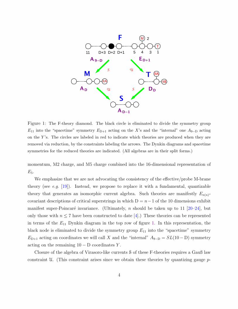
Figure 1: The F-theory diamond. The black circle is eliminated to divide the symmetry group

E11 into the “spacetime” symmetry ED+1 acting on the X’s and the “internal” one A9−D acting

on the Y ’s. The circles are labeled in red to indicate which theories are produced when they are

removed via reduction, by the constraints labeling the arrows. The Dynkin diagrams and spacetime

symmetries for the reduced theories are indicated. (All algebras are in their split forms.)

momentum, M2 charge, and M5 charge combined into the 16-dimensional representation of

E5.

We emphasize that we are not advocating the consistency of the effective/probe M-brane

theory (see e.g. [19]). Instead, we propose to replace it with a fundamental, quantizable

theory that generates an isomorphic current algebra. Such theories are manifestly En(n)-

covariant descriptions of critical superstrings in which D = n−1 of the 10 dimensions exhibit

manifest super-Poincare invariance. (Ultimately, n should be taken up to 11 [20–24], but

only those with n ≤ 7 have been constructed to date [4].) These theories can be represented

in terms of the E11 Dynkin diagram in the top row of figure 1. In this representation, the

black node is eliminated to divide the symmetry group E11 into the “spacetime” symmetry

ED+1 acting on coordinates we will call X and the “internal” A9−D = SL(10−D) symmetry

acting on the remaining 10−D coordinates Y .

Closure of the algebra of Virasoro-like currents S of these F-theories requires a Gauß law

constraint U. (This constraint arises since we obtain these theories by quantizing gauge p-

4

forms.) It also requires “strong sectioning”: solving S = 0 on the tensor algebra of the Hilbert

space. Doing this spontaneously breaks ED+1 → GL(D + 1), the symmetry group of (D + 1)-

dimensional M-theory. (Abelian factors GL(1) do not appear in Dynkin diagrams.) Alter-

natively, solving U = 0 reduces ED+1 → SO(D,D) and the manifestly T-duality-covariant

description of the D-dimensional type-II string [25–27] is recovered. Solving both reduces

ED+1 → GL(D) of S(tring)-theory.

The Virasoro-like constraints S of the En(n) theory generate translations on the worldvol-

ume [2] (see also eq. 2.11 below). Since they also transform in a fundamental representation

of En(n), the target space symmetries are mixed up with the worldvolume ones. To be more

explicit, let us denote the target space Lorentz group by G (= En(n)) and the worldvolume

Lorentz group by L. As much of the analysis is canonical, the basic worldvolume symmetry

is Hamiltonian. We refer to this formalism and its structure group interchangeably as “H”.

Thus, the canonical analysis reduces L→ H and the statement becomes that the G-covariant

constraints S transform in the defining representation of H. This is only possible if G has a

subgroup that is not only isomorphic to H but is, in fact, identified with it.

For low ranks, we have shown that these theories arise from the canonical analysis of

selfdual p-forms on certain branes [2, 3]. Such descriptions have Lagrangian symmetry, and

we again refer to both this formulation of the theory and its underlying group as “L”. Then

the group structures can be summarized as G ⊃ H ⊂ L. In this article, we extend the

constraint algebra by including the Virasoro operators T associated with τ -development (Sa

generates only the translations in σa; cf. eq. 2.11) and use it to study the L(agrangian)

formulation of our theories.

We conclude this introduction with an outline of our presentation. We begin by extending

the worldvolume constraint algebra in the H(amiltonian) formalism in section 2. Currents

and constraints for the bosonic theory are reviewed in 2.1, and their algebra is worked out in

section 2.2. In section 2.3, we review the derivation of the D- and C-brackets (the F-theory

generalizations of the exceptional Lie derivative and bracket on the target).

Closure of the constraint algebra requires the Gauß law and Laplace constraints U and

V. We give an interpretation of these constraints in section 3 as an F-theory generalization

of de Rham forms, or “F-orms” for brevity. In particular, in section 3.1, the H-covariant

form of the field strengths is given in terms of differentials related to the Gauß constraint.

5

This and the Laplace constraint are studied in sections 3.2 and 3.3 where they are related

to the existence of a differential on a complex of F-orms consisting of the gauge parameters,

fundamental fields, field strengths, Bianchi identities, and so on. This complex is constructed

explicitly in section 3.4 in terms of L-covariant field strengths.

In section 4, we complete this bosonic F-theory to the critical superstrings by intro-

ducing the scalars and Green-Schwarz fermions. We define the κ symmetry generators Bα

corresponding to the first-class part of the spinorial constraints Dα. We then investigate

the L(agrangian) description of the theory by performing a Legendre transformation on the

H(amiltonian) action in section 4.2. The result is manifestly supersymmetric in the target

space but has a peculiar structure on the worldvolume: Although it is covariant by con-

struction, the worldvolume metric has only d (= dimension of worldvolume) independent

components instead of the expected 12d(d + 1). Such Lagrangians are studied in section 4.4

by constructing them from selfdual F-orms. They have Wess-Zumino terms of “heterotic”

type (no Θ4 term). Finally, we reduce these actions from F-theory to T-theory (§4.5) by

solving the Gauß law sectioning condition thereby showing how the type-II Wess-Zumino

term is generated.

Our conclusions are reviewed in section 5. We include three appendices A, B, and C

summarizing our notation, the symmetry structure of the theories, and the explicit form of

the Clebsh-Gordan-Wigner tensor defining the fundamental currents for each dimension.

2 Current Algebra

Consider the theory of a chiral p-form X on a d = 2(p+1)-dimensional worldvolume with

split signature. For p = 0, this describes a “right-moving” scalar on a (1 + 1)-dimensional

worldsheet. For p > 0 these models are higher-dimensional-worldvolume generalizations

of the string. The stress-energy tensor on the worldvolume T(+)ab = 1

4p!F

(+)a

c1...cpF(+)bc1...cp

is constructed from the selfdual part of the (p + 1)-form field strength F = dX. The

Hamiltonian analysis of this system proceeds by singling out a time-like coordinate τ and

splitting the worldvolume coordinates (σa) → (τ, σa). The stress-energy tensor splits as

T(+)ab → (Tab, S

a,T).

In previous work on U-duality-covariant strings [2–4], we focused on the constraints Sa

6

which simultaneously generate σ-translations on the worldvolume and dynamically impose

the strong section condition in the target theory. In this section we supplement that anal-

ysis to include the Virasoro constraint T needed for a complete description of the F-brane

dynamics.

2.1 Constraints

The chiral p-form interpretation is only straightforward for strings with D < 5. In general,

the more appropriate language for F-theory is in terms of the fundamental representations

Ri of En (for i = 1, . . . , n and n = D + 1). In the numbering of the nodes of the E11 diagram

indicated in figure 1, Sa is valued in the R1 representation, and the dynamical parts of the

gauge field XA (or its conjugate momentum PA) are valued in the Rn representation. We

summarize the currents/constraints and the En representations in which they are valued in

figure 2.

Y P

U

S

Figure 2: Fundamental representations and currents: P denotes the momentum current of the

theory. S and U are the section and Gauß constraints. The scalars Y will be added in section 4.

The momenta PA conjugate to XA are defined by the equal-τ commutator

[PA(1), XB(2)] = −iδBAδ(1− 2). (2.1)

In the Hamiltonian analysis, the selfdual part F (+) of the field strength defines the En-

covariant current

PA ≡ PA + ηABc∂cXB, (2.2)

while the anti-selfdual part

PA ≡ PA − ηABc∂cXB (2.3)

is the second-class constraint. The η symbols are the Clebsch-Gordan-Wigner coefficients

mapping Rn ⊗Rn → R1. They are used to define the section constraints Sc ≡ 14PAη

ABcPB.

7

To extend to T ≡ S0, we need a symmetric G-invariant pairing η0 on Rn. We will simply

assume such a tensor exists (it does for low ranks) and derive the conditions it must satisfy.

In terms of these G-tensors, the section and Virasoro constraints are Sc ≡ 14PAη

ABcPB and

T ≡ 14PAη

AB0PB. To reduce clutter, we will often suppress Rn indices, with tensors matrix-

multiplied. Furthermore, we combine worldvolume indices c = 0, c runing over both τ and σ

values so that we can write

Sc = 14PηcP . (2.4)

The equal-τ commutator of the selfdual currents is

[PA(1),PB(2)] = 2iηABc∂cδ(1− 2). (2.5)

From this we compute the brackets of the currents with the constraints

[Sa(1),P(2)] = iηcηa∂cδ(1− 2)P(1) (2.6)

On functions f(X)

[PA, f ] = −i∂Af δ, (2.7)

so

[Sa, f ] = − i2(∂fηaP) δ. (2.8)

We can relate this generator to worldvolume diffeomorphisms by introducing its analog con-

structed from the second-class constraints (2.3) and observing that

Sa − Sa = 14(PηaP− PηaP) = 1

4(P + P)ηa(P− P) = ∂bXηbη

aP = ∂aXP − ∂bXUab P, (2.9)

where the last equality is the definition of U (cf. ref. [4]). It defines the Gauß law constraint

of reference [2]:

Ua ≡ Uab ∂

bP with Uab = δab − ηbηa . (2.10)

(This matrix satisfies Uab U

bc ∝ Ua

c , so it defines a projector Rn ⊗ R1 → R2 associating U to

the top node of figure 2: cf. §3.2 and §3.3.) Thus, we have found that

[Sa − Sa, f ] = −iδ ∂af (2.11)

8

up to Gauß law sectioning (i.e. U = 0 on the tensor algebra of the Hilbert space).

As we are working in the Hamiltonian formalism, the quantum brackets are equal-τ

commutators and ∂0 does not appear explicitly. Instead, τ -evolution is determined by the

Heisenberg operator

d

dτ=

∂

∂τ+ iH. (2.12)

Because of this, ∂0 will never be generated on the right-hand-side of any equal-τ bracket.

(We will define the Hamiltonian in terms of the constraints in §4.2, cf. eq. (4.12).)

2.2 Algebra

We are now in a position to compute the equal-τ bracket of Sa with itself. Using the

identity

∂aδ(1− 2)A(1)B(2) = ∂aδ(1− 2)AB + 12δ(1− 2)A

↔∂ aB (2.13)

with currents on the right-hand-side evaluated at the “mid-point” 12[(1) + (2)], we find

[Sa(1), Sb(2)] = i2∂cδ(1− 2)P(1)ηaηcη

bP(2)

= i2∂cδ(1− 2)Pηaηcη

bP + i4δ(1− 2)Pηaηcη

b↔∂ cP. (2.14)

The first term on the right-hand side is symmetric. For this to be a Schwinger term, (i.e.

close onto ∂δS), there must be a tensor k such that

12η(aηcη

b) = kabcd ηd. (2.15)

The second term in (2.14) is anti-symmetric. Expanding the last two η’s,

Pηaηcηb↔∂ cP = Pηa(δbc − U b

c )↔∂ cP = −PηaU b

c

↔∂ cP = ∂c(PηaU b

cP)− PηaU bc∂

cP, (2.16)

with the δ term canceling by symmetry of η. (We extend the previous definition of U ba in the

obvious way to U ba = δba − ηaηb.) The first term can be expanded as

η[aU b]c = η[aδb]c − η[aηcη

b] (2.17)

9

but the η3 term is anti-symmetric. For the second term, we use the definition of the Gauß

law to write

PηaU bc∂

cP = Pη[a(Ub] + Vb]X

), (2.18)

where

Va ≡ 12V abc∂

b∂c with V abc = Ua

(bηc) . (2.19)

Collecting results, we find the equal-τ bracket of the S constraints

[Sa, Sb] = i∂cδkabcdSd − i

2δ∂[aSb] − i

4δPη[aUb] − i

4δPη[aVb]X . (2.20)

This algebra holds modulo sectioning and with the understanding that ∂0 is to be set to zero

(cf. comment under eq. 2.12).

In section 3, we will derive conditions on the Schwinger tensors k. Their explicit form is

dimension-dependent, but a common feature is that they satisfy

η0ηaη0 = ηabη

b or k00ab = ηab. (2.21)

(This is a generalization of the “factorization of the vielbein” eq. 4.3 reference [2].) Here, ηab

is the flat metric on the worldvolume (which we write explicitly to distinguish it from ηABc

and ηABc).

To complete the analysis of the worldvolume constraint algebra, we need to know the

quantum brackets with the Gauß law constraint and worldvolume sectioning. However,

[Ua,P] = iVaδ. (2.22)

Thus, solving Va = 0 guarantees that Ua commutes with the selfdual currents and therefore

with everything. (We will give an alternative derivation of this constraint in §3.) Thus, (2.20)

gives the non-trivial part of the algebra of constraints defining the theory F. Truncating

Sa → Sa, we recover the algebra of references [2–4].

Worldvolume reparameterizations by a vector field (ξa) = (ξ0, ξa) are generated by

δξ = i

∫dd−1σ ξaS

a. (2.23)

10

The worldvolume diffeomorphism algebra closes up to constraints as

[δξ, δξ′ ] = δξ′′ with ξ′′a = −12kcdbaξc

↔∂ bξ′b − 1

2∂b(ξ[bξ

′a]). (2.24)

The worldvolume gauge algebra includes, besides the reparameterizations above, the trans-

formations generated by the Gauß constraint with parameter λAa :

δλ = i

∫dd−1σ λaU

a. (2.25)

In the remainder of this section, we will use these constraints to compute the algebra of

target space diffeomorphisms.

2.3 Brackets

The symmetries generated by the selfdual currents on the worldvolume of a string are

generalizations of the diffeomorphisms of the target space. On general grounds, then, the

target space symmetries generated by the currents must include the diffeomorphism sym-

metries of the En(n) exceptional field theory. To show this explicitly, we first compute the

commutator of two worldvolume currents V AI PA(σi) with I = 1, 2:

[V1P(1), V2P(2)] = 2i∂aδV1ηaV2 − iδV[1∂V2]P + iδV[1ηa∂aV2] (2.26)

This can be simplified using the relation

∂af = ∂aX∂f = (ηbηa + Ua

b )∂bX∂f = 12∂fηa(P− P) + ∂bXUa

b ∂f. (2.27)

Then, modulo second class constraints and Gauß law sectioning,

[V1P(1), V2P(2)] = 2i∂aδV1ηaV2 − iδ[δACδ

BD − 1

2ηABaηCDa

]V C

[1 ∂AVD

2] PB. (2.28)

The “D- and C-brackets” [26,27] follow from this by integrating one or both of these currents

over the worldvolume respectively. Such integrated currents

Λi = i

∫dd−1σ λiP (2.29)

are the F-theory analogs of vector fields in the target space.

11

When both currents are integrated, we obtain the C-bracket

[Λ1, Λ2] = Λ12 with λA12 = −(δACδ

BD − 1

2Y AB

CD

)λC[1↔∂Bλ

D2] (2.30)

where

Y ABCD = ηABaηCDa (2.31)

is the projector from the symmetric product of Rn with itself onto R1. This Y -tensor was

defined in reference [28]. This is the F-theory analog of the generalized Lie bracket: When

it is truncated to massless modes, we recover the Courant bracket of exceptional geometry

[28]. Thus, the higher-dimensional worldvolume F-theory is a generalization of the string

worldsheet in which target space diffeomorphisms are enlarged to the En(n) transformations of

“exceptional field theory” [28–40]. Further truncation of the exceptional coordinates reduces

the exceptional field theory (with “dual” coordinates) to the En(n) version of generalized

geometry (without) [41, 42].

When only one of the two currents is integrated, we obtain the (asymmetric) D-bracket.

From (2.28) we find

[Λ, V P] = δλV P with δλVA = λB

↔∂BV

A + Y ABCD(∂Bλ

C)V D (2.32)

By comparison, we see that the massless truncation of this D-bracket is the generalized Lie

derivative (also known as the “Dorfman bracket” in the exceptional geometry literature), at

least when equation (2.31) is satisfied. This equation holds for D ≤ 5 and holds in D = 6

(corresp. to E7) up to a new constraint called W in reference [4]. (We will mostly ignore W

in this work.)

Backgrounds are introduced as usual:

PA = EAMPM . (2.33)

Under spacetime gauge transformations (cf. eq. 2.32),

δλEAM = λN

↔∂NEA

M + Y MNPQ(∂Nλ

P )EAQ. (2.34)

The background satisfies an “orthogonality constraint” of the form [2]

ηABcEAMEB

N = ηMNpecp (2.35)

which can be interpreted as fixing part of the worldvolume metric in terms of the spacetime

metric. (It cannot be other way around, as the worldvolume fills only part of the spacetime.)

12

3 Worldvolume F-orms

In reference [43], we introduced the notion of F-orms as an F-(super)gravity generalization

of de Rham forms in the target space. (This was done explicitly only for the case of E4(4) =

SL(5).) Such target space F-orms exist because of the S section condition. We now consider

the worldvolume analog of this construction [3].

3.1 H Field Strengths

The constraints U, V, ... can be interpreted as the existence of a differential on the space

of exceptional exterior forms, or worldvolume “F-orms”. We have seen this already in the

structure of the currents: The bosonic (anti)selfdual field strengths (currents) (2.2) and (2.3)

in the H(amiltonian) form

F (±) = P ± ηc∂cX ≡ η0Fτ ± Fσ (3.1)

come with the gauge invariance generated by (2.10):

Ua = Uab ∂

bP with Uab = δab − ηbηa.

When translated to Lagrangian language (see below), Fτ will be the part of the full field

strength carrying a τ (0) index, while Fσ is the part of the field strength defined in the σ

subspace.

We can thus construct a series of differential relations in this subspace (to be extended to

the full worldvolume below) representing gauge transformations, field strengths, and Bianchi

identities. (This generalizes the special case of de Rham forms; see below.) Using the notation

d ≡ ηa∂a , da ≡ UTa

b ∂b = ∂a − ηad , dTa ≡ ∂bUab = ∂a − dηa (3.2)

we have

δX = daλa , Fσ = dX , Ba = dTaFσ (3.3)

defined on the gauge parameters λAa , fields XA, field strengths FσA, and Bianchi identities

BaA. We thus have an analog of Hodge duality

λAa ↔ BaA , XA ↔ FσA (3.4)

13

For these equations to be compatible, the d’s must satisfy the identities

dda = dTad = Va → 0 (3.5)

(the two expressions are equivalent), which requires the V constraint.

3.2 Only U

The simplest examples are those where the V and W constraints are absent. For our

purposes, that means D ≤ 3 for the X’s (or arbitrary scalars Y and their duals Y ; we defer

their discussion to section 4).

Peeling off the two ∂’s from the d2 identity (3.5), we then have

δc(aηb) − η(aηcηb) = V c

ab = 0. (3.6)

(Note that the second term is the (dual of the) Schwinger tensor eq. 2.15.) From this identity

follows

ηcηaηbηc = (I − ηcηc)ηbηa + (ηcηc)δ

ba (3.7)

so

U2 = (I + ηaηa)U (3.8)

If ηaηa ∼ I, we also have

ηaηa = d2I (3.9)

so U/(d2

+ 1) is a projection operator.

These cases are essentially just differential forms, so we now consider the latter directly.

In that case we replace the matrix product with the wedge product. We next translate

the standard representation of the algebra of differential forms as Clifford algebras into our

notation. We define

ηa = dσa , ηa = δa, (3.10)

where δa is the dual to dσa: It acts only on it, as

δadσb = δab − dσbδa. (3.11)

14

(The sign is from the usual antisymmetry of the wedge product.) This is the anticommutation

relation

δa, dσb = δab (3.12)

of fermionic creation and annihilation operators, whose representation space is that of anti-

symmetric tensors of all ranks. (It is also the direct sum of two Clifford algebras, representing

left and right multiplication of those algebras on a representation space of square matrices,

which can be expressed in a basis of products of Dirac γ-matrices. But the identification in-

stead with fermionic oscillators manifests the GL symmetry instead of just the SO of Clifford

algebras.) As a result, the η3 identity (3.6) is easily satisfied, since

dσ(a ∧ dσb) = 0. (3.13)

We then find that

d ≡ ηa∂a = dσa∂

a (3.14)

is the usual exterior derivative, as well as

da = dηa , dTa = ηad (3.15)

For our purposes, the “A ” indices on the η’s would run over only selfdual and anti-selfdual

tensors, or other dual pairs (like Y and Y ), not the full range of all antisymmetric tensors.

3.3 U and V

Generalizing to include the V constraint will not modify the d identities, but does change

the η3 identity used to derive them: Here we consider the cases with the V constraint but

without W [4] (i.e. D = 4 and 5).

For the case D = 4, we have3

V cab = 1

2ηabη

cdηd. (3.16)

3Note that this is compatible with (2.21) and can be combined with it to give

η(aηcηb) − δc(aηb) = −ηabηcdηd.

15

The extra term produces the constraint [3]

Va = ηabηbV with V ≡ 12ηab∂

a∂b (3.17)

when this identity is multiplied by ∂a∂b: Thus

dda = dTad = ηabηbV→ 0 (3.18)

The new term breaks the G symmetry to an orthogonal group. Its coefficient is fixed

by the requirement that the U matrix be proportional to a projection operator, which also

requires the γ-matrix-like identity

ηaηb + (ηbcηc)(ηadηd) = δab . (3.19)

(This implies the previous identity (3.16).) It also implies

ηaηa = d−12I (3.20)

ηcηaηbηc = −d−5

2ηbηa + d−3

2δba (3.21)

so U/d−12

is a projection operator.

In D = 5 we have for the group E6, instead of the orthogonal metric ηab, the totally

symmetric symbol dabc for the 27 representation and dabc for the 27′. They satisfy the

“Springer relation” [44–46]

18defgde(abdcd)f = 1

6δg(adbcd) (3.22)

or, eliminating redundant terms,

defg(deabdcdf + deacddbf + deaddbcf ) = δgadbcd + δgbdcda + δgcddab + δgddabc. (3.23)

In this case, since the a and A indices are the same, we identify ηabc = dabc, so this is our η3

identity:

V cab = 1

2ηabeη

cdeηd − 12Ic ⊗ ηab, (3.24)

where we have abbreviated

(Ic ⊗ ηab)de ≡ δc(dηe)ab. (3.25)

16

Now the V constraint is the worldvolume dual of the S constraint, namely

Va = 12ηabc∂

b∂c ↔ Sa = 14ηabcPbPc, (3.26)

dda = dTad = ηabcηbVc − Ia ⊗ V→ 0, (3.27)

where we have used the shorthand notation

(Ia ⊗ V)bc ≡ δa(bVc). (3.28)

3.4 L Field Strengths

We now generalize the above results to the full worldvolume (τ and σ), but still written

in H-covariant notation. The gauge parameters are λAa ; the bosons are now XA, XAa (U

multipliers); their field strengths are FAτ , FσA. Then we have

δX = ∂a(λa − ηbηaλb) , δXa = ∂0λa (3.29a)

Fσ = ∂a(ηaX) , Fτ = ∂0X − ∂a(Xa − ηbηaXb) (3.29b)

(∂bηbηa − ∂a)Fσ = 0 , ∂0Fσ − ∂a(ηaFτ ) = 0 (3.29c)

(Compare 4D electromagnetism in 3-vector notation. Supersymmetrization will be considered

below.)

With the help of the d notation, these equations simplify to

δ

(X

Xa

)=

(da

∂0

)λa (3.30a)

(Fσ

Fτ

)=

(d 0

∂0 −da

)(X

Xa

)(3.30b)

(B

Ba

)=

(−∂0 d

dTa 0

)(Fσ

Fτ

)(3.30c)

BBa =(dTa ∂0

)( B

Ba

)(3.30d)

17

where the B’s are the Bianchi identities, and BB is the Bianchi identity of the Bianchi

identities. This implies a generalization of the Hodge duality (3.4) considered in the σ space,

as expected from adding 1 dimension:

λAa ↔ BBaA ,

(XA

XAa

)↔

(BA

BaA

),

(Fσ A

FAτ

)↔

(FAτ

−Fσ A

). (3.31)

In the special case of true differential forms given above, this is easily seen to reduce to

the usual (in σ ⊕ τ notation): Then we have the replacments

λa → λ = ηaλa , Xa → X0 = ηaXa , Ba = ηaB0 , BBa = ηaBB. (3.32)

The σ forms can then be upgraded to στ forms by

d = d+ dτ ∂0 (3.33)

and

X = X + dτ ∧X0 , F = Fσ + dτ ∧ Fτ , B = B0 − dτ ∧B. (3.34)

Then the equations (3.30) collapse to

δX = dλ , F = dX , B = dF , dB = dτ ∧BB + dB0. (3.35)

4 Critical Superstrings

Critical U-duality-covariant superstrings were constructed for ranks n ≤ 7 in [4]. They

are obtained from the non-critical D-dimensional U-duality-covariant bosonic superstrings

by completing with D′ = 10 − D spacetime coordinate fields Y a′ (and their duals Yaa′) and

32 fermionic Green-Schwarz fields Θα. We provide a summary of indices and symbols in

appendix A.

4.1 Supersymmetry

Finally, we introduce the 32 Green-Schwarz fermionic worldvolume scalars Θα. These can

be contracted with (spacetime) Pauli-like matrices (γA)αβ. Introducing the dual matrices

(γA)αβ, they close onto worldvolume Dirac-like matrices (Γa)αβ as [4]

γAγB + γBγA = 2ηABcΓc, (4.1)

18

where we take the τ component (Γ0)αβ = δ

βα to be the unit matrix.

The supersymmetry currents are

D = Π + γΘ (P− ηcχc) (4.2a)

P = P + ηa(∂aX + 2χa) (4.2b)

Ωaα = −2i∂aΘα (4.2c)

P = P − ηa∂aX (4.2d)

where

χAa ≡ −iΘγA∂aΘ. (4.3)

The “selfdual” supercurrents DPΩ satisfy the deceivingly “familiar” bracket relations [4]

D,D = 2 γ P δ and [D,P] = 2 ηc γ Ωc δ, (4.4)

while the anti-selfdual (non-super) current P commutes with the rest.

The Hamiltonian action is invariant under the supersymmetry transformation generated

by

q =

∫ [Π − γΘ

(P− 5

3ηaχ

a)]

(4.5)

inducing

δΘ = ε , δXA = iεγAΘ , and δPA = −iηABc εγB∂cΘ. (4.6)

As usual, the constraints D = 0 are mixed first and second class. The first class part

defines the κ symmetry generator

B = P/D = PAγAD. (4.7)

Its components close onto the S generators

Bα,Bβ = 2(P/Γa)(αβ) Sa δ + . . . (4.8)

modulo terms containing the second class constraint D. (The B part of the algebra is formally

the same as the analogous string algebra in reference [47] under the replacement A→ S.) The

worldvolume gauge algebra includes, besides the reparameterizations (2.23) and the trans-

formations (2.25) generated by the Gauß law constraint, the κ symmetry transformations

δκ = i

∫dd−1σ καB

α. (4.9)

19

4.2 H Action

With the constraints Sa closing on Gauß’s law Ua and worldvolume sectioning Va, we are

in a position to write down the action of the worldvolume theory in Hamiltonian form. To

this end, we first impose worldvolume sectioning [3]

Va = 0 (4.10)

and define the action on the space of solutions to this constraint. Then, in Hamiltonian form

it is given by SH =∫LH with

LH = −.XP + i

.ΘΠ +H (4.11)

in terms of the Hamiltonian

H = λD −XaUa + 1

2`0(T + T) + 1

2`a(S

a − Sa). (4.12)

Here Xa, `0, and `a are the Lagrange multipliers for the constraints U (2.10) and S, T (2.4),

respectively. (This name for the U multiplier will be justified in §4.3.) We recall here that

the tilded versions of the constraints are defined by replacing the selfdual currents P with

the anti-selfdual currents P. This Lagrangian is manifestly spacetime supersymmetric and

H-invariant. G-invariance requires coupling to a background as introduced in section 2.3.

4.3 L Action

We now set D → 0 as a second-class constraint to solve for the momentum Π conjugate

to Θ, and integrate out P using its equation of motion. Since P and P are to be identified

with the selfdual and anti-selfdual field strengths, we write their resulting forms as

P = η0Fτ + Fσ and P = η0Fτ − Fσ. (4.13)

We then find that

Fτ = ∂0X + χ0 − ∂a(Xa − ηbηaXb) and Fσ = ηa(∂aX + χa) (4.14)

(as well as P = η0Fτ − ηaχa) are simply the result of supersymmetrizing the Lagrangian

bosonic field strengths obtained previously by the substitution ∂X → ∂X + χ, as expected

20

from the usual invariant worldvolume currents dX − iΘγdΘ and dΘ as the left-invariant

1-forms on the target space.

The Lagrangian is then

L = `012Fση

0Fσ − `−10

12(Fτ − `mηmFσ)η0(Fτ − `nηnFσ) + LWZ (4.15a)

LWZ = −F σχ

0 +F τηaχ

a = −F σFτ +

F τFσ, (4.15b)

where in the Wess-Zumino term LWZ ,F stands for the χ = 0 part of F .

This action can be rewritten in the form

L =√−g 1

2(Fση0Fσ − Fτη0Fτ ) + LWZ (4.16)

where

√−g = `0 , Fσ = Fσ , Fτ = `−1

0 (Fτ − `mηmFσ), (4.17)

from which we find that the worldvolume vielbein eam takes the simple form

eam = δam , e0m = `−1

0 (1,−`m) (4.18)

(the former from Fσ, the latter from Fτ ).

For example, in the case of standard differential forms considered previously (cf. section

3.2), flattening the indices on Fσ (none of which are “0”) is trivial, while on Fτ (only one “0”

index), the ηm (δm) picks off one “m” index from Fσ.

Note that there are no Θ4 terms in the Wess-Zumino term, since this is a “heterotic” type

of construction. They will reappear upon reduction of F-theory to T-theory below: As usual

in dimensional reduction, selfdual theories reduce to non-selfdual theories.

4.4 Actions from Selfduality

To gain some insight into the structure of the Lagrangian (4.16), we derive it covariantly.

A useful method to treat actions for selfdual theories is to use covariant, non-selfdual actions,

and then impose selfduality separately. A well-known way to derive the corresponding field

equations compatible with selfduality is by replacing field strengths with their duals in the

Bianchi identities. We thus begin with the general gauge transformations, field strengths,

21

and Bianchi identities for the bosons in F-theory, supersymmetrized, in H-covariant form.

For simplicity, we work in the “conformal” gauge eam = δam for the worldvolume metric.

After reintroducing Θ, the gauge transformations are unchanged (δΘ = 0), and the field

strengths are supersymmetrized by replacing ∂X → ∂X + χ (cf. eq. 4.14). For ease of

reference, we reproduce them here in the new notation:

Fσ = dX + ηaχa , Fτ = ∂0X − daXa + χ0. (4.19)

The Bianchi identities then become the analog of dF = dχ:

(∂bηbηa − ∂a)Fσ = 1

2(ηbηaηc − δbaηc)∂[bχc] and ∂0Fσ − ∂a(ηaFτ ) = ηa∂

[0χa], (4.20)

where

∂[aχb] = −i(∂[aΘ)γ(∂b]Θ) (4.21)

showing supersymmetry invariance.

For consistency with the selfduality condition P = 0, that is

Fσ = η0Fτ (4.22)

(cf. eq. 4.13), variation of the metric part of the non-selfdual action must give exactly the

result of switching Fσ ↔ η0Fτ in the Bianchi identities, less the χ correction terms from the

Wess-Zumino part of the action: After integration by parts,

δ 12(Fση

0Fσ − Fτη0Fτ )→ δX[∂0η0Fτ − ∂a(ηaη0Fσ)] + δXa(∂bηbη

a − ∂a)η0Fτ . (4.23)

This implies the necessity of the Wess-Zumino terms

LWZ = −Xηa∂[0χa] −Xa12(ηbη

aηc − δab ηc)∂[bχc]

→F τFσ −

F σFτ (4.24)

after integration by parts, showing gauge invariance. (Modifying the WZ terms by integration

by parts will change the expressions for the currents (4.2) and (4.5) by a canonical trans-

formation [4].) The result for L then agrees with that obtained by Legendre transformation

(4.16) in the gauge `0 = 1, `m = 0 (the flat case).

22

4.5 Reduction F → T

The Lagrangian (4.16) has a heterotic-type Wess-Zumino term due to the doubled nature

of the Green-Schwarz fermions. In this section, we explain how the type-II action of the

underlying string is generated.

Dimensional reduction from F-theory to T-theory comes from solving the Gauß constraint

U. (Also the V,W constraints are solved, but we’ll ignore those here for simplicity.) Since

both ∂ and P are bispinors, we can write this constraint in matrix notation as

U = ∂P − P∂ = 0. (4.25)

(See appendix B.)

The doubled spinor index is thereby divided into left and right halves: Choosing a solution

where ∂ picks one particular direction, its single γ-matrix can be chosen block diagonal,

forcing P to also be so. Thus we have a single σ for the worldsheet, while P has lost its

Ramond-Ramond (LR) pieces, as seen from the commutation relations D,D ∼ P .

While the effect on the metric terms in the action is to simply drop the LR terms, the

WZ term generates a Θ4 term: Since P ∼ ∂X + χ, the ∂X (F ) factor there is replaced by

−χ for the LR piece. This results in χLR ∧ χLR ∼ χLL ∧ χRR, as in the usual Green-Schwarz

action.

5 Conclusions

In this work, we have given the Lagrangian formulation for the F-theory of critical super-

strings in which the En(n) U-duality symmetry is manifest for rank n ≤ 7. (This corresponds

to critical superstrings in a D + (10 − D)-dimensional split with D = n − 1.) To do this,

we first extended the Hamiltonian description of the current algebra of constraints gener-

ating worldvolume translations [4] to include the generator responsible for the dynamics of

the fundamental brane. We then constructed the Hamiltonian action from the constraints

and performed a Legendre transformation to the Lagrangian form. This gives the world-

volume metric in terms of the Lagrange multipliers of the Hamiltonian formulation (4.18).

The resulting theory has the peculiar property that only d components of the d-dimensional

worldvolume metric are needed for a covariant description instead of the usual 12d(d + 1).

23

(Thus, covariance is not manifest on the worldvolume except perhaps in a manner analogous

to [48].) Consequently, they can all be gauged away in an analog of conformal gauge for the

string (in contrast to the usual attempts to quantize the membrane in which the worldvolume

gravity is dynamical).

In this new formulation, the worldvolume fields can be interpreted as an F-theory general-

ization of the ordinary p-form gauge fields of Maxwell-like theories. The Gauß law constraint

U is used to define the analog of the exterior derivative operator and the Laplace constraint

V implies that it is a differential. This gives rise to the exceptional geometry analog of the

usual de Rham forms on the worldvolume.

The Lagrangian of the supersymmetric theory resembles that of a heterotic superstring

in that the Wess-Zumino term has no Θ4 terms. This is the structure determined by the con-

sistency between supersymmetry and the selfduality of the field strength of the fundamental

gauge field. Reducing from F to the string by solving the Gauß law sectioning condition, the

familiar Wess-Zumino term of the type-II Green-Schwarz action is recovered.

All formulations of all these theories have a symmetry H dependent only on the dimension

D. (There is also the symmetry H ′ = SO(10− D) which we leave implicit here.) If we limit

our discussion to just the bosonic sector of a theory, then this symmetry is extended to the

group G in the Hamiltonian formalism, and to L in the Lagrangian formalism. Thus ηABa is

an invariant tensor of G, while ηABa is an invariant tensor of L. However, after extending to

supersymmetry by including the fermions, only the H subgroup survives in either formalism:

While the bosons form representations of the larger groups, the fermions are representations

of only H. As familiar from extended supergravity, the larger symmetry can be restored by

including fields of the corresponding coset: In our case, the spacetime (second-quantized)

vielbein E lives on the coset G/H, while the worldvolume (first-quantized) vielbein e lives

on the coset L/H. Thus the background fields E restore G symmetry to the Hamiltonian

formalism (and the resulting spacetime theory), while the Lagrange multipliers e restore L

symmetry to the Lagrangian formalism. In particular, if we ignore allGL(1)’s in the definition

of L, we find L/H has d− 1 generators for D ≤ 5. The consistency of the simultaneous G/H

and L/H cosets is then enforced by the orthogonality constraint (2.35).

24

Acknowledgements

It is a pleasure to thank Machiko Hatsuda for discussions relating our F-theory work to

the brane current algebra approach of references [16,17,49], and Andy Royston and Stephen

Randall for discussions and suggestions that helped to improve the presentation. Wdl3 is

grateful to the Simons Center for Geometry and Physics for hospitality during the viii and ix

Simons Summer Workshops where parts of this project were completed. Wdl3 is supported

by National Science Foundation grants PHY-1214333 and PHY-1521099. Ws was supported

by NSF grant PHY-1316617.

A Notation

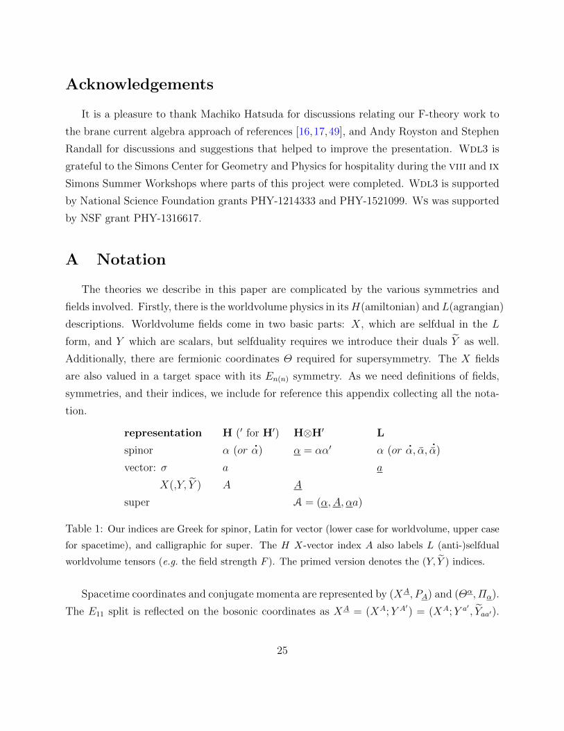
The theories we describe in this paper are complicated by the various symmetries and

fields involved. Firstly, there is the worldvolume physics in itsH(amiltonian) and L(agrangian)

descriptions. Worldvolume fields come in two basic parts: X, which are selfdual in the L

form, and Y which are scalars, but selfduality requires we introduce their duals Y as well.

Additionally, there are fermionic coordinates Θ required for supersymmetry. The X fields

are also valued in a target space with its En(n) symmetry. As we need definitions of fields,

symmetries, and their indices, we include for reference this appendix collecting all the nota-

tion.

representation H (′ for H′) H⊗H′ L

spinor α (or.α) α = αα′ α (or

.α, α,

.α)

vector: σ a a

X(,Y, Y ) A A

super A = (α,A, αa)

Table 1: Our indices are Greek for spinor, Latin for vector (lower case for worldvolume, upper case

for spacetime), and calligraphic for super. The H X-vector index A also labels L (anti-)selfdual

worldvolume tensors (e.g. the field strength F ). The primed version denotes the (Y, Y ) indices.

Spacetime coordinates and conjugate momenta are represented by (XA, PA) and (Θα, Πα).

The E11 split is reflected on the bosonic coordinates as XA = (XA;Y A′) = (XA;Y a′ , Yaa′).

25

We do not need the split of the fermionic coordinates in the main body of this paper, but

as it is important to the symmetry structure of the theory, we refer to it in a condensed

form in appendix B. (It is worked out in detail in ref. [4].) Also in this paper, we do not

differentiate between the momenta for Y and Y but when it is useful, we call the former

Υ and the latter . The entire collection of covariant currents is lumped into the “nacho”

.A = (Dα,PA, Ωαa). (Again, we have little recourse to this symbol in this paper but we

include it for completeness.) The definition of these currents is given in (4.2).

In the H form, because of the E11 split, there is the En(n) part H and the rest H′. We

collect the relevant notation for the indices of this separation in table 1.

B Symmetry

In this section, we give a condensed summary of the target and worldvolume symmetry

structures of the ED+1 theories. The target space symmetry group is called G (= ED+1

throughout this work). It is the symmetry group of the F-theory currents and their bracket

algebra. The Hamiltonian representation of the currents preserves all of G for the bosonic

part but only a subgroupH if the Green-Schwarz fermions are included. This subgroup can be

interpreted as the “rotation” subgroup of a worldvolume Lorentz group L. In this appendix,

we review the relationships between the groups G ⊃ H ⊂ L for various D. Additional details

can be found in reference [4].

Because of the supersymmetric current algebra D,D, both the worldvolume and the

(bosonic) spacetime coordinates σ and X can be written as bispinors, where for (at least)

D ≤ 7 only reality and symmetry constraints need be applied. These are also sufficient

to define the H group. The diagram in figure 3 indicates their index structure and the

corresponding H groups for the physical spacetime dimension D mod 8. The ovals indicate

the range of spinor indices, enclosing the dimensions (D) with equal ranges, before considering

reality properties; outside it increases by a factor of 2 when increasing D by 2. The range is

double that of the corresponding Lorentz group, so starts with 2 for D = 1, 2.

The extension of H symmetry to the L symmetry of the Lagrangian drops the SO and

Sp conditions, and gives two copies of SL (except for D = 10). Thus, in general the number

of generators roughly doubles. The σ’s above include τ , which appears as the trace piece

26

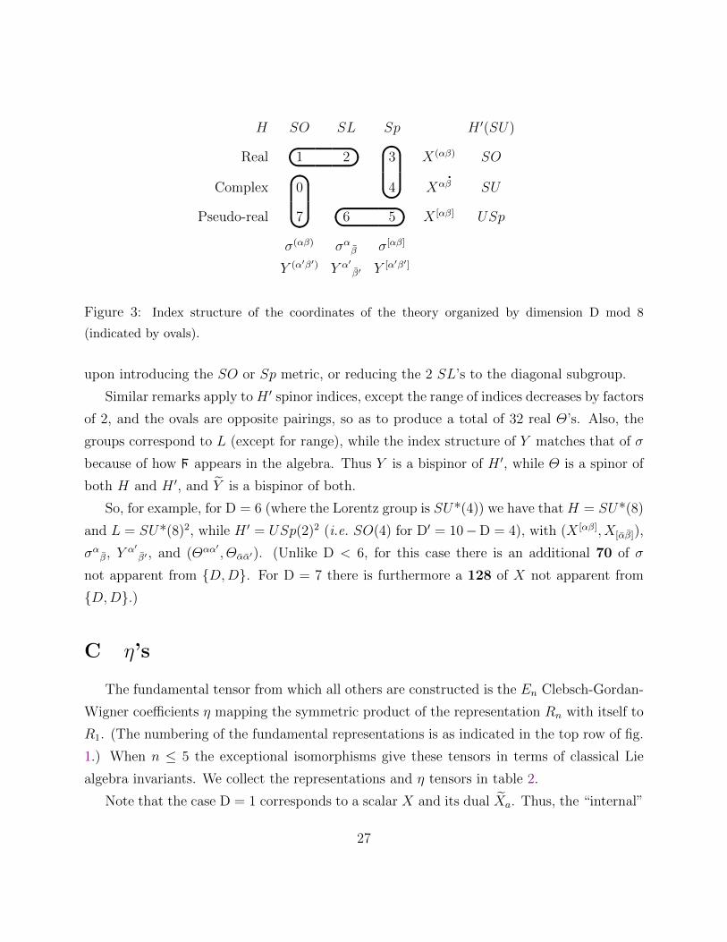
H SO SL Sp H ′(SU)

Real 1 2 3 X(αβ) SO

Complex 0 4 Xα.β SU

Pseudo-real 7 6 5 X [αβ] USp

σ(αβ) σαβ σ[αβ]

Y (α′β′) Y α′β′ Y [α′β′]

b

ad

c

b

ad

c

b

ad

cb

ad

c

Figure 3: Index structure of the coordinates of the theory organized by dimension D mod 8

(indicated by ovals).

upon introducing the SO or Sp metric, or reducing the 2 SL’s to the diagonal subgroup.

Similar remarks apply to H ′ spinor indices, except the range of indices decreases by factors

of 2, and the ovals are opposite pairings, so as to produce a total of 32 real Θ’s. Also, the

groups correspond to L (except for range), while the index structure of Y matches that of σ

because of how appears in the algebra. Thus Y is a bispinor of H ′, while Θ is a spinor of

both H and H ′, and Y is a bispinor of both.

So, for example, for D = 6 (where the Lorentz group is SU*(4)) we have that H = SU*(8)

and L = SU*(8)2, while H ′ = USp(2)2 (i.e. SO(4) for D′ = 10−D = 4), with (X [αβ], X[αβ]),

σαβ, Y α′β′ , and (Θαα′

, Θαα′). (Unlike D < 6, for this case there is an additional 70 of σ

not apparent from D,D. For D = 7 there is furthermore a 128 of X not apparent from

D,D.)

C η’s

The fundamental tensor from which all others are constructed is the En Clebsch-Gordan-

Wigner coefficients η mapping the symmetric product of the representation Rn with itself to

R1. (The numbering of the fundamental representations is as indicated in the top row of fig.

1.) When n ≤ 5 the exceptional isomorphisms give these tensors in terms of classical Lie

algebra invariants. We collect the representations and η tensors in table 2.

Note that the case D = 1 corresponds to a scalar X and its dual Xa. Thus, the “internal”

27

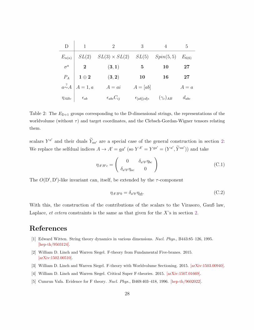
D 1 2 3 4 5

En(n) SL(2) SL(3)× SL(2) SL(5) Spin(5, 5) E6(6)

σa 2 (3,1) 5 10 27

PA 1⊕ 2 (3,2) 10 16 27

a?∼A A = 1, a A = ai A = [ab] A = a

ηABc εab εabcCij ε[ab][cd]e (γc)AB dabc

Table 2: The ED+1 groups corresponding to the D-dimensional strings, the representations of the

worldvolume (without τ) and target coordinates, and the Clebsch-Gordan-Wigner tensors relating

them.

scalars Y a′ and their duals Yaa′ are a special case of the general construction in section 2:

We replace the selfdual indices A→ A′ = aa′ (so Y A′= Y aa′ = (Y a′ , Y aa′)) and take

ηA′B′c =

(0 δa′b′ηbc

δa′b′ηac 0

)(C.1)

The O(D′,D′)-like invariant can, itself, be extended by the τ -component

ηA′B′0 = δa′b′ηab. (C.2)

With this, the construction of the contributions of the scalars to the Virasoro, Gauß law,

Laplace, et cetera constraints is the same as that given for the X’s in section 2.

References

[1] Edward Witten. String theory dynamics in various dimensions. Nucl. Phys., B443:85–126, 1995.

[hep-th/9503124].

[2] William D. Linch and Warren Siegel. F-theory from Fundamental Five-branes. 2015.

[arXiv:1502.00510].

[3] William D. Linch and Warren Siegel. F-theory with Worldvolume Sectioning. 2015. [arXiv:1503.00940].

[4] William D. Linch and Warren Siegel. Critical Super F-theories. 2015. [arXiv:1507.01669].

[5] Cumrun Vafa. Evidence for F theory. Nucl. Phys., B469:403–418, 1996. [hep-th/9602022].

28

[6] E. Bergshoeff, E. Sezgin, and P.K. Townsend. Supermembranes and Eleven-Dimensional Supergravity.

Phys.Lett., B189:75–78, 1987. [inSPIRE entry].

[7] E. Bergshoeff, E. Sezgin, and P. K. Townsend. Properties of the Eleven-Dimensional Super Membrane

Theory. Annals Phys., 185:330, 1988. [inSPIRE entry].

[8] John H. Schwarz and Ashoke Sen. Duality symmetric actions. Nucl. Phys., B411:35–63, 1994.

[hep-th/9304154].

[9] Paul S. Howe and E. Sezgin. Superbranes. Phys. Lett., B390:133–142, 1997. [hep-th/9607227].

[10] Paul S. Howe and E. Sezgin. D = 11, p = 5. Phys. Lett., B394:62–66, 1997. [hep-th/9611008].

[11] Malcolm Perry and John H. Schwarz. Interacting chiral gauge fields in six-dimensions and Born-Infeld

theory. Nucl.Phys., B489:47–64, 1997. hep-th/9611065.

[12] Paul S. Howe, E. Sezgin, and Peter C. West. Covariant field equations of the M theory five-brane.

Phys. Lett., B399:49–59, 1997. [arXiv:hep-th/9702008].

[13] E. Sezgin and P. Sundell. Aspects of the M5-brane. In Nonperturbative aspects of strings, branes and

supersymmetry., pages 369–389. Proceedings, Spring School on nonperturbative aspects of string

theory and supersymmetric gauge theories and Conference on super-five-branes and physics in 5 + 1

dimensions, Trieste, Italy, March 23-April 3 1998. [arXiv:hep-th/9902171].

[14] Paolo Pasti, Dmitri P. Sorokin, and Mario Tonin. Covariant action for a D = 11 five-brane with the

chiral field. Phys.Lett., B398:41–46, 1997. [arXiv:hep-th/9701037].

[15] Igor A. Bandos, Kurt Lechner, Alexei Nurmagambetov, Paolo Pasti, Dmitri P. Sorokin, and Mario

Tonin. Covariant action for the superfive-brane of M theory. Phys. Rev. Lett., 78:4332–4334, 1997.

[arXiv:hep-th/9701149].

[16] Machiko Hatsuda and Kiyoshi Kamimura. SL(5) duality from canonical M2-brane. JHEP, 1211:001,

2012. [arXiv:1208.1232].

[17] Machiko Hatsuda and Kiyoshi Kamimura. M5 algebra and SO(5,5) duality. JHEP, 1306:095, 2013.

[arXiv:1305.2258v3].

[18] Machiko Hatsuda. Private communication.

[19] M. J. Duff, J. X. Lu, R. Percacci, C. N. Pope, H. Samtleben, and E. Sezgin. Membrane Duality

Revisited. Nucl. Phys., B901:1–21, 2015. [arXiv:1509.02915].

[20] M. J. Duff. E8 × SO(16) Symmetry of D = 11 Supergravity. 1985. [inSPIRE entry].

[21] M. J. Duff. Hidden String Symmetries? Phys. Lett., B173:289, 1986. [inSPIRE entry].

[22] Peter C. West. E11 and M theory. Class.Quant.Grav., 18:4443–4460, 2001. [hep-th/0104081].

[23] Alexander G. Tumanov and Peter West. E11 must be a symmetry of strings and branes. 2015.

[arXiv:1512.01644].

[24] Alexander G. Tumanov and Peter West. E11 in 11D. Phys. Lett., B758:278–285, 2016.

[arXiv:1601.03974].

[25] W. Siegel. Two vierbein formalism for string inspired axionic gravity. Phys.Rev., D47:5453–5459, 1993.

[hep-th/9302036].

29

[26] W. Siegel. Superspace duality in low-energy superstrings. Phys.Rev., D48:2826–2837, 1993.

[hep-th/9305073].

[27] W. Siegel. Manifest duality in low-energy superstrings. Proc. of the Conference Strings ’93, Berkeley,

CA (World Scientific), pages 353–363, May 24-29 1993. [hep-th/9308133].

[28] David S. Berman, Martin Cederwall, Axel Kleinschmidt, and Daniel C. Thompson. The gauge

structure of generalised diffeomorphisms. JHEP, 1301:064, 2013. [arXiv:1208.5884].

[29] David S. Berman, Hadi Godazgar, and Malcolm J. Perry. SO(5,5) duality in M-theory and generalized

geometry. Phys.Lett., B700:65–67, 2011. [arXiv:1103.5733v2].

[30] Andre Coimbra, Charles Strickland-Constable, and Daniel Waldram. Ed(d) ×R+ generalised geometry,

connections and M theory. JHEP, 1402:054, 2014. [arXiv:1112.3989v2].

[31] Jeong-Hyuck Park and Yoonji Suh. U-geometry: SL(5). JHEP, 1304:147, 2013. [arXiv:1302.1652v3].

[32] Olaf Hohm and Henning Samtleben. U-duality covariant gravity. JHEP, 1309:080, 2013.

arXiv:1307.0509.

[33] Olaf Hohm and Henning Samtleben. Exceptional Form of D=11 Supergravity. Phys.Rev.Lett.,

111:231601, 2013. [arXiv:1308.1673].

[34] Olaf Hohm and Henning Samtleben. Exceptional Field Theory I: E6(6) covariant Form of M-Theory

and Type IIB. Phys.Rev., D89:066016, 2014. [arXiv:1312.0614].

[35] Olaf Hohm and Henning Samtleben. Exceptional Field Theory II: E7(7). Phys.Rev., D89:066017, 2014.

[arXiv:1312.4542].

[36] Hadi Godazgar, Mahdi Godazgar, Olaf Hohm, Hermann Nicolai, and Henning Samtleben.

Supersymmetric E7(7) Exceptional Field Theory. JHEP, 1409:044, 2014. [arXiv:1406.3235].

[37] Olaf Hohm and Henning Samtleben. Exceptional Field Theory III: E8(8). Phys.Rev., D90:066002,

2014. [arXiv:1406.3348].

[38] Chris D. A. Blair and Emanuel Malek. Geometry and fluxes of SL(5) exceptional field theory. 2014.

[arXiv:1412.0635v1].

[39] Edvard Musaev and Henning Samtleben. Fermions and Supersymmetry in E6(6) Exceptional Field

Theory. JHEP, 03:027, 2015. [arXiv:1412.7286].

[40] Aidar Abzalov, Ilya Bakhmatov, and Edvard T. Musaev. Exceptional field theory: SO(5, 5). JHEP,

1506:088, 2015. [arXiv:1504.01523].

[41] C.M. Hull. Generalised Geometry for M-Theory. JHEP, 0707:079, 2007. [hep-th/0701203v1].

[42] David S. Berman and Malcolm J. Perry. Generalized Geometry and M theory. JHEP, 1106:074, 2011.

[arXiv:1008.1763v4].

[43] William D. Linch and Warren Siegel. F-theory Superspace. 2015. [arXiv:1501.02761].

[44] P. Cvitanovic. Group Theory: Birdtracks, Lie’s, and Exceptional Groups. Princeton University Press,

2008.

[45] T. A. Springer. Proc. Ned. Ak. Wet., A62:254, 1959.

30

[46] T. A. Springer. Proc. Ned. Ak. Wet., A65:259, 1962.

[47] Warren Siegel. Classical Superstring Mechanics. Nucl.Phys., B263:93, 1986. [inSPIRE entry].

[48] Ashoke Sen. Covariant Action for Type IIB Supergravity. 2015. [arXiv:1511.08220].

[49] Machiko Hatsuda and Tetsuji Kimura. Canonical approach to Courant brackets for D-branes. JHEP,

1206:034, 2012. [arXiv:1203.5499].

31