Embed Size (px)
Citation preview
EXTRINSIC LOCAL REGRESSION ON MANIFOLD-VALUED DATA
LIZHEN LIN, BRIAN ST. THOMAS, HONGTU ZHU, AND DAVID B. DUNSON
Abstract. We propose an extrinsic regression framework for modeling data with manifold valued
responses and Euclidean predictors. Regression with manifold responses has wide applicationsin shape analysis, neuroscience, medical imaging and many other areas. Our approach embeds
the manifold where the responses lie onto a higher dimensional Euclidean space, obtains a local
regression estimate in that space, and then projects this estimate back onto the image of the man-ifold. Outside the regression setting both intrinsic and extrinsic approaches have been proposed
for modeling i.i.d manifold-valued data. However, to our knowledge our work is the first to take
an extrinsic approach to the regression problem. The proposed extrinsic regression frameworkis general, computationally efficient and theoretically appealing. Asymptotic distributions and
convergence rates of the extrinsic regression estimates are derived and a large class of examples
are considered indicating the wide applicability of our approach.Keywords: Convergence rate; Differentiable manifold; Geometry; Local regression; Object
data; Shape statistics.
1. Introduction
Although the main focus in statistics has been on data belonging to Euclidean spaces, it is commonfor data to have support on non-Euclidean geometric spaces. Perhaps the simplest example is todirectional data, which lie on circles or spheres. Directional statistics dates back to R.A. Fisher’sseminal paper (Fisher, 1953) on analyzing the directions of the earth’s magnetic poles, with keylater developments by Watson (1983), Mardia and Jupp (2000), Fisher et al. (1987) among others.Technological advances in science and engineering have led to the routine collection of more complexgeometric data. For example, diffusion tensor imaging (DTI) obtains local information on thedirections of neural activity through 3× 3 positive definite matrices at each voxel (Alexander et al.,2007). In machine vision, a digital image can be represented by a set of k-landmarks, the collectionof which form landmark based shape spaces (Kendall, 1984). In engineering and machine learning,images are often preprocessed or reduced to a collection of subspaces, with each data point (animage) in the sample data represented by a subspace. One may also encounter data that are storedas orthonormal frames (Downs et al., 1971), surfaces, curves, and networks.
Statistical analysis of data sets whose basic elements are geometric objects requires a precise math-ematical characterization of the underlying space and inference is dependent on the geometry ofthe space. In many cases (e.g., space of positive definite matrices, spheres, shape spaces, etc), theunderlying space corresponds to a manifold. Manifolds are general topological spaces equippedwith a differentiable/smooth structure which induces a geometry that does not in general adhere tothe usual Euclidean geometry. Therefore, new statistical theory and models have to be developedfor statistical inference of manifold-valued data. There have been some developments on inferencesbased on i.i.d (independent and identically distributed) observations on a known manifold. Suchapproaches are mainly based on obtaining statistical estimators for appropriate notions of locationand spread on the manifold. For example, one could base inference on the center of a distributionon the Frechet mean, with the asymptotic distribution of sample estimates obtained (Bhattacharyaand Patrangenaru, 2003, 2005; Bhattacharya and Lin, 2013). There has also been some considera-tion of nonparametric density estimation on manifolds (Bhattacharya and Dunson, 2010; Lin et al.,2013; Pelletier, 2005). Bhattacharya and Bhattacharya (2012) provides a recent overview of suchdevelopments.
1
arX
iv:1
508.
0220
1v1
[m
ath.
ST]
10
Aug
201
5
There has also been a growing interest in modeling the relationship between a manifold-valuedresponse Y and Euclidean predictors X. For example, many studies are devoted to investigatinghow brain shape changes with age, demographic factors, IQ and other variables. It is essentialto take into account the underlying geometry of the manifold for proper inference. Approachesthat ignore the geometry of the data can potentially lead to highly misleading predictions andinferences. Some geometric approaches have been developed in the literature. For example, Fletcher(2011) develops a geodesic regression model on Riemannian manifolds, which can be viewed as acounterpart of linear regression on manifolds, and subsequent work of Hinkle et al. (2012) generalizespolynomial regression model to the manifold. These parametric and semi-parametric models areelegant, but may lack sufficient flexibility in certain applications. Shi et al. (2009) proposes a semi-parametric intrinsic regression model on manifolds, and Davis et al. (2007) generalizes an intrinsickernel regression method on the Riemannian manifold, considering applications in modeling changesin brain shape over time. Yuan et al. (2012) develops an intrinsic local polynomial model on thespace of symmetric positive definite matrices, which has applications in diffusion tensor imaging. Adrawback of intrinsic models is the heavy computational burden incurred by minimizing a complexobjective function along geodesics, typically requiring evaluation of an expensive gradient in aniterated algorithm. The objective functions often have multiple modes, leading to large sensitivityto start points. Further, existence and uniqueness of the population regression function holds onlyunder relatively restrictive conditions. Therefore, usual descent algorithms used in estimation arenot guaranteed to converge to a global optima.
With the motivation of developing general purpose computationally efficient, theoretically soundand practically useful regression modeling frameworks for manifold-valued response data, we pro-pose a nonparametric extrinsic regression model by first embedding the manifold where the responseresides onto some higher-dimensional Euclidean spaces. We use equivariant embeddings, which pre-serve a great deal of geometry for the images. A local regression estimate (such as a local polynomialestimate) of the regression function is obtained after embedding, which is then projected back ontothe image of the manifold. Outside the regression setting, both intrinsic and extrinsic approacheshave been proposed for modeling of manifold-valued data and for mathematically studying theproperties of manifolds. However, to our knowledge, our work is the first in taking an extrinsicapproach in the regression modeling context. Our approach is general, has elegant asymptotictheory and outperforms intrinsic models in terms of computation efficiency. In addition, there isessentially no difference in inference with the examples considered.
The article is organized as follows. Section 2 introduces the extrinsic regression model. In Section3, we explore the full utilities of our method through applications to three examples in whichthe response resides on different manifolds. A simulation study is carried out for data on thesphere (example 3.1) applying both intrinsic and extrinsic models. The results indicate the overallsuperiority of our extrinsic method in terms of computational complexity and time compared tothat of intrinsic methods. The extrinsic models are also applied to planar shape manifolds inexample 3.2, with an application considered to modeling the brain shape of the Corpus Callosumfrom an ADHD (Attention Deficit/Hyperactivity Disorder) study. In example 3.3, our method isapplied to data on the Grassmannian considering both simulated and real data. Section 4 is devotedto studying the asymptotic properties of our estimators in terms of asymptotic distribution andconvergence rate.
2. Extrinsic local regression on manifolds
Let Y ∈ M be the response variable in a regression model where (M,ρ) is a general metric spacewith distance metric ρ. Let X ∈ Rm be the covariate or predictor variable. Given data (xi, yi)(i = 1, . . . ,m), the goal is to model a regression relationship between Y and X. The typicalregression framework with yi = F (xi) + εi is not appropriate here as expressions like yi−F (xi) arenot well-defined due to the fact that the space M (e.g., a manifold) where the response variablelies is in general not a vector space. Let P (x, y) be the joint distribution of (X,Y ) and P (x) bethe marginal distribution of X with marginal density fX(x). Denote P (y|x) as the conditional
2
distribution of Y given X with conditional density p(y|x). One can define the population regressionfunction or map F (x) (if it exists) as
F (x) = argminq∈M
∫M
ρ2(q, y)P (dy|x), (2.1)
where ρ is the distance metric on M .
Let M be a d-dimensional differentiable or smooth manifold. A manifold M is a topological spacethat locally behaves like a Euclidean space. In order to equip M with a metric space structure,one can employ a Riemannian structure, with ρ taken to be the geodesic distance, which definesan intrinsic regression function. Alternatively, one can embed the manifold onto some higher di-mensional Euclidean space via an embedding map J and use the Euclidean distance ‖ · ‖ instead.The latter model is referred to as an extrinsic regression model. One of the potential hurdles forcarrying out intrinsic analysis is that uniqueness of the population regression function in (2.1) (withρ taken to be the geodesic distance) can be hard to verify. Le and Barden (2014) establish severalinteresting and deep results for the regression framework and provide broader conditions for verify-ing the uniqueness of the population regression function. Intrinsic models can be computationallyexpensive, since minimizing their complex objective functions typically require a gradient descenttype algorithm. In general, this requires fine tuning at each step, which results in an excessivecomputational burden. Further, these gradient descent algorithms are not always guaranteed toconverge to a global minimum or only converge under very restrictive conditions. In contrast, theuniqueness of the population regression holds under very general conditions for extrinsic models.Extrinsic models are extremely easy to evaluate and are orders of magnitude faster than intrinsicmodels.
Let J : M → ED be an embedding of M onto some higher dimensional (D ≥ d) Euclidean space
ED and denote the image of the embedding as M = J(M). By the definition of embedding, thedifferential of J is a map between the tangent space of M at q and the tangent space of ED atJ(q); that is, dqJ : TqM → TJ(q)E
D is an injective map and J is a homeomorphism of M onto its
image M . Here TqM is the tangent space of M at q and TJ(q)ED is the tangent space of ED at
J(q). Let || · || be the Euclidean norm. In an extrinsic model, the true extrinsic regression functionis defined as
F (x) = argminq∈M
∫M
||J(q)− J(y)||2P (dy|x)
= argminq∈M
∫M
||J(q)− z||2P (dz|x) (2.2)
where P (· | x) = P (· | x) ◦ J−1 is the conditional probability measure on J(M) given x induced bythe conditional probability measure P (· | x) via the embedding J .
We now proceed to propose an estimator for F (x). Let K : Rm → R be a multivariate kernelfunction such that
∫Rm K(x)dx = 1 and
∫Rm xK(x)dx = 0. One can take K to be a product of m
one-dimensional kernel functions for example. Let H = Diag(h1, . . . , hm) with hi > 0 (i = 1, . . . ,m)be the bandwidth vector and |H| = h1 . . . hm. Let KH(x) = 1
|H|K(H−1x) and
F (x) = argminy∈ED
n∑i=1
KH(xi − x)||y − J(yi)||2∑ni=1KH(xi − x)
=
n∑i=1
J(yi)KH(xi − x)∑ni=1KH(xi − x)
, (2.3)
which is basically a weighted average of points J(y1), . . . , J(yn). We are now ready to define theextrinsic kernel estimate of the regression function F (x) as
FE(x) = J−1(P(F (x))
)= J−1
(argminq∈M
||q − F (x)||
), (2.4)
where P denotes the projection map onto the image M . Basically, our estimation procedure consistsof two steps. In step one, it calculates a local regression estimate on the Euclidean space after
3
embedding. In step two, the estimate obtained in step one is projected back onto the image of themanifold.
Remark 2.1. The embedding J used in the extrinsic regression model is in general not unique.It is desirable to have an embedding that preserves as much geometry as possible. An equivariantembedding preserves a substantial amount of geometry. Let G be some large Lie group acting on M .We say that J is an equivariant embedding if we can find a group homomorphism φ : G→ GL(D,R)from G to the general linear group GL(D,R) of degree D such that
J(gq) = φ(g)J(q)
for any g ∈ G and q ∈ M . The intuition behind equivariant embedding is that the image of Munder the group action of the Lie group G is preserved by the group action of φ(G) on the image,thus preserving many geometric features. Note that the choice of embedding is not unique and insome cases constructing an equivariant embedding can be a non-trivial task, but in most of thecases a natural embedding would arise and such embeddings can often be verified as equivariant.
Remark 2.2. Alternatively, we can obtain some robust estimator under our proposed framework.
The regression estimate is taken as the projection of the following estimator onto the image M ofM after an embedding J . We can call it the extrinsic median regression model. Specifically, wedefine
F (x) = argminy∈ED
n∑i=1
KH(xi − x)||y − J(yi)||∑ni=1KH(xi − x)
and FE(x) = J−1
(argminq∈M
||q − F (x)||
). (2.5)
One can use the Weizfield formula (Weiszfeld, 1937) in calculating the weighted median of (2.5) (ifit exists). Such estimates can be shown to be robust to outliers and contaminations.
Remark 2.3. A kernel estimate is obtained first in (2.3) before projection. However, the frameworkcan be easily generalized using higher order local polynomial regression estimates (of degree p)(Fan
and Gijbels, 1996). For example, one can have a local linear estimator (Fan, 1993) for F (x) beforeprojection. That is, for any x, let
(β0, β1) = argminβ0,β1
n∑i=1
∥∥J(yi)− β0 − βt1(xi − x)
∥∥2KH(xi − x). (2.6)
Then, we have
F (x) = β0(x), (2.7)
FE(x) = J−1(P(F (x))
)= J−1
(argminq∈M
||q − F (x)||
). (2.8)
The properties of the estimator FE(x) where F (x) is given by the general pth local polynomialestimator of J(y1), . . . , J(yn) are explored in Theorem 4.4.
Note that our work addresses different problems from that of Cheng and Wu (2013), which providesan elegant framework for high dimensional data analysis and manifold learning by first performinglocal linear regression on a tangent plane estimate of a lower-dimensional manifold where the high-dimensional data concentrate.
3. Examples and applications
The proposed extrinsic regression framework is very general and has appealing asymptotic propertiesas will be shown in Section 4. To illustrate the wide applicability of our approach and validate itsfinite sample performance, we carry out a study by applying our method to various examples withthe response taking values in many well-known manifolds. For each of the examples considered,we provide details on the embeddings, verify such embeddings are equivariant, and give explicit
4
expressions for the projections to obtain the final estimate in each case. In example 3.1, we simulatedata from a 2-dimensional sphere and compare the estimates from our extrinsic regression modelwith that of an intrinsic model. The result indicates that the extrinsic models clearly outperformthe intrinsic models by orders of magnitude in terms of computational complexity and time. Inexample 3.2, we study a data example with response from a planar shape, in which the brain shapeof the subjects are represented by landmarks on the boundary. Example 3.3 provides details ofthe estimator when the responses take values on a Stiefel or Grassmann manifold. The method isillustrated with a synthetic data set and small financial time series data set, both of which havesubspace responses of possibly mixed dimension and covariates, which are the corresponding timepoints.
Example 3.1. Statistical analysis on i.i.d data from the 2-dimensional sphere S2, often calleddirectional statistics, has a long history (Fisher, 1953; Watson, 1983; Mardia and Jupp, 2000; Fisheret al., 1987). Recently, Wang and Lerman (2015) applied a nonparametric Bayesian approach toan example with response on the circle S1. In this example, we work out the details in an extrinsicregression model with the responses lying on a d-dimensional sphere Sd. The model is illustratedwith data {(xi, yi), i = 1, . . . , n}, where yi ∈ S2.
Note that Sd is a submanifold of Rd+1; therefore, the inclusion map ı serves as a natural embeddingonto Rd+1. It is easy to check that the embedding is equivariant with the Lie group G = SO(d+1),the special orthogonal group of (d+ 1) by (d+ 1) matrices A with AAT = 1 and |A| = 1. Take thehomomorphism map from G to GL(d + 1,R) to be the identity map. Then it is easy to see thatJ(gp) = gp = φ(g)J(p), where g ∈ G and p ∈ Sd.
Given J(y1), . . . , J(yn), one first obtains F (x) as given in (2.3). Its projection onto the image M isgiven by
FE(x) = F (x)/||F (x)||, when F (x) 6= 0. (3.1)
There are many well defined parametric distributions on the sphere. A common and useful distribu-tion is the von Mises-Fisher distribution (Fisher, 1953) on the unit sphere, which has the followingdensity with respect to the normalized volume measure on the sphere:
pMF (y;µ, κ) ∝ exp(κµT y),
where κ is a concentration parameter with µ a location parameter and E(y) = µ holds. We simulatethe data from the unit sphere by letting the mean function be covariate-dependent. That is, let
µ =β ◦ x|β ◦ x|
,
where β ◦ x is the Hadamard product (β1x1, . . . , βmx
m).
For this example, we will use data generated by the following model
β ∼N3(0, I), x1i ∼ N(0, 1), x2i ∼ N(0, 1), x3i = x1i ∗ x2i , (3.2)
yi ∼MF (µi, κ) , µi =β ◦ xi|β ◦ xi|
, i = 1, . . . , n,
κ some fixed known value.
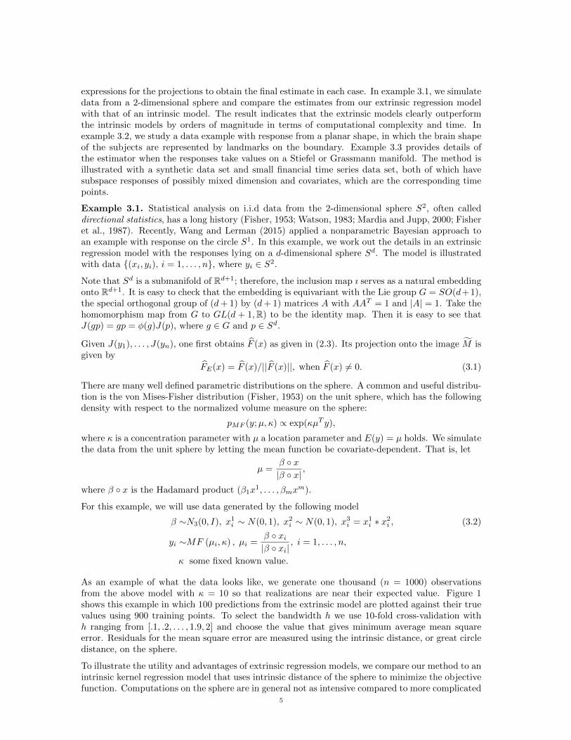
As an example of what the data looks like, we generate one thousand (n = 1000) observationsfrom the above model with κ = 10 so that realizations are near their expected value. Figure 1shows this example in which 100 predictions from the extrinsic model are plotted against their truevalues using 900 training points. To select the bandwidth h we use 10-fold cross-validation withh ranging from [.1, .2, . . . , 1.9, 2] and choose the value that gives minimum average mean squareerror. Residuals for the mean square error are measured using the intrinsic distance, or great circledistance, on the sphere.
To illustrate the utility and advantages of extrinsic regression models, we compare our method to anintrinsic kernel regression model that uses intrinsic distance of the sphere to minimize the objectivefunction. Computations on the sphere are in general not as intensive compared to more complicated
5
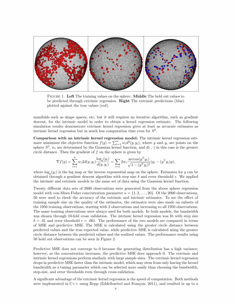
Figure 1. Left The training values on the sphere. Middle The held out values tobe predicted through extrinsic regression. Right The extrinsic predictions (blue)plotted against the true values (red).
manifolds such as shape spaces, etc, but it still requires an iterative algorithm, such as gradientdescent, for the intrinsic model in order to obtain a kernel regression estimate. The followingsimulation results demonstrate extrinsic kernel regression gives at least as accurate estimates asintrinsic kernel regression but in much less computation time even for S2.
Comparison with an intrinsic kernel regression model: The intrinsic kernel regression esti-mate minimizes the objective function f(y) =
∑ni=1 wid
2(y, yi), where y and yi are points on thesphere S2, wi are determined by the Gaussian kernel function, and d(·, ·) in this case is the greatercircle distance. Then the gradient of f on the sphere is given by
∇f(y) =
n∑i=1
wi2d(y, yi)logy(yi)
d(y, yi)=∑i=1
2wiarccos(yT yi)√
1− (yT yi)2(yi − (yT yi)y),
where logy(yi) is the log map or the inverse exponential map on the sphere. Estimates for y can beobtained through a gradient descent algorithm with step size δ and error threshold ε. We appliedthe intrinsic and extrinsic models to the same set of data using the Gaussian kernel function.
Twenty different data sets of 2000 observations were generated from the above sphere regressionmodel with von-Mises Fisher concentration parameter κ = {1, 2, . . . , 20}. Of the 2000 observations,50 were used to check the accuracy of the extrinsic and intrinsic estimates. To see the effect oftraining sample size on the quality of the estimates, the estimates were also made on subsets ofthe 1950 training observations, starting with 2 observations and increasing to all 1950 observations.The same training observations were always used for both models. In both models, the bandwidthwas chosen through 10-fold cross validation. The intrinsic kernel regression was fit with step sizeδ = .01 and error threshold ε = .001. The performance of the two models are compared in termsof MSE and predictive MSE. The MSE is calculated using the greater circle distance betweenpredicted values and the true expected value, while predictive MSE is calculated using the greatercircle distance between the predicted values and the realized values. The performance results using50 hold out observations can be seen in Figure 2.
Predictive MSE does not converge to 0 because the generating distribution has a high variance;however, as the concentration increases, the predictive MSE does approach 0. The extrinsic andintrinsic kernel regressions perform similarly with large sample sizes. The extrinsic kernel regressiondrops in predictive MSE faster than the intrinsic model, which may stem from only having the kernelbandwidth as a tuning parameter which can be selected more easily than choosing the bandwidth,step-size, and error thresholds even through cross-validation.
A significant advantage of the extrinsic kernel regression is the speed of computation. Both methodswere implemented in C++ using Rcpp (Eddelbuettel and Francois, 2011), and resulted in up to a
6
Figure 2. The performance of extrinsic and intrinsic regression models on 50 testobservations from sphere regression models with concentration parameters from 1to 20. Each color corresponds to a concentration parameter. The extrinsic andintrinsic models have similar performance in predictive MSE with low concentrationparameters. However in terms of MSE, the extrinsic model appears to performbetter with lower sample sizes even with lower concentration parameters.
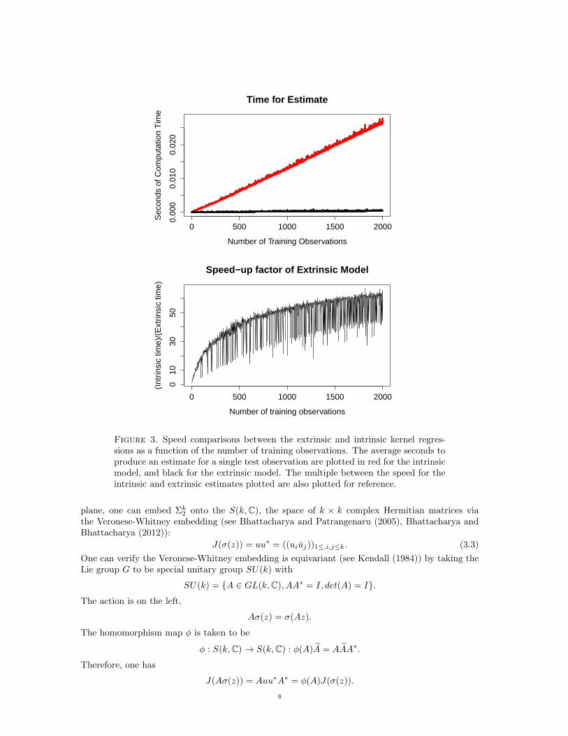
60× improvement in speed in making a single prediction using all of the training observations. Forspeed comparisons, a single prediction was made given the same number of test observations, andthe time to produce the estimate was recorded. Each of these trials was done five times, and wecompare the mean time to producing the estimate in Figure 3.
Note that the same kernel weights are computed in both algorithms, so the difference is attributableto the gradient descent versus extrinsic optimization procedures. Since the speed comparisons weredone for computing a single prediction and the difference is due almost entirely to the gradientdescent steps, making multiple predictions results in an even more favorable comparison for theextrinsic model. This experiment shows that the extrinsic kernel regression applied to sphere dataperforms at least as well on prediction and can be computed significantly faster.
Example 3.2. We now consider an example with planar shape responses. Planar shapes areone of the most important classes of landmark based shapes spaces. Such spaces were definedby Kendall (1977) and Kendall (1984) with pioneering work by Bookstein (1978) motivated fromapplications on biological shapes. We now describe the geometry of the space which will be usedin obtaining regression estimates for our model. Let z = (z1, . . . , zk) with z1, . . . , zk ∈ R2 be a set
of k landmarks. Let < z >= (z, . . . , z) where z =∑ki=1 zi/k. Denote u =
z− < z >
||z− < z > ||which can
be viewed as an element on the sphere S2k−3, which is called the pre-shape. The planar shape Σk2can now be represented as the quotient of the pre-shape under the group action by SO(2), the 2by 2 special orthogonal group. That is, Σk2 = S2k−2−1/SO(2). Σk2 can be shown to be equivalentto the complex projective space CPk−2. Therefore, a point on the planar shape can be identifiedas the orbit or equivalent of z which we denote by σ(z). Viewing z as elements in the complex
7
0 500 1000 1500 2000
0.00
00.
010
0.02
0
Time for Estimate
Number of Training Observations
Sec
onds
of C
ompu
tatio
n T
ime
0 500 1000 1500 2000
010
3050
Speed−up factor of Extrinsic Model
Number of training observations
(Int
rinsi
c tim
e)/(
Ext
rinsi
c tim
e)
Figure 3. Speed comparisons between the extrinsic and intrinsic kernel regres-sions as a function of the number of training observations. The average seconds toproduce an estimate for a single test observation are plotted in red for the intrinsicmodel, and black for the extrinsic model. The multiple between the speed for theintrinsic and extrinsic estimates plotted are also plotted for reference.
plane, one can embed Σk2 onto the S(k,C), the space of k × k complex Hermitian matrices viathe Veronese-Whitney embedding (see Bhattacharya and Patrangenaru (2005), Bhattacharya andBhattacharya (2012)):
J(σ(z)) = uu∗ = ((uiuj))1≤,i,j≤k. (3.3)
One can verify the Veronese-Whitney embedding is equivariant (see Kendall (1984)) by taking theLie group G to be special unitary group SU(k) with
SU(k) = {A ∈ GL(k,C), AA∗ = I, det(A) = I}.The action is on the left,
Aσ(z) = σ(Az).
The homomorphism map φ is taken to be
φ : S(k,C)→ S(k,C) : φ(A)A = AAA∗.
Therefore, one has
J(Aσ(z)) = Auu∗A∗ = φ(A)J(σ(z)).
8
We now describe the projection after F (x) is given by (2.3), where J(yi) (i = 1, . . . , n) are obtainedusing the equivariant embedding given in (3.3). Letting vT be the eigenvector corresponding to
largest eigenvalue of F (x), by a careful calculation, one can show that the projection of F (x) isgiven by
PJ(M)
(F (x)
)= vT v.
Therefore, the extrinsic kernel regression estimate is given by
FE(x) = J−1(vT v). (3.4)
Corpus Callosum (CC) data set: We study ADHD-200 dataset 1 in which the shape contourof the brain Corpus Callosum are recorded for each subject along with variables such as gender,age, and ADHD diagnosis. The subjects consist of patients who are diagnosed with ADHD. 50landmarks were placed outlining the CC shape for 647 patients for the ADHD-200 dataset. Theage of the patients range from 7 to 21 years old, with 404 typically developing children and 243individuals diagnosed with some form of ADHD. The original data set differentiates between typesof ADHD diagnoses, and we simplify the problem of choosing a kernel by using a binary responsefor an ADHD diagnosis.
According to the findings in Huang et al. (2015), there is not a significant effect of gender onthe area of different segments of the CC; however diagnosis and the interaction between diagnosisand age were found to be statistically significant (p < .01). With knowledge of these results, weperformed the extrinsic kernel regression method for the CC planar shape response using diagnosis,x1, and age, x2, for covariates. The choice of kernel between two sets of covariates x1 = (x11, x
21)
and x2 = (x12, x22) is
KH(x1, x2) =
{exp
(− (x2
1−x22)
2
h
)/h2 if x11 ≡ x12
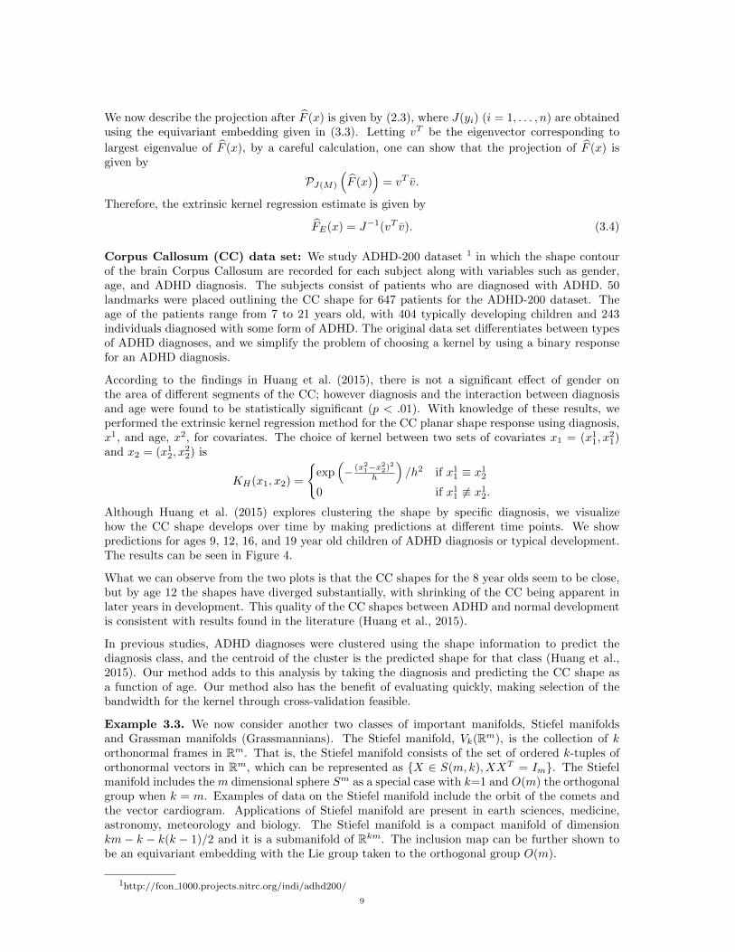
0 if x11 6≡ x12.Although Huang et al. (2015) explores clustering the shape by specific diagnosis, we visualizehow the CC shape develops over time by making predictions at different time points. We showpredictions for ages 9, 12, 16, and 19 year old children of ADHD diagnosis or typical development.The results can be seen in Figure 4.
What we can observe from the two plots is that the CC shapes for the 8 year olds seem to be close,but by age 12 the shapes have diverged substantially, with shrinking of the CC being apparent inlater years in development. This quality of the CC shapes between ADHD and normal developmentis consistent with results found in the literature (Huang et al., 2015).
In previous studies, ADHD diagnoses were clustered using the shape information to predict thediagnosis class, and the centroid of the cluster is the predicted shape for that class (Huang et al.,2015). Our method adds to this analysis by taking the diagnosis and predicting the CC shape asa function of age. Our method also has the benefit of evaluating quickly, making selection of thebandwidth for the kernel through cross-validation feasible.
Example 3.3. We now consider another two classes of important manifolds, Stiefel manifoldsand Grassman manifolds (Grassmannians). The Stiefel manifold, Vk(Rm), is the collection of korthonormal frames in Rm. That is, the Stiefel manifold consists of the set of ordered k-tuples oforthonormal vectors in Rm, which can be represented as {X ∈ S(m, k), XXT = Im}. The Stiefelmanifold includes the m dimensional sphere Sm as a special case with k=1 and O(m) the orthogonalgroup when k = m. Examples of data on the Stiefel manifold include the orbit of the comets andthe vector cardiogram. Applications of Stiefel manifold are present in earth sciences, medicine,astronomy, meteorology and biology. The Stiefel manifold is a compact manifold of dimensionkm − k − k(k − 1)/2 and it is a submanifold of Rkm. The inclusion map can be further shown tobe an equivariant embedding with the Lie group taken to the orthogonal group O(m).
1http://fcon 1000.projects.nitrc.org/indi/adhd200/
9
−0.10 −0.05 0.00 0.05 0.10
−0.
20.
00.
2
CC Shape age 9
−0.10 −0.05 0.00 0.05 0.10
−0.
20.
00.
2
CC Shape Age 12
−0.10 −0.05 0.00 0.05 0.10
−0.
20.
00.
2
CC Shape age 16
−0.10 −0.05 0.00 0.05 0.10
−0.
20.
00.
2
CC Shape age 19
Figure 4. Predicted CC shape for children ages 9, 12, 16, and 19. The black shapecorresponds to typically developing children, while the red shape corresponds tochildren diagnosed with ADHD. Kernel regression allows us to visualize how CCshape changes through development. Here sections of CC appear smaller in ADHDdiagnoses than in normal development.
Given F (x) obtained by kernel regression after embedding the points y1, . . . , yn on the Stiefel
manifold to the Euclidean space Rkm, the next step is to obtain the projection of F (x) onto
M = J(M). We first make an orthogonal decomposition of F (x) by letting F (x) = US, where
U ∈ Vk,m, which can be viewed as the orientation of F (x) and S is positive semi-definite, which
has the same rank as F (x). Then the projection of F (x) (or projection set) is given by
PM (F (x)) = {U ∈ Vk,m : F (x) = U(F (x)T F (x))1/2}.
See Theorem 10.2 in Bhattacharya and Bhattacharya (2012) for a proof of the results. Then the
projection is unique, that is, the above set is a singleton if and only if F (x) is of full rank.
The Grassmann manifold or the Grassmannian Grk(Rm) is the space of all the subspaces of a fixeddimension k whose basis elements are vectors in Rm, which is closely related to the Stiefel manifoldVk,m. Recall a subspace can be viewed as the span of an orthonormal basis. Let v = {v1, . . . , vk}be such an orthonormal basis for a subspace on the Grassmannian. Note that the order of thevector does not matter unlike in the case of Stiefel manifold. For any two elements on the Stiefelmanifold whose span corresponds to the same subspace, there exists an orthogonal transformation(mapped by a orthogonal matrix in O(k)) between the two orthonormal frames. These two pointswill be identified as the same point on the Grassman manifold. Therefore, the Grassmannian can beviewed as the collection of the equivalent classes on the Stiefel manifold, i.e., a quotient space under
10
the group action of O(k), the k by k orthogonal group. Then one has Grk(Rm) = Vk(Rm)/O(k).There are many applications of Grassmann manifolds, in which the subspaces are the basic elementin signal processing, machine learning and so on.
The equivariant embedding for Grk(Rm) also exists (Chikuse, 2003). Let X ∈ Vk,m be a represen-tative element of the equivalent classes in Grk(Rm) = Vk(Rm)/O(k). So an element in the quotientspace can be represented by the orbit σ(X) = XR where R ∈ O(k). Then an embedding can begiven by
J(σ(X)) = XXT .
The collection of XXT forms a subspace of Rm2
. We now verify that J is an equivariant embeddingunder the group action of G = O(m). Letting g ∈ G = O(m), one has J(gX) = gXXT gT =φ(g)J(X), where the map φ(g) = g acts on the image J(X) by the conjugation map. That is,φ(g)J(X) = gXXT gT .
Given the estimate F (x), the next step is to derive the projection of F (x) onto M = J(M). Since
all XXT form a subspace, one can use the following procedure to calculate the map from F (x) tothe Grassmann manifold by finding an orthonormal basis for the image. This algorithm is a specialcase of the projection via Conway embedding (St. Thomas et al., 2014).
(1) Find the eigendecomposition F (x) = QΛQ−1
(2) Take the k eigenvectors corresponding to the top k eigenvalues in Λ as an orthonormal basis
for FE(x), Q[1:k,].
We now consider two illustrative examples, one synthetic and one from a financial time series, forextrinsic kernel regression with subspace response variables. The technique is unique comparedto other subspace regression techniques because the extrinsic distance offers a well defined andprincipled distance between responses of different dimension. This prevents having to constrain theresponses to be a fixed dimension or hard coding a heuristic distance between subspaces of differentdimension into the distance function.
We now consider a synthetic example in which the predictors are the time points and the responsesare points on the Grassmann manifold. Since we represent subspaces with draws from the Stiefelmanifold, we draw orthonormal bases from the Matrix von Mises-Fisher distribution as their rep-resentation. We generate N draws from the following process with concentration parameter κ, inwhich the first n1 draws are of dimension 4 and the last n2 draws are of dimension 5,
for 1 ≤ t ≤ N doDraw X ∼MN(0, Im, I5)µ[,1] := t+X[,1], µ[,2] := t−X[,2], µ[,3] := t2 +X[,3], µ[,4] := tX[,4]
if t > n1 thenµ[,5] := t+ tX[,5]
end ifYt := vMF(κM)
end for
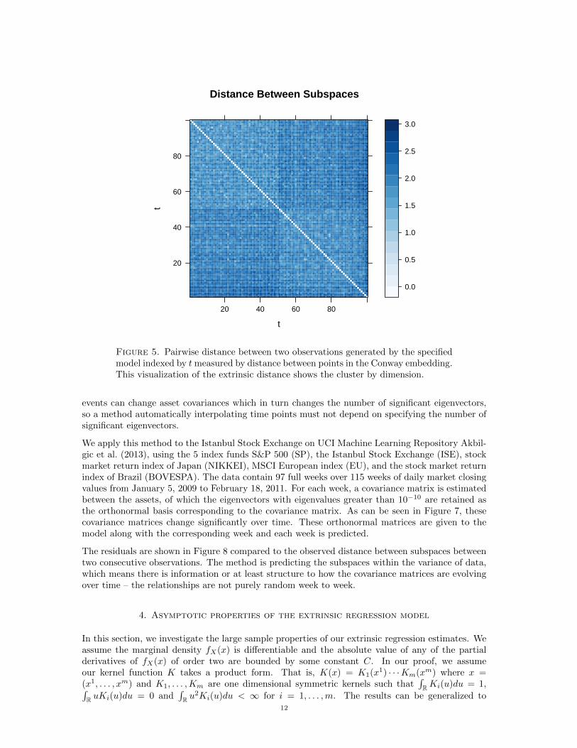
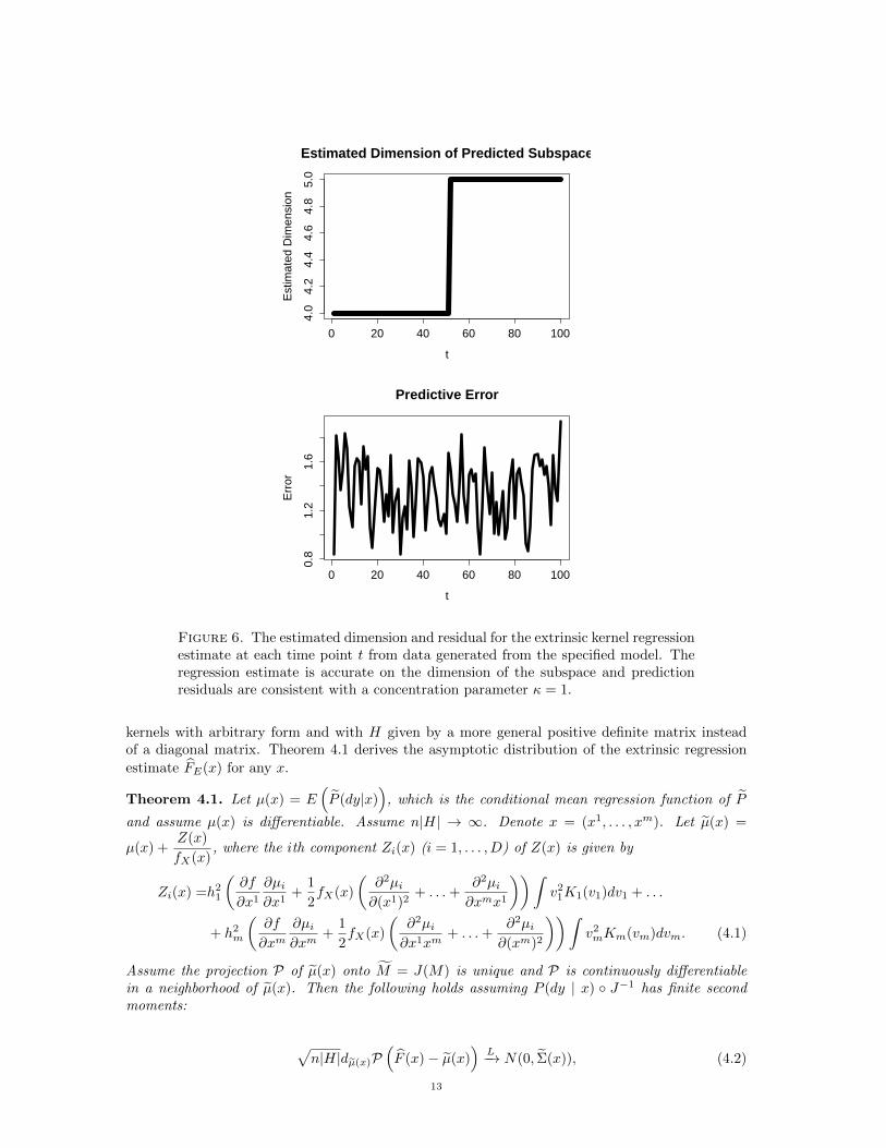
Here the only covariate associated with Yt is t. With a concentration of κ = 1, and n1 = n2 = 50,we generate much noisier data than before, and are able to correctly predict the dimension ofthe subspace at each time point. When examining the pairwise distance between the realizationsin Figure 5, it is clear that the extrinsic distance distinguishes between dimensions and does notrequire any specification of the dimension. The predicted dimension at each time point and theresiduals are plotted in Figure 6.
The key advantage of this method is not requiring any constraints on the dimension of the input oroutput subspaces. This is important in some examples, such as high dimensional time series analysiswith data such as high frequency trading where the analysis usually culminates in analyzing prin-cipal components, or eigenvectors of the large covariance matrix estimated between assets. Market
11
Distance Between Subspaces
t
t
20
40
60
80
20 40 60 80
0.0
0.5
1.0
1.5
2.0
2.5
3.0
Figure 5. Pairwise distance between two observations generated by the specifiedmodel indexed by tmeasured by distance between points in the Conway embedding.This visualization of the extrinsic distance shows the cluster by dimension.
events can change asset covariances which in turn changes the number of significant eigenvectors,so a method automatically interpolating time points must not depend on specifying the number ofsignificant eigenvectors.
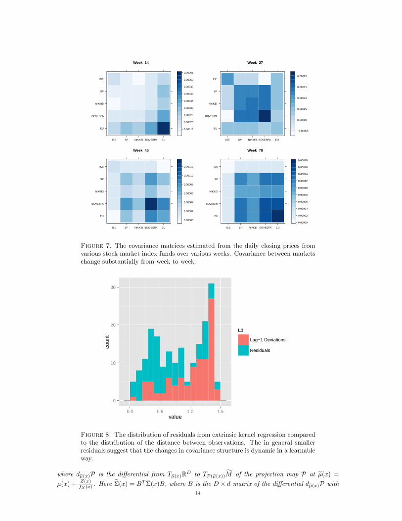
We apply this method to the Istanbul Stock Exchange on UCI Machine Learning Repository Akbil-gic et al. (2013), using the 5 index funds S&P 500 (SP), the Istanbul Stock Exchange (ISE), stockmarket return index of Japan (NIKKEI), MSCI European index (EU), and the stock market returnindex of Brazil (BOVESPA). The data contain 97 full weeks over 115 weeks of daily market closingvalues from January 5, 2009 to February 18, 2011. For each week, a covariance matrix is estimatedbetween the assets, of which the eigenvectors with eigenvalues greater than 10−10 are retained asthe orthonormal basis corresponding to the covariance matrix. As can be seen in Figure 7, thesecovariance matrices change significantly over time. These orthonormal matrices are given to themodel along with the corresponding week and each week is predicted.
The residuals are shown in Figure 8 compared to the observed distance between subspaces betweentwo consecutive observations. The method is predicting the subspaces within the variance of data,which means there is information or at least structure to how the covariance matrices are evolvingover time – the relationships are not purely random week to week.
4. Asymptotic properties of the extrinsic regression model
In this section, we investigate the large sample properties of our extrinsic regression estimates. Weassume the marginal density fX(x) is differentiable and the absolute value of any of the partialderivatives of fX(x) of order two are bounded by some constant C. In our proof, we assumeour kernel function K takes a product form. That is, K(x) = K1(x1) · · ·Km(xm) where x =(x1, . . . , xm) and K1, . . . ,Km are one dimensional symmetric kernels such that
∫RKi(u)du = 1,∫
R uKi(u)du = 0 and∫R u
2Ki(u)du < ∞ for i = 1, . . . ,m. The results can be generalized to12
0 20 40 60 80 100
4.0
4.2
4.4
4.6
4.8
5.0
Estimated Dimension of Predicted Subspace
t
Est
imat
ed D
imen
sion
0 20 40 60 80 100
0.8
1.2
1.6
Predictive Error
t
Err
or
Figure 6. The estimated dimension and residual for the extrinsic kernel regressionestimate at each time point t from data generated from the specified model. Theregression estimate is accurate on the dimension of the subspace and predictionresiduals are consistent with a concentration parameter κ = 1.
kernels with arbitrary form and with H given by a more general positive definite matrix insteadof a diagonal matrix. Theorem 4.1 derives the asymptotic distribution of the extrinsic regression
estimate FE(x) for any x.
Theorem 4.1. Let µ(x) = E(P (dy|x)
), which is the conditional mean regression function of P
and assume µ(x) is differentiable. Assume n|H| → ∞. Denote x = (x1, . . . , xm). Let µ(x) =
µ(x) +Z(x)
fX(x), where the ith component Zi(x) (i = 1, . . . , D) of Z(x) is given by
Zi(x) =h21
(∂f
∂x1∂µi∂x1
+1
2fX(x)
(∂2µi∂(x1)2
+ . . .+∂2µi∂xmx1
))∫v21K1(v1)dv1 + . . .
+ h2m
(∂f
∂xm∂µi∂xm
+1
2fX(x)
(∂2µi∂x1xm
+ . . .+∂2µi∂(xm)2
))∫v2mKm(vm)dvm. (4.1)
Assume the projection P of µ(x) onto M = J(M) is unique and P is continuously differentiablein a neighborhood of µ(x). Then the following holds assuming P (dy | x) ◦ J−1 has finite secondmoments:
√n|H|dµ(x)P
(F (x)− µ(x)
)L−→ N(0, Σ(x)), (4.2)
13
Week 14
EU
BOVESPA
NIKKEI
SP
ISE
ISE SP NIKKEI BOVESPA EU
0.00015
0.00020
0.00025
0.00030
0.00035
0.00040
0.00045
0.00050
0.00055
Week 27
EU
BOVESPA
NIKKEI
SP
ISE
ISE SP NIKKEI BOVESPA EU
−0.00005
0.00000
0.00005
0.00010
0.00015
0.00020
Week 46
EU
BOVESPA
NIKKEI
SP
ISE
ISE SP NIKKEI BOVESPA EU
0.00000
0.00002
0.00004
0.00006
0.00008
0.00010
0.00012
Week 78
EU
BOVESPA
NIKKEI
SP
ISE
ISE SP NIKKEI BOVESPA EU
0.00000
0.00002
0.00004
0.00006
0.00008
0.00010
0.00012
0.00014
0.00016
0.00018
Figure 7. The covariance matrices estimated from the daily closing prices fromvarious stock market index funds over various weeks. Covariance between marketschange substantially from week to week.
0
10
20
30
0.0 0.5 1.0 1.5value
coun
t
L1
Lag−1 Deviations
Residuals
Figure 8. The distribution of residuals from extrinsic kernel regression comparedto the distribution of the distance between observations. The in general smallerresiduals suggest that the changes in covariance structure is dynamic in a learnableway.
where dµ(x)P is the differential from Tµ(x)RD to TP(µ(x))M of the projection map P at µ(x) =
µ(x) + Z(x)fX(x) . Here Σ(x) = BT Σ(x)B, where B is the D × d matrix of the differential dµ(x)P with
14
respect to given orthonormal bases of Tµ(x)RD and TP(µ(x))M , and the (j, k)th entry of Σ(x) isgiven by (5.13) with
Σjk =σ(Jj(y), Jk(y))
∫K(v)2dv
fX(x), (4.3)
where σ(Jj(y), Jk(y)) = Cov(Jj , Jk), and Jj is the jth element of J(y). HereL−→ indicates conver-
gence in distribution.
Corollary 4.2 is on the mean integrated squared error of the estimates.
Corollary 4.2. Assuming the same conditions of Theorem 4.1 and the covariate space is bounded,
the mean integrated squared error of FE(x) is of the order O(n−4/(m+4)), with the choice of hi’s(i = 1, . . . ,m) to be of the same order, that is, of O(n−1/(m+4)).
Remark 4.1. Note that in nonparametric regression with both predictors (m-dimensional) andresponses in the Euclidean space, the optimal order of the mean integrated squared error isO(n−4/(m+4)) under the assumption that the true regression function has bounded second de-rivative. Our method achieves the same rates. However, whether such rates are minimax in thecontext of manifold valued response is not known.
Theorem 4.3 shows some results on uniform convergence rates of the estimator.
Theorem 4.3. Assume the covariate space x ∈ X ⊂ Rm is compact and P has continuous firstderivative. Then
supx∈X‖dµ(x)P
(F (x)− E(F (x))
)‖ = Op
(log1/2 n/
√n|H|
). (4.4)
As pointed out in Remark 2.3, it is ideal in many cases to fit a higher order (say pth order) localpolynomial model in estimating µ(x) before projecting back onto the image of the manifold. Suchestimates are more appealing especially when F (x) is more curved over a neighborhood of x. Onecan show that similar results as those of Theorem 4.1 hold, though with much more involvedargument.
We now give details of such estimators and their asymptotic distributions are derived in Theorem
4.4. Recall F (x) = E (P (dy | x)) and µ(x) = E(P (dy | x)
)and J(y1), . . . , J(yn) are the points
on M = J(M) after embedding J . We first obtain an estimate F (x) of µ(x) using pth order local
polynomials estimation. The intermediate estimate F (x) is then projected back to M serving asthe ultimate estimate of F (x). The general framework is given as follows:
{βjk(x)}0≤|k|≤p, 1≤j≤D (4.5)
= argmin{βj
k(x)}0≤|k|≤p, 1≤j≤D
n∑i=1
(∥∥J(yi)−( ∑0≤|k|≤p
β1k(x)(xi − x)|k|, . . . ,
∑0≤|k|≤p
βDk (x)(xi − x)|k|)T∥∥2
×KH(xi − x)). (4.6)
Some of the notation used in (4.5) are given as follows:
k = (k1, . . . , km), |k| =m∑l=1
kl, |k| ∈ {0, . . . , p},
k! = k1!× . . .× km!, xk = (x1)k1 × . . .× (xm)km∑0≤|k|≤p
=
p∑j=0
j∑k1=0
. . .
j∑km=0
|k|=k1+...+km=j
.
15
When k=0,(β10, . . . , β
D0
)Tcorresponds to the kernel estimator, which is the same as the estimator
given in (2.3). When p = 1,(β1k=0, . . . , β
Dk=0
)Tcoincides with the estimator β0 in (2.6).
Finally, we have
F (x) = β0(x) =(β1k=0, . . . , β
Dk=0
)T, (4.7)
FE(x) = J−1(P(F (x))
)= J−1
(argminq∈M
||q − F (x)||
). (4.8)
Theorem 4.4 derives the asymptotic distribution of FE(x), with F (x) obtained using pth orderpolynomials local regression of J(y1), . . . , J(yn) given in (4.7).
Theorem 4.4. Let FE(x) be given in (4.8). Assume the (p + 2)th moment of the kernel functionK(x) exists and µ(x) is (p+2)th order differentiable in a neighborhood of x = (x1, . . . , xm). Assume
the projection P of µ(x) onto M = J(M) is unique and P is continuously differentiable in aneighborhood of µ(x), where µ(x) = µ(x)+ Bias(x), with Bias(x) given in (5.23). If P (dy | x)◦J−1has finite second moments, then we have:
√n|H|dµ(x)P
(F (x)− µ(x)
)L−→ N(0, Σ(x)), (4.9)
where dµ(x)P is the differential from Tµ(x)RD to TPµ(x)M of the projection map P at µ(x). Here
Σ(x) = BT Σ(x)B, where B is the D × d matrix of the differential dµ(x)P with respect to given
orthonormal basis of tangent space Tµ(x)RD and tangent space TPµ(x)M and the jkth entry of Σ(x)
is given by (5.26). HereL−→ indicates convergence in distribution.
Remark 4.2. Note that the order of the bias term Bias(x) (given in (5.23)) differs when p is even(see (5.21)) and when p is odd (see (5.22)).
5. Conclusion
We have proposed an extrinsic regression framework for modeling data with manifold valued re-sponses and shown desirable asymptotic properties of the resulting estimators. We applied thisframework to a variety of applications, such as responses restricted to the sphere, shape spaces, andlinear subspaces. The principle motivating this framework is that kernel regression and Riemanniangeometry both rely on locally Euclidean structures. This property allows us to construct inexpen-sive estimators without loss of predictive accuracy as demonstrated by the asymptotic behavior ofthe mean integrated square error, and also the empirical results. Empirical results even suggestthat the extrinsic estimators may perform better due to their reduced complexity and ease of op-timizing tuning parameters such as kernel bandwidth. Future work may also use this principle toguide sampling methodology when trying to sample parameters from a manifold or optimizing anEM-algorithm, where it may be computationally or mathematically difficult to restrict intermediatesteps to the manifold.
Appendix
Proof of Theorem 4.1. Recall
F (x) =1n
∑ni=1 J(yi)KH(xi − x)
1n
∑ni=1KH(xi − x)
.
16
Denote the denominator of F (x) as
f(x) =1
n
n∑i=1
KH(xi − x) =1
n | H |
n∑i=1
K(xi − x).
It is standard to show
f(x)P−→ fX(x) (5.1)
whereP−→ indicates convergence in probability. For the numerator term of F (x), one has
E
(1
n
n∑i=1
J(yi)KH(xi − x))
)=
1
n
n∑i=1
E (J(yi)KH(xi − x)))
=1
n
n∑i=1
∫E (J(yi)KH(xi − x)) | xi) fX(xi)dxi
=1
n
n∑i=1
∫µ(xi)KH(xi − x))fX(xi)dxi
=
∫µ(x)KH(x− x))fX(x)dx.
Noting that µ(x) = (µ1(x), . . . , µD(x))′ ∈ RD, we slightly abuse the integral notation above meaningthat the jth entry of E
(n−1
∑ni=1 J(yi)KH(xi − x))
)is given by∫
µj(x)KH(x− x))fX(x)dx.
Letting v = H−1(x− x) by changing of variables, the above equations become
E
(1
n
n∑i=1
J(yi)KH(xi − x))
)=
∫µ(x+Hv)K(v)fX(x+Hv)dv.
By the multivariate Taylor expansion,
fX(x+Hv) = fX(x) + (5f) · (Hv) +R, (5.2)
where 5f is the gradient of f and R is the remainder term of the expansion. The remainder R canbe shown to be bounded above by
R ≤ C
2‖Hv‖2, ‖Hv‖ = |h1v1|+ . . . |hmvm|.
Note that µ(x+Hv) is a multivariate map valued in RD. We can make second order multivariateTaylor expansions for µ(x + Hv) = (µ1(x + Hv), . . . , µD(x + Hv))′ at each of its entries µi fori = 1, . . . , D. We have
µ(x+Hv) = µ(x) +A(Hv) + V +R, (5.3)
where A is a D ×m matrix whose ith row is given by the gradient of µi evaluated at x. V is aD-dimensional vector, whose ith term is given by 1
2 (Hv)tTi(Hv), where Ti is the Hessian matrix of17
µi(x) and R is the remainder vector. Thus,
E
(1
n
n∑i=1
J(yi)KH(xi − x))
)(5.4)
≈∫
((fX(x) + (5f) · (Hv))K(v)(µ(x) +A(Hv) + V )) dv
= fX(x)µ(x) + fX(x)
∫K(v)A(Hv)dv + fX(x)
∫K(v)V dv (5.5)
+ µ(x)
∫(5f) · (Hv)K(v)dv +
∫(5f) · (Hv)K(v)A(Hv)dv +
∫(5f) · (Hv)K(v)V dv. (5.6)
By the property of the kernel function, we have∫K(u)udu = 0; therefore the second term of
equation (5.5) is zero by simple algebra. To evaluate the third term of equation (5.5), we firstcalculate for
∫K(v)V dv. From here onward until the end of the proof, we denote x = (x1, . . . , xm)
where xi is the ith coordinate of x. Note that the ith term of V (i = 1, . . . , D) is given by1
2(Hv)tTi(Hv), where Ti is the Hessian matrix of µi, which is precisely
1
2h21v
21
(∂2µi∂(x1)2
+ . . .+∂2µi∂xmx1
)+ . . .+
1
2h2mv
2m
(∂2µi∂x1xm
+ . . .+∂2µi∂(xm)2
).
Therefore, the ith entry of the third term of equation (5.5) is given by
Ui =1
2fX(x)
(h21
(∂2µi∂(x1)2
+ . . .+∂2µi∂xmx1
)∫v21K1(v1)dv1 + . . . (5.7)
+ h2m
(∂2µi∂x1xm
+ . . .+∂2µi∂(xm)2
)∫v2mKm(vm)dvm
).
The first term of equation (5.6) is given by
µ(x)
∫(5f) · (Hv)K(v)dv =
∫ (h1v1
∂f
∂x1+ . . .+ hmvm
∂f
∂xm
)K(v)dv = 0.
The ith entry of the second term of equation (5.6) is given by
h21∂f
∂x1∂µi∂x1
∫v21K1(v1)dv1 + . . .+ h2m
∂f
∂xm∂µi∂xm
∫v2mKm(vm)dvm. (5.8)
The third term of equation (5.6) can be shown to be zero, since odd moments of symmetric kernelsare 0. Therefore, we have
E
(1
n
n∑i=1
J(yi)KH(xi − x))
)≈ fX(x)µ(x) + Z, (5.9)
where the ith coordinate of Z is
Zi =h21
{∂f
∂x1∂µi∂x1
+1
2fX(x)
(∂2µi∂(x1)2
+ . . .+∂2µi∂xmx1
)}∫v21K1(v1)dv1
+ . . .
+ h2m
{∂f
∂xm∂µi∂xm
+1
2fX(x)
(∂2µi∂x1xm
+ . . .+∂2µi∂(xm)2
)}∫v2mKm(vm)dvm (5.10)
combining equations (5.7) and (5.8). The reminder term of (5.2) is of order o(max{h1, . . . , hm})and each entry of the remainder vector in (5.3) is of order o(max{h21, . . . , h2m}).
We now look at the covariance matrix of n−1∑ni=1 J(yi)KH(xi − x)), which we denote by Σ(x).
Denote the jth entry (j = 1, . . . , D) of J(yi) as Jj(yi). Denote σ(yj , yk) as the conditional covariance18
between the ith entry and jth entry of y. We have
Σjk = E[( 1
n
n∑i=1
Jj(yi)KH(xi − x))− E
(1
n
n∑i=1
Jj(yi)KH(xi − x))
))(
1
n
n∑i=1
Jk(yi)KH(xi − x))− E
(1
n
n∑i=1
Jk(yi)KH(xi − x))
))]= E
[( 1
n
n∑i=1
(Jj(yi)KH(xi − x))−
∫µj(x)KH(x− x)fX(x)dx
))(
1
n
n∑i=1
(Jk(yi)KH(xi − x))−
∫µk(x)KH(x− x)fX(x)dx
))]=
1
n
∫E[(
Jj(y1)KH(x1 − x))−∫µj(x)KH(x− x)fX(x)dx
)(Jk(y1)KH(x1 − x))−
∫µk(x)KH(x− x)fX(x)dx
)| x1]fX(x1)dx1
=1
n
∫σ(Jj(y1)KH(x1 − x)), Jk(y1)KH(x1 − x))fX(x1)dx1
=1
n
∫KH(x1 − x))2σ(Jj(y1), Jk(y1))fX(x1)dx1.
By the change of variable v = H−1(x1 − x), the above equation becomes
Σjk =1
n|H|
∫K(v)2σ(Jj(yv), Jk(yv))fX(Hv + x)dv
=1
n|H|
∫K(v)2σ(Jj(yv), Jk(yv)) (fX(x) +5f · (Hv) + o(max{h1, . . . , hm})) dv
=1
n|H|
∫K(v)2σ(Jj(yv), Jk(yv))fX(x))dv + o
(1
n|H|
). (5.11)
By (5.1), (5.9) and (5.24), and applying central limit theorem and Slustky’s theorem, one has√n|H|
(F (x)− µ(x)
)L−→ N(0, Σ(x)), (5.12)
where µ(x) = µ(x) + ZfX(x) and the ith entry (i = 1, . . . , D) of Z is given by (5.10) and
Σjk =σ(Jj(yv), Jk(yv))
∫K(v)2dv
fX(x). (5.13)
One can show √n|H|
(FE(x)− P (µ(x))
)=√n|H|dµ(x)P
(F (x)− µ(x)
)+ oP (1).
Therefore, one has √n|H|dµ(x)P
(F (x)− µ(x)
)L−→ N(0, Σ(x)). (5.14)
Here Σ(x) = BT Σ(x)B, where B is the D×d matrix of the differential dµ(x)P with respect to given
orthonormal bases of Tµ(x)RD and TPµ(x)M .
�
Proof of Corollary 4.2. In choosing the optimal order of bandwidth, one can consider choosing(h1, . . . , hm) such that the mean integrated squared error is minimized. Note that
FE(x)− F (x) = Jacob(P)µ(x)
(F (x)− µ(x)
)+ op(1). (5.15)
19
Here Jacob(P) is the Jacobian matrix of the projection map P. One has
MISE(FE(x)) =
∫E‖FE(x)− F (x)‖2dx
=
∫E‖Jacob(P)µ(x)
(F (x)− µ(x)
)+ op(1)‖2dx
=
∫E
D∑i=1
D∑j=1
Pij(Fj(x)− µj(x)
)2
+ op(1)
dx
= O(1/n|H|) + . . .+O(1/n|H|) +O(h41) + . . .+O(h4m).
The last terms follow from Fatou’s lemma, and that the Jacobian map is differentiable at µ(x) forevery x. Therefore, if hi’s (i = 1, . . . ,m) are taken to be of the same order, that is, of O(n−1/(m+4)),
then one can obtain MISE(FE(x)) with an order of O(n−4/(m+4)). �
Proof of Theorem 4.3. Let B be the D × d matrix of the differential dµ(x)P with respect to given
orthonormal basis of tangent space Tµ(x)RD and tangent space TPµ(x)M . Given a canonical choice
of basis for tangent space Tµ(x)RD, one has the representation for
supx‖dµ(x)P
(F (x)− E(F (x))
)‖ = sup
x
√√√√√ d∑i=1
D∑j=1
BTij
(Fj(x)− E(Fj(x))
)2
. (5.16)
Note that the projection map is differentiable around the neighborhood of µ(x) and X is compact,so BTij(x) are bounded. Let Cij = supx∈X (BTij)
2(x) and C = maxCij . For each term note that, byCauchy-Schwarz inequality,
supx∈X
D∑j=1
(BTij
(Fj(x)− E
(Fj(x)
)))2
≤ supx
D∑j=1
(BTij)2(Fj(x)− E
(Fj(x)
))2(5.17)
≤ CD∑j=1
supx∈X
(Fj(x)− E
(Fj(x)
))2. (5.18)
By Theorem 2 in Hansen (2008), one can see that
supx∈X|(Fj(x)− E
(Fj(x)
))| = O(rn), (5.19)
where rn = log1/2 n/√n|H|. Then one has
supx∈X
d∑i=1
D∑j=1
(Bij
(Fj(x)− E
(Fj(x)
)))2
= O(r2n). (5.20)
Then one has
supx‖dµ(x)P
(F (x)− E(F (x))
)‖ = sup
x∈X
√√√√√ d∑i=1
D∑j=1
(Bij
(Fj(x)− E
(Fj(x)
)))2
= O(rn) = O(
log1/2 n/√n|H|
).
�
Proof of Theorem 4.4. Given the higher order smoothness assumption on µ(x), one can make higherorder approximations and using a local polynomials regression estimate would result in the reductionof bias term in estimating µ(x). The asymptotic distribution for multivariate local regression
20
estimator for Euclidean responses has been derived (Gu et al., 2014; Ruppert and Wand, 1994;Masry, 1996), and we leverage on some of their results in our proof.
Note that F (x) =(F1(x), . . . , FD(x)
)∈ RD. E(F (x)) =
(E(F1(x)), . . . , E(FD(x))
)Tand the
expectation taken in each component is with respect to the marginal distribution of P (dy|x). Thenby Theorem 1 of Gu et al. (2014), the following holds:
(1) If p is odd, then for j = 1, . . . , D
Biasj(F (x)) = E(Fj(x))− µj(x)
=(M−1p Bp+1H
(p+1)mjp+1(x)
)1, (5.21)
which is of order O(‖h‖p+1). Here (·)1 represents the first entry of the vector inside theparenthesis;
(2) If p is even, then for j = 1, . . . , D
Biasj(F (x)) = E(Fj(x))− µj(x) (5.22)
=
(m∑l=1
hlfl(x)
fX(x)
(M−1p Blp+1 −M−1p Ml
pM−1p Bp+1
)H(p+1)mj
p+1(x) +M−1p Bp+2H(p+2)mj
p+2(x)
)1
,
which is of order O(‖h‖p+2).
For any k ∈ {0, 1, . . . , p}. Let Nk =(k+m−1m−1
)and Np =
∑pk=0Nk. Here Mp is a Np × Np
matrix whose (i, j)th block (0 ≤ i, j ≤ p) is given by∫Rm u
i+jK(u)du and Mlp (l = 1, . . . ,m)
is a Np × Np matrix whose (i, j)th block (0 ≤ i, j ≤ p) is given by∫Rm ulu
i+jK(u)du. Bp+1 is
a Np × Np+1 matrix whose (i, p + 1)th (i = 1, . . . , p) block is given by∫Rm u
i+p+1K(u)du and
Blp+1 (l = 1, . . . ,m) is a Np × Np+1 matrix whose (i, p + 1)th (i = 1, . . . , p) block is given by∫Rm ulu
i+p+1K(u)du. We have H(p+1) = Diag{hp+11 , . . . , hp+1
m }. fl(x) =∂fX(x)
∂xland mj
p+1(x)
(j = 1, . . . , D) is the vector of all the p + 1 order partial derivative of µj(x), that is, mjp+1(x) =(
∂µp+1j (x)
∂(x1)p+1,∂µp+1
j (x)
∂(x1)p∂(x2), . . . ,
∂µp+1j (x)
∂(xm)p+1
).
With Biasj(F (x)) (j = 1, . . . , D) given above, one has
Bias(x) = E(F (x)))− µ(x) =(
Bias1(F (x)), . . . ,BiasD(F (x)))T
. (5.23)
Although higher order polynomial regression results in the reduction in the order of bias with thehigher order smoothness assumptions on µ(x), the order and expression of the covariance remainsthe same. That is,
Σjk = Cov(Fj(x), Fk(x))
=1
n|H|fX(x)−1
∫K(v)2σ(Jj(yv), Jk(yv))dv + o
(1
n|H|
), (5.24)
where σ(Jj(yv), Jk(yv) is the covariance between Jj(yv) and Jk(yv).
Applying the central limit theorem, one has√n|H|
(F (x)− µ(x)− Bias(x)
)L−→ N(0, Σ(x)) (5.25)
where the jth (j = 1, . . . , D) entry of Bias(x) is given in (5.21) or (5.22) depending on p is odd oreven, and
Σjk =σ(Jj(yv), Jk(yv))
∫K(v)2dv
fX(x). (5.26)
21
Letting µ(x) = µ(x) + Bias(x), one has√n|H|
(FE(x)− P (µ(x))
)=√n|H|dµ(x)P
(F (x)− µ(x)
)+ oP (1).
Therefore by applying Slutsky’s theorem, one has√n|H|dµ(x)P
(F (x)− µ(x)
)L−→ N(0, Σ(x)). (5.27)
Here Σ(x) = BT Σ(x)B where B is the D×d matrix of the differential dµ(x)P with respect to given
orthonormal bases of the tangent space Tµ(x)RD and tangent space Tµ(x)M .
�
References
Akbilgic, O., Bozdogan, H., and Balaban, M. (2013). A novel Hybrid RBF Neural Networks modelas a forecaster. Statistics and Computing.
Alexander, A., Lee, J., Lazar, M., and Field, A. (2007). Diffusion tensor imaging of the brain.Neurotherapeutics, 4(3):316–329.
Bhattacharya, A. and Bhattacharya, R. (2012). Nonparametric Inference on Manifolds: WithApplications to Shape Spaces. IMS Monograph #2. Cambridge University Press.
Bhattacharya, A. and Dunson, D. B. (2010). Nonparametric Bayesian density estimation on man-ifolds with applications to planar shapes. Biometrika, 97(4):851–865.
Bhattacharya, R. and Lin, L. (2013). An omnibus CLT for Frechet means and nonparametricinference on non-Euclidean spaces. ArXiv eprint, 1306.5806.
Bhattacharya, R. N. and Patrangenaru, V. (2003). Large sample theory of intrinsic and extrinsicsample means on manifolds. Ann. Statist., 31:1–29.
Bhattacharya, R. N. and Patrangenaru, V. (2005). Large sample theory of intrinsic and extrinsicsample means on manifolds-ii. Ann. Statist., 33:1225–1259.
Bookstein, F. (1978). The Measurement of Biological Shape and Shape Change. Lecture Notes inBiomathematics, Springer, Berlin.
Cheng, M. and Wu, H. (2013). Local linear regression on manifolds and its geometric interpretation.Journal of the American Statistical Association, 108(504):1421–1434.
Chikuse, Y. (2003). Statistics on Special Manifolds, volume 174. Springer series: lecture notes instatistics.
Davis, B., Fletcher, P., Bullitt, E., and Joshi, S. (2007). Population shape regression from randomdesign data. In Computer Vision, 2007. ICCV 2007. IEEE 11th International Conference on,pages 1–7.
Downs, T., Liebman, J., and Mackay, W. (1971). Statistical methods for vectorcardiogram orien-tations. In Vectorcardiography 2: Proc. XIth International Symposium on Vectorcardiography (I.Hoffman, R.I. Hamby and E. Glassman, Eds.), pages 216–222. North-Holland, Amsterdam.
Eddelbuettel, D. and Francois, R. (2011). Rcpp: Seamless R and C++ integration. Journal ofStatistical Software, 40(8):1–18.
Fan, J. (1993). Local linear regression smoothers and their minimax efficiencies. Ann. Statist.,21(1):196–216.
Fan, J. and Gijbels, I. (1996). Local Polynomial Modelling and Its Applications. Chapman &Hall/CRC Monographs on Statistics & Applied Probability. Taylor & Francis.
Fisher, N., Lewis, T., and Embleton, B. (1987). Statistical Analysis of Spherical Data. CambridgeUni. Press, Cambridge.
Fisher, R. (1953). Dispersion on a sphere. Proc. Roy. Soc. London Ser. A, 217:295–305.Fletcher, T. (2011). Geodesic Regression on Riemannian Manifolds. In: MICCAI Workshop on
Mathematical Foundations of Computational Anatomy (MFCA), pages 75–86.Gu, J., Li, Q., and Yang, J.-C. (2014). Multivariate local polynomial kernel estimators: leading
bias and asymptotic distribution. Econometric Reviews. to appear.Hansen, B. E. (2008). Uniform convergence rates for kernel estimation with dependent data. Econo-
metric Theory, 24:726–748.22
Hinkle, J., Muralidharan, P., Fletcher, P., and Joshi, S. (2012). Polynomial regression on riemann-ian manifolds. In Fitzgibbon, A., Lazebnik, S., Perona, P., Sato, Y., and Schmid, C., editors,Computer Vision ECCV 2012, volume 7574 of Lecture Notes in Computer Science, pages 1–14.Springer Berlin Heidelberg.
Huang, C., Styner, M., and Zhu, H. (2015). Penalized mixtures of offset-normal shape factoranalyzers with application in clustering high-dimensional shape data. J. Amer. Statist. Assoc.,to appear.
Kendall, D. G. (1977). The diffusion of shape. Adv. Appl. Probab., 9:428–430.Kendall, D. G. (1984). Shape manifolds, procrustean metrics, and complex projective spaces. Bull.
of the London Math. Soc., 16:81–121.Le, H. and Barden, D. (2014). On the measure of the cut locus of a Frechet mean. Bulletin of the
London Mathematical Society, 46(4):698–708.Lin, L., Rao, V., and Dunson, D. B. (2013). Bayesian nonparametric inference on the Stiefel
manifold. ArXiv e-prints, 1311.0907.Mardia, K. and Jupp, P. (2000). Directional Statistics. Wiley, New York.Masry, E. (1996). Multivariate local polynomial regression for time series:uniform strong consistency
and rates. Journal of Time Series Analysis, 17(6):571–599.Pelletier, B. (2005). Kernel density estimation on riemannian manifolds. Statistics and Probability
Letters, 73(3):297 – 304.Ruppert, D. and Wand, M. P. (1994). Multivariate locally weighted least squares regression. The
Annals of Statistics, 22(3):1346–1370.Shi, X., Styner, M., Lieberman, J., Ibrahim, J. G., Lin, W., and Zhu, H. (2009). Intrinsic regression
models for manifold-valued data. Med Image Comput Comput Assist Interv., 12(2):192–199.St. Thomas, B., Lin, L., Lim, L.-H., and Mukherjee, S. (2014). Learning subspaces of different
dimension. ArXiv e-prints, 1404.6841.Wang, X. and Lerman, G. (2015). Nonparametric Bayesian Regression on Manifolds via Brownian
Motion. ArXiv e-prints.Watson, G. S. (1983). Statistics on Spheres, volume 6. University Arkansas Lecture Notes in the
Mathematical Sciences, Wiley, New York.Weiszfeld, E. (1937). Sur le point pour lequel la somme des distances de n points donnes est
minimum. Tohoku Mathematical Journal, 43:355–386.Yuan, Y., Zhu, H., Lin, W., and Marron, J. S. (2012). Local polynomial regression for symmetric
positive definite matrices. Journal of the Royal Statistical Society: Series B (Statistical Method-ology), 74(4):697–719.
E-mail address: [email protected]
Department of Statistics and Data Sciences, The University of Texas at Austin, Austin, TX.
E-mail address: [email protected]
Department of Statistical Science, Duke University, Durham, NC
E-mail address: [email protected]
UNC Gillings School of Global Public Health, The University of North Carolina at Chapel Hill, Chapel
Hill, NC
E-mail address: [email protected]
Department of Statistical Science, Duke University, Durham, NC
23