Extreme Weather Events, Mortality and Migration

Olivier Deschenes

University of California, Santa Barbara and NBER

Enrico Moretti

University of California, Berkeley and NBER

December 2007

Abstract. We estimate the effect of extreme weather on life expectancy in the US. Using high frequency mortality data, we find that both extreme heat and extreme cold result in immediate increases in mortality. However, the increase in mortality following extreme heat appears entirely driven by near-term displacement, while the increase in mortality following extreme cold is long lasting. The aggregate effect of cold on mortality is quantitatively large. We estimate that the number of annual deaths attributable to cold temperature is 14,380 or 0.8% of average annual deaths in the US during our sample period. Females account for two thirds of this excess mortality. We also find that males living in low-income areas have very high cold-mortality risks. Because the U.S. population has been moving from cold Northeastern states to the warmer Southwestern states, our findings have implications for understanding the causes of long-term increases in life expectancy. We calculate that every year, 4,600 deaths are delayed by changes in exposure to cold temperature induced by mobility. The longevity gains associated with long term trends in geographical mobility account for 4%-7% of the total gains in life expectancy experienced by the US population over the past 30 years. Thus mobility is an important but previously overlooked determinant of increased longevity in the United States.

We thank seminar participants at the Princeton University Industrial Relations Labor Lunch, UC Davis and UC Santa Cruz for useful suggestions. We also thank the editor and two anonymous referees for useful comments. Mariana Carrera and Paul McCathcart provided excellent research assistance.

1

1. Introduction

Through the twentieth century, the United States population has experienced an

unprecedented increase in life expectancy. The economic value of such increase is

enormous, exceeding, by some calculations, the value of the growth in all non-health

goods and services (Nordhaus, 2002). While the determinants of the increase in life

expectancy are numerous and complex, it appears that economic growth, public health

measures and especially science and technology were important determinants. Cutler,

Deaton and Lleras-Muney (2006) provide a recent survey of the importance of the

various determinants and their interplay.1

In this paper we focus on the relationship between weather and mortality in the

US. Specifically, we estimate the effect of episodes of extreme heat and extreme cold on

longevity. We use these estimates to provide new evidence on the underlying causes of

long-run increases in life expectancy experienced by the US population over the past

several decades.2

Extreme weather events generate enormous interest in the public. Each summer,

the popular press devotes significant coverage to the impact of heat waves on mortality.

Heat waves are claimed to kill scores of people, especially among the poor and the

elderly. Recent examples include the 2006 heat wave in California (400 deaths), the 2005

heat wave in Arizona (100 deaths), and the particular deadly heat wave in France in 2003,

which according to the French National Institute of Health and Medical Research caused

18,000 deaths. Cold waves are also claimed to increase mortality. The clamor that is

associated with these events sometimes results in drastic and costly policy changes. For

example, following the 1995 heat wave which reportedly caused 800 deaths in Chicago,

Mayor Richard M. Daley put in place an articulated policy of response to extreme

weather events that includes the mobilization of thousands of emergency personnel to

contact, provide supplies to and, in some cases, relocate elderly citizens.3

1 See Costa (2003) for historical evidence. 2 While considerable attention has been devoted to effect of weather on economic outcomes in developing countries (for example, Miguel, 2005; Acemoglu, Simon and Robinson, 2003; Oster 2004), less attention has been devoted to the effect of weather in the US. 3 In addition to the immediate impact of extreme weather on mortality, there is now increasing concern that higher temperatures and incidence of extreme weather events caused by global warming could create major public health problems in the future. A growing literature analyzes that, and related questions (Deschenes

2

While it is clear that mortality spikes in days of extreme hot or cold temperature,

the significance of those deaths in terms of reduction in life expectancy is much less

clear. The number of deaths caused by extreme temperatures on a given day could be

compensated for by a temporary fall in mortality in the subsequent days or weeks, if

extreme temperature principally affects individuals whose health is already compromised.

This could happen if extreme temperature precipitates the health condition of individuals

who are already weak and would have died even in the absence of the shock. In this case

the only effect of the weather shock is to change the timing of mortality by a few days or

weeks, but not the number of deaths in the longer run. Such temporal displacement is

sometimes referred to as the “harvesting” effect. Thus, the excess mortality observed on

cold and hot days does not necessarily imply significant permanent reductions in life

expectancy.4

Unlike much of the previous literature, our estimates of the effect of extreme

weather events on mortality allow for a flexible dynamic relationship between weather

shocks and mortality, and therefore account for the possibility of near-term mortality

displacement. We base our analysis on data that include the universe of deaths in the

United States over the period 1972-1988. We match each death to weather conditions in

the day of death and the county of occurrence. The use of high-frequency data and the

fine geographical detail allow us to estimate with precision the effect of cold and hot

temperature shocks on mortality, as well as the dynamics of such effects.

Our results point out to widely different impacts of cold and hot temperature on

mortality. Consistent with accounts in the media, we find that hot temperature shocks are

indeed associated with a large and immediate spike in mortality in the days of the heat

wave. As expected, this effect is particularly large for elderly individuals. Remarkably,

however, almost all of this excess mortality is explained by near-term displacement. In

the weeks that follow a heat wave, we find a marked decline in mortality hazard. This

and Greenstone 2007, Kalkstein 1993, Tol 2002). In this paper, however, we leave these issues aside and focus on the impact of extreme temperature on realized longevity. 4 On the other hand, the opposite may also be true. Consider for example, the case where unusually low temperature today results in increased mortality over the next few days or weeks, because some respiratory conditions take time to fully develop and spread. This ‘delayed’ response would imply that the long run effect of extreme weather is larger than the short run effect.

3

decline completely offsets the increase during the days of the heat wave. As a

consequence, there is virtually no lasting impact of heat waves on mortality.5

In contrast, we find that the cold temperature days have a significant and long-

lasting impact on mortality rates. Cold waves are associated with an immediate spike in

mortality in the days of the cold wave, but there is no offsetting decline in the weeks that

follow. The cumulative effect of 1 day of extreme cold temperature during a 30-day

window is an increase in daily mortality by as much as 10%. As such, the deaths

attributable to cold temperature represent significant reduction in life expectancy. This

impact of cold weather on mortality is significantly larger for females than for males. For

both gender the effect is mostly attributable to increased mortality due to cardiovascular

and respiratory diseases. When we stratify by income, we find that the impact of extreme

cold temperature is significantly larger for males living in low income areas. Not

surprisingly, infants and older adults are more affected by cold temperature than prime-

age adults.6

The aggregate magnitude of the impact of extreme cold on mortality in the US is

large. We estimate that the number of annual deaths attributable to extreme cold

temperature in the white population is 14,380, or almost 360 deaths per cold day. This

roughly corresponds to 0.8% of average annual deaths in the United States during the

sample period. We interpret this figure as a remarkably large number. For example, this

total exceeds the annual deaths due to leukemia, homicide, and chronic liver disease /

cirrhosis. The overall impact on longevity is substantial: the average person who died

because of cold temperature exposure lost in excess of 10 years of potential life.

Of course, there are sizable differences across cities in the incidence of cold-

related deaths. Minneapolis, Detroit, Cleveland, and Chicago are the most affected, with

estimates ranging from 1.4% to 3.2% of annual deaths that could be delayed by changing

the exposure to extreme cold days.

Our findings have important implications for explaining improvements in life

expectancy of the U.S. population. We estimate that a significant fraction of the increase

5 Of course, every death is harvesting, because we will all eventually die. The point here is that in a heat wave, some individuals die only a few days earlier that they would have, not a few months or years earlier. 6 In contrast, cold temperature reduces mortality for young adults (aged 20-34) through a marked reduction in motor-vehicle accidents fatalities.

4

in longevity experienced by the US population over the past thirty years can be attributed

to reduced exposure to cold days induced by geographical mobility. Geographical

mobility affects longevity because it modifies the exposure of individuals to extreme

temperatures. As a whole, the U.S. population has moved from cold Northeastern states

to warm Southwestern states. For each individual in the US who lives in a state different

from the state of birth, we compare the exposure in the state of residence with the

counterfactual exposure that that individual would have experienced in the state of birth.

We calculate that each year 4,600 deaths are delayed by the changing exposure to

cold temperature due to mobility. As a consequence, the average individual experiences

an increase in longevity of 0.008-0.015 years per calendar year as a result of the lower

exposure to cold weather. We compare this figure to the increase in longevity

experienced in the United States over the past thirty years. Our estimates indicate that

3%-7% of the gains in longevity experienced by the US population over the past three

decades are due to the secular movement toward warmer states in the West and the South,

away from the colder states in the North. This evidence on mobility-induced changes to

cold weather exposure identifies an important but previously overlooked explanation for

increased longevity in the United States.

Finally, we test whether mobility decisions of individuals are correlated with the

health benefits associated with avoiding extreme cold. We find that the probability of

moving to a state that has fewer days of extreme cold is higher for the age groups that are

predicted to benefit more in terms of lower mortality compared to the age groups that are

predicted to benefit less. While this finding is consistent with a model of rational

mobility, there are many unobserved determinants of mobility that we can not account

for, and therefore this correlation does not necessarily have a causal interpretation.

The paper is organized as follows. In the next section, we review the existing

literature on the link between extreme weather and mortality. In Section 3 we describe

the data. In Section 4 we present the estimates of the effect of heat and cold waves on

mortality. In Section 5, we quantify the effect of cold waves on longevity and the effect

of geographical mobility on longevity. Section 6 concludes.

2. Background

5

Existing Literature. The relationship between excessively high or low

temperature and mortality has been well-documented since the early 1900s (see Grover

1938 for an early example), though most of the emphasis is on the immediate effect of

extreme heat. For example, Curreiro, Heiner, Samet, Zeger, Strug, and Patz (2002)

estimate nonlinear temperature-mortality relationships for eleven cities in the U.S. from

1973 to 1994. For most of the cities, the relationship is U-shaped and asymmetric, with a

steeper profile in the range of warm temperatures than in the range of cold temperatures.

The sensitivity of mortality to hot and cold temperatures depends on latitude as well as on

socio-economic and demographic characteristics.7 Though the specifications include

lagged temperatures as control variables, estimated coefficients for these terms are not

reported, making it difficult to compare cumulative effects (net of harvesting) between

cities. Basu and Samet (2002) offer a comprehensive overview of the literature on heat-

related mortality.

The existing evidence on harvesting effects is mixed. In one of the first studies to

allow for dynamic effects, Lee (1981) presents a carefully executed analysis of the impact

of extreme weather on mortality and fertility in England for the period 1538 to 1800.

Using a distributed lag regressions with lags of up to 4 months, he finds that the summer

mortality effect peaks after a one month delay and the winter temperature effect occurs

primarily in the current month. In other words, unusually cold winters are quickly lethal

while unusually hot summers are slowly lethal, possibly reflecting the difference between

quickly fatal respiratory illnesses and slowly fatal effects of lower food and water quality

due to hot weather.

These results differ from those of Larsen (1990), who uses US data and finds that

the one-month lag effects are insignificant for summer months, but significantly positive

in winter months. Lars documents that a one-degree Fahrenheit drop in average monthly

temperature does not have a significant effect on mortality in June or September, but

increases mortality in the months between October and May, and decreases mortality in

July and August.8 In contrast, Hajat et al. (2002) find that the effect of extreme heat on

7 Their estimates of the average effect of a ten degree Fahrenheit increase in temperature on mortality range from 1.43 percent in Tampa to 6.56 percent in Baltimore. 8 Interestingly, Larsen also finds that the effects differ by state of residence in January and February. They are strongest in 1921 in the two southern states, which are also the poorest states in the sample. It is

6

mortality is higher in June than in July and August. Since the other occurrences of

extreme heat are primarily in June, this may be suggestive of a harvesting effect. Hajat et

al. (2002) also document that mortality was strongly impacted by extreme heat during the

1976 heat wave: they calculate that each degree above 23.3°C is associated with a 6.73

percent increase in deaths during this 15 day heat wave.9

Probably the paper that is closest to our study is Kunst, Looman, and Mackenbach

(1993). Using data on the Netherlands from 1979-1987, the authors find that the lagged

effects of a one degree Celsius drop in temperature below 16.5°C remain positive for up

to 30 days, yielding a cumulative effect of a 1.17 percent increase in mortality. In

contrast, a one degree Celsius increase in temperature above 16.5°C only increases deaths

in the next 2 days, and decreases deaths in subsequent days. More recently, Pattenden,

Nikiforov, and Armstrong (2003) estimate a similar model to investigate differences in

the effect of temperature on mortality in London, England and Sofia, Bulgaria. They find

that one degree Celsius of extreme heat (defined as two-day average of degrees above the

90th centile of two-day mean temperatures, by city) is associated with a 3.49 percent

immediate increase in mortality in Sofia and a 1.86 percent increase in London. Defining

cold spells by two-week averages, each additional degree drop (below 10th centile of two-

week mean temperatures) is associated with a 1.83 percent increase in mortality in Sofia

and a 4.24 percent increase in London.

Hajat, Armstrong, Gouveia, and Wilkinson (2005) focus on heat-related mortality

and compare the extent of displacement of mortality in Delhi, Sao Paulo, and London in

the 1991-1994 period. Their estimates of the immediate effect of each degree Celsius

above the threshold 20°C on daily mortality are 2.2 percent for Delhi, 1.6 percent for Sao

Paolo, and 1.4 percent for London. However, they find that while short-term

displacement accounts for nearly all of the immediate effect of excess heat in London, it

difficult to distinguish whether this is because their residents are less prepared for cold weather, or because temperature variance (which is higher in the southern states) also increases mortality. 9 Like Curriero et al (2002), Hajat et al. (2002) use a Poisson generalized additive models (GAMs) to model mortality. This approach allows for the inclusion of nonparametric smoothers for seasonality and time trends, while other explanatory variables are allowed to enter linearly. When adjusting for seasonality and other controls, temperature and mortality tend to have a U-shaped relationship, with a "bliss point" at the temperature that minimizes mortality risk. Some measure of “heat” or “coldness,” typically calculated as degrees away from a specified threshold temperature, is assumed to have a linear relationship with log mortality.

7

is only partially responsible for heat-related mortality in Sao Paolo, and even less so in

Delhi, where coefficients on the lag terms remain positive as long as twenty days after the

incidence of excess heat.10

Mechanisms. Within certain limits, healthy individuals can cope with thermal

stress caused by increases or decreases in ambient temperatures through thermoregulatory

responses. For example, exposure to both high and low temperatures generally triggers

an increase in the heart rate in order to increase blood flow from the body to the skin.

Thus in periods of prolonged exposure to excessive cold or hot temperatures the increase

cardiovascular stress results in mortality for some individuals.

The prominent causes of death in periods of elevated temperatures are

cardiovascular diseases, respiratory diseases, and cerebrovascular diseases. Similarly,

cold-related mortality is also mostly attributable to cardiovascular diseases. The main

mechanism underlying the increased mortality in periods of excessive temperature is the

additional stress imposed on the cardiovascular and respiratory systems by the demands

of body temperature regulation. These additional demands can be particularly taxing on

individuals with limited physical ability to adapt like the elderly. The mechanisms

linking mortality to cold temperature also stem from increased burden on the

cardiovascular system. Exposure to excessively cold temperature can lead to increase

cardiovascular stress because of vasoconstriction and increased blood viscosity. Less is

known as to which groups of the population are more likely to be affected by such

effects.

Behavioral risk factors. The literature has identified several risk factors

associated with heat-related mortality, though the identification strategies used is

sometimes questionable. Most of the risk factors appear to be related to socioeconomic

status. For example, multiple studies have showed that access to air-conditioning greatly

reduces mortality risks during period of elevated temperatures. While socioeconomic

10 The net excess risk (sum of mortality effects over 28 days) of a one degree increase in temperature over 20°C is estimated to be 2.4% in Delhi and insignificantly different from zero in Sao Paolo and London. When the estimates are further broken down by age group and cause of death, it is evident that the difference in mortality displacement between Delhi and London stems from the stark contrast in their at-risk populations: in Delhi, 48 percent of deaths occur in the age range of 0-14, while only 1 percent of deaths in London fall in this range. It appears that excess heat affects mortality primarily through respiratory diseases afflicting persons above age 65 in London, whereas in Delhi it also operates through the increased susceptibility of children to infectious diseases.

8

factors are strong predictors of heat-related mortality, other factors also appear important.

Klinenberg (2003) documents the effect of the 1995 Chicago heat wave on mortality. He

argues that the reason why elderly mortality seems be more sensitive to heat waves than

mortality of other age groups is isolation. In addition, persons living in densely

population urban areas have high risks than those living in rural or suburban areas of

because of the phenomenon known as the “urban heat island effect” (Landsberg 1981).

Unfortunately, there is much less evidence available on the risk factors associated with

cold-related mortality.

Indirect effects. A smaller literature has also established that weather

fluctuations can also affect human health through indirect channels. For example,

variation in weather generates variation in air pollution. One example of a pollutant that

is very sensitive to weather is ozone, because sunlight and temperature directly affect

ozone formation. Weather also affects health and behavior (such as going outside), so it

is potentially correlated with exposure. To the extent that pollution increases acute

episodes of respiratory diseases, it could affect mortality.11

Bhattacharya, DeLeire, Haider and Currie (2002) examine the effects of cold

weather periods on family budgets and on nutritional outcomes in poor American

families. They find that poor families increase fuel expenditures and reduce food

expenditures in response to cold weather. Weather events also have important impacts on

the incidence of motor-vehicle accidents. Eisenberg and Warner (2005) found that on

snow days there were more nonfatal accidents than on dry days, but less fatal crashes.

They also found evidence of behavioral adjustment in the sense that the first snowy day

of year was associated with substantially higher accident risk than subsequent snow days.

3. Data and Preliminary Analysis

The mortality data are drawn from the Multiple Causes of Death (MCOD) files

for 1972-1988.12 The key variables for our analysis are the cause and age of death, the

11See for example, U.S. EPA (2003) for a review of the estimated correlations between ozone and health outcomes. 12 Since 1968, the MCOD files provide information on all deaths occurring in the United States. However, information on exact date of death is only available in the public-use data for 1972-1988. After 1988, only

9

exact date of death, and the county of occurrence.13 Our sample consists of all white

deaths occurring in the continental US. Throughout the analysis we estimate separate

models for males and females and also estimate the models separately for 9 age groups,

for a total of 18 different estimation samples. For each of these groups, we construct a

balanced panel of mortality totals for each day between 1972 and 1988. Each of those

panels has 18,487,710 observations.14 The balanced MCOD data are then combined with

county-level population totals by age groups to calculate daily-level mortality rates that

we will use in the analysis.15

The weather data are drawn from the National Climatic Data Center Summary of

the Day Data (TD-3200). The data are daily measurements from 24,833 weather stations

that were operational in the United States at some point over the sample period. The

station-level data is aggregated at the county level by matching stations to the closest

county. Matches are based on the exact longitude and latitude of the weather station and

the longitude and latitude of the county centroid. For the period 1972-1988, we obtain a

panel of 12,534,615 county-day observations with non-missing information on daily

temperature and precipitation.16

Table 1 shows the average daily mortality rates per 100,000 population by age

group and gender for selected causes of death.17 Unless we note otherwise, all mortality

rates are reported in per 100,000 population. Also, all mortality rates corresponding to

the entire age distribution are age-adjusted to the 1980 gender-specific population

standard in order to take into account geographical differences in age distribution and

gender. Row 1 in Panel A reports that the average daily mortality rate of females of all

ages is 2.30 per 100,000 population. Thus on average during the 1972-88 period, for

every 100,000 living women, 2.30 will die on a typical day in the United States. The

the month of death and the weekday of death (e.g. Monday, Tuesday, etc) are reported in the public-use files. 13 We exclude 130 counties from the analysis because they either changed name or FIPS over the course of the study period. The majority of those are from Virginia. 14 There has been 6,210 days between 1972 and 1988, so for the 2977 counties in our MCOD samples, this amounts to 18,487,710 observations. 15 The population counts are from the 1968-88 Compressed Mortality Files. They are computed by the Census Bureau interpolating data from the decennial Census of Population, augmented with year specific information on births, deaths and migration. 16 In most cases, there is one or more weather station in each county. In the few cases where a county does not have a weather station, we assign that county the closest weather station. 17 All statistics reported in this paper are weighted by the county population in relevant year and age group.

10

corresponding figures for males are reported in Panel B of Table 1. Not surprisingly it is

larger, with an all-age daily mortality rate of 2.81 per 100,000.

The typical age-profiles of mortality are apparent when examining the columns of

Table 1. Still, there is also remarkable heterogeneity in mortality rates across age and

gender groups. For all-cause mortality, the female and male infant daily mortality rates

are 1.34 and 1.80. This is significant since mortality rates only reach this level again at

the 55-64 age category. The daily mortality rate starts to increase rapidly at older ages,

and in the 75 and above age category (the last group we consider) it is 13.83 for women

and 10.48 for men.

In addition to all-cause mortality we also consider 7 mortality causes: infectious

disease, neoplasms, cardiovascular disease, respiratory disease, motor-vehicle accidents,

suicides, and diabetes. Together, these 7 causes explain in excess 85% of the overall

mortality rates of males and females. As is well-known, mortality due to cardiovascular

disease is the single most important cause of death in the population as a whole. The

entries in column 1 suggest that on a typical day, there are 1.24 female deaths and 1.37

male deaths per 100,000 that are attributable to cardiovascular disease. However, the

relative importance of each cause of death differs by age. For example, respiratory

disease is the most frequent cause of infant death, while motor-vehicle accidents is the

most important in explaining mortality up to age 35, especially for men. Finally, for the

population aged 45 and above---where the mortality rates increase rapidly with age---

cardiovascular disease and neoplasms are the two primary causes of mortality.

Seasonal patterns in mortality. Figures 1 and 2 illustrate the seasonality of

mortality patterns for each age group. This phenomenon has been well-documented

before, though mostly for European countries (see e.g. Alderson 1985, McKee 1989).

Figure 1, shows the full seasonal patterns of all-cause and cause-specific mortality rates.

For simplicity here we pool males and females and all age groups, though similar patterns

emerge from a gender-specific analysis. On the horizontal axis is each day of the year,

starting at 1 for January 1 and ending at 365 for December 31 (we excluded February 29

in leap years). Each line in the figure represents the average mortality rate per day for all

age groups over the period 1972-1988. We removed the mean of each series in order to

11

have a common scale for each series. Panel A shows the overall mortality rate. The

pervasive seasonality in all-cause mortality is apparent: mortality rates essentially follow

a U-shaped pattern, with the peaks in January and December, and lowest points in the

mid-July to mid-August period. Similarly, cardiovascular mortality, displayed in panel B

also follows U-shaped pattern. However, the season trend of all-cause mortality is not

mirrored in all the specific causes. For example, there is essentially no seasonality in

mortality due to neoplasms, as seen in panel C. Finally, panel D shows that respiratory

disease mortality is also concentrated in the winter months.

Seasonal patterns are not same everywhere. Figure 2 documents the geographical

variation in the seasonal patterns of mortality. To this end we compare Suffolk County,

MA (which includes the city of Boston) and San Diego County, CA (which includes the

city of San Diego). These counties were chosen because of the marked difference in their

winter climate, and because of the similarity of their summer climate and other

characteristics, such as per capita income.

Again, we removed the mean of each series in order to have a common scale for

each figure. In order to emphasize the main trends, the series were smoothed using a 7-

day moving-average. Panel A in Figure 2 shows the average daily all-cause mortality

rates of all age groups for Suffolk, MA (full line) and San Diego, CA (dashed line). For

both counties we observe that mortality rates follow the U-shaped seasonal patterns

showed in Figure 1, but also with geographical differences. For example, it is apparent

that the mortality rate is higher in Suffolk than in San Diego in the winter months (days

1-90). Panels B-D of Figure 2 further document the seasonal differences in mortality

rates between San Diego and Suffolk by examining mortality rates for specific causes of

death. Cardiovascular mortality and, to a lesser extent, respiratory diseases show excess

mortality rates in Suffolk during the winter days. Neoplasms show essentially no seasonal

patterns for both counties, as was the case in Figure 1. There is also little evidence of

significant difference of excess winter mortality due to diabetes, and external causes (not

shown).

4. Estimates of the Effect of Extreme Temperatures on Mortality

12

In this section we present static estimates of the effect of temperature shocks on

mortality. We begin in Subsection 4.1 by presenting estimates of the contemporaneous

effect of heat and cold waves on mortality. In Section 4.2 we consider a more general

model that includes the effect of heat and cold waves on mortality not only in the days of

the extreme weather event, but also in the days and weeks following it. This model

allows us to calculate the long run effect of the event, net of any harvesting and

accounting for any delayed impacts in the effect. In Subsection 4.3 we differentiate the

effect by cause of death. Finally, in Subsection 4.4 we investigate alternative

specifications and extensions, in particular whether the effect depends on county income

and relative exposure.

4.1 Contemporaneous Effect

To quantify the contemporaneous effect of extreme temperature on mortality in

any given day and location, we estimate a simple linear model relating the daily mortality

rate in a county, Ycdt, to a daily temperature measurement for this county (Tcdt)18:

(1) gcdtgcmtgcdtgggcdt uλTβαY +++=

where g denotes gender, c denotes county, d denotes day of the year (1-365, for

simplicity we eliminated February 29 in leap years), m (1-12) denotes month, and t

denotes year (1972-1988). In order to account for seasonality and geographical

differences in mortality patterns documented in the previous section, we include a series

of county-by-year-by-month effects, λgcmt. With 17 years of data and 2,279 counties,

there are approximately 400,000 such effects. It is important to note that these effects are

allowed to vary by gender and will be allowed to vary by gender and age in the age-

specific models reported below. We also include a quadratic in daily precipitation,

although it is of little importance in explaining mortality in practice. Finally, since

weather and mortality are likely to be serially correlated over time within county, all

standard errors reported in this paper are clustered at the county level.

18 Since the literature is unclear as whether mortality is more related to daytime or nighttime temperatures, we use the 24-hour average temperature for each day.

13

Under the assumption of a linear additive model, the gender-by-county-by-year-

by-month effects non-parametrically account for all the determinants of mortality that

vary across gender, counties and months over time, as well as for the monthly level

seasonality in mortality. So, for example, permanent differences in health care services

or the overall health attributes of the local gender and age-specific populations will not

confound the temperature variables. This is also important since seasonality in mortality

has been known to confound estimates of the temperature-mortality relationship

(Mackenberg et al. 1992). As such, the temperature effect on mortality is identified from

county-by-year-by-month deviations in temperature. Another clear advantage of using

random shocks in temperature to identify the models is that it mitigates the possibility of

measurement error bias. The number of deaths in small and medium-sized counties on a

given day is likely to be rather noisily measured. Fortunately, in that case the

measurement error in the dependent variable will be uncorrelated with the temperature

variables on the right-hand side once we condition on the county-by-month-by-year fixed

effects. As such, since the daily mortality in low-population counties may exhibit sizable

day-to-day variation, we also weight the all regression models by county population.

We experimented with several possible specifications of the temperature effects.

We begin in Table 2 by reporting the estimates where Tcdt is a dummy variable equal to 1

if the mean daily temperature in county c, day d and year t is below or above a

predetermined threshold. Mean temperature in a given day is defined as the simple

average of the minimum and maximum temperature that day. Since the underlying

model relating weather and mortality is unknown, we examine several possible

thresholds, corresponding to cold and heat-related mortality.19 Panel A presents the

results for females, and panel does the same for males. In both cases, we consider two

thresholds for “cold” temperature exposures (daily mean temperatures less than 20°F, and

30°F respectively) and two thresholds for “hot” temperature exposures (daily mean

temperatures exceeding 80°F, and 90°F respectively).

19 Other aspects of daily weather such as humidity and wind speed could influence mortality, both individually and in conjunction with temperature. Importantly for our purposes, there is little evidence that using wind chill factors (a non-linear combination of temperature and wind speed) perform better than simple temperature levels in explaining daily mortality rates (Kunst et al. 1994).

14

The first row of Table 2 shows the fraction of days in our sample where the

population is exposed to “cold” and “hot” days, weighted by the relevant population. For

example, 4.2% of all days have a mean temperature below 20°F, while 0.6% of all days

have a mean temperature above 90°F.

The estimates for the cold temperature models indicate that there is a small

immediate increase in mortality on cold days for males, but no such relationship for

females. For example, the all-cause male mortality rate increases by 0.0396 on days

where the mean temperature falls below 20°F. This impact corresponds to a 1.4% effect,

compared to the mean daily mortality rate reported in Table 1. For females, the

corresponding impacts are small (i.e. a 0.1% impact) and statistically imprecise. The

remaining rows are organized by mortality cause. Examination of the cause-specific

estimates reveals three significant findings: First and foremost, the estimated cold

temperature mortality effect is to a very large extent driven by excess cardiovascular

mortality on cold days. Second, there is also clear evidence that cold days are associated

with increased mortality from neoplasms. Finally, the other cause of death significantly

accelerated by cold temperatures is respiratory diseases. In all causes considered in Table

2, there is little evidence of differences across gender in the magnitude of the

contemporaneous cold-mortality impacts. Importantly, all the cold-mortality estimates

reported in Table 2 have similar magnitudes irrespective of the chosen ‘threshold’ for

cold temperatures.

Unlike the moderate impacts of cold temperature days on all-cause daily mortality

rates, the estimates for hot temperature are much larger in magnitude. For males and

females, the all-cause mortality rate increases by 0.10-0.11 on days where the mean

temperature goes above 80°F, corresponding to a 4% effect. Similarly, mortality rates are

also higher on days where the average temperature goes above 90°F, although the

magnitude of the impact is smaller (2-3% effects). Turning to specific causes of death,

the entries in Table 2 suggest that excess mortality immediately following exposure to

high temperatures is mostly attributable to cardiovascular diseases. The immediate

impact of heat on cardiovascular diseases mortality has been reported elsewhere (see e.g.

Braga et al. 2002 and Huynen et al. 2001). Interestingly, the contemporaneous effect of

15

high temperatures on CVD is smaller than the contemporaneous effect of cold exposure

on CVD.

In conclusion, the evidence in Table 2 is thus suggesting that mortality rates are

significantly higher on both cold and hot days, but that the excess mortality on hot days is

substantially larger (e.g. at least 3 times larger) than on cold days. This evidence is

consistent with the popular notion that “heat waves” (and, to a lesser extent, cold waves)

significantly increase mortality, and with the dramatic characterization of these events

found in the popular press.

4.2 Dynamic Effect

The results reported so far do not take into account the potentially dynamic

relationship between temperature exposure and mortality. It is possible that deaths

resulting from extreme temperature could constitute near-term mortality displacement. In

other words, extreme temperatures may simply anticipate the death of individuals whose

health is already compromised and who would have died a few days later even in the

absence of the event. In this case the temperature shock only effect is to change the

timing of mortality by a few days, but not the number of deaths over a longer period.

Such temporal displacement is sometimes referred to as the “harvesting” effect. If this is

the case, extreme temperatures could have no significant permanent effect on life

expectancy and the contemporaneous estimates reported in Table 2 could grossly

overstate the mortality effect of cold and hot temperature shocks.

On the other hand, it is also possible that the presence of dynamic effects may

have the opposite effect. This could happen, for example, if an unusually low temperature

today results in increased mortality over the next few days or weeks, because some

respiratory conditions take some time to fully develop and spread. This ‘delayed’

response would imply that the contemporaneous estimates in Table 2 underestimate the

true long run effect.

Ultimately, whether the long run effect is larger or smaller than the short run

effect is an empirical question. We investigate this possibility by including a distributed

lag structure in our models:

16

(2) gcdtgcmt

J

0jjgcdtgjggcdt uλTβαY +++= ∑

=−

This model allows for the effect of temperature up to J days in the past to affect

mortality rates today. In equation (2), the total effect of temperature on mortality rates

for a given gender group--also called dynamic causal effect--is obtained by summing the

coefficients on the contemporaneous and lagged temperature variables,∑=

J

0j gjβ̂ .20 The

dynamic causal effect measures the combined effect of temperature today, yesterday, and

so forth, on mortality rates today. Different lag structures will potentially generate

different estimates of the dynamic causal effect. In our context, the relationship between

the dynamic causal effect and the lag length is informative about the extent of mortality

displacements attributable to temperature shocks. If temperature shocks lead to temporal

displacement of mortality (e.g. harvesting), then there should be a negative relationship

between the estimated dynamic causal effect and the lag length. In other words, if there

is harvesting, then the immediate increase in mortality in the first few days following a

hot or cold shock (implying a positive dynamic causal effect for short lag lengths) should

be followed with a corresponding compensatory effect where mortality in the weeks

following the shock declines relative to the trend (implying a negative dynamic causal

effect for medium to long lag lengths).

The richness of our data and our large sample sizes, allows us to control for the

independent effect of temperature in each of the 30 days preceding a given recorded

death. We choose 30 days for our base specification because it appears unlikely that

temperature shocks have significant lagged effects after one month. Later, we estimate

models with 60 and 90 days lags, and find that, consistent with this assumption, the

quantitative results do not change significantly.

Figures 3 and 4 display the estimates on current and lagged temperatures as well

as their standard errors as a function of the displacement. The left panel of Figure 3

shows the “dynamic response function” associated with cold temperature exposure (days

20 This dynamic causal effect is sometimes referred to as the “cumulative dynamic multiplier”. See Stock and Watson (2003) for an insightful discussion of dynamic causal effects. Consistent estimation requires that 0]T ..., ,T ,T,λ|E[u J-gcdt1-gcdtgcdtgcdtgcdt = .

17

where the mean temperature is below 30F) for females, while the right panel shows the

same for hot temperature exposure (days where the mean temperature is in excess of

80F). Figure 4 is organized similarly for males. The main findings of the paper are

apparent: In the case of exposure to high temperature, there is an immediate and large

increase in mortality. For males and females the magnitude of this excess mortality

ranges from 0.08 to 0.10 daily deaths per 100,000. However, within 3 days of the shock,

the effect is completely dissipated, and the estimated effects hover around the 0 line. A

notably different pattern emerges in the case of cold temperatures. In this case, the

immediate mortality response to the shock is smaller, and peaks 2-3 days following the

shock. What is remarkable is the magnitude and significance of the dynamic response at

larger lags. For males and females, cold temperature exposure still has a significant

effect on mortality rates 10-15 days following the exposure.

Table 3 examines these dynamics with more details. Each row reports the

independent effect of lagged temperature variables, estimated in a model where 30 lags

are included. The coefficients in the first row (the “0” lag independent effect) measure

the contemporaneous effect of today’s temperature on today’s mortality, conditional on

the temperature for the last 30 days. The coefficients in the second row (the lag “1-2”

independent effect) measure the combined effect of the temperature in the two preceding

days on today’s mortality, conditional on today’s temperature and on the other lags. In

terms of equation (2), this corresponds to g1β̂ + g2β̂ . The interpretation of the coefficients

in the other rows is similar. Finally, the 30-day dynamic causal effect in the last row is

the sum of the coefficients on the contemporaneous temperature dummy variables and the

coefficients on all lagged temperature dummy variables: ∑=

∧30

0jgjβ . This measures the long-

term effect of the temperature shock.

Examining the results in Table 3, it is clear that the contemporary effect of

temperature is vastly different for hot and cold days. The estimates for hot temperature

indicate that on hot days, there is an immediate increase in mortality, as was shown in

Table 2. For example, on days where the average temperature raises above 80°F, the

death rate increases by 0.083 points for females and 0.098 points for males. Both of

these effects are very precisely estimated with standard errors in the 0.007-0.009 range.

18

However there is no such immediate relationship for cold days: The estimates for the

cold temperature thresholds are either negative or statistically insignificant.21 The effect

of lags 1 and 2 measures the cumulative effect of 1 day of cold or hot temperature in the

last 2 days affects the mortality rate today. Again, there is a remarkable difference

between cold and heat effects: The 1-2 day lag effects for heat are attenuated compared to

the contemporaneous, while the cold estimates are remarkably larger than the

contemporaneous ones. For example, exposure to 1 day with temperature above 80°F in

the last 2 days has a cumulative effect on the male daily mortality rate of 0.032 points,

while exposure to temperature below 30°F in the last 2 days raises the male daily

mortality by 0.073 points. Notably, the difference between the days 1-2 cumulative

effect of cold and hot temperature exposure is much smaller for females, though the cold

temperature effect still dominates (0.074 deaths per 100,000 vs. 0.064 deaths per

100,000). This discrepancy in the dynamic response between males and females already

points to the one of the main findings in the paper: the adjustment window for female

mortality following a cold temperature shock is longer than that of males.

At longer displacements, the divergence between the hot and cold temperature

effects on mortality is even more apparent. Perhaps this is best exemplified by the impact

at 3-6 of displacement: The effect of exposure to cold temperatures on mortality ranges

between 0.08 to 0.10 deaths per 100,000, while the effect of exposure to hot temperatures

is small in magnitude and statistically insignificant. It is worth noting that the effect of

days with mean temperature below 30°F on female mortality remains positive and

significant at all displacements considered.

However, for heat-related mortality, the effect of temperature at longer

displacements is negative and generally statistically significant, with little discernable

differences between males and females. Thus, the initial increase in mortality following

a hot day is compensated for with a decline in mortality in the subsequent days,

consistent with the harvesting hypothesis. This result applies to both hot temperature

thresholds considered and to both males and females.

21 The negative cold effect for contemporaneous temperature in such dynamic models has been found elsewhere as well (see e.g. Huynen et al. 2001), but the epidemiology literature has yet to explain it.

19

Finally, we report two different estimates of the 30-day cumulative effects in the

last row. The first, labeled ‘30-day Cumulative Effect’ is simply the sum of the

coefficients of the different displacements reported in the rows above. It is based on the

baseline model that includes gender-specific county-by-year-by-month fixed effects.

The results are striking. The cumulative effect of 1 cold temperature day raises the

daily mortality rate by 0.18 to 0.29 points, corresponding to percentage effects of 6.4 to

11.2%. For example, the 30-day cumulative effect of 1 day of temperature below 30oF

for females leads to an increase in daily mortality rates by 0.2567 points, which

corresponds to a 8.9% effect. Across gender and specification the estimates of cold-

related mortality are precise, with t-statistics ranging from 7.4 to 17.1. However, no

significant effect is discernible for extreme hot temperature above 80oF or 90oF. Extreme

heat shocks seem to precipitate the health condition of individuals who are already weak

and would have died even in the absence of the shock. The only effect of a heat shock is a

minor change in the timing of mortality.

The second, labeled ‘30-day Cumulative Effect, controlling for county*month and

state*year effects’ is a more restrictive version of the model above, whereby the

unrestricted effects are now defined by county-by-month and state-by-year. Like the

baseline specification, this model allows for county-specific seasonality in mortality

patterns (as suggested by Figure 2) and allows to control for secular trends in mortality

that evolve relatively slowly (e.g., at the year level). The advantage of this specification

is that the point estimates are identified relative to the historical ‘normals’ for a county

and month, rather than relative to a county and month in the current year. Its main

disadvantage is that it requires computational power beyond the capacity of most servers.

As such, the estimates reported here are for a 50% sample of our baseline sample. All in

all, the estimates from the other model are qualitatively similar to those of the baseline

model. The cumulative effects of exposure to cold temperature on mortality are positive

and significant, although smaller in magnitude. The cumulative effects of exposure to

hot temperature are small and positive, but statistically imprecise and insignificant.

As pointed out above, our definition of cold and heat wave is somewhat arbitrary.

While in Table 3 we show the cumulative effect for different definitions of heat and cold

wave, in Figure 5 we show estimates from models where the independent variable are

20

dummy variable for days in the temperature range 0-10, 10-20, 20-30, etc.22 As the figure

makes clear, excess mortality occurs at the extremes of the temperature distribution.

Moreover, the statistical adjustments for dynamic displacements (i.e. harvesting and

delayed impacts) are apparent. Again, the contemporaneous model understates the effect

of cold exposure and overstates the effect of heat exposure on mortality. Importantly, the

relationship is monotonic: predicted mortality rates are highest at the two extremes of the

temperature distribution.

Overall, the evidence in Table 3 and Figure 5 points to an important conclusion of

this paper. Increases in heat-related mortality observed during heat waves appear to be

mostly an artifact of harvesting, and completely disappear within weeks. In other words,

the immediate effect of heat on mortality is mostly driven by temporal displacement. By

contrast, there is no evidence of harvesting associated with cold-related mortality. The

immediate increase in mortality caused by extreme cold weather is not followed by a

reduction in the following weeks. As a consequence, it is a long lasting effect that has the

potential of inducing significant changes in a person’s longevity. In Section 5 and 6 we

will quantify the effect on longevity.

4.3 Dynamic Estimates by Age and Cause of Death

We now turn to estimates of the effect of cold temperature on mortality by age

group and cause of death. This exercise provides valuable information about the

pathways between cold temperature and mortality. Each column in Table 4 (Females)

and Table 5 (Males) corresponds to an age group, and each row corresponds to a specific

cause of death. We report the 30-day total effect corresponding to days with temperature

below 30°F.

First we describe the all-age estimates reported in column (1). These results are

remarkable: For both males and females, the leading cause of cold-related excess

mortality is cardiovascular disease. The results also indicate that respiratory disease is

also important accelerated by exposure to cold temperatures. Together, these two causes

alone explain 83% and 94% of the overall mortality impact for females and males,

22 For computational ease, we have pooled males and females and use a 50% random sample of our main sample. This model has 400,000 fixed effects and 270 regressors.

21

respectively. There are also interesting gender differences. For example, female deaths

due to diabetes are significantly increased by exposure to cold temperatures, while male

deaths due to MVA are significantly reduced following a cold temperature shock.23

Column 2 shows estimates for infant deaths (less than 1 year old). The dynamic

causal effects for all-cause mortality are positive for females and males (0.0271 and

0.0923), but imprecisely estimated. In fact, none of the cause-specific mortality rates of

infants are significantly changed by cold temperatures.

An interesting finding in Table 5 is that for male teenagers and male young adults

(the 10-19 and 20-34 age categories), the dynamic causal effects for all-cause mortality

are negative and statistically significant. For example, in column 5, the dynamic causal

effect reported is –0.0254, corresponding to an 11.1% reduction in daily mortality rates

for that age group. This impact is mostly attributable to a causal effect between cold

temperature and lower rates of motor vehicle accident mortality. One possible

explanation for this finding is that snowfall is more likely on colder days, and that

snowfall has been shown to be associated with fewer fatal car accidents (Eisenberg and

Warner 2005). It is also notable that such effects are not detected for females in Table 4.

For prime-aged adults (45 and above) there is definitive evidence of excess

mortality as a result of cold days. The estimates of the cumulative effect of 1 cold day on

daily mortality rates are positive and precisely estimated. The magnitude of the excess

mortality caused by cold temperature increases with age for both genders. For females, it

increases from 0.0289 per 100,000 for the 45-54 age group, to 2.3030 per 100,000 for the

75+ age group. For males, the mortality impact also increases dramatically after the age

of 45, from 0.0490 to 1.2721 per 100,000.

Since mortality rates also increase with age this result may be misleading.

However, similar patterns are observed when report the estimates as percentage effects

relative to the age-specific average mortality rates. The associated percent effects

increase from 5.4% to 16.7% for females and from 5.2% to 12.1% for males. To the best

of our knowledge we are the first to document this finding for narrowly-defined age

23 The number of suicides and deaths for diabetes is also associated with cold weather. We speculate that extreme bad weather may reduce suicides by reducing the likelihood that people leave their house. We do not have a good explanation for the positive coefficient on diabetes.

22

groups.24 Examination of the cause-specific estimates reveals that excess CVD mortality

is the main driver of the age-increasing mortality impacts. Excess respiratory disease is

also an important explanation for the age patterns. There is also no evidence of a

connection between neoplasms and cold temperature for both genders.

Taken as a whole, the results in Tables 4 and 5 indicates that the cold temperature

effect is stronger for older age groups, and is mostly concentrated in excess

cardiovascular mortality. The estimated impacts are not attributable to temporary

displacement of deaths, and thus represent a potentially significant reduction in longevity.

However, we note that one important limitation of our analysis of mortality by cause of

death is that each cause of death represents a competing risk. A change in the incidence

of one cause of death therefore changes the pool of individuals at risk to die from other

causes. This implies that the interpretation of our estimates by specific cause of death is

complicated, and the regressions coefficients could be biased in ways that are difficult to

predict.

4.4 Dynamic Effect by Income and Robustness Checks

In Tables 6A we report estimates from alternative specifications and approaches.

In Table 6A, we first consider models with longer lag windows. Then we consider

models where the effects of cold temperature are interacted with income. We are

interested in investigating whether the effect of a cold day is larger in counties that are

poorer. We then provide two tests of the acclimatization hypothesis, which in essence

suggest that the temperature-mortality relationship may vary across geographic areas.

First we examine whether the cold temperature effects differ with the average exposure to

cold days for the county. Second, we quantify the impact of exposure relative to the

county normal rather than the impact of absolute temperature thresholds. The idea is that

one day below 30F in Florida and Minnesota might not have the same effect on mortality,

and or, that the cold temperature thresholds vary across geographic areas because human

bodies get acclimatized to cold or hot temperatures (see e.g. Eurowinter Group 1997).

24 There is some evidence in the previous literature that elderly are more sensitive to temperature fluctuations. However it is not always easy to interpret these estimates because they are based on less transparent research designs and on much broader age categories.

23

The baseline specifications in Tables 3-5 include only 30 lags, and therefore

implicitly assume that any effect occurs within a month of the temperature shock. We

have also estimated models with longer lag structures with up to 90 days of lag effects in

order to capture the dynamics of longer horizons. The estimates are reported in Panel 1

of Table 6A. The estimates for females are larger when we consider longer horizon. For

males, the longer window estimates are marginally smaller than those reported in Tables

4 and 5. However, the differences are small relative to the sampling variability in the

estimates. Based on this evidence, we conclude that a 30 day window provides a

reasonable choice of lag window.25 For males, the full impact of a cold day on mortality

occur well-within 30 days for males. For females, a window of larger horizon yields

mortality impacts that are 40-50% larger. However, because the computational difficulty

increases rapidly with the lag structure, and for comparability with the models for males,

we will continue using the baseline specification of a 30 day lag window.

The estimates in Panel 2 pertain to different income subgroups of the sample. In

order to gauge the impact of income on the impact of cold temperatures on mortality, we

stratify the analysis for 3 different groups of counties. The regression models were

estimated separately on the 10% poorest counties in our sample (based on real per-capita

income), the 10% richest counties, and the remaining 80% of counties whose per-capita

income falls between the 10th and 90th percentiles of the national distribution. Again,

there are striking differences across gender. For males, the point estimates indicate that

the mortality impacts are larger in the poorest counties. For these counties, one day of

cold temperature increases the daily mortality by 0.5801 deaths per 100,000 residents.

The impact for the richest counties is the smallest at 0.1888 deaths per 100,000, while the

impact for the remaining counties is 0.1717. Thus, it appears that for men there are

differences in the impact of cold temperatures on mortality due to income and that the

relationship is non-monotonic as the impact in the richest counties is practically the same

as among the counties in 10th – 90th percentile range. Remarkably, no such differentially

impact by income strata are found for females. The 3 point estimates are all within

sampling error of each other.

25 In the typical year for the US as a whole, there are only 30 cold waves that last longer than 30 days.

24

In Panel 3 we consider models that are estimated separately for counties that vary

in their average exposure to cold days in the typical year. In particular, we consider

counties that experience 10 or fewer cold days per year, and 90 or more cold days per

year (the national average is 40 days per year in which daily mean temperature falls

below 30F). This allows us to investigate the acclimatization hypothesis, which predicts

that the mortality impacts should be smaller in counties that face more cold days per year,

because residents and public authorities are better prepared to deal with cold weather.

The evidence suggests that individuals get acclimatized to cold temperatures. The

mortality impact of cold temperature is remarkably larger in counties that experience 10

or less cold days per year---for such counties, the mortality impacts are 0.5482 per

100,000 females and 0.6823 deaths per 100,000 males. The mortality impact is smaller in

counties that are exposed to at least 90 cold days per year in the typical year.

Nevertheless, the impact of cold temperature on mortality remains sizable and

individually significant. In general the standard errors for the point estimates in Panel 3

are larger than the corresponding standard errors reported in Tables 3-5. As such, none

of the differences between the Panel 3 estimates and the Tables 3-5 estimates appear

large in light of the associated sampling errors, thus weakening the support for the

‘acclimatization’ hypothesis.

The last panel in Table 6A examines the possibility that relative exposure (as

opposed to absolute exposure) is what matters in the temperature-mortality relationship.

So far the models we considered specify an “absolute” relationship between temperature

and mortality. In other words, in the specification analyzed in Tables 3-5, cold

temperature is defined independently of counties. This could be inappropriate under the

hypothesis that there is acclimatization. In that case exposure relative to the county

normal could be a better predictor of mortality. Moreover, areas with relatively warm

climates with low fluctuations in temperatures, such as Southern California, will

contribute little or no identifying variation to the models.26 In order to take this

possibility into account, we define cold days as those where the temperature falls 10 or 20

Fahrenheit degrees below the county mean for the month of observation. For example, in

26 For example, over our sample period 1972-1988, San Diego county had no days where the mean temperature fell under 30°F.

25

the case of 10 degree variation, the temperature variables used in the regressions are

defined as Tcdt = (Temperaturecdt – Mean Temperaturecm < 10). The results from this

“relative” effect model obtained estimating the fixed-effect model in equation (3) with

these new temperature variables are reported in Panel 4 of Table 6A. Remarkably, the

estimates appear similar or even larger than the baseline estimates. For example, the 30-

day cumulative effect of 1 day where the temperature is 10°F below the county mean for

the month of observation increases daily mortality rate by 8.3% and 11.3% for males and

females respectively. These are slightly larger than what we estimate from the “absolute”

effect models. When we consider the relative effect model with deviation of 20°F, the

estimated dynamic causal effect increases dramatically to 23.1% and 15.4%, essentially

doubling what was reported earlier. The fact that the estimates from the “relative”

models point to large and significant effects of cold temperature exposure on mortality is

greatly reassuring since it implies that our baseline estimates in Tables 3-5 are not driven

by the choice of a particular model of the temperature-mortality relationship.

In Table 6B we have examined a series of alternative specification intended to

further probe the robustness of our baseline estimates. First, we have re-estimated our

models using the log daily mortality rate in order to assess the importance of non-

linearities in the mortality-temperature relationship. The normalized impacts from these

models listed in Panel A are marginally larger than those reported in the main tables.

Second, we report estimates from models that drop the controls for daily precipitations.

This leads to unchanged estimates. In Panel C we consider specifications with interaction

between current and lagged temperatures and the occurrence of multiple days of cold

temperatures. Namely, the models include an interaction between each main temperature

effect and the number of cold days in the last 30 days. This specification leads to slightly

larger mortality impacts than the baseline specification. Next in Panel D we have tested

whether the estimated effects are different in the second half of the period (1980-1988)

relative the first half (1972-1979). The results indicate that if anything, the cold-related

mortality impacts are larger in the last half of the sample, though the difference between

the two periods appears marginally statistically significant. Next we have estimated

models based on daily minimum (for high temperature) and daily maximums (for cold

temperature) rather than the daily average temperature. The estimates are in Panel E and

26

little differences are noticeable. In Panel F we define our samples on the basis of county

of occurrence rather than the county of residence. The estimates are not sensitive to this

change. Finally in Panel G we want to make sure that our results do not reflect

something mechanical that has to do with certain specific dates. We constructed a new

sample where we have dropped all days 0-2 days from the beginning and the end of the

month, as well as January 1, October 31 and late December. Our estimates do not seem to

be very sensitive to this sample selection. Taken as a whole, the evidence in Table 6B

clearly demonstrates that none of these considerations alters the main conclusions drawn

from the analysis in Tables 3-5.

5. The Effect of Cold Weather on Life Expectancy

In Section 4 we have shown that episodes of extreme cold are associated with

permanent increases in mortality. In this section we ask the following question: how large

is the effect of cold temperature exposure on life expectancy? 27 In particular, in sub-

section 5.1, we ask what would happen to life expectancy in the absence of exposure to

extreme cold episodes. We answer this question both for the US as a whole, and for some

selected cities. Second, in the sub-section 5.2, we ask what fraction of the gains in life

expectancy experienced by the US population over the last 30 years can be attributed to

lower exposure to extreme cold due to the secular movement of the US population from

cold states toward warm states. Finally, in sub-section 5.3 we test whether mobility

decisions of individuals appear to be sensitive to the longevity benefits associated with

avoiding extreme cold.

5.1 Years of Life Lost Due to Cold Weather

In Table 7 we calculate the number of annual deaths caused by cold weather and

the corresponding years of life lost (YLL) per death. Panel A reports the estimates for

females and Panel B for males. We begin by multiplying the 2000 population counts in

each age group (column 1) by the age-specific estimate of the cumulative 30-day effect of

1 cold day on mortality (column 2). The product of column 1 and 2 is then multiplied by

27 We focus only on cold-related mortality since our results suggest that hot temperature only causes near-term displacement of mortality, therefore not leading to significant reductions in life expectancy.

27

40, which is roughly the annual number of cold days for the typical county (defined as

days where the mean temperature falls below 30F) to obtain an estimate of annual deaths

associated with cold shocks (column 3).28 For males the estimates range from –241.8 for

the 20-34 age group to 2819.0 for the 75+ age group.29 For females, the implied annual

deaths due to cold temperature are positive in all but one of the age categories.

As a whole, there are 14,380 annual deaths attributable to cold temperature in the

United States, which corresponds to approximately 0.8% of annual deaths (based on the

2000 mortality total for whites). We interpret this figure as a remarkably large number.

For example, this total exceeds the annual deaths due to leukemia, homicide, chronic

liver disease / cirrhosis and other important causes of death. The gender difference in

these cold-related deaths is equally remarkable: the implied mortality impact is basically

twice as large for females than males. Most of this difference comes from the predicted

impacts for 75+ age group.

The next column (column 4) displays the years of life lost per death in each age

group, based on the 2000 life tables for white males and females.30 We multiply these

years of life lost (column 4) by the number of implied deaths in each age group (column

3). The resulting figure (column 5) corresponds to the total number of years of life lost

caused by cold temperature. For both males and females the age group most affected is

the 75+ group, which loses a combined 106,405 years of life annually because of

exposure to cold temperature. Again, this loss is disproportionally affecting women.

Finally, we divide the years of life loss in column 5 by the total number of deaths

attributable to cold temperature to obtain the number of years of life lost per death caused

by cold temperature (YYL per death). The estimate is substantial: the average person who

died because of cold temperature exposure lost in excess of 10 years of potential life.

This simple calculation highlights the fact that cold temperature cause non-trivial

reductions in expected lifetime.

It is important to realize that this estimate of counterfactual longevity depends on

the assumption that people who died because of a cold wave would have lived until the

28 For simplicity, this estimate assumes uniform distribution of population across all counties. 29 As we demonstrated in Section 4, the negative effect or middle age individuals is mostly driven by a reduction in car accidents. 30 These data are available at: http://www.cdc.gov/nchs/data/lt2000.pdf .

28

average life expectancy for their age and gender. One important caveat to this calculation

is that it may overstate the loss in life years, because the affected individuals may have

been negatively drawn from the health distribution. While we account for heterogeneity

in age and gender, we are unable to account for other determinants of health.31 It is

therefore possible that the affected individuals have shorter life expectancies than the

average person in their age-gender group.

Of course, this effect varies tremendously depending on geography. Table 8

examines cold-related deaths by city among the elderly. In this table we focus on the

population of age 65 and above since it is the most affected by cold temperature. In

addition, most individuals in this population are retired, they face less constraints in their

mobility decisions that prime-aged adults. We focus on the 20 largest MSA in terms of

elderly white population32. The Chicago MSA is the largest with an elderly population of

547,349 and the Fort Lauderdale MSA is twentieth, with a population of 180,062. The

second column shows the total annual deaths for each MSA. Interestingly, the total

mortality rankings do not exactly correspond to the population rankings. For example,

the New York has the largest mortality total in the white elderly group (39,414) while it

ranks third in population.33 The next column shows the average annual number of cold

days in each metropolitan area (as before, defined as days where the mean temperature

falls below 30F). For example, Chicago is exposed to 57 cold days per year on average,

while the Philadelphia faces only 31. The city with the strongest exposure is

Minneapolis, with an average of 109 cold days per year. Several cities experience no or

few cold days, including Los Angeles, Tampa Bay, Phoenix, and San Jose.

A simple counterfactual exercise is to ask how many deaths would be delayed if

all the elderly in a “cold” city moved to a city where they would not be exposed to cold

temperature (for example: Los Angeles). The answer is provided in column 4, which

shows the implied annual deaths due to cold temperature in each metropolitan area. This

is obtained by the product of columns 1 and 3 (the exposure) multiplied by 1.74, the

31 Unfortunately, the 1972-1988 MCOD files contain little usable demographic information besides age and gender. For example, educational attainment is added the MCOD files starting in 1989. 32 We use data from the 2000 Census. 33 Of course, these differences cannot be interpreted causally, as they might reflect differences in the age distribution above 65 or socio-economic differences across cities. Remarkably, this estimate was basically the same for males and females (1.7428 and 1.7430 respectively).

29

estimated impact of 1 cold temperature day on deaths per 100,000 in the 65+

population.34

The Chicago MSA has the most annual cold-related deaths, 542, followed by

Minneapolis (448) and Detroit (426). For the twenty MSA as a whole, 3,054 deaths--or

0.7% of all deaths in these cities--could be delayed by moving individuals to areas not

exposed to cold temperature. The last column shows the city-specific impacts in

percentage terms. This is obtained by taking the ratio of implied deaths to total deaths.

The results show that for some city, cold-related deaths represent a sizable fraction of

actual deaths. For example, in the Minneapolis MSA, our estimate of cold-related

mortality corresponds to 3.2% of all deaths. Other impacted MSA are Detroit (1.8%),

Chicago (1.4%) and Cleveland (1.5%).

5.2 Gains in Life Expectancy Due to Secular Trends in Mobility

We now turn to geographical mobility. Over the last half a century, the U.S.

population has moved from the Northeastern and Midwestern states to Southwestern

states. This movement has resulted in a diminished exposure to cold temperature. We

compute how much of the observed increase in life expectancy can be attributed to the

secular movement of the US population from cold areas in the North to warmer areas in

the South West.

Over that 30 years period, the average age of death in the white population

increased by 8.1 years for females and 6.3 years for males. How much of this

improvement can be attributed to lowered exposure to extreme cold caused by

geographical mobility? We look at all US born individuals who live in a state different

from the state of birth. For each of these movers, we compare the exposure in the state of

residence with the counterfactual exposure that that individual would have experienced in

the state of birth.35

34 This estimate is obtained from estimating our distributed lag regression (3) for the population aged 65 and above. It roughly corresponds to a population-weighted average of the age-specific estimates reported in Table 5. 35To identify movers, we use Census data. Since we only know the state of birth, but not the county of birth, we compute the change in exposure as the difference between the number of cold days in the state of residence minus the number of cold days in the state of birth, thus ignoring within-state differences in weather.

30

Our estimates indicate that on net 4,600 deaths are delayed by the changing

exposure to cold temperature each year (std error = 2,091.0). This figure is the net effect

of mobility, because it is the difference between the lower mortality experienced by those

who moved from cold states to warm states and the higher mortality experienced by those

who moved in the opposite direction. We calculate this difference for each state pair and

age group.

When we multiply this difference by the estimated number of years of life lost

associated with a cold day for the relevant age group, we find that the average age of

death (or longevity) increased by 0.008 to 0.015 years per calendar year as a result of

lower exposure to cold weather due to migration. In other words, US residents gained

about 4 days of extra life per calendar year because of mobility. The details of the

calculation are presented in the appendix.

We compare this figure to the annualized increase in longevity in the United

States over the period 1970-2000. In annual terms, the average age of death in the white

population has increased by 0.20-0.25 years per calendar year, over the last 30 years.

Assuming that the age distribution of movers across states is constant over time, we can

compare our estimated longevity effect of mobility to the annualized increased in overall

longevity in the United States between 1970 and 2000. Our estimate of the longevity

effect of mobility corresponds to approximately 3-7% of these annual gains in overall

longevity. We view this as a remarkably large effect.

There are two important caveats to the interpretation of this relationship. First,

one might expect that people migrating from colder areas to warmer areas are those most

at-risk in cold areas. This would cause us to understate the effect of migration.

On the other hand, in the calculations about the potential magnitude of the effects

on mobility on life expectancy, we are implicitly holding relative prices fixed.36 This

assumption is not fully realistic, because the large number of movers who have left the

North-East and the Mid-West to settle in the West and South is likely to have affected

wages and land prices throughout the US. In particular, one might expect that in the

absence of the vast migration of the past 40 years from cold states to warm states, wages

36 The reason is that our estimates of the effect of weather on mortality are obtained using within area, short run changes in weather. These estimates therefore hold everything about the county, including prices, fixed.

31

in cold states would have been lower (or at least not higher) and land values would have

been higher (or at least no lower), everything else constant. The opposite would be true in

warm states. For individuals who do not own land, this would imply lower standard of

living in cold states and higher standard of living in warm states. While it is hard to know

exactly what this may have implied for overall life expectancy, this general equilibrium

effects have the potential to bias our counterfactual estimates of longevity.

5.3 The Decision to Move and Cold Temperatures

We now test whether individual mobility decisions are correlated with the health

benefits associated with avoiding extreme cold. This analysis is meant to be descriptive

and help contextualizing the main findings of the paper. While our findings are consistent

with a model of rational mobility, there are many unobserved determinants of mobility

that we can not account for, and therefore the correlations uncovered in this Section do

not necessarily have a causal interpretation.

Table 9 shows estimates of the impact of differential exposure to cold weather on

the probability of moving, by age. The dependent variable is a dummy equal one if the

relevant individual in the 2000 Census resides in a state different than their state of

birth.37 The main independent variable is the interaction between the difference in the

number of cold days and the relevant age group. Temperature is measured at the state

level. The first entry in column 1 indicates that the probability of moving from state i to

state j increases if state i is has fewer cold days than state j. This probably reflects the

secular movement toward warmer locations.

What is more interesting is that the magnitude of this effect is different across age

groups. In particular, in column 2 we interact the difference in the number of cold days

with indicators for age groups. The entries in column 2 indicate that the magnitude of the

effect of cold weather on mobility increases with age (in absolute value), after controlling

for age dummies. For example, for individuals 35-44, the probability of mobility is only

marginally affected by the difference in exposure to cold. A one day decline in the

number of annual cold exposure is associated with an increase in the probability of

mobility by 0.0008. By contrast, the effect is four times larger for individuals above 75: a

37 We only include white males and females, born in the 48 continental states and the District of Columbia.

32

one day decline in the number of annual cold exposure is associated with an increase in

the probability of mobility by more than 3 tenths of a percentage point. The key point

here is that the pattern of the age-specific coefficients mirrors differences across age

groups in the effect of cold weather on mortality uncovered in Table 5.

In column 3 to 6, we include an increasing number of controls. In column 3 we

add a full set of demographic variables, including sex, educational attainment, marital

status, family size, work disability, weeks worked, and total income. All of these are

controlled for using a series of unrestricted dummy variables. In column 4 we include

dummy variables for state of birth, and in column 5 we also include dummy variables for

state of residence. The model in column 5 is close to be fully saturated and it fully

accounts for permanent differences across states of births and state of residence, as well

as age effects and demographics. The coefficients on the interactions are generally lower.

Notably, the differences across age groups persist. The coefficient for the groups above

75 remains about four times larger than the coefficient for the age group 35-44.

To give a more precise idea of the relationship between migration choice and

longevity gains, in Figure 6 we plot the age and gender-specific estimates of cold

temperature mortality impacts (x-axis) against the corresponding age and gender-specific

estimates of the effect of the difference in cold days on the probability of mobility (y-

axis). The effects of the difference in cold days on the probability of mobility are the

coefficients (in absolute value) on the interaction between difference in cold days and age

dummies in a model similar to the one in column 6 of Table 9, where the interactions are

separately estimated by gender. Note that these coefficients are not the mobility rates by

age (which mechanically increase with age, and therefore are mechanically positively

correlated with longevity gains). Instead, these coefficients represent the sensitivity of the

mobility of different age groups to differences in cold days. Each observation is an age-

gender group, where age groups are 35-44, 45-54, 55-64, 65-74, and 75+.

The figure visually shows that age-gender groups that have the most to gain in

terms of additional longevity caused by reduced exposure to cold are the ones whose

mobility is the most sensitive to differences in annual cold days between localities. It is

clear that the two variables are positively correlated. A regression of the age and gender-

specific mobility effects on the age and gender-specific cold temperature mortality

33

impacts yield a coefficient equal to .00010 (.00003), and an R squared equal to .54. The

coefficient for males is .0011 (.0004), and R squared is .68. The coefficient for female is

.00010 (.00006), and R squared is .48. Based on this finding, we conclude that individual

mobility decisions appear to be correlated with the health benefits of avoiding exposure

to cold weather shocks, even after controlling from where they were born, where they

live, and an exhaustive list of mobility predictors.38

6. Conclusion

Our findings indicate that increases in mortality caused by cold temperature are

long lasting. We find evidence of a large and statistically significant permanent effect on

mortality of cold waves. By contrast, the increases in mortality associated with heat

waves are short lived. The increase in mortality that occurs in the days immediately

following heat waves appears entirely driven by temporal displacement.

The aggregate effect of extreme cold on mortality is large. We estimate that the

number of annual deaths attributable to cold temperature is about 0.8% of annual deaths

in the United States during the sample period. This effect is significantly larger among

males living in low income areas.

The main contribution of this paper is to document the importance of a previously

unrecognized determinant of gains in life expectancy in the United States. Over the past

several decades, the U.S. population has moved from the Northeastern states to the

Southwestern states. This secular trend has resulted in a diminished exposure to cold

weather. We calculate that every year, 4,600 deaths are delayed by the changing exposure

to cold temperature. Such effect on longevity accounts for 3%-7% of the overall increase

in longevity experienced by the US population over the last 30 years.

38 We note a possible alternative interpretation of the results in this section. It is in theory possible that the introduction of air conditioning is responsible for the mobility patterns uncovered above, under some assumptions. Specifically, if counties that have few days of extreme cold are also counties that before air conditioning had unpleasantly hot summers, and if age groups that benefit more from fewer days of cold are also the groups that benefit more from air conditioning, one might observe the relationship between mobility and cold days documented in Table 9 even in the absence of any causal effect of cold weather on mobility.

34

References Acemoglu, Daron, Simon Johnson, and James A. Robinson, (2002): "Reversal Of Fortune: Geography And Institutions In The Making Of The Modern World Income Distribution," The Quarterly Journal of Economics, MIT Press, vol. 117(4), pages 1231-1294, November. Acemoglu, Daron, Simon Johnson, and James A. Robinson, (2003) Disease and Development in Historical Perspective, Journal of the European Economic Association Papers and Proceedings, v.1, 397-405 Alderson M.R. (1985): “Season and Mortality,” Health Trends, 17: 87-96. Aldy, J.E. (2004): “Insurance against Weather and Energy Price Shocks: The Benefits of Energy Subsidies to Low-Income Households,” Mimeographed, Department of Economics, Harvard University. Basu, R. and J. M. Samet (2002): “Relationship Between Elevated Ambient Temperature and Mortality: A Review of the Epidemiologic Evidence,” Epidemiology Review, 24: 190-202. Costa, D.L. (2003): “Understanding Mid-Life and Older Age Mortality Declines: Evidence from Union Army Veterans,” Journal of Econometrics, 112: 175-192. Currie, J., Bhattacharya, J., DeLeire, T., and S. Haider (2003): “Heat or Eat? Income Shocks and the Allocation of Nutrition in American Families,” American Journal of Public Health, 93: 1149-1154. Curriero FC, Heiner KS, Samet JM, et al. “Temperature and mortality in 11 cities of the eastern United States.” American Journal of Epidemiology. 2002; 155: 80–87. Cutler, D, Angus Deaton, Adriana Lleras-Muney (2006): “The Determinants of Mortality,” Journal of Economic Perspectives, 20-3, pp 97-120. Deschenes, Olivier and Michael Greenstone (2007): “Climate Change, Mortality, and Adaptation: Evidence from Annual Fluctuations in Weather in the US,” NBER Working Paper No. 13178 Eisenberg, D., and K. E. Warner (2005): “Effects of Snowfalls on Motor Vehicle Collisions, Injuries, and Fatalities,” American Journal of Public Health, 95: 120-124. Ellis, F. P., Nelson F., and L. Pincus (1975): “Mortality During Heat Waves in New York City: July 1972 and August and September, 1973,” Environmental Research, 10: 1-13.

35

Eurowinter Group (1997): “Cold Exposure and Winter Mortality from Ischemic Heart Disease, Cerebrovascular Disease, Respiratory Disease, and All Causes, in Warm and Cold Regions of Europe,” Lancet, 349: 1341-1346. Hajat S, Armstrong BG, Gouveia N, Wilkinson P. “Mortality displacement of heat-related deaths: a comparison of Delhi, São Paulo, and London.” Epidemiology. 2005;16(5):613-20. Hajat S, Kovats R, Atkinson R, et al. “Impact of hot temperatures on death in London: a time series approach.” Journal of Epidemiology and Community Health. 2002; 56: 367–372. Huynen M. T., Martens, P., Schram, D., Weijenberg, M. P., and Kunst, A.E. (2001): “The Impact of Heat Waves and Cold Spells on Mortality Rates in Dutch Population,” Environmental Health Perspectives, 109: 463-470. Kalkstein, L. S. (1993): “Health and Climate Change: Direct Impacts in Cities,” The Lancet, December, 342(8884): 1397-1399. Eric Klinenberg, author of “Heat Wave: A Social Autopsy of Disaster in Chicago”, University of Chicago Press (2003) Kunst, A.E., Groenhof, F., and J.P. Mackenbach (1994): “The Association between Two Windchill Indices and Daily Mortality Variation in the Netherlands,” American Journal of Public Health, 11: 1738-1742. Kunst AE, Looman CW, Mackenbach JP. “Outdoor air temperature and mortality in the Netherlands: a time-series analysis.” American Journal of Epidemiology. 1993; 137: 331-41. Lars U. “The effects of monthly temperature fluctuations on mortality in the United States from 1921 to 1985.” International Journal of Biometeorology 1990; 34: 136-145. Lee R (1981) “Short-term variation: Vital rates, prices, and weather.” in The population history of England 1541-1871. Ed. by Wrigley EA and Schofield RS. Harvard University Press, Cambridge: 356-401. Mackenberg, J.P., Kunst, A.E., Looman, C.W. (1992): “Seasonal Variation in Mortality in the Netherlands,” Journal of Epidemiology and Community Health, 46: 261-265. McKee, C.M. (1989): “Deaths in Winter: Can Britain Learn from Europe?” European Journal of Epidemiology, 5: 178-182. Miguel Ted, “Poverty and Witch Killing,” Review of Economic Studies, 2005, 72(4), 1153-1172

36

Nordhaus, William (2002) “The Health of Nations: The Contribution of Improved Health to Living Standards” in The Economic Value of Medical Research, Murphy and Topel Eds, University of Chicago Press. Oster, Emily (2004): “Witchcraft, Weather and Economic Growth in Renaissance Europe,” Journal of Economic Perspectives, 18 215-228. S Pattenden, B Nikiforov, BG Armstrong, "Mortality and Temperature in Sofia and London" Journal of Epidemiology and Community Health. 2003; 57(8): 628-33. Stock and Watson (2003): Introduction to Econometrics, Boston MA: Addison-Wesley. U.S. Environmental Protection Agency (2003). “Air Quality Criteria Document for Ozone” Available at http://www.epa.gov/ncea/ozone.htm.

37

Appendix: Calculation of longevity gains This section describes in detail the calculation of the longevity gains in the paper. First, we note that every calculation is done separately for males and females. In order to better describe our procedure, we define some notation. To begin, let Najk denote population of age a, residing in state j, born in state k. The differential exposure to cold weather shocks is defined as Sjk = number of annual cold weather days in state j – number of annual cold weather days in state k. Note that by construction, Sjj = 0. (i) Death rates and conditional mortality probabilities Since the mobility patterns are tabulated from the 2000 Census, we also compute mortality rates and probability from the 2000 Multiple Cause of Death Files. We estimate the age-specific death rates for each state as:

100 , ... 1, 0,a N

DR 49

1kajk

ajaj ==

∑=

Where Daj is the number of deaths occurring at age a in state j. In other words Raj is simply the ratio of the number of deaths at a given age, to the population of that age in a state. In the case where the age*state specific death rate is exactly zero (which occurs when no deaths occur at a given age in a state), we use the national death rate for that age.39 Conditional mortality probabilities are also computed from the data in the 2000 MCOD file. We consider ages 0-100, and compute the probabilities at the national level. Let Da denote the number of deaths at age a. The share of total deaths at age a, Fa, is defined as:

100 , ... 1, 0,a D

DF 100

0aa

aa ==

∑=

Given survival to age m, the conditional probability of dying at age a (a>m) is given by:

∑+=

= 100

1i

am|a

F

FP

mi

Note that for a given survival age m, ∑a Pa|m = 1. By construction Pa|m =0 for a≤m. For the last age group (when m=100), this probability is not defined, so we assume that no one lives past 100. (ii) Affected number of migrants First, we calculate the “expected” annual number of migrants deaths at age a. This is obtained by multiplying the number of migrants of age a in state j by the age-specific death rate in state j (so that we are assuming that the same death rate apply to both migrants to state j, and to residents born in state j): 39 For the 49 states and the 101 ages in our data, imputation is required for 36 of 4,949 state*age pairs

38

)N(N*RE49

1kajjajkajaj ∑

=

−=

Where Eaj = expected annual number of migrant deaths in state j, at age a. For the U.S. as a whole, there were approximately 700,000 expected migrant deaths in 2000. There is substantial variation across states in the expected number of migrant deaths, which reflects differences across states in the number and age distribution of migrants, and in the age-specific mortality rates. For example, the unadjusted standard deviation in the number of annual expected migrant deaths is 19,100. The states with the highest totals are California and Florida, while the states with the lowest totals are Washington DC and North Dakota. From this, we calculate the “affected” number of migrant deaths---the annual number of migrant deaths attributable to (mobility-induced) differential exposure to cold weather shocks:

/365.25S*β*EA49

1kjkaajaj ∑

=

=

Where βa is the dynamic causal effect of a cold weather day on daily mortality rates for age group a, taken from Table 5. Since we calculate the affected number of migrants deaths by single year of age, we assign βa accordingly to the age groups. Note that we divide by 365.25 because the mortality regressions are at the day level, so dividing by 365.25 converts this effect back in annual terms. Our estimates suggest that the total number of affected migrant deaths is -2992.0 for females and -1598.9 for males, so that on the net, (mobility-induced) differential exposure to cold temperature shocks delayed mortality of about 4,600 migrants. Again, there is important variation across states in both the sign and magnitude of the affected number of migrant deaths. At the two extremes are California and Michigan: In conjunction with differential exposure to cold weather days, mobility to California delayed the mortality of 1,539 individuals in 2000, while mobility to Michigan accelerated the mortality of 132 individuals. (iii) Counterfactual distribution of longevity, with implied effect on average of death We implement this by calculating the actual share of death at age a (Fa, see step (i)) and the counterfactual share of death at age a, aF̂ . The average age of death in the “affected” group of migrants is changed by mobility. This, in turn changes the average age of death in the population as a whole. Depending on the age group, mobility may accelerate death (positive βa) or delay mortality (negative βa). The counterfactual age of death distribution is obtained as follows:

a]*0)1(βA*P*0)[1(βD̂ aaj99

1am m|aa

49

1ja >+<= ∑∑ +=

=

Where aD̂ is the counterfactual number of deaths at age a. For the age groups for which mobility decreases longevity (positive βa), the counterfactual age of death is simply the given age.

39

For the age groups for which mobility increases longevity (negative βa), the counterfactual age of death is obtained from the conditional probabilities of death. To obtain the counterfactual share of death at age a, we simply divide aD̂ by the total number of deaths in the counterfactual distribution:

100 , ... 1, 0,a NAD̂

D̂F̂ 100

0aaa

aa =

+=

∑=

Where NAaj is defined as ADNA ajajaj −= . The mean effect on longevity is computed as follows:

∑=

−=100

0*)ˆ(

aaa aFF

Based on our estimates, this number is 0.014 year for females and 0.008 year for males, or 3-5 days. To put this number in perspective, we compare it to the annualized increase in longevity in the United States over the period 1970-2000. In annual terms, the average age of death in the white population has increased by 0.20-0.25 years per calendar year, over the last 30 years. Assuming that the age distribution of movers across states is constant over time, we can compare our estimated longevity effect of mobility to the annualized increased in overall longevity in the United States between 1970 and 2000. Our estimate of the longevity effect of mobility corresponds to approximately 4-7% of these annual gains in overall longevity. We view this as a remarkably large effect.

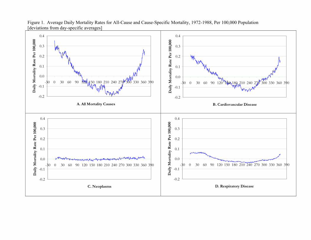
Figure 1. Average Daily Mortality Rates for All-Cause and Cause-Specific Mortality, 1972-1988, Per 100,000 Population [deviations from day-specific averages]

-0.2

-0.1

0.0

0.1

0.2

0.3

0.4

-30 0 30 60 90 120 150 180 210 240 270 300 330 360 390

A. All Mortality Causes

Dai

ly M

orta

lity

Rat

e P

er 1

00,0

00

-0.2

-0.1

0.0

0.1

0.2

0.3

0.4

-30 0 30 60 90 120 150 180 210 240 270 300 330 360 390

B. Cardiovascular Disease

Dai

ly M

orta

lity

Rat

e P

er 1

00,0

00

-0.2

-0.1

0.0

0.1

0.2

0.3

0.4

-30 0 30 60 90 120 150 180 210 240 270 300 330 360 390

C. Neoplasms

Dai

ly M

orta

lity

Rat

e P

er 1

00,0

00

-0.2

-0.1

0.0

0.1

0.2

0.3

0.4

-30 0 30 60 90 120 150 180 210 240 270 300 330 360 390

D. Respiratory Disease

Dai

ly M

orta

lity

Rat

e P

er 1

00,0

00

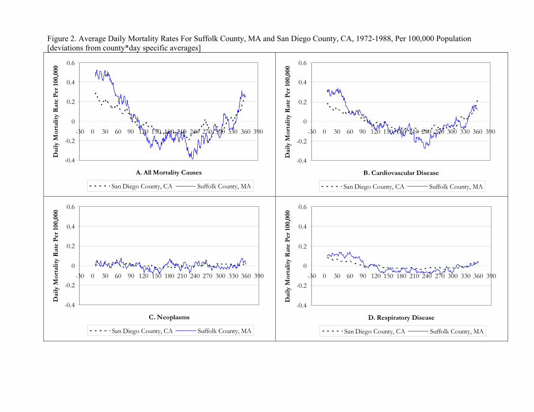
Figure 2. Average Daily Mortality Rates For Suffolk County, MA and San Diego County, CA, 1972-1988, Per 100,000 Population [deviations from county*day specific averages]

-0.4

-0.2

0

0.2

0.4

0.6

-30 0 30 60 90 120 150 180 210 240 270 300 330 360 390

A. All Mortality Causes

Dai

ly M

orta

lity

Rat

e P

er 1

00,0

00

San Diego County, CA Suffolk County, MA

-0.4

-0.2

0

0.2

0.4

0.6

-30 0 30 60 90 120 150 180 210 240 270 300 330 360 390

B. Cardiovascular Disease

Dai

ly M

orta

lity

Rat

e P

er 1

00,0

00

San Diego County, CA Suffolk County, MA

-0.4

-0.2

0

0.2

0.4

0.6

-30 0 30 60 90 120 150 180 210 240 270 300 330 360 390

C. Neoplasms

Dai

ly M

orta

lity

Rat

e P

er 1

00,0

00

San Diego County, CA Suffolk County, MA

-0.4

-0.2

0

0.2

0.4

0.6

-30 0 30 60 90 120 150 180 210 240 270 300 330 360 390

D. Respiratory Disease

Dai

ly M

orta

lity

Rat

e P

er 1

00,0

00

San Diego County, CA Suffolk County, MA

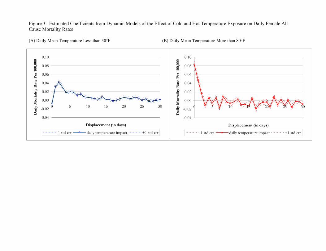
Figure 3. Estimated Coefficients from Dynamic Models of the Effect of Cold and Hot Temperature Exposure on Daily Female All-Cause Mortality Rates (A) Daily Mean Temperature Less than 30°F (B) Daily Mean Temperature More than 80°F

-0.04

-0.02

0.00

0.02

0.04

0.06

0.08

0.10

0 5 10 15 20 25 30

Displacement (in days)

Dai

ly M

orta

lity

Rat

e P

er 1

00,0

00

-1 std err daily temperature impact +1 std err

-0.04

-0.02

0.00

0.02

0.04

0.06

0.08

0.10

0 5 10 15 20 25 30

Displacement (in days)

Dai

ly M

orta

lity

Rat

e P

er 1

00,0

00

-1 std err daily temperature impact +1 std err

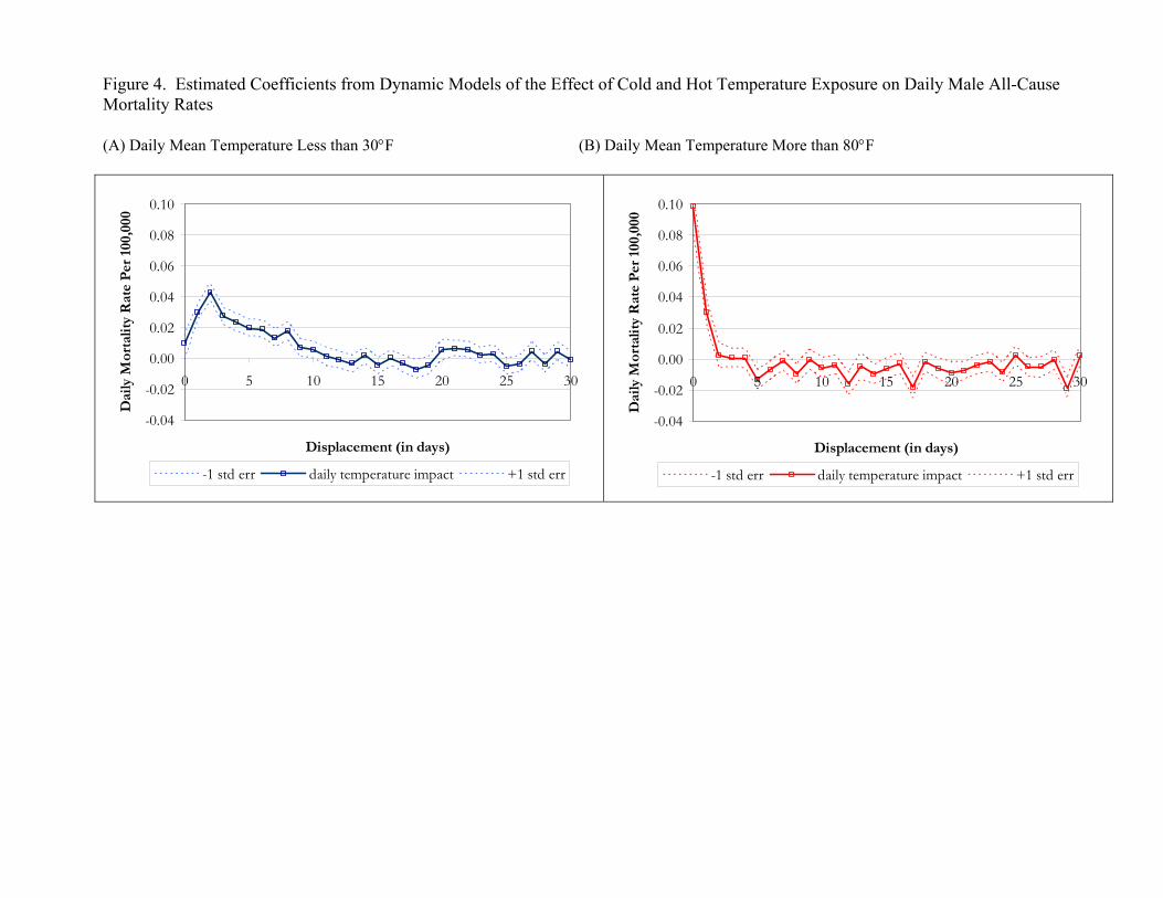
Figure 4. Estimated Coefficients from Dynamic Models of the Effect of Cold and Hot Temperature Exposure on Daily Male All-Cause Mortality Rates (A) Daily Mean Temperature Less than 30°F (B) Daily Mean Temperature More than 80°F

-0.04

-0.02

0.00

0.02

0.04

0.06

0.08

0.10

0 5 10 15 20 25 30

Displacement (in days)

Dai

ly M

orta

lity

Rat

e P

er 1

00,0

00

-1 std err daily temperature impact +1 std err

-0.04

-0.02

0.00

0.02

0.04

0.06

0.08

0.10

0 5 10 15 20 25 30

Displacement (in days)

Dai

ly M

orta

lity

Rat

e P

er 1

00,0

00

-1 std err daily temperature impact +1 std err

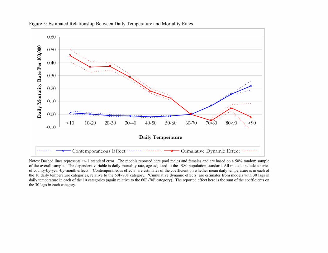
Figure 5: Estimated Relationship Between Daily Temperature and Mortality Rates

-0.10

0.00

0.10

0.20

0.30

0.40

0.50

0.60

<10 10-20 20-30 30-40 40-50 50-60 60-70 70-80 80-90 >90

Daily Temperature

Dai

ly M

orta

lity

Rat

e P

er 1

00,0

00

Contemporaneous Effect Cumulative Dynamic Effect

Notes: Dashed lines represents +/- 1 standard error. The models reported here pool males and females and are based on a 50% random sample of the overall sample. The dependent variable is daily mortality rate, age-adjusted to the 1980 population standard. All models include a series of county-by-year-by-month effects. ‘Contemporaneous effects’ are estimates of the coefficient on whether mean daily temperature is in each of the 10 daily temperature categories, relative to the 60F-70F category. ‘Cumulative dynamic effects’ are estimates from models with 30 lags in daily temperature in each of the 10 categories (again relative to the 60F-70F category). The reported effect here is the sum of the coefficients on the 30 lags in each category.

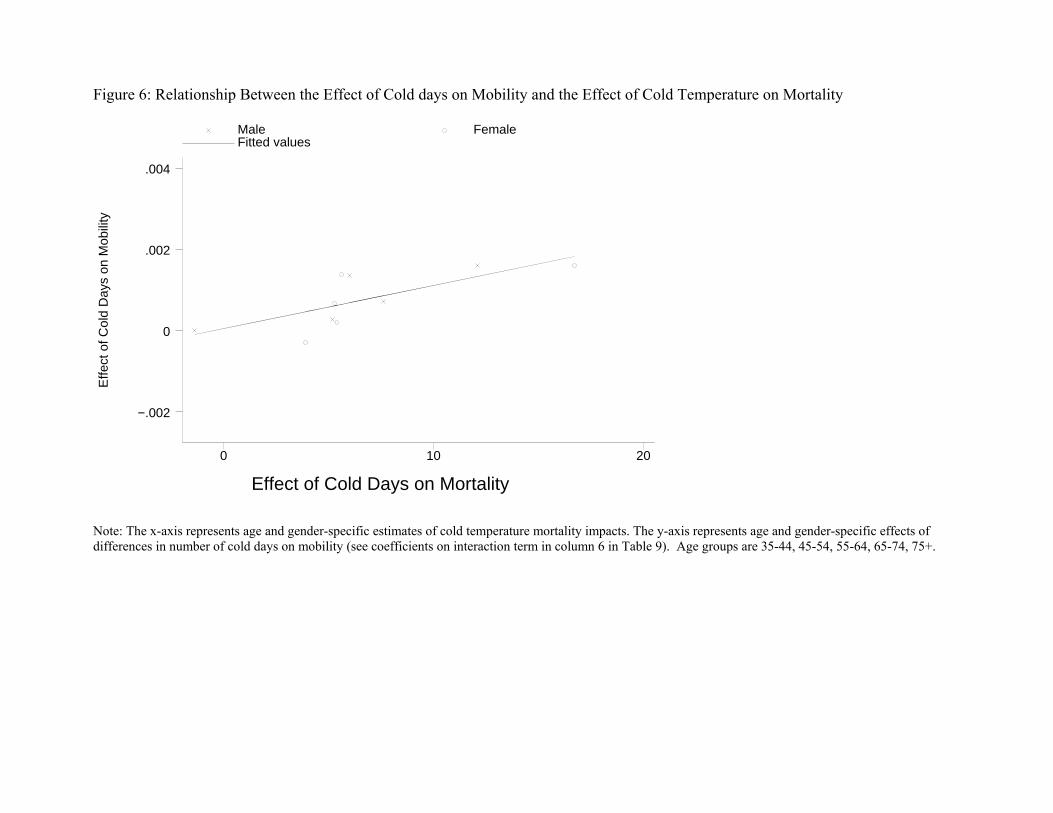
Figure 6: Relationship Between the Effect of Cold days on Mobility and the Effect of Cold Temperature on Mortality

Effe

ct o

f Col

d D

ays

on M

obili

ty

Effect of Cold Days on Mortality

Male Female Fitted values

0 10 20

−.002

0

.002

.004

Note: The x-axis represents age and gender-specific estimates of cold temperature mortality impacts. The y-axis represents age and gender-specific effects of differences in number of cold days on mobility (see coefficients on interaction term in column 6 in Table 9). Age groups are 35-44, 45-54, 55-64, 65-74, 75+.

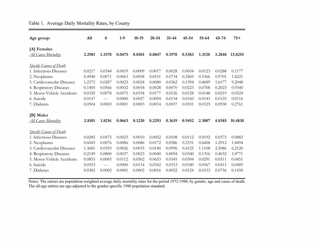
Table 1. Average Daily Mortality Rates, by County

Age group: All 0 1-9 10-19 20-34 35-44 45-54 55-64 65-74 75+

[A] FemalesAll Cause Mortality: 2.2981 1.3370 0.0475 0.0501 0.0847 0.1970 0.5383 1.3138 3.2848 13.8255

Specific Causes of Death1. Infectious Diseases 0.0217 0.0344 0.0019 0.0009 0.0017 0.0028 0.0054 0.0123 0.0288 0.11772. Neoplasms 0.4940 0.0071 0.0063 0.0058 0.0151 0.0734 0.2405 0.5366 0.9701 1.82213. Cardiovascular Diseases 1.2372 0.0287 0.0023 0.0024 0.0080 0.0362 0.1394 0.4689 1.6177 9.20484. Respiratory Diseases 0.1405 0.0566 0.0032 0.0018 0.0028 0.0070 0.0223 0.0708 0.2023 0.93405. Motor-Vehicle Accidents 0.0320 0.0078 0.0075 0.0194 0.0177 0.0126 0.0128 0.0148 0.0219 0.03246. Suicide 0.0147 --- 0.0000 0.0027 0.0094 0.0134 0.0160 0.0143 0.0125 0.01167. Diabetes 0.0504 0.0003 0.0001 0.0003 0.0014 0.0037 0.0101 0.0325 0.0930 0.2761

[B] MalesAll Cause Mortality: 2.8101 1.8216 0.0663 0.1220 0.2293 0.3619 0.9452 2.3007 4.8385 10.4830

Specific Causes of Death1. Infectious Diseases 0.0285 0.0475 0.0023 0.0010 0.0052 0.0108 0.0112 0.0192 0.0375 0.08822. Neoplasms 0.6043 0.0076 0.0086 0.0086 0.0172 0.0586 0.2331 0.6608 1.2912 1.84943. Cardiovascular Diseases 1.3681 0.0393 0.0026 0.0035 0.0140 0.0996 0.4125 1.1108 2.5086 6.21204. Respiratory Diseases 0.2149 0.0800 0.0037 0.0023 0.0040 0.0094 0.0340 0.1316 0.4032 1.07715. Motor-Vehicle Accidents 0.0853 0.0083 0.0112 0.0502 0.0653 0.0345 0.0304 0.0291 0.0311 0.04516. Suicide 0.0553 --- 0.0000 0.0114 0.0342 0.0312 0.0340 0.0367 0.0411 0.04897. Diabetes 0.0382 0.0002 0.0001 0.0002 0.0016 0.0052 0.0124 0.0333 0.0756 0.1458

Notes: The entries are population-weighted average daily mortality rates for the period 1972-1988, by gender, age and cause of death. The all-age entries are age-adjusted to the gender-specific 1980 population standard.

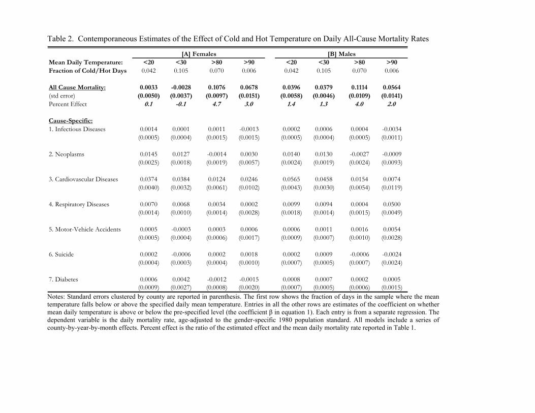
Table 2. Contemporaneous Estimates of the Effect of Cold and Hot Temperature on Daily All-Cause Mortality Rates

[A] Females [B] MalesMean Daily Temperature: <20 <30 >80 >90 <20 <30 >80 >90Fraction of Cold/Hot Days 0.042 0.105 0.070 0.006 0.042 0.105 0.070 0.006

All Cause Mortality: 0.0033 -0.0028 0.1076 0.0678 0.0396 0.0379 0.1114 0.0564(std error) (0.0050) (0.0037) (0.0097) (0.0151) (0.0058) (0.0046) (0.0109) (0.0141)Percent Effect 0.1 -0.1 4.7 3.0 1.4 1.3 4.0 2.0

Cause-Specific:1. Infectious Diseases 0.0014 0.0001 0.0011 -0.0013 0.0002 0.0006 0.0004 -0.0034

(0.0005) (0.0004) (0.0015) (0.0015) (0.0005) (0.0004) (0.0005) (0.0011)

2. Neoplasms 0.0145 0.0127 -0.0014 0.0030 0.0140 0.0130 -0.0027 -0.0009(0.0025) (0.0018) (0.0019) (0.0057) (0.0024) (0.0019) (0.0024) (0.0093)

3. Cardiovascular Diseases 0.0374 0.0384 0.0124 0.0246 0.0565 0.0458 0.0154 0.0074(0.0040) (0.0032) (0.0061) (0.0102) (0.0043) (0.0030) (0.0054) (0.0119)

4. Respiratory Diseases 0.0070 0.0068 0.0034 0.0002 0.0099 0.0094 0.0004 0.0500(0.0014) (0.0010) (0.0014) (0.0028) (0.0018) (0.0014) (0.0015) (0.0049)

5. Motor-Vehicle Accidents 0.0005 -0.0003 0.0003 0.0006 0.0006 0.0011 0.0016 0.0054(0.0005) (0.0004) (0.0006) (0.0017) (0.0009) (0.0007) (0.0010) (0.0028)

6. Suicide 0.0002 -0.0006 0.0002 0.0018 0.0002 0.0009 -0.0006 -0.0024(0.0004) (0.0003) (0.0004) (0.0010) (0.0007) (0.0005) (0.0007) (0.0024)

7. Diabetes 0.0006 0.0042 -0.0012 -0.0015 0.0008 0.0007 0.0002 0.0005(0.0009) (0.0027) (0.0008) (0.0020) (0.0007) (0.0005) (0.0006) (0.0015)

Notes: Standard errors clustered by county are reported in parenthesis. The first row shows the fraction of days in the sample where the mean temperature falls below or above the specified daily mean temperature. Entries in all the other rows are estimates of the coefficient on whether mean daily temperature is above or below the pre-specified level (the coefficient β in equation 1). Each entry is from a separate regression. The dependent variable is the daily mortality rate, age-adjusted to the gender-specific 1980 population standard. All models include a series of county-by-year-by-month effects. Percent effect is the ratio of the estimated effect and the mean daily mortality rate reported in Table 1.

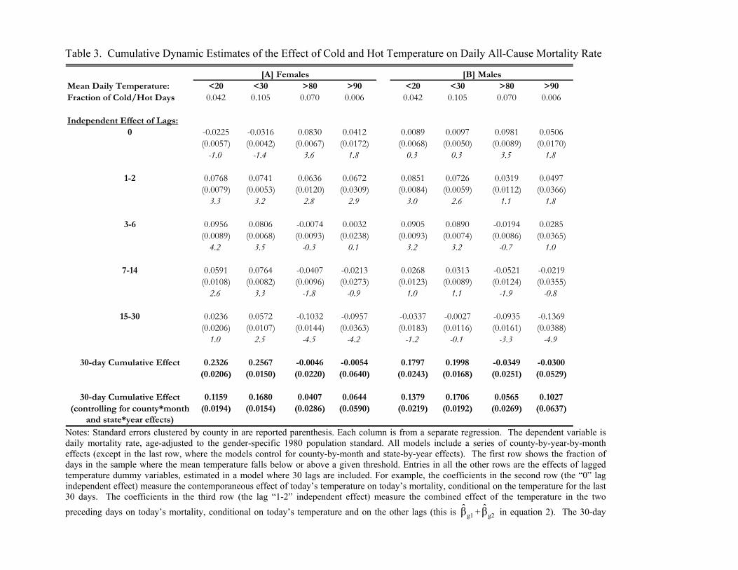
Table 3. Cumulative Dynamic Estimates of the Effect of Cold and Hot Temperature on Daily All-Cause Mortality Rate

[A] Females [B] MalesMean Daily Temperature: <20 <30 >80 >90 <20 <30 >80 >90Fraction of Cold/Hot Days 0.042 0.105 0.070 0.006 0.042 0.105 0.070 0.006

Independent Effect of Lags:0 -0.0225 -0.0316 0.0830 0.0412 0.0089 0.0097 0.0981 0.0506

(0.0057) (0.0042) (0.0067) (0.0172) (0.0068) (0.0050) (0.0089) (0.0170)-1.0 -1.4 3.6 1.8 0.3 0.3 3.5 1.8

1-2 0.0768 0.0741 0.0636 0.0672 0.0851 0.0726 0.0319 0.0497(0.0079) (0.0053) (0.0120) (0.0309) (0.0084) (0.0059) (0.0112) (0.0366)

3.3 3.2 2.8 2.9 3.0 2.6 1.1 1.8

3-6 0.0956 0.0806 -0.0074 0.0032 0.0905 0.0890 -0.0194 0.0285(0.0089) (0.0068) (0.0093) (0.0238) (0.0093) (0.0074) (0.0086) (0.0365)

4.2 3.5 -0.3 0.1 3.2 3.2 -0.7 1.0

7-14 0.0591 0.0764 -0.0407 -0.0213 0.0268 0.0313 -0.0521 -0.0219(0.0108) (0.0082) (0.0096) (0.0273) (0.0123) (0.0089) (0.0124) (0.0355)

2.6 3.3 -1.8 -0.9 1.0 1.1 -1.9 -0.8

15-30 0.0236 0.0572 -0.1032 -0.0957 -0.0337 -0.0027 -0.0935 -0.1369(0.0206) (0.0107) (0.0144) (0.0363) (0.0183) (0.0116) (0.0161) (0.0388)

1.0 2.5 -4.5 -4.2 -1.2 -0.1 -3.3 -4.9

30-day Cumulative Effect 0.2326 0.2567 -0.0046 -0.0054 0.1797 0.1998 -0.0349 -0.0300(0.0206) (0.0150) (0.0220) (0.0640) (0.0243) (0.0168) (0.0251) (0.0529)

30-day Cumulative Effect 0.1159 0.1680 0.0407 0.0644 0.1379 0.1706 0.0565 0.1027(controlling for county*month (0.0194) (0.0154) (0.0286) (0.0590) (0.0219) (0.0192) (0.0269) (0.0637)

and state*year effects) Notes: Standard errors clustered by county in are reported parenthesis. Each column is from a separate regression. The dependent variable is daily mortality rate, age-adjusted to the gender-specific 1980 population standard. All models include a series of county-by-year-by-month effects (except in the last row, where the models control for county-by-month and state-by-year effects). The first row shows the fraction of days in the sample where the mean temperature falls below or above a given threshold. Entries in all the other rows are the effects of lagged temperature dummy variables, estimated in a model where 30 lags are included. For example, the coefficients in the second row (the “0” lag independent effect) measure the contemporaneous effect of today’s temperature on today’s mortality, conditional on the temperature for the last 30 days. The coefficients in the third row (the lag “1-2” independent effect) measure the combined effect of the temperature in the two preceding days on today’s mortality, conditional on today’s temperature and on the other lags (this is g1β̂ + g2β̂ in equation 2). The 30-day

dynamic causal effect in the last row is the sum of the coefficients on the contemporaneous temperature dummy variable and the coefficients on

all lagged temperature dummy variables: ∑=

∧30

0jgjβ .

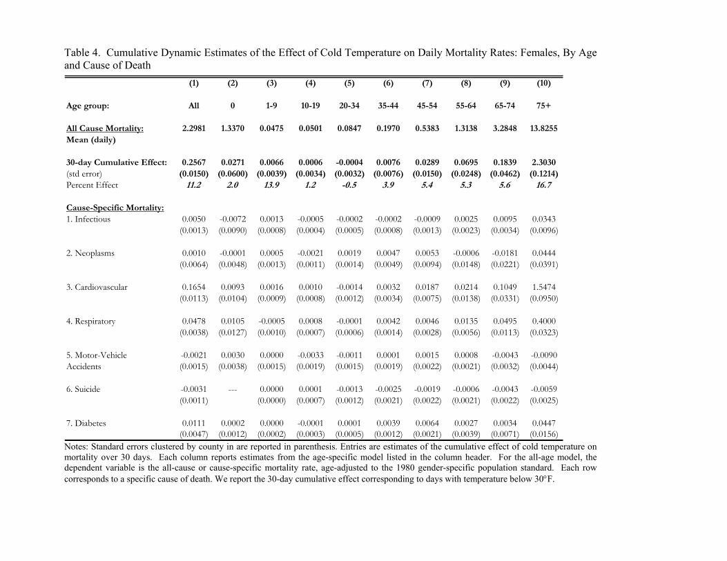
Table 4. Cumulative Dynamic Estimates of the Effect of Cold Temperature on Daily Mortality Rates: Females, By Age and Cause of Death

(1) (2) (3) (4) (5) (6) (7) (8) (9) (10)

Age group: All 0 1-9 10-19 20-34 35-44 45-54 55-64 65-74 75+

All Cause Mortality: 2.2981 1.3370 0.0475 0.0501 0.0847 0.1970 0.5383 1.3138 3.2848 13.8255Mean (daily)

30-day Cumulative Effect: 0.2567 0.0271 0.0066 0.0006 -0.0004 0.0076 0.0289 0.0695 0.1839 2.3030(std error) (0.0150) (0.0600) (0.0039) (0.0034) (0.0032) (0.0076) (0.0150) (0.0248) (0.0462) (0.1214)Percent Effect 11.2 2.0 13.9 1.2 -0.5 3.9 5.4 5.3 5.6 16.7

Cause-Specific Mortality:1. Infectious 0.0050 -0.0072 0.0013 -0.0005 -0.0002 -0.0002 -0.0009 0.0025 0.0095 0.0343

(0.0013) (0.0090) (0.0008) (0.0004) (0.0005) (0.0008) (0.0013) (0.0023) (0.0034) (0.0096)

2. Neoplasms 0.0010 -0.0001 0.0005 -0.0021 0.0019 0.0047 0.0053 -0.0006 -0.0181 0.0444(0.0064) (0.0048) (0.0013) (0.0011) (0.0014) (0.0049) (0.0094) (0.0148) (0.0221) (0.0391)

3. Cardiovascular 0.1654 0.0093 0.0016 0.0010 -0.0014 0.0032 0.0187 0.0214 0.1049 1.5474(0.0113) (0.0104) (0.0009) (0.0008) (0.0012) (0.0034) (0.0075) (0.0138) (0.0331) (0.0950)

4. Respiratory 0.0478 0.0105 -0.0005 0.0008 -0.0001 0.0042 0.0046 0.0135 0.0495 0.4000(0.0038) (0.0127) (0.0010) (0.0007) (0.0006) (0.0014) (0.0028) (0.0056) (0.0113) (0.0323)

5. Motor-Vehicle -0.0021 0.0030 0.0000 -0.0033 -0.0011 0.0001 0.0015 0.0008 -0.0043 -0.0090Accidents (0.0015) (0.0038) (0.0015) (0.0019) (0.0015) (0.0019) (0.0022) (0.0021) (0.0032) (0.0044)

6. Suicide -0.0031 --- 0.0000 0.0001 -0.0013 -0.0025 -0.0019 -0.0006 -0.0043 -0.0059(0.0011) (0.0000) (0.0007) (0.0012) (0.0021) (0.0022) (0.0021) (0.0022) (0.0025)

7. Diabetes 0.0111 0.0002 0.0000 -0.0001 0.0001 0.0039 0.0064 0.0027 0.0034 0.0447(0.0047) (0.0012) (0.0002) (0.0003) (0.0005) (0.0012) (0.0021) (0.0039) (0.0071) (0.0156)

Notes: Standard errors clustered by county in are reported in parenthesis. Entries are estimates of the cumulative effect of cold temperature on mortality over 30 days. Each column reports estimates from the age-specific model listed in the column header. For the all-age model, the dependent variable is the all-cause or cause-specific mortality rate, age-adjusted to the 1980 gender-specific population standard. Each row corresponds to a specific cause of death. We report the 30-day cumulative effect corresponding to days with temperature below 30°F.

Table 5. Cumulative Dynamic Estimates of the Effect of Cold Temperature on Daily Mortality Rates: Males, By Age and Cause of Death

(1) (2) (3) (4) (5) (6) (7) (8) (9) (10)

Age group: All 0 1-9 10-19 20-34 35-44 45-54 55-64 65-74 75+

All Cause Mortality: 2.8101 1.8216 0.0663 0.1220 0.2293 0.3619 0.9452 2.3007 4.8385 10.4830Mean (daily)

30-day Cumulative Effect: 0.1998 0.0923 0.0047 -0.0116 -0.0254 -0.0051 0.0490 0.1751 0.2915 1.2721(std error) (0.0168) (0.0753) (0.0046) (0.0047) (0.0052) (0.0108) (0.0202) (0.0304) (0.0533) (0.0983)Percent Effect 7.1 5.1 7.1 -9.5 -11.1 -1.4 5.2 7.6 6.0 12.1

Cause-Specific Mortality:1. Infectious 0.0044 0.0154 0.0001 0.0005 -0.0002 0.0008 -0.0036 0.0031 0.0083 0.0288

(0.0016) (0.0095) (0.0009) (0.0004) (0.0008) (0.0018) (0.0019) (0.0028) (0.0050) (0.0085)

2. Neoplasms -0.0003 0.0063 0.0001 0.0004 0.0001 -0.0053 0.0136 0.0322 -0.0506 0.0106(0.0075) (0.0047) (0.0005) (0.0014) (0.0015) (0.0041) (0.0099) (0.0178) (0.0269) (0.0343)

3. Cardiovascular 0.1391 0.0090 0.0005 -0.0004 -0.0014 0.0108 0.0377 0.0965 0.2107 0.7997(0.0116) (0.0096) (0.0009) (0.0009) (0.0015) (0.0058) (0.0125) (0.0221) (0.0418) (0.0707)

4. Respiratory 0.0492 0.0344 0.0023 -0.0001 0.0021 0.0012 0.0093 0.0246 0.0635 0.2846(0.0056) (0.0174) (0.0012) (0.0008) (0.0008) (0.0016) (0.0043) (0.0084) (0.0165) (0.0365)

5. Motor-Vehicle -0.0126 -0.0026 -0.0013 -0.0140 -0.0166 0.0012 -0.0023 0.0041 -0.0010 0.0054Accidents (0.0024) (0.0038) (0.0015) (0.0031) (0.0027) (0.0029) (0.0030) (0.0029) (0.0039) (0.0054)

6. Suicide -0.0072 --- 0.0001 0.0007 -0.0061 -0.0062 -0.0008 -0.0073 -0.0059 -0.0032(0.0019) (0.0001) (0.0017) (0.0022) (0.0031) (0.0034) (0.0034) (0.0038) (0.0049)

7. Diabetes 0.0049 0.0001 0.0002 0.0003 0.0003 -0.0003 0.0017 0.0025 0.0107 0.0233(0.0020) (0.0005) (0.0002) (0.0002) (0.0005) (0.0014) (0.0024) (0.0045) (0.0068) (0.0131)

Notes: Standard errors clustered by county in are reported in parenthesis. Entries are estimates of the cumulative effect of cold temperature on mortality over 30 days. Each column reports estimates from the age-specific model listed in the column header. For the all-age model, the dependent variable is the all-cause or cause-specific mortality rate, age-adjusted to the 1980 gender-specific population standard. Each row corresponds to a specific cause of death. We report the 30-day cumulative effect corresponding to days with temperature below 30°F.

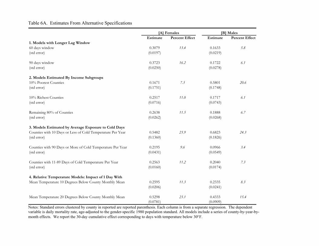
Table 6A. Estimates From Alternative Specifications

[A] Females [B] MalesEstimate Percent Effect Estimate Percent Effect

1. Models with Longer Lag Window60 days window 0.3079 13.4 0.1633 5.8(std error) (0.0197) (0.0219)

90 days window 0.3723 16.2 0.1722 6.1(std error) (0.0250) (0.0278)

2. Models Estimated By Income Subgroups10% Poorest Counties 0.1671 7.3 0.5801 20.6(std error) (0.1751) (0.1748)

10% Richest Counties 0.2517 11.0 0.1717 6.1(std error) (0.0716) (0.0743)

Remaining 80% of Counties 0.2638 11.5 0.1888 6.7(std error) (0.0262) (0.0268)

3. Models Estimated by Average Exposure to Cold DaysCounties with 10 Days or Less of Cold Temperature Per Year 0.5482 23.9 0.6823 24.3(std error) (0.1360) (0.1826)

Counties with 90 Days or More of Cold Temperature Per Year 0.2195 9.6 0.0966 3.4(std error) (0.0431) (0.0549)

Counties with 11-89 Days of Cold Temperature Per Year 0.2563 11.2 0.2040 7.3(std error) (0.0160) (0.0174)

4. Relative Temperature Models: Impact of 1 Day WithMean Temperature 10 Degrees Below County Monthly Mean 0.2595 11.3 0.2335 8.3

(0.0206) (0.0241)

Mean Temperature 20 Degrees Below County Monthly Mean 0.5298 23.1 0.4333 15.4(0.0781) (0.0909)

Notes: Standard errors clustered by county in reported are reported parenthesis. Each column is from a separate regression. The dependent variable is daily mortality rate, age-adjusted to the gender-specific 1980 population standard. All models include a series of county-by-year-by-month effects. We report the 30-day cumulative effect corresponding to days with temperature below 30°F.

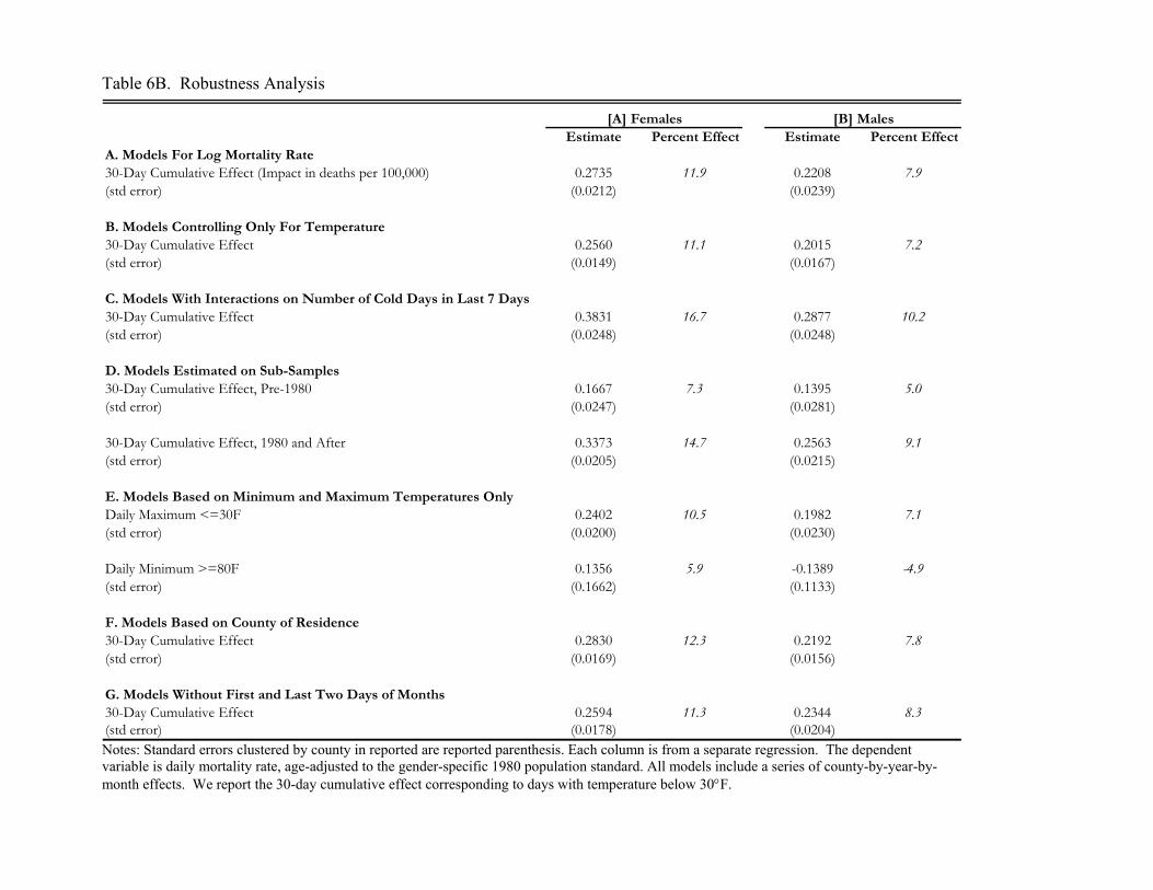
Table 6B. Robustness Analysis

[A] Females [B] MalesEstimate Percent Effect Estimate Percent Effect

A. Models For Log Mortality Rate30-Day Cumulative Effect (Impact in deaths per 100,000) 0.2735 11.9 0.2208 7.9(std error) (0.0212) (0.0239)

B. Models Controlling Only For Temperature30-Day Cumulative Effect 0.2560 11.1 0.2015 7.2(std error) (0.0149) (0.0167)

C. Models With Interactions on Number of Cold Days in Last 7 Days30-Day Cumulative Effect 0.3831 16.7 0.2877 10.2(std error) (0.0248) (0.0248)

D. Models Estimated on Sub-Samples30-Day Cumulative Effect, Pre-1980 0.1667 7.3 0.1395 5.0(std error) (0.0247) (0.0281)

30-Day Cumulative Effect, 1980 and After 0.3373 14.7 0.2563 9.1(std error) (0.0205) (0.0215)

E. Models Based on Minimum and Maximum Temperatures OnlyDaily Maximum <=30F 0.2402 10.5 0.1982 7.1(std error) (0.0200) (0.0230)

Daily Minimum >=80F 0.1356 5.9 -0.1389 -4.9(std error) (0.1662) (0.1133)

F. Models Based on County of Residence30-Day Cumulative Effect 0.2830 12.3 0.2192 7.8(std error) (0.0169) (0.0156)

G. Models Without First and Last Two Days of Months30-Day Cumulative Effect 0.2594 11.3 0.2344 8.3(std error) (0.0178) (0.0204) Notes: Standard errors clustered by county in reported are reported parenthesis. Each column is from a separate regression. The dependent variable is daily mortality rate, age-adjusted to the gender-specific 1980 population standard. All models include a series of county-by-year-by-month effects. We report the 30-day cumulative effect corresponding to days with temperature below 30°F.

Table 7. Number of Deaths caused by Cold Temperature and Years of Life Lost (1) (2) (3) (4) (5)

Age Group White Population in 2000 Cumulative Effect of 1 Cold Day Implied Annual Years of Life Lost Total YLL[in 100,000] on Mortality Per 100,000 Deaths (YLL, 2000)

[A] Females0 14.3 0.0271 15.5 80.0 1,240.11-9 133.4 0.0066 35.2 76.4 2,690.610-19 153.3 0.0006 3.7 66.5 244.720-34 226.3 -0.0004 -3.6 51.9 -187.935-44 182.5 0.0076 55.5 43.2 2,396.745-54 189.2 0.0289 218.7 32.9 7,195.755-64 107.2 0.0695 298.0 24.1 7,182.265-74 87.1 0.1839 640.7 16.2 10,379.575+ 94.5 2.3030 8,705.3 9.6 83,571.3

Annual female deaths attributable to cold temperature (all ages): 9,969 YLL per death: 11.5

[B] Males0 15.1 0.0923 55.7 74.8 4,170.01-9 140.6 0.0047 26.4 71.3 1,884.710-19 162.7 -0.0116 -75.5 61.5 -4,642.820-34 238.0 -0.0254 -241.8 47.3 -11,437.535-44 184.4 -0.0051 -37.6 38.0 -1,429.545-54 156.8 0.0490 307.3 29.0 8,912.555-64 100.6 0.1751 704.6 20.8 14,655.765-74 73.1 0.2915 852.3 13.7 11,677.175+ 55.4 1.2721 2,819.0 8.1 22,833.7

Annual male deaths attributable to cold temperature (all ages): 4,411 YLL per death: 10.6

Notes: We begin by multiplying the white population in that age group is 2000 (column 1) by the age-specific estimate of the effect of 1 cold day on mortality (column 2). The product of column 1 and 2 times 40 (the annual number of cold days for the typical county) provides an estimate of annual deaths associated with cold shocks (column 3). The product of column 3 by the years of life lost per death in each age group in column 4 represents the number of years of life lost per death caused by cold temperature (column 5). Finally, we divide column 5 by the total number of deaths attributable to cold temperature to obtain the number of years of life lost per death caused by cold temperature (YYL per death).

Table 8. Deaths caused by Cold Temperature as a Fraction of Total Deaths, by MSA Population 65+ Annual Deaths Annual Cold Days Implied Deaths % of Actual Deaths

MSA: (2000 Census) (2000 MCOD)Chicago 547,349 37,953 57 542 0.014Philadelphia 487,064 31,720 31 263 0.008New York 471,567 39,414 36 296 0.008Los Angeles 431,491 34,202 0 0 0.000Tampa Bay 374,409 21,454 0 0 0.000Detroit 355,812 23,178 69 426 0.018Boston 344,072 39,084 50 299 0.008Pittsburgh 335,190 20,914 47 271 0.013Phoenix 300,451 17,153 0 0 0.000San Jose 265,335 15,929 5 24 0.002Riverside 248,503 15,722 0 0 0.000Washington DC 246,401 15,462 28 121 0.008Minneapolis 236,316 13,997 109 448 0.032Cleveland 231,183 14,914 56 224 0.015San Diego 217,698 10,267 0 0 0.000Atlanta 215,797 13,905 9 32 0.002Baltimore 210,128 12,977 28 103 0.008West Palm Beach 203,432 13,237 0 0 0.000Houston 201,481 12,369 1 4 0.000Fort Lauderdale 180,062 11,738 0 0 0.000

Total 6,103,741 415,589 --- 3,054 0.007

Notes: In this table we focus on the population of age 65+ and on the 20 metropolitan areas with the largest number of elderly white residents.

Table 9. Estimates from Mobility Models, Mobility Defined Based on State of Birth Dependent variable is mobility indicator (=1 moved from state of birth)

Difference in annual cold days -0.0077 -0.0064 -0.0061 -0.0068 -0.0048 -0.0037(0.00002) (0.00004) (0.00003) (0.00003) (0.00003) (0.0011)

Difference in annual cold days * Age35-44 --- --- --- --- --- ---45-54 --- -0.0006 -0.0006 -0.0005 -0.0003 -0.000455-64 --- -0.0013 -0.0012 -0.0012 -0.0006 -0.000865-74 --- -0.0025 -0.0024 -0.0023 -0.0013 -0.001575+ --- -0.0029 -0.0028 -0.0026 -0.0015 -0.0018

F-statisticsInteractions = 0 --- 1,383.2 1,306.5 1,222.5 481.4 621.2Interactions all equal --- 1,122.2 1,075.2 991.6 408.6 495.1

Age Dummies No Yes Yes Yes Yes YesDemographic Controls No No Yes Yes Yes YesState Birth Effects No No No Yes No YesState Residence Effects No No No No Yes Yes

Notes: Robust standard errors are reported in parenthesis. Entries are estimates of the impact of differential exposure to cold temperature on the probability of moving, by age. The dependent variable is a dummy variable equal one if the relevant individual resides in a state different than their state of birth in 2000. The level of analysis is the individual, and the data are from the 2000 Census of Population. The sample includes white males and females, born in the 48 continental states and the District of Columbia. The independent variable in column 1 is the difference in the number of cold days between the state of residence and the state of birth. In column 2, we interact the difference in the number of cold days with indicators for each age group. For example, for individuals 35-44, a one day decline in the number of annual cold exposure is associated with an increase in the probability of mobility by .0008. For individuals above 75, a one day decline in the number of annual cold exposure is associated with an increase in the probability of mobility by 0.32 percentage points. In column 3 we control for a full set of demographic variables, including sex, educational attainment, marital status, family size, work disability, weeks worked, and total income. In column 4 we include unrestricted effects for state of birth, and in column 5 we include unrestricted effects for state of residence. The model in column 5 is close to be fully saturated.