Extreme Value Statistics and Robust Filtering for

Extreme Value Statistics and Robust Filtering forHydrological DataWBS Herbstseminar 2014

Extreme Value Statistics and Robust Filtering forHydrological Data

WBS Herbstseminar 2014Bernhard Spangl1

Peter Ruckdeschel2,3

1 BOKU – Univ. of Natural Resources and Life Sciences, Vienna,Dept. of Landscape, Spatial and Infrastructure SciencesInst. of Applied Statistics and ComputingPeter-Jordan-Straße. 82, 1190 Vienna, Austria

2 Fraunhofer ITWM, Dept. of Financial Mathematics,Fraunhofer-Platz 1, 67663 Kaiserslautern, Germany

3 TU Kaiserslautern, Dept. of Mathematics,Erwin-Schrödinger-Straße, Geb 48, 67663 Kaiserslautern, Germany

[email protected]

Wien, Nov. 06, 2014

1

mailto:[email protected]

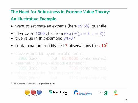
The Need for Robustness in Extreme Value Theory:

An Illustrative Example

• want to estimate an extreme (here 99.5%) quantile

• ideal data: 1000 obs. from exp(N (µ = 3, σ = 2)

)• true value in this example: 3470 ∗

• contamination: modify first 7 observations to ∼ 107

• naïve estimation by empirical quantile:2960 (ideal), but 8910000 (contaminated)

• parametric (Max-Likelihood) estimation:3390 (ideal), but 7580 (contaminated)

• robust estimation (by rmx-procedure):3440 (ideal), but 3710 (contaminated)

∗: all numbers rounded to 3 significant digits

2











2











2











2

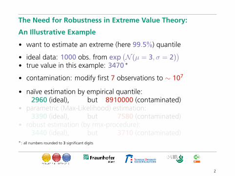
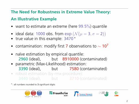
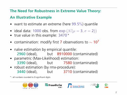
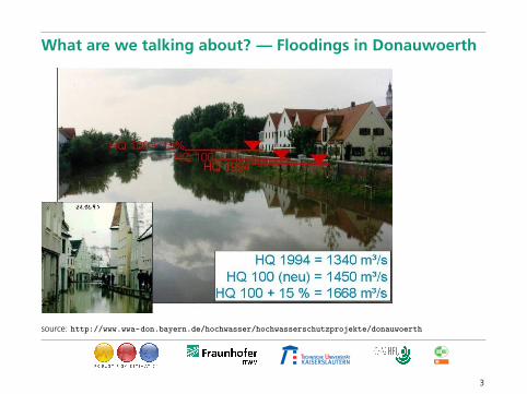
What are we talking about? — Floodings in Donauwoerth

source: http://www.wwa-don.bayern.de/hochwasser/hochwasserschutzprojekte/donauwoerth

3

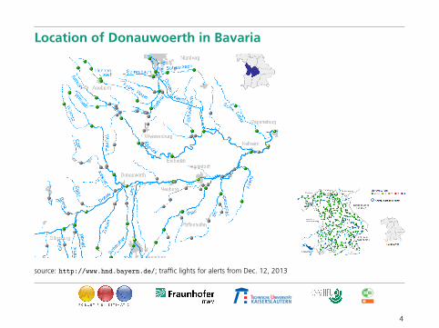
http://www.wwa-don.bayern.de/hochwasser/hochwasserschutzprojekte/donauwoerth

Location of Donauwoerth in Bavaria

source: http://www.hnd.bayern.de/; traffic lights for alerts from Dec. 12, 2013

4

http://www.hnd.bayern.de/

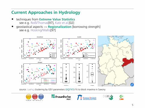
Current Approaches in Hydrology

• techniques from Extreme Value Statisticssee e.g. Reiß/Thomas[97], Katz et al.[02]

• geostastical aspects Regionalization [borrowing strength]see e.g. Hosking/Wallis[97]

●

●

● ●

●●

●

●

●

●●

●

●

●

●

●

●

●

●

●

●

●

●

●

●

●

●

●

●

●

●

●

●

●

●

●

●

●

●

●

●

●

●●●

●

●

●

●●

●

●

●

●

●

●

●

●

●

●

●

●

●

● ●

●●●

●

●

●

●

●

●

●

●

●●●

●

●

●

●

●●

4500000 4550000 4600000 4650000 4700000

5580

000

5620

000

5660

000

5700

000

location

km

km

●

●

Symbolin boxabovebelow

●

●

● ●

●●

●

●

●

●●

●

●

●

●

●

●

●

●

●

●

●

●

●

●

●

●

●

●

●

●

●

●

●

●

●

●

●

●

●

●

●

●●●

●

●

●

●●

●

●

●

●

●

●

●

●

●

●

●

●

●

● ●

●●●

●

●

●

●

●

●

●

●

●●●

●

●

●

●

●●

4500000 4550000 4600000 4650000 4700000

5580

000

5620

000

5660

000

5700

000

scale

km

km

●

●

●

Sizein boxbetw. box&whiskeroutlier

●

● ●

●●

●

●

●

●

●

●

●

●

●

●

●

●

●●

●

●

●●

●

●

●

●

●

●

●

●

●

●

●

●

●

●

●

●

●

●

●

●

●●

●

●

●

●

●

●

●

●

●

●

●

●●

●

●

●

●

●

●●

●

●

●

●

●

●

●

●

●

●●

●

●

●

●

●●

●

●

●

4500000 4550000 4600000 4650000 4700000

5580

000

5620

000

5660

000

5700

000

shape

km

km

ColorCluster 1Cluster 2Cluster 3

Cluster 4Cluster 5Cluster 6

●

●

●

●

●

●●

●

●

●

●

●

●

●

010

020

030

0

location

●

●

●

●

●

●

●

●

●

●

●

●

●

●

050

100

150

scale

●

●

●

●

0.00.5

1.0shape

source: Laaha; clustering by GEV parameters (agnes) fit to block maxima in Saxony

5

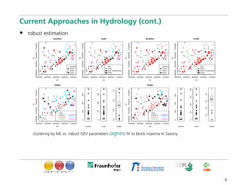
Current Approaches in Hydrology (cont.)

• robust estimation

●

●

● ●

●●

●

●

●

●●

●

●

●

●

●

●

●

●

●

●

●

●

●

●

●

●

●

●

●●

●

●

●

●

●

●

●

●●

●

●

●●●

●

●

●

●●

●

●

●

●

●

●

●

●

● ●

●

●

●

● ●

●●●

●

●

●

●

●

●

●

●

●●●

●

●

●

●

●●

4500000 4550000 4600000 4650000 4700000

5580

000

5620

000

5660

000

5700

000

location

km

km

●

●


●

●

● ●

●●

●

●

●

●●

●

●

●

●

●

●

●

●

●

●

●

●

●

●

●

●

●

●

●●

●

●

●

●

●

●

●

●

●●

●

●●●

●

●

●

●●

●

●

●

●

●

●

●

●

● ●

●

●

●

● ●

●●●

●

●

●

●

●

●

●

●

●●●

●

●

●

●

●●

4500000 4550000 4600000 4650000 4700000

5580

000

5620

000

5660

000

5700

000

scale

kmkm

●

●

●


●

● ●

●●

●

●

●

●

●

●

●

●

●

●

●

●

●●

●

●

●●

●

●

●

●

●

●

●

●

●

●

●

●

●

●

●

●

●

●●

●●

●

●

●

●

●

●

●

●●

●

●

●●

●●

●

●

●

●

●●

●

●

●

●

●

●

●

●

●

●

●● ●

●

●

●●

●

●

●

4500000 4550000 4600000 4650000 4700000

5580

000

5620

000

5660

000

5700

000

shape

km

km



●

●

●

●

●

●●

●

●

●

●

●

●

●

010

020

030

0

location

●

●

●

●

●

●●

●

●

●

●

●

●

●

●

050

100

150

scale

●

●

●

●

●●

−0.

50.

00.

51.

0

shape

●

●

● ●

●●

●

●

●

●●

●

●

●

●

●

●

●

●

●

●

●

●

●

●

●

●

●

●

●●

●

●

●

●

●

●

●

●●

●

●

●●●

●

●

●

●●

●

●

●

●

●

●

●

●

● ●

●

●

●

● ●

●●●

●

●

●

●

●

●

●

●

●●●

●

●

●

●

●●

4500000 4550000 4600000 4650000 4700000

5580

000

5620

000

5660

000

5700

000

location

km

km

●

●


●

●

● ●

●●

●

●

●

●●

●

●

●

●

●

●

●

●

●

●

●

●

●

●

●

●

●

●

●●

●

●

●

●

●

●

●

●

●●

●

●●●

●

●

●

●●

●

●

●

●

●

●

●

●

● ●

●

●

●

● ●

●●●

●

●

●

●

●

●

●

●

●●●

●

●

●

●

●●

4500000 4550000 4600000 4650000 4700000

5580

000

5620

000

5660

000

5700

000

scale

km

km

●

●

●


●

● ●

●●

●

●

●

●

●

●

●

●

●

●

●

●

●●

●

●

●

●

●

●

●●

●

●

●

●

●

●

●

●

●

●

●

●

●●

●●

●

●

●

●

●

●

●●

●

●

●

●

●

●

●●

●

●●

●

●

●

●

●

●

●

●

●

●

●●

●

●

●

●

●●

●

●

●

●●

4500000 4550000 4600000 4650000 4700000

5580

000

5620

000

5660

000

5700

000

shape

kmkm



●

●

●

●●

●●

●

●

●●

●

●

●

010

020

030

0

location

●

●

●

●

●

●

●

●

●●

●

●

●

050

100

150

200

scale

●

●

●

−1.

0−

0.5

0.0

0.5

shape

clustering by ML vs. robust GEV parameters (agnes) fit to block maxima in Saxony

6

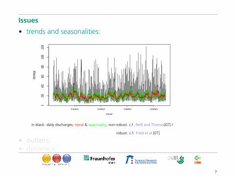
Issues

• trends and seasonalities:

1940 1960 1980 2000

020

040

060

080

010

0012

00

year

disch

arge

in black: daily discharges; trend & seasonality; non-robust: c.f. Reiß and Thomas[07] /

robust: c.f. Fried et al.[07]

• outliers:• dynamics:

7

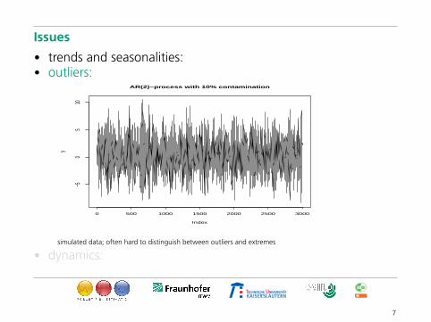
Issues

• trends and seasonalities:• outliers:

0 500 1000 1500 2000 2500 3000

−50

510

AR(2)−process with 10% contamination

Index

y

simulated data; often hard to distinguish between outliers and extremes

• dynamics:

7

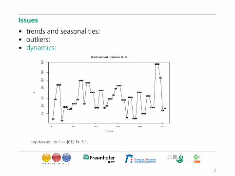
Issues

• trends and seasonalities:• outliers:• dynamics:

●

●

● ●

●

● ●

● ●

● ●

●

● ●

●

● ●

● ●

● ●

● ●

●

●

● ●

●

●

● ●

● ●

●

● ●

● ●

● ●

● ●

● ●

● ●

● ●

●

●

●

0 10 20 30 40 50

0.51.0

2.05.0

10.0

20.0

50.0

Extremal index 0.5

Index

x

toy data acc. to Coles[01], Ex. 5.1.

7

Research Questions and Challenges

• find models and robust procedures which

– capture extreme behaviour– provide a simple & parsimonious, yet flexible dynamics– possibly account for regional effects

• address the question:

inter-arrival time distribution of extremes

no new question: see, e.g., Khaliq et al.[06]

8

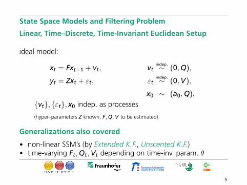
State Space Models and Filtering Problem

Linear, Time–Discrete, Time-Invariant Euclidean Setup

ideal model:

xt = Fxt−1 + vt, vtindep.∼ (0,Q),

yt = Zxt + εt, εtindep.∼ (0,V),

x0 ∼ (a0,Q),

{vt}, {εt}, x0 indep. as processes

(hyper–parameters Z known, F,Q,V to be estimated)

Generalizations also covered

• non-linear SSM’s (by Extended K.F., Unscented K.F.)• time-varying Ft,Qt,Vt depending on time-inv. param. θ

9

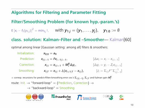
Algorithms for Filtering and Parameter Fitting

Filter/Smoothing Problem (for known hyp.-param.’s)

E∣∣xi − ft(y1:j)

∣∣2 = minft!, with y1:j = (y1, . . . , yj), y1:0 := ∅

class. solution: Kalman–Filter and –Smoother— Kalman[60]

optimal among linear [Gaussian setting: among all] filters & smoothers:

Initialization: x0|0 = a0

Prediction: xi|i−1 = Fxi−1|i−1, [∆xi = xi − xi|i−1]

Correction: xi|i = xi|i−1 + M0i ∆yi, [∆yi = yi − Zixi|i−1]

Smoothing: xi|T = xi|i + Ji(xi+1|T − xi|i), [Ji = Σi|iFτΣ−1

i|i−1]

+ corresp. recursions for predict-/filter-/smoothing error cov.’s Σi|i[−1],Σi|T and Kalman gain M0i

route: Init.→ “forward-loop” = {Prediction, Correction} →→ “backward-loop” = Smoothing

10

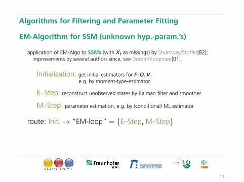
Algorithms for Filtering and Parameter Fitting

EM-Algorithm for SSM (unknown hyp.-param.’s)

application of EM-Algo to SSMs (with Xt as missings) by Shumway/Stoffer[82];improvements by several authors since, see Durbin/Koopman[01].

Initialization: get initial estimators for F,Q,V ,e.g. by moment-type-estimator

E–Step: reconstruct unobserved states by Kalman filter and smoother

M–Step: parameter estimation, e.g. by (conditional) ML estimator

route: Init.→ “EM-loop” = {E–Step, M–Step}

11

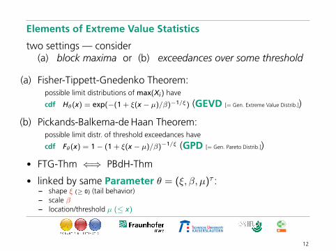
Elements of Extreme Value Statistics

two settings — consider(a) block maxima or (b) exceedances over some threshold

(a) Fisher-Tippett-Gnedenko Theorem:possible limit distributions of max(Xi) have

cdf Hθ(x) = exp(−(1 + ξ(x − µ)/β)−1/ξ) (GEVD [= Gen. Extreme Value Distrib.])

(b) Pickands-Balkema-de Haan Theorem:possible limit distr. of threshold exceedances have

cdf Fθ(x) = 1− (1 + ξ(x − µ)/β)−1/ξ (GPD [= Gen. Pareto Distrib.])

• FTG-Thm ⇐⇒ PBdH-Thm

• linked by same Parameter θ = (ξ, β, µ)τ :– shape ξ (≥ 0) (tail behavior)– scale β– location/threshold µ (≤ x)

12

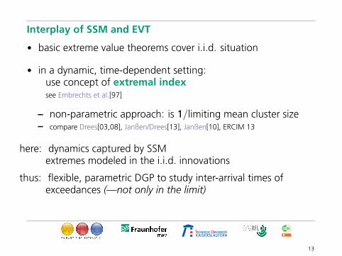
Interplay of SSM and EVT

• basic extreme value theorems cover i.i.d. situation

• in a dynamic, time-dependent setting:use concept of extremal indexsee Embrechts et al.[97]

– non-parametric approach: is 1/limiting mean cluster size– compare Drees[03,08], Janßen/Drees[13], Janßen[10], ERCIM 13

here: dynamics captured by SSMextremes modeled in the i.i.d. innovations

thus: flexible, parametric DGP to study inter-arrival times ofexceedances (—not only in the limit)

13

Outliers

• Outliers and extremes – a contradiction? Dell’Aquila/Embrechts[06]

• What makes an obs. an outlier? (—and not a regular extreme)

– occur rarely (usually, 5%–10%)

– uncontrollable, from unknown distr. (may vary obs.-wise), unpredictable– have no predictive power– usually: no error-free separation from ideal obs.

• In dynamic setting

exogenous outliers affecting only singular observations

AO :: εret ∼ (1− rAO)L(εid

t ) + rAOL(εdit )

SO :: yret ∼ (1− rSO)L(y id

t ) + rSOL(ydit )

endogenous outliers / structural changesIO :: ξre

t ∼ (1− rIO)L(ξidt ) + rIOL(ξdi

t )

but also trends, level shifts

14

Outliers








t ) + rAOL(εdit )


t ) + rSOL(ydit )



t )


14

Outliers








t ) + rAOL(εdit )


t ) + rSOL(ydit )



t )


14

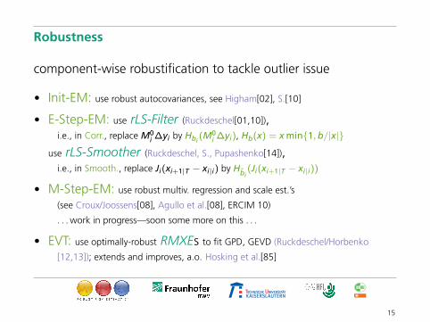
Robustness

component-wise robustification to tackle outlier issue

• Init-EM: use robust autocovariances, see Higham[02], S.[10]

• E-Step-EM: use rLS-Filter (Ruckdeschel[01,10]),i.e., in Corr., replace M0

i ∆yi by Hbi(M0

i ∆yi), Hb(x) = x min{1,b/|x|}

use rLS-Smoother (Ruckdeschel, S., Pupashenko[14]),i.e., in Smooth., replace Ji(xi+1|T − xi|i) by Hb̃i

(Ji(xi+1|T − xi|i))

• M-Step-EM: use robust multiv. regression and scale est.’s

(see Croux/Joossens[08], Agullo et al.[08], ERCIM 10)

. . . work in progress—soon some more on this . . .

• EVT: use optimally-robust RMXEs to fit GPD, GEVD (Ruckdeschel/Horbenko

[12,13]); extends and improves, a.o. Hosking et al.[85]

15

Real Data Set

• daily average discharge data of Danube river in [m3/s]

• location: gauge at Donauwörth (see initial pictures)

• start: 1923-11-01, end: 2008-12-31 (> 30,000 days)

• currently collected and provided by

Hochwassernachrichtendienst (HND),Bayerisches Landesamt für Umwelt (LfU)[translated: =̂ Flooding news service by the Bavarian Environmental Office]

• provided to us by G. Laaha within project “Robust RiskEstimation”

16

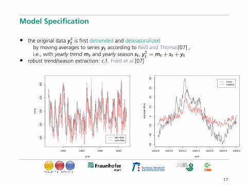
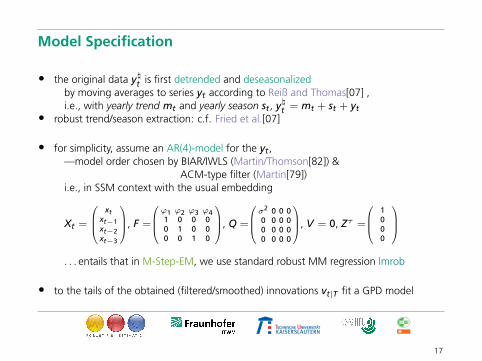
Model Specification

• the original data y\t is first detrended and deseasonalizedby moving averages to series yt according to Reiß and Thomas[07] ,i.e., with yearly trend mt and yearly season st , y\t = mt + st + yt

• robust trend/season extraction: c.f. Fried et al.[07]

1940 1960 1980 2000

100

150

200

250

300

year

trend

MA−filterwrm.filter

1923.8 1924.0 1924.2 1924.4 1924.6 1924.8 1925.0−6

0−4

0−2

00

2040

6080

year

seas

onal

effe

ct

meanmedian

17

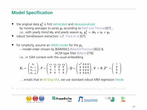
Model Specification



• for simplicity, assume an AR(4)-model for the yt ,—model order chosen by BIAR/IWLS (Martin/Thomson[82]) &

ACM-type filter (Martin[79])i.e., in SSM context with the usual embedding

Xt =

xt

xt−1xt−2xt−3

, F =

ϕ1 ϕ2 ϕ3 ϕ41 0 0 00 1 0 00 0 1 0

, Q =

σ2 0 0 00 0 0 00 0 0 00 0 0 0

, V = 0, Zτ =

1000

. . . entails that in M-Step-EM, we use standard robust MM regression lmrob

• to the tails of the obtained (filtered/smoothed) innovations vt|T fit a GPD model

17

Model Specification



• for simplicity, assume an AR(4)-model for the yt ,—model order chosen by BIAR/IWLS (Martin/Thomson[82]) &

ACM-type filter (Martin[79])i.e., in SSM context with the usual embedding

Xt =

xt

xt−1xt−2xt−3

, F =

ϕ1 ϕ2 ϕ3 ϕ41 0 0 00 1 0 00 0 1 0

, Q =

σ2 0 0 00 0 0 00 0 0 00 0 0 0

, V = 0, Zτ =

1000

. . . entails that in M-Step-EM, we use standard robust MM regression lmrob

• to the tails of the obtained (filtered/smoothed) innovations vt|T fit a GPD model

17

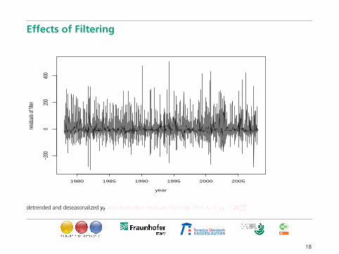
Effects of Filtering

1980 1985 1990 1995 2000 2005

−200

020

040

0

year

residu

als of

filter

detrended and deseasonalized yt and observation residuals from rob. filter ε̂t = yt − Zxrobt|t

18

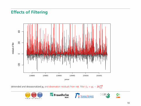
Effects of Filtering

1980 1985 1990 1995 2000 2005

−200

020

040

0

year

residu

als of

filter

detrended and deseasonalized yt and observation residuals from rob. filter ε̂t = yt − Zxrobt|t

18

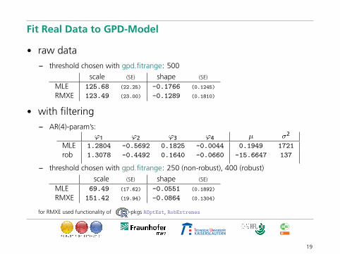
Fit Real Data to GPD-Model

• raw data– threshold chosen with gpd.fitrange: 500

scale (SE) shape (SE)

MLE 125.68 (22.25) -0.1766 (0.1245)

RMXE 123.49 (23.00) -0.1289 (0.1810)

• with filtering– AR(4)-param’s:

ϕ1 ϕ2 ϕ3 ϕ4 µ σ2

MLE 1.2804 -0.5692 0.1825 -0.0044 0.1949 1721

rob 1.3078 -0.4492 0.1640 -0.0660 -15.6647 137

– threshold chosen with gpd.fitrange: 250 (non-robust), 400 (robust)

scale (SE) shape (SE)

MLE 69.49 (17.62) -0.0551 (0.1892)

RMXE 151.42 (19.94) -0.0864 (0.1304)

for RMXE used functionality of -pkgs ROptEst, RobExtremes

19

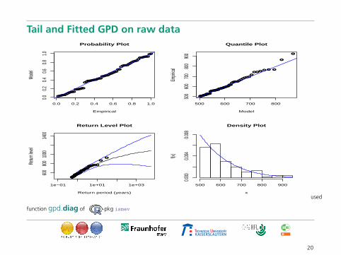
Tail and Fitted GPD on raw data

●●●●●●●●●●●●●●●●●

●●●●●●●●●●●●●●●●

●●●●●●●

●●●●●

●●●●●●

●●●●●●●

●●

0.0 0.2 0.4 0.6 0.8 1.0

0.00.2

0.40.6

0.81.0

Probability Plot

Empirical

Mode

l

●●●●●●●●●●●

●●●●●●●●●●●●

●●●●●●●●●●

●●●●●

●●●●

●●●●●

●●●●●

●● ●● ● ●

●

●

500 600 700 800

500

600

700

800

900

Quantile Plot

Model

Empir

ical

1e−01 1e+01 1e+03

600

800

1000

1400

Return Level Plot

Return period (years)

Retur

n leve

l

●●●●●●●●●●●●●●●●●●●●●●●●●●●●

●●●●●●●●●●●●●●●●●

●●●●●●

●●●●●●●

●

●

Density Plot

x

f(x)

500 600 700 800 9000.0

000.0

040.0

08

used

function gpd.diag of -pkg ismev

20

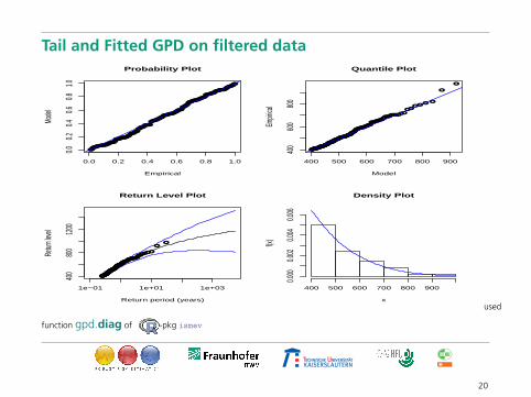
Tail and Fitted GPD on filtered data

●●●●●●

●●●●●●●●●●●●

●●●●●●●●●●●

●●●●●●●●●●

●●●●●●●●

●●●●●●●●●

●●●●●●●

●●●●●●●●●●

●●●●●●

●●●●●●●●

●●●●●●●●●●

●●●●●●●●

●●●●●●●●●●

●●●●●●

●●●●

0.0 0.2 0.4 0.6 0.8 1.0

0.00.2

0.40.6

0.81.0

Probability Plot

Empirical

Mode

l

●●●●●●●●●●●●●●●●●●●●●●

●●●●●●●●●●●●●●●●●●●

●●●●●●●●●●●●●●●●●●●

●●●●●●●●●●●●●●

●●●●●●●●●

●●●●●●●●

●●●●●●●●

●●●●●●●●

●●●●●

●●●●●●●

●●● ●

●

●

400 500 600 700 800 900

400

600

800

Quantile Plot

Model

Empir

ical

1e−01 1e+01 1e+03

400

800

1200

Return Level Plot

Return period (years)

Retur

n leve

l

●●●●●●●●●●●●●●●●●●●●●●●●●●●●●●●●●●●●●●●●●●●●●●●●●●●●●●●●●●●●●●●●●●●●●●●●●●●●●●●

●●●●●●●●●●●●●●●●

●●●●●●●●●●●●

●●●●●●●●●●

●●●●●●

●●

Density Plot

x

f(x)

400 500 600 700 800 9000.0

000.0

020.0

040.0

06

used

function gpd.diag of -pkg ismev

20

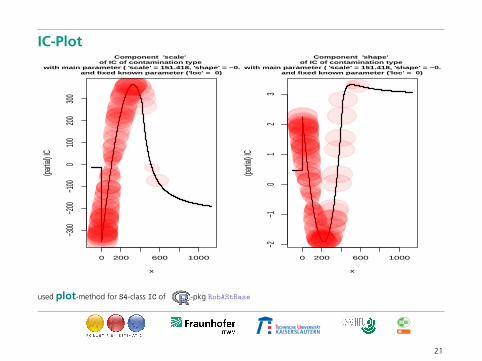
IC-Plot

0 200 600 1000

−300

−200

−100

010

020

030

0

x

(partia

l) IC

Component 'scale' of IC of contamination type

with main parameter ( 'scale' = 151.418, 'shape' = −0.086 )and fixed known parameter ('loc' = 0)

0 200 600 1000

−2−1

01

23

x

(partia

l) IC

Component 'shape' of IC of contamination type

with main parameter ( 'scale' = 151.418, 'shape' = −0.086 )and fixed known parameter ('loc' = 0)

used plot-method for S4-class IC of -pkg RobAStBase

21

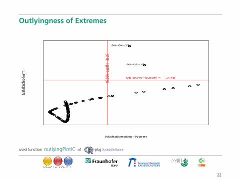
Outlyingness of Extremes

●

●

● ●

●

●●

●

●●

●

●

●

●

●

●

●

●

●●

●

●

●

●

●

●●

●

●

●

●

●

●

●

●

●

●

●

●

●

●

● ●

●

●

●

●

●

●

●●

●

●

●

●

●●

●●

●

●

●

●

●●

●

●

●

●

●

●

●

●

●

●

●

●

●

●●●

●

●

●●

●

●

●

●

●

●

●

●

●

●

●

●

●

●

●

●

●

●

●

●

●●

●

●●

●

●

●

●

●

●●

●

●

●

●●●

●

●

Mahalonobis−Norm

Maha

lonob

is−No

rm

95.00%−cutoff = 2.45

95.00

%−cu

toff =

34.2

5

90−02−15

94−04−13

used function outlyingPlotIC of -pkg RobAStBase

22

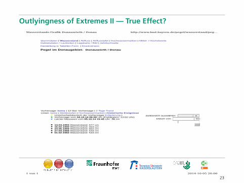
Outlyingness of Extremes II — True Effect?

Pegel im Donaugebiet: Donauwörth / Donau

Vorhersage: keine | 12-Std.-Vorhersage | 2-Tage-TrendLinien: keine | Meldestufen | Hochwassermarken | historische Ereignisse

Unsicherheitsbereich der Vorhersage( Erläuterung )Vorhersage vom 04.10.14 06:00 Uhr (Publikation: 13:02 Uhr)Letzter Messwert vom 05.10.14 19:45 Uhr: 70 cm

14.04.1994 Wasserstand: 577 cm16.02.1990 Wasserstand: 553 cm24.05.1999 Wasserstand: 552 cm27.03.1988 Wasserstand: 544 cm01.02.1982 Wasserstand: 543 cm

Zeitbereich auswählen:

Datum von: bis:

Stammdaten | Wasserstand | Abfluss | Abflusstafel | Hochwassermarken | Mittel- / HöchstwerteGebietsdaten / Laufzeiten | Lagekarte / Bild | Jahrbuchseite

Darstellung in Tabellen-Form | Druckversion

Wasserstands-Grafik Donauwörth / Donau http://www.hnd.bayern.de/pegel/wasserstand/peg...

1 von 1 2014-10-05 20:00

23

Conclusion

• presented a flexible, param. dynamic model class forhydrological extremes

• assessment of the inter-arrival distribution of extremes• provided a step-by-step robustification• evidence that robustification also enhances analysis of

extremes

24

ReferencesEmbrechts, P., Klüppelberg, C., Mikosch, T. (1997). Modelling extremal events for insurance and finance.

Springer.Fried, R., Einbeck, J., and Gather, U. (2007). Weighted Repeated Median Smoothing and Filtering, JASA 102,

1300–1308.Hosking, R.J.M., Wallis, T.J. (1997). Regional Frequency Analysis: An Approach Based on L-Moments.

Cambridge University Press.Khaliq, M.N., Ouarda, T.B.M.J., Ondo, J.-C., Gachon, P., Bobee, B. (2006). Frequency analysis of a sequence of

dependent and/or non-stationary hydro-meteorological observations: A review. Journal of Hydrology, 329,534–552.

Laaha, G., Blöschl, G. (2006). Seasonality indices for regionalizing low flows. Hydrological Processes 20(18),3851–3878.

Reiss, R.-D., Thomas, M. (2007). Statistical Analysis of Extreme Values with Applications to Insurance, Finance,Hydrology and Other Fields. Birkhäuser Verlag, Basel.

Ruckdeschel, P., Horbenko, N. (2013). Optimally-Robust Estimators in Generalized Pareto Models. Statistics47(4), 762–791.

Ruckdeschel, P., Horbenko, N. (2012). Yet another breakdown point notion: EFSBP — illustrated at scale-shapemodels. Metrika, 75 (8), 1025–1047.

Ruckdeschel, P., Spangl, B. and Pupashenko, D. (2014). Robust Kalman tracking and smoothing withpropagating and non-propagating outliers. Statistical Papers 55(1), 93–123.

Spangl, B. (2010). Computing the Nearest Correlation Matrix Which is Additionally Toeplitz. Working Paper.

THANK YOU FOR YOUR ATTENTION!

25

Documents

Extreme Value Statistics and Robust Filtering for