s 67 (2007) 189–200www.elsevier.com/locate/jmarsys

Journal of Marine System

Extreme value analysis of decadal variations instorm surge elevations

Adam Butler a,⁎, Janet E. Heffernan b, Jonathan A. Tawn b,Roger A. Flather c, Kevin J. Horsburgh c

a Biomathematics & Statistics Scotland, Kings Buildings, Edinburgh EH9 3JZ, UKb Mathematics and Statistics, Lancaster University, Lancaster LA1 4YF, UK

c Proudman Oceanographic Laboratory, 6 Brownlow Street, Liverpool L3 5DA, UK

Received 23 March 2006; received in revised form 8 September 2006; accepted 27 October 2006Available online 13 December 2006

Abstract

We use a novel statistical approach to analyse changes in the occurrence and severity of storm surge events in the southern andcentral North Sea over the period 1955–2000, using 1) output from a numerical storm surge model and 2) in situ data on surgelevels at sites for which sufficiently long observational records are available. The methodology provides a robust diagnostic tool forassessing the ability of models to reproduce the observed characteristics of storm surges, in a fashion that properly accounts bothfor variability within a single long run of the model and for recording error in observational data on sea levels.

The model re-analysis data show strong positive trends in the frequency and severity of storm surge events at locations in thenorth-eastern North Sea, whilst trends at locations in the southern and western North Sea appear to be dominated by decadalvariability. Trends in in situ data for sites along the North Sea coast are fairly synchronous with corresponding trends in the modelre-analysis data, with the most serious discrepancies attributable to known problems in the observational record.© 2006 Elsevier B.V. All rights reserved.

Keywords: Storm surges; Extreme values; Statistical modelling; Tide–surge interaction; Sea level changes; Climatic changes; European continentalshelf; North Sea

1. Introduction

Climatologists have hypothesised that climate changemay be leading to increased storminess within the NEAtlantic, and a string of empirical studies (Schinke, 1993;Schmidt and von Storch, 1993; von Storch et al., 1993;Stein and Hense, 1994; Lambert, 1996; Schmith et al.,1998; Alexandersson et al., 1998, 2000) have investigatedwhether the storm climate of the NE Atlantic has actually

⁎ Corresponding author. Tel.: +44 131 650 4896.E-mail address: adam@bioss.ac.uk (A. Butler).

0924-7963/$ - see front matter © 2006 Elsevier B.V. All rights reserved.doi:10.1016/j.jmarsys.2006.10.006

changed over the past century. The results of these studiesare somewhat inconclusive, but there is some suggestionthat the magnitude and frequency of storms may indeedhave increased over the past century, and especiallyduring the past thirty years or so.

There is virtually no empirical evidence, however, forany corresponding increase in storm surge elevations(Dixon and Tawn, 1992; Bijl et al., 1999). This absenceof evidence should not necessarily be interpreted as anevidence of absence, since (Pugh and Maul, 1999) itwould probably be difficult to detect even genuine trendswithin the relatively limited in situ data that are available.

190 A. Butler et al. / Journal of Marine Systems 67 (2007) 189–200

Trends in observational data may also be dominated byhighly localised effects, especially since tide gauges areoften based in estuarine ports which are susceptible tointensive site management (e.g. dredging).

Flather et al. (1998) show that, at least within theNorth Sea, numerical storm surge models are capable ofgenerating outputs which have similar extreme char-acteristics to those within observational data, suggestingthat surge models potentially can be used to study long-term changes in storm surge behaviour. This is theapproach which we follow in this paper.

Langenberg et al. (1999) use output from adynamical model of the North Sea to analyse trends inextreme high water levels, and find increasing trendsalong much of the European coast (but no significanttrends along the British east coast). Using a hindcast ofthe surge climate for the period 1955–2000 – which issimply an updated version of that used by Flather et al.(1998) – we investigate whether the frequency andmagnitude of storm surge events has changed over thepast fifty years. Unlike Langenberg et al. (1999), whouse winter high water levels, we concentrate solely uponthe surge process (the observed sea level minus the tidalpredictions), and use advanced statistical techniques toaccount for variability in the characteristics of simulatedstorm surge events. The methodology that we advocatehas general applicability to the detection of changes inthe magnitude and frequency of storm surge elevations,and of other quantities related to extreme sea levels.

We begin in Section 2 by briefly describing thenumerical storm surge model and observational datawhich we use. In Section 3 we introduce the statisticalmethods which we use to analyse our data: we begin bygiving an introduction to the area of extreme valuetheory, and then outline how extreme value methods canbe used to estimate temporal trends in storm surgecharacteristics. We present the results of our analysis inSection 4, and then conclude with a brief discussion.

2. Observational and model re-analysis data

2.1. Model data: the CSX–DNMI hindcast

Numerical models for surge dynamics have im-proved rapidly over recent years (Bode and Hardy,1997). The CSX model (Flather et al., 1991) wasdeveloped by the Proudman Oceanographic Laboratory(POL) as a two dimensional storm surge model for thenorth–west European continental shelf (see Fig. 1). TheCSX model is evaluated across a regular grid with aspatial resolution of 20′ in latitude and 30′ in longitude(approximately 35 km by 35 km). The model was used

as an operational model for storm surge prediction from1983 until 1991, but has since been superseded bymodels with higher spatial resolution.

Flather et al. (1998) created a hindcast of the surgeclimate for the period 1955–1992 (the “CSX–DNMIhindcast”) by forcing the CSX model using a high-quality hindcast of the meteorology for this period —the DNMI hindcast, created by Det Norske Meteor-ologiske Institut (Reistad and Iden, 1995), and used inWASA (1998). There are problems with this hindcast inareas of data sparseness, but it provides a goodrepresentation of the surge climate within the relativelydata-rich areas of the southern and central North Sea thatare of interest to us (Langenberg et al., 1999).

Atmospheric pressure and wind values from theDNMI hindcast were converted into wind stresses byinterpolating atmospheric pressure onto the CSX grid,and then applying the relationship given in Smith andBanke (1975). Tidal forcing for the CSXmodel includedeight dominant periodic constituents (Q1, O1, P1, K1,N2,M2, S2 andK2), and allowed for 18.6 year variationsin amplitude and phase. We make use of the same surgehindcast, now updated to cover the period 1955–2000.

We restrict attention to that part of the CSX gridwhich covers the southern and central North Sea. Ourmodel re-analysis data consist of 403,248 hourly surgeresiduals for each of the 259 grid cells within this region.Surge residuals are computed by deducting the levelsobtained from running the CSX model with tidal onlyforcing from those obtained by running the CSX modelwith both tidal and meteorological forcing; surgeresiduals thereby automatically incorporate the effectsof tide–surge interaction.

2.2. Observational data

We are interested, where possible, in comparingtemporal trends in surge elevations from the model re-analysis data against corresponding trends in in siturecords. Observational data are susceptible to systematicrecording errors, however, and may also be dominated byhighly localised trends (resulting, for example, fromchanging patterns of dredging). The process of removingtidal signals fromobservational sea level records in order toproduce surge records can also be highly sensitive to anyslight inaccuracies in the phase of the predicted tidal signal.It follows that asychroneities between observational andmodel re-analysis data are likely to be attributable tomodelinadequacy if they occur consistently across a number ofsites, whilst discrepancies which occur only at a single sitewill typically be attributable to problems with theobservational record at that site.

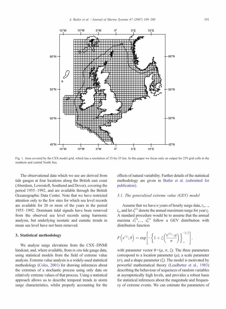
Fig. 1. Area covered by the CSX model grid, which has a resolution of 35-by-35 km. In this paper we focus only on output for 259 grid cells in thesouthern and central North Sea.

191A. Butler et al. / Journal of Marine Systems 67 (2007) 189–200

The observational data which we use are derived fromtide gauges at four locations along the British east coast(Aberdeen, Lowestoft, Southend and Dover), covering theperiod 1955–1992, and are available through the BritishOceanographic Data Centre. Note that we have restrictedattention only to the few sites for which sea level recordsare available for 20 or more of the years in the period1955–1992. Dominant tidal signals have been removedfrom the observed sea level records using harmonicanalysis, but underlying isostatic and eustatic trends inmean sea level have not been removed.

3. Statistical methodology

We analyse surge elevations from the CSX–DNMIhindcast, and, where available, from in situ tide gauge data,using statistical models from the field of extreme valueanalysis. Extreme value analysis is a widely-used statisticalmethodology (Coles, 2001) for drawing inferences aboutthe extremes of a stochastic process using only data onrelatively extreme values of that process. Using a statisticalapproach allows us to describe temporal trends in stormsurge characteristics, whilst properly accounting for the

effects of natural variability. Further details of the statisticalmethodology are given in Butler et al. (submitted forpublication).

3.1. The generalised extreme value (GEV) model

Assume that we have n years of hourly surge data, t1,…,tn, and let xj

(1) denote the annual maximum surge for year tj.A standard procedure would be to assume that the annualmaxima x1

(1),…, xn(1) follow a GEV distribution with

distribution function

F xð1Þ; h� �

¼ exp − 1þ nxð1Þ−lr

� �� �−1=n

þ

" #;

with parameter vector θ=(μ, σ, ξ). The three parameterscorrespond to a location parameter (μ), a scale parameter(σ), and a shape parameter (ξ). The model is motivated bypowerful mathematical theory (Leadbetter et al., 1983)describing the behaviour of sequences of random variablesat asymptotically high levels, and provides a robust basisfor statistical inferences about the magnitude and frequen-cy of extreme events. We can estimate the parameters of

192 A. Butler et al. / Journal of Marine Systems 67 (2007) 189–200

the model using, for example, maximum likelihood, andcan thereby obtain estimates for more easily interpretablequantities. In particular, the N-year return level

qðNÞ ¼ l−rn

1− −logN−1N

� �� �−n" #

;

corresponds to the levelwhich is exceededwith probability1/N in any particular year, and is used as a designparameter in coastal engineering applications.

3.2. The r-largest value model

The GEV model makes highly inefficient use of theavailable data, since it only allows us to use one obser-vation per year. An extension of thismodel allows us to usethe r-largest values per year, x=(x(1),…, x(r)), where r≥1is chosen a priori (see Section 3.4). The joint probabilitydensity function for the r-largest model is of the form

f ðx; hÞ ¼exp − 1þ nxðrÞ−lr

� �� �−1n

" #

jr

k¼1

1

r1þ n

xðkÞ−lr

� �� �−1n−1

;

where the parameters μ, σ and ξ correspond exactly to theparameters of the GEV model.

If we assume that the parameters of the model areconstant over time, thenmaximum likelihood estimates forthese parameters can be obtained by maximising theloglikelihood ∑j=1

n log f (xj;θ) over θ, where the vector xjcontains the r-largest values for year tj. Note that theloglikehood is a sumof contributions from each year due toan assumption of independence of extreme surges fromyear to year.

We need to ensure that the r-largest values which weselect for a particular year are drawn from distinct (andstatistically independent) storm events. We adopt thedeclustering algorithm of Tawn (1988), which sequentiallyselects the k=1,…, r largest value within a year under therestriction that the k-th largest value must lie at least s hoursaway from each of the 1st,…, (k−1)-th largest values. Thevalue of s must also be chosen a priori (see Section 3.4).

The r-largest model provides an alternative to themore usual ‘POT’ approach of fitting the generalisedpareto distribution (GPD) to peak exceedances of a highthreshold u. The POT approach cannot easily be used inthe presence of temporal and spatial variability, becausea separate threshold must be selected for each year and

site. The r-largest approach is, in contrast, robust totemporal and spatial variations, because it relies upon apurely relative definition of what constitutes an extremevalue. For example, we would need to take account oftemporal trends in mean sea level when choosing a valueof u, whereas the definition of an extreme in the r-largest model is automatically invariant to the effect ofany such trend.

3.3. Local regression models

We can model the parameters of an extreme valuemodel as a function of time (Coles, 2001; Katz et al.,2002). Let xj

(k) denote the k-th largest surge elevation inyear tj, where k≤r, and assume that xj=(xj

(1),…, xj(r) )

follows an r-largest distribution with parameter vector θj=(μj, σj, ξj).

Parametric regression models would impose aspecific structure upon the form of the temporal trendin the extreme value parameters (i.e. how θj changeswith tj), whereas nonparametric regression modelsimpose only the – relatively much weaker – assumptionthat the parameter values θj vary smoothly as functionsof time tj. The past few years have seen the rapiddevelopment of a nonparametric regression methodol-ogy within the context of extreme value modelling (Halland Tajvidi, 2000; Davison and Ramesh, 2000; Pauliand Coles, 2001; Gaetan and Grigoletto, 2004; Chavez-Demoulin and Davison, 2005), but so far there havebeen few substantive applications of these methods inthe scientific literature. In this paper we adopt thewidely-used local likelihood approach to nonparametricregression (Tibshirani and Hastie, 1987; Fan et al.,1998), using and adapting the methodology developedby Davison and Ramesh (2000) and Hall and Tajvidi(2000).

The key idea of the local likelihood approach is thatwe can estimate the parameters θj=(μj, σj, ξj) for year tjby maximising a weighted sum of loglikelihoodcontributions from all timepoints t1,…, tn. Weights aredetermined by a kernel function, K(t− tj;h), whichattributes greater weight to time points that are closeto tj than to time points which are distant from tj.

We follow Hall and Tajvidi (2000) in adopting amodel which is locally linear in the location and scaleparameters, but locally constant in the shape parameter.For year tj we numerically maximise the resulting localloglikelihood functionXnJ¼1

KðtJ−tj; hÞlog f ðxJ ; ½lj þ ajðtJ−tjÞ; rjþ bjðtJ−tjÞ; nj�Þ

193A. Butler et al. / Journal of Marine Systems 67 (2007) 189–200

over the parameter vector (μj, σj, ξj, αj, βj). The valuesof μj, σj and ξj associated with this maximum provide alocal likelihood estimator θj (h) for θj. The regressionparameters αj and βj are nuisance parameters whichquantify the rate at which the parameters μj and σj

change over time. We take the kernel function K(t− tj;h)to be a Gaussian density function with mean 0 andstandard deviation h, so that the bandwidth h determinesthe overall degree of smoothing.

3.4. Selection of r, s, and h

Our statistical model relies on our adopting suitablechoices for the number of storms per year, r, theminimum storm separation, s, and the bandwidth, h.

The asymptotic justification for the r-largest modelrelies upon r being small relative to the number ofobservations within a year. Larger values of r, however,enable us to use more data, and so lead to more efficient(i.e. less uncertain) estimates for the parameters of themodel. By plotting estimates of the model parameters as afunction of r – a ‘parameter stability plot’ (Coles, 2001) –we have a graphical tool for selecting the largest value of rbelow which the parameter estimates appear to be stable,indicating that below this value the asymptotic model isapproximately valid. We adopt a value of r=20throughout this paper, based on parameter stability plotsfor model re-analysis data at around 25 arbitrarily selectedsites in the North Sea. Note that analyses based on smallervalues of r – such as the value r=7 used by Flather et al.(1998) – yield parameter estimates which are fairlyconsistent with, but substantially more variable than,those obtained using r=20.

Trial analyses (based on the same sites as above)suggest that estimates for the extreme value parametersare largely insensitive to the value of s, so long as this istaken somewhere in the range 20–40 h. We adopts=25 h, slightly smaller than the value s=34 used byFlather et al. (1998).

The bandwidth h determines the smoothness of thelocal regression model for temporal trend – with largervalues of h corresponding to stronger levels ofsmoothing – and the choice of h is an important aspectof model choice. We adopt a bandwidth of h=3.5 yearsthroughout this paper; a kernel with this bandwidthassigns approximately 95% of weight to a 14 yearwindow around the year of interest. This choice ofbandwidth reflects both the objectives of our analysis,and our prior knowledge of the physical system: wewish to smooth out year-to-year variations in stormsurge behaviour, and to concentrate attention upon thedecadal and longer-term trends which might result from

gradual changes in levels of storminess. A range ofautomatic criteria for selecting h are available, butpreliminary results using the likelihood cross validationcriterion suggest that these will tend to select values ofthe bandwidth (h=10−20 years) which are so large thatthey will inevitably smooth out the decadal-levelvariations which we are predominantly interested indetecting. We have fitted our model using a range ofalternative bandwidths (h=2, 5 and 10 years). We findthat the detailed results of our analysis dependreasonably strongly upon the particular bandwidth thatwe have adopted, for the reasons that we have justoutlined, but that the qualitative forms of the long-termtrends in storm surge characteristics that we detect arelargely insensitive to the choice of bandwidth.

3.5. Quantifying uncertainty and assessing modelperformance

Bootstrapping is a general methodology for comput-ing the distribution of an estimator via simulation(Davison and Hinkley, 1997). We use the semi-parametric bootstrap scheme of Davison and Ramesh(2000) to quantify uncertainties in the local likelihoodestimators θ1(h),…, θn(h). The scheme involves:

(1) for each year tj transforming the data onto auniform scale via

uð1Þj ¼ F1 xð1Þj ;θjðhÞ� �

; N ; uðrÞj ¼ Fr xðrÞj ;θjðhÞ� �

;

where Fk(x(k);θ) denotes the marginal distribution

function for x(k);(2) for each j=1,…,n taking ϕj to be a random integer

between 1 and n (with replacement);(3) for each year tj transforming back onto the

original scale via

::xð1Þj ¼ F−1

1 uðrÞ/j;θjðhÞ

� �; N ;

::xðrÞj

¼ F−1r uðrÞ/j

;θjðhÞ� �

;

where F k−1 denotes the inverse of Fk ;

(4) fitting the local regression of Section 3.3 to theresampled data x1,…, xn.

This procedure is repeated B times, allowing us toobtain B independent estimates of θ1(h),…, θn(h). If thenumber of bootstrap samples B is sufficiently large then,under weak assumptions, the empirical distribution ofthese re-sampled estimates will provide a good ap-proximation to the true distribution of θ1(h),…, θn(h).

194 A. Butler et al. / Journal of Marine Systems 67 (2007) 189–200

The estimates, may, for example, be used to construct‘variability bands’ (Bowman and Azzalini, 1997). Suchbands are designed to represent uncertainty within theparameter estimates — they are similar to confidenceintervals, except that they make no attempt to adjust forthe bias involved in estimation.

Quantile–Quantile (Q–Q) plots are a widely useddiagnostic tool for comparing the distributional propertiesof a fitted statistical model against the empiricaldistribution of the data. The quantile scale acts to focusattention on the performance of the statistical model atextreme levels, so Q–Q plots are particularly appropriatefor assessing the fit of extreme value models. Theparameters of our r-largest model vary over time, so wemust standardise the fitted distributions for different yearsonto a common scale before assessing model fit. For aspecific value of kwe can construct a Q–Q plot by plotting

rðkÞj against F −1k

jnþ 1

� �;θjðhÞ

� for j ¼ 1 N ; n;

where k≤r, and where rj(k) denotes the j-th largest value in

the sequence x1(k),…, xn

(k).

4. Results and discussion

In this section we report the results from fitting ourlocal r-largest model to model re-analysis and observa-tional surge data for the period 1955–2000. Thestatistical model which we use is local linear in thelocation and scale parameters and local constant in theshape parameter, uses r=20 observations per year, andhas a bandwidth of h=3.5 years. Further details of theanalyses and results can be found in Butler (2005).

4.1. Temporal trends at specific sites

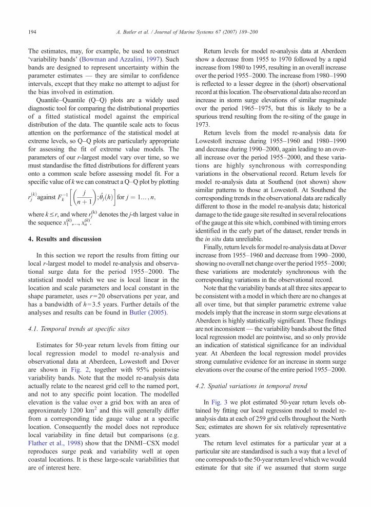
Estimates for 50-year return levels from fitting ourlocal regression model to model re-analysis andobservational data at Aberdeen, Lowestoft and Doverare shown in Fig. 2, together with 95% pointwisevariability bands. Note that the model re-analysis dataactually relate to the nearest grid cell to the named port,and not to any specific point location. The modelledelevation is the value over a grid box with an area ofapproximately 1200 km2 and this will generally differfrom a corresponding tide gauge value at a specificlocation. Consequently the model does not reproducelocal variability in fine detail but comparisons (e.g.Flather et al., 1998) show that the DNMI–CSX modelreproduces surge peak and variability well at opencoastal locations. It is these large-scale variabilities thatare of interest here.

Return levels for model re-analysis data at Aberdeenshow a decrease from 1955 to 1970 followed by a rapidincrease from 1980 to 1995, resulting in an overall increaseover the period 1955–2000. The increase from 1980–1990is reflected to a lesser degree in the (short) observationalrecord at this location. The observational data also record anincrease in storm surge elevations of similar magnitudeover the period 1965–1975, but this is likely to be aspurious trend resulting from the re-siting of the gauge in1973.

Return levels from the model re-analysis data forLowestoft increase during 1955–1960 and 1980–1990and decrease during 1990–2000, again leading to an over-all increase over the period 1955–2000, and these varia-tions are highly synchronous with correspondingvariations in the observational record. Return levels formodel re-analysis data at Southend (not shown) showsimilar patterns to those at Lowestoft. At Southend thecorresponding trends in the observational data are radicallydifferent to those in the model re-analysis data; historicaldamage to the tide gauge site resulted in several relocationsof the gauge at this site which, combinedwith timing errorsidentified in the early part of the dataset, render trends inthe in situ data unreliable.

Finally, return levels formodel re-analysis data atDoverincrease from 1955–1960 and decrease from 1990–2000,showing no overall net change over the period 1955–2000;these variations are moderately synchronous with thecorresponding variations in the observational record.

Note that the variability bands at all three sites appear tobe consistent with amodel in which there are no changes atall over time, but that simpler parametric extreme valuemodels imply that the increase in storm surge elevations atAberdeen is highly statistically significant. These findingsare not inconsistent— the variability bands about the fittedlocal regression model are pointwise, and so only providean indication of statistical significance for an individualyear. At Aberdeen the local regression model providesstrong cumulative evidence for an increase in storm surgeelevations over the course of the entire period 1955–2000.

4.2. Spatial variations in temporal trend

In Fig. 3 we plot estimated 50-year return levels ob-tained by fitting our local regression model to model re-analysis data at each of 259 grid cells throughout the NorthSea; estimates are shown for six relatively representativeyears.

The return level estimates for a particular year at aparticular site are standardised is such a way that a level ofone corresponds to the 50-year return levelwhichwewouldestimate for that site if we assumed that storm surge

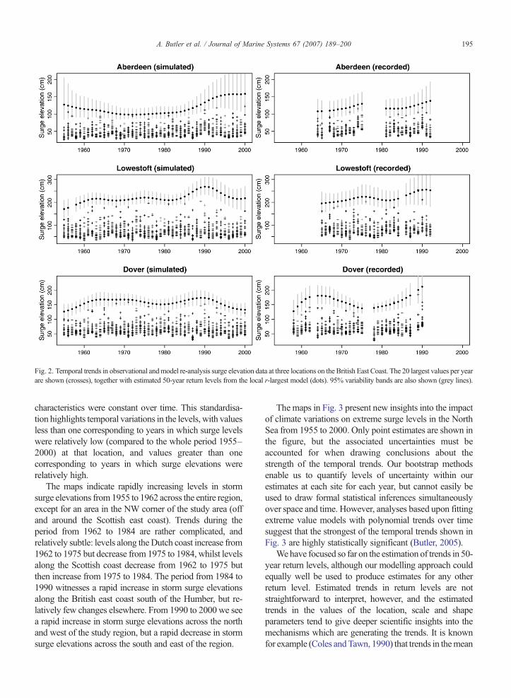
Fig. 2. Temporal trends in observational andmodel re-analysis surge elevation data at three locations on the British East Coast. The 20 largest values per yearare shown (crosses), together with estimated 50-year return levels from the local r-largest model (dots). 95% variability bands are also shown (grey lines).

195A. Butler et al. / Journal of Marine Systems 67 (2007) 189–200

characteristics were constant over time. This standardisa-tion highlights temporal variations in the levels, with valuesless than one corresponding to years in which surge levelswere relatively low (compared to the whole period 1955–2000) at that location, and values greater than onecorresponding to years in which surge elevations wererelatively high.

The maps indicate rapidly increasing levels in stormsurge elevations from1955 to 1962 across the entire region,except for an area in the NW corner of the study area (offand around the Scottish east coast). Trends during theperiod from 1962 to 1984 are rather complicated, andrelatively subtle: levels along theDutch coast increase from1962 to 1975 but decrease from 1975 to 1984, whilst levelsalong the Scottish coast decrease from 1962 to 1975 butthen increase from 1975 to 1984. The period from 1984 to1990 witnesses a rapid increase in storm surge elevationsalong the British east coast south of the Humber, but re-latively few changes elsewhere. From 1990 to 2000 we seea rapid increase in storm surge elevations across the northand west of the study region, but a rapid decrease in stormsurge elevations across the south and east of the region.

The maps in Fig. 3 present new insights into the impactof climate variations on extreme surge levels in the NorthSea from 1955 to 2000. Only point estimates are shown inthe figure, but the associated uncertainties must beaccounted for when drawing conclusions about thestrength of the temporal trends. Our bootstrap methodsenable us to quantify levels of uncertainty within ourestimates at each site for each year, but cannot easily beused to draw formal statistical inferences simultaneouslyover space and time. However, analyses based upon fittingextreme value models with polynomial trends over timesuggest that the strongest of the temporal trends shown inFig. 3 are highly statistically significant (Butler, 2005).

Wehave focused so far on the estimation of trends in 50-year return levels, although our modelling approach couldequally well be used to produce estimates for any otherreturn level. Estimated trends in return levels are notstraightforward to interpret, however, and the estimatedtrends in the values of the location, scale and shapeparameters tend to give deeper scientific insights into themechanisms which are generating the trends. It is knownfor example (Coles andTawn, 1990) that trends in themean

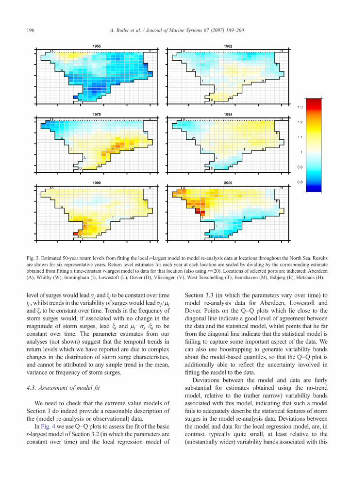
Fig. 3. Estimated 50-year return levels from fitting the local r-largest model to model re-analysis data at locations throughout the North Sea. Resultsare shown for six representative years. Return level estimates for each year at each location are scaled by dividing by the corresponding estimateobtained from fitting a time-constant r-largest model to data for that location (also using r=20). Locations of selected ports are indicated: Aberdeen(A), Whitby (W), Immingham (I), Lowestoft (L), Dover (D), Vlissingen (V), West Terschelling (T), Eemshaven (M), Esbjerg (E), Hirtshals (H).

196 A. Butler et al. / Journal of Marine Systems 67 (2007) 189–200

level of surges would leadσj and ξj to be constant over timetj , whilst trends in the variability of surges would leadσj /μjand ξj to be constant over time. Trends in the frequency ofstorm surges would, if associated with no change in themagnitude of storm surges, lead ξj and μj−σj /ξj to beconstant over time. The parameter estimates from ouranalyses (not shown) suggest that the temporal trends inreturn levels which we have reported are due to complexchanges in the distribution of storm surge characteristics,and cannot be attributed to any simple trend in the mean,variance or frequency of storm surges.

4.3. Assessment of model fit

We need to check that the extreme value models ofSection 3 do indeed provide a reasonable description ofthe (model re-analysis or observational) data.

In Fig. 4 we use Q–Q plots to assess the fit of the basicr-largest model of Section 3.2 (in which the parameters areconstant over time) and the local regression model of

Section 3.3 (in which the parameters vary over time) tomodel re-analysis data for Aberdeen, Lowestoft andDover. Points on the Q–Q plots which lie close to thediagonal line indicate a good level of agreement betweenthe data and the statistical model, whilst points that lie farfrom the diagonal line indicate that the statistical model isfailing to capture some important aspect of the data. Wecan also use boostrapping to generate variability bandsabout the model-based quantiles, so that the Q–Q plot isadditionally able to reflect the uncertainty involved infitting the model to the data.

Deviations between the model and data are fairlysubstantial for estimates obtained using the no-trendmodel, relative to the (rather narrow) variability bandsassociated with this model, indicating that such a modelfails to adequately describe the statistical features of stormsurges in the model re-analysis data. Deviations betweenthe model and data for the local regression model, are, incontrast, typically quite small, at least relative to the(substantially wider) variability bands associated with this

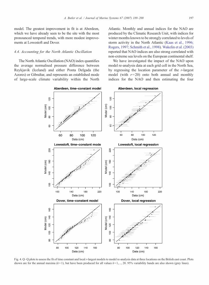
197A. Butler et al. / Journal of Marine Systems 67 (2007) 189–200

model. The greatest improvement in fit is at Aberdeen,which we have already seen to be the site with the mostpronounced temporal trends, with more modest improve-ments at Lowestoft and Dover.

4.4. Accounting for the North Atlantic Oscillation

TheNorthAtlantic Oscillation (NAO) index quantifiesthe average normalised pressure difference betweenReykjavik (Iceland) and either Ponta Delgada (theAzores) or Gibraltar, and represents an established modeof large-scale climate variability within the North

Fig. 4. Q–Q plots to assess the fit of time constant and local r-largest models toshown are for the annual maxima (k=1), but have been produced for all val

Atlantic. Monthly and annual indices for the NAO areproduced by the Climatic Research Unit, with indices forwintermonths known to be strongly correlated to levels ofstorm activity in the North Atlantic (Kaas et al., 1996;Rogers, 1997; Schmith et al., 1998). Wakelin et al. (2003)reported that NAO indices are also strong correlated withnon-extreme sea levels on the European continental shelf.

We have investigated the impact of the NAO uponmodel re-analysis data at each grid cell in the North Sea,by regressing the location parameter of the r-largestmodel (with r=20) onto both annual and monthlyindices for the NAO and then estimating the four

model re-analysis data at three locations on the British east coast. Plotsues k=1,…, 20. 95% variability bands are also shown (grey lines).

198 A. Butler et al. / Journal of Marine Systems 67 (2007) 189–200

parameters of the resulting regression models usingmaximum likelihood. We have found a strong positiverelationship between extreme surges and the annualNAO, with this relationship being statistically signifi-cant (at the 95% level) at around 90% of grid cellswithin the North Sea — mirroring the strong relation-ship at non-extreme levels reported by Wakelin et al.(2003). There are also strong positive relationships withNAO indices for each of the individual winter monthsfrom December to March. We have also investigatedwhether the long-term trends in extreme surge eleva-tions which we have estimated using our localregression model remained once we have accountedfor this effect of the NAO. We treated the estimatedregression coefficients from regressing the locationparameter of the r-largest model onto the NAO signal asa fixed “offset” term within a local regression model formodel re-analysis data at each location, and thenestimated the remaining parameters of the model usinglocal likelihood. We found that the resulting estimatesfor temporal trend did not differ qualitatively from thosewhich we obtained without accounting for the NAO.

4.5. Accounting for tide–surge interactions

The most severe coastal flood events occur whenextreme surge elevations coincide with high water ofspring tides. Tide and surge processes are dynamicallycoupled, with interactions resulting from non-linearityincluding the effects of friction and advection. In certainenvironments tide–surge interactions act to decreasesurge levels at high water whilst increasing surge levelson the rising tide (Prandle and Wolf, 1978). Suchinteractions are strongest in areas of shallow waterwhich have a large tidal range.

We have used extreme value methods to analyse the20 largest (declustered) model re-analysis surge eleva-tions to occur on a high tide— i.e. within 30 min of highwater — for each year and site. Estimates for 50-yearsurge return levels will inevitably be lower when werestrict attention only to those surges which occur inconjunction with a particular tidal state, but we find thatthe magnitude of the reduction varies markedly betweenlocations. At offshore locations in the central North Seaestimates are reduced by only 0–20 cm, but within theshallow coastal waters of the Wash, the Thames Estuaryand Heligoland Bay estimates are reduced by 100–200 cm. Despite the sometimes substantial effect oftide–surge interaction upon extreme surge elevations,we find that estimates for temporal trends in surgeelevations at high tides are qualitatively similar to thosewhich we estimate when ignoring tidal information.

5. Conclusions

We have used a novel statistical approach to studytemporal trends in the magnitude and frequency ofstorm surge elevations in the North Sea over the pastfifty years, using both observational data and model re-analysis data.

We have seen that the model re-analysis data showstrong positive trends in the north western part of ourstudy region (around the Scottish coast), and provideweak evidence for positive trends across the central andnorth-eastern part of our study region (including theGerman Bight). Surge signals in the Southern Bight, incontrast, appear to be almost entirely dominated bydecadal signals. The most pronounced temporal changesappear to occur during the periods 1955–1960(decreases in the NW, but rapid increases everywhereelse), 1980–1990 (rapid increases in the south and west,few changes elsewhere), and 1990–2000 (rapidincreases in the north and west, rapid decreases in theeast and south). Similar trends apply when we restrictattention only to surge levels associated with high tides.Extreme surge elevations are strongly related to NAOindices across most of the North Sea, but we have seenthat the decadal and longer-term trends remain once wehave accounted for the effect of NAO.

Our results differ from those of Langenberg et al.(1999), whose dynamical hindcast analysis found nosignificant trends along the British coastline but trends inwinter mean high waters along the Danish and Germancoasts; the differences may be due to our selection ofresidual as the variable of interest. The second approachof Langenberg et al. (1999) was to use regressiontechniques applied over a century of data where theyfound very small positive trends everywhere. There is nocomparable analysis in this paper, and in any case theirregression was applied to a very limited atmosphericvariable (mean sea level pressure at 5° resolution).

The trends which we have detected are clearly reliantupon the accuracy of the CSX model, and of thehindcast meteorological data which were used to forceit. The CSX–DNMI data were the best available at thetime of the analysis. Although there are more consistentre-analysis fields available now (e.g. ERA-40) they donot improve significantly on the spatial resolution here,or on the temporal resolution (6 hourly). Improvementsin computer power since the inception of this projectmean that it is now possible to repeat the analysis using asurge model with a finer spatial resolution, but theresolution of the meteorology will always be a limitingfactor in reconciling the model output with the variationof sea level seen in an observational record.

199A. Butler et al. / Journal of Marine Systems 67 (2007) 189–200

The key focus of the current paper, however, hasbeen to demonstrate a novel statistical approach for theanalysis of long-term variability in extreme sea levels,and to show how this technique can be used as a diag-nostic tool for the magnitude and frequency of stormsurges generated by sophisticated numerical models.The approach has general applicability for detecting andexploring temporal and spatial trends in the magnitudeand frequency of extreme events, and could easily beextended to deal with more complicated problems and/or to incorporate more physical information into thestatistical analysis. In particular, it is known that we canreduce the uncertainties in parameter estimates fromextreme value models by explicitly incorporatingknowledge of spatial dependence (Dixon and Tawn,1992; Dixon et al., 1998), and preliminary investiga-tions using the datasets from this paper suggesting thatthese benefits can be substantial within an oceano-graphic context (Butler et al., submitted for publication).The key practical issues with the methodology revolvearound the choice of r and the choice of h, and it isimportant to recognise that these quantities need to becarefully selected on the basis of both (a) the empiricalproperties of the dataset at hand, and (b) the scientificobjectives of the analysis. Overall, the methodologywhich we have presented provides a flexible andstatistically rigorous approach for quantifying changesin the extremal properties of oceanographic processes.

Acknowledgements

The first author was jointly funded by the Engineer-ing and Physical Sciences Research Council and theBeauclerk Memorial Fund, and undertook this workwhilst studying for a doctorate at Lancaster University.Barry Rowlingson and David Blackman providedtechnical assistance in processing the output from theCSX model. Tide gauge data for the United Kingdomwere provided by the British Oceanographic DataCentre, and NAO indices by the Climatic Research Unit.

Appendix A. Supplementary data

Supplementary data associated with this articlecan be found, in the online version, at doi:10.1016/j.jmarsys.2006.10.006.

References

Alexandersson, H., Schmith, T., Iden, K., Tuomenvirta, H., 1998.Long-term trend variations of the storm climate over NW Europe.The Global Atmosphere and Ocean System 6, 97–120.

Alexandersson, H., Tuomenvirta, H., Schmith, T., Iden, K., 2000.Trends of storms in NW Europe derived from an updated pressuredata set. Climate Research 14, 71–73.

Bijl, W., Flather, R.A., de Ronde, J.G., Schmith, T., 1999. Changingstorminess? An analysis of long-term sea level data sets. ClimateResearch 11, 161–172.

Bode, L., Hardy, T.A., 1997. Progress and recent developments in stormsurge modelling. Journal of Hydraulic Engineering 123, 315–331.

Bowman, A.W., Azzalini, A., 1997. Applied Smoothing Techniquesfor Data Analysis. Oxford University Press, Oxford.

Butler, A., 2005. Statistical Modelling of Synthetic OceanographicExtremes. Ph.D. Thesis, Lancaster University, UK, unpublished.

Butler, A., Heffernan, J.E., Tawn, J.A., Flather, R.A., submitted forpublication. Trend estimation in extremes of synthetic North Seasurges. Applied Statistics.

Chavez-Demoulin, V., Davison, A.C., 2005. Generalized additivemodelling of sample extremes. Applied Statistics 54, 207–222.

Coles, S.G., 2001. An Introduction to Statistical Modelling of ExtremeValues. Springer, London.

Coles, S.G., Tawn, J.A., 1990. Statistics of coastal flood prevention.Philosophical Transactions of the Royal Society of London. SeriesA 332, 457–476.

Davison, A.C., Hinkley, D.V., 1997. Bootstrap Methods and TheirApplication. Cambridge University Press, Cambridge.

Davison, A.C., Ramesh, N.I., 2000. Smoothing sample extremes.Journal of the Royal Statistical Society. Series B 92, 191–208.

Dixon, M.J., Tawn, J.A., 1992. Trends in UK extreme sea levels: aspatial approach. Geophysical Journal International 111, 607–616.

Dixon, M.J., Tawn, J.A., Vassie, J.M., 1998. Spatial modelling ofextreme sea-levels. Environmetrics 9, 283–301.

Fan, J.Q., Farmen, M., Gijbels, I., 1998. Local maximum likelihoodestimation and inference. Journal of the Royal Statistical Society.Series B 60, 591–608.

Flather, R.A., Proctor, R., Wolf, J., 1991. Oceanographic forecast models.In: Farmer, D.G., Rycroft, M.J. (Eds.), Computer Modelling in theEnvironmental Sciences. Clarendon Press, Oxford.

Flather, R.A., Smith, J.A., Richards, J.C., Bell, C., Blackman, D.L.,1998. Direct estimates of extreme storm surge elevations from a40-year numerical model simulation and from observations. TheGlobal Atmosphere and Ocean System 6, 165–176.

Gaetan, C., Grigoletto, M., 2004. Smoothing sample extremes withdynamic models. Extremes 7, 221–236.

Hall, P., Tajvidi, N., 2000. Nonparametric analysis of temporal trendwhen fitting parametric models to extreme-value data. StatisticalScience 15, 153–167.

Kaas, E., Li, T.-S., Schmith, T., 1996. Statistical hindcast of windclimatology in the North Atlantic and northwestern Europeanregion. Climate Research 7, 97–110.

Katz, R.W., Parlange, M.B., Naveau, P., 2002. Statistics of extremes inhydrology. Advances in Water Resources 25, 1287–1304.

Lambert, S.J., 1996. Intense extratropical Northern Hemisphere wintercyclone events: 1899–1991. Journal of Geophysical Research D.Atmospheres 101, 21319–21325.

Langenberg, H., Pfizenmayer, A., von Storch, H., Sundermann, J.,1999. Storm-related sea level variations along the North Sea coast:natural variability and anthropogenic change. Continental ShelfResearch 19, 821–842.

Leadbetter, M.R., Lindgren, G., Rootzén, H., 1983. Extremes andRelated Properties of Random Sequences and Series. Springer-Verlag, New York.

Pauli, F., Coles, S.G., 2001. Penalized likelihood inference in extremevalue analyses. Journal of Applied Statistics 28, 547–560.

200 A. Butler et al. / Journal of Marine Systems 67 (2007) 189–200

Prandle, D., Wolf, J., 1978. The interaction of surge and tide in theNorth Sea and River Thames. Geophysical Journal of the RoyalAstronomical Society 55, 203–216.

Pugh, D.T., Maul, G.A., 1999. Coastal sea level prediction for climatechange. In: Mooers, C.N.K. (Ed.), Coastal Ocean Prediction,American Geophysical Union (Coastal Studies Series), pp. 377–404.Ch.15.

Reistad, M., Iden, K.A., 1995. Updating, correction and evaluation of ahindcast data base of air pressure, winds and waves for the NorthSea, Norweigan Sea and the Barents Sea. Technical report 9, DetNorske Meteorologiske Institut, Oslo, Norway, unpublished.

Rogers, J.C., 1997. North Atlantic storm track variability and itsassociation to the North Atlantic Oscillation and climate variabilityof Northern Europe. Journal of Climate 10, 1635–1647.

Schinke, H., 1993. On the occurence of deep cyclones over Europe andthe North Atlantic in the period 1930–1991. Beiträge zur Physikder Atmosphäre 66, 223–237.

Schmidt, H., von Storch, H., 1993. German Bight storms analysed.Nature 365, 790.

Schmith, T., Kaas, E., Li, T.-S., 1998. Northeast Atlantic storminess1875–1995 re-analysed. Climate Dynamics 14, 529–536.

Smith, S.D., Banke, E., 1975. Variation of the sea surface dragcoefficient with wind speed. Quarterly Journal of the RoyalMeteorological Society 101, 665–673.

Stein, O., Hense, A., 1994. A reconstructed time series of the numberof extreme low pressure events since 1880. MeteorologischeZeitschrift NF3, 43–46.

Tawn, J.A., 1988. An extreme value theory model for dependentobservations. Journal of Hydrology 101, 227–250.

Tibshirani, R.J., Hastie, T.J., 1987. Local likelihood estimation.Journal of the American Statistical Association 82, 559–567.

von Storch, H., Guddal, J., Iden, K., Jonsson, T., Perlwitz, J., Reistad,M., de Ronde, J., Schmidt, H., Zorita, E., 1993. Changing statisticsof storms in the North Atlantic. Technical report 116, Max–PlanckInstitute for Meteorology, Hamburg, Germany, unpublished.

Wakelin, S.L., Woodworth, P.L., Flather, R.A., Williams, J.A., 2003.Sea-level dependence on the NAO over the NW EuropeanContinental Shelf. Geophysical Research Letters 30, 1403–1406.

WASA project team, 1998. Changing waves and storms in theNortheast Atlantic. Bulletin of the American MeteorologicalSociety 79, 741–760.