Extreme Value Analysis

FISH 558 Decision Analysis in Natural Resource Management

12/4/2013Noble Hendrix

QEDA Consulting LLCAffiliate Faculty UW SAFS

2

Lecture Overview

• Motivating examples of extreme events• Generalized Extreme Value– Statistical Development– Case Study: the white cliffs of Dover

• Generalized Pareto Distribution– Statistical Development– Case Study: whale strikes in SE Alaska

• Additional resources

3

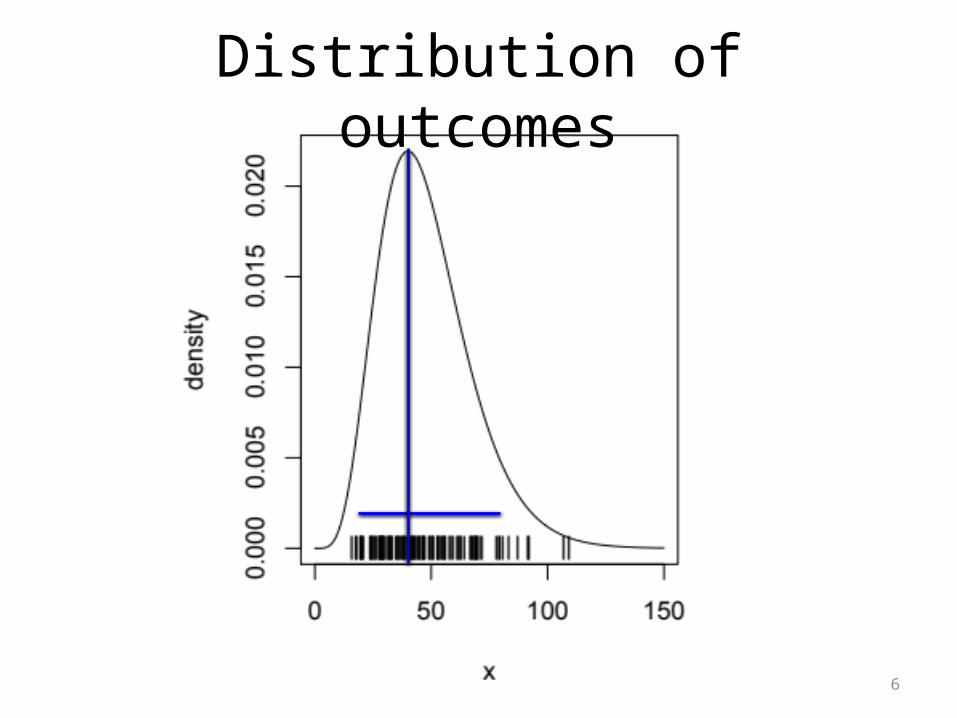
Why should we care about extreme events?

• They are rare by definition, so why spend much time thinking about them?

• Often the consequences of the event have significant impacts to the system – mortality, colonization, episodic recruitment

• We tend to focus on averages, but extremes may be more important in some situations.

• We may also be interested in estimating extremes beyond what has been observed

4

Distribution of outcomes

5

Distribution of outcomes

6

Distribution of outcomes

7

Distribution of outcomes

8

Distribution of outcomes

9

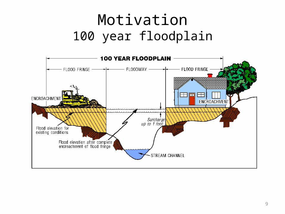
Motivation100 year floodplain

10

Motivation Surpassing the 100 year floodplain

• Road and home construction based on flood frequency and intensity i.e., 100 year floodplain

11

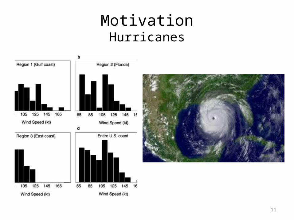
MotivationHurricanes

12

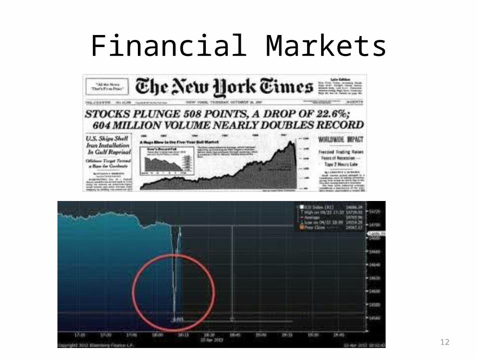
Financial Markets

Statistical Foundations 13

Central Limit Theorem

Consider sequence of iid random variables, X1, … Xn

We know that sum Sn = X1 + … + Xn, when normalized lead to the CLT:

14

Generalized Extreme ValueFisher-Tippet Asymptotic Theorem

Define maxima of sequence of random variables Mn = max(X1, …, Xn)

For normalized maxima, there is also a non-degenerate distribution H(x), which is a GEV distribution

15

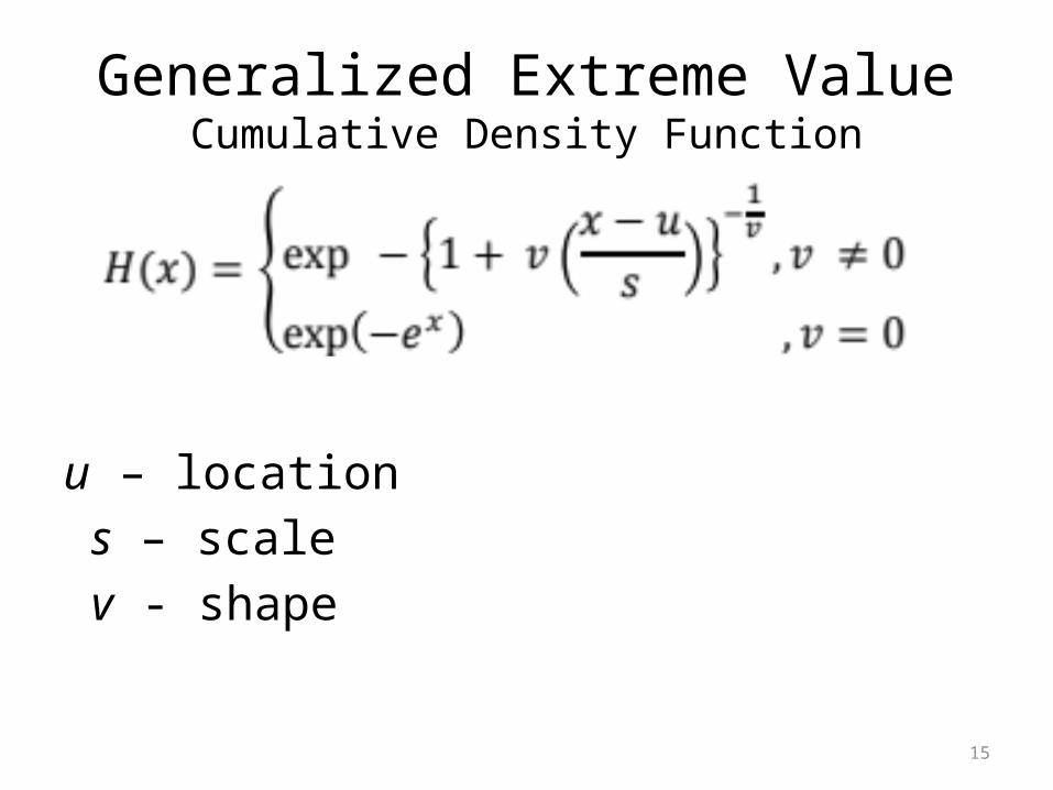
Generalized Extreme ValueCumulative Density Function

u – location s – scale v - shape

16

Generalized Extreme ValueVariants of the GEV

Shape parameter v defines several distributions:

Gumbel: v = 0

Weibull: v < 0

Fréchet: v > 0

17

Generalized Extreme ValueShapes of GEV

Weibull

Gumbel

Fréchet

18

Generalized Extreme ValueApplicability

Almost all common continuous distributions converge on H(x) for some value of v

• Weibull – beta • Gumbel – normal, lognormal, hyperbolic,

gamma, chi-squared• Fréchet – Pareto, inverse gamma, Student t,

loggamma

19

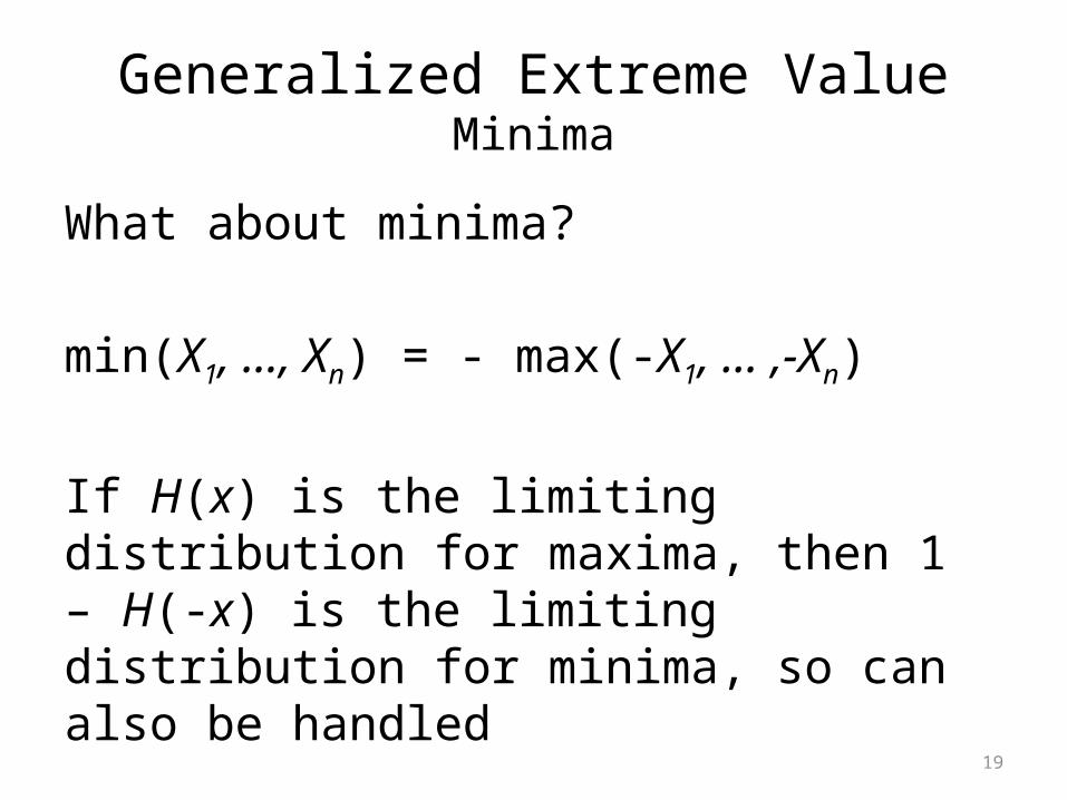
Generalized Extreme ValueMinima

What about minima?

min(X1, …, Xn) = - max(-X1, … ,-Xn)

If H(x) is the limiting distribution for maxima, then 1 – H(-x) is the limiting distribution for minima, so can also be handled

20

Generalized Extreme ValueEstimation

Obtain data from an unknown distribution F

• Let’s assume that there is an extreme value distribution Hv for some value of v

• The true distribution of the n-block maximum Mn can be approximated for large enough n with a GEV distribution H(x)

• Fit model to repeated observations of an n-block maximum, thus m blocks of size n

21

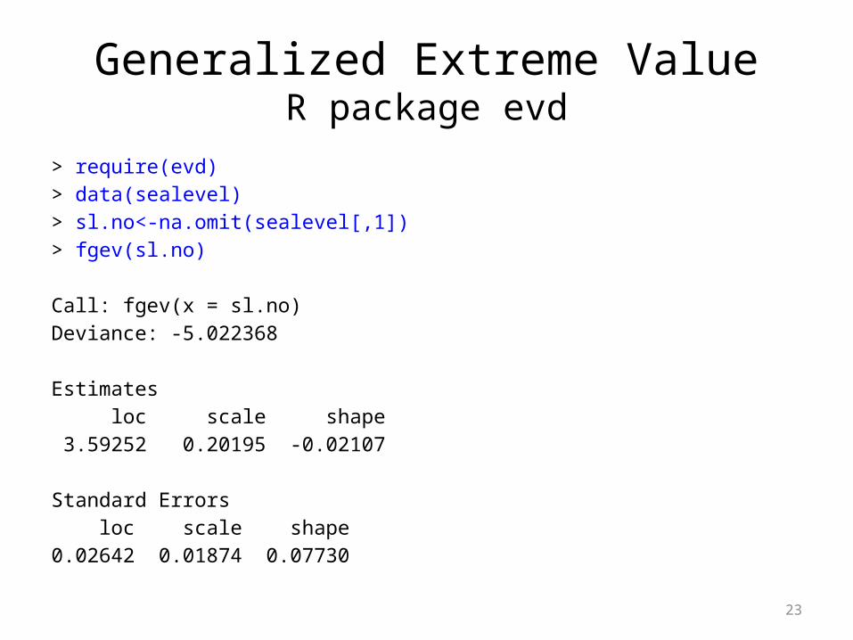
Generalized Extreme ValueExample - Data

Annual sea level height at Dover, Britain between 1912 and 1992

22

Generalized Extreme ValueExample - Data

Annual sea level height at Dover, Britain between 1912 and 1992

23

Generalized Extreme ValueR package evd

> require(evd)> data(sealevel)> sl.no<-na.omit(sealevel[,1])> fgev(sl.no)

Call: fgev(x = sl.no) Deviance: -5.022368

Estimates loc scale shape 3.59252 0.20195 -0.02107

Standard Errors loc scale shape 0.02642 0.01874 0.07730

24

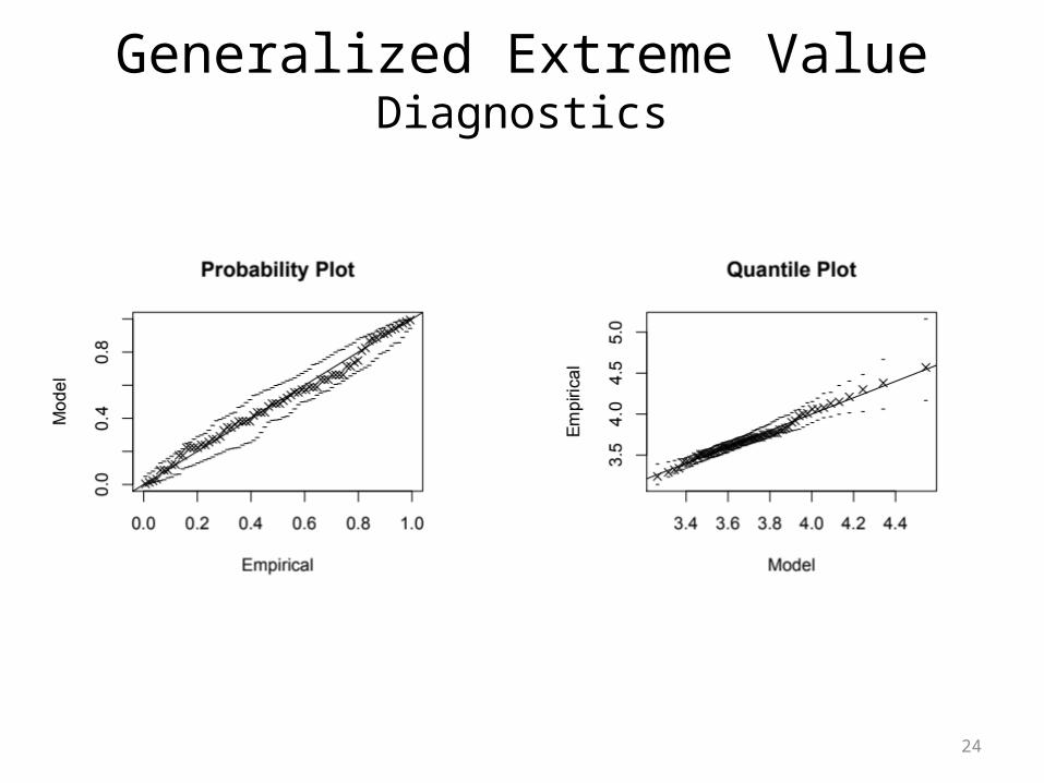
Generalized Extreme ValueDiagnostics

25

Generalized Extreme ValueReturn Level Plot

Return level – “how long to wait on average until see another event equal to or more extreme”

If H is the distribution of the n-block maximum, the k return level is the 1 – 1/k quantile of H

26

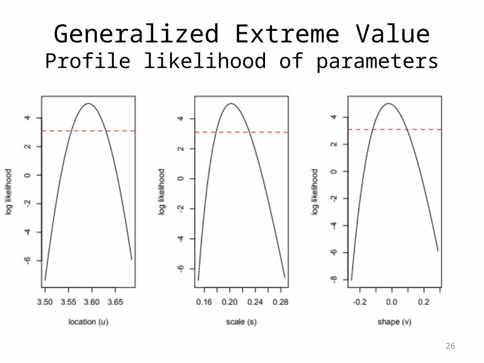
Generalized Extreme ValueProfile likelihood of parameters

27

Generalized Extreme ValueLimitations

• Limitations of the GEV:– Used for block maxima, e.g., annual

precipitation, annual flow, – Only 1 exceedance per block– May ignore some important observations,– Some go so far as to say it is a wasteful method!

(McNeil et al. 2005 Quantitative Risk Management, Princeton)

28

Generalized Pareto Distribution

GEV has largely been surpassed by another method for extremes over a threshold

Pickands (1975) developed a model for excesses y over threshold a

Pickands 1975 Annals of Stats 3:119

29

Generalized Pareto Distribution

a – thresholdb – scalev - shape

30

Generalized Pareto DistributionShapes of GPD

Positive shape =limitless loss

31

Generalized Pareto DistributionApplicability

For any continuous distributions that converge on H(x) for some value of v, which was most of the continuous distributions of interest

The same distributions will converge on G(x) as an excess distribution as the threshold a is raised

32

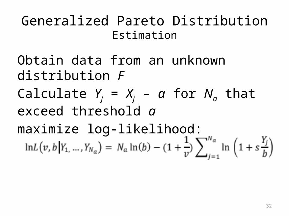
Generalized Pareto DistributionEstimation

Obtain data from an unknown distribution FCalculate Yj = Xj – a for Na that exceed threshold amaximize log-likelihood:

33

Generalized Pareto DistributionThreshold Estimation

Have an interesting problem:• Need a value of threshold a that must be

high enough to satisfy the theoretical assumptions

• Need enough data above the threshold a so that the parameters are well estimated

• Use a sample mean residual life plot to help identify a reasonable threshold value a

34

Generalized Pareto DistributionSample Mean Residual Life Plot

Let Y = X – a0. At threshold a0, if Y is GPD with parameters b and v then

E(Y) = b/(1 – v), v < 1

This is true for all thresholds ai > a0, but the scale parameter bi must be appropriate to the threshold ai

E(X-ai| X > ai) = (bi + v*ai)/(1-v),

Thus E(X - a| X > a) is a linear function of a where GPD appropriate, so can plot E(x-ai) (where x are our observed data) versus ai.

This is the sample mean residual life plot, and confidence intervals added by assuming E(x-a) are approximately normally distributed

35

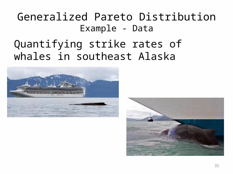
Generalized Pareto DistributionExample - Data

Quantifying strike rates of whales in southeast Alaska

36

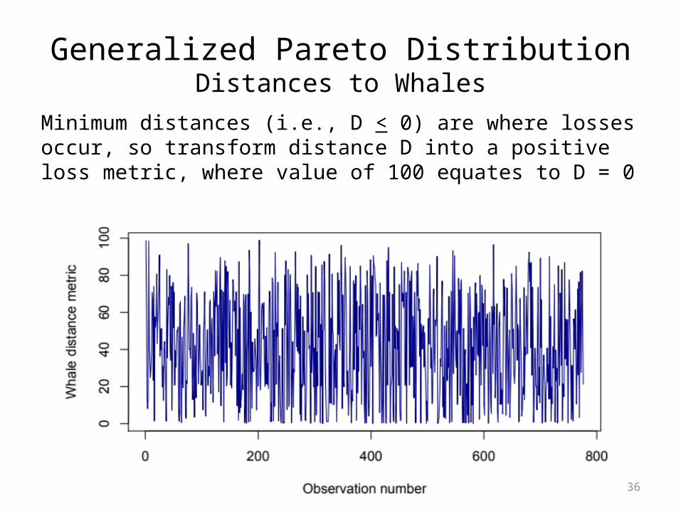
Generalized Pareto DistributionDistances to Whales

Minimum distances (i.e., D < 0) are where losses occur, so transform distance D into a positive loss metric, where value of 100 equates to D = 0

37

Generalized Pareto DistributionWhale Distance Metric

38

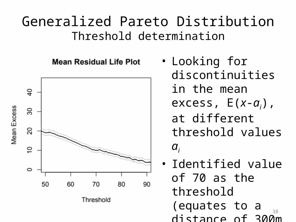
Generalized Pareto DistributionThreshold determination

• Looking for discontinuities in the mean excess, E(x-ai), at different threshold values ai

• Identified value of 70 as the threshold (equates to a distance of 300m between whales and ships)

39

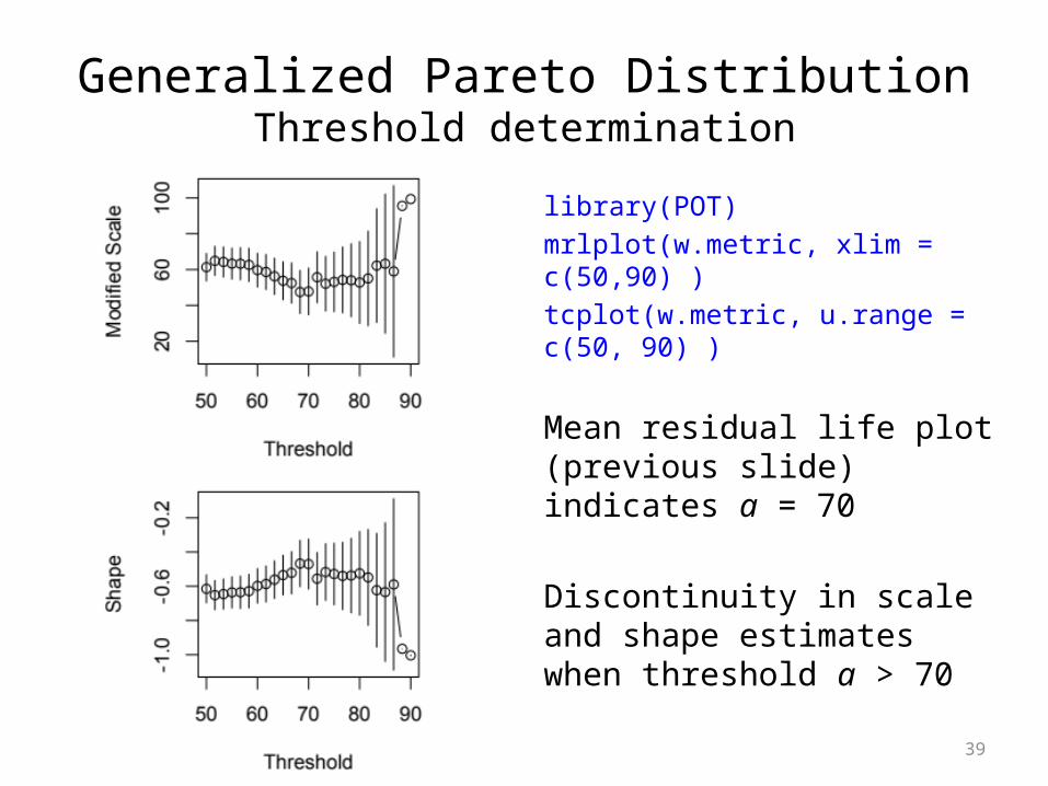
Generalized Pareto DistributionThreshold determination

library(POT)mrlplot(w.metric, xlim = c(50,90) )tcplot(w.metric, u.range = c(50, 90) )

Mean residual life plot (previous slide) indicates a = 70

Discontinuity in scale and shape estimates when threshold a > 70

40

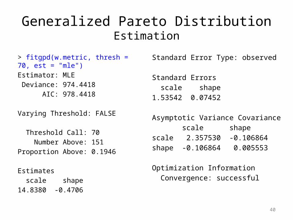
Generalized Pareto DistributionEstimation

> fitgpd(w.metric, thresh = 70, est = "mle")Estimator: MLE Deviance: 974.4418 AIC: 978.4418

Varying Threshold: FALSE

Threshold Call: 70 Number Above: 151 Proportion Above: 0.1946

Estimates scale shape 14.8380 -0.4706

Standard Error Type: observed

Standard Errors scale shape 1.53542 0.07452

Asymptotic Variance Covariance scale shape scale 2.357530 -0.106864shape -0.106864 0.005553

Optimization Information Convergence: successful

41

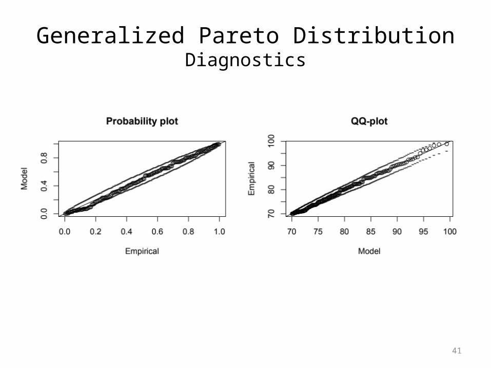
Generalized Pareto DistributionDiagnostics

42

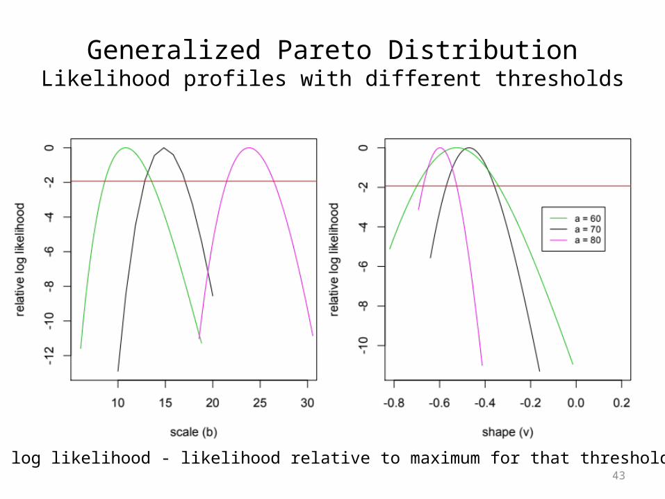
Generalized Pareto DistributionLikelihood profiles

43

Generalized Pareto DistributionLikelihood profiles with different thresholds

relative log likelihood - likelihood relative to maximum for that threshold value

44

Generalized Pareto DistributionEmpirical and Estimated

Comparison of empirical (no observed strikes) and GPD model estimates for a = 70

• Since 2000, 2 confirmed strikes

• GPD provides better characterization of risk

EmpiricalGPD

45

Generalized Pareto DistributionReturn Level

Return level – how many encounters where whales are less than 300m until a strike?

Conditional return level of approx. 500

Absolute return level of approx. 2500 (1 in 5 encounters has an encounter < 300m)

46

Summary: GEV and EVT

• Generalized Extreme Value (GEV) distribution– Used for block maxima, e.g., maximum sea-level

per year– Data loss due to only block maxima

• Generalized Pareto Distribution (GPD)– Used for points over a threshold– All exceedances above some limit are used– Question about how to deal with selecting a

threshold value

47

Additional ResourcesBooks and Papers

Coles, S. 2001. An Introduction to Statistical Modelling of Extreme Values. Springer Series in Statistics. London.

McNeil, A. J., Frey, R., & Embrechts, P. 2005. Quantitative risk management: concepts, techniques, and tools. Princeton University Press.

Embrechts, P. 1997. Modelling extremal events: for insurance and finance (Vol. 33). Springer.

Bayesian GPD ModelingColes, S. and L. Pericchi. 2003. Anticipating catastrophes through extreme value modeling. Applied Statistics 52(4): 405–416.

Jagger. T. H. and J. B. Elsne 2004. Climatology models for extreme hurricane winds near the United States. Journal of Climate 19: 3220-3236.

48

Additional ResourcesFitting models in R and BUGS

A few R packages• Points over Threshold (POT)• Extreme Value Distributions (evd)• extRemes• Quantitative Risk Management (QRM)• evdbayesBUGS• OpenBUGS – GEV and GPD• WinBUGS/JAGS – GPD with 1’s trick