Discussion PaperDeutsche BundesbankNo 16/2019

Extreme inflation andtime-varying consumption growth

Ilya Dergunov(Goethe University Frankfurt)

Christoph Meinerding(Deutsche Bundesbank)

Christian Schlag(Goethe University Frankfurt)

Discussion Papers represent the authors‘ personal opinions and do notnecessarily reflect the views of the Deutsche Bundesbank or the Eurosystem.

Editorial Board: Daniel Foos

Thomas Kick

Malte Knüppel

Vivien Lewis

Christoph Memmel

Panagiota Tzamourani

Deutsche Bundesbank, Wilhelm-Epstein-Straße 14, 60431 Frankfurt am Main,

Postfach 10 06 02, 60006 Frankfurt am Main

Tel +49 69 9566-0

Please address all orders in writing to: Deutsche Bundesbank,

Press and Public Relations Division, at the above address or via fax +49 69 9566-3077

Internet http://www.bundesbank.de

Reproduction permitted only if source is stated.

ISBN 978–3–95729–583–5 (Printversion)

ISBN 978–3–95729–584–2 (Internetversion)

Non-technical summary

Research Question

Whether and how changes in expected inflation affect expectations concerning the real

economy has always been an intensely debated question. In this paper, we provide a new

perspective on this issue by embedding inflation in one of the workhorse models of real

equilibrium asset pricing, namely the long-run risk framework. This class of models has

been widely applied in the literature, but has rarely been extended towards the pricing of

nominal assets.

Results

We find that, when the long-run risk model is augmented by inflation, time variation in

expected consumption growth can explain time variation in the stock-bond return corre-

lation. Key to this finding is the empirical observation that extreme expected inflation –

both very high and very low – is linked to low average consumption growth. Depending on

the state of the economy, an increase in expected inflation can be either a good or a bad

signal for real expected consumption growth, and this signalling channel drives changes

in the return correlation between real and nominal assets. As a validation of our channel,

we also find that the long-run risk variable that we extract exclusively from macro data

via the estimation of our model is highly correlated with long-run risk proxies suggested

in the literature, with the important difference that those are usually extracted from asset

price data.

Contribution

We show that one of the workhorse real equilibrium asset pricing models can explain

the stock-bond return correlation when we properly condition on inflation as a signal for

expected consumption growth. The probability of being in a low expected consumption

growth state is closely linked to implicit long-run risk variables in the literature that

have been extracted from asset prices. All the aforementioned results are derived from

macro data only. This is key for our analysis, since asset price data have the potential to

severely confound a macro estimation by imposing the strong parametric structure of an

asset pricing model.

Nichttechnische Zusammenfassung

Fragestellung

Ob und wie sich Anderungen der erwarteten Inflation auf realwirtschaftliche Erwartun-

gen auswirken, ist nach wie vor eine umstrittene Frage. In diesem Papier beleuchten

wir dieses Thema aus einer neuen Perspektive, indem wir Inflation in ein Asset-Pricing-

Gleichgewichtsmodell mit langfristigen Konsumrisiken einbetten. Diese Klasse von Asset-

Pricing-Modellen gehort inzwischen zum Standard in der Literatur, ist aber bislang kaum

auf die Bewertung von nominalen Wertpapieren angewendet worden.

Ergebnisse

Wir zeigen, dass die zeitliche Variation im erwarteten Konsumwachstum die zeitliche Va-

riation in der Korrelation zwischen Aktien- und Anleihenrenditen erklaren kann, sofern

das reale Standard-Modell um Inflation erweitert wird. Der entscheidende Schritt ist hier-

bei die empirische Beobachtung, dass extreme erwartete Inflation - sowohl sehr hohe als

auch sehr niedrige - mit einem niedrigen durchschnittlichen Konsumwachstum einhergeht.

Abhangig vom Zustand der Volkswirtschaft kann ein Anstieg der erwarteten Inflation da-

mit entweder als positives oder als negatives Signal fur das reale erwartete Konsumwachs-

tum interpretiert werden. Dies fuhrt zu Zeitvariation in der Korrelation der Renditen von

realen und nominalen Wertpapieren. Um diesen Mechanismus zu validieren, zeigen wir,

dass die Variable fur langfristiges Konsumrisiko, die wir ausschließlich aus Makrodaten

durch die Schatzung unseres Modells extrahieren, in hohem Maße mit ahnlichen in der

Literatur vorgeschlagenen Variablen korreliert, mit dem wichtigen Unterschied, dass jene

normalerweise aus Wertpapierpreisdaten extrahiert werden.

Beitrag

Wir zeigen, dass eines der wichtigsten realen Asset-Pricing-Gleichgewichtsmodelle zeitli-

che Variation in der Korrelation von Aktien- und Anleiherenditen erklaren kann, wenn

wir Inflation als Signal fur erwartetes Konsumwachstum angemessen berucksichtigen.

Die Wahrscheinlichkeit eines niedrigen erwarteten Konsumwachstums ist eng mit im-

pliziten Variablen fur langfristiges Konsumrisiko verknupft, die in der Literatur bisher

zumeist aus Wertpapierpreisen extrahiert wurden. Unsere Schatzung basiert ausschließ-

lich auf makrookonomischen Daten. Dies ist fur unsere Analyse von zentraler Bedeutung,

da Asset-Preisdaten das Potenzial haben, die makrookonomischen Implikationen eines

Asset-Pricing-Modells stark zu beeintrachtigen, wenn zu strenge parametrische Annah-

men getroffen werden.

Deutsche Bundesbank Discussion Paper No 16/2019

Extreme Inflation and Time-Varying ConsumptionGrowth∗

Ilya DergunovGoethe University Frankfurt

Christoph MeinerdingDeutsche Bundesbank

Christian SchlagGoethe University Frankfurt

Abstract

In a parsimonious regime switching model, expected consumption growth varies overtime. Adding inflation as a conditioning variable, we uncover two states in whichexpected consumption growth is low, one with high and one with negative expectedinflation. Embedded in a general equilibrium asset pricing model with learning,these dynamics replicate the observed time variation in stock return volatilities andstock-bond return correlations. Furthermore, they provide an alternative way tocome up with a measure of time-varying disaster risk in the spirit of Wachter (2013).Our findings imply that both the disaster and the long-run risk paradigm can beextended towards explaining movements in the stock-bond return correlation.

Keywords: Long-run risk, inflation, recursive utility, filtering, disaster risk

JEL classification: E31, E44, G12.

∗Contact address: Deutsche Bundesbank, Research Centre, Wilhelm-Epstein-Str. 14, 60431 Frankfurtam Main, Germany. E-mail: christoph.meinerding@bundesbank.de. We would like to thank the seminarparticipants and colleagues at Goethe University, Deutsche Bundesbank, Wharton, BI Oslo, IWH Halle,SNB and OeNB as well as the participants of the WFA 2018 Coronado, SGF 2018, German EconomistsAbroad Conference 2017, Paris December Finance Meeting 2017, DGF 2017, ESSFM Gerzensee 2017,MFA 2017 , AFFI 2017, and the 2017 Colloquium on Financial Markets in Cologne for their commentsand suggestions. Special thanks go to Angela Abbate (discussant), Geert Bekaert, Fernando Duarte,Stefan Eichler (discussant), Philipp Illeditsch, Jan Kragt (discussant), Mattia Landoni, Sydney Ludvig-son, Emanuel Monch, Olesya Grishchenko (discussant), Philippe Mueller, Athanasios Orphanides, MarcelPriebsch, Dongho Song (discussant), Marta Szymanowska, Jules van Binsbergen, Jessica Wachter (dis-cussant), Todd Walker, Rudiger Weber (discussant), Amir Yaron, and to Franziska Schulte and IliyaKaraivanov for excellent research assistance. A previous version of this paper was circulated under thetitle “Extreme inflation and time-varying disaster risk”. We gratefully acknowledge research and financialsupport from the Research Center SAFE, funded by the State of Hessen initiative for research LOEWE.This work represents the authors’ personal opinions and does not necessarily reflect the views of theDeutsche Bundesbank.

1 Introduction

Whether and how changes in expected inflation affect expectations concerning the realeconomy has always been an intensely debated question. In this paper, we provide anew perspective on this issue by embedding inflation in one of the workhorse models ofequilibrium asset pricing, namely the long-run risk framework. We find that, when aregime-switching model featuring long-run risk is augmented by inflation, time variationin expected consumption growth can explain time variation in the stock-bond returncorrelation and in aggregate stock market volatility.

Key to this finding is the empirical observation that extreme expected inflation –both very high and very low – is linked to low average consumption growth. Includinginflation in a parsimonious regime switching model thus significantly affects the estimateddynamics of the conditional mean of consumption growth relative to a model based onconsumption only. We embed the estimated regime-switching dynamics in an otherwisestandard equilibrium asset pricing model with learning, thereby extending the long-runrisk framework towards explaining the joint dynamics of real and nominal assets. Thisvery stylized model allows us to match, among other things, the empirically observedtime-varying nature of the return correlation between stocks and nominal bonds. As afurther validation of our channel, we also find that the long-run risk variable that weextract (exclusively) from macro data via the estimation of the regime-switching model ishighly correlated with long-run risk proxies suggested in the literature, with the importantdifference that those are usually reverse-engineered from asset price data.

Long-run risk asset pricing models rest on the key assumption that the conditionaldistribution of consumption growth, in particular its mean, is time-varying. Followingthe seminal publication of Bansal and Yaron (2004), a lot of papers dealt with the issueof detecting such time variation.1 In this paper, we take a step back and document theexistence of long-run risk by fitting a parsimonious regime-switching model for consump-tion growth to standard quarterly NIPA aggregate consumption data. We show that thehypothesis of constant expected consumption growth can be rejected at any conventionalsignificance level.

Based on this, our paper then makes the following four key contributions. First,augmenting the time series model by inflation as a second variable, we detect two statesin which expected consumption growth is low, one with very high expected inflation (so-called “stagflation”) and one with negative expected inflation (“deflation”). The fact thatthere are two very different states with low expected consumption growth turns out to beimportant for asset pricing.

Second, by embedding the estimated dynamics in a standard general equilibrium assetpricing model with recursive preferences and learning, we show that imperfect informa-tion about expected consumption growth drives time variation in aggregate stock marketvolatility and in the stock-bond correlation when we properly condition on inflation as asignal.

Third, the probability of being in a low expected consumption growth state that we

1A nice synopsis of arguments against or in favor of long-run risk is given by the two competing papersof Beeler and Campbell (2012) and Bansal, Kiku, and Yaron (2012), respectively. Recent advances weremade by Schorfheide, Song, and Yaron (2018), who document and analyze the persistent component inexpected consumption growth employing sophisticated Bayesian mixed frequency techniques.

1

obtain from our macro estimation with consumption and inflation data tracks the histori-cal price-earnings ratio of US equity well. It is therefore closely linked to implicit long-runrisk variables that have been obtained through reverse engineering from asset prices inthe literature. As an example, we provide an alternative derivation and interpretation ofthe “time-varying disaster risk” presented in Wachter (2013), which is one prime exampleof such a variable.

Finally, we wish to emphasize that we produce all the aforementioned results withinan rather simple setup, where no asset price data are used in the estimation. This is keyfor our analysis, since asset price data have the potential to severely confound a macroestimation, e.g., via certain moment conditions to represent the parametric structure ofan asset pricing model included in an application of GMM.

We now give some more details on our contributions. The Markov regime switchingmodel is a simple and convenient representation of the case of time-varying expectedconsumption growth. The estimation gives two states for the conditional mean, and aWald test rejects the hypothesis of the conditional means being equal at any conventionalsignificance level. We then add inflation as a second variable, and in this extended model,expected inflation and expected consumption growth are related in a nonlinear way: bothextremely high and extremely low expected inflation are coupled to low expected con-sumption growth, and in particular the possibility of negative inflation is an importantdriver of many of our results.

The recent literature on long-run risk in asset pricing, e.g. Wachter (2013), puts anemphasis on the link between time variation in the conditional distribution of consumptiongrowth and time variation in second moments of returns. Motivated by the time series re-sults above, we embed the fundamental dynamics into a state-of-the-art equilibrium assetpricing model, where the representative investor is equipped with recursive preferences.Given the usual values for risk aversion and the elasticity of intertemporal substitution,the substitution effect dominates, so that prices are decreasing in the amount of aggregaterisk.

In line with papers like Detemple (1986), or Croce, Lettau, and Ludvigson (2012), wemake the assumption that the representative investor knows the structural parameters ofthe model, but cannot observe the true state and thus can only filter the respective proba-bilities from the data. Given our estimation, extreme (high or low) inflation observationsserve as a useful signal, which allows to better infer the time-varying probability of verylow or even negative consumption growth. The fact that low real growth can be linkedto high or low expected inflation is key to producing a time-varying stock-bond returncorrelation. When very high expected inflation occurs together with low expected realgrowth, both bonds and stocks will tend to have negative returns, resulting in a positivecorrelation. On the other hand, low growth expectations in periods with low expectedinflation will lead to negative equity returns, but positive bond returns, implying a nega-tive correlation. Stated differently, the long-run risk paradigm can be extended towardsthe time-varying nature of the stock-bond return correlation when the signaling role ofinflation is taken into account properly.

We test the asset pricing implications of our model by feeding it with the empiricaltime series of observed consumption growth and inflation and then pricing stocks andbonds using our model-implied pricing kernel. We then compare the dependence of stockreturn volatilities and stock-bond correlations on the filtered probabilities in the model

2

and the data. In both model and real data the stock-bond return correlation is positivelyand significantly linked to the probability of being in the high-inflation state, while for thedeflationary state we find exactly the opposite. The model also qualitatively matches twokey results in Wachter (2013). First, stock market volatility is increasing in the (filtered)probability of being in a bad consumption growth state. Second, the relation betweenstock market volatility and this probability is nonlinear both in the model and in thedata.

Finally, our approach using only macroeconomic data also offers a nice alternativederivation of the state variable “time-varying disaster probability” that Wachter (2013)has produced in her paper. The correlation between her variable and our filtered probabil-ity of being in a bad consumption growth state is 0.88, and this co-movement is mirroredin the close co-movement between the dividend-price ratio in the data and in our model.Although there is no explicit role for disaster risk in our model, we choose this time seriesfor comparison because its interpretation as a “probability” is much closer to the basicstate variables in our model than, for instance, estimated time series of mean consump-tion growth. We draw the tentative conclusion that the “implied disaster probability” inWachter (2013), which is obtained through a transformation of the historical dividend-price ratio of the S&P 500, is closely linked to time variation in expected consumptiongrowth, which we estimate from consumption and inflation data alone. This interpre-tation also reinforces the findings of Branger, Kraft, and Meinerding (2016) who arguethat disaster risk and long-run risk are intertwined in historical data. The episodes ofhigh marginal utility which Wachter (2013) labels as episodes of elevated disaster riskare characterized by low expected consumption growth according to our Markov chainestimation.

We close the paper with a number of robustness checks concerning both the estima-tion and the asset pricing model. First, we show that a Markov switching model forconsumption growth only (i.e., without inflation) cannot replicate the time series of thedividend-price ratio. Second, our results do not depend on expected consumption growthbeing particularly low (high) in one of the two bad (good) states. A model where expectedgrowth is constrained to be the same in the two good and in the two bad states, respec-tively, delivers qualitatively the same results. Third, additional analyses with subsamples,with GDP growth instead of consumption growth, or with monthly consumption data alsolargely confirm our findings.2 Fourth, on the asset pricing side, we document that our twomajor assumptions – recursive preferences and learning from inflation observations – areboth key to generating our main results. In a nested model with CRRA preferences, theregression of correlations on state variables delivers coefficients whose signs are oppositeto the data. A nested model in which the state of the economy is perfectly observable hasproblems to generate the recently observed negative correlation in the first place.

2We also estimate the Markov chain model on a long sample of annual data and identify a deflationarystate there as well. As is clear from the discussion above, the identification of a deflationary state iscrucial to match the asset price data. In our benchmark estimation, this identification largely restson the deflation observations during the Financial Crisis in 2008. However, there are also deflationaryepisodes in pre-war data, which are not contained in our benchmark sample of quarterly data starting in1947.

3

2 Related Literature

Our paper contributes to and links two major strands of literature, namely the assetpricing literature about inflation as a priced risk factor and the asset pricing literaturefeaturing long-run risk and its empirical estimation. We do not aim at giving a full reviewof the numerous papers in the latter field. Contributions there have been made by Bansaland Yaron (2004), Bansal, Kiku, and Yaron (2016) Beeler and Campbell (2012), Bansalet al. (2012), Constantinides and Ghosh (2011), Ortu, Tamoni, and Tebaldi (2013), andSchorfheide et al. (2018), among many others.

Concerning equilibrium asset pricing with inflation risk, we mostly build on the follow-ing papers. Bansal and Shaliastovich (2013) propose a long-run risk model with expectedinflation and expected growth as risk factors and use it to explain the empirically observedpredictability patters in bond and foreign exchange returns. Eraker (2008) proposes anaffine jump-diffusion model with jumps in consumption volatility. Eraker, Shaliastovich,and Wang (2016) discuss a long-run risk model with inflation as a risk factor, but theirfocus is on differences between durable and non-durable consumption and their implica-tions for equity and bond prices in these sectors. Ehling, Gallmeyer, Heyerdahl-Larsen,and Illeditsch (2018) consider heterogeneous agents who disagree about inflation, and theauthors show that this disagreement increases yields and yield volatilities at all maturi-ties. Burkhardt and Hasseltoft (2012) propose a model with recursive utility, inflationand long-run risk similar to ours, but, given the way in which the authors introduce in-flation risk premia, the asset pricing results seem to a certain degree hardwired into themodel. We consider our approach less restrictive in terms of the specification of inflationand consumption growth. Piazzesi and Schneider (2006) discuss the role of inflation as asignal about future consumption growth, but they focus on the term structure of (nominaland real) interest rates and do not address time variation in the stock-bond correlation.

Song (2017) studies an endowment economy model with recursive preferences, a regime-switching Taylor rule, and a time-varying inflation target. Campbell, Pflueger, and Viceira(2018) analyze the stock-bond correlation in a New Keynesian production economy withhabit formation preferences and monetary policy regimes. Complementary to our paper,Constantinides and Ghosh (2017) assess the ability of several macroeconomic predic-tor variables to improve the performance of consumption-based equilibrium asset pricingmodels, and they find that inflation data helps to generate the (non-)predictability ofprice-dividend ratios by cash flow growth rates. In all these papers, however, asset pricedata is used to calibrate or estimate the model. Ermolov (2018) estimates an externalhabit model with macroeconomic data only, but his explanation of time variation in thestock-bond correlation is very different from ours. He assumes that consumption andinflation can be hit by two different shocks labeled as supply and demand shocks, whereaswe rely on different regimes for expected growth rates.

David and Veronesi (2013) propose Markov switching dynamics for fundamentals, butthey assume a model featuring a representative agent with time-additive CRRA prefer-ences who suffers from bounded rationality in the form of money illusion in the spirit ofBasak and Yan (2010). Since their GMM estimation relies on asset price data, it deliversquite different dynamics for the fundamentals compared to our estimation, most impor-tantly state-independent expected consumption growth. This is because the estimationtargets empirical dividend-price ratios and thus has to shut down the intertemporal sub-

4

stitution channel, i.e. there is no role for long-run risk in their estimated model. We showin our empirical results that the hypothesis of constant expected consumption growth canbe rejected at any conventional significance level if the estimation is based on macro dataonly.

Boons, de Roon, Duarte, and Szymanowska (2017) provide empirical evidence for in-flation risk being priced in the cross-section of stock returns. Their paper can be viewedas complementary to ours, since the market price of inflation risk estimated from thecross-section of stock returns switches sign and is linked to the stock-bond correlationin the data. It can be considered a stylized fact that the correlation between inflationand other variables can change the sign of the stock-bond correlation, and we provide amodel-theoretic explanation for this result. Other papers in this area include Schmelingand Schrimpf (2011), Balduzzi and Lan (2016), Campbell, Sunderam, and Viceira (2017),Hasseltoft (2012), Ang and Ulrich (2012), and Marfe (2015), to name just a few. Baele,Bekaert, and Inghelbrecht (2010) empirically analyze the determinants of the stock-bondreturn comovement. Fleckenstein, Longstaff, and Lustig (2016) study the pricing of de-flation risk using market prices of inflation-linked derivatives.

Through the re-interpretation of our state variables as measuring time-varying disasterrisk, our paper is also related to this area of research. Rietz (1988) and Barro (2006, 2009)rationalize a high equity premium in the disaster risk framework. Extensions of their basicmodel have been studied by Chen, Joslin, and Tran (2012) and Julliard and Ghosh (2012),among others. Constantinides (2008) criticizes that historically consumption disastersrather unfold over several years instead of just one point in time. Similarly to the critiqueof Constantinides (2008), the assumption of extreme jumps is also questioned by Backus,Chernov, and Martin (2011). As a response, Branger et al. (2016) combine disaster riskand long-run risk and show that the equity premium puzzle can still be solved withmulti-period disasters. Similarly, Gabaix (2012), Wachter (2013), and Tsai and Wachter(2015) analyze models with time-varying jump intensities and recursive preferences. Ourresults imply that the disaster risk paradigm may be extended towards an explanation ofthe time-varying stock-bond return correlation, when the effect of inflation on real assetprices is captured properly. Finally, in this regard, our paper may also contribute to thediscussion about “dark matter” in asset prices started by Chen, Dou, and Kogan (2017)in the sense that a large fraction of this dark matter may be attributed to uncertaintyabout extreme inflation.

3 Fundamental Dynamics

3.1 Consumption and inflation

The two fundamental sources of risk in our model are aggregate consumption and inflation.In the baseline version without inflation, we assume that log aggregate real consumption,lnC, follows the process

d lnCt = µC(St)dt+ σCdWCt . (1)

WC is a standard Wiener process, the volatility σC is constant. The conditional drift rateµC(St) is stochastic and follows a continuous-time Markov chain whose current state isdenoted by St. There are n states (indexed by i = 1, . . . , n), with state-dependent drifts

5

µCi . The Markov chain transitions are governed by counting processes whose intensitiesare collected in the (n× n)-matrix Λ = (λij)i,j=1,...,n. Following the usual convention, wedefine the diagonal elements λii := −

∑j 6=i λij so that the rows of Λ sum to 0. In our

benchmark empirical case, we will have n = 2.In the full model, the joint dynamics of log aggregate real consumption and of the log

price level π are given as

d lnCt = µC(St)dt+ σC(√

1− ρ2dWCt + ρdW π

t

)dπt = µπ(St)dt+ σπdW π

t .(2)

Here WC and W π are the (independent) components of a standard bivariate Wienerprocess. The dynamics in (2) imply that the increments to lnC and to π are correlatedwith correlation parameter ρ. The volatilities σC and σπ are assumed constant. Theconditional drift rates µC(St) and µπ(St) now follow a bivariate continuous-time Markovchain whose current state is again denoted by St. Keeping the rest of the notation asabove, the number of states in the full model will later turn out to be n = 4.

We will often use the vector representation of the above dynamics, which can bewritten as (

d lnCtdπt

)= µ(St) dt+ Σ dWt

with

µ(St) =

(µC(St)µπ(St)

), Σ =

(σC√

1− ρ2 σCρ0 σπ

), dWt =

(dWC

t

dW πt

).

3.2 Markov chain estimation

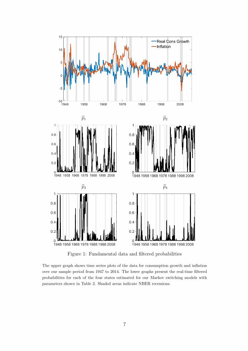
To estimate the dynamics of the fundamentals we use quarterly real consumption growthrates from NIPA and quarterly inflation rates constructed according to the Piazzesi andSchneider (2006) mechanism.3 Our sample period ranges from 1947Q1 to 2014Q1 andrepresents the longest period for which quarterly data are available.4 The upper graph inFigure 1 shows time series plots of the data.

Based on these data for consumption and inflation we estimate the two models (1) and(2) using maximum likelihood.5 We assume a constant variance-covariance matrix andonly allow for time-varying drifts. Instead of the transition intensities Λ, the estimationgives us an (n × n)-matrix Q = (qij)i,j=1...,n of transition probabilities, which are linkedto the intensities via λij = − log(1 − qij) for j 6= i. The diagonal elements qii of thetransition probability matrix are set such that the rows sum to 1. Standard errors for the

3The choice of this inflation time series is in line with the literature on consumption-based asset pricingwith a focus on inflation risk, e.g. Song (2017), David and Veronesi (2013), Burkhardt and Hasseltoft(2012). For a detailed discussion of this issue, we refer the reader to Piazzesi and Schneider (2006).

4We have performed the estimation also with alternative samples to compare our findings to thosestated in other papers. These results are discussed in Section 6.4. Besides, we have also estimated variousconstraint versions of the models in which the number of parameters is reduced. This does not changeany of our results qualitatively. Details on these constraint models are presented in Section 6.5.

5For details about the estimation procedure, see Online Appendix A.

6

p1 p2

p3 p4

Figure 1: Fundamental data and filtered probabilities

The upper graph shows time series plots of the data for consumption growth and inflation

over our sample period from 1947 to 2014. The lower graphs present the real-time filtered

probabilities for each of the four states estimated for our Markov switching models with

parameters shown in Table 2. Shaded areas indicate NBER recessions.

7

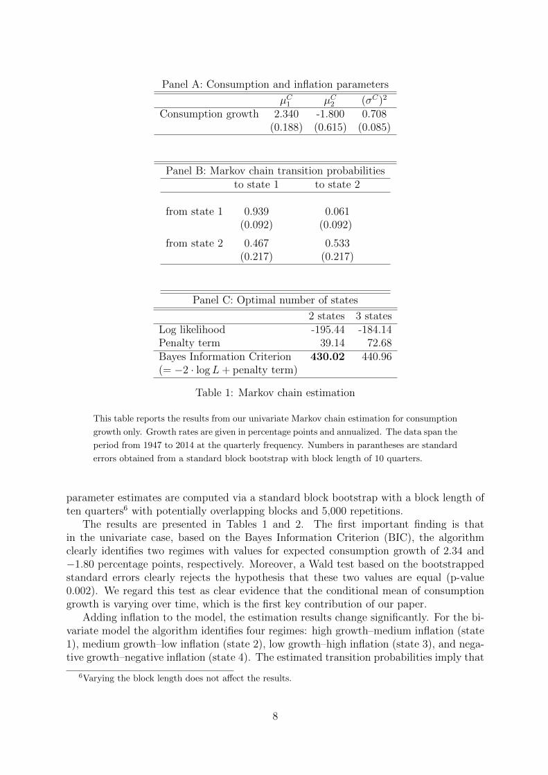
Panel A: Consumption and inflation parameters

µC1 µC2 (σC)2

Consumption growth 2.340 -1.800 0.708(0.188) (0.615) (0.085)

Panel B: Markov chain transition probabilitiesto state 1 to state 2

from state 1 0.939 0.061(0.092) (0.092)

from state 2 0.467 0.533(0.217) (0.217)

Panel C: Optimal number of states

2 states 3 statesLog likelihood -195.44 -184.14Penalty term 39.14 72.68Bayes Information Criterion 430.02 440.96(= −2 · logL+ penalty term)

Table 1: Markov chain estimation

This table reports the results from our univariate Markov chain estimation for consumption

growth only. Growth rates are given in percentage points and annualized. The data span the

period from 1947 to 2014 at the quarterly frequency. Numbers in parantheses are standard

errors obtained from a standard block bootstrap with block length of 10 quarters.

parameter estimates are computed via a standard block bootstrap with a block length often quarters6 with potentially overlapping blocks and 5,000 repetitions.

The results are presented in Tables 1 and 2. The first important finding is thatin the univariate case, based on the Bayes Information Criterion (BIC), the algorithmclearly identifies two regimes with values for expected consumption growth of 2.34 and−1.80 percentage points, respectively. Moreover, a Wald test based on the bootstrappedstandard errors clearly rejects the hypothesis that these two values are equal (p-value0.002). We regard this test as clear evidence that the conditional mean of consumptiongrowth is varying over time, which is the first key contribution of our paper.

Adding inflation to the model, the estimation results change significantly. For the bi-variate model the algorithm identifies four regimes: high growth–medium inflation (state1), medium growth–low inflation (state 2), low growth–high inflation (state 3), and nega-tive growth–negative inflation (state 4). The estimated transition probabilities imply that

6Varying the block length does not affect the results.

8

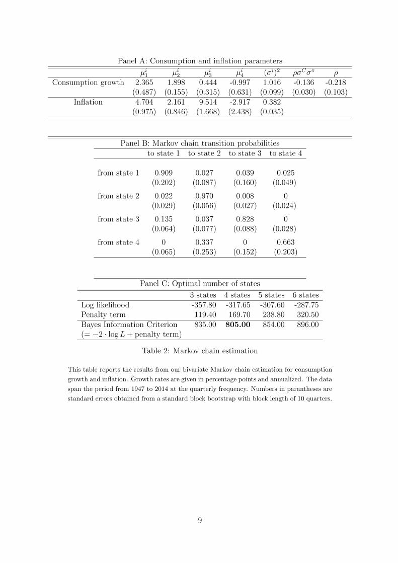
Panel A: Consumption and inflation parameters

µi1 µi2 µi3 µi4 (σi)2 ρσCσπ ρConsumption growth 2.365 1.898 0.444 -0.997 1.016 -0.136 -0.218

(0.487) (0.155) (0.315) (0.631) (0.099) (0.030) (0.103)Inflation 4.704 2.161 9.514 -2.917 0.382

(0.975) (0.846) (1.668) (2.438) (0.035)

Panel B: Markov chain transition probabilitiesto state 1 to state 2 to state 3 to state 4

from state 1 0.909 0.027 0.039 0.025(0.202) (0.087) (0.160) (0.049)

from state 2 0.022 0.970 0.008 0(0.029) (0.056) (0.027) (0.024)

from state 3 0.135 0.037 0.828 0(0.064) (0.077) (0.088) (0.028)

from state 4 0 0.337 0 0.663(0.065) (0.253) (0.152) (0.203)

Panel C: Optimal number of states

3 states 4 states 5 states 6 statesLog likelihood -357.80 -317.65 -307.60 -287.75Penalty term 119.40 169.70 238.80 320.50Bayes Information Criterion 835.00 805.00 854.00 896.00(= −2 · logL+ penalty term)

Table 2: Markov chain estimation

This table reports the results from our bivariate Markov chain estimation for consumption

growth and inflation. Growth rates are given in percentage points and annualized. The data

span the period from 1947 to 2014 at the quarterly frequency. Numbers in parantheses are

standard errors obtained from a standard block bootstrap with block length of 10 quarters.

9

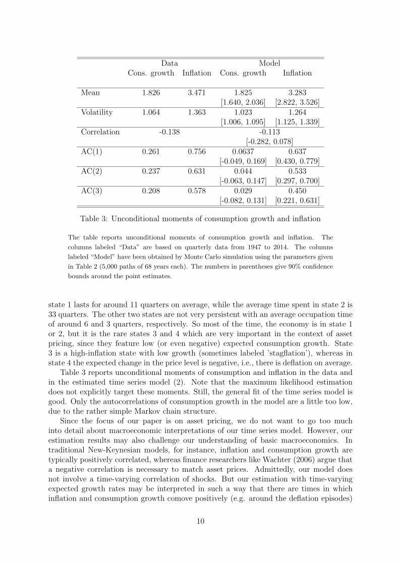
Data ModelCons. growth Inflation Cons. growth Inflation

Mean 1.826 3.471 1.825 3.283[1.640, 2.036] [2.822, 3.526]

Volatility 1.064 1.363 1.023 1.264[1.006, 1.095] [1.125, 1.339]

Correlation -0.138 -0.113[-0.282, 0.078]

AC(1) 0.261 0.756 0.0637 0.637[-0.049, 0.169] [0.430, 0.779]

AC(2) 0.237 0.631 0.044 0.533[-0.063, 0.147] [0.297, 0.700]

AC(3) 0.208 0.578 0.029 0.450[-0.082, 0.131] [0.221, 0.631]

Table 3: Unconditional moments of consumption growth and inflation

The table reports unconditional moments of consumption growth and inflation. The

columns labeled “Data” are based on quarterly data from 1947 to 2014. The columns

labeled “Model” have been obtained by Monte Carlo simulation using the parameters given

in Table 2 (5,000 paths of 68 years each). The numbers in parentheses give 90% confidence

bounds around the point estimates.

state 1 lasts for around 11 quarters on average, while the average time spent in state 2 is33 quarters. The other two states are not very persistent with an average occupation timeof around 6 and 3 quarters, respectively. So most of the time, the economy is in state 1or 2, but it is the rare states 3 and 4 which are very important in the context of assetpricing, since they feature low (or even negative) expected consumption growth. State3 is a high-inflation state with low growth (sometimes labeled ’stagflation’), whereas instate 4 the expected change in the price level is negative, i.e., there is deflation on average.

Table 3 reports unconditional moments of consumption and inflation in the data andin the estimated time series model (2). Note that the maximum likelihood estimationdoes not explicitly target these moments. Still, the general fit of the time series model isgood. Only the autocorrelations of consumption growth in the model are a little too low,due to the rather simple Markov chain structure.

Since the focus of our paper is on asset pricing, we do not want to go too muchinto detail about macroeconomic interpretations of our time series model. However, ourestimation results may also challenge our understanding of basic macroeconomics. Intraditional New-Keynesian models, for instance, inflation and consumption growth aretypically positively correlated, whereas finance researchers like Wachter (2006) argue thata negative correlation is necessary to match asset prices. Admittedly, our model doesnot involve a time-varying correlation of shocks. But our estimation with time-varyingexpected growth rates may be interpreted in such a way that there are times in whichinflation and consumption growth comove positively (e.g. around the deflation episodes)

10

and other times in which they comove negatively (e.g. around the stagflation episodes).Moreover, our estimation is also in line with policy debates which document that negativeinflation (i.e., deflation) has re-entered the mindset of policymakers during the recent zerolower bound episode.

4 Asset Pricing Model

Long-run risk models in which expected consumption growth is time-varying are supposedto explain the time series behavior of asset prices and returns. In the following we willtherefore embed the dynamics estimated in the previous section into a state-of-the-artasset pricing model with recursive preferences and learning. Having inflation in the modelallows us to analyze the returns of stocks and nominal bonds jointly. The quantitativeresults presented in Section 5 are based on the parameter estimates from the benchmarkspecification in Table 2.7

4.1 Preferences

The economy is populated by an infinitely-lived representative investor with stochasticdifferential utility as introduced by Duffie and Epstein (1992b). The investor has theindirect utility function

J(Ct, p1t, . . . , pnt) = Et

[∫ ∞t

f(Cs, J(Cs, p1s, . . . , pns))ds

],

where the aggregator f is given by

f(C, J) =βC1− 1

ψ(1− 1

ψ

) [(1− γ)J

] 1θ−1− βθJ with γ 6= 1 and ψ 6= 1

γ, ψ, and β denote the degree of relative risk aversion, the elasticity of intertemporalsubstitution (EIS), and the subjective time preference rate, respectively. We define θ =1−γ1− 1

ψ

. The special case of time-separable CRRA preferences is represented by θ = 1, i.e.,

by γ = ψ−1. Throughout the paper, we assume γ = 10, ψ = 1.7, and β = 0.02.8 Withthis parameter choice, the agent has a preference for early resolution of uncertainty, sinceγ > ψ−1.

4.2 Filtering

We assume that the representative agent cannot observe St (and thus µC(St) and µπ(St))and has to filter her estimates from the data.9 We add learning first and foremost becausea full information economy does not generate reasonable time variation in price-dividend

7Alternative parameterizations are discussed in Section 6.8A nested version of our model with CRRA preferences (θ = 1) is discussed in Section 6.2.9As pointed out in the introduction and as it is standard in the literature, we assume that the

representative agent knows the structural parameters of the model, but does not know the current stateof the economy.

11

ratios. Incomplete information generates an additional layer of uncertainty that is key forour results. Besides the risk to switch to a bad state next period, which would also bepresent in a full information model, we add the uncertainty about the current regime andthus about the probability of switching to a bad regime.10

Mathematically, there are two filtrations, F and G, where F is generated by theprocesses (Ct)t, (πt)t and (St)t, whereas G ⊂ F is generated by the processes (Ct)t and(πt)t only. The conditional expectations of the drifts given the investor’s information, µCtand µπt , are given as

µCt = E[µC(St)|Gt

]=

n∑i=1

pitµCi

and

µπt = E [µπ(St)|Gt] =n∑i=1

pitµπi .

Here pit = E[1St=i|Gt

]denotes the subjective conditional probability of being in state i

at time t, and these conditional probabilities will serve as state variables in our economy.Since probabilities always sum up to 1, we will have n − 1 state variables p1, . . . , pn−1,whose support is the standard simplex in Rn−1.

Consumption growth and inflation realizations are observable and serve as a signal forthe aggregate state. The dynamics of pit follow from the so-called Wonham filter and aregiven by

dpit =

(λiipit +

∑j 6=i

λjipjt

)dt+ pit

[(µCiµπi

)−

n∑j=1

pjt

(µCjµπj

)]′(Σ′)−1

(dWC

t

dW πt

). (3)

with the “subjective” Brownian motions(dWC

t

dW πt

)= Σ−1

[(µCiµπi

)−

n∑j=1

pjt

(µCjµπj

)]dt+

(dWC

t

dW πt

).

A proof of the filtering equation based on Theorem 9.1 of Liptser and Shiryaev (2001)and a discussion of its properties are provided in Online Appendix B.

In the context of our analysis it is essential to note that the update in the estimatedprobability pi depends on both signals, i.e., on both realized consumption growth andrealized inflation. Inflation observations have an impact on the perceived probability ofbeing in state i and thus on the conditional expected consumption growth rate. This willbe the key driver for our asset pricing results described below.

The lower graphs in Figure 1 show the filtered estimates for the probabilities of thefour states, i.e., the estimates the investor would have computed based on information upto and including time t. These estimates are the key quantities analyzed in the followingsubsection. They will also serve as the explanatory variables in our regression analyses inSection 5. First of all, there is considerable variation in each of the four time series, i.e.,the probability of being in state i changes substantially over time. State 1 with the highest

10In Section 6.3 we compare our results to those from a nested model with full information, in whichthe agent can observe the economic state at any point in time.

12

expected real growth rate, but also above-average inflation is considered most likely bythe investor during the 1960s and much of the 1970s. The investor furthermore perceivesa high probability to be in the regime 2 with low inflation and stable growth for extendedperiods during the 1950s and much of the 1990s, but this probability is very low duringthe 1970s. Not surprisingly, there is a very high probability for the high inflation state 3during the latter period. The deflation state 4 is seen as very likely in the beginning ofthe sample right after the war and as well towards the end during the Great Recession.

4.3 Real Pricing Kernel and Wealth-Consumption Ratio

As shown in Duffie and Epstein (1992a), the real pricing kernel depends on the log wealth-consumption ratio v and is given by

ξt = C−γt e−βθt+(θ−1)

(t∫0

e−vudu+vt

).

The wealth-consumption ratio I ≡ ev depends on the estimated expected consumptiongrowth µC , and therefore in particular on the estimated probabilities pi. It solves anonlinear partial differential equation given in Online Appendix C.1. A proof and detailsconcerning the numerical solution using a Chebyshev polynomial approximation are alsopresented in Online Appendix C.1.

Given a solution for I, the pricing kernel has dynamics

dξtξt

= −βθdt− (1− θ)I−1 dt− γ dCtCt

+1

2γ2(σC)2dt− (1− θ)

n−1∑i=1

IpiIdpit

+1

2

n−1∑i=1

n−1∑j=1

(θ − 1)

[IpipjI

+ (θ − 2)

(IpiIpjI2

)]σpiσ

′pjdt− γ(θ − 1)

n−1∑i=1

IpiIσc,pi dt.

with the dynamics of dpit given in Equation (3). Importantly, shocks to the state variablespi affect the pricing kernel. Since these shocks are themselves driven by both consumptionand inflation observations, realized inflation indirectly enters the pricing kernel throughthe learning mechanism.

4.4 Pricing the Assets in the Economy

We are mainly interested in two types of assets, equity and nominal bonds. Equity isdefined as a claim to real dividends. When defining dividends, one has to be carefulnot to alter the informational setup of the model. Dividends are observable, and if theyprovided a non-redundant signal about the state of the economy, this would affect theinitial filtering problem. Technically, this requires the two systems of equations(

dWCt

dW πt

)= Σ−1

[(µCiµπi

)−

n∑j=1

pjt

(µCjµπj

)]dt+

(dWC

t

dW πt

)

13

and dWCt

dW πt

dWDt

= Σ−1∗

µCiµπiµDi

− n∑j=1

pjt

µCjµπjµDj

dt+

dWCt

dW πt

dWDt

to yield the same solution for dWC

t and dW πt . Here the superscript D denotes terms

related to dividend dynamics and Σ∗Σ′∗ is the covariance matrix of innovations to lnC, π

and lnD.The above condition for the redundance of dividends is satisfied by assuming

d lnDt = µdt+ φ

(n∑i=1

(µCi − µ)pit

)dt+ φσC

(√1− ρ2dWC

t + ρdW πt

).

Similar to Bansal and Yaron (2004), the deviation of the drift from its long-term averageµ is levered by a factor of φ, and like Bansal and Yaron (2004) we assume φ = 3.

Let ω denote the log price-dividend ratio. Starting from the Euler equation for theprice of the dividend claim, we can apply the Feynman-Kac formula to g(ξ,D, ω) ≡ ξDeω.This yields

Ag(ξ,D, ω)

g(ξ,D, ω)+ e−ω = 0,

where A denotes the infinitesimal generator. Using Ito’s Lemma, we can translate thisequation into a PDE for ω(p). This PDE, together with details regarding its derivation, isgiven in Online Appendix C.3. We solve this PDE again numerically using a Chebyshevapproximation.

A nominal bond pays off one unit of money at maturity T , which, in real terms, is

equal to exp(−∫ Ttdπsds

)= exp(πt− πT ). The price of a nominal bond at time t is thus

equal to

B$,Tt = Et

[ξTξt

exp(πt − πT )

].

Equivalently, one can define the nominal pricing kernel asξ$Tξt$≡ ξT

ξtexp(πt − πT ) and

rewrite the pricing formula as

B$,Tt = Et

[ξ$Tξt$

].

The dynamics of the nominal pricing kernel then follow from Ito’s lemma:

dξ$tξ$t

=dξtξt− dπt +

1

2d[π]t −

d[ξ, π]tξt

.

Importantly, the nominal risk-free short rate, i.e., the negative of the drift of ξ$, is notjust the sum of the real short rate and expected inflation, but involves the covariationbetween the real pricing kernel and inflation, d[ξ, π] (and the quadratic variation of π).The covariation is nonzero if inflation shocks affect the real pricing kernel, as they do inour model, and can be interpreted as an equilibrium inflation risk premium.

14

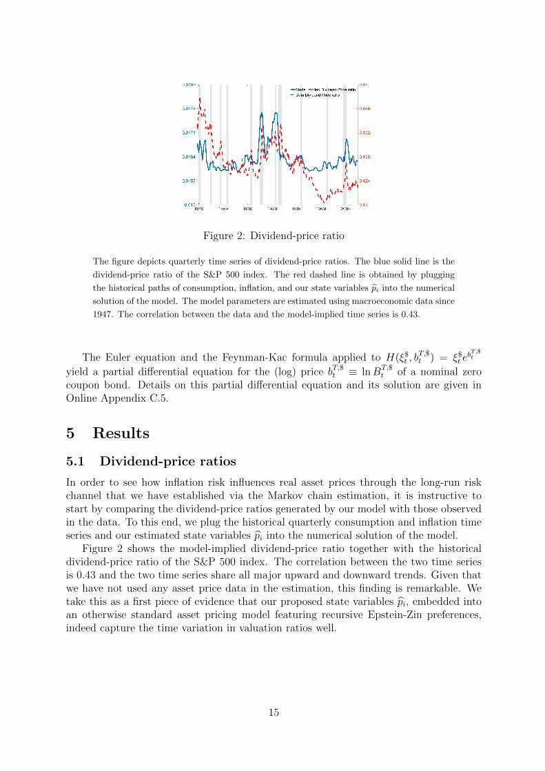
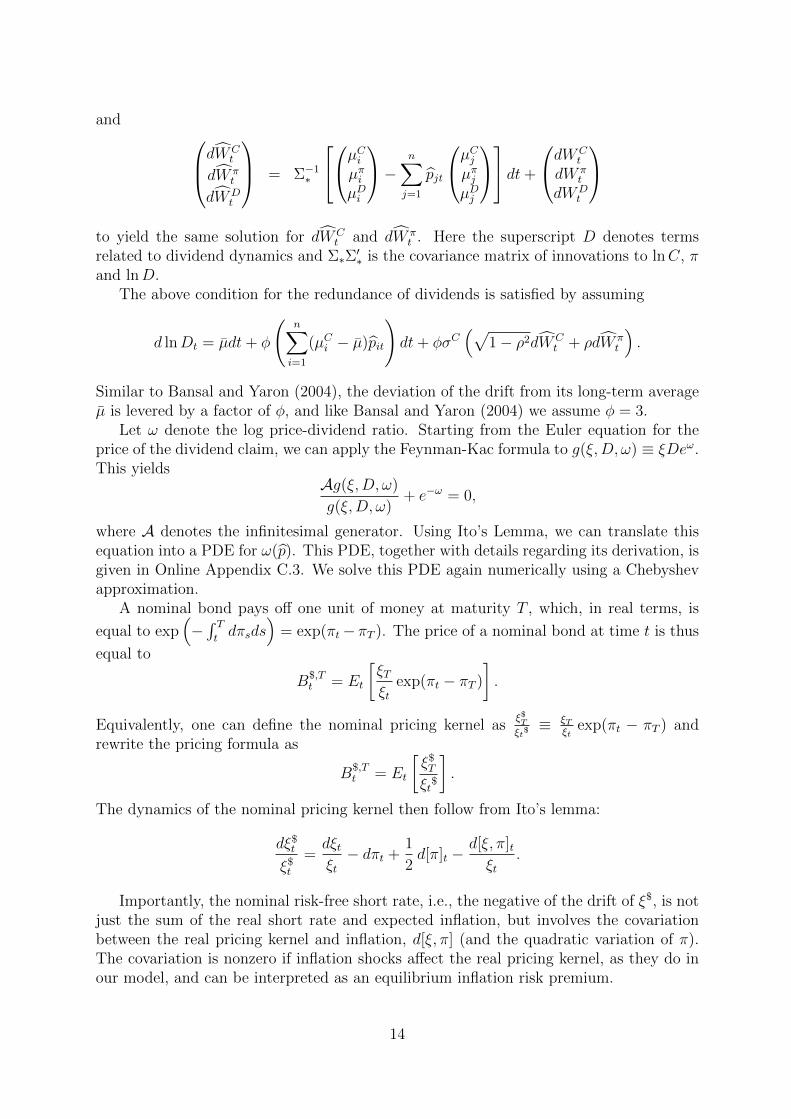
Figure 2: Dividend-price ratio

The figure depicts quarterly time series of dividend-price ratios. The blue solid line is the

dividend-price ratio of the S&P 500 index. The red dashed line is obtained by plugging

the historical paths of consumption, inflation, and our state variables pi into the numerical

solution of the model. The model parameters are estimated using macroeconomic data since

1947. The correlation between the data and the model-implied time series is 0.43.

The Euler equation and the Feynman-Kac formula applied to H(ξ$t , bT,$t ) = ξ$t e

bT,$t

yield a partial differential equation for the (log) price bT,$t ≡ lnBT,$t of a nominal zero

coupon bond. Details on this partial differential equation and its solution are given inOnline Appendix C.5.

5 Results

5.1 Dividend-price ratios

In order to see how inflation risk influences real asset prices through the long-run riskchannel that we have established via the Markov chain estimation, it is instructive tostart by comparing the dividend-price ratios generated by our model with those observedin the data. To this end, we plug the historical quarterly consumption and inflation timeseries and our estimated state variables pi into the numerical solution of the model.

Figure 2 shows the model-implied dividend-price ratio together with the historicaldividend-price ratio of the S&P 500 index. The correlation between the two time seriesis 0.43 and the two time series share all major upward and downward trends. Given thatwe have not used any asset price data in the estimation, this finding is remarkable. Wetake this as a first piece of evidence that our proposed state variables pi, embedded intoan otherwise standard asset pricing model featuring recursive Epstein-Zin preferences,indeed capture the time variation in valuation ratios well.

15

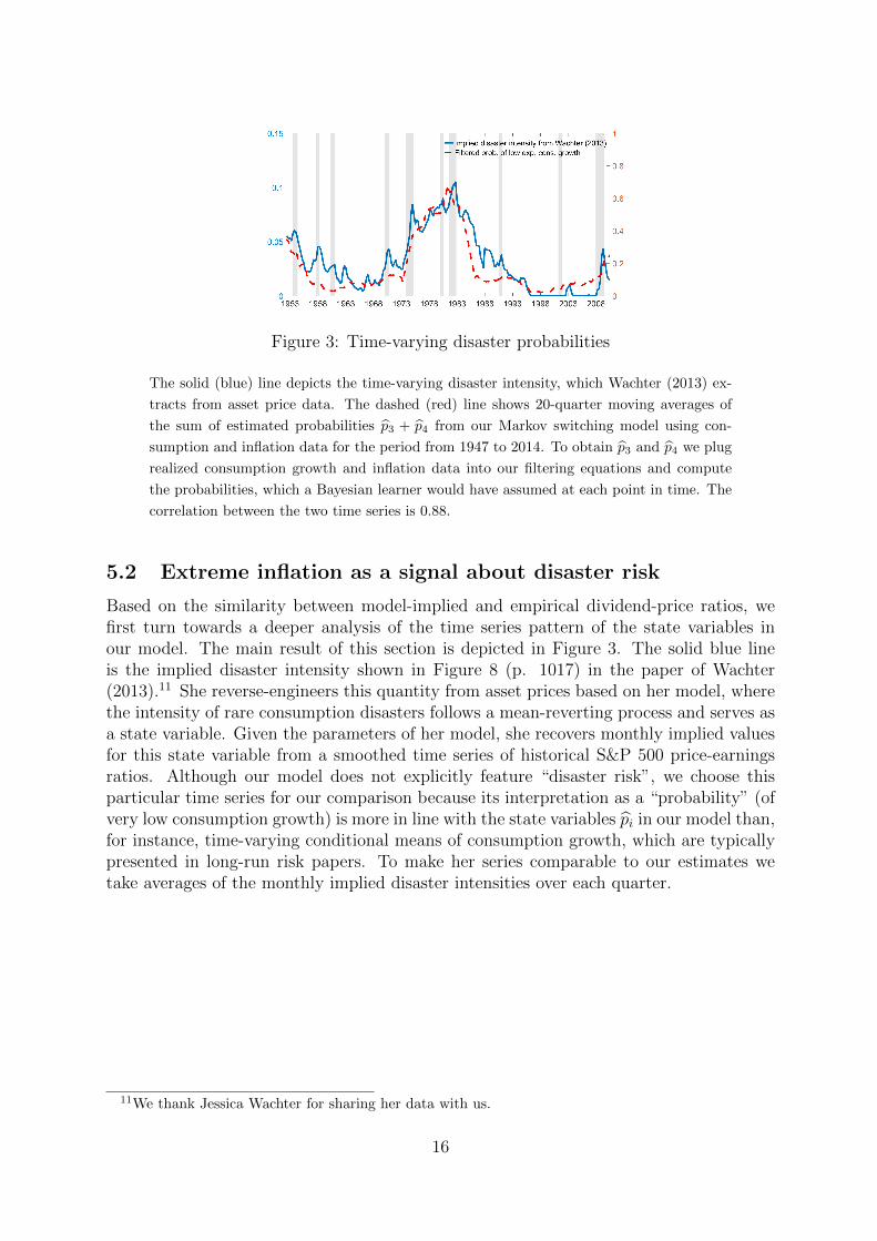
Figure 3: Time-varying disaster probabilities

The solid (blue) line depicts the time-varying disaster intensity, which Wachter (2013) ex-

tracts from asset price data. The dashed (red) line shows 20-quarter moving averages of

the sum of estimated probabilities p3 + p4 from our Markov switching model using con-

sumption and inflation data for the period from 1947 to 2014. To obtain p3 and p4 we plug

realized consumption growth and inflation data into our filtering equations and compute

the probabilities, which a Bayesian learner would have assumed at each point in time. The

correlation between the two time series is 0.88.

5.2 Extreme inflation as a signal about disaster risk

Based on the similarity between model-implied and empirical dividend-price ratios, wefirst turn towards a deeper analysis of the time series pattern of the state variables inour model. The main result of this section is depicted in Figure 3. The solid blue lineis the implied disaster intensity shown in Figure 8 (p. 1017) in the paper of Wachter(2013).11 She reverse-engineers this quantity from asset prices based on her model, wherethe intensity of rare consumption disasters follows a mean-reverting process and serves asa state variable. Given the parameters of her model, she recovers monthly implied valuesfor this state variable from a smoothed time series of historical S&P 500 price-earningsratios. Although our model does not explicitly feature “disaster risk”, we choose thisparticular time series for our comparison because its interpretation as a “probability” (ofvery low consumption growth) is more in line with the state variables pi in our model than,for instance, time-varying conditional means of consumption growth, which are typicallypresented in long-run risk papers. To make her series comparable to our estimates wetake averages of the monthly implied disaster intensities over each quarter.

11We thank Jessica Wachter for sharing her data with us.

16

Figure 4: Disaster probabilities estimated from consumption growth only

The solid (blue) line depicts the time-varying disaster intensity, which Wachter (2013) ex-

tracts from asset price data. The dashed (red) line shows 20-quarter moving averages of the

estimated probability for the state with low expected consumption growth from a Markov

switching model using only consumption data for the period from 1947 to 2014. To obtain

this probability we plug realized consumption growth into our filtering equations and com-

pute the probabilities, which a Bayesian learner would have assumed at each point in time.

The correlation between the two time series is 0.33.

The dashed red line is the sum of the filtered probabilities p3 + p4 from our model.To obtain these estimates we plug realized consumption growth and inflation data intoour filtering equations and compute the probabilities, which a Bayesian learner wouldhave assumed at each point in time. The plot shows 5-year moving averages of theseprobabilities.12

The two series have a correlation of 0.88 over our sample period covering almost 70years. This is particularly remarkable, given that they are computed from very differentdata and using rather different approaches. Furthermore, they share all important trends,peaks, and troughs. There is a pronounced downturn during the 1950s, followed by ratherlow values in the 1960s, a sharp increase during the 1970s up to around 1982, and then,basically following the same kind of cycle, we observe the sharp decline and low levelduring the Great Moderation, followed by the recent spike at the beginning of the GreatRecession. In particular, both the high inflation regime and the deflation regime and theirrespective probabilities are relevant. For instance, a look at the time series plots of thefiltered probabilities in Figure 1 shows that the peak of the two series in the early 1980’scan be traced back to the high probability of the high inflation regime (state 3) over thatperiod, and the deflation regime prevails towards both the beginning and the end of thesample period. This result strongly supports the notion that inflation can serve as a signalfor expected real consumption growth in that it allows to quantify the probability of largenegative future consumption shocks.

To check whether it is indeed inflation that is important here, and not just certainspecial characteristics of the consumption time series, we redo the analysis based on

12We use moving averages in order to account for the smoothing in Wachter (2013). More precisely,for her reverse engineering exercise, she uses the ratio of prices to the previous 10 years of earnings. Thetwo time series depicted in Figure 3 both have an autocorrelation of 0.99.

17

only consumption data, i.e. the univariate baseline model presented in the beginning.Figure 4 presents the time series of the estimated probability for the state with lowexpected growth. Already from a first rough inspection it becomes clear that the disasterintensity is matched much less precisely than before. The correlation between the seriesbased on Wachter (2013) and the filtered probability of being in a bad state derived fromthe consumption-only series goes down to roughly 0.33, but more importantly, the timesseries of estimated probabilities for low consumption growth is substantially off duringbasically all periods when the risk of the economy being in a bad state is actually high,e.g., during most of the 1970’s and 1980’s and also to a certain degree towards the end ofthe sample period. These findings are a clear indication that information about inflationin necessary to obtain reliable estimates for the probability of low real growth.

5.3 Conditional stock return volatilities

Given that Wachter (2013) documents the important role of time-varying disaster inten-sities for the dynamics of second moments of returns, we continue the discussion of ourasset pricing results by analyzing second moments.

We proceed in the following way. We take the time series of filtered probabilities asshown in Figure 1, plug them into our model solution and compute model-implied realprices for equity and for nominal bonds with five years to maturity. From these timeseries of real prices we compute model-implied quarterly real log returns for these twoassets. More precisely, with St and Bt(20) denoting the price of the equity claim and the20-quarter (five-year) nominal zero coupon bond in quarter t, the returns from quarter t toquarter t+1 are computed as ln(St+1 +Dt+1)− lnSt and lnBt+1(19)− lnBt(20). We thenadd log realized inflation to the real returns to obtain nominal returns. The correspondingquantities in the data are quarterly returns of the CRSP value-weighted index and logbond returns computed from the US Treasury yield curve data provided by Gurkaynak,Sack, and Wright (2007)13 from 1962 on. As the final input to our analyses we compute20-quarter rolling window return volatilities and correlations and regress them on (thelogarithm of) 20-quarter moving averages of the relevant state probabilities p. Note thatthese right-hand variables are the same for model and data in all the regressions reportedbelow.

For the regressions in the model and in the data we state Newey-West adjusted t-statistics with 20 lags, but in addition we also provide confidence intervals derived froma Monte Carlo simulation of the model (shown in square brackets below the respectivecoefficient). Here we first simulate the model given the dynamics for the fundamentals andthe filtered probabilities in Equations (1) to (3) with monthly time increments over a timespan of 68 years, corresponding to the length of our sample period for the macroeconomicvariables. These monthly data are then aggregated to quarterly and used in the regressionsin the same way as described before, i.e., we only use the later 50 years of each samplepath, corresponding to the period over which financial market data are available. Werepeat this exercise 5,000 times to obtain the 90% confidence intervals.14

13The data are available for download at http://www.federalreserve.gov/pubs/feds/2006/

200628/200628abs.html.14Due to the discretization error in the simulation it sometimes happens that the sum of the filtered

probabilities exceeds 1 by a very small amount. In that case we rescale the filtered probabilities such

18

Data Model

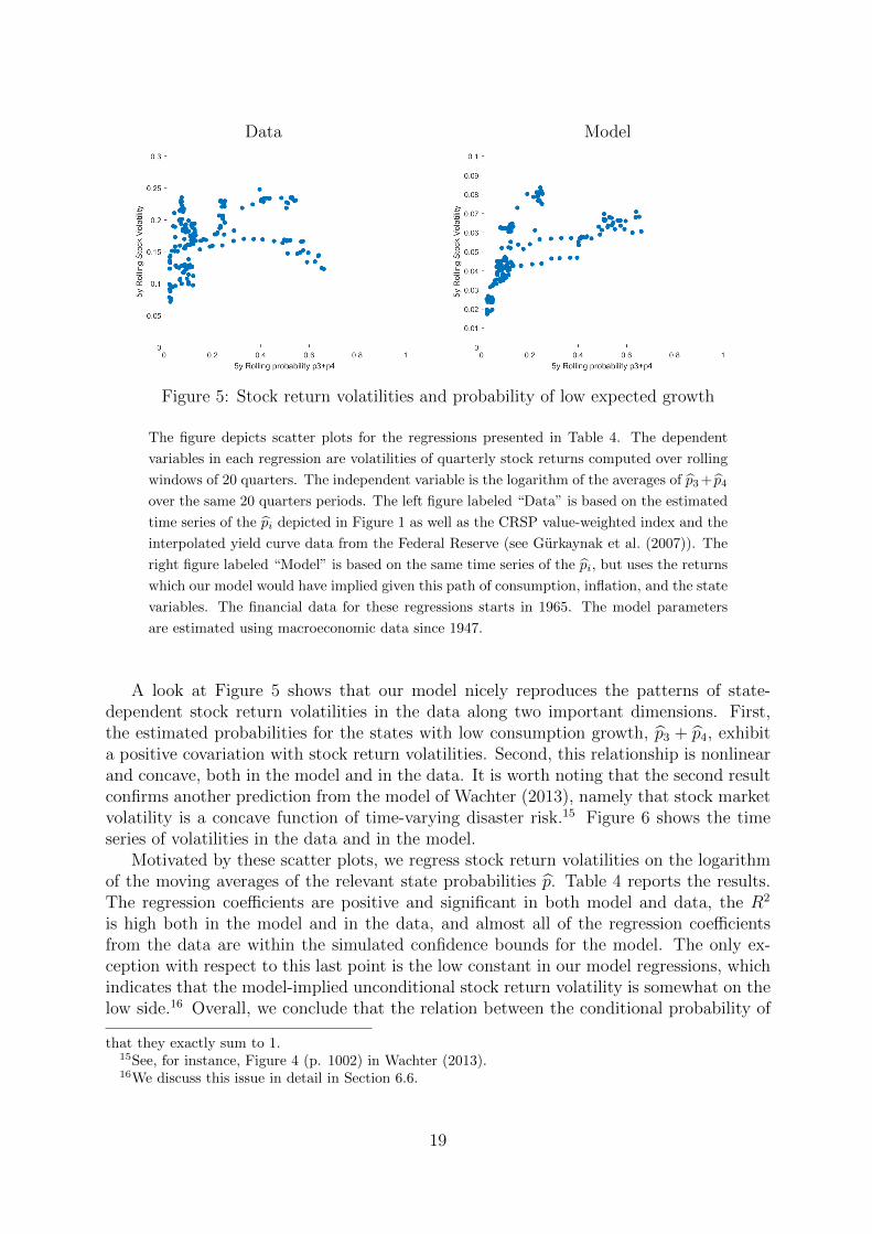
Figure 5: Stock return volatilities and probability of low expected growth

The figure depicts scatter plots for the regressions presented in Table 4. The dependent

variables in each regression are volatilities of quarterly stock returns computed over rolling

windows of 20 quarters. The independent variable is the logarithm of the averages of p3+ p4

over the same 20 quarters periods. The left figure labeled “Data” is based on the estimated

time series of the pi depicted in Figure 1 as well as the CRSP value-weighted index and the

interpolated yield curve data from the Federal Reserve (see Gurkaynak et al. (2007)). The

right figure labeled “Model” is based on the same time series of the pi, but uses the returns

which our model would have implied given this path of consumption, inflation, and the state

variables. The financial data for these regressions starts in 1965. The model parameters

are estimated using macroeconomic data since 1947.

A look at Figure 5 shows that our model nicely reproduces the patterns of state-dependent stock return volatilities in the data along two important dimensions. First,the estimated probabilities for the states with low consumption growth, p3 + p4, exhibita positive covariation with stock return volatilities. Second, this relationship is nonlinearand concave, both in the model and in the data. It is worth noting that the second resultconfirms another prediction from the model of Wachter (2013), namely that stock marketvolatility is a concave function of time-varying disaster risk.15 Figure 6 shows the timeseries of volatilities in the data and in the model.

Motivated by these scatter plots, we regress stock return volatilities on the logarithmof the moving averages of the relevant state probabilities p. Table 4 reports the results.The regression coefficients are positive and significant in both model and data, the R2

is high both in the model and in the data, and almost all of the regression coefficientsfrom the data are within the simulated confidence bounds for the model. The only ex-ception with respect to this last point is the low constant in our model regressions, whichindicates that the model-implied unconditional stock return volatility is somewhat on thelow side.16 Overall, we conclude that the relation between the conditional probability of

that they exactly sum to 1.15See, for instance, Figure 4 (p. 1002) in Wachter (2013).16We discuss this issue in detail in Section 6.6.

19

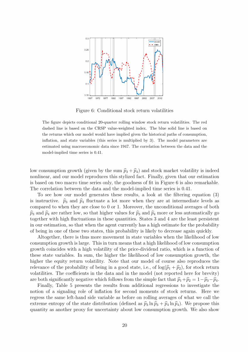
Figure 6: Conditional stock return volatilities

The figure depicts conditional 20-quarter rolling window stock return volatilities. The red

dashed line is based on the CRSP value-weighted index. The blue solid line is based on

the returns which our model would have implied given the historical paths of consumption,

inflation, and state variables (this series is multiplied by 3). The model parameters are

estimated using macroeconomic data since 1947. The correlation between the data and the

model-implied time series is 0.41.

low consumption growth (given by the sum p3 + p4) and stock market volatility is indeednonlinear, and our model reproduces this stylized fact. Finally, given that our estimationis based on two macro time series only, the goodness of fit in Figure 6 is also remarkable.The correlation between the data and the model-implied time series is 0.41.

To see how our model generates these results, a look at the filtering equation (3)is instructive. p3 and p4 fluctuate a lot more when they are at intermediate levels ascompared to when they are close to 0 or 1. Moreover, the unconditional averages of bothp3 and p4 are rather low, so that higher values for p3 and p4 more or less automatically gotogether with high fluctuations in these quantities. States 3 and 4 are the least persistentin our estimation, so that when the agent currently has a high estimate for the probabilityof being in one of these two states, this probability is likely to decrease again quickly.

Altogether, there is thus more movement in state variables when the likelihood of lowconsumption growth is large. This in turn means that a high likelihood of low consumptiongrowth coincides with a high volatility of the price-dividend ratio, which is a function ofthese state variables. In sum, the higher the likelihood of low consumption growth, thehigher the equity return volatility. Note that our model of course also reproduces therelevance of the probability of being in a good state, i.e., of log(p1 + p2), for stock returnvolatilities. The coefficients in the data and in the model (not reported here for brevity)are both significantly negative which follows from the simple fact that p1+p2 = 1−p3−p4.

Finally, Table 5 presents the results from additional regressions to investigate thenotion of a signaling role of inflation for second moments of stock returns. Here weregress the same left-hand side variable as before on rolling averages of what we call theextreme entropy of the state distribution (defined as p3 ln p3 + p4 ln p4). We propose thisquantity as another proxy for uncertainty about low consumption growth. We also show

20

Panel A: Modelconst. log(p3) log(p4) log(p3 + p4) Adj. R2

0.114 0.009 0.012 0.733(12.627) (10.833) (4.724)

[0.085, 0.174] [0.004, 0.020] [0.000, 0.023] [0.220, 0.785]

0.079 0.015 0.615(12.143) (5.997)

[0.071, 0.129] [0.007, 0.029] [0.104, 0.763]

Panel B: Dataconst. log(p3) log(p4) log(p3 + p4) Adj. R2

0.278 0.012 0.023 0.304(12.679) (1.416) (4.475)

0.214 0.022 0.214(9.056) (1.976)

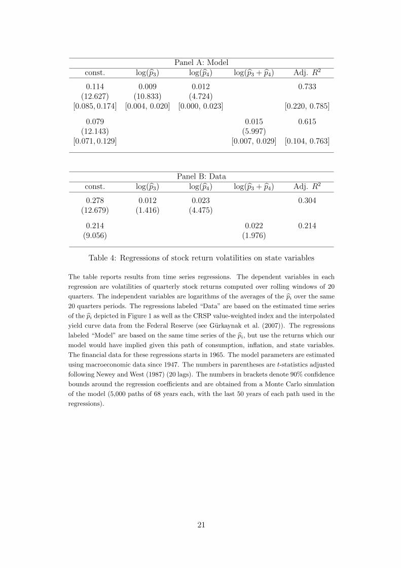
Table 4: Regressions of stock return volatilities on state variables

The table reports results from time series regressions. The dependent variables in each

regression are volatilities of quarterly stock returns computed over rolling windows of 20

quarters. The independent variables are logarithms of the averages of the pi over the same

20 quarters periods. The regressions labeled “Data” are based on the estimated time series

of the pi depicted in Figure 1 as well as the CRSP value-weighted index and the interpolated

yield curve data from the Federal Reserve (see Gurkaynak et al. (2007)). The regressions

labeled “Model” are based on the same time series of the pi, but use the returns which our

model would have implied given this path of consumption, inflation, and state variables.

The financial data for these regressions starts in 1965. The model parameters are estimated

using macroeconomic data since 1947. The numbers in parentheses are t-statistics adjusted

following Newey and West (1987) (20 lags). The numbers in brackets denote 90% confidence

bounds around the regression coefficients and are obtained from a Monte Carlo simulation

of the model (5,000 paths of 68 years each, with the last 50 years of each path used in the

regressions).

21

Panel A: Modelconst. extreme entropy expected inflation realized inflation Adj. R2

0.001 0.269 0.538(0.106) (5.859)

[−0.038, 0.053] [0.041, 0.618] [0.002, 0.609]0.032 0.004 0.159

(2.504) (1.930)[0.009, 0.064] [-0.001, 0.015] [-0.007, 0.584]

0.036 0.003 0.147(3.130) (1.801)

[0.018, 0.063] [-0.001, 0.012] [-0.007, 0.578]Panel B: Data

const. extreme entropy expected inflation realized inflation Adj. R2

0.097 0.399 0.187(2.607) (2.320)0.147 0.006 0.036

(4.814) (0.855)0.153 0.004 0.040

(6.010) (0.781)

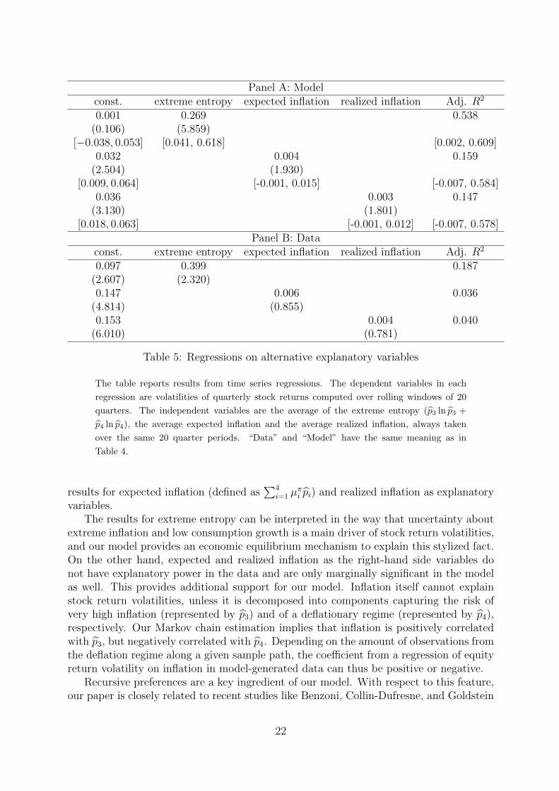
Table 5: Regressions on alternative explanatory variables

The table reports results from time series regressions. The dependent variables in each

regression are volatilities of quarterly stock returns computed over rolling windows of 20

quarters. The independent variables are the average of the extreme entropy (p3 ln p3 +

p4 ln p4), the average expected inflation and the average realized inflation, always taken

over the same 20 quarter periods. “Data” and “Model” have the same meaning as in

Table 4.

results for expected inflation (defined as∑4

i=1 µπi pi) and realized inflation as explanatory

variables.The results for extreme entropy can be interpreted in the way that uncertainty about

extreme inflation and low consumption growth is a main driver of stock return volatilities,and our model provides an economic equilibrium mechanism to explain this stylized fact.On the other hand, expected and realized inflation as the right-hand side variables donot have explanatory power in the data and are only marginally significant in the modelas well. This provides additional support for our model. Inflation itself cannot explainstock return volatilities, unless it is decomposed into components capturing the risk ofvery high inflation (represented by p3) and of a deflationary regime (represented by p4),respectively. Our Markov chain estimation implies that inflation is positively correlatedwith p3, but negatively correlated with p4. Depending on the amount of observations fromthe deflation regime along a given sample path, the coefficient from a regression of equityreturn volatility on inflation in model-generated data can thus be positive or negative.

Recursive preferences are a key ingredient of our model. With respect to this feature,our paper is closely related to recent studies like Benzoni, Collin-Dufresne, and Goldstein

22

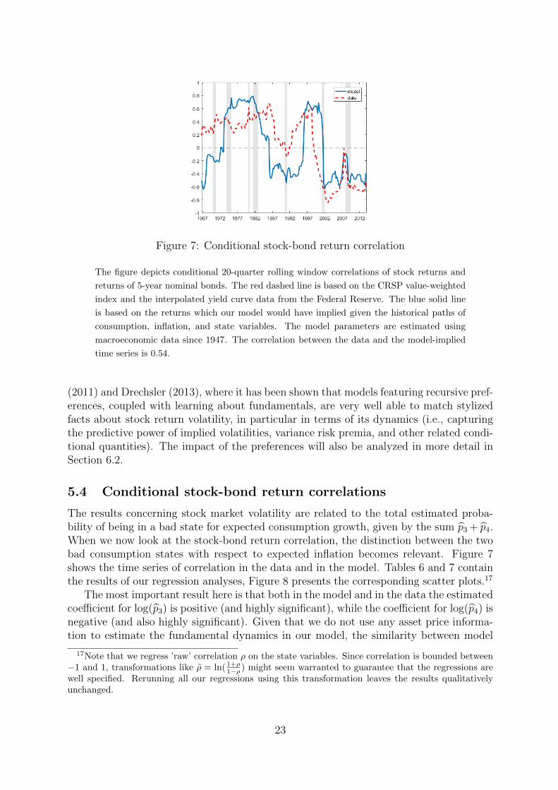
Figure 7: Conditional stock-bond return correlation

The figure depicts conditional 20-quarter rolling window correlations of stock returns and

returns of 5-year nominal bonds. The red dashed line is based on the CRSP value-weighted

index and the interpolated yield curve data from the Federal Reserve. The blue solid line

is based on the returns which our model would have implied given the historical paths of

consumption, inflation, and state variables. The model parameters are estimated using

macroeconomic data since 1947. The correlation between the data and the model-implied

time series is 0.54.

(2011) and Drechsler (2013), where it has been shown that models featuring recursive pref-erences, coupled with learning about fundamentals, are very well able to match stylizedfacts about stock return volatility, in particular in terms of its dynamics (i.e., capturingthe predictive power of implied volatilities, variance risk premia, and other related condi-tional quantities). The impact of the preferences will also be analyzed in more detail inSection 6.2.

5.4 Conditional stock-bond return correlations

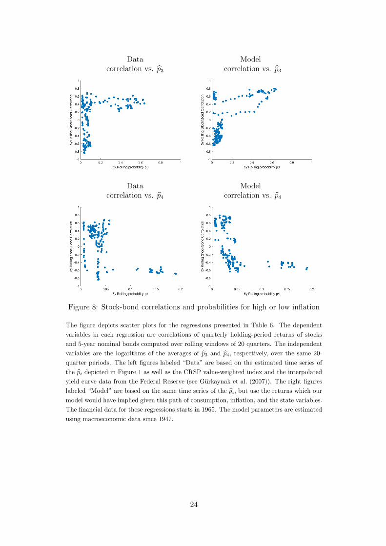
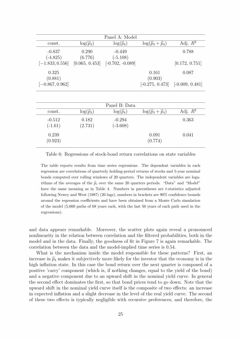
The results concerning stock market volatility are related to the total estimated proba-bility of being in a bad state for expected consumption growth, given by the sum p3 + p4.When we now look at the stock-bond return correlation, the distinction between the twobad consumption states with respect to expected inflation becomes relevant. Figure 7shows the time series of correlation in the data and in the model. Tables 6 and 7 containthe results of our regression analyses, Figure 8 presents the corresponding scatter plots.17

The most important result here is that both in the model and in the data the estimatedcoefficient for log(p3) is positive (and highly significant), while the coefficient for log(p4) isnegative (and also highly significant). Given that we do not use any asset price informa-tion to estimate the fundamental dynamics in our model, the similarity between model

17Note that we regress ’raw’ correlation ρ on the state variables. Since correlation is bounded between−1 and 1, transformations like ρ = ln( 1+ρ

1−ρ ) might seem warranted to guarantee that the regressions arewell specified. Rerunning all our regressions using this transformation leaves the results qualitativelyunchanged.

23

Data Modelcorrelation vs. p3 correlation vs. p3

Data Modelcorrelation vs. p4 correlation vs. p4

Figure 8: Stock-bond correlations and probabilities for high or low inflation

The figure depicts scatter plots for the regressions presented in Table 6. The dependent

variables in each regression are correlations of quarterly holding-period returns of stocks

and 5-year nominal bonds computed over rolling windows of 20 quarters. The independent

variables are the logarithms of the averages of p3 and p4, respectively, over the same 20-

quarter periods. The left figures labeled “Data” are based on the estimated time series of

the pi depicted in Figure 1 as well as the CRSP value-weighted index and the interpolated

yield curve data from the Federal Reserve (see Gurkaynak et al. (2007)). The right figures

labeled “Model” are based on the same time series of the pi, but use the returns which our

model would have implied given this path of consumption, inflation, and the state variables.

The financial data for these regressions starts in 1965. The model parameters are estimated

using macroeconomic data since 1947.

24

Panel A: Modelconst. log(p3) log(p4) log(p3 + p4) Adj. R2

-0.837 0.290 -0.449 0.788(-4.825) (6.776) (-5.108)

[−1.833, 0.556] [0.065, 0.453] [-0.702, -0.089] [0.172, 0.751]

0.325 0.161 0.087(0.881) (0.903)

[−0.867, 0.962] [-0.275, 0.473] [-0.009, 0.481]

Panel B: Dataconst. log(p3) log(p4) log(p3 + p4) Adj. R2

-0.512 0.182 -0.294 0.363(-1.61) (2.731) (-3.608)

0.239 0.091 0.041(0.923) (0.774)

Table 6: Regressions of stock-bond return correlations on state variables

The table reports results from time series regressions. The dependent variables in each

regression are correlations of quarterly holding-period returns of stocks and 5-year nominal

bonds computed over rolling windows of 20 quarters. The independent variables are loga-

rithms of the averages of the pi over the same 20 quarters periods. “Data” and “Model”

have the same meaning as in Table 4. Numbers in parentheses are t-statistics adjusted

following Newey and West (1987) (20 lags), numbers in brackets are 90% confidence bounds

around the regression coefficients and have been obtained from a Monte Carlo simulation

of the model (5,000 paths of 68 years each, with the last 50 years of each path used in the

regressions).

and data appears remarkable. Moreover, the scatter plots again reveal a pronouncednonlinearity in the relation between correlation and the filtered probabilities, both in themodel and in the data. Finally, the goodness of fit in Figure 7 is again remarkable. Thecorrelation between the data and the model-implied time series is 0.54.

What is the mechanism inside the model responsible for these patterns? First, anincrease in p3 makes it subjectively more likely for the investor that the economy is in thehigh inflation state. In this case the bond return over the next quarter is composed of apositive ’carry’ component (which is, if nothing changes, equal to the yield of the bond)and a negative component due to an upward shift in the nominal yield curve. In generalthe second effect dominates the first, so that bond prices tend to go down. Note that theupward shift in the nominal yield curve itself is the composite of two effects: an increasein expected inflation and a slight decrease in the level of the real yield curve. The secondof these two effects is typically negligible with recursive preferences, and therefore, the

25

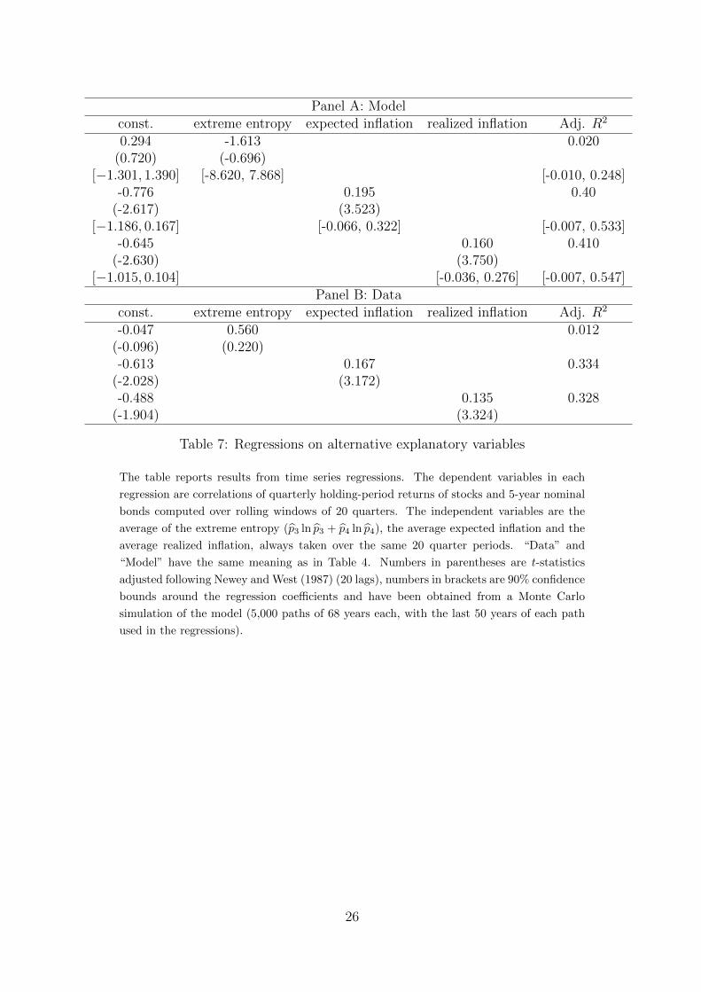
Panel A: Modelconst. extreme entropy expected inflation realized inflation Adj. R2

0.294 -1.613 0.020(0.720) (-0.696)

[−1.301, 1.390] [-8.620, 7.868] [-0.010, 0.248]-0.776 0.195 0.40

(-2.617) (3.523)[−1.186, 0.167] [-0.066, 0.322] [-0.007, 0.533]

-0.645 0.160 0.410(-2.630) (3.750)

[−1.015, 0.104] [-0.036, 0.276] [-0.007, 0.547]Panel B: Data

const. extreme entropy expected inflation realized inflation Adj. R2

-0.047 0.560 0.012(-0.096) (0.220)-0.613 0.167 0.334

(-2.028) (3.172)-0.488 0.135 0.328

(-1.904) (3.324)

Table 7: Regressions on alternative explanatory variables

The table reports results from time series regressions. The dependent variables in each

regression are correlations of quarterly holding-period returns of stocks and 5-year nominal

bonds computed over rolling windows of 20 quarters. The independent variables are the

average of the extreme entropy (p3 ln p3 + p4 ln p4), the average expected inflation and the

average realized inflation, always taken over the same 20 quarter periods. “Data” and

“Model” have the same meaning as in Table 4. Numbers in parentheses are t-statistics

adjusted following Newey and West (1987) (20 lags), numbers in brackets are 90% confidence

bounds around the regression coefficients and have been obtained from a Monte Carlo

simulation of the model (5,000 paths of 68 years each, with the last 50 years of each path

used in the regressions).

26

nominal yield curve shifts upwards in response to an increase in p3. The stock returnupon a positive shock to p3 depends on real quantities only. A high p3 implies that theeconomy is more likely to be in a low consumption growth regime, and stock prices tendto be low in such an environment. Taken together, the reactions of bond and stock pricesto an increase in p3 go in the same direction, implying a positive correlation.

State 4 is a low inflation state with low growth, so the response of bond prices to ahigh p4 is different. Again, there is the positive carry return. But now there is also anadditional positive return because the nominal yield curve shifts downwards in responseto a higher probability for deflation. When deflation becomes more likely, the level ofthe nominal yield curve must decrease. Altogether, the impact of a high probability p4on bond returns is large and positive. At the same time, such a high p4 signals a highlikelihood of low (even negative) expected consumption growth, which depresses equityprices. In sum, the impact of a high likelihood for the deflationary regime is strong onboth stock and bond prices, but it is of opposite signs, implying a negative correlationbetween the two types of assets.

The above findings concerning the role of p3 and p4 for the conditional stock-bondcorrelation are well in line with the literature. In a purely empirical paper, Baele et al.(2010) try to fit the correlations of daily stock and bond returns with a multi-factormodel. They find that macro factors (in particular output gap and inflation) do not addmuch explanatory power when the loadings of stock and bond returns are assumed tobe constant over time. But the performance of the macro factors improves in a regimeswitching estimation when the loadings are allowed to switch sign. Our findings arepotentially related to theirs in the sense that we show that the overall risk of low expectedconsumption growth, proxied by the sum p3 + p4, does not predict correlation, neither inthe model nor in the data. The coefficients on realized and expected inflation are positive,but the simulated confidence bounds always include zero.

For both model and data, the regressions with extreme entropy generate the expectedresult with insignificant coefficient estimates. The reason is again that this measurecaptures general uncertainty about bad consumption growth states. Uncertainty aboutbeing in the deflation state, however, decreases correlation, whereas uncertainty aboutthe high inflation state increases it. An aggregate measure of uncertainty cannot capturethese two opposing effects adequately.

6 Robustness

6.1 Overview

In the previous sections, we have shown that long-run risk and time-varying disaster riskcan be linked to time variation in the stock-bond return correlation if one accounts for thesignaling role of inflation. Since these results have been obtained within the frameworkof a particular asset pricing model, we are going to discuss why the major modelingassumptions are necessary to obtain this result and how our findings would change insimplified versions of our model. Finally, we will also present evidence from additionaldata samples to verify that our findings are not due to a specific choice of these samples.

27

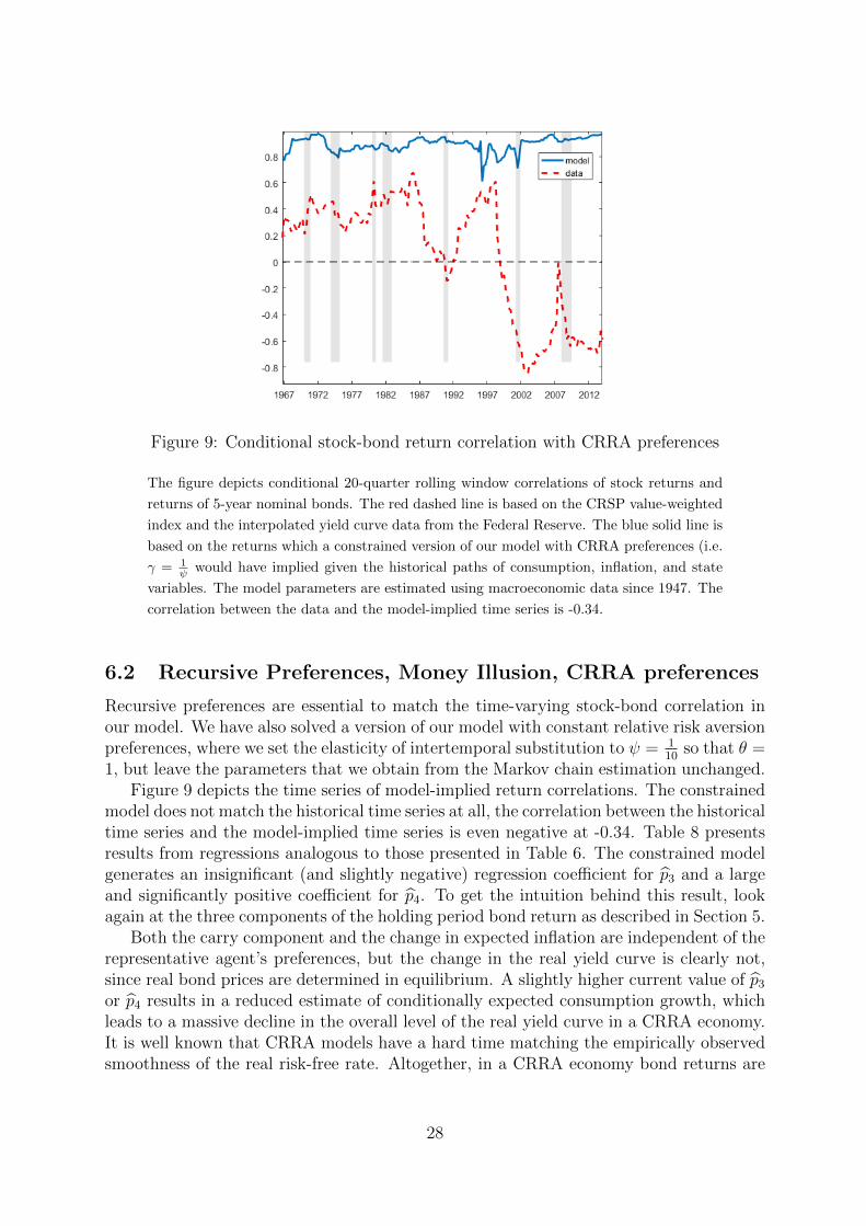
Figure 9: Conditional stock-bond return correlation with CRRA preferences

The figure depicts conditional 20-quarter rolling window correlations of stock returns and

returns of 5-year nominal bonds. The red dashed line is based on the CRSP value-weighted

index and the interpolated yield curve data from the Federal Reserve. The blue solid line is

based on the returns which a constrained version of our model with CRRA preferences (i.e.

γ = 1ψ would have implied given the historical paths of consumption, inflation, and state

variables. The model parameters are estimated using macroeconomic data since 1947. The

correlation between the data and the model-implied time series is -0.34.

6.2 Recursive Preferences, Money Illusion, CRRA preferences

Recursive preferences are essential to match the time-varying stock-bond correlation inour model. We have also solved a version of our model with constant relative risk aversionpreferences, where we set the elasticity of intertemporal substitution to ψ = 1

10so that θ =

1, but leave the parameters that we obtain from the Markov chain estimation unchanged.Figure 9 depicts the time series of model-implied return correlations. The constrained

model does not match the historical time series at all, the correlation between the historicaltime series and the model-implied time series is even negative at -0.34. Table 8 presentsresults from regressions analogous to those presented in Table 6. The constrained modelgenerates an insignificant (and slightly negative) regression coefficient for p3 and a largeand significantly positive coefficient for p4. To get the intuition behind this result, lookagain at the three components of the holding period bond return as described in Section 5.

Both the carry component and the change in expected inflation are independent of therepresentative agent’s preferences, but the change in the real yield curve is clearly not,since real bond prices are determined in equilibrium. A slightly higher current value of p3or p4 results in a reduced estimate of conditionally expected consumption growth, whichleads to a massive decline in the overall level of the real yield curve in a CRRA economy.It is well known that CRRA models have a hard time matching the empirically observedsmoothness of the real risk-free rate. Altogether, in a CRRA economy bond returns are

28

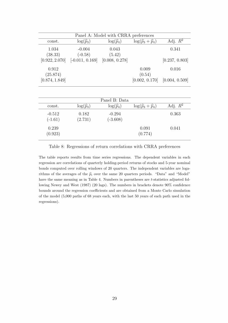
Panel A: Model with CRRA preferencesconst. log(p3) log(p4) log(p3 + p4) Adj. R2

1.034 -0.004 0.043 0.341(38.33) (-0.58) (5.42)

[0.922, 2.070] [-0.011, 0.169] [0.008, 0.278] [0.237, 0.803]

0.912 0.009 0.016(25.874) (0.54)

[0.874, 1.849] [0.002, 0.170] [0.004, 0.509]

Panel B: Dataconst. log(p3) log(p4) log(p3 + p4) Adj. R2

-0.512 0.182 -0.294 0.363(-1.61) (2.731) (-3.608)

0.239 0.091 0.041(0.923) (0.774)

Table 8: Regressions of return correlations with CRRA preferences

The table reports results from time series regressions. The dependent variables in each

regression are correlations of quarterly holding-period returns of stocks and 5-year nominal

bonds computed over rolling windows of 20 quarters. The independent variables are loga-

rithms of the averages of the pi over the same 20 quarters periods. “Data” and “Model”

have the same meaning as in Table 4. Numbers in parentheses are t-statistics adjusted fol-

lowing Newey and West (1987) (20 lags). The numbers in brackets denote 90% confidence

bounds around the regression coefficients and are obtained from a Monte Carlo simulation

of the model (5,000 paths of 68 years each, with the last 50 years of each path used in the

regressions).

29

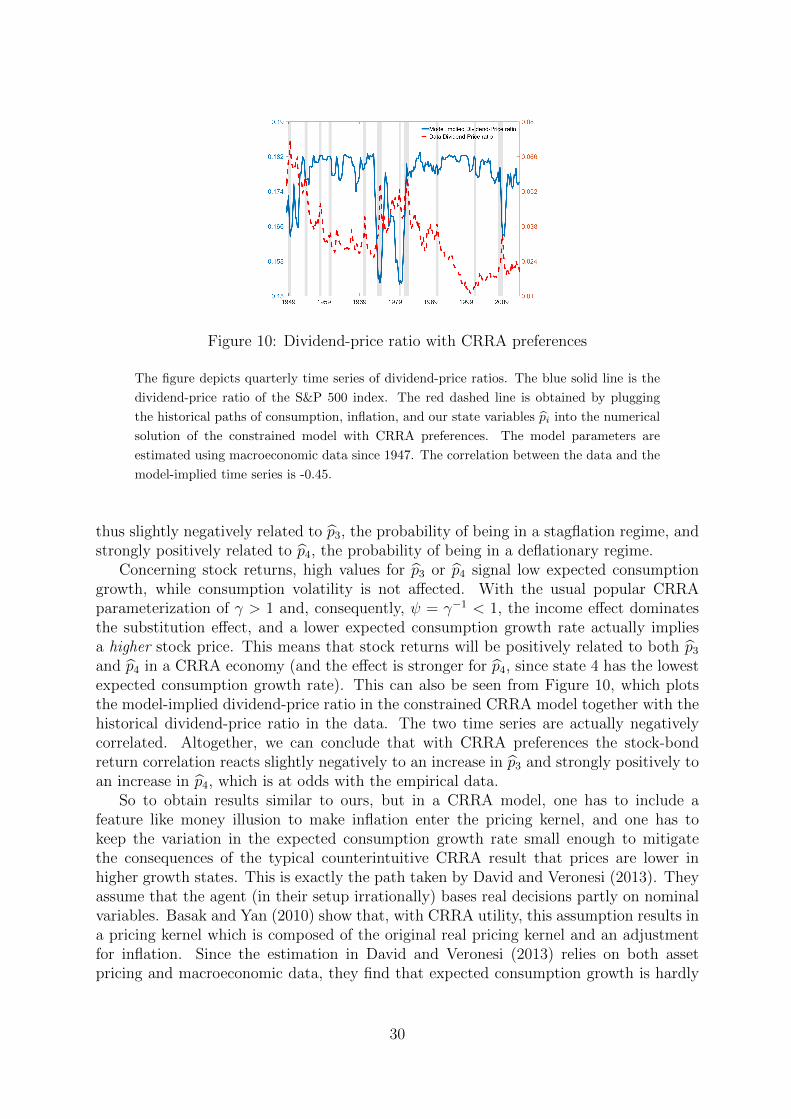
Figure 10: Dividend-price ratio with CRRA preferences

The figure depicts quarterly time series of dividend-price ratios. The blue solid line is the

dividend-price ratio of the S&P 500 index. The red dashed line is obtained by plugging

the historical paths of consumption, inflation, and our state variables pi into the numerical

solution of the constrained model with CRRA preferences. The model parameters are

estimated using macroeconomic data since 1947. The correlation between the data and the

model-implied time series is -0.45.

thus slightly negatively related to p3, the probability of being in a stagflation regime, andstrongly positively related to p4, the probability of being in a deflationary regime.

Concerning stock returns, high values for p3 or p4 signal low expected consumptiongrowth, while consumption volatility is not affected. With the usual popular CRRAparameterization of γ > 1 and, consequently, ψ = γ−1 < 1, the income effect dominatesthe substitution effect, and a lower expected consumption growth rate actually impliesa higher stock price. This means that stock returns will be positively related to both p3and p4 in a CRRA economy (and the effect is stronger for p4, since state 4 has the lowestexpected consumption growth rate). This can also be seen from Figure 10, which plotsthe model-implied dividend-price ratio in the constrained CRRA model together with thehistorical dividend-price ratio in the data. The two time series are actually negativelycorrelated. Altogether, we can conclude that with CRRA preferences the stock-bondreturn correlation reacts slightly negatively to an increase in p3 and strongly positively toan increase in p4, which is at odds with the empirical data.

So to obtain results similar to ours, but in a CRRA model, one has to include afeature like money illusion to make inflation enter the pricing kernel, and one has tokeep the variation in the expected consumption growth rate small enough to mitigatethe consequences of the typical counterintuitive CRRA result that prices are lower inhigher growth states. This is exactly the path taken by David and Veronesi (2013). Theyassume that the agent (in their setup irrationally) bases real decisions partly on nominalvariables. Basak and Yan (2010) show that, with CRRA utility, this assumption results ina pricing kernel which is composed of the original real pricing kernel and an adjustmentfor inflation. Since the estimation in David and Veronesi (2013) relies on both assetpricing and macroeconomic data, they find that expected consumption growth is hardly

30

varying across states, so they constrain it to be equal across states in their followingnumerical evaluation (p. 703). This clearly contradicts our estimation results presentedabove. Relying on recursive utility, we do not have to restrict the fundamental dynamicsin such a way, and we also do not need to assume any sort of bounded rationality on thepart of the representative investor.

6.3 Full Information

In our model we make the assumption that the current state of the economy is unobserv-able and has to be filtered from macro data. To see why this assumption is necessary, wehave also solved a version of our model with full information. The theoretical solution ispresented in Appendix D, the proof is a slight modification of the proof in Appendix A ofBranger et al. (2016). In an economy with four states, we obtain four possible values forthe wealth-consumption ratio, for the price-dividend ratio and for the price of a nominalbond with a given maturity.

To evaluate the model with full information, we perform the following exercise, which issimilar to the exercise in Section 5. Our Markov chain estimation above gives time seriesof ex-post probabilities that the economy was in one of the four states at a particularhistorical point in time. We round these probabilities (which are already close to 0 or 1)to exactly 0 or 1, respectively, so that we get a “clean” historical time series of economicstates. Combining this time series with the model solution gives us historical time series ofwealth-consumption ratios, price-dividend ratios and bond prices under the assumption offull information. From these time series and historical consumption and inflation shocks,we then again compute time series of model-implied returns, and from these model-impliedreturns we compute rolling-window correlations and volatilities as before.

For brevity, we discuss the stock-bond return correlation results only because thefailure of a full information model becomes most evident here. Figure 11 shows therespective time series from model-generated and empirical data. The two time series differsubstantially throughout the sample. Most importantly, the model with full informationhas problems to generate the negative correlation between stock and bond returns thatwe see in the data in the most recent years.

The reason for this failure can be traced back to the estimated Markov chain transitionprobabilities (Table 2). According to the estimation, there is a zero probability to enterthe deflationary state 4 from state 2 or 3. In an economy with full information, this impliesthat the threat of entering the worst possible economic state in the next quarter is shutdown completely for about 70% of the time. In an economy with partial information,on the other hand, there is always a nonzero subjective probability assigned to beingin a state from which the economy can slide into state 4. Consequently, the averagelevel of disaster risk is much lower in the full information economy, and moreover thepricing effect of the fear of deflation, as described in Section 5, is reduced substantially.For instance, in the full information economy the price-dividend ratio of the stock is thelargest in states 2 and 3 (155.5 and 148.1, respectively) and the smallest in states 1 and4 (145.6 and 143.0). Since this fear of deflation is the key mechanism that generatesnegative comovement between stock and bond returns, the full information model cannotreproduce the negative stock-bond return correlation.

31

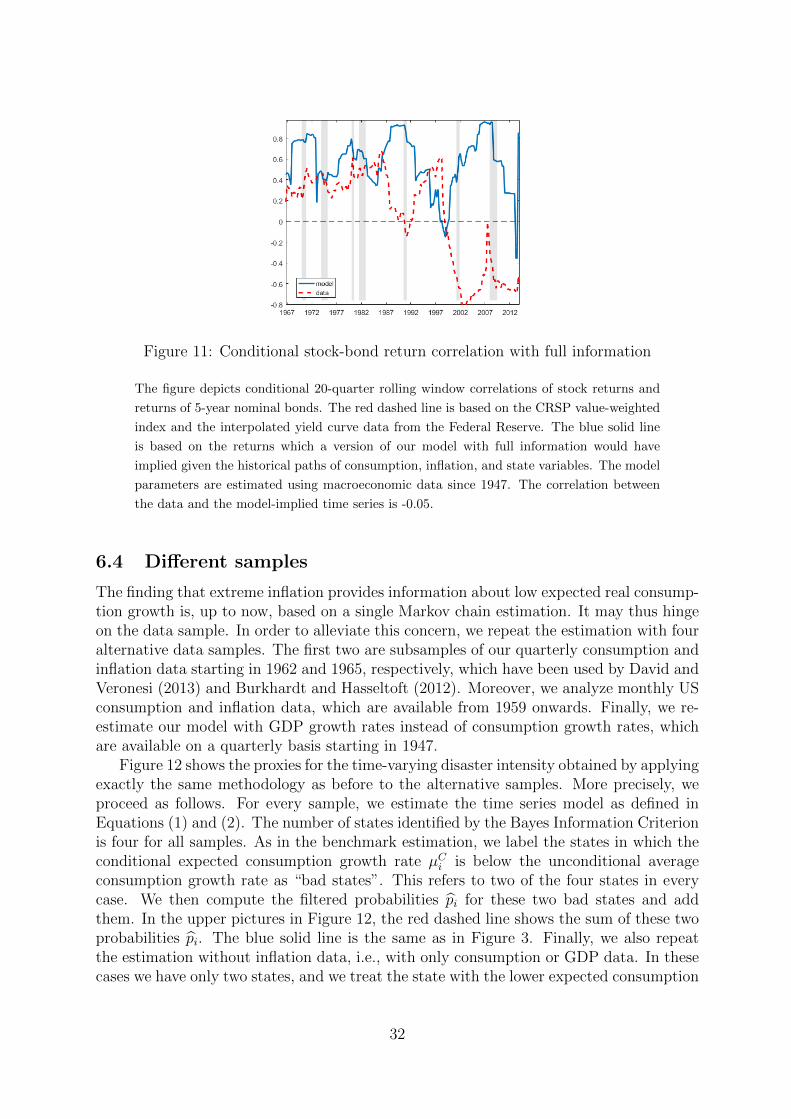
Figure 11: Conditional stock-bond return correlation with full information

The figure depicts conditional 20-quarter rolling window correlations of stock returns and

returns of 5-year nominal bonds. The red dashed line is based on the CRSP value-weighted

index and the interpolated yield curve data from the Federal Reserve. The blue solid line

is based on the returns which a version of our model with full information would have

implied given the historical paths of consumption, inflation, and state variables. The model

parameters are estimated using macroeconomic data since 1947. The correlation between

the data and the model-implied time series is -0.05.

6.4 Different samples

The finding that extreme inflation provides information about low expected real consump-tion growth is, up to now, based on a single Markov chain estimation. It may thus hingeon the data sample. In order to alleviate this concern, we repeat the estimation with fouralternative data samples. The first two are subsamples of our quarterly consumption andinflation data starting in 1962 and 1965, respectively, which have been used by David andVeronesi (2013) and Burkhardt and Hasseltoft (2012). Moreover, we analyze monthly USconsumption and inflation data, which are available from 1959 onwards. Finally, we re-estimate our model with GDP growth rates instead of consumption growth rates, whichare available on a quarterly basis starting in 1947.

Figure 12 shows the proxies for the time-varying disaster intensity obtained by applyingexactly the same methodology as before to the alternative samples. More precisely, weproceed as follows. For every sample, we estimate the time series model as defined inEquations (1) and (2). The number of states identified by the Bayes Information Criterionis four for all samples. As in the benchmark estimation, we label the states in which theconditional expected consumption growth rate µCi is below the unconditional averageconsumption growth rate as “bad states”. This refers to two of the four states in everycase. We then compute the filtered probabilities pi for these two bad states and addthem. In the upper pictures in Figure 12, the red dashed line shows the sum of these twoprobabilities pi. The blue solid line is the same as in Figure 3. Finally, we also repeatthe estimation without inflation data, i.e., with only consumption or GDP data. In thesecases we have only two states, and we treat the state with the lower expected consumption

32

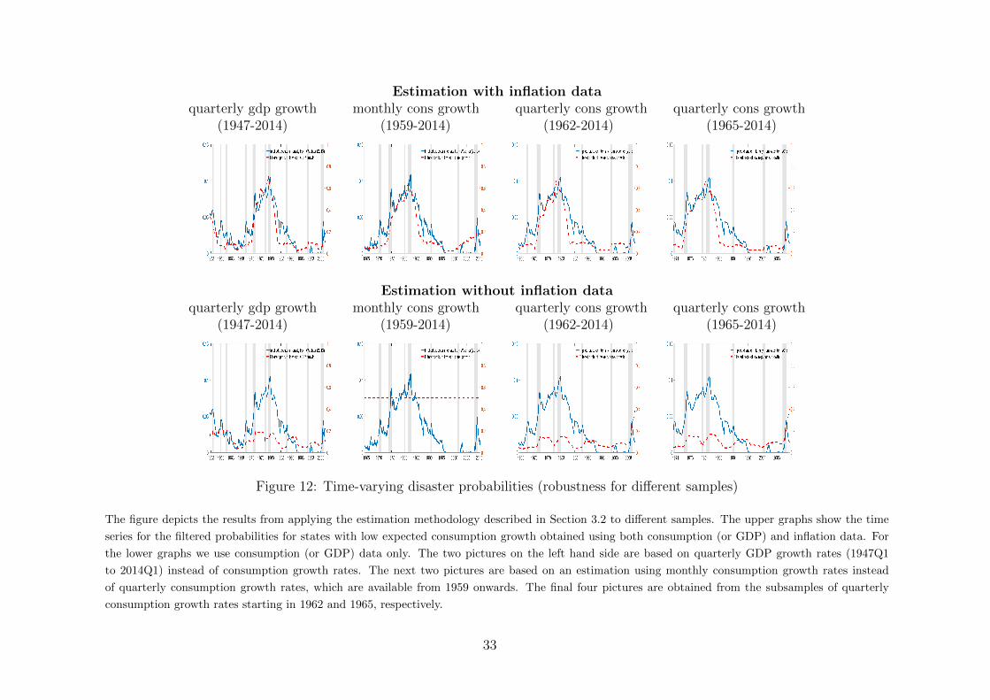
Estimation with inflation dataquarterly gdp growth monthly cons growth quarterly cons growth quarterly cons growth

(1947-2014) (1959-2014) (1962-2014) (1965-2014)

Estimation without inflation dataquarterly gdp growth monthly cons growth quarterly cons growth quarterly cons growth

(1947-2014) (1959-2014) (1962-2014) (1965-2014)

Figure 12: Time-varying disaster probabilities (robustness for different samples)

The figure depicts the results from applying the estimation methodology described in Section 3.2 to different samples. The upper graphs show the time

series for the filtered probabilities for states with low expected consumption growth obtained using both consumption (or GDP) and inflation data. For

the lower graphs we use consumption (or GDP) data only. The two pictures on the left hand side are based on quarterly GDP growth rates (1947Q1

to 2014Q1) instead of consumption growth rates. The next two pictures are based on an estimation using monthly consumption growth rates instead

of quarterly consumption growth rates, which are available from 1959 onwards. The final four pictures are obtained from the subsamples of quarterly

consumption growth rates starting in 1962 and 1965, respectively.

33

growth rate as the bad state. The filtered probability of this state is depicted in the lowerrow of pictures.

We can draw two conclusions from this exercise. First, recovering the time series ofimplied disaster probabilities from Wachter (2013) is to a very large degree independentof the specific sample that we use. In each of the graphs in Panel A, the red dashedline tracks the blue line very closely, the correlations between the two time series are infact even higher than for the benchmark sample (0.88, 0.90, 0.89, and 0.89, respectively).Second, the result that the replication fails with consumption (or GDP) data only is alsoconfirmed. The best fit is obtained in the case with GDP instead of consumption data,but the correlation between the two time series is 0.51 only. The monthly consumptiondata is too noisy to replicate the time-varying disaster probability.

6.5 Constrained model specifications

Besides analyzing alternative samples, one might also consider imposing more structure onthe Markov chain model. The benchmark specification has 27 free parameters to estimate,so there may be constrained versions of the model in which the number of parameterscan be reduced without losing too much explanatory power. One may even allow formore states, but, e.g., restrict expected consumption growth rates or expected inflationto be the same across some of these states. Generally, the number of possible constrainedmodels is infinitely large, and we think that an unconstrained estimation provides thecleanest setup. Nevertheless, given our interpretation of states 3 and 4 as the two badstates, an obvious candidate constrained model is one in which expected consumptiongrowth is equal across the two good states and across the two bad states, i.e. µC1 = µC2and µC3 = µC4 . This constraint is also justified by the fact that our estimates of theexpected consumption growth rates in the two good states and in the two bad states arerelatively close together. For instance, using the bootstrapped sample paths, an F -testyields that the joint hypothesis µC1 = µC2 and µC3 = µC4 cannot be rejected at the 10%-level. Moreover, among the many different constrained models we have estimated, thisparticular one exhibits the lowest BIC value and should thus be preferred.

Figure 13 presents the proxy for time-varying disaster risk that we obtain in theconstrained model. This time series is very similar to those that were generated using thebenchmark unconstrained model. Moreover, in additional tests, we have also solved theasset pricing model with the parameters from this constrained model. None of our assetpricing findings change when we use this specification.

To sum up, the finding that extreme inflation helps to recover the time-varying prob-ability of consumption disasters is robust across different samples and robust to the con-straint of equal expected real growth rates in the two bad states. If anything, the bench-mark specification, on which we rely throughout the paper, yields conservative estimateswith respect to the correlation between our and Wachter’s measure for the probabilityof being in a bad real growth state. Nevertheless we stick to this specification, since ituses the longest quarterly sample available, and it does not impose any constraints on theidentified consumption and inflation states.

34

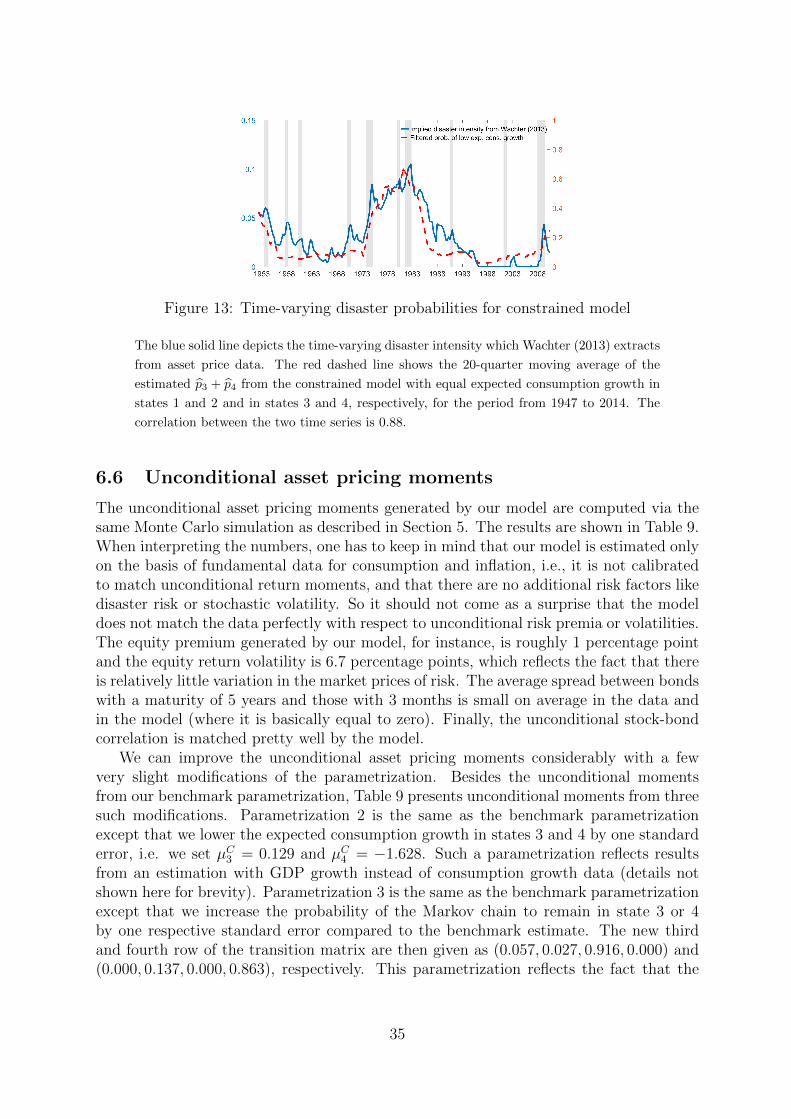
Figure 13: Time-varying disaster probabilities for constrained model

The blue solid line depicts the time-varying disaster intensity which Wachter (2013) extracts

from asset price data. The red dashed line shows the 20-quarter moving average of the

estimated p3 + p4 from the constrained model with equal expected consumption growth in

states 1 and 2 and in states 3 and 4, respectively, for the period from 1947 to 2014. The

correlation between the two time series is 0.88.

6.6 Unconditional asset pricing moments

The unconditional asset pricing moments generated by our model are computed via thesame Monte Carlo simulation as described in Section 5. The results are shown in Table 9.When interpreting the numbers, one has to keep in mind that our model is estimated onlyon the basis of fundamental data for consumption and inflation, i.e., it is not calibratedto match unconditional return moments, and that there are no additional risk factors likedisaster risk or stochastic volatility. So it should not come as a surprise that the modeldoes not match the data perfectly with respect to unconditional risk premia or volatilities.The equity premium generated by our model, for instance, is roughly 1 percentage pointand the equity return volatility is 6.7 percentage points, which reflects the fact that thereis relatively little variation in the market prices of risk. The average spread between bondswith a maturity of 5 years and those with 3 months is small on average in the data andin the model (where it is basically equal to zero). Finally, the unconditional stock-bondcorrelation is matched pretty well by the model.

We can improve the unconditional asset pricing moments considerably with a fewvery slight modifications of the parametrization. Besides the unconditional momentsfrom our benchmark parametrization, Table 9 presents unconditional moments from threesuch modifications. Parametrization 2 is the same as the benchmark parametrizationexcept that we lower the expected consumption growth in states 3 and 4 by one standarderror, i.e. we set µC3 = 0.129 and µC4 = −1.628. Such a parametrization reflects resultsfrom an estimation with GDP growth instead of consumption growth data (details notshown here for brevity). Parametrization 3 is the same as the benchmark parametrizationexcept that we increase the probability of the Markov chain to remain in state 3 or 4by one respective standard error compared to the benchmark estimate. The new thirdand fourth row of the transition matrix are then given as (0.057, 0.027, 0.916, 0.000) and(0.000, 0.137, 0.000, 0.863), respectively. This parametrization reflects the fact that the

35

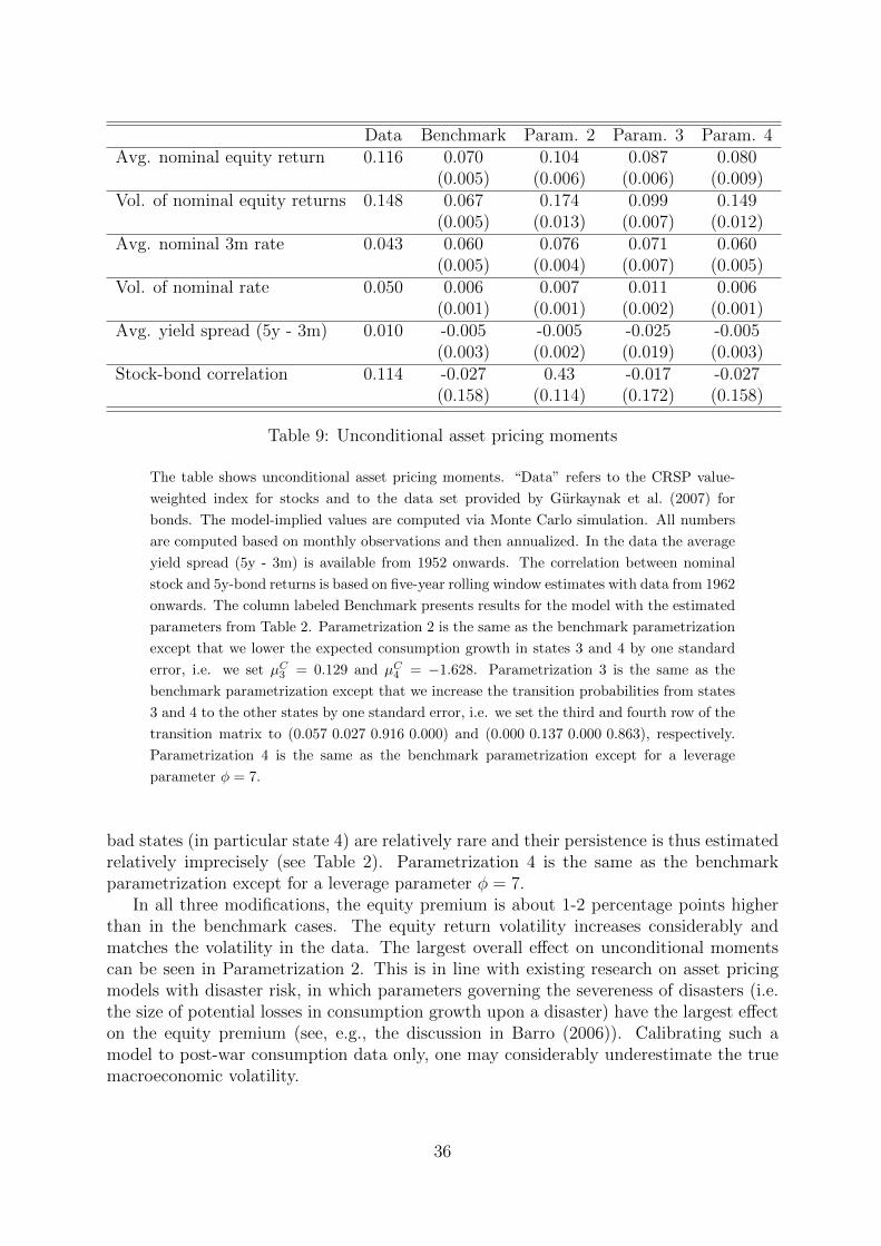
Data Benchmark Param. 2 Param. 3 Param. 4Avg. nominal equity return 0.116 0.070 0.104 0.087 0.080

(0.005) (0.006) (0.006) (0.009)Vol. of nominal equity returns 0.148 0.067 0.174 0.099 0.149

(0.005) (0.013) (0.007) (0.012)Avg. nominal 3m rate 0.043 0.060 0.076 0.071 0.060

(0.005) (0.004) (0.007) (0.005)Vol. of nominal rate 0.050 0.006 0.007 0.011 0.006

(0.001) (0.001) (0.002) (0.001)Avg. yield spread (5y - 3m) 0.010 -0.005 -0.005 -0.025 -0.005

(0.003) (0.002) (0.019) (0.003)Stock-bond correlation 0.114 -0.027 0.43 -0.017 -0.027

(0.158) (0.114) (0.172) (0.158)

Table 9: Unconditional asset pricing moments

The table shows unconditional asset pricing moments. “Data” refers to the CRSP value-

weighted index for stocks and to the data set provided by Gurkaynak et al. (2007) for

bonds. The model-implied values are computed via Monte Carlo simulation. All numbers

are computed based on monthly observations and then annualized. In the data the average

yield spread (5y - 3m) is available from 1952 onwards. The correlation between nominal

stock and 5y-bond returns is based on five-year rolling window estimates with data from 1962

onwards. The column labeled Benchmark presents results for the model with the estimated

parameters from Table 2. Parametrization 2 is the same as the benchmark parametrization

except that we lower the expected consumption growth in states 3 and 4 by one standard

error, i.e. we set µC3 = 0.129 and µC4 = −1.628. Parametrization 3 is the same as the

benchmark parametrization except that we increase the transition probabilities from states

3 and 4 to the other states by one standard error, i.e. we set the third and fourth row of the

transition matrix to (0.057 0.027 0.916 0.000) and (0.000 0.137 0.000 0.863), respectively.

Parametrization 4 is the same as the benchmark parametrization except for a leverage

parameter φ = 7.

bad states (in particular state 4) are relatively rare and their persistence is thus estimatedrelatively imprecisely (see Table 2). Parametrization 4 is the same as the benchmarkparametrization except for a leverage parameter φ = 7.

In all three modifications, the equity premium is about 1-2 percentage points higherthan in the benchmark cases. The equity return volatility increases considerably andmatches the volatility in the data. The largest overall effect on unconditional momentscan be seen in Parametrization 2. This is in line with existing research on asset pricingmodels with disaster risk, in which parameters governing the severeness of disasters (i.e.the size of potential losses in consumption growth upon a disaster) have the largest effecton the equity premium (see, e.g., the discussion in Barro (2006)). Calibrating such amodel to post-war consumption data only, one may considerably underestimate the truemacroeconomic volatility.

36

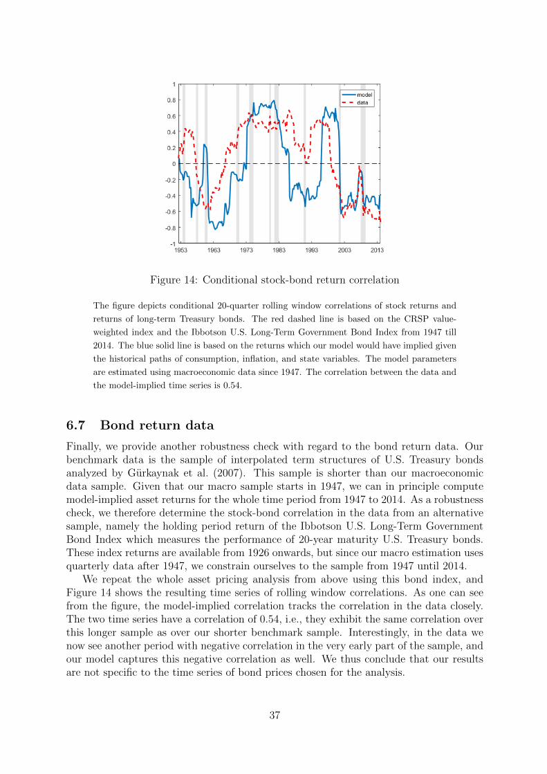
Figure 14: Conditional stock-bond return correlation

The figure depicts conditional 20-quarter rolling window correlations of stock returns and

returns of long-term Treasury bonds. The red dashed line is based on the CRSP value-

weighted index and the Ibbotson U.S. Long-Term Government Bond Index from 1947 till

2014. The blue solid line is based on the returns which our model would have implied given

the historical paths of consumption, inflation, and state variables. The model parameters

are estimated using macroeconomic data since 1947. The correlation between the data and

the model-implied time series is 0.54.

6.7 Bond return data

Finally, we provide another robustness check with regard to the bond return data. Ourbenchmark data is the sample of interpolated term structures of U.S. Treasury bondsanalyzed by Gurkaynak et al. (2007). This sample is shorter than our macroeconomicdata sample. Given that our macro sample starts in 1947, we can in principle computemodel-implied asset returns for the whole time period from 1947 to 2014. As a robustnesscheck, we therefore determine the stock-bond correlation in the data from an alternativesample, namely the holding period return of the Ibbotson U.S. Long-Term GovernmentBond Index which measures the performance of 20-year maturity U.S. Treasury bonds.These index returns are available from 1926 onwards, but since our macro estimation usesquarterly data after 1947, we constrain ourselves to the sample from 1947 until 2014.

We repeat the whole asset pricing analysis from above using this bond index, andFigure 14 shows the resulting time series of rolling window correlations. As one can seefrom the figure, the model-implied correlation tracks the correlation in the data closely.The two time series have a correlation of 0.54, i.e., they exhibit the same correlation overthis longer sample as over our shorter benchmark sample. Interestingly, in the data wenow see another period with negative correlation in the very early part of the sample, andour model captures this negative correlation as well. We thus conclude that our resultsare not specific to the time series of bond prices chosen for the analysis.

37

7 Conclusion

Long-run risk models for asset pricing rest on the key assumption that the conditionaldistribution of consumption growth is time-varying. We provide evidence in favor of thisassumption using a very stylized Markov regime switching model for expected consump-tion growth. While already interesting by itself, this reduced-form approach turns outto be very fruitful when it comes to explaining the joint dynamics of real and nominalasset prices. Augmenting the time series model by inflation as a second macro variablesignificantly alters the estimated regimes. In particular, we find two states in which ex-pected consumption growth is low, one with high expected inflation and one with negativeexpected inflation. Embedding the estimated dynamics in a standard general equilibriumasset pricing model with recursive preferences and learning allows us to match time seriesof aggregate stock return volatility and the stock-bond return correlation.

The basic intuition underlying our results is that low consumption growth tends tooccur together with either very high or very low inflation. In contrast to the volatilityof stock returns, where mainly the overall probability of the two bad states for expectedconsumption growth matters, it is the distinction between the two with respect to expectedinflation which is relevant for the stock-bond return correlation. In the high expectedinflation state, stocks and bonds will both tend to have negative returns, so that theircorrelation will be positive, while in the deflationary state, stocks will still do poorly, butnominal bonds will exhibit positive returns, resulting in a negative correlation betweenthe two types of assets.

Our research design differs substantially from other approaches to calibrate dynamicasset pricing models, where often both asset pricing moments and macroeconomic mo-ments are used to identify the deep parameters of the model. This often leads to aparametrization where macro dynamics are not matched very well. Given the parsi-mony of the research design, in particular the fact that the model is estimated fromtwo macro time series only, we regard our results as evidence that the long-run risk ordisaster risk paradigm in asset pricing can be extended towards an explanation of thetime-varying stock-bond return correlation when the signaling role of inflation is properlyaccounted for. In particular, we also document that our filtered probability of being ina bad consumption growth regime closely tracks the evolution of state variables like the“time-varying disaster risk” which Wachter (2013) obtains through reverse-engineeringfrom asset prices.

In summary, our paper shows that a large part of the variation in asset prices mayactually be attributable to inflation risk, and that the long-run risk model class providesa promising framework to study the link between inflation, consumption growth and bothreal and nominal asset returns.

38

APPENDIX

A. Maximum Likelihood Estimation

The maximum likelihood estimation is based on Hamilton (1994). The parameters of the modeland the transitions probabilities pij are collected in the vector Θ. This vector Θ is estimatedbased on the data YT that is observed until time T . This data forms a T × 2 matrix. LetP (st = j|Θ, Yt) define the probability of state st conditional on all data until t and conditionalon the knowledge of the parameters Θ. The econometrician assigns P (st = j|Θ, Yt) to thepossibility that the observation at time t is generated by state j. These conditional probabilitiesare collected in the n × 1 vector ξt|t, where n denotes the number of states, which is fixedthroughout the entire estimation. We have

ξt|t =ξt|t−1 ηt

1′ · (ξt|t−1 ηt)

ξt+1|t = Q · ξt|t.

Here ηt is the conditional density, whose jth element is

f(yt|st = j; Θ) =1√

2π|Ω|exp

0.5 · (yt − µj)′Ω−1(yt − µj)

,

where yt is an n× 1 vector, µj = (µCj , µπj )′ and Ω = ΣΣ′ where

Σ =

(σC√

1− ρ2 σCρ0 σπ

)Q is the transition probability matrix

Q =

q11 . . . q1n...

. . ....

qn1 . . . qnn

,

denotes element-by-element multiplication, and 1 denotes a vector of ones. The jth elementof the product ξt|t−1 ηt is interpreted as the conditional joint density of yt and st

P (st = j|Θ)× f(yt|st = j; Θ) = p(yt, st = j|Θ).

The density of the observed vector yt is the sum

f(yt|Θ) = 1′ · (ξt|t−1 ηt)

The objective is to find a maximum of the log likelihood function

L(Θ) =

T∑t=1

log f(yt|Θ).

The starting value for the maximization, ξ1|0, is set to 1n · 1.

39

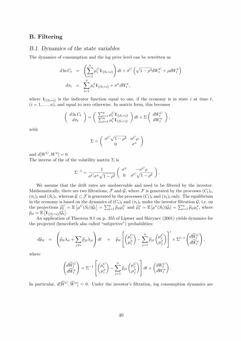
B. Filtering

B.1. Dynamics of the state variables

The dynamics of consumption and the log prive level can be rewritten as

d lnCt =

(n∑i=1

µCi 1St=i

)dt+ σC

(√1− ρ2dWC

t + ρdW πt

)dπt =

n∑i=1

µπi 1St=i + σπdW πt ,

where 1St=i is the indicator function equal to one, if the economy is in state i at time t,(i = 1, . . . , n), and equal to zero otherwise. In matrix form, this becomes(

d lnCtdπt

)=

( ∑ni=1 µ

Ci 1St=i∑n

i=1 µπi 1St=i

)dt+ Σ

(dWC

t

dW πt

),

with

Σ =

(σC√

1− ρ2 σCρ0 σπ

)and d[WC ,W π] = 0.The inverse of the of the volatility matrix Σ is

Σ−1 =1

σCσπ√

1− ρ2

(σπ −σCρ0 σC

√1− ρ2

).

We assume that the drift rates are unobservable and need to be filtered by the investor.Mathematically, there are two filtrations, F and G, where F is generated by the processes (Ct)t,(πt)t and (St)t, whereas G ⊂ F is generated by the processes (Ct)t and (πt)t only. The equilibriumin the economy is based on the dynamics of (Ct)t and (πt)t under the investor filtration G, i.e. onthe projections µCt = E

[µC(St)|Gt

]=∑n

i=1 pitµCi and µπt = E [µπ(St)|Gt] =

∑ni=1 pitµ

πi , where

pit = E[1St=i|Gt

].

An application of Theorem 9.1 on p. 355 of Liptser and Shiryaev (2001) yields dynamics forthe projected (henceforth also called “subjective”) probabilities:

dpit =

pitλii +∑j 6=i

pjtλji

dt + pit

(µCiµπi

)−

n∑j=1

pjt

(µCjµπj

)′ × Σ′−1

(dWC

t

dW πt

),

where (dWC

t

dW πt

)= Σ−1

(µCiµπi

)−

n∑j=1

pjt

(µCjµπj

) dt+

(dWC

t

dW πt

).

In particular, d[WC , W π] = 0. Under the investor’s filtration, log consumption dynamics are

40

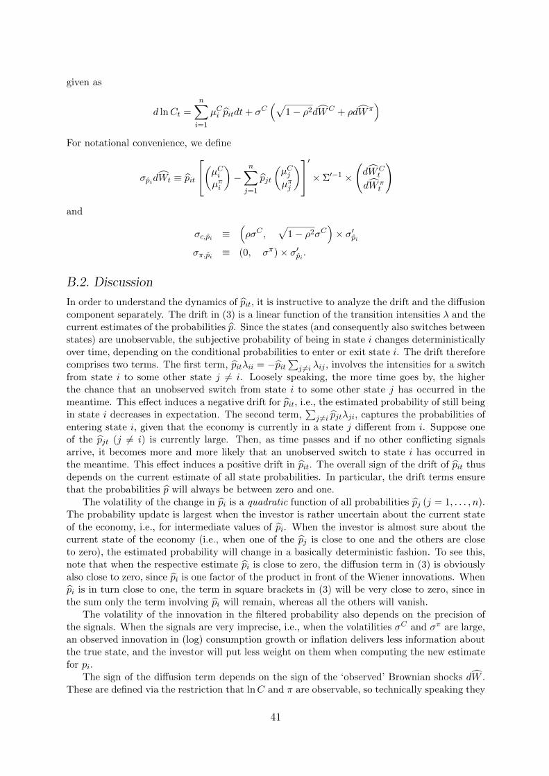
given as

d lnCt =n∑i=1

µCi pitdt+ σC(√

1− ρ2dWC + ρdW π)

For notational convenience, we define

σpidWt ≡ pit

(µCiµπi

)−

n∑j=1

pjt

(µCjµπj

)′ × Σ′−1 ×

(dWC

t

dW πt

)

and

σc,pi ≡(ρσC ,

√1− ρ2σC

)× σ′pi

σπ,pi ≡ (0, σπ)× σ′pi .

B.2. Discussion

In order to understand the dynamics of pit, it is instructive to analyze the drift and the diffusioncomponent separately. The drift in (3) is a linear function of the transition intensities λ and thecurrent estimates of the probabilities p. Since the states (and consequently also switches betweenstates) are unobservable, the subjective probability of being in state i changes deterministicallyover time, depending on the conditional probabilities to enter or exit state i. The drift thereforecomprises two terms. The first term, pitλii = −pit

∑j 6=i λij , involves the intensities for a switch

from state i to some other state j 6= i. Loosely speaking, the more time goes by, the higherthe chance that an unobserved switch from state i to some other state j has occurred in themeantime. This effect induces a negative drift for pit, i.e., the estimated probability of still beingin state i decreases in expectation. The second term,

∑j 6=i pjtλji, captures the probabilities of

entering state i, given that the economy is currently in a state j different from i. Suppose oneof the pjt (j 6= i) is currently large. Then, as time passes and if no other conflicting signalsarrive, it becomes more and more likely that an unobserved switch to state i has occurred inthe meantime. This effect induces a positive drift in pit. The overall sign of the drift of pit thusdepends on the current estimate of all state probabilities. In particular, the drift terms ensurethat the probabilities p will always be between zero and one.

The volatility of the change in pi is a quadratic function of all probabilities pj (j = 1, . . . , n).The probability update is largest when the investor is rather uncertain about the current stateof the economy, i.e., for intermediate values of pi. When the investor is almost sure about thecurrent state of the economy (i.e., when one of the pj is close to one and the others are closeto zero), the estimated probability will change in a basically deterministic fashion. To see this,note that when the respective estimate pi is close to zero, the diffusion term in (3) is obviouslyalso close to zero, since pi is one factor of the product in front of the Wiener innovations. Whenpi is in turn close to one, the term in square brackets in (3) will be very close to zero, since inthe sum only the term involving pi will remain, whereas all the others will vanish.

The volatility of the innovation in the filtered probability also depends on the precision ofthe signals. When the signals are very imprecise, i.e., when the volatilities σC and σπ are large,an observed innovation in (log) consumption growth or inflation delivers less information aboutthe true state, and the investor will put less weight on them when computing the new estimatefor pi.

The sign of the diffusion term depends on the sign of the ‘observed’ Brownian shocks dW .These are defined via the restriction that lnC and π are observable, so technically speaking they

41

have to be adapted to both F and G, which implies µ(St)dt+ ΣdWt = µtdt+ ΣdWt.

C. Solution of the Model with Partial Information

C.1. Wealth-consumption ratio

The indirect utility function of the investor is given by

J(Ct, p1t, . . . , pnt) = Et

[∫ ∞t

f(Cs, J(Cs, p1s, . . . , pns)) ds

].

J (Ct, p1t, . . . , pnt) +∫ t0 f (Cs, J(Cs, p1s, . . . , pns)) ds is a martingale, therefore we have the Bell-

man equation

E[dJ(Ct, p1t, . . . , pnt) + f(Ct, J(Ct, p1t, . . . , pnt)) dt] = 0,

or, equivalently,

AJ(Ct, p1t, . . . , pnt)

J(Ct, p1t, . . . , pnt)+f(Ct, J(Ct, p1t, . . . , pnt))

J(Ct, p1t, . . . , pnt)= 0, (C.1)

where A is the infinitesimal generator. The aggregator function is given by

f(C, J) =βC

1− 1ψ(

1− 1ψ

) [(1− γ)J

] 1θ−1− βθJ.

We conjecture a functional form for J :

J(Ct, p1t, . . . , pnt) =C1−γt

1− γ

(βev(p1t,...,pnt)

)θwhere in the end v will turn out to be the log wealth-consumption ratio. This functional formtogether with the definition of f(C, J) implies

f(C, J)

J= θe−v − θβ.

With I ≡ ev the partial derivatives of J (denoted by subscripts) are

Jc = C−γ (βev)θ

Jcc = −γC−γ−1 (βev)θ

Jpi =C1−γ

1− γβθθIθ−1Ipi

Jpipj =C1−γ

1− γβθθ

[(θ − 1)Iθ−2I2pi + IpipjI

θ−1]

Jcpi = C−γβθθIθ−1Ipi ,

42

resulting in

JcJdCt = (1− γ)

n∑i=1

µCi pitdt+1

2(σC)2(1− γ)dt+ (1− γ)σC

(√1− ρ2dWC

t + ρdW πt

)Jccd[C,C]t

J= (σC)2(−γ)(1− γ)dt

Jcpid[C, pi]t

J= θ(1− γ)

IpiIσc,pidt

Jpidpit

J= θ

IpiIdpit

Jpipjd[pi, pj ]t

J=

1

2θd[pi, pj ]t

[(θ − 1)

(IpiI

)2

+IpipjI

].

Plugging everything into (C.1) results in the following partial differential equation for I:

0 =

[(1− γ)

n∑i=1

µCi pit +1

2(1− γ)2(σC)2 − βθ

]+ θI−1 (C.2)

+

n−1∑i=1

θIpitI

piλii +

n∑j=1j 6=i

pjtλji

+

n−1∑i=1

θ(1− γ)IpiIσc,pi

+1

2

n−1∑i=1

n−1∑j=1

θ

[(θ − 1)

(IpiIpjI

)+IpipjI

]σpiσ

′pj,

There are n − 1 state variables due to the restriction∑n

i=1 pit = 1. We solve the PDE with aChebyshev approximation similar to Benzoni et al. (2011). We guess the following functionalform for I as a function of the vector p = (p1, p2, ..., pn−1) with:

I(p) = exp(B(p)) (C.3)

B(p) =

d∑j=0

αjTj(p),

where the Tj(p) are multivariate Chebyshev polynomials. For the interval [−1, 1], the univariateChebyshev polynomials are defined recursively via

T0(x) = 1

T1(x) = x

Td+1(x) = 2xTd(x)− Td−1(x).

Univariate Chebyshev polynomials for the general interval [a, b] are given by transformations

Td

(2x− b− ab− a

).

Multivariate versions of the Chebyshev polynomials are defined as sums of products of the

43

univariate ones. The derivatives of the guess in (C.3) are

Ipi = eB(p)Bpi = eB(p)d∑j=1

αj∂Tj∂pi

(p)

Ipipj = eB(p)[(Bpi)

2 +Bpipj]

= eB(p)

d∑j=1

αj∂Tj∂pi

(p)

2

+

d∑j=2

αj∂2Tj∂pi∂pj

(p)

.Plugging the partial derivatives into (C.2) gives

0 =

[(1− γ)

n∑i=1

µCi pi +1

2(1− γ)2(σC)2 − βθ

]+ e−

∑dj=0 αjTj(p)θ

+n−1∑i=1

θ

d∑j=1

αj∂Tj∂pi

(p)

pitλii +

n∑j=1j 6=i

pjtλji

+n−1∑i=1

θ(1− γ)

d∑j=1

αj∂Tj∂pi

(p)

σc,pi

+1

2

n−1∑i=1

n−1∑k=1

θ

(θ − 1)

d∑j=1

αj∂Tj∂pi

(p)

d∑j=1

αj∂Tj∂pk

(p) +d∑j=2

αj∂2Tj∂pi∂pk

(p)

σpiσ′pk .This equation is defined on the simplex ∆n−1. We partition this simplex by choosing grid pointsaccording to the Chebyshev methodology. Evaluating the equation on every grid point leavesus with a number of algebraic equations, whose solution gives the Chebyshev coefficients αj .For the multivariate Chebyshev polynomials we choose the order of d = 4. We have also triedhigher values for d but the solution remained unchanged.

C.2. Pricing kernel

The pricing kernel is given by

ξt = exp

(∫ t

0−βθ − (1− θ)I−1(ps)ds

)C−γt (I(pt))

θ−1

with dynamics

dξtξt

= −βθdt− (1− θ)I−1 dt− γ dCtCt

+1

2γ2(σC)2dt

− (1− θ)n−1∑i=1

IpiIdpit +

1

2

n−1∑i=1

n−1∑j=1

(θ − 1)

[IpipjI

+ (θ − 2)

(IpiIpjI2

)]σpiσ

′pjdt

− γ(θ − 1)

n−1∑i=1

IpiIσc,pidt,

44

where p = (p1, p2, ..., pn). For later use, we abbreviate the drift term as

µξ,t ≡ −βθ − (1− θ)I−1(pt) − γn∑i=1

µCi pit +1

2γ2(σC)2 −

n−1∑i=1

(1− θ)IpiI

pitλii +

n∑j=1j 6=i

pjtλji

+

1

2

n−1∑i=1

n−1∑j=1

(θ − 1)[IpipjI

+ (θ − 2)

(IpiIpjI2

)]σpiσ

′pj

− γ(θ − 1)

n−1∑i=1

IpiIσc,pi .

C.3. Price-dividend ratio

We want to price a claim on levered consumption. Under the investor’s filtration, dividendsfollow the process

d lnDt = µdt+ φ

(n∑i=1

(µCi − µ)pit

)dt+ φσC

(√1− ρ2dWC

t + ρdW πt

).

Let ω denote the log price-dividend ratio. For g(ξ,D, ω) ≡ ξDeω, the Feynman-Kac formulayields

Ag(ξ,D, ω)

g(ξ,D, ω)+ e−ω = 0. (C.4)

Ito’s Lemma gives

Agtgt

= µξ,t + µD,t + µω,t +1

2

d[ω]tdt

+d [ξ,D]tξDdt

+d [ω,D]tDdt

+d [ω, ξ]tξdt

.

Another application of Ito’s Lemma leads to

dωt =n−1∑i=1

ωpidpit +1

2

n−1∑i=1

n−1∑j=1

ωpipjσpiσ′pjdt

where the subscripts denote partial derivatives with respect to the state variables pi. We canrewrite the drift of ω as a function of the derivatives ωpi and ωpi,pj and the state variables pi:

µω,t =

n−1∑i=1

ωpi

pitλii +

n∑j=1j 6=i

pjtλji

+1

2

n−1∑i=1

n−1∑j=1

ωpipjσpiσ′pj.

45

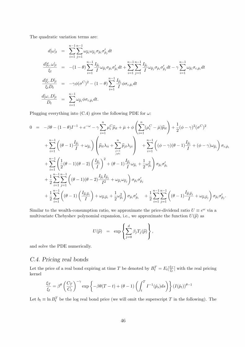
The quadratic variation terms are:

d[ω]t =

n−1∑i=1

n−1∑j=1

ωpiωpjσpiσ′pjdt

d[ξ, ω]tξt

= −(1− θ)n−1∑i=1

IpiIωpiσpiσ

′pidt+

n−1∑i=1

n−1∑j=1

IpiIωpjσpiσ

′pjdt− γ

n−1∑i=1

ωpiσc,pidt

d[ξ,D]tξtDt

= −γφ(σC)2 − (1− θ)n−1∑i=1

IpiIφσc,pidt

d[ω,D]tDt

=

n−1∑i=1

ωpiφσc,pidt.

Plugging everything into (C.4) gives the following PDE for ω:

0 = −βθ − (1− θ)I−1 + e−ω − γn∑i=1

µCi pit + µ+ φ

(n∑i=1

(µCi − µ)pit

)+

1

2(φ− γ)2(σC)2

+

n−1∑i=1

((θ − 1)

IpiI

+ ωpi

)pitλii +n∑j=1j 6=i

pjtλji

+n−1∑i=1

((φ− γ)(θ − 1)

IpiI

+ (φ− γ)ωpi

)σc,pi

+

n−1∑i=1

(1

2(θ − 1)(θ − 2)

(IpiI

)2

+ (θ − 1)IpiIωpi +

1

2ω2pi

)σpiσ

′pi

+1

2

n−1∑i=1

n−1∑j=1

((θ − 1)(θ − 2)

IpiIpjI2

+ ωpiωpj

)σpiσ

′pj

+1

2

n−1∑i=1

((θ − 1)

(IpipiI

)+ ωpipi +

1

2ω2pi

)σpiσ

′pi

+1

2

n−1∑i=1

n−1∑j=1

((θ − 1)

IpipjI

+ ωpipj

)σpiσ

′pj.

Similar to the wealth-consumption ratio, we approximate the price-dividend ratio U ≡ eω via amultivariate Chebyshev polynomial expansion, i.e., we approximate the function U(p) as

U(p) = exp

d∑j=0

βjTj(p)

,

and solve the PDE numerically.

C.4. Pricing real bonds

Let the price of a real bond expiring at time T be denoted by BTt = Et[

ξTξt

] with the real pricingkernel

ξTξt

= βθ(CTCt

)−γexp

−βθ(T − t) + (θ − 1)

(∫ T

tI−1(ps)ds

)(I(pt))

θ−1

Let bt ≡ lnBTt be the log real bond price (we will omit the superscript T in the following). The

46

Feynman-Kac formula applied to H(ξt, bt) = ξtebt yields the partial differential equation:

0 = AH = µξ,t + µb,t +1

2

d[b]tdt

+d[ξ, b]tξtdt

, (C.5)

where µξ and µb are the drifts of the processes ξt and bt respectively. The dynamics of bt are

dbt =∂bt∂tdt+

n−1∑i=1

bpidpit +1

2

n−1∑i=1

n−1∑j=1

bpipjσpiσ′pjdt.

Plugging everything into (C.5) gives the following PDE for bt:

0 = −βθ − (1− θ)I−1 − γn∑i=1

µCi pit +1

2γ2(σC)2 +

∂bt∂t

+

n−1∑i=1

((θ − 1)

IpiI

+ bpi

)pitλii +

n∑j=1j 6=i

pjtλji

− γ(θ − 1)

n−1∑i=1

IpiIσc,pi − γ

n−1∑i=1

ωpiσc,pi

+

n−1∑i=1

(1

2(θ − 1)(θ − 2)

(IpiI

)2

+ (θ − 1)IpiIbpi +

1

2b2pi

)σpiσ

′pi

+1

2

n−1∑i=1

n−1∑j=1

((θ − 1)(θ − 2)

IpiIpjI

+ bpibpj

)σpiσ

′pj

+n−1∑i=1

1

2

((θ − 1)

(IpipiI

)+ bpipi +

1

2b2pi

)σpiσ

′pi

+1

2

n−1∑i=1

n−1∑j=1

((θ − 1)

IpipjI

+ bpipj

)σpiσ

′pj.

We approximate the bond price ebt at each time point t by a multivariate Chebyshev polynomial,i.e.,

bt =n∑j=0

α(T )j,t Tj(p).

Note that the PDE for the bond price involves a time derivative. We use an explicit Eulerdiscretization for this time derivative and solve the PDE recursively backwards in time, starting

from the boundary condition bT = 0, i.e. α(T )j,T = 0 for j = 0, . . . , n.

C.5. Pricing nominal bonds

Let the price of the nominal bond maturing at time T be denoted by BT,$t with

BT,$t = Et

[ξ$Tξ$t

]

= Et

[ξTξt

eπt

eπT

],

where ξ$t ≡ ξte−πt is the nominal pricing kernel. Define b$t ≡ lnBT,$

t (we again omit the

superscript T in the following). Then the Feynman-Kac formula applied to H(ξ$t , b$t ) = ξ$t e

b$t

47

yields the partial differential equation

0 = AH = µξ$,t + µb$,t +1

2

d[b$t ]

dt+d[ξ$, b$]t

ξ$t dt, (C.6)

where µξ$ and µb$ are drifts of the processes ξ$t and b$t respectively. Notice that

dξ$tξ$t

=dξtξt− dπt +

1

2d[π]t −

d[ξ, π]tξt

.

The dynamics of b$t are

db$t =∂b$t∂t

dt+n−1∑i=1

b$pidpit +1

2

n−1∑i=1

n−1∑j=1

b$pipjσpiσ′pjdt.

Plugging everything into (C.6) yields the following PDE for b$t :

0 = −βθ − (1− θ)I−1 − γn∑i=1

µCi pit +1

2γ2(σC)2 +

∂b$t∂t−

n∑i=1

µπi pit +1

2(σπ)2 + γρσCσπ

+

n−1∑i=1

((θ − 1)

IpiI

+ bp$i

)pitλii +n∑j=1j 6=i

pjtλji

− γ(θ − 1)

n−1∑i=1

IpiIσc,pi − γ

n−1∑i=1

b$piσc,pi − (θ − 1)

n−1∑i=1

IpiIσπ,pi −

n−1∑i=1

b$piσπ,pi

+

n−1∑i=1

(1

2(θ − 1)(θ − 2)

(IpiI

)2

+ (θ − 1)IpiIb$pi +

1

2(b$pi)

2

)σpiσ

′pi

+1

2

n−1∑i=1

n−1∑j=1

((θ − 1)(θ − 2)

IpiIpjI

+ b$pib$pj

)σpiσ

′pj

+1

2

n−1∑i=1

((θ − 1)

(IpipiI

)+ b$pipi +

1

2(b$pi)

2

)σpiσ

′pi

+1

2

n−1∑i=1

n−1∑j=1

((θ − 1)

IpipjI

+ b$pipj

)σpiσ

′pj.

Again, this PDE involves a time derivative. As for the prices of real bonds, we approximate

eb$t at each time point t by multivariate Chebyshev polynomials, use an explicit Euler discretiza-

tion for this time derivative and solve the PDE recursively backwards in time, starting from theboundary condition b$T = 0.

48

D. Solution of the Model with Full Information

The dynamics of consumption and the log prive level are

d lnCt =

(n∑i=1

µCi 1St=i

)dt+ σC

(√1− ρ2dWC

t + ρdW πt

)dπt =

n∑i=1

µπi 1St=i + σπdW πt ,

For ease of notation, we relabel the indicator variable as pi,t = 1St=i. These are the statevariables in a model in which the representative agent perfectly knows the state of the economyat every point in time. The dynamics of these state variables are

dpi,t = −pi,tdNi,i + (1− pi,t)∑j 6=i

dNj,i

where the counting process Nj,i counts transitions from state j to state i and has the intensityλj,i. The counting process Ni,i counts the transitions from state i to any other state j 6= i andhas the intensity

∑j 6=i λi,j . These dynamics imply that the state variables almost surely only

take the values 0 and 1.The indirect utility function of the investor is given by

J(Ct, p1t, . . . , pnt) = Et

[∫ ∞t

f(Cs, J(Cs, p1s, . . . , pns)) ds

].

With the same reasoning as in the incomplete information economy (i.e. defining the indirectutility function, setting up the Bellman equation, conjecturing the same functional form forthe indirect utility function) and after some simplifications, we arrive at the following algebraicequations (one equation for each state i) for the four unknowns vi (the log wealth-consumptionratios in each state i):

0 =

[(1− γ)µCi +

1

2(1− γ)2(σC)2 − βθ

]+ θe−vi +

∑j 6=i

λij ·(eθ(vj−vi) − 1

).

The proof is only a very slight modification of the proof in Appendix A of Branger et al. (2016).Similarly, for the log price-dividend ratio ωi of the equity claim, we get the equations (one foreach state i):

0 = −βθ − (1− θ)e−vi + e−ωi − γµCi + µ+ φ(µCi − µ

)+

1

2(φ− γ)2(σC)2

+∑j 6=i

λij ·(e(θ−1)(vj−vi) · eωj−ωi − 1

).

For the prices of nominal bonds b$i we get the four ordinary differential equations

0 = −βθ − (1− θ)e−vi − γµCi +1

2γ2(σC)2 +

∂b$i∂t− µπi +

1

2(σπ)2 + γρσCσπ

+∑j 6=i

λij ·(e(θ−1)(vj−vi) · eb

$j−b

$i − 1

).

49

REFERENCES

Ang, A. and M. Ulrich (2012). Nominal bonds, real bonds and equity. Working Paper .

Backus, D., M. Chernov, and I. Martin (2011). Disasters implied by equity index options.Journal of Finance 66 (6), 1969–2012.

Baele, L., G. Bekaert, and K. Inghelbrecht (2010). The determinants of stock and bondreturn comovements. Review of Financial Studies 23 (6), 2374–2428.

Balduzzi, P. and C. Lan (2016). Survey forecasts and the time-varying second momentsof stock and bond returns. Working Paper .

Bansal, R., D. Kiku, and A. Yaron (2012). An empirical evaluation of the long-run risksmodel for asset prices. Critical Finance Review 1 (1), 183–221.

Bansal, R., D. Kiku, and A. Yaron (2016). Risks for the Long Run: Estimation withTime Aggregation. Journal of Monetary Economics 82 (1), 52–69.

Bansal, R. and I. Shaliastovich (2013). A long-run risks explanation of predictabilitypuzzles in bond and currency markets. Review of Financial Studies 26 (1), 1–33.

Bansal, R. and A. Yaron (2004, August). Risks for the long run: A potential resolutionof asset pricing puzzles. Journal of Finance 59 (4), 1481–1509.

Barro, R. (2006). Rare disasters and asset markets in the twentieth century. QuarterlyJournal of Economics 121 (3), 823–866.

Barro, R. (2009). Rare disasters, asset prices, and welfare costs. American EconomicReview 99 (1), 243–64.

Basak, S. and H. Yan (2010). Equilibrium asset prices and investor behavior in thepresence of money illusion. Review of Economic Studies 77 (3), 914–936.

Beeler, J. and J. Campbell (2012). The long-run risks model and aggregate asset prices:An empirical assessment. Critical Finance Review 1 (1), 142–182.

Benzoni, L., P. Collin-Dufresne, and R. S. Goldstein (2011). Explaining asset pricingpuzzles associated with the 1987 market crash. Journal of Financial Economics 101 (3),552–573.

Boons, M., F. de Roon, F. Duarte, and M. Szymanowska (2017). Time-varying inflationrisk and the cross-section of stock returns. Working Paper .

Branger, N., H. Kraft, and C. Meinerding (2016). The dynamics of crises and the equitypremium. Review of Financial Studies 29 (1), 232–270.

Burkhardt, D. and H. Hasseltoft (2012). Understanding asset correlations. WorkingPaper .

Campbell, J., C. Pflueger, and L. Viceira (2018). Monetary policy drivers of bond andequity risks. Working Paper .

50

Campbell, J., A. Sunderam, and L. Viceira (2017). Inflation bets or deflation hedges? thechanging risks of nominal bonds. Critical Finance Review 6 (2), 263–301.

Chen, H., W. Dou, and L. Kogan (2017). Measuring the “dark matter” in asset pricingmodels. Working Paper .

Chen, H., S. Joslin, and N.-K. Tran (2012). Rare disasters and risk sharing. Review ofFinancial Studies 25, 2189–224.

Constantinides, G. (2008). Comment on “macroeconomic crises since 1870” by barro andursua. Brookings Papers on Economic Activity , 341–50.

Constantinides, G. and A. Ghosh (2011). Asset pricing tests with long-run risk in con-sumption growth. Review of Asset Pricing Studies 1 (1), 96–136.

Constantinides, G. and A. Ghosh (2017). What information drives asset prices? WorkingPaper .

Croce, M., M. Lettau, and S. Ludvigson (2012). Investor information, long-run risk andthe term structure of equity. Review of Financial Studies 28 (3), 706–742.

David, A. and P. Veronesi (2013). What ties return volatilities to price valuations andfundamentals. Journal of Political Economy 121 (4), 682–746.

Detemple, J. B. (1986). Asset pricing in a production economy with incomplete informa-tion. Journal of Finance 41, 383–391.

Drechsler, I. (2013). Uncertainty, time-varying fear and asset prices. Journal of Fi-nance 68 (5), 1843–1889.

Duffie, D. and L. G. Epstein (1992a). Asset pricing with stochastic differential utility.Review of Financial Studies 5 (3), 411–436.

Duffie, D. and L. G. Epstein (1992b, March). Stochastic differential utility. Economet-rica 60 (2), 353–394.

Ehling, P., M. Gallmeyer, C. Heyerdahl-Larsen, and P. Illeditsch (2018). Disagreementabout inflation and the yield curve. Journal of Financial Economics 127 (3), 459–484.

Eraker, B. (2008). Affine general equilibrium models. Management Science 54 (12), 2068–2080.

Eraker, B., I. Shaliastovich, and W. Wang (2016). Durable goods, inflation risk andequilibrium asset prices. Review of Financial Studies 29 (1), 193–231.

Ermolov, A. (2018). Time-varying risks of nominal bonds: How important are macroeco-nomic shocks. Working Paper .

Fleckenstein, M., F. Longstaff, and H. Lustig (2016). Deflation risk. forthcoming: Reviewof Financial Studies .

51

Gabaix, X. (2012). Variable rare disasters: An exactly solved framework for ten puzzlesin macro-finance. Quarterly Journal of Economics 127 (2), 645–700.

Gurkaynak, R. S., B. Sack, and J. H. Wright (2007, November). The u.s. treasury yieldcurve: 1961 to the present. Journal of Monetary Economics 54, 2291–2304.

Hamilton, J. D. (1994). Time series analysis. Princeton University Press.

Hasseltoft, H. (2012). Stocks, bonds, and long-run consumption risks. Journal of Financialand Quantitative Analysis 47 (2), 309–332.

Julliard, C. and A. Ghosh (2012). Can rare events explain the equity premium puzzle?Review of Financial Studies 25, 3037–3076.

Liptser, R. and A. Shiryaev (2001). Statistics of Random Processes I: General Theory.Springer-Verlag, Berlin.

Marfe, R. (2015). Labor rigidity, inflation risk and bond returns. Working Paper .

Newey, W. K. and K. D. West (1987). A simple, positive semi-definite, heteroskedasticityand autocorrelation consistent covariance matrix. Econometrica 55 (3), 703–708.

Ortu, F., A. Tamoni, and C. Tebaldi (2013). Long-run risk and the persistence of con-sumption shocks. Review of Financial Studies 26 (11), 2876–2915.

Piazzesi, M. and M. Schneider (2006). Equilibrium yield curves. NBER MacroeconomicsAnnual , 389–442.

Rietz, T. (1988). The equity premium: A solution. Journal of Monetary Economics 22 (1),117–31.

Schmeling, M. and A. Schrimpf (2011). Expected inflation, expected stock returns, andmoney illusion: What can we learn from survey expectations? European EconomicReview 55 (5), 702–719.

Schorfheide, F., D. Song, and A. Yaron (2018). Identifying long-run risks: A bayesianmixed-frequency approach. Econometrica 86 (2), 617–654.

Song, D. (2017). Bond market exposures to macroeconomic and monetary policy risks.Review of Financial Studies 30 (8), 2761–2817.

Tsai, J. and J. Wachter (2015). Disaster risk and its implications for asset pricing. AnnualReview of Financial Economics 7, 219–252.

Wachter, J. (2006). A consumption-based model of the term structure of interest rates.Journal of Financial Economics 79 (2), 365–399.

Wachter, J. (2013). Can time-varying risk of rare disasters explain aggregate stock marketvolatility? Journal of Finance 68 (3), 987–1035.

52