56TH INTERNATIONAL SCIENTIFIC COLLOQUIUM Ilmenau University of Technology, 12 – 16 September 2011

URN: urn:nbn:gbv:ilm1-2011iwk:5

©2011 – TU Ilmenau

Extreme Bending of Spring Steel Wire - Theory and Experiment

M. Weiß / J. Steigenberger / V. Geinitz / P. Beyer

Ilmenau University of Technology

ABSTRACT In this paper we report on experimental investigations of spring-steel wire. Spring steel-wire is a high quality product of the wire industry with outstanding mechanical properties which should ensure that components such as compression springs with smallest mass produce high spring forces. The experimental set-up is a three-point bending test rig. Aim of the experiments was (1) to find the limit of extreme elastic bending of wires - the spring bending limit, and (2) to determine the elasticity modulus of spring-steel via bending, thereby using also test objects having a pre-curvature. A mathematical framework necessary for quantitative interpretation of the experiments is presented, and numerical results are given in a universally utilizable form. What is new is the full numerical solution of the exact differential equation of the elastic line by a Maple program. Index Terms – spring-steel wire, extreme bending of elastic rods, nonlinear bending theory, MAPLE-application, three-point bending test rig, modulus of elasticity, wire with pre-curvature

0. INTRODUCTION For more than four decades research has been carried at the Ilmenau University of Technology on springs and spring materials. One current topic regards “function- and production-relevant parameters for spring steel wire and steel strips” [1]. Initial results are presented on this topic below. In this paper we report on experimental investigations of spring-steel wire. Spring steel-wire is a high quality product of the wire industry with outstanding mechanical properties which should ensure that components such as compression springs with smallest mass guarantee high spring forces. The experimental set-up is a three-point bending test rig. Aim of the experiments was (1) to find the limit of extreme elastic bending of wires - the spring bending limit, and (2) to determine the elasticity module of spring-steel via bending, thereby using also test objects having a pre-curvature. A mathematical framework necessary for quantitative interpretation of the experiments is presented, and numerical results are given in a universally utilizable form. What is new is the full numerical solution of the exact differential equation of the elastic line by a Maple program. For the experiments we used the following three materials: Oil-tempered spring-steel wire: VDSiCr - Oteva 70 SC RD40 S: diameters: 3 mm and 6 mm; Patented drawn spring-steel wire: SH, diameter: 3 mm; Stainless spring-steel wire: 1.4310, diameter: 6 mm.

URN (Paper): urn:nbn:de:gbv:ilm1-2011iwk-020:5

2

In order to calculate the expected bending deformations, it is first necessary to determine the elasticity modulus of the three materials. The test principle is always the same: a three-point bending test rig is used to measure force-displacement curves for small elastic deformations. The slope of these curves is proportional to the elasticity modulus. Since bending springs are exposed to large deformations in practice, it is necessary to be able to calculate the expected large elastic deformations for a specific load. This requires the integration of the exact differential equation for bending. In order to remain within the load carrying limits, the allowable maximum outer fiber stress must both be known as well as able to be checked. The experiments to determine the spring bending limit provide the necessary material parameters and the theoretical results allow the exact outer fiber stresses to be calculated. Therefore the following tasks needed to be completed:

1. Development of a theory to determine the elasticity modulus, the gradient of the bending line, the curve of the bending stress and the spring bending limit based on experimental data

2. Construction of a three-point bending test rig and carrying out of corresponding measurements

3. Evaluation of measurement results using the theory.

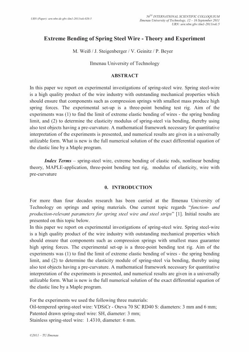
0.1 Experimental Set-up To determine the mechanical properties in bending, a three-point bending test rig is required [5]. Fig. 1 shows the newly developed experimental set-up. The sample under test is a stainless spring-steel wire with a wire diameter of about 6 mm. Fig. 1: Three-point bending test rig Details of the force measuring system: KAP-E-D, measuring system 200 N, class 0.1, manufacturer: AST Details of the positioning system: Mechanical basement: manufacturer: ZWICK, type 1446, 10 kN

force measuring system

positioning system

3

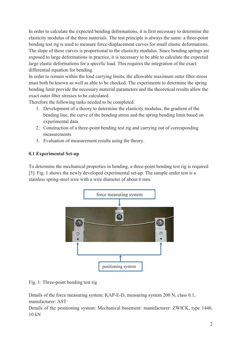
Control system: Manufacturer: DOLI, type ETC 100 The physical model for the three-point bending test shows Fig. 2.

x

y

A BL

F=-Fey

|F|=F

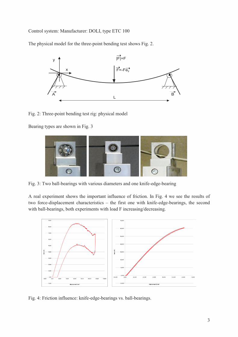
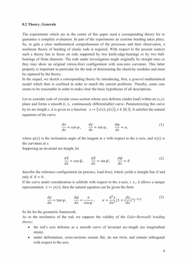
Fig. 2: Three-point bending test rig: physical model Bearing types are shown in Fig. 3 Fig. 3: Two ball-bearings with various diameters and one knife-edge-bearing A real experiment shows the important influence of friction. In Fig. 4 we see the results of two force-displacement characteristics – the first one with knife-edge-bearings, the second with ball-bearings, both experiments with load F increasing/decreasing. Fig. 4: Friction influence: knife-edge-bearings vs. ball-bearings.

4

0.2 Theory, Generals The experiments which are in the center of this paper need a corresponding theory for to guarantee a complete evaluation. In part of the experiments an extreme bending takes place. So, to gain a clear mathematical comprehension of the processes and their observation, a nonlinear theory of bending of elastic rods is required. With respect to the present context such a theory has to focus on rods supported by two knife-edge-bearings or by two ball-bearings of finite diameter. The rods under investigation might originally be straight ones or they may show an original (stress-free) configuration with non-zero curvature. This latter property is important in particular for the task of determining the elasticity modulus and must be captured by the theory. In the sequel, we sketch a corresponding theory by introducing, first, a general mathematical model which then is confined in order to match the current problems. Thereby, some care seems to be reasonable in order to make clear the basic hypotheses of all descriptions. Let us consider rods of circular cross-section whose axis deforms (under load) within an (x,y)-plane and forms a smooth (i. e., continuously differentiable) curve. Parameterizing this curve by its arc-length s, it is given as a function . It satisfies the natural equations of the curve

(1)

where is the inclination angle of the tangent at with respect to the -axis, and is the curvature at . Supposing an invariant arc-length, let

(2)

describe the reference configuration (in practice, load-free), which yields a straight line if and only if . If the curve under consideration is schlicht with respect to the -axis, i. e., it allows a unique representation , then the natural equation can be given the form

(3)

So far for the geometric framework. As to the mechanics of the rod, we suppose the validity of the Euler-Bernoulli bending theory:

� the rod’s axis deforms as a smooth curve of invariant arc-length (no longitudinal strain)

� under deformation, cross-sections remain flat, do not twist, and remain orthogonal with respect to the axis,

5

� the local strain (due to the mutual slope of neighbored cross-sections) implies stress following Hooke’s law ( : physical linearity).

The outcome of these hypotheses is a linear distribution of the stress over the cross-sections with zero resultant force and a resultant moment governed by the well known material law (rheological equation)

(4)

denotes the elasticity modulus of the material, denotes the equatorial moment of inertia of the cross-section, is the bending stiffness (assumed constant). Now the procedure to solve equilibrium problems is mainly based on (1) and (4), and therefore essentially always the same. Assume bending stiffness, external load, kind of support, and the load-free configuration to be given. In a general configuration, determine through appropriate dissection of the rod from local equilibrium equations. Thereby appears as a function of and certain statical parameters (given loads: known, reactions to supports: in general unknown). Then, (4) yields as an analogous function, and (1) represents a system of ordinary differential equations which, together with well-defined boundary conditions (supports!), determine the functions and (configuration under load) and the unknown parameters as well. It is this procedure, that is worked through in slight specifications for the problems concerning the experiments. The physical model of a three-point bending test rig is shown in Fig. 2. We shall give mathematical descriptions for such tests using different designs of the supports. Of course, any model should not only be valid just for one particular implementation with concrete data of the investigation object and the experimental set-up. To this end we use an appropriate standardization, that means, for every relevant geometrical and physical quantity we introduce units of measurement which fit the current problem data. This is done as follows. Denote the geometric / physical quantities by upper-case letters, the corresponding (dimensionless) variables by the respective lower-case letters. System data used for composing the units are .

6

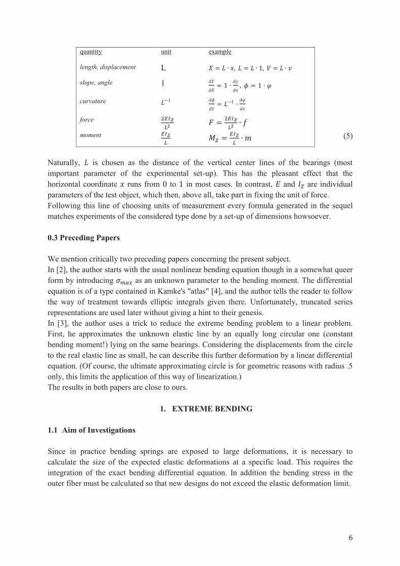
quantity unit example

length, displacement L

slope, angle 1

curvature

force

moment (5)

Naturally, is chosen as the distance of the vertical center lines of the bearings (most important parameter of the experimental set-up). This has the pleasant effect that the horizontal coordinate runs from to in most cases. In contrast, and are individual parameters of the test object, which then, above all, take part in fixing the unit of force. Following this line of choosing units of measurement every formula generated in the sequel matches experiments of the considered type done by a set-up of dimensions howsoever. 0.3 Preceding Papers We mention critically two preceding papers concerning the present subject. In [2], the author starts with the usual nonlinear bending equation though in a somewhat queer form by introducing as an unknown parameter to the bending moment. The differential equation is of a type contained in Kamke's "atlas" [4], and the author tells the reader to follow the way of treatment towards elliptic integrals given there. Unfortunately, truncated series representations are used later without giving a hint to their genesis. In [3], the author uses a trick to reduce the extreme bending problem to a linear problem. First, he approximates the unknown elastic line by an equally long circular one (constant bending moment!) lying on the same bearings. Considering the displacements from the circle to the real elastic line as small, he can describe this further deformation by a linear differential equation. (Of course, the ultimate approximating circle is for geometric reasons with radius .5 only, this limits the application of this way of linearization.) The results in both papers are close to ours.

1. EXTREME BENDING 1.1 Aim of Investigations Since in practice bending springs are exposed to large deformations, it is necessary to calculate the size of the expected elastic deformations at a specific load. This requires the integration of the exact bending differential equation. In addition the bending stress in the outer fiber must be calculated so that new designs do not exceed the elastic deformation limit.

7

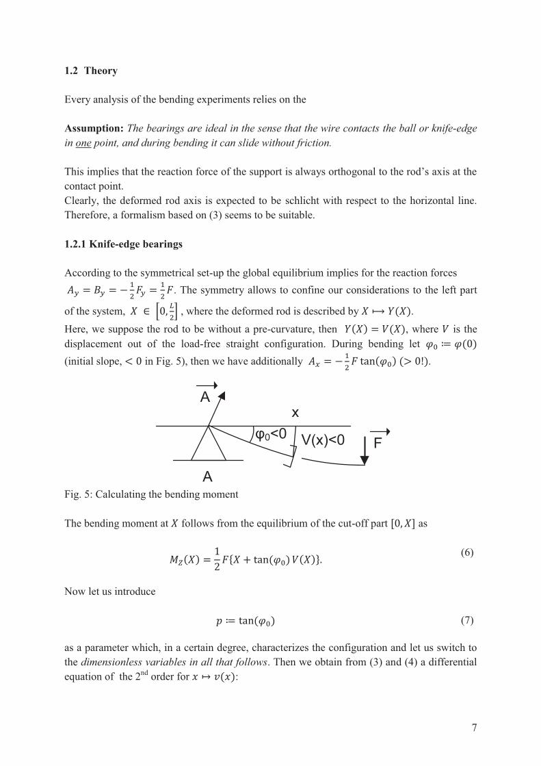
1.2 Theory Every analysis of the bending experiments relies on the Assumption: The bearings are ideal in the sense that the wire contacts the ball or knife-edge in one point, and during bending it can slide without friction. This implies that the reaction force of the support is always orthogonal to the rod’s axis at the contact point. Clearly, the deformed rod axis is expected to be schlicht with respect to the horizontal line. Therefore, a formalism based on (3) seems to be suitable. 1.2.1 Knife-edge bearings According to the symmetrical set-up the global equilibrium implies for the reaction forces . The symmetry allows to confine our considerations to the left part

of the system, , where the deformed rod is described by . Here, we suppose the rod to be without a pre-curvature, then , where is the displacement out of the load-free straight configuration. During bending let (initial slope, in Fig. 5), then we have additionally . Fig. 5: Calculating the bending moment The bending moment at follows from the equilibrium of the cut-off part as

(6)

Now let us introduce

(7) as a parameter which, in a certain degree, characterizes the configuration and let us switch to the dimensionless variables in all that follows. Then we obtain from (3) and (4) a differential equation of the 2nd order for :

F

A

φ0<0 V(x)<0

x

A

8

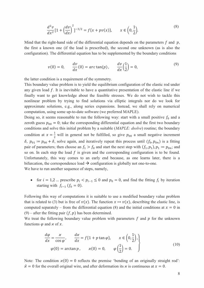
(8)

Mind that the right-hand side of the differential equation depends on the parameters and , the first a known one (if the load is prescribed), the second one unknown (as is also the configuration). The differential equation has to be supplemented by the boundary conditions

(9)

the latter condition is a requirement of the symmetry. This boundary value problem is to yield the equilibrium configuration of the elastic rod under any given load . It is inevitable to have a quantitative presentation of the elastic line if we finally want to get knowledge about the feasible stresses. We do not wish to tackle this nonlinear problem by trying to find solutions via elliptic integrals nor do we look for approximate solutions, e.g., along series expansions. Instead, we shall rely on numerical computation, using some up-to-date software (we preferred MAPLE). Doing so, it seems reasonable to run the following way: start with a small positive and a zeroth guess ; take the corresponding differential equation and the first two boundary conditions and solve this initial problem by a suitable (MAPLE: dsolve) routine; the boundary condition at will in general not be fulfilled, so give a small negative increment

, solve again, and iteratively repeat this process until is a fitting pair of parameters; then choose an and start the next step with ; and so on. In each step the load is given and the corresponding configuration is to be found. Unfortunately, this way comes to an early end because, as one learns later, there is a bifurcation, the correspondence load � configuration is globally not one-to-one. We have to run another sequence of steps, namely,

� for prescribe and and find the fitting by iteration starting with

Following this way of computations it is suitable to use a modified boundary value problem that is related to (3) but is free of . The function , describing the elastic line, is computed separately – from the differential equation (8) and the initial conditions at in (9) – after the fitting pair has been determined. We treat the following boundary value problem with parameters and for the unknown functions and of .

(10)

Note: The condition reflects the premise ‘bending of an originally straight rod’:

for the overall original wire, and after deformation its is continuous at .

9

If is a fitting pair that has been determined by means of (10) through a sequence of iteration steps sketched above, then the corresponding configuration is numerically computed by integrating the initial value problem

(11)

yielding the left half of the elastic line, the right half is then obtained by symmetric continuation. Remark 1 If the test object was a wire of pre-curvature , then the 2nd differential

equation in (10) would change to with the 2nd boundary condition now The boundary value problem (11) would take the form

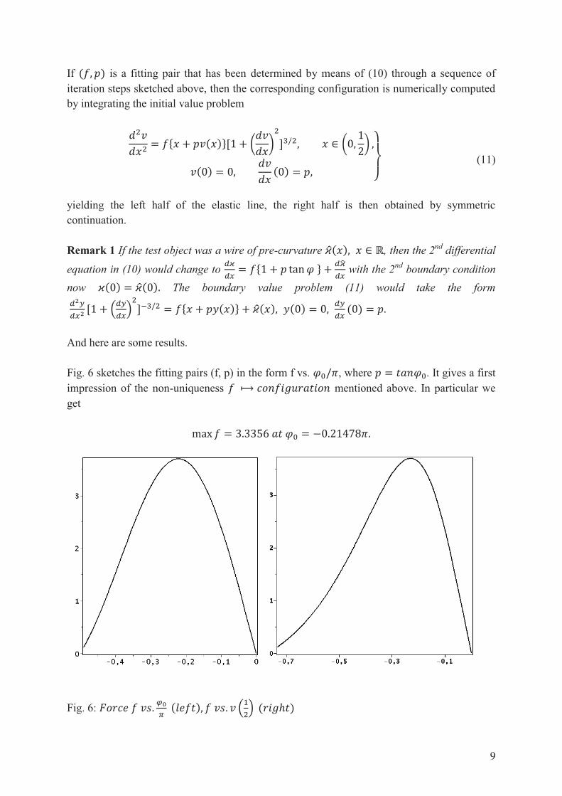
And here are some results. Fig. 6 sketches the fitting pairs (f, p) in the form f vs. , where . It gives a first impression of the non-uniqueness mentioned above. In particular we get

Fig. 6:

10

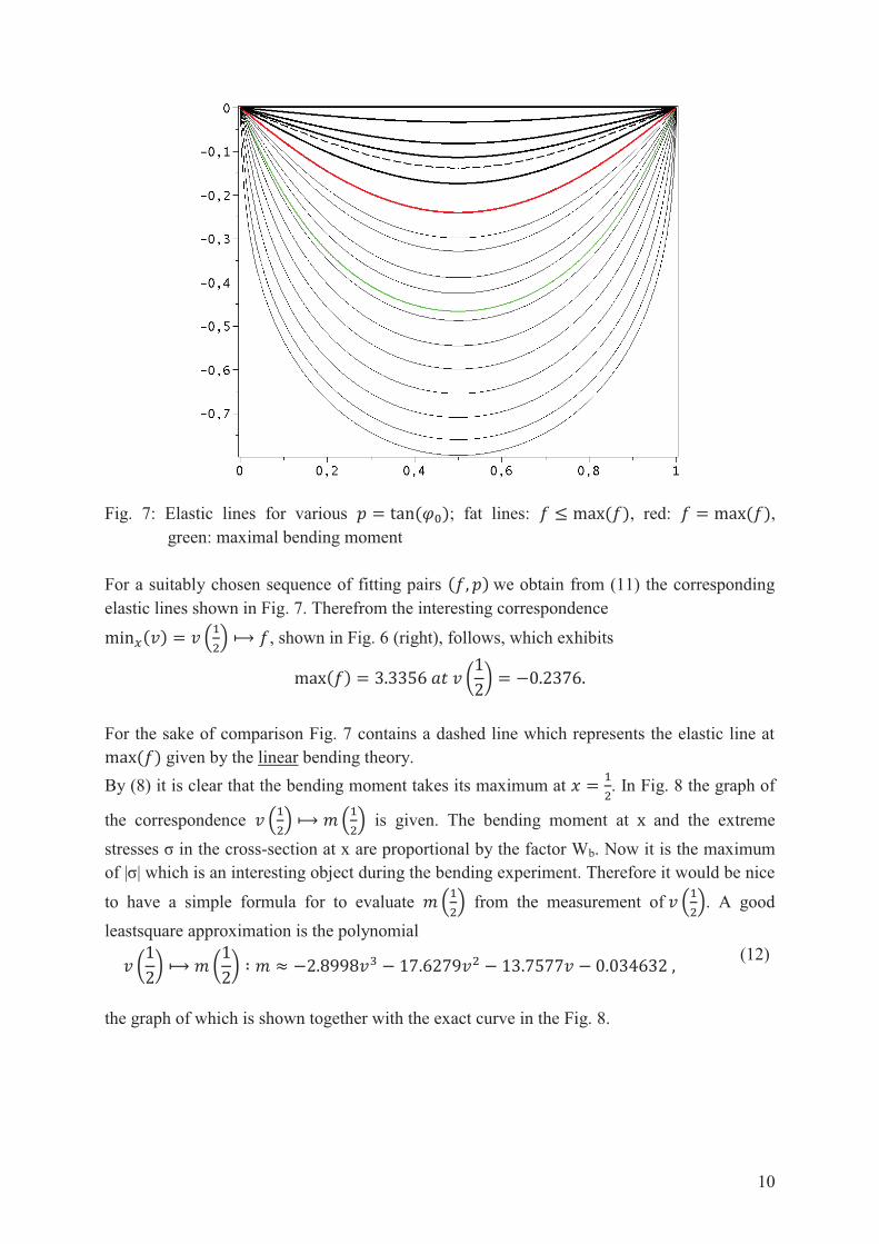
Fig. 7: Elastic lines for various ; fat lines: , red: ,

green: maximal bending moment For a suitably chosen sequence of fitting pairs we obtain from (11) the corresponding elastic lines shown in Fig. 7. Therefrom the interesting correspondence

, shown in Fig. 6 (right), follows, which exhibits

For the sake of comparison Fig. 7 contains a dashed line which represents the elastic line at

given by the linear bending theory. By (8) it is clear that the bending moment takes its maximum at . In Fig. 8 the graph of

the correspondence is given. The bending moment at and the extreme stresses σ in the cross-section at x are proportional by the factor Wb. Now it is the maximum of |σ| which is an interesting object during the bending experiment. Therefore it would be nice

to have a simple formula for to evaluate from the measurement of . A good leastsquare approximation is the polynomial

(12)

the graph of which is shown together with the exact curve in the Fig. 8.

11

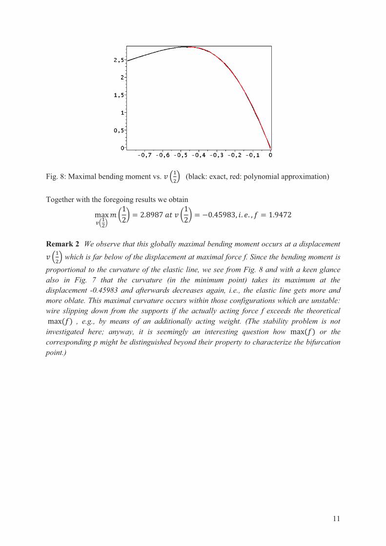
Fig. 8: Maximal bending moment vs. (black: exact, red: polynomial approximation) Together with the foregoing results we obtain

Remark 2 We observe that this globally maximal bending moment occurs at a displacement

which is far below of the displacement at maximal force f. Since the bending moment is proportional to the curvature of the elastic line, we see from Fig. 8 and with a keen glance also in Fig. 7 that the curvature (in the minimum point) takes its maximum at the displacement -0.45983 and afterwards decreases again, i.e., the elastic line gets more and more oblate. This maximal curvature occurs within those configurations which are unstable: wire slipping down from the supports if the actually acting force f exceeds the theoretical

, e.g., by means of an additionally acting weight. (The stability problem is not investigated here; anyway, it is seemingly an interesting question how or the corresponding p might be distinguished beyond their property to characterize the bifurcation point.)

12

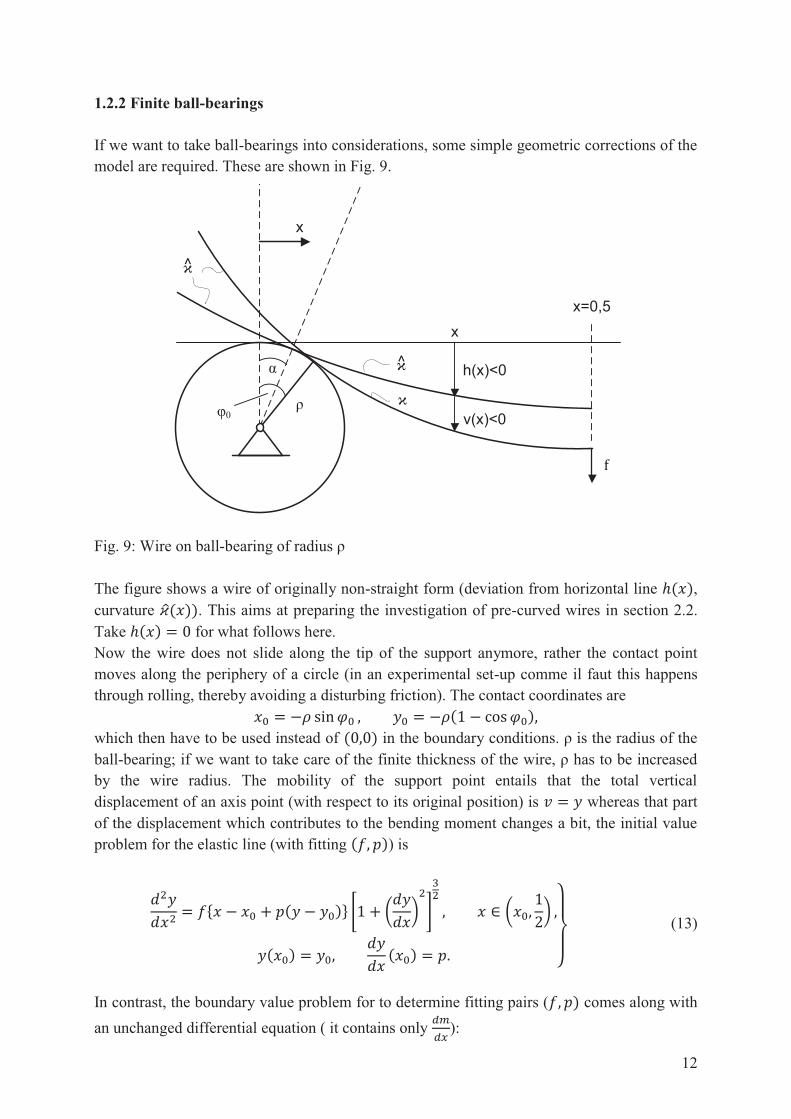
1.2.2 Finite ball-bearings If we want to take ball-bearings into considerations, some simple geometric corrections of the model are required. These are shown in Fig. 9. Fig. 9: Wire on ball-bearing of radius ρ The figure shows a wire of originally non-straight form (deviation from horizontal line , curvature . This aims at preparing the investigation of pre-curved wires in section 2.2. Take for what follows here. Now the wire does not slide along the tip of the support anymore, rather the contact point moves along the periphery of a circle (in an experimental set-up comme il faut this happens through rolling, thereby avoiding a disturbing friction). The contact coordinates are

which then have to be used instead of in the boundary conditions. ρ is the radius of the ball-bearing; if we want to take care of the finite thickness of the wire, ρ has to be increased by the wire radius. The mobility of the support point entails that the total vertical displacement of an axis point (with respect to its original position) is whereas that part of the displacement which contributes to the bending moment changes a bit, the initial value problem for the elastic line (with fitting ) is

(13)

In contrast, the boundary value problem for to determine fitting pairs ( comes along with an unchanged differential equation ( it contains only ):

α

ρφ0

x

h(x)<0

v(x)<0ϰ

xx=0,5

ϰ ^

ϰ ^

13

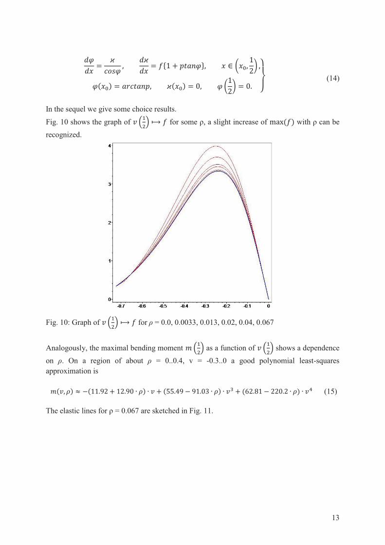
(14)

In the sequel we give some choice results.

Fig. 10 shows the graph of for some ρ, a slight increase of with ρ can be recognized.

Fig. 10: Graph of for ρ = 0.0, 0.0033, 0.013, 0.02, 0.04, 0.067

Analogously, the maximal bending moment as a function of shows a dependence on ρ. On a region of about ρ = 0..0.4, v = -0.3..0 a good polynomial least-squares approximation is

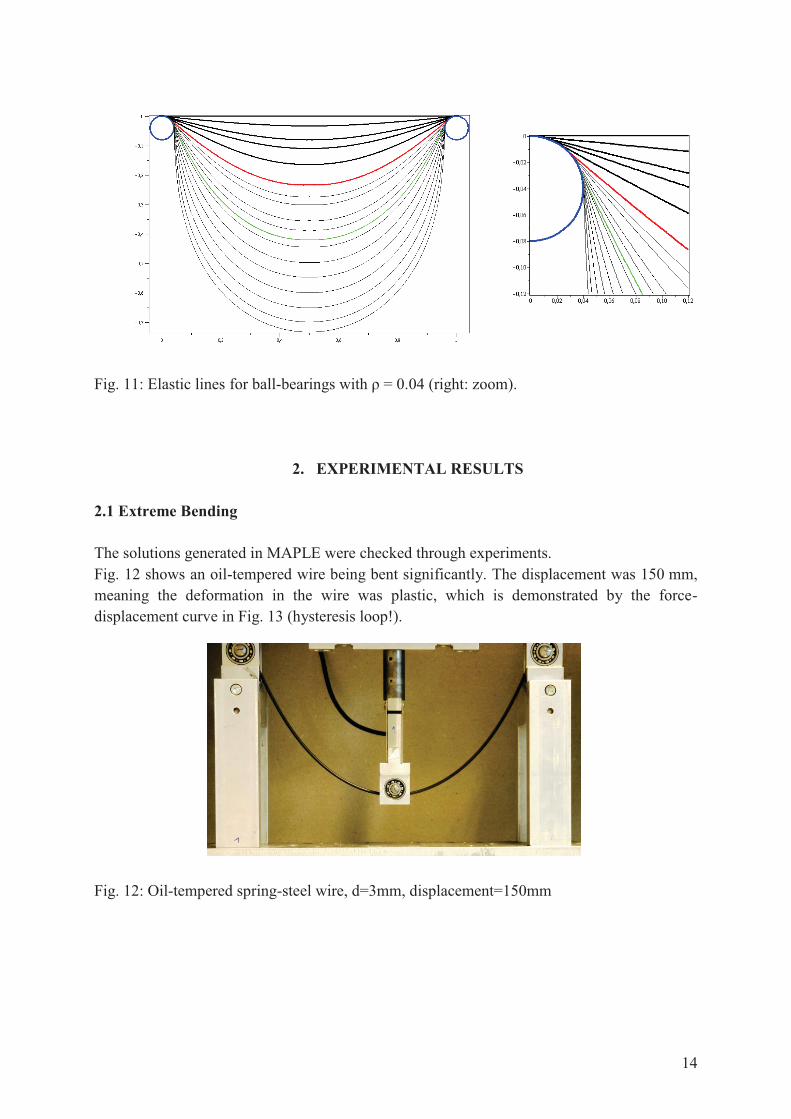
(15) The elastic lines for ρ = 0.067 are sketched in Fig. 11.

14

Fig. 11: Elastic lines for ball-bearings with ρ = 0.04 (right: zoom).

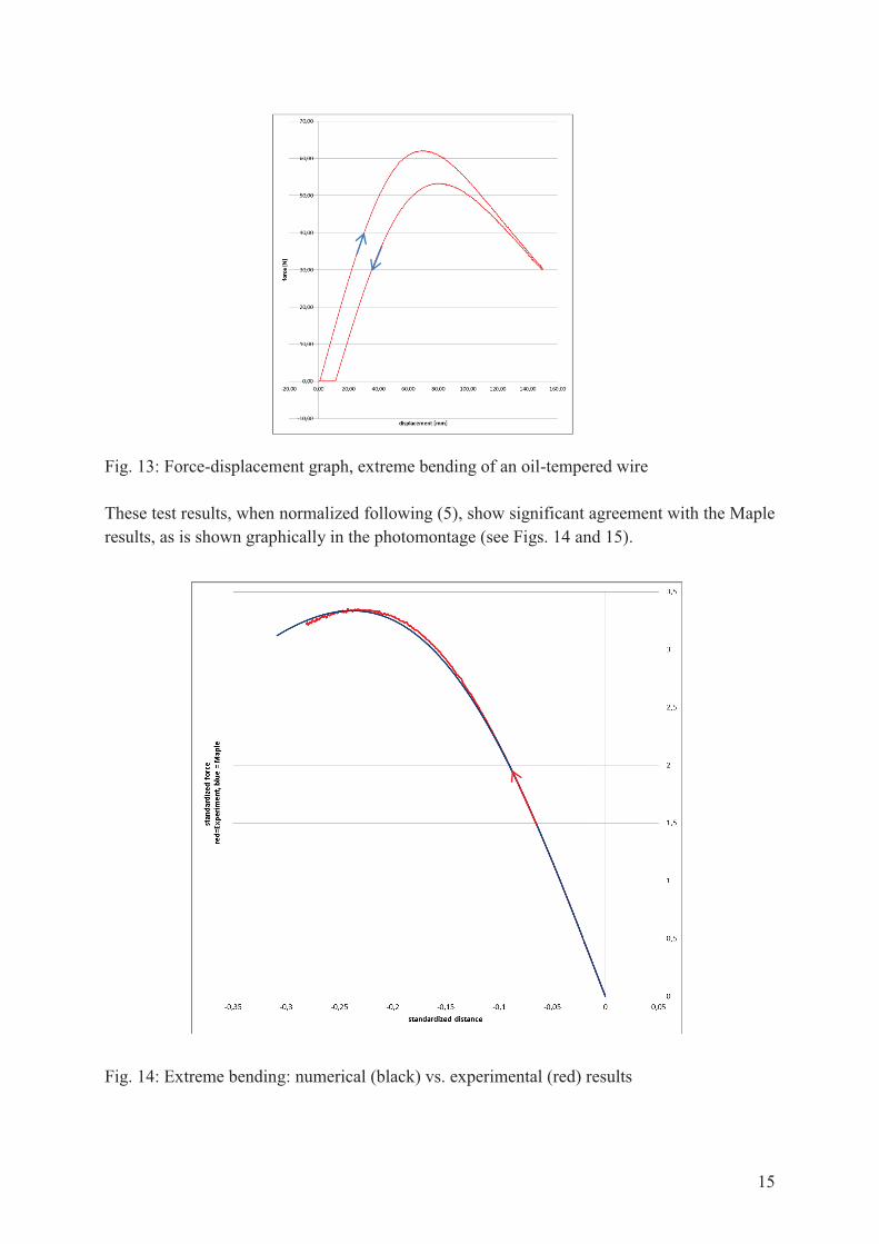
2. EXPERIMENTAL RESULTS 2.1 Extreme Bending The solutions generated in MAPLE were checked through experiments. Fig. 12 shows an oil-tempered wire being bent significantly. The displacement was 150 mm, meaning the deformation in the wire was plastic, which is demonstrated by the force-displacement curve in Fig. 13 (hysteresis loop!). Fig. 12: Oil-tempered spring-steel wire, d=3mm, displacement=150mm

15

Fig. 13: Force-displacement graph, extreme bending of an oil-tempered wire These test results, when normalized following (5), show significant agreement with the Maple results, as is shown graphically in the photomontage (see Figs. 14 and 15). Fig. 14: Extreme bending: numerical (black) vs. experimental (red) results

16

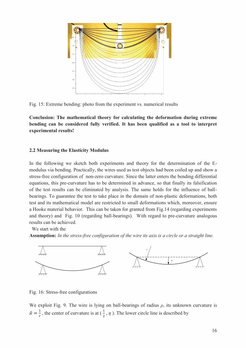
Fig. 15: Extreme bending: photo from the experiment vs. numerical results Conclusion: The mathematical theory for calculating the deformation during extreme bending can be considered fully verified. It has been qualified as a tool to interpret experimental results! 2.2 Measuring the Elasticity Modulus In the following we sketch both experiments and theory for the determination of the E-modulus via bending. Practically, the wires used as test objects had been coiled up and show a stress-free configuration of non-zero curvature. Since the latter enters the bending differential equations, this pre-curvature has to be determined in advance, so that finally its falsification of the test results can be eliminated by analysis. The same holds for the influence of ball-bearings. To guarantee the test to take place in the domain of non-plastic deformations, both test and its mathematical model are restricted to small deformations which, moreover, ensure a Hooke material behavior. This can be taken for granted from Fig.14 (regarding experiments and theory) and Fig. 10 (regarding ball-bearings). With regard to pre-curvature analogous results can be achieved. We start with the Assumption: In the stress-free configuration of the wire its axis is a circle or a straight line.

Fig. 16: Stress-free configurations We exploit Fig. 9. The wire is lying on ball-bearings of radius ρ, its unknown curvature is

, the center of curvature is at ( , η ). The lower circle line is described by

17

and can be measured. From the figure we take

and obtain

Furthermore we have

This completes all we need to apply our differential equations as we did in the foregoing sections. The further progress is as follows.

� Integrating the differential equations we get the displacement in the form with ρ and u as parameters. Then we have

� ρ and u must be measured.

� During the experiments we observe the displacement-force pairs which, following Hooke’s law, are on a straight line, i.e., with slope S to be measured.

� Then (5) entails and finally

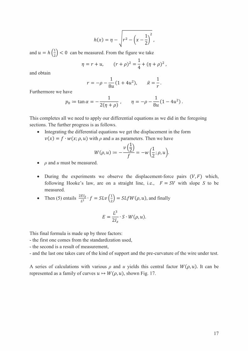
This final formula is made up by three factors: - the first one comes from the standardization used, - the second is a result of measurement, - and the last one takes care of the kind of support and the pre-curvature of the wire under test. A series of calculations with various ρ and u yields this central factor It can be represented as a family of curves , shown Fig. 17.

18

Fig. 17: vs. u for (top to bottom)

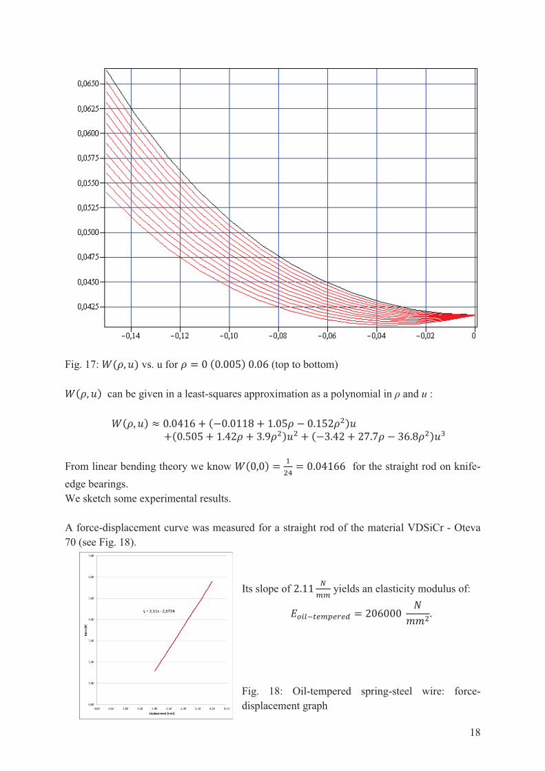
can be given in a least-squares approximation as a polynomial in ρ and u : From linear bending theory we know for the straight rod on knife-edge bearings. We sketch some experimental results. A force-displacement curve was measured for a straight rod of the material VDSiCr - Oteva 70 (see Fig. 18).

Its slope of yields an elasticity modulus of:

Fig. 18: Oil-tempered spring-steel wire: force-displacement graph

19

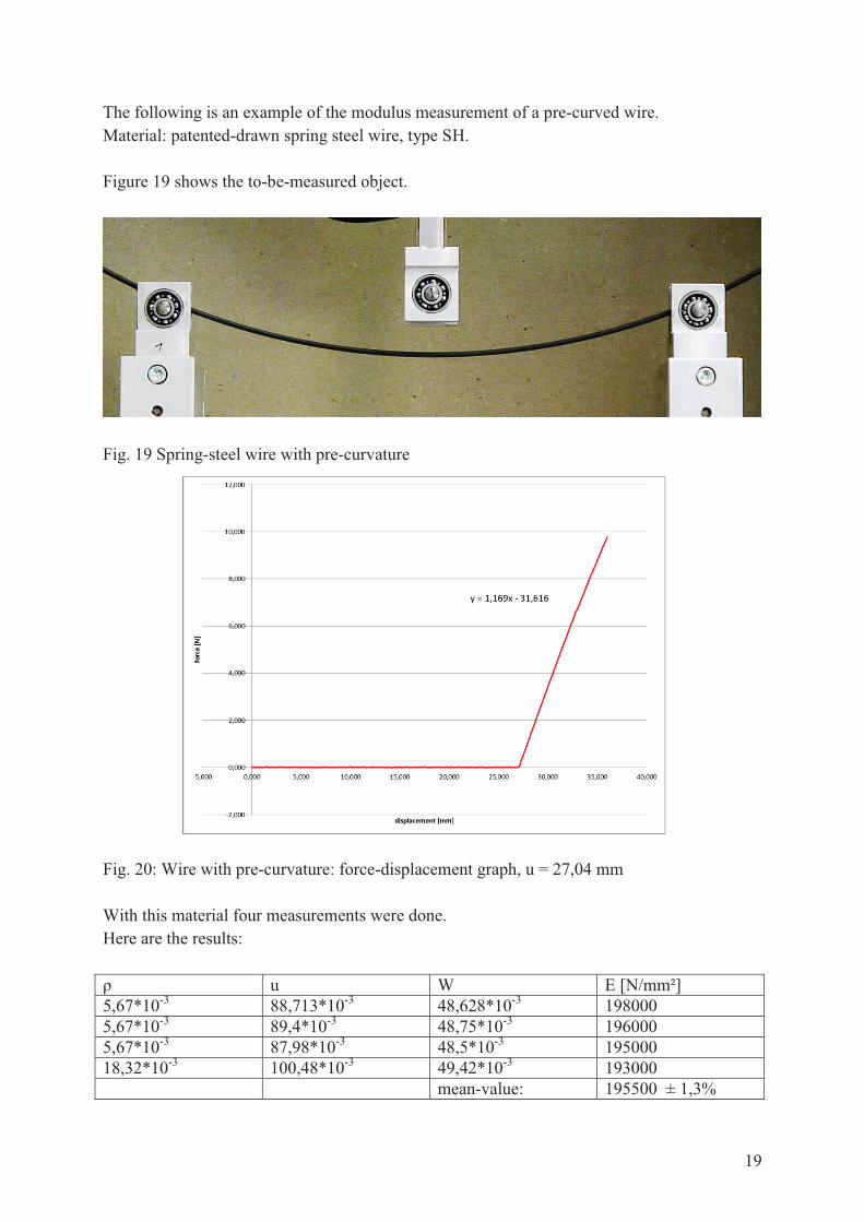
The following is an example of the modulus measurement of a pre-curved wire. Material: patented-drawn spring steel wire, type SH. Figure 19 shows the to-be-measured object.

Fig. 19 Spring-steel wire with pre-curvature Fig. 20: Wire with pre-curvature: force-displacement graph, u = 27,04 mm With this material four measurements were done. Here are the results: ρ u W E [N/mm²] 5,67*10-3 88,713*10-3 48,628*10-3 198000 5,67*10-3 89,4*10-3 48,75*10-3 196000 5,67*10-3 87,98*10-3 48,5*10-3 195000 18,32*10-3 100,48*10-3 49,42*10-3 193000 mean-value: 195500 ± 1,3%

20

2.3 Proposal for Measuring the Spring Bending Limit Industrial applications of flexible springs must ensure that the applied load of the material does not cause plastic deformation. The outer fiber stress, which indicates the limit of permissible elastic deformation, is called the spring bending limit. To experimentally determine the spring bending limit, the standard shown in source [5] (DIN EN 12384) must be kept in mind. The procedure described there is based on a series of

bendings with continuously increasing displacement . When the plastic

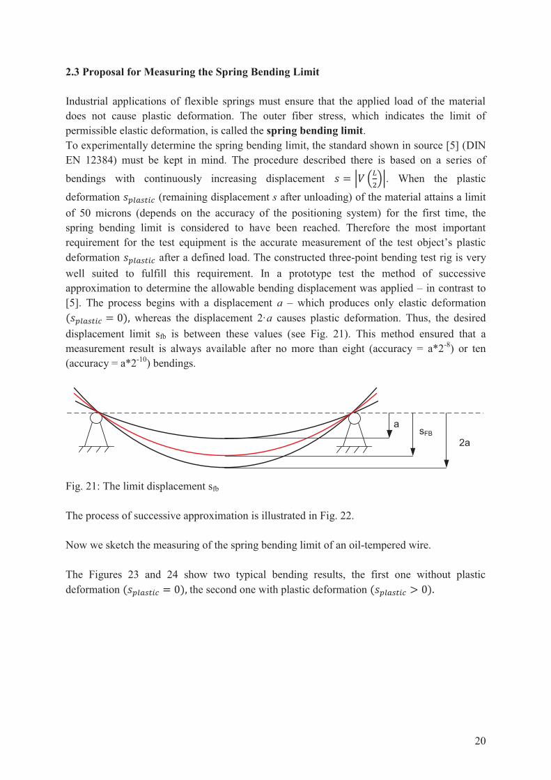
deformation (remaining displacement s after unloading) of the material attains a limit of 50 microns (depends on the accuracy of the positioning system) for the first time, the spring bending limit is considered to have been reached. Therefore the most important requirement for the test equipment is the accurate measurement of the test object’s plastic deformation after a defined load. The constructed three-point bending test rig is very well suited to fulfill this requirement. In a prototype test the method of successive approximation to determine the allowable bending displacement was applied – in contrast to [5]. The process begins with a displacement a – which produces only elastic deformation

whereas the displacement 2·a causes plastic deformation. Thus, the desired displacement limit sfb is between these values (see Fig. 21). This method ensured that a measurement result is always available after no more than eight (accuracy = a*2-8) or ten (accuracy = a*2-10) bendings.

a

2asFB

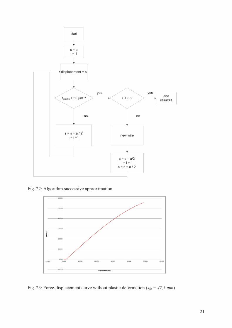
Fig. 21: The limit displacement sfb The process of successive approximation is illustrated in Fig. 22. Now we sketch the measuring of the spring bending limit of an oil-tempered wire. The Figures 23 and 24 show two typical bending results, the first one without plastic deformation the second one with plastic deformation

21

start

s = ai = 1

displacement = s

splastic > 50 µm ?

s = s + a / 2i

i = i +1

i > 8 ?

new wire

s = s – a/2i

i = i + 1s = s + a / 2i

endresult=s

no

yes yes

no

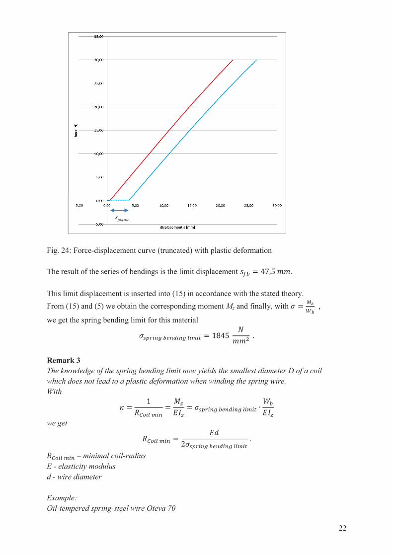
Fig. 22: Algorithm successive approximation Fig. 23: Force-displacement curve without plastic deformation (sfb = 47,5 mm)

22

Fig. 24: Force-displacement curve (truncated) with plastic deformation The result of the series of bendings is the limit displacement This limit displacement is inserted into (15) in accordance with the stated theory. From (15) and (5) we obtain the corresponding moment Mz and finally, with ,

we get the spring bending limit for this material

Remark 3 The knowledge of the spring bending limit now yields the smallest diameter D of a coil which does not lead to a plastic deformation when winding the spring wire. With

we get

– minimal coil-radius E - elasticity modulus d - wire diameter Example: Oil-tempered spring-steel wire Oteva 70

splastic

23

d=3 mm E=206000 N/mm2

Therefore the necessary coil diameter is at least 334 mm. Thus the quotient . Conclusion: The well known formula is correct. With this coil diameter D no plastic deformation of the spring-steel diameter will take place.

3. SUMMARY The paper is a report on recent experimental investigations of spring-steel wires. Spring-steel is a high quality product of the wire industry with outstanding mechanical properties which should ensure that components such as compression springs with smallest mass produce high spring forces. The experimental set-up is a three-point bending test rig. Aim of the experiments was (1) to find the limit of extreme elastic bending of wires – the spring bending limit, and (2) to determine the elasticity modulus of spring-steel via bending thereby using test objects having a pre-curvature. For a quantitative interpretation of the experimental results a suitable mathematical framework is inevitable. To this end an non-linear theory for bending elastic rods is presented. It goes a bit beyond the common mathematical description since different kinds of bearings are considered, and the rods used for the determination of the E-modulus are allowed to be pre-curved. The quantitative mathematical results are gained numerically and afterwards partly presented by handy approximate formulas. Generally, the theoretical considerations are given in a universally utilizable form (use of normalized dimensionless quantities). The experimental set-up and the run of experiments are explained and examples of relevant measuring results are presented. Acknowledgement The authors thank J. Remdt for his careful assistance in executing the experiments.

24

References: [1] Funktions- und fertigungsrelevante Kennwerte für Federstahldraht und Federband IGF-Vorhaben Nr. 16217 BR, TU Ilmenau 2011 [2] Kutschera W.: Elastisches Verhalten dünner Biegefedern konstanten Querschnittes,

Siemens Forschungs-und Entwicklungsberichte Band 7 (1978) Nr.4, Springer Verlag 1978

[3] Sonntag R.: Der beiderseits gestützte, symmetrisch belastete gerade Stab mit endlicher Durchbiegung und seine Stabilität, Ing.-Archiv 12 (1941), S.283-306

[4] Kamke, E., Differentialgleichungen, Lösungsmethoden und Lösungen; Bd.1, Gewöhnliche Differentialgleichungen. Akadem. Verlagsgesellschaft, Leipzig 1944

[5] DIN EN 12384

This research project, ref. no. IGF 16217 BR of the Stahlverformung e.V., has been funded from the budget of the BMWI (the federal German ministry for industry and technology), channelled through a scheme under the aegis of the German Federation of Industrial Research Associations (AiF). It has been actively supported by the Verband der Deutschen Federnindustrie e.V. (Association of german spring producing companies) and its project supervision committee.

Authors: Univ.-Prof. Dr.-Ing. habil. M. Weiß (mathias.weiss@tu-ilmenau.de) Prof. (i.R.) Dr. rer. nat. habil. J. Steigenberger (joachim.steigenberger@tu-ilmenau.de) Dr.-Ing. V. Geinitz (veronika.geinitz@tu-ilmenau.de) Dipl.-Ing. P. Beyer (peter.beyer@tu-ilmenau.de) Ilmenau University of Technology P.O. Box 10 05 65 98684 Ilmenau Germany