Report No. DOT/FAA/RD-94/2

Project Report ATC-208

Extrapolating Storm Location Using the Integrated Terminal Weather System (ITWS)

Storm Motion Algorithm

Lincoln Laboratory MASSACHUSETTS INSTITUTE OF TECHNOLOGY

LEXINGTON, MASSACHUSETTS

Prepared for the Federal Aviation Administration.

Document i11 available to the public through the National Technical Information Service,

Springfield, Virginia 22161.

E. S. Chornoboy A.M. Matlin

29 March 1994

TECHNICAL REPORT STANDARD TITLE PAGE

1. Report No.

ATC-208

4. Title and Subtitle

2. Government Accession No.

DOT/F AAJRD-94/2

3. Recipient's Catalog No.

5. Report Date 29 March 1994

Extrapolating Storm Location Using the Integrated Terminal Weather System (ITWS) Storm Motion Algorithm

6. Performing Organization Code

7. Author(s)

E.S. Chornoboy and A. Matlin

9. Performing Organization Name and Address

Lincoln Laboratory, MIT P.O. Box 73 Lexington, MA 02173-9108

12. Sponsoring Agency Name and Address Department of Transportation Federal Aviation Administration Washington, DC 20591

15. Supplementary Notes

8. Performing Organization Report No.

ATC-208

10. Work Unit No. (TRAIS)

11 . Contract or Grant No.

DTF AO l -9 l-Z-02036

13. Type of Report and Period Covered

Project Report

14. Sponsoring Agency Code

This report is based on studies performed at Lincoln Laboratory, a center for research operated by Massachusetts Institute of Technology. The work was sponsored by the Air Force under Contract Fl9628-90-C-0002.

16. Abstract

Storm Motion (SM) is a planned initial Operational Capability (IOC) algorithm of the FAA's Integrated Terminal Weather System (ITWS). As currently designed, this algorithm will track the movement of storms/cells and convey this tracking information to the ITWS user by means of a graphic display of vectors (for direction) with accompanying numeric reports of storm speed, rounded to the nearest 5 nmi/hr increment. Recognizing that there are occasions when ITWS users could benefit from a more extended product format, Storm Extrapolated Position (SEP) was conceived to supplement the SM product and thereby increase its accessibility as a planning aid.

This communication describes a prototype SEP design along with an analysis of its accuracy and observed performance during 1993 ITWS demonstrations in Orlando (FL) and Dallas (TX).

17. Key Words

Storm Motion Performance Tracking

Extrapolation Correlation

19. Security Class if. (of this report)

Unclassified

18. Distribution Statement

This document is available to the public through the National Technical Information Service, Springfield, VA 22161.

20. Security Classif. (of this page) 21. No. of Pages 22. Price

Unclassified 82

:I> :;o ("') I OS) .p. ._ ________________________________ _.----------------------------------------------------------------co

FORM DOT F 1700.7 (8-72) Reproduction of completed page authorized

-.

ABSTRACT

Storm Motion (SM) is a planned Initial Operational Capability (IOC) algo­rithm of the FAA's Integrated Terminal Weather System (ITWS). As currently designed, this algorithm will track the movement of storms/cells and convey this tracking information to the ITWS user by means of a graphic display of vectors (for direction) with accompanying numeric reports of storm speed, rounded to the nearest 5 mni/hr increment . Recognizing that there are occasions when ITWS users could benefit from a more extended product format, Storm Extrapolated Position (SEP) was conceived to supplement the SM product and thereby increase the latter's accessibility as a planning aid.

This communication describes a prototype SEP design along with an analysis of its accuracy and observed performance during 1993 ITWS demonstrations in Orlando (FL) and Dallas (TX).

iii

--

TABLE OF CONTENTS

Abstract List of illustrations List of Tables

1. INTRODUCTION

1.1 Background 1.2 Motivation 1.3 Report Overview

2. ALGORITHM DESCRIPTION

2.1 Display Concept 2.2 Display Design

3. ALGORITHM PERFORMANCE

3.1 Tracking Accuracy 3.2 Extrapolation Accuracy 3.3 Product Verification 3.4 Nowcast Interpretation

4. CONCLUDING REMARKS

4.1 Report Summary

GLOSSARY

REFERENCES

v

lll

Vll

IX

1

1 1 7

9

9 15

27

27

33 37 51

63

63

69

71

LIST OF ILLUSTRATIONS

Figure No. Page

1 Convective Growth and Storm Motion. 3

2 Advective Storm Motion. 5

3 Storm Motion Display Concept. 9 • 4 Storm Extrapolated Position Display Options. 13

5 Morphologic Closure Filter. 17

6 Defining a Leading-Edge Contour. 17

7 The Storm Extrapolated Po~ition Product I. 21

8 The Storm Extrapolated Position Product II. 23

9 The Storm Extrapolated Position Product III. 25

10 Motion Analysis: Motion Window and Update Rate. 28

11 Fundamental ("Worst Case") Measurement Granularity. 30

12 The Utility of Partially Correlated Measurements. 31

13 Confidence Regions Associated With Extrapolation. 35

14 Extrapolated Position Scoring Format. 37

15 Storm Extrapolated Scoring Comparison I. 39

16 Storm Extrapolated Scoring Comparison II. 41

17 Storm Extrapolated Scoring Comparison III. 43

18 Storm Extrapolated Scoring Comparison IV. 45

19 Storm Extrapolated Scoring Comparison V. 47

20 Storm Extrapolated Scoring Comparison VI. 49

21 Scoring Categories: "Hit" I. 53

22 Scoring Categories: "Hit" II. 53

23 Scoring Categories: "Hit" III. 55

24 Scoring Categories: "Miss By Growth" I. 55

25 Scoring Categories: "Miss By Growth" II. 57

vii

Figure No.

26

27

28

LIST OF ILLUSTRATIONS (Continued)

Scoring Categories: "Miss By Decay" I.

Scoring Categories: "Miss By Decay" II.

Thirty Minute Event Horizon: DFW 4/14/93.

Vlll

Page

57

59

67

Table No.

1

2

3

LIST OF TABLES

Overall Scoring Performance

Performance by Airport

Performance by Average Storm Speed

lX

Page

61

62

62

--

1. INTRODUCTION

1.1 Background

Storm Extrapolated Position (SEP) first appeared during 1993 summer demonstrations as an experimental extension of the Storm Motion (SM) product - the latter a planned component of the Federal Aviation Administration's (FAA) Integrated Terminal Weather System (ITWS). The idea for SEP was born out of an expressed desire by air-traffic controllers and managers for a graphic display that better matched SM to their short-term decision/planning (i.e., timing) needs ("That cell is moving at 40 knots; how much time do we have?"). Specifically, it was suggested that graphic extrapolations of storm location could enhance Storm Motion's usefulness - eliminating the need for controllers to mentally estimate times-of-arrival (TOA) for approaching storms. A rapid development effort by MIT Lincoln Laboratory (LL), combined with useful feedback from controllers and the FAA's Technical Center, resulted in a Storm Extrapolated Position (SEP) product debut during the latter stages of 1993 ITWS demonstrations in Orlando (FL) and Dallas/Fort Worth (TX) .

1.2 Motivation

A storm's "motion" results from the vector sum of cell advection and propagative growth. New cells do not always form in the direction of advection; hence, it is not uncommon for the apparent motion of a multi-cell storm to veer from that of its cellular components ([1]). Figure 1 shows one case observed during 1993 Orlando demonstrations; here, propagative growth represents a significant component of the vector-sum motion. Advection is much easier to track, however, because it manifests as a continuous trend from radar scan to radar scan. Cell growth advances a storm irregularly in bursts; new cells appear at the periphery with a typical frequency of one every 10-20 minutes ([2]; also, note Figure 1).

The LL Storm Motion algorithm ([3]) is built upon a correlation methodology; as such, its tracking ability has proven quite resilient to splitting and merging cells, as well as storm growth and decay. However, the output of this algorithm can only be described as a compromise between reporting both sources of motion vs. reporting advection only. To an extent, this algorithm does track propagative growth; one notable example occurs with the tracking of midwest-type squall lines. More typically, Storm Motion output is dominated by the steady component of cell advection. Because growth manifests as irregular perturbations, its effects are often dampened (even censored) by filters used to ensure a smooth, rather than (wildly) fluctuating, SM behavior. This is particularly evident when there is considerable divergence between growth and advective components, or when new cells appear significantly distant or isolated from the main complex (as in Figures lC and E). In situations such as Figure 1, the Storm Motion output typically reports the cell-advection (exclusive) component (see Figures lA and lD).

It is acknowledged that there is the need for a better indication of growth-induced motion. Unfortunately, there is neither time nor resource to consider growth/decay enhancements for ITWS

1

Initial Operational Capability (IOC) demonstrations; such features can only be phased in as post­IOC upgrades. Given this uncertainty that exists in situations of extreme convective growth, there follows the valid concern that a ubiquitous display of naive storm extrapolations1 has questionable value, especially if users are prone to interpret such extrapolations as nowcasts. This concern is one reason why explicit extrapolation had not been considered previously for IOC.

To date, those who have used the Storm Motion algorithm have not objected to its limitations; in fact, the preliminary feedback has been very favorable. Furthermore, the motivation for SEP per se is user need for TOA information; or, alternatively, an interactive tool with which to query Storm Motion for more detail. As convincing as the negative example of Figure 1 is, there are also many storm environments and situations characterized by long-lived and fast-moving cells ([2, pp. 291-92]). Figure 2 shows an example from the 1993 Dallas/Ft. Worth demonstration; the weather in these frames is more stable and correctly tracked by the SM algorithm.

Given user experience that a storm/cell will continue to exist, what does its observed mo­tion history tell of its impending time of impact? How can this information be provided readily (graphically) without requiring computation on the part of the ITWS user? Putting nowcast inter­pretations aside, could not extrapolations provide this needed timing information, and could they not be implemented for this purpose for IOC? If so, could not proper training and a user's situa­tional awareness then insure that extrapolations were relied on only for timing estimates? Because the above "provisions" seemed sensible, they evoked reconsideration of the extrapolation idea; they underlie the present undertaking of SEP product development.

Surely the ultimate goal is a comprehensive approach uniting motion analysis with growth/ decay detection, trend, and prediction. This cannot be achieved now. However, is it preferable to wait until the technology is fully developed before implementation, or rather is this an opportune prod­uct to employ staged development? There is a valid need that is not serviced by the current Storm Motion algorithm. In the proper context, storm extrapolation represents a feasible and sensible solution. Perhaps equally important, one can argue that introduction of an extrapolated-position product now will provide valuable user experience for phasing growth/decay products in future upgrades.

1The initial concept for an ITWS Geographic Situation Display (GSD), the current working pro­totype, is that of a "dumb" display which can only convey a product's information in all or none fashion; that is, everywhere.

2

'. -

Figure 1. Convective Growth and Storm Motion. This sequence from 1993 Orlando samples with a 10 minute interval and covers a 70 minute period. Cells slowly advect to the south-east; convective growth propagates new cells east. Panel A is the Storm Motion output . Panel D illustrates advection relative to A . In Panels C and E, new cells appear in advance of the complex. Panel H documents the combined effects of advection and growth relative to A. All panels have the same origin and a 1 km pixel size.

3

Figure 2. Advective Storm Motion. This example from 1993 Dallas/ Ft . Worth also cov­ers a 70 minute period. Cells were longer lived and advected considerably fast er than their Orlando counterparts (ref. Figure 1). Panel A shows the Storm Motion output. Panels B through H illustrate the ce ll 's track and show a speed computed using each individual dis­placement . (The lower-right dark-grey area is beyond the radar 's range) . All panels have the same origin and a 1 km pixel size.

5

1.3 Report Overview

This report summarizes initial efforts to design and implement an SEP extension to the ITWS Storm Motion algorithm. Tracking performance is examined and overall performance during 1993 demonstrations is documented, and issues critical to a viable and successful SEP product are identified. The analysis is in part subjective, owing to the time limitations of fast-track product development. Hence, the primary intent of this report is to identify major issues and areas in need of further research/refinement.

The report is organized as follows. Chapter 2 discusses product concept/design and describes the processing steps employed by the 1993 prototype algorithm. Chapter 3 contains a performance analysis of the extrapolated-position product, including observations from 1993 summer demonstra­tions . The first part of Chapter 3 explores limitations related to tracking performance; this analysis is based primarily on previous work with correlation tracking. The second part of Chapter 3 con­tains a "nowcast" analysis of SEP - the point being to underscore the product's limitations in this respect and encourage support for new work in the area of growth/ decay. Chapter 4 concludes the report, summarizing our findings and current recommendations.

7

.T

2. ALGORITHM DESCRIPTION

2.1 Display Concept

Clean and compact formats are required throughout because there will be many ITWS prod­ucts competing for display space, and ITWS users will have but a limited capability to control their display environment. Accordingly, the display concept for the Storm Motion algorithm has been that of unit vectors, for direction, with accompanying storm-speed values in knots (Figure 3A). As a default setting, the product of Figure 3A is believed sufficient to maintain a user 's "situation awareness". However, as implied in the Introduction, recent experience has shown that there are times when a more detailed presentation could have been of value.

Figure 3. Storm Motion Display Concept . A: The Storm Motion algorithm generates vector output with accompanying storm speed in knots; all vectors are drawn with "unit" length . B: Conceptually, a grid having divisions in minutes (and an orientation and spacing that varies with local motion) would be a desirable tool because it translates storm­motion information into useful and accessible timing information. For example, this local grid is oriented in accordance with the motion vectors of Panel A and illustrates the time/ distance relationship using 5 minute increments; the arrow shows where a projected runway impact of 10 minutes is readily inferred from Panel B.

9

Heads-up timing information can aid smooth and efficient change when impending weather events force supervisors to switch among operational modes. For example, Figure 3 incorporates a hypothetical situation where cells traveling northwest at 40-45 knots are expected to impact an airport's runways (parallel red lines). An assumed reconfiguration is about to be scheduled, and there is the need to coordinate this change with the many controlled arrivals and departures. The interval to the time of arrival (TOA) of these cells establishes a frame of reference during which , as a matter of efficiency, it is desired to organize and complete all switches/changes. The product of Figure 3A, however, is not well suited to support such decisions because it burdens the user to compute all desired TOA information, when there are more important matters to attend to. Figure 3B illustrates a (purely) hypothetical display concept wherein an imaginary grid translates local storm-motion information into time-difference ( ~t) intervals , from which TOA values are easily inferred. In many situations there is a need for such a tool - a ruler scaled in divisions of minutes - which can be used to read out ~t intervals.

Figure 4 shows four display options that were considered for Storm Extrapolated Position (SEP). Figure 4A illustrates the simplest - the default storm-motion output is modified such that all vector lengths now correspond to the distance traveled during a fixed elapsed time (10 minutes elapsed time is illustrated). This provides the needed time-scaled metric, but it still requires the user to mentally translate, interpolate, and/or extrapolate vectors to infer the desired ~t information. (We claim it is easier to infer a 10 minute TOA using Figure 3B than it is with Figure 4A.) Figures 4B, C, and D take the critical step and explore variations on the theme of explicit extrapolation. (The options shown are essentially those that were possible given the hardware constraints of the 1993 prototype ITWS display.) In Figure 4B , the solid shape (10 minute extrapolation) obscures too much of the underlying weather (there is no planned hardware capability that would enable translucent shading). The full contours of Figure 4C are an improvement on B, but there would still be the concern that the overlap of multiple contours , such as from multiple extrapolation times, would clutter the display screen. Figures 4B and C are also problematic because they clearly elicit an interpretation as predictions of future precipitation.

Figure 4D is the alternative that was selected for 1993 testing - only the leading edge of a storm is outlined and extrapolated (0, 10, and 20 minutes elapsed time are shown in the figure). Leading-edge contours significantly reduce the display clutter evident with full contours; being a more abstract representation , it can be argued that they discourage interpretations of precipitation

prediction. Features of the advancing envelope front are easily identified, and impact times can be estimated from the "tic marks" provided by 0, 10, and 20 minute edges. The time-0 reference serves to identify a contour with its "parent" cell and also serves as an indicator of product age, since it is unlikely that SEP will be updated as frequently as the underlying precipitation map. The display of Figure 4D also has the advantage of being similar (in form) with other ITWS products that illustrate extrapolated events (i.e., Gust Front); hence, a similarity in interpretation would re-enforce the product's intended use. Once again, in view of current limitations on dealing with storm growth/decay, it is important to emphasize that the SEP product should be viewed only as

11

an attempt to provide the utility of an everywhere-present timing grid - like Figure 3B - but in a compact and non-obtrusive way.

12

.J

Figure 4. Storm Extrapolated Position Display Options. A : Storm Motion vectors have been scaled to show the expected distance that will be traveled in 10 minutes. B: Level-3 shapes can be extrapolated to show estimated locations after 10 minutes (display hardware limitations do not permit translucent shading) . C: Here, extrapolated contours illustrate the expected locations of level-3 cores at 10 and 20 minutes elapsed time. D: Extrapolated leading-edge contours offer the least amount of clutter.

13

2.2 Display Design

The Storm Motion algorithm uses the ITWS Precipitation Product as its input. Hence, the SEP algorithm requires these same data plus the internal motion grid computed by the SM algo­rithm. Extrapolated-position processing is organized upon the following three needs/observations. First, the precipitation product must be processed to improve its "quality" as a source for contours . Second, the algorithm must generate leading-edge contours and include processing to ensure visual continuity and smoothness. Third, contours must be analyzed for relevance, assigned a priority, and packaged for external ITWS display.

The last task above is needed because the current ITWS testbed GSD only permits a product's display in all-or-none fashion. Hence, it is up to the SEP algorithm to choose a small collection of storm contours which it deems representative. Interactive user-selection of contours is more consistent with the product's intent as a tool; algorithm selected contours imply skill with regard to storm-cell significance, which in turn implies predictive capabilities. It is highly recommended that user-selected contours be required ultimately; work is underway to modify the ITWS testbed GSD to permit this functionality.

The experience of 1993 summer demonstrations confirmed that one of the more difficult tasks in developing an SEP product is reliable automated selection and placement of contours. Time limitations prevented any exhaustive research prior to 1993 demonstrations; however, the steps enumerated above - and described more fully below - proved stable and serve as our prototype SEP definition. It should be noted that these steps were defined, implemented, and multiply refined in conjunction with evaluations from controller representatives; this latter interaction took place under the auspices of the FAA's Technical Center.

2.2.1 Shape Smoothing

Morphologic Closure. In 1993, contours were provided only for weather at or above NWS level-3. The observed variations in storm-cell size and an overall rough texture of "raw" precipitation­map contours dictated that some form of smoothing be used to simplify the shapes of SEP. The morphologic filtering method known as "closure" ([4]) was used to link small cells and regions of scattered precipitation and to improve contour smoothness. A 5 x 5 filter window2 and binary morphologic processing were used; the binary threshold was also NWS level-3. Figure 5 illustrates the filter 's use with an example.

2There is a technical issue/problem suggesting further research regarding a "best" morphological filter. This work is not considered critical to current product evaluations and can be examined at a later date.

15

Figure 5. The morphologic operation of "closure " was used to merge and smooth regions before contouring. A : Original precipitation image with final leading-edge contour. B: A 5 x 5 (solid) filter window is used to fill in and connect /eve/-3 and above weather.

Figure 6. A: Leading-edge contours were derived from full (NWS /eve/-3) contours and motion vectors interpolated to the areal centroids. B: A centroid and its motion vector define a rotated coordinate system, which can be used to bisect a full contour into leading and trailing halves. In the Lincoln Laboratory implementation, the leading half was further trimmed to terminate at the points of min and max x'. Steps yet to be completed include checking the local contour slope at each endpoint and sliding-window smoothing.

17

'

2.2.2 Leading-Edge Contours.

Given the morphologically processed precipitation map, contours were generated with the following straightforward approach. Full storm contours were first computed using NWS level-3 as the only threshold. Areal centroids were computed for all full contours and (average) motion vectors for centroids were interpolated from the storm-motion gridded field (Figure 6A). A contour's centroid and the centroid's motion vector define a rotated coordinate system ( x' / y' in Figure 6B), which can be used to bisect a contour into leading and trailing portions. Referring to Figure 6B, "leading-edge" contours were defined as that portion of the front half that ran from the point with minimal x' value to that with maximal x' value. Working inward from these ends, leading-edge contours were "trimmed" (when necessary) until the tangent at the endpoint (local slope) was below a preset threshold. As a final step, each leading-edge contour was smoothed using simple 3-point smoothing.

2.2.3 Quality Checks.

When identifying contour "candidates", two quality checks were applied to remove contours of questionable utility. First, leading-edge contours were eliminated from display if they did not satisfy a minimum-length criterion ( 4 km). Second, contours were eliminated if the motion vector that generated it was found to vary more than 90 degrees from a local neighborhood average. The latter check was a conservative measure taken to block the display of any contour whose motion vector exhibited extreme characteristics (this check should be relaxed in future versions, once additional experience has been obtained). In general, contours were not created if the generating motion vector had a velocity below 5 knots.

2.2.4 Contour Arrangement.

In 1993 it was not possible for the user to selectively "click on" the display of SEP contours as stated, the SEP display was an all-or-none option. For this reason, it was necessary to

select for presentation a subset of the available leading-edge contours. Working with controller representatives, it was agreed that (on average) up to 10 SEP contours could be added to the ITWS GSD without significantly interfering in the display of other products. Therefore, a maximum of 10 displayed SEP contours was adopted. Whenever there were fewer than 10 candidate SEP contours, all were displayed. In the event there were more than 10 candidate contours, prioritization of their

· display was based on radial distance from the airport.

The 3-2-5 Rule. Of greatest interest to controllers are the immediate environs of the airport (0-10 nmi) and the region extending between 30-50 nmi from the airport (specifically, the "goal­posts"). Restricted to the display of a fixed number of contours, these two regions should receive high priority attention. Hence, the following criterion was agreed upon through a collaboration involving the ITWS Controller User Group, which met at the FAA Technical Center in Atlantic City (NJ). Three regions of interest, in order of priority, were defined to be

19

1. '0-10 nmi from the airport,

2. 30-50 nmi from the airport, and

3. 10-30 nmi from the airport.

Within each of these categories, candidate contours were further prioritized by storm speed and contour length. Of the 10 available display "slots", up to 3 were chosen from category (1), 5 from (2), and 2 from (3). If a category could not fill its "quota", additional contours from other categories were added.

2.2.5 Results and Future Refinements

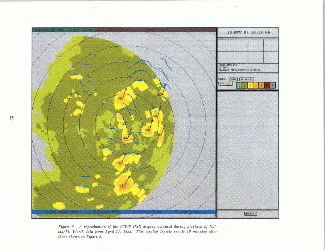
The steps outlined above were found sufficient for most of the situations encountered in Or­lando and Dallas/Ft. Worth. Figure 7 shows an SEP display from the 1993 Orlando demonstration. In general, this display is representative of the development goals that were set and achieved for 1993. There are clear examples where the level-3 grouping described in Section 2.2.1 produced a questionable representation (the elongated storms southeast of the airport). Figures 8 and 9 are examples taken from the 1993 demonstration in Dallas/Ft. Worth. The storms in Orlando, more often than not, were characterized by slow-moving highly-convective situations. In contrast, Fig­ures 8 and 9 show storms with significant motion. On the negative side - even with the number of SEP contours limited to 10 - there is still the propensity for a "busy" display, as evident in these two DFW examples. These figures argue the need that SEP contours should be brought to display one at a time, by user request. It is expexted that this refinement will be available for all ITWS 1994 IOC demonstrations.

20

,

--

21

-.

N:> i;,,;i

''

Figure 8. A reproduction of the ITWS GSD display obtained during playback of Dal­las/Ft. Worth data from April 14, 1993.

~ C1'

Figure 9. A reproduction of the ITWS GSD display obtained during playback of Dal­las/Ft . Worth data from April 14, 1993. This display depicts events 10 minutes after those shown in Figure 8.

t ,

3. ALGORITHM PERFORMANCE

Given that the Storm Extrapolated Position (SEP) algorithm makes no claim to predict, track, or compensate for storm growth/ decay; evaluation of its performance should focus on the intended service of tracking. Since the SEP contours merely reflect the information of the storm-motion vectors, such an analysis can be decomposed into an evaluation of

• storm-motion vector accuracy,

• the applicability of these vectors for extended inference (i.e., extrapolation), and

• the faithful transmission of information by SEP contours.

Although relevant ITWS data were recorded during 1993, time and resource constraints pre­vent the undertaking of any quantitative tracking analysis with that data. Nevertheless, much of the tracking performance can be inferred from a simple sampling model; the previous study [3] validates this model's application to Lincoln Laboratory's (LL) correlation tracker. Model analysis is relied on also to explore limitations in applying storm-motion vectors for extrapolation.

Prior to algorithm demonstrations in Orlando and Dallas/Ft. Worth, faithful representation by SEP contours was verified by humans visually comparing (subjectively scoring) SEP extrapola­tions against actual weather. Such visual comparisons are hampered, of course, in cases of severe storm growth/ decay. Since the distinction between fair representation and corruption by storm growth/decay is sometimes subjective, this invariably rekindles a linking between SEP contours and the prediction of precipitation. This report therefore adds the evaluation of

• SEPs as nowcasts

to the above list. The intent of this last analysis is only to document the severity of growth/decay effects as a known limitation of SEP contours.

3.1 Tracking Accuracy

3.1.1 Data Resolution and Rate

Precipitation-Map Input. The Storm Motion (SM) estimation algorithm has been tailored

to expect Cartesian input, and the source proposed for the ITWS is a precipitation map derived from the airport's own surveillance radar (ASR-9). Alternative input could be provided by resam­pled low-elevation TDWR data (only low-elevation data offer 360° coverage) or available NEXRAD

27

reflectivity products.3 The TDWR, ASR-9, and NEXRAD data suitable for tracking are all charac­terized by a 1 km spatial sampling (pixel size), which imposes a fundamental limitation on motion detection/ estimation. The ASR-9 derived precipitation and the layered (or composite) NEXRAD maps have the distinction and advantage of incorporating vertical "integration", which likely would improve tracking stability (TDWR data at extended ranges would miss precipitation aloft). The TDWR and NEXRAD data are limited to a nominal update rate of 5 minutes; ASR-9 data has the potential for a 30 second update rate. Since time sampling also imposes a fundamental limitation on motion detection and accuracy, ASR-9 data offers (in this respect) the potential for superior tracking performance (see below).

Motion Window. Since time frames compared for motion detection need not appear succes­sively within the sequence, there is a distinction between the interval used for motion detection and the rate at which new images are made available for analysis (ref. Figure 10). The term "motion

••• •••

MOTION WINDOW

UPDATE RATE

Figure 10. Motion estimation requires analysis across a window for detection; the mo­tion window need not be the same as the update rate, which is the rate at which motion measurements are made.

window" is used for the interval between frames that are compared for motion detection. The

3Input from the TDWR (or NEXRAD) could also be used to supplement the ASR-9 data by pro­viding coverage directly over the airport. No such integration existed during 1993 demonstrations, however, and none is planned as an IOC capability.

28

"update rate" , in turn, is the rate at which one can update the sequence of motion estimates. As a first approximation, we consider the implications of sampling a rigid body whose boundaries are (initially) aligned with the sampling grid and whose motion is along one of the principle axes of the grid. In this case, a storm must move at least 1 pixel between comparison frames if motion is to be detected. For all available Cartesian input sources, this implies that storm displacements are generally measured with a 1 km granularity. Figure 11 plots distance moved versus storm speed for three motion windows/intervals and illustrates, by way of staircase plots, the granularity of detected motion. Longer motion windows (10 min) permit finer velocity resolution (by virtue of the greater distance traveled) but incur a higher cost in correlation computations. There is a strong argument against long motion windows: with increasing window size, storm growth/ decay reduces the algorithm's ability to match weather patterns between frames. On the other hand, too short a motion window incurs a high price in quantization error. A preliminary assessment of the trade-off between velocity resolution , computation, and resilience to growth/ decay (conducted at the start of 1993 operations) indicated that a sampling window near 4-5 minutes was required for stable tracking performance with ASR-9 data. This result assumed, however, that the update rate would be the same as the motion window (higher update rates could enable a relaxation to shorter motion windows, but large shifts are considered unlikely). During 1993 summer ITWS demonstra­tions, both motion window size and update rate were set to 5 minutes. A planned upgrade to the tracking algorithm, which is currently underway, is a modification to support the higher update rates possible with ASR-9 data. We note that one further (potential) advantage of the high ASR-9 data rate is that it permits future ITWS extensions to rely on adaptive motion windows , where the window length can be matched to observed storm speed. There are, however , no provisions for an adaptive scheme with the IOC implementation.

3.1.2 Velocity Resolution Model

Quantization Model. With TDWR (or NEXRAD) input, there is a maximum data rate of one precipitation image per 5 minute interval. This update/sampling can be used to define one limit on obtainable accuracy, and since this was also the mode used for all 1993 demonstrations , its associated limitations are relevant to 1993 performance. One can take account of the sampling granularity in estimated storm speed V by modeling V as the sum of a true (continuous) storm speed V plus a quantization error E of the order ±1/2 pixel. To a first approximation, we assume E to be uniformly distributed over the interval (1.852r/60t1 • [-1/2, 1/2]; that is,

where U [ -30 30 ]

€,..., ' 1.852r 1.852r

(1)

(1.852 km = 1 nmi). For a sampling interval r of 5 minutes, this implies a fundamental velocity resolution characterized by the (Equation 1 derived) standard deviation (SD) of ±1.87 nmi/hr. This is a conservative estimate, however, as some spatial and temporal data averaging can be (and is) used to mitigate this limitation.

29

10

-E 8 ~ -c UJ > 6 0 :E UJ 0 4 z t! U>

2 Q

0

- - - - -- - - - -

- - - - - - - - -' - - - - - 5 MIN SAMPLING - - - - - - - -

- - - - -

2.5 MIN SAM PUNG

0 10 20 30 40 50 VELOCITY (nmi/hr)

Figure 11. Fundamental ("Worst Case") Measurement Granularity: Solid-lines plot the relationship D = (1.852/60) V r, where distance D is in km, sampling interval T is in minutes, and velocity V is in nmi/hr. Staircase plots show the corresponding relationship between velocity and "pixels moved", where the image pixel size is 1 km.

Multiple Measurements and Averaging. The tracker uses spatial and temporal averaging to improve velocity-estimation resolution. The capability for spatial averaging is shown in Figure 12, which illustrates how the correlation tracker uses partially correlated measurements to improve tracking performance. Temporal averaging, as discussed in [3], is also used to improve resolution.

Tracking with TDWR or NEXRAD data - which are limited to a 5-minute update rate - one cannot average too far in time without introducing long system lags, sacrificing an adaptability to acceleration (i.e., change of direction). Also, excessive temporal filtering serves to further reduce the influence of growth-induced motion (see Section 1.2, page 1). However, the ASR-9 data rate of one radar image per 30 seconds represents a ten-fold increase relative to TDWR. Inasmuch as these extra data represent independent motion measurements, there is the potential for a significant reduction, by a factor of Jio, in the standard deviation implied by (1). This improvement was not in place for the ITWS demonstration in 1993 but is a planned IOC upgrade. Whether a full "JlO" improvement will be realized must to be verified.

30

Figure 12. The Utility of Partially Correlated Measurements. A: Centroid trackers, and some forms of correlation tracking, identify a storm cell region and track it between time frames; this results in one measurement, subject to fundamental resolution limits. B : The ITWS Storm Motion tracker uses overlapping image subregions, resulting in multiple par­tially correlated measurements. Multiple measurements improve tracker robustness and can mitigate the effects of quantization.

31

Verification of Resolution Model. In [3], storm-motion vector accuracy was characterized in the context of TDWR input. That work is relevant here because it confirms that the quantization model described above does very well in, characterizing the performance of the correlation tracker. To summarize that study in part , 90% of the motion vectors produced by the correlation algorithm exhibited error characteristics well within the above quantization limits (standard deviation on the order of 1 nmi/hr). The remaining 10% of errors fell within the statistical limits of (1). The poorer level of performance was clearly associated with slow-moving storms and algorithm startup (equivalently, transitions from a clear-air radar screen to storms entering from beyond the view horizon). A small percentage of "gross" errors or outliers ( <13) did occur, but there are algorithm improvements planned for ITWS which should reduce this value further. Since the tracker used for 1993 demonstrations sampled the ASR-9 data stream at the TDWR rate (ignoring all intervening data) , the above standard error characterizations were used for the present SEP analysis. It has already been noted that improved performance for ITWS can be expected owing to the higher ASR-9 data rate, which was not used to advantage in 1993.

3.2 Extrapolation Accuracy

The above analyses carry over to extrapolation accuracy. A standard deviation (SD) of 1.87 nmi/hr and an extrapolation time of 10 minutes implies an extrapolation SD of 0.31 nmi (0.58 km). Taking ±2 SDs as the model confidence region, a 10 minute extrapolation implies a confidence-region buffer of ±0.62 nmi (±1.2 km); a 20 minute extrapolation has an implied buffer twice as large, and so forth. Figure 13 illustrates the implications of confidence regions associated with extrapolations: the longer the extrapolation, the more uncertainty as to the storm's extrapolated position.

Depending upon a storm's velocity, confidence regions can overlap and be ambiguous . For example, 10 and 20 minute confidence buffers will overlap for storms moving < 11 nmi/hr; 20 and 30 minute buffers, < 19 nmi/hr; and 30 and 40 minute buffers, < 26 nmi/hr. This implies that upper and lower bounds should be imposed on extrapolation. Below 10 nmi/hr, little is gained from separate 10 and 20 minute extrapolations, and perhaps SEP contours should not be provided at all. Anecdotal evidence has related that extrapolations have not proved very useful for such slow-moving storms.

The increased uncertainty associated with longer extrapolations dictates that an upper limit should be imposed as well. In Orlando and Dallas/Ft Worth, the extrapolation upper bound was governed by a need to minimize the product 's exposure to growth and decay effects. Clearly, many cells persist long enough to validate extrapolations beyond 20 minutes. The current inability to discriminate these cells, however, dictates that extrapolations should be kept in line with shorter life cycles on the order of 20-30 minutes. Should longer extrapolations become feasible with added growth/ decay capabilities, it will be necessary to qualify the uncertainty of longer extrapolations. The promise of improved accuracy with the ASR-9 30-second update rate should help in this regard. Nevertheless, this is an area that requires further investigation. We note that the scoring

33

methods used in Section 3.4 make allowance for a ±1 SD confidence region (±1 km at 20 minutes extrapolation).

34

,'

Figure 13. Confidence Regions Associated With Extrapolation. "Leading edge" contours (see Section 2.2) are used to mark the extrapolated positions of a storm cell. Zero, ten, and twenty minute extrapolations are shown. Each extrapolation is represented by a confidence­region buffer of ±2 standard deviations. These regions assume the baseline configuration of a 1 km resolution map and a 5 minute motion window, but no spatial or temporal smoothing.

35

A B

Reference Time, Reference Time

Storm Motion, and + Extrapolated Positions 10 minutes

c D

Reference Time Reference Time

+ + 15 minutes 20 minutes

Figure 14. Extrapolated Position Scoring Format. A: This panel was used to record the Precipitation Product, Storm Motion Product, and Extrapolated Contour Product for given time . B: The Extrapolated Position Product from Panel A was overlaid with the actual precipitation 10 minutes later. C: A comparison 15 minutes later. D: Twenty minutes later.

3.3 Product Verification

Prior to 1993 demonstrations, human subjective scoring was used to verify the SEP product. The analysis was structured around comparison plots having the format defined in Figure 14. The methodology was to compare SEP contours versus actual weather at the intervals of 10, 15, and 20 minutes after each SEP product update; this preliminary analysis was reviewed also by the FAA's Technical Center. The format shown in Figure 14 was also used for the analysis described in Section 3.4. Figures 15-20 are examples taken from these analyses; they were selected as representative of the situations encountered in 1993.4 The figures are arranged in an order that ranges from ideal- and best-case examples to testing and difficult situations.

Figure 15 is perhaps the simplest of all recorded cases: a single storm complex and one SEP contour group. This is possibly the best example of the SEP objective defined and satisfied. The contour display is compact and representative of the storm's advancing position at 10 and 20

4However, inasmuch as these figures are snapshot evaluations of a product, they" are missing the important element of historical context - that is, the experience of the user prior to the product's display.

37

minutes elapsed time. The growth/decay in this example is closely associated with the body of the complex (or is it that fast-moving storms engulf new cells more quickly?); in any event, this is typical of the performance observed with advancing squall lines (a distinct squall-line performance was alluded to on page 1).

Figure 16 shows one of the better performance examples from 1993 Orlando, where estimated motions greater than 30 knots were seldom observed. The data of 8/15/93 contain some of the faster Orlando storms. There are clear examples of decay occurring to the southwest (the airport is located in the center of the radar scan). However, a number of "markers" can be identified in the reflectivity product from which it can be argued that the motion information (that is, the advection component) is essentially correct. Although the SEP contours provide reasonable motion information for the cell complex NNW of the airport, there are clearly the beginnings of new cell growth west of the airport, which are unaccounted for by the SEP product.

Figure 17 shows one of the better cases recorded during Dallas/Ft. Worth operations. In this particular example, storm speeds ranged between 35 and 40 knots; significant growth and decay takes place during the figure's 20 minute interval as well. It should be noted that, here, SEP contours generally reported the advective component of motion. There are clear examples of new cell growth in advance of SEP contours (the region within 40 km of the airport/image center). However, it is also apparent that at the time of the SEP report, there was considerable evidence regarding the new cells' appearance to warrant user caution. Although some cells decayed considerably during the 20 minute interval, sufficient reflectivity remains to indicate that a faithful representation of the cell's motion was presented.

Figure 18 is more typical of the overall situation encountered in Orlando. There may be little need for an SEP product with such slow-moving air-mass thunderstorms. The cells of Figure 18 move at 10-15 knots, which is near the limit for accurate distinction between 10 and 20 minute extrapolations. However, where cells are stable (even some areas with decay) it can be seen that the SEP contours are representative of the advective motion. The problem is that the SEP product cannot flag regions of convective growth for conservative action (neither can it flag safe regions of nonconvective activity). Very significant, and characteristic of the Orlando summer environment, is such convective activity.

Figure 19 is also from Orlando and shows an extreme example of slow-moving storms and an environment dominated by convective cell growth. In this example, cell growth is near opposite in direction to the indicated advective component; the SEP display is clearly of little use. (It is possible to verify the advective component during this time span.) As the airport is located in the center of the radar image, it would have been, in this case, more operationally significant to have had an understanding of the propagative environment.

38

w co

Figure 15. Storm Extrapolated Scoring Comparison I. Dallas/ Ft. Worth , 6/ 8/ 93 (see Figure 14 for scoring format ; range rings _ qre in units of km).

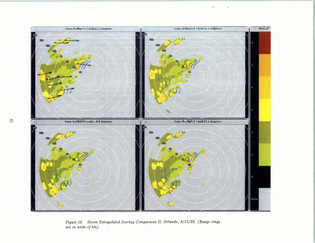
41

.... w

Figure 17. Storm Extrapolated Scoring Comparison III. Dallas/Ft. Worth , 9/13/93. (Range rings are in units of km).

'•

"' oei

."';:: ......,

~

;;:!

"' '-:;

;;:! .;:;>

~

""" <:l

45

~ co

Figure 20. Storm Extrapolated Scoring Comparison VJ. Dallas/Ft. Worth , 4/14/ 93. (Range rings are in units of km).

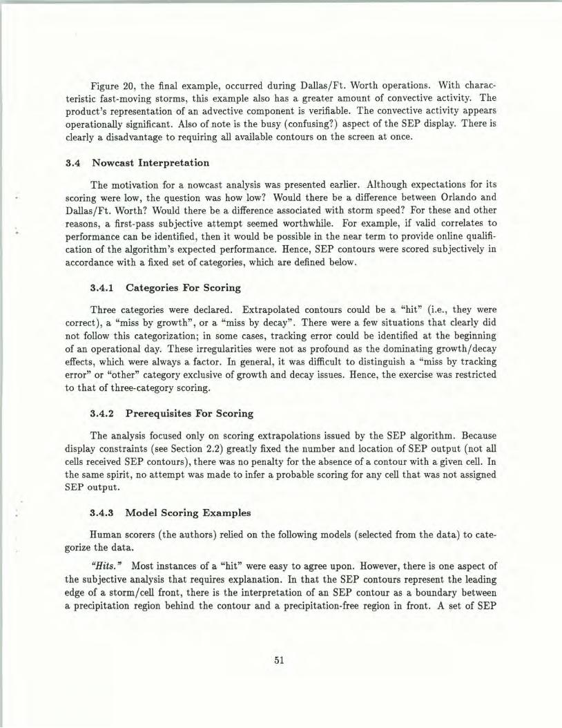
Figure 20, the final example, occurred during Dallas/Ft. Worth operations. With charac­teristic fast-moving storms, this example also has a greater amount of convective activity. The product's representation of an advective component is verifiable. The convective activity appears operationally significant. Also of note is the busy (confusing?) aspect of the SEP display. There is clearly a disadvantage to requiring all available contours on the screen at once.

3.4 Nowcast Interpretation

The motivation for a nowcast analysis was presented earlier. Although expectations for its scoring were low, the question was how low? Would there be a difference between Orlando and Dallas/Ft. Worth? Would there be a difference associated with storm speed? For these and other reasons , a first-pass subjective attempt seemed worthwhile. For example, if valid correlates to performance can be identified, then it would be possible in the near term to provide online qualifi­cation of the algorithm's expected performance. Hence, SEP contours were scored subjectively in accordance with a fixed set of categories , which are defined below.

3.4.1 Categories For Scoring

Three categories were declared. Extrapolated contours could be a "hit" (i.e., they were correct), a "miss by growth" , or a "miss by decay". There were a few situations that clearly did not follow this categorization; in some cases, tracking error could be identified at the beginning of an operational day. These irregularities were not as profound as the dominating growth/ decay effects, which were always a factor. In general, it was difficult to distinguish a "miss by tracking error" or "other" category exclusive of growth and decay issues. Hence , the exercise was restricted to that of three-category scoring.

3.4.2 Prerequisites For Scoring

The analysis focused only on scoring extrapolations issued by the SEP algorithm. Because display constraints (see Section 2.2) greatly fixed the number and location of SEP output (not all cells received SEP contours), there was no penalty for the absence of a contour with a given cell. In the same spirit, no attempt was made to infer a probable scoring for any cell that was not assigned SEP output .

3.4.3 Model Scoring Examples

Human scorers (the authors) relied on the following models (selected from the data) to cate­gorize the data.

"Hits." Most instances of a "hit" were easy to agree upon. However, there is one aspect of the subjective analysis that requires explanation. In that the SEP contours represent the leading edge of a storm/cell front, there is the interpretation of an SEP contour as a boundary between a precipitation region behind the contour and a precipitation-free region in front. A set of SEP

51

contours is regarded as a hit if this interpretation remains valid for each ten- and twenty-minute extrapolation. Variations on this interpretation are covered by the examples of Figures 21-23. Figure 21 illustrates an "ideal" hit. Figures 22 and 23 consider cases where there is storm growth, but the new growth does not violate the spirit of the SEP contour as a "dividing line".

"Miss by growth." Perhaps the most significant type of error is that of new storm devel­opment in advance of the SEP contour "prediction". Figure 24 shows a clear case where new cell growth violates the boundary (between precipitation and clear region) condition of the SEP contour. In many cases, such as that of Figure 24, there is clear evidence of the impending cell appearance. That is, level-1 and level-2 regions in the time-0 panel (ignored by the present SEP algorithm) are present where the new cell appears. A potential direction for future investigation is whether trends in local growth/ decay can be tracked and used to flag potential areas of SEP inapplicability. The example shown in Figure 25 bridges the gap between Hits and Misses. Here, the 10-minute contour alone would be considered a hit. Unfortunately, by 20 minutes elapsed time, growth has just extended beyond the contour to make this a miss.

"Miss by decay." A miss by decay is, in a sense, the opposite of a miss by growth. Specifically, the region in advance of the SEP contours should remain clear for a miss by decay to be declared. Figure 26 illustrates an ideal example of a miss by decay alongside of "hit". A miss by decay represents a case of overwarning and, by virtue of its conservative nature, may be more acceptable than a miss by growth. In many cases, the tracking information is easily verified to have been valid.

52

HITI

Figure 21. Scoring Categories: "Hit" I. This is considered an "ideal" case: level-3 (and above) weather at 10 and 20 minutes is within the confidence regions of the 10 and 20 minute extrapolated contours.

HIT II

Figure 22. Scoring Categories: "Hit" II. Level-3 (and above) weather at 10 and 20 min­utes is within the confidence regions of the 10 and 20 minute extrapolated contours, but new cell growth occurs lateral and behind all contour line extensions. The "dividing­line" interpretation - precipitation behind the contours and a clear region in front - is considered valid.

53

HITlll

Figure 23. Scoring Categories: "Hit" III. There is good agreement between weather and extrapolated contours, but a new cell appears lateral and forward of the contours. The development of the new cell is just beginning; although borderline, th e subjective decision is to score this as a hit.

MISS BY GROWTH I

Figure 24. Scoring Categories: "Miss By Growth " I. New cell growth appears in advance of the SEP contour "predictions". Note, in this case, that there was evidence for the new cells {the level-2 weather), which is ignored by the SEP algorithm.

55

MISS BY GROWTH II

Figure 25. Scoring Categories: "Miss By Growth " II. The growth in this case develops close to the initial complex (the prediction at 10 minutes would be considered a Hit}; new cells at 20 minutes extend beyond the contour, and this is scored as a Miss .

MISS BY DECAY I

Figure 26. Scoring Categories: "Miss By Decay" I. A miss by cell decay is used to describe the specific situation when the weather decays behind the boundary indicated by the SEP contours. The region in advance of the SEP contours remains clear, but the SEP contours, in a sense, now represent an overwarning because regions are becoming clear behind the boundary. At least out to 10 minutes, one can verify that the tracking information is correct.

57

MISS BY DECAY II

Figure 21. Scoring Categories: "Miss By Decay" II. This case is less clear only in the sense that the left-most of these two cells decays to level-2 by 20 minutes elapsed time. As a level-2 cell, it may still be of interest operationally. However, by the scoring criterion defined above, this was declared a Miss . (The cell on the right would be declared a Hit , though). Again, note that the tracking information is essentially correct.

59

3.4.4 Results

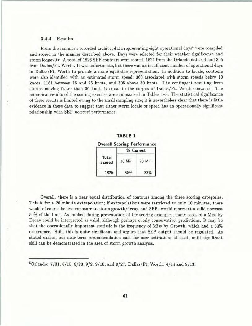
From the summer's recorded archive, data representing eight operational days5 were compiled and scored in the manner described above. Days were selected for their weather significance and storm longevity. A total of 1826 SEP contours were scored, 1521 from the Orlando data set and 305 from Dallas/Ft. Worth. It was unfortunate, but there was an insufficient number of operational days in Dallas/Ft. Worth to provide a more equitable representation. In addition to locale, contours were also identified with an estimated storm speed; 360 associated with storm speeds below 10 knots , 1161 between 15 and 25 knots, and 305 above 30 knots. The contingent resulting from storms moving faster than 30 knots is equal to the corpus of Dallas/Ft. Worth contours. The numerical results of the scoring exercise are summarized in Tables 1-3. The statistical significance of these results is limited owing to the small sampling size; it is nevertheless clear that there is little evidence in these data to suggest that either storm locale or speed has an operationally significant relationship with SEP nowcast performance.

TABLE 1

0 vera II S cormg Pn e ormance

% Correct

Total Scored 10 Min 20 Min

1826 50% 33%

Overall, there is a near equal distribution of contours among the three scoring categories. This is for a 20 minute extrapolation; if extrapolations were restricted to only 10 minutes, there would of course be less exposure to storm growth/ decay, and SEPs would represent a valid nowcast 50% of the time. As implied during presentation of the scoring examples , many cases of a Miss by Decay could be interpreted as valid, although perhaps overly conservative, predictions. It may be that the operationally important statistic is the frequency of Miss by Growth , which had a 33% occurrence. Still, this is quite significant and argues that SEP output should be regulated. As stated earlier, our near-term recommendation calls for user activation; at least , until significant skill can be demonstrated in the area of storm growth analysis.

50rlando: 7 /31, 8/15, 8/23, 9/2, 9/10, and 9/27. Dallas/Ft. Worth: 4/14 and 9/13.

61

TABLE 2

Performance by Airport

% Correct

Total Scored 10 Min 20 Min

DFW

305 60% 37%

MCO

1521 49% 32%

Attempts to isolate performance with respect to locale or storm speed did not alter these results at all. It is true that the fastest storms were exclusive to the Dallas/Ft. Worth region. To the extent that fast storms could be isolated in the Orlando data, there is a slight indication of a trend for scoring improvement with increasing storm speed. It is unclear whether this could be used to any operational advantage. There is at least one correlate that went unexplored. We did not attempt to segregate contours according to average cell life as it was unclear whether this type of statistic could be estimated easily by an unaided algorithm (the ulterior motive is, after all, to identify statistics that can be used to qualify SEP performance online).

TABLE 3

Performance by Average Storm Speed

% Correct

Total Scored 10 Min 20 Min

5-10 knots

360 51% 26%

15-25 knots

1161 48% 34%

> 30 knots

305 60% 37%

62

4. CONCLUDING REMARKS

4.1 Report Summary

In response to controller suggestions, Lincoln Laboratory developed an extrapolated position extension to its Storm Motion (SM) algorithm. In this report, the need for such an extension was interpreted in the context of the controllers' requests, the Storm Motion algorithm's limitations, and the overall structure of Lincoln Laboratory's testbed ITWS system. Given short notice and with scheduled demonstrations in Orlando and Dallas/Ft. Worth fast approaching, the effort to complete this project was intense. Development of the SEP product and its implementation were complete within two month's time, and the algorithm was able to participate in demonstrations in both locales. It should also be noted that a quickly approaching ITWS Demonstration and Validation phase Operational Test and Evaluation (OTE) has likewise limited the time that could be allotted to the present analysis and evaluation. Clearly there are many technical areas in which the product can be improved. This report has ignored them for the most part - choosing instead to focus on an expected SEP capability.

The capabilities of SEP cannot be disassociated from its parent Storm Motion algorithm, and there is a key issue that really should be directed back at that algorithm. Storm Motion has proven itself resilient in the face of growth/ decay, but one should not consider it a faithful predictor of it. Scale is an important factor but the biggest problem is that the Storm Motion algorithm does not have an internal model that allows it to integrate the two very different sources of storm "motion". While a discrete growth component is often detected by Storm Motion's correlation tracker, unless growth occurs for an extended period and in near "steady-state", it is unlikely that the Storm Motion output will sufficiently reflect growth to qualify as a predictor of it. That is why the output product for Storm Motion was conceived as a display of vectors only. The vectors provide direction information and a best (instantaneous) estimate of speed. These quantities were perceived as important components of a display that could provide "quick-look" situation awareness.

The evaluation of the 1993 data confirms the above stated capability of the Storm Motion algorithm. Long-lived cells are faithfully tracked by the motion algorithm, and extrapolations ap­pear to be quite faithful predictions of their future locations - most times surpassing the resolution limitations discussed here. Is advection the primary factor affecting the location of future weather?

The present data suggest that, on average, 20 minute extrapolations would be appropriate pre­dictions only 1/3 of the time. Storm extrapolation does not appear to be an effective nowcast method for the time frame of ATC operations - at least not in Orlando. At an ITWS Controller User Group meeting (held Nov. 16-18, 1993), it was reported that Orlando controllers did not find SEP extrapolations useful in their theater of operations during the summer of 1993. It was also reported, howeve~, that these controllers would reconsider the product given an environment with faster moving storms. In Orlando, storms do move more rapidly in the fall to spring time frame, albeit the frequency of thunderstorms is much less than in the summer.

63

In Orlando, the slow advective component of motion is more often dominated by convective propagation. These slow-moving convective air-mass storms do not test the SEP algorithm in its intended role. The fast moving storms witnessed in Dallas/Ft. Worth suggest that there are environments where advection plays an important role, although the recorded data indicate that growth/ decay is significant there as well. The 1993 Dallas/Ft. Worth data is too sparse to draw any firm conclusions as to whether growth/ decay significantly detracts from the product's e:ffectivenes there.

Figure 28 contains a final example from Dallas/Ft. Worth. On April 14, a plane attempting to land during a storm was unable to hold the runway when it encountered a group of cells sweeping west to east.6 The figure shows four snapshots of the precipitation map; the images are spaced 10 minutes apart and lead to the time of the "incident", which is shown in the final panel. Storm speed during this time was about 40-45 knots (ref. Figure 20). The precipitation map has been highlighted to illustrate a 30 minute event horizon for objects moving at 45 knots. That is, for a cell to reach the airport in Figure 28D - within 30 minutes - it must be within the highlighted region of Figure 28A. In Figure 28A there is clearly little evidence of the cells that become critical in Figure 28D. It is likely that controllers would be more concerned with the cells already over the airport in Figure 28A, and, relying on advection, they might anticipate a temporary clearing if storms continue to advect northeast. Figure 28B shows the beginnings of the new cells, 20 minutes prior to D. In accordance with its 1993 display constraints, however, the SEP algorithm provides a fixed compliment of contours elsewhere (these new cells are small, and the algorithm is incapable of predicting their significance). By Figure 28C, 10 minutes prior to D, the cells have reached a size whereby the SEP algorithm now issues extrapolated positions. The extrapolations are accurate and predict the 10-minute impact time. Because the ITWS demonstration was not operational on this date, we do not know whether this would have been of any help. Regardless, it is our conclusion that extrapolated positions and storm motion will never fully service the type of operational need illustrated here until they become part of a comprehensive treatment that includes storm growth and decay.

The ITWS Controller User Group has indicated a strong desire for products that can be

understood easily - with a quick glance. The scope of the SEP product is to provide this service in the context of tracking cells/storms. The only valid interpretation of SEP supported by the present investigation is that of a tool; that is, a means to an end. In this case the tool takes Storm Motion information and shows, on the GSD screen, what the reported direction and speed mean in units of distance/time. Given its status as a tool, it is preferable for SEP to maintain a lower profile with respect to other displayed (skilled) products. We recommend that there not be a default display of contours, unless governed by an algorithm that is more skilled in anticipating

6The LL testbed was not operational at this time; but ASR-9 and pencil-beam Doppler data were archived, and ITWS products were created afterwards off-line.

64

•

which cells are of interest. We also recommend that the product be brought up by user request, one contour at a time and in response to a user's focused query about a cell/storm.

The SEP product will continue through 1994 and participate in Demonstration and Valida­tion phase OTE operations. Continued experience in the Dallas/Ft. Worth environment, as well as new exposure in Memphis , is considered important for further evaluation. Testbed GSD modifica­tions that will enable SEP display changes in line with the above recommendations are currently underway .

65

•

•

Figure 28. Thirty Minute Event Horizon: DFW 4/ 14/93. Four frames {10 minute sep­aration} of the precipitation product are shown. The average advective motion during this time was 45 knots, moving north east. The DFW airport is indicated by parallel red lines, and the highlighted circular region marks the airport's event horizon with respect to objects moving at 45 knots . About the time of Panel D, an airplane landed just as a cell group , moving east to west, swept the runways - the plane was unable to hold the runway . Panel A shows the situation 30 minutes prior to Panel D: moving at 45 knots, only those cells in the highlighted region can reach the airport within 30 minutes. Panel B shows the precipitation map 20 minutes prior to the incident: there is unclear evidence of the cells that eventually sweep the runway. Panel C shows the precipitation 10 minutes prior to the "incident"; at this time, there is an SEP output that correctly reports an impact in 10 minutes. Panel D is roughly at the time of the incident.

67

,,

•

ASR

ATC

FAA

GSD

ITWS

IOC

LL

NEXRAD

NWS

OTE

SD

SEP

SM

TDWR

TOA

GLOSSARY

Airport Surveillance Radar

Air Traffic Control

Federal Aviation Administration

Geographic Situation Display

Integrated Terminal Weather System

Initial Operational Capability

Lincoln Laboratory

Next Generation Weather Radar

National Weather Service

Operational Test and Evaluation

Standard Deviation

Storm Extrapolated Position

Storm Motion

Terminal Doppler Weather Radar

Time of Arrival

69

REFERENCES

1. K.E. Browning. Morphology and classification of middle-latitude thunderstorms. In E. Kessler, editor, Thunderstorm Morphology and Dynamics, Thunderstorms: A Social, Scientific, and Technological Documentary, chapter 7, pages 133-152. University of Oklahoma Press, Norman, Oklahoma, 1985.

2. C.F. Chappell. Quasi-stationary convective events. In P.S. Ray, editor, Mesoscale Meteo­rology and Forecasting, chapter 13, pages 289-310. American Meteorological Society, Boston, Massachusetts, 1986.

3. E.S. Chornoboy. Storm tracking for TDWR: a correlation algorithm design and evalua­tion. ATC Report ATC-182 (DOT/FAA/NR-91/8), MIT Lincoln Laboratory, Lexington, Mas­sachusetts, 1991.

4. J. Serra. Image Analysis and Mathematical Morphology, Volume I. Academic Press, Inc., San Diego, California, 1982.

71