Extracting Structural InformationUsing Time-Frequency Analysis of Protein NMR Data

Christopher James Langmead∗ Bruce Randall Donald∗ † ‡ §

Abstract

High-throughput, data-directed computational protocols forStructural Genomics (or Proteomics) are required in order toevaluate the protein products of genes for structure and func-tion at rates comparable to current gene-sequencing technol-ogy. To develop such methods, new algorithms are requiredthat can quickly extract significantly more structural infor-mation from sparse experimental data. This paper presents anew class of signal processing algorithms for nuclear mag-netic resonance (NMR) structural biology, based on time-frequency analysis of chemical shift dynamics.

A novel approach to multidimensional NMR analysis isproposed in which the data are interpreted in the time-frequen-cy domain, as opposed to the traditional frequency domain.Time-frequency analysis (TFA) exposes behavior orthogo-nal to the magnetic coherence transfer pathways, thus af-fording new avenues of NMR discovery. An implementa-tion yielding new biophysical results is discussed. In par-ticular, we demonstrate the heretofore unknown presence ofthrough-space inter-atomic distance information within 15N-edited heteronuclear single-quantum coherence (15N HSQC)data. A biophysical model explains these results, and is sup-ported by further experiments on simulated spectra.

1 Introduction

Molecular biology is undergoing a transition towards high-throughput methods. Advances in a variety of different tech-nologies are enabling this transformation. Microarray tech-

∗Dartmouth Computer Science Department, Hanover, NH 03755, USA.†Dartmouth Chemistry Department, Hanover, NH 03755, USA.‡Dartmouth Center for Structural Biology and Computational Chemistry,

Hanover, NH 03755, USA.§Corresponding author: 6211 Sudikoff Laboratory, Dartmouth

Computer Science Department, Hanover, NH 03755, USA. email:brd@cs.dartmouth.edu

Proceedings of The Fifth Annual International Conferenceon Computational Molecular Biology (RECOMB), Mon-treal, April 22-25 (2001) pp. 164-175 .

nology, for example, allows massively parallel high-through-put gene-expression experiments. Consequently, microar-rays have revolutionized modern genetics. Advances in struc-tural genomics methods would enable a similarly radicalchange in structural biology and proteomics. Unfortunately,protein structure determination remains a costly and time-consuming endeavor. Nuclear Magnetic Resonance (NMR)is one of two experimental techniques for determining atomic-resolution structures of biological macromolecules. Stan-dard NMR protocols require running many separate exper-iments. A given experiment can take hours to days of spec-trometer time and it can take weeks to months to prepare aprotein sample needed for a sophisticated experiment (e.g.,residue-specific isotopic labelings). Once the data has beencollected it all must be carefully assigned, analyzed and con-solidated. This process can take months and requires manytedious, manual steps. Due to the many steps in NMR dis-covery, advances in many subproblems are required to de-velop high-throughput methods for NMR structural biology.Automating the manual steps of NMR data assignment andanalysis will be one advance [1-5]. Reducing the amountof spectrometer and wet-lab time by reducing the number ofrequired experiments will be another [1, 2, 6]. Our work fo-cuses on developing new algorithms that can quickly extractsignificantly more structural information from sparse exper-imental data. In this paper, we introduce and analyze a newclass of signal processing algorithms for NMR structural bi-ology, based on time-frequency analysis of chemical shiftdynamics.

Our algorithms leverage the time-varying behavior ofNMR data to extract useful information. This permits thealgorithms to extract more information from NMR data thantraditional methods. In particular, we describe how Time-Frequency Analysis (TFA) can be employed to observe andquantitate Chemical Shift Dynamics (CSD). We demonstratethat CSD can be analyzed using TFA to extract important,and heretofore unobserved structural information, from NMRexperiments. Our algorithm demonstrates the utility of higher-order statistics (in particular, polyspectral analysis and thebicoherence spectrum) for protein NMR, bringing new dataanalysis tools to the armamentarium of the structural biol-

1

ogist. CSD are rich in structural and dynamic information,and yet they have never been previously exploited. TFA al-lows us to decode the information locked in CSD. The CSDTFA protocol effectively defines a new class of NMR experi-ment. Our work shows that the information content of NMRdata (in general) and the 15N HSQC (in particular) is muchhigher than previously believed. Furthermore, since the 15NHSQC is perhaps the simplest, cheapest, and fastest het-eronuclear NMR experiment, our method may have appli-cations in high-throughput structural genomics. We presentthe experimental results of applying our algorithms on twoprotein NMR data sets from (1) human glutaredoxin, whichplays an important role in maintenance of the redox stateof the cell as well as in DNA biosynthesis and (2) core-binding factor, a heterodimeric transcription factor involvedin hematopoesis. Oncogenic translocations in CBF-α and -βare implicated in acute myelomonocytic leukemia.

We now summarize the potential application of our workin high-throughput NMR methods for structural genomics.Generalizing the JIGSAW protocol of Donald and co-workers[1,2], four spectra (the 15N-edited HSQC, 3D 15N-NOESY,80 ms. 15N-TOCSY, and HNHA) from a uniformly 15N-labeled protein would be acquired in a few days. JIGSAW

would then be employed to perform backbone resonance as-signments and calculate secondary structure including β-sheets[1,2]. Next, we wish to constrain and calculate the globalfold in a high-throughput manner. The HSQC can then be re-analyzed (as described in this paper) to reveal correlations inthe CSD TFA 15N-HSQC. CSD TFA yields structural con-straints (distance correlations) that, together with the sec-ondary structure and backbone amide proton assignmentsfrom JIGSAW, can be interpreted as distance restraints tocalculate an approximate global fold. The above set of fourexperiments requires only days of spectrometer time, ratherthan the months required for the traditional suite of dozensof experiments. Furthermore, the proposed protocol only re-quires a protein to be 15N-labeled, a much cheaper and eas-ier process than 13C labeling. From a computational stand-point, we adopt a minimalist approach, demonstrating thelarge amount of information available in a few key spectra.While JIGSAW is used as an example, our method for CSDTFA is actually independent of JIGSAW: alternatively, otherhigh-throughput assignment strategies could be employed[e.g., 3-5], along with secondary structure predictors [e.g.,7, 8] or other NMR methods for rapid secondary structuredetermination [9].

We begin, in Section 2, with a review of the theory andpractice of NMR spectroscopy and discuss the implicationsof protein dynamics on quantum systems. Section 3 detailsour method for extracting time-varying behavior from NMRdata. In section 4 we introduce methods for analyzing time-varying NMR data. Section 5 presents the results of the ap-plication of TFA to the raw HSQC data for human glutare-doxin and CBF-β. Finally, section 6 discusses these resultsand introduces a biophysical model to explain them.

2 NMR Data

Correlations in nuclear spin angular momentum are man-ifested as resonant peaks in NMR spectra. The locationof these peaks in frequency space is measured as chemicalshift. Multidimensional NMR spectra capture interactionsbetween atoms as peaks in R

2 or R3, where the axes indi-

cate resonance frequencies or chemical shifts of atoms. In atypical 15N spectrum peaks correspond to an 15N atom, itsamide proton (HN), and possibly another 1H atom, of par-ticular resonance frequencies. A peak occurs when atomsinteract. Atoms interact via quantum magnetic coherencetransfer either through covalent bonds, or through space.

Traditional NMR structure-determination protocols callfor a number of different experiments. Each experimentgives qualitatively different kinds of information. NMR ex-periments fall into two categories: those (such as NOESY)that transfer magnetization through-space and those (such asHSQC) that transfer magnetization through-bond. Through-space interactions are caused by the Nuclear Overhauser Ef-fect (NOE) which falls off with r−6 [10] and is essentiallyzero beyond 6 Å. Consequently, NOEs are typically em-ployed to derive distance restraints among pairs of protons.Through-bond experiments are used to derive several differ-ent kinds of information, although in general, not distancerestraints. For example, the 15N HSQC is a two-dimensionalthrough-bond experiment correlating the amide proton withthe amide 15N of the same residue [11] (Fig. 1 A). TheHSQC is typically used to determine and pairwise correlatethe chemical shifts of the amide protons and nitrogens alongthe backbone of the protein. These correlations establish theHN-15N connectivities, and the backbone chemical shifts aresubsequently used as reference points within other spectra.

The precise location of an NMR peak in frequency-spaceis determined by a number of factors. Each atom-type hasan inherent chemical shift. For example, in “isolation”, allhydrogen atoms would have the same chemical shift. Thisfundamental frequency is modulated upfield or downfieldvia shielding by the electron clouds and nuclei of nearbyatoms. Within an amino acid (monopeptide), these shield-ing interactions are systematic and repeatable. That is, in atest tube of a given amino acid (e.g., Alanine) in solution,the amide proton for each monopeptide will have the samechemical shift. In a large protein, sequential interactions andthe shielding of atoms brought into spatial proximity due tosecondary and tertiary structure also significantly affect thechemical shift of a given nucleus.

2.1 Chemical Shift Dynamics

Proteins tend to be flexible and in solution, are constantlyundergoing small conformational changes. Since chemicalshifts are affected by tertiary structure [12-14], we must con-clude chemical shifts are in fact dynamic (time-varying). Wewill refer to the phenomena as Chemical Shift Dynamics(CSD).

2

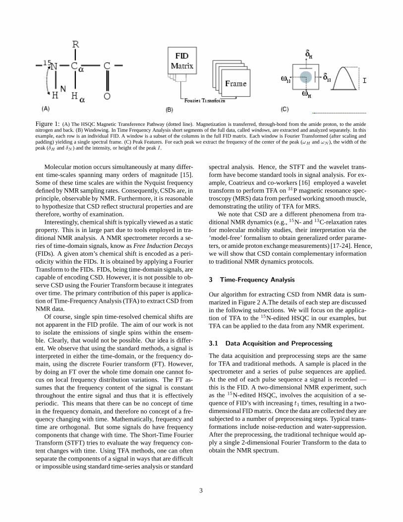
Figure 1: (A) The HSQC Magnetic Transference Pathway (dotted line). Magnetization is transferred, through-bond from the amide proton, to the amidenitrogen and back. (B) Windowing. In Time Frequency Analysis short segments of the full data, called windows, are extracted and analyzed separately. In thisexample, each row is an individual FID. A window is a subset of the columns in the full FID matrix. Each window is Fourier Transformed (after scaling andpadding) yielding a single spectral frame. (C) Peak Features. For each peak we extract the frequency of the center of the peak (ωH and ωN ), the width of thepeak (δH and δN ) and the intensity, or height of the peak I.

Molecular motion occurs simultaneously at many differ-ent time-scales spanning many orders of magnitude [15].Some of these time scales are within the Nyquist frequencydefined by NMR sampling rates. Consequently, CSDs are, inprinciple, observable by NMR. Furthermore, it is reasonableto hypothesize that CSD reflect structural properties and aretherefore, worthy of examination.

Interestingly, chemical shift is typically viewed as a staticproperty. This is in large part due to tools employed in tra-ditional NMR analysis. A NMR spectrometer records a se-ries of time-domain signals, know as Free Induction Decays(FIDs). A given atom’s chemical shift is encoded as a peri-odicity within the FIDs. It is obtained by applying a FourierTransform to the FIDs. FIDs, being time-domain signals, arecapable of encoding CSD. However, it is not possible to ob-serve CSD using the Fourier Transform because it integratesover time. The primary contribution of this paper is applica-tion of Time-Frequency Analysis (TFA) to extract CSD fromNMR data.

Of course, single spin time-resolved chemical shifts arenot apparent in the FID profile. The aim of our work is notto isolate the emissions of single spins within the ensem-ble. Clearly, that would not be possible. Our idea is differ-ent. We observe that using the standard methods, a signal isinterpreted in either the time-domain, or the frequency do-main, using the discrete Fourier transform (FT). However,by doing an FT over the whole time domain one cannot fo-cus on local frequency distribution variations. The FT as-sumes that the frequency content of the signal is constantthroughout the entire signal and thus that it is effectivelyperiodic. This means that there can be no concept of timein the frequency domain, and therefore no concept of a fre-quency changing with time. Mathematically, frequency andtime are orthogonal. But some signals do have frequencycomponents that change with time. The Short-Time FourierTransform (STFT) tries to evaluate the way frequency con-tent changes with time. Using TFA methods, one can oftenseparate the components of a signal in ways that are difficultor impossible using standard time-series analysis or standard

spectral analysis. Hence, the STFT and the wavelet trans-form have become standard tools in signal analysis. For ex-ample, Coatrieux and co-workers [16] employed a wavelettransform to perform TFA on 31P magnetic resonance spec-troscopy (MRS) data from perfused working smooth muscle,demonstrating the utility of TFA for MRS.

We note that CSD are a different phenomena from tra-ditional NMR dynamics (e.g., 15N- and 13C-relaxation ratesfor molecular mobility studies, their interpretation via the’model-free’ formalism to obtain generalized order parame-ters, or amide proton exchange measurements) [17-24]. Hence,we will show that CSD contain complementary informationto traditional NMR dynamics protocols.

3 Time-Frequency Analysis

Our algorithm for extracting CSD from NMR data is sum-marized in Figure 2 A.The details of each step are discussedin the following subsections. We will focus on the applica-tion of TFA to the 15N-edited HSQC in our examples, butTFA can be applied to the data from any NMR experiment.

3.1 Data Acquisition and Preprocessing

The data acquisition and preprocessing steps are the samefor TFA and traditional methods. A sample is placed in thespectrometer and a series of pulse sequences are applied.At the end of each pulse sequence a signal is recorded —this is the FID. A two-dimensional NMR experiment, suchas the 15N-edited HSQC, involves the acquisition of a se-quence of FID’s with increasing t1 times, resulting in a two-dimensional FID matrix. Once the data are collected they aresubjected to a number of preprocessing steps. Typical trans-formations include noise-reduction and water-suppression.After the preprocessing, the traditional technique would ap-ply a single 2-dimensional Fourier Transform to the data toobtain the NMR spectrum.

3

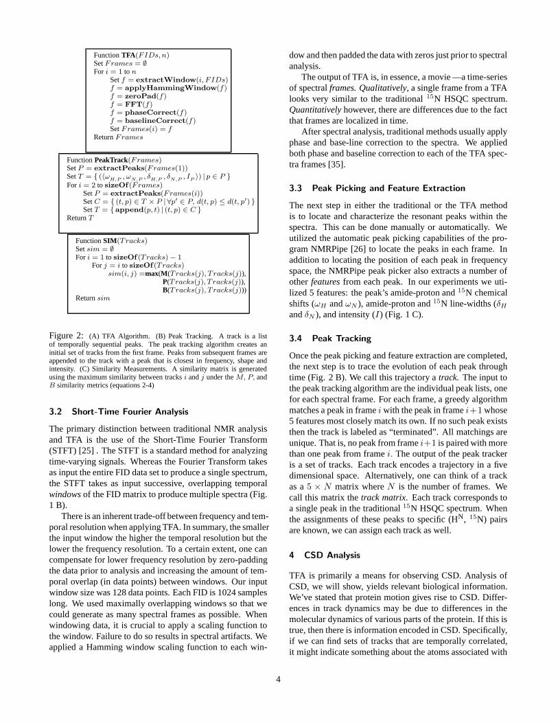
Function TFA(FIDs,n)Set Frames = ∅For i = 1 to n

Set f = extractWindow(i, F IDs)f = applyHammingWindow(f)f = zeroPad(f)f = FFT(f)f = phaseCorrect(f)f = baselineCorrect(f)Set Frames(i) = f

Return Frames

Function PeakTrack(Frames)Set P = extractPeaks(Frames(1))Set T = { (〈ω

H,P, ω

N,P, δ

H,P, δ

N,P, I

P〉) | p ∈ P }

For i = 2 to sizeOf(Frames)Set P = extractPeaks(Frames(i))Set C = { (t, p) ∈ T × P | ∀p′ ∈ P, d(t, p) ≤ d(t, p′) }Set T = { append(p, t) | (t, p) ∈ C }

Return T

Function SIM(Tracks)Set sim = ∅For i = 1 to sizeOf(Tracks)− 1

For j = i to sizeOf(Tracks)sim(i, j) =max(M(Tracks(j), T racks(j)),

P(Tracks(j), T racks(j)),B(Tracks(j), T racks(j)))

Return sim

Figure 2: (A) TFA Algorithm. (B) Peak Tracking. A track is a listof temporally sequential peaks. The peak tracking algorithm creates aninitial set of tracks from the first frame. Peaks from subsequent frames areappended to the track with a peak that is closest in frequency, shape andintensity. (C) Similarity Measurements. A similarity matrix is generatedusing the maximum similarity between tracks i and j under the M, P, andB similarity metrics (equations 2-4)

3.2 Short-Time Fourier Analysis

The primary distinction between traditional NMR analysisand TFA is the use of the Short-Time Fourier Transform(STFT) [25] . The STFT is a standard method for analyzingtime-varying signals. Whereas the Fourier Transform takesas input the entire FID data set to produce a single spectrum,the STFT takes as input successive, overlapping temporalwindows of the FID matrix to produce multiple spectra (Fig.1 B).

There is an inherent trade-off between frequency and tem-poral resolution when applying TFA. In summary, the smallerthe input window the higher the temporal resolution but thelower the frequency resolution. To a certain extent, one cancompensate for lower frequency resolution by zero-paddingthe data prior to analysis and increasing the amount of tem-poral overlap (in data points) between windows. Our inputwindow size was 128 data points. Each FID is 1024 sampleslong. We used maximally overlapping windows so that wecould generate as many spectral frames as possible. Whenwindowing data, it is crucial to apply a scaling function tothe window. Failure to do so results in spectral artifacts. Weapplied a Hamming window scaling function to each win-

dow and then padded the data with zeros just prior to spectralanalysis.

The output of TFA is, in essence, a movie —a time-seriesof spectral frames. Qualitatively, a single frame from a TFAlooks very similar to the traditional 15N HSQC spectrum.Quantitatively however, there are differences due to the factthat frames are localized in time.

After spectral analysis, traditional methods usually applyphase and base-line correction to the spectra. We appliedboth phase and baseline correction to each of the TFA spec-tra frames [35].

3.3 Peak Picking and Feature Extraction

The next step in either the traditional or the TFA methodis to locate and characterize the resonant peaks within thespectra. This can be done manually or automatically. Weutilized the automatic peak picking capabilities of the pro-gram NMRPipe [26] to locate the peaks in each frame. Inaddition to locating the position of each peak in frequencyspace, the NMRPipe peak picker also extracts a number ofother features from each peak. In our experiments we uti-lized 5 features: the peak’s amide-proton and 15N chemicalshifts (ωH and ωN ), amide-proton and 15N line-widths (δH

and δN ), and intensity (I) (Fig. 1 C).

3.4 Peak Tracking

Once the peak picking and feature extraction are completed,the next step is to trace the evolution of each peak throughtime (Fig. 2 B). We call this trajectory a track. The input tothe peak tracking algorithm are the individual peak lists, onefor each spectral frame. For each frame, a greedy algorithmmatches a peak in frame i with the peak in frame i+1 whose5 features most closely match its own. If no such peak existsthen the track is labeled as “terminated”. All matchings areunique. That is, no peak from frame i+1 is paired with morethan one peak from frame i. The output of the peak trackeris a set of tracks. Each track encodes a trajectory in a fivedimensional space. Alternatively, one can think of a trackas a 5 × N matrix where N is the number of frames. Wecall this matrix the track matrix. Each track corresponds toa single peak in the traditional 15N HSQC spectrum. Whenthe assignments of these peaks to specific (HN, 15N) pairsare known, we can assign each track as well.

4 CSD Analysis

TFA is primarily a means for observing CSD. Analysis ofCSD, we will show, yields relevant biological information.We’ve stated that protein motion gives rise to CSD. Differ-ences in track dynamics may be due to differences in themolecular dynamics of various parts of the protein. If this istrue, then there is information encoded in CSD. Specifically,if we can find sets of tracks that are temporally correlated,it might indicate something about the atoms associated with

4

those tracks. For this reason, we chose to explore the notionof similarity among pairs of tracks.

4.1 Track Similarity Measurements

Different similarity measurements emphasize different prop-erties of the tracks. The molecular dynamics which give riseto CSD are varied, complex and typically unknown at thetime of NMR analysis. For these reasons, we implementedthree different track similarity measurements, each target-ing a different kind of information [Fig. 2 C]. It is worthintroducing and reviewing these metrics, since their applica-tion may be unfamiliar in this context. The use of the powerspectrum to infer structural constraints from energetic sim-ilarity in chemical shift dynamics is novel. Our third sim-ilarity metric employs higher-order statistics (specificallypolyspectral analysis and the bicoherence spectrum) [27]which have not been previously applied to any form of bio-polymer NMR.

The first measurement, M , compares track morphologyusing the correlation coefficient. The second measurement,P , compares periodicities within the tracks using the powerspectrum. The power spectrum of a signal is the square ofthe magnitude of its Fourier transform. It reveals the amountof energy present as a function of frequency. Two tracksexperiencing similar periodicities will have similar powerspectra. The final measurement, B, compares nonlineari-ties within the tracks using the bicoherence spectrum [27].The bispectrum is a higher order statistic capable of detect-ing third-order correlations within a signal. It is often usedto detect quadratic phase coupling, a specific type of non-linearity. It is defined as B(ω1, ω2) = Y (ω1)Y (ω2)Y

∗(ω1+ω2) where Y (ω) is the Fourier transform and Y ∗(ω) is itscomplex conjugate. The functions governing CSD are non-linear. Thus, it is possible that tracks will exhibit quadraticphase coupling. Two tracks that are caused or modulated bythe same non-linear process will have similar bispectra. Thebicoherence is the normalized bispectrum. It is defined as

Bc(ω1, ω2) =Y (ω1)Y (ω2)Y

∗(ω1 + ω2)√

|Y (ω1)Y (ω2)|2|Y ∗(ω1 + ω2)|

2

(1)

The bispectrum has previously been utilized in a number ofdomains to extract information from the higher-order statis-tics of natural data [e.g., 27, 28].

We say that two tracks are correlated if their similaritiesexceed a chosen threshold under any of the three similaritymeasurements, otherwise they are uncorrelated. Let C de-note the set of pairs of correlated tracks and let U denote theset of pairs of uncorrelated tracks. C and U are disjoint andthe set C ∪ U is the set of all pairs of tracks. Note that thecardinality of C, and consequently U , is determined by thechosen threshold.

Prior to calculating similarities between pairs of tracks,each profile is normalized to the range [−1, 1]. The similar-

ity between two tracks are only computed over temporallycoincident frames. The M , P , and B similarity measure-ments are calculated as follows. Let X and Y be two trackmatrices. Let xωH

, xωN, xδH

, xδHand xI denote the rows

of X , corresponding to the chemical shift, line-widths andintensity profiles of X , respectively. Note that xωH

, for ex-ample, is a vector of N ωH-values, one for each frame.

Our M similarity measurement is defined as

M(X, Y ) = (r(xωH, yωH

), r(xωN, yωN

), (2)

r(xδH, yδH

), r(xδN, yδN

),

r(xI , yI))

where r(x, y) is the correlation coefficient of vectors x andy.

Our P similarity measurement is defined as

P (X, Y ) = (r(H(xωH), H(yωH

)), r(H(xωN), H(yωN

), (3)

r(H(xδH), H(yδH

)), r(H(xδN), H(yδN

)),

r(H(xI ), H(yI)))

where H (x) is the power spectrum of the vector x, andr(H1, H2) is the correlation coefficient of the power spec-tra H1 and H2.

Our B similarity measurement is defined as

B(X, Y ) = (r(Bc(xωH), Bc(yωH

)), r(Bc(xωN), Bc(yωN

)), (4)

r(Bc(xδH), Bc(yδH

)), r(Bc(xδN), Bc(yδN

)),

r(Bc(xI), Bc(yI)))

where Bc(x) is the bicoherence of the vector x, andr(Bc1, Bc2) is the correlation coefficient of the bicoherencesBc1 and Bc2.

The similarity measurements are in the range [−1, 1].Each similarity measurement (M , P , B) is multidimensional(one dimension per feature) and a separate threshold was se-lected for each dimension. The master threshold for a givensimilarity measurement is adjusted by maintaining the rela-tive positions of the thresholds for the individual dimensions.The global similarity measurement takes the maximum sim-ilarity under M , P and B. The correlated pairs from each ofM , P and B are combined to create the the final, correlatedset. We are presently exploring analytical methods for deter-mining thresholds based on the distributions of similaritiesobserved under a given measurement/dimension.

5 Results

Our technique has been applied to the raw, two-dimensional15N HSQC FID matrices from the two proteins Human Glu-taredoxin (huGrx) [29,30] (PDB ID 1jhb) and Core Bind-ing Factor Beta (CBF-β) [31, 32] (BMRB Accession 4092;

5

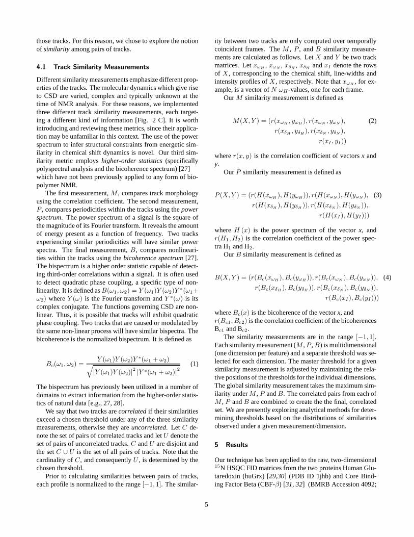
(A) Track Statistics

Protein

CBF-β(ppm) huGrx (ppm) scTCR (ppm)

Mean ∆ Chem. Shift 0.16 0.17 0.27

Max ∆ Chem. Shift 0.78 0.63 0.59

Min ∆ Chem. Shift 0.07 0.07 0.14

St. Dev. ∆ Chem Shift 0.09 0.07 0.09

(B) Inter Atomic Distance Statistics

huGrx CBF-β scTCR

C (Å) U (Å) C (Å) U (Å) C (Å) U (Å)

Mean 11.02 17.07 11.90 22.26 21.23 26.58

Median 9.59 16.56 12.09 21.34 17.37 26.58

Max 23.45 40.76 21.27 53.68 48.00 56.95

Min 3.45 1.85 1.91 1.80 5.20 2.29

Pairs 23 8187 21 19001 21 17780

t-test p < 1.8 × 10−5 p < 7.6 × 10−7 p < 1.9 × 10−2

Table 1: (A) Summary of track statistics for CBF-β, huGrx and scTCR(preliminary results). ∆ chemical shift is calculated as the difference be-tween the highest and lowest proton chemical shift value in each track. (B)Inter-atomic distance statistics for the distribution of temporally correlatedpeaks (C) vs. uncorrelated peaks (U ) in huGrx, CBF-β, and scTCR (pre-liminary results). The number of pairs of protons in each distribution is alsoreported. Student’s t-test confidence scores (p-values) reflect the probabil-ity the differences in means are due to chance.

PDB ID 2jhb). The sizes of the the two proteins are 106and 143 residues respectively. We were provided the original15N HSQC FID data, signal processing parameters, and orig-inal peak lists for each protein by Dr. John Bushweller. 15NHSQC spectra were recorded at Dartmouth on a 500 MHzVarian UnityPlus spectrometer with an actively shielded gra-dient triple resonance probe and pulsed field gradients at20◦C and at 30◦C for CBF-β and huGrx, respectively, in 5%D2O. In our experiments we utilized signal processing pa-rameters similar or identical to those used in [29, 31] whenpossible.

5.1 Observability of CSD

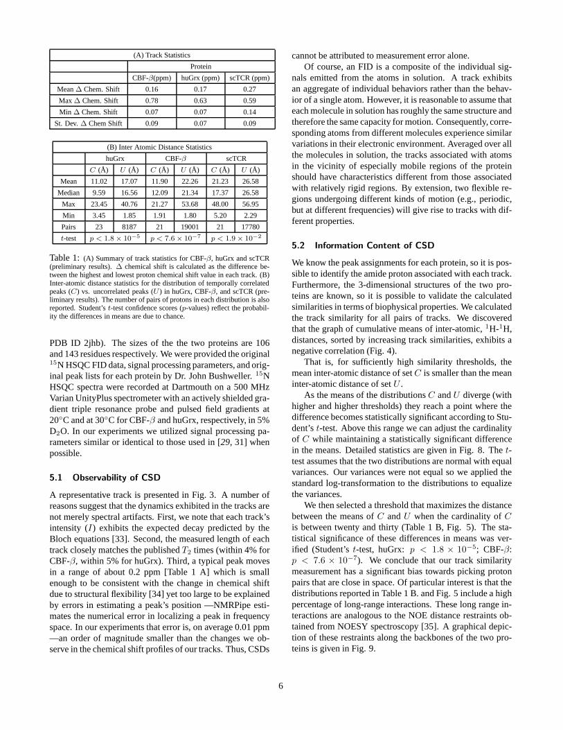
A representative track is presented in Fig. 3. A number ofreasons suggest that the dynamics exhibited in the tracks arenot merely spectral artifacts. First, we note that each track’sintensity (I) exhibits the expected decay predicted by theBloch equations [33]. Second, the measured length of eachtrack closely matches the published T2 times (within 4% forCBF-β, within 5% for huGrx). Third, a typical peak movesin a range of about 0.2 ppm [Table 1 A] which is smallenough to be consistent with the change in chemical shiftdue to structural flexibility [34] yet too large to be explainedby errors in estimating a peak’s position —NMRPipe esti-mates the numerical error in localizing a peak in frequencyspace. In our experiments that error is, on average 0.01 ppm—an order of magnitude smaller than the changes we ob-serve in the chemical shift profiles of our tracks. Thus, CSDs

cannot be attributed to measurement error alone.Of course, an FID is a composite of the individual sig-

nals emitted from the atoms in solution. A track exhibitsan aggregate of individual behaviors rather than the behav-ior of a single atom. However, it is reasonable to assume thateach molecule in solution has roughly the same structure andtherefore the same capacity for motion. Consequently, corre-sponding atoms from different molecules experience similarvariations in their electronic environment. Averaged over allthe molecules in solution, the tracks associated with atomsin the vicinity of especially mobile regions of the proteinshould have characteristics different from those associatedwith relatively rigid regions. By extension, two flexible re-gions undergoing different kinds of motion (e.g., periodic,but at different frequencies) will give rise to tracks with dif-ferent properties.

5.2 Information Content of CSD

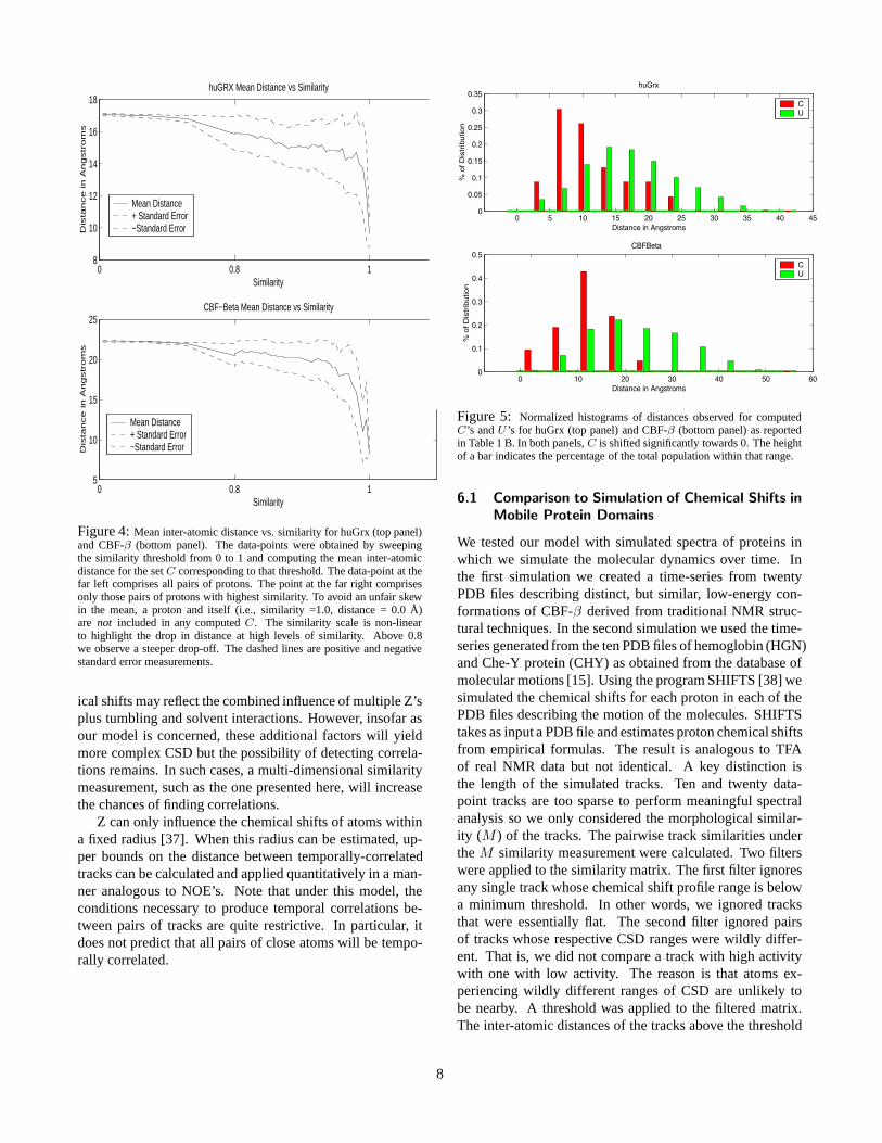
We know the peak assignments for each protein, so it is pos-sible to identify the amide proton associated with each track.Furthermore, the 3-dimensional structures of the two pro-teins are known, so it is possible to validate the calculatedsimilarities in terms of biophysical properties. We calculatedthe track similarity for all pairs of tracks. We discoveredthat the graph of cumulative means of inter-atomic, 1H-1H,distances, sorted by increasing track similarities, exhibits anegative correlation (Fig. 4).

That is, for sufficiently high similarity thresholds, themean inter-atomic distance of set C is smaller than the meaninter-atomic distance of set U .

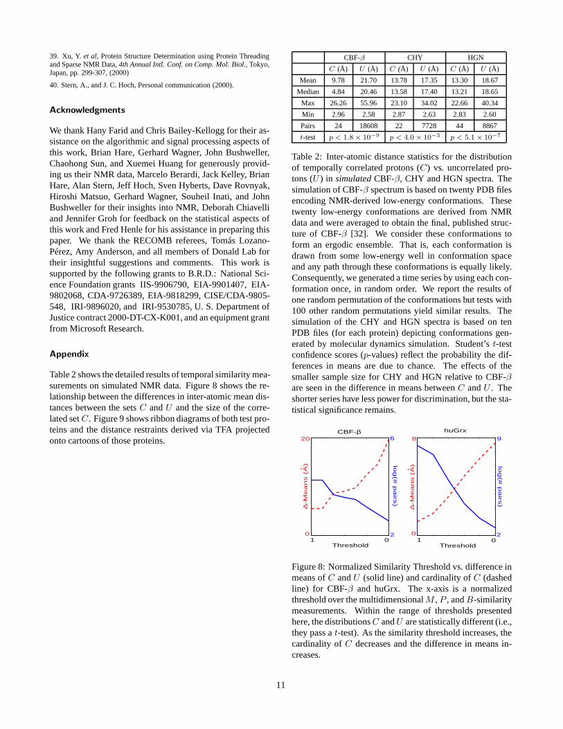
As the means of the distributions C and U diverge (withhigher and higher thresholds) they reach a point where thedifference becomes statistically significant according to Stu-dent’s t-test. Above this range we can adjust the cardinalityof C while maintaining a statistically significant differencein the means. Detailed statistics are given in Fig. 8. The t-test assumes that the two distributions are normal with equalvariances. Our variances were not equal so we applied thestandard log-transformation to the distributions to equalizethe variances.

We then selected a threshold that maximizes the distancebetween the means of C and U when the cardinality of C

is between twenty and thirty (Table 1 B, Fig. 5). The sta-tistical significance of these differences in means was ver-ified (Student’s t-test, huGrx: p < 1.8 × 10−5; CBF-β:p < 7.6 × 10−7). We conclude that our track similaritymeasurement has a significant bias towards picking protonpairs that are close in space. Of particular interest is that thedistributions reported in Table 1 B. and Fig. 5 include a highpercentage of long-range interactions. These long range in-teractions are analogous to the NOE distance restraints ob-tained from NOESY spectroscopy [35]. A graphical depic-tion of these restraints along the backbones of the two pro-teins is given in Fig. 9.

6

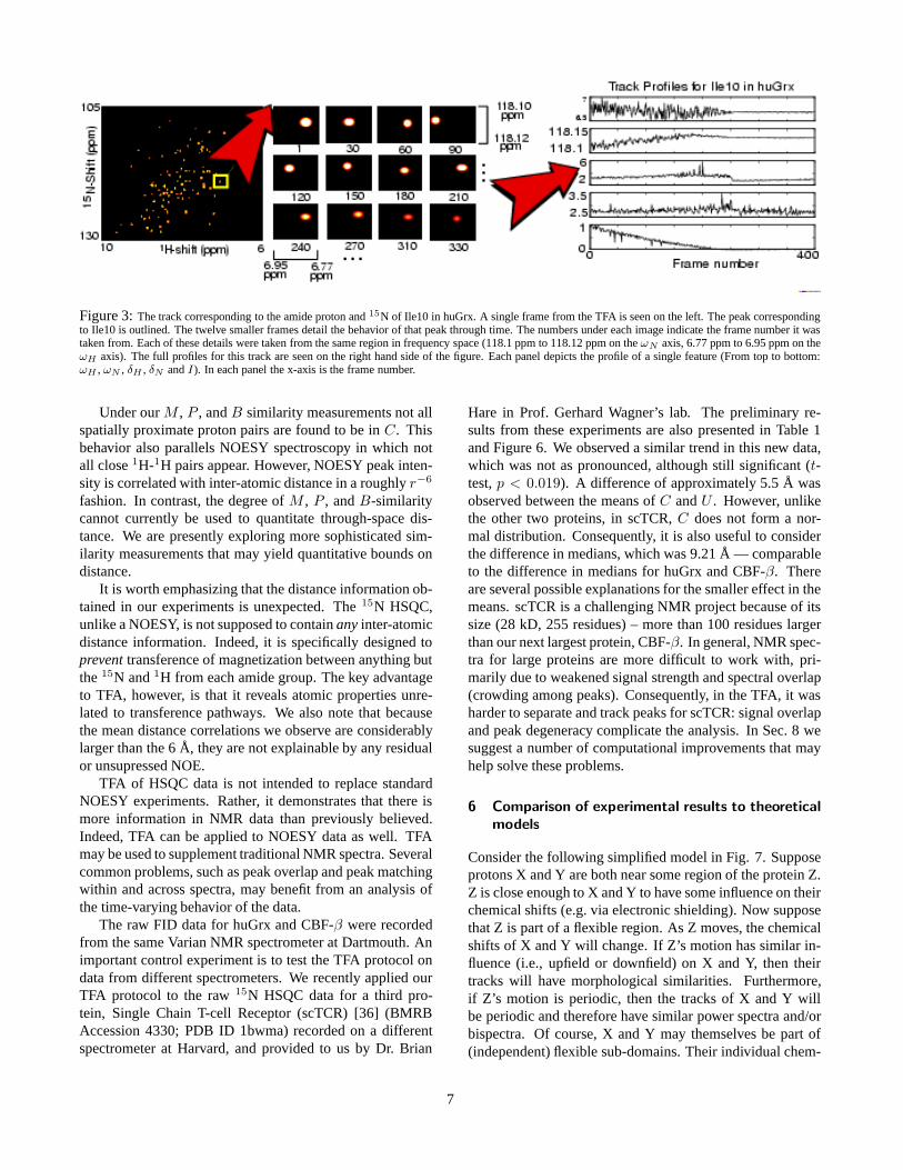
Figure 3: The track corresponding to the amide proton and 15N of Ile10 in huGrx. A single frame from the TFA is seen on the left. The peak correspondingto Ile10 is outlined. The twelve smaller frames detail the behavior of that peak through time. The numbers under each image indicate the frame number it wastaken from. Each of these details were taken from the same region in frequency space (118.1 ppm to 118.12 ppm on the ωN axis, 6.77 ppm to 6.95 ppm on theωH axis). The full profiles for this track are seen on the right hand side of the figure. Each panel depicts the profile of a single feature (From top to bottom:ωH , ωN , δH , δN and I). In each panel the x-axis is the frame number.

Under our M , P , and B similarity measurements not allspatially proximate proton pairs are found to be in C. Thisbehavior also parallels NOESY spectroscopy in which notall close 1H-1H pairs appear. However, NOESY peak inten-sity is correlated with inter-atomic distance in a roughly r−6

fashion. In contrast, the degree of M , P , and B-similaritycannot currently be used to quantitate through-space dis-tance. We are presently exploring more sophisticated sim-ilarity measurements that may yield quantitative bounds ondistance.

It is worth emphasizing that the distance information ob-tained in our experiments is unexpected. The 15N HSQC,unlike a NOESY, is not supposed to contain any inter-atomicdistance information. Indeed, it is specifically designed toprevent transference of magnetization between anything butthe 15N and 1H from each amide group. The key advantageto TFA, however, is that it reveals atomic properties unre-lated to transference pathways. We also note that becausethe mean distance correlations we observe are considerablylarger than the 6 Å, they are not explainable by any residualor unsupressed NOE.

TFA of HSQC data is not intended to replace standardNOESY experiments. Rather, it demonstrates that there ismore information in NMR data than previously believed.Indeed, TFA can be applied to NOESY data as well. TFAmay be used to supplement traditional NMR spectra. Severalcommon problems, such as peak overlap and peak matchingwithin and across spectra, may benefit from an analysis ofthe time-varying behavior of the data.

The raw FID data for huGrx and CBF-β were recordedfrom the same Varian NMR spectrometer at Dartmouth. Animportant control experiment is to test the TFA protocol ondata from different spectrometers. We recently applied ourTFA protocol to the raw 15N HSQC data for a third pro-tein, Single Chain T-cell Receptor (scTCR) [36] (BMRBAccession 4330; PDB ID 1bwma) recorded on a differentspectrometer at Harvard, and provided to us by Dr. Brian

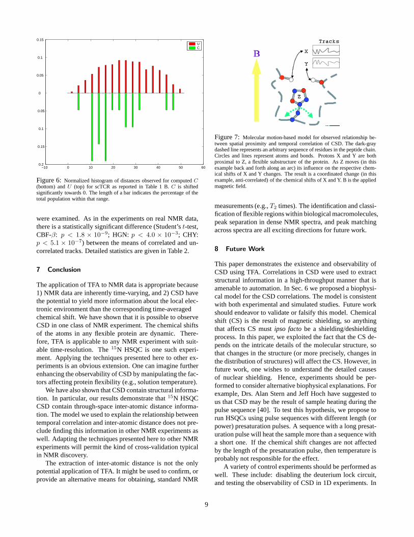
Hare in Prof. Gerhard Wagner’s lab. The preliminary re-sults from these experiments are also presented in Table 1and Figure 6. We observed a similar trend in this new data,which was not as pronounced, although still significant (t-test, p < 0.019). A difference of approximately 5.5 Å wasobserved between the means of C and U . However, unlikethe other two proteins, in scTCR, C does not form a nor-mal distribution. Consequently, it is also useful to considerthe difference in medians, which was 9.21 Å — comparableto the difference in medians for huGrx and CBF-β. Thereare several possible explanations for the smaller effect in themeans. scTCR is a challenging NMR project because of itssize (28 kD, 255 residues) – more than 100 residues largerthan our next largest protein, CBF-β. In general, NMR spec-tra for large proteins are more difficult to work with, pri-marily due to weakened signal strength and spectral overlap(crowding among peaks). Consequently, in the TFA, it washarder to separate and track peaks for scTCR: signal overlapand peak degeneracy complicate the analysis. In Sec. 8 wesuggest a number of computational improvements that mayhelp solve these problems.

6 Comparison of experimental results to theoretical

models

Consider the following simplified model in Fig. 7. Supposeprotons X and Y are both near some region of the protein Z.Z is close enough to X and Y to have some influence on theirchemical shifts (e.g. via electronic shielding). Now supposethat Z is part of a flexible region. As Z moves, the chemicalshifts of X and Y will change. If Z’s motion has similar in-fluence (i.e., upfield or downfield) on X and Y, then theirtracks will have morphological similarities. Furthermore,if Z’s motion is periodic, then the tracks of X and Y willbe periodic and therefore have similar power spectra and/orbispectra. Of course, X and Y may themselves be part of(independent) flexible sub-domains. Their individual chem-

7

0 0.8 18

10

12

14

16

18

Similarity

Dis

tan

ce

in

An

gstr

om

shuGRX Mean Distance vs Similarity

Mean Distance + Standard Error−Standard Error

0 0.8 15

10

15

20

25

Similarity

Dis

tan

ce

in

An

gstr

om

s

CBF−Beta Mean Distance vs Similarity

Mean Distance + Standard Error−Standard Error

Figure 4: Mean inter-atomic distance vs. similarity for huGrx (top panel)and CBF-β (bottom panel). The data-points were obtained by sweepingthe similarity threshold from 0 to 1 and computing the mean inter-atomicdistance for the set C corresponding to that threshold. The data-point at thefar left comprises all pairs of protons. The point at the far right comprisesonly those pairs of protons with highest similarity. To avoid an unfair skewin the mean, a proton and itself (i.e., similarity =1.0, distance = 0.0 Å)are not included in any computed C. The similarity scale is non-linearto highlight the drop in distance at high levels of similarity. Above 0.8we observe a steeper drop-off. The dashed lines are positive and negativestandard error measurements.

ical shifts may reflect the combined influence of multiple Z’splus tumbling and solvent interactions. However, insofar asour model is concerned, these additional factors will yieldmore complex CSD but the possibility of detecting correla-tions remains. In such cases, a multi-dimensional similaritymeasurement, such as the one presented here, will increasethe chances of finding correlations.

Z can only influence the chemical shifts of atoms withina fixed radius [37]. When this radius can be estimated, up-per bounds on the distance between temporally-correlatedtracks can be calculated and applied quantitatively in a man-ner analogous to NOE’s. Note that under this model, theconditions necessary to produce temporal correlations be-tween pairs of tracks are quite restrictive. In particular, itdoes not predict that all pairs of close atoms will be tempo-rally correlated.

0 5 10 15 20 25 30 35 40 450

0.05

0.1

0.15

0.2

0.25

0.3

0.35

% o

f D

istr

ibutio

n

Distance in Angstroms

huGrx

CU

0 10 20 30 40 50 600

0.1

0.2

0.3

0.4

0.5

% o

f D

istr

ibutio

n

Distance in Angstroms

CBFBeta

CU

Figure 5: Normalized histograms of distances observed for computedC’s and U ’s for huGrx (top panel) and CBF-β (bottom panel) as reportedin Table 1 B. In both panels, C is shifted significantly towards 0. The heightof a bar indicates the percentage of the total population within that range.

6.1 Comparison to Simulation of Chemical Shifts in

Mobile Protein Domains

We tested our model with simulated spectra of proteins inwhich we simulate the molecular dynamics over time. Inthe first simulation we created a time-series from twentyPDB files describing distinct, but similar, low-energy con-formations of CBF-β derived from traditional NMR struc-tural techniques. In the second simulation we used the time-series generated from the ten PDB files of hemoglobin (HGN)and Che-Y protein (CHY) as obtained from the database ofmolecular motions [15]. Using the program SHIFTS [38] wesimulated the chemical shifts for each proton in each of thePDB files describing the motion of the molecules. SHIFTStakes as input a PDB file and estimates proton chemical shiftsfrom empirical formulas. The result is analogous to TFAof real NMR data but not identical. A key distinction isthe length of the simulated tracks. Ten and twenty data-point tracks are too sparse to perform meaningful spectralanalysis so we only considered the morphological similar-ity (M ) of the tracks. The pairwise track similarities underthe M similarity measurement were calculated. Two filterswere applied to the similarity matrix. The first filter ignoresany single track whose chemical shift profile range is belowa minimum threshold. In other words, we ignored tracksthat were essentially flat. The second filter ignored pairsof tracks whose respective CSD ranges were wildly differ-ent. That is, we did not compare a track with high activitywith one with low activity. The reason is that atoms ex-periencing wildly different ranges of CSD are unlikely tobe nearby. A threshold was applied to the filtered matrix.The inter-atomic distances of the tracks above the threshold

8

−10 0 10 20 30 40 50 60 0.2

0.15

0.1

0.05

0

0.05

0.1

0.15 UC

Figure 6: Normalized histogram of distances observed for computed C(bottom) and U (top) for scTCR as reported in Table 1 B. C is shiftedsignificantly towards 0. The length of a bar indicates the percentage of thetotal population within that range.

were examined. As in the experiments on real NMR data,there is a statistically significant difference (Student’s t-test,CBF-β: p < 1.8 × 10−9; HGN: p < 4.0 × 10−3; CHY:p < 5.1 × 10−7) between the means of correlated and un-correlated tracks. Detailed statistics are given in Table 2.

7 Conclusion

The application of TFA to NMR data is appropriate because1) NMR data are inherently time-varying, and 2) CSD havethe potential to yield more information about the local elec-tronic environment than the corresponding time-averagedchemical shift. We have shown that it is possible to observeCSD in one class of NMR experiment. The chemical shiftsof the atoms in any flexible protein are dynamic. There-fore, TFA is applicable to any NMR experiment with suit-able time-resolution. The 15N HSQC is one such experi-ment. Applying the techniques presented here to other ex-periments is an obvious extension. One can imagine furtherenhancing the observability of CSD by manipulating the fac-tors affecting protein flexibility (e.g., solution temperature).

We have also shown that CSD contain structural informa-tion. In particular, our results demonstrate that 15N HSQCCSD contain through-space inter-atomic distance informa-tion. The model we used to explain the relationship betweentemporal correlation and inter-atomic distance does not pre-clude finding this information in other NMR experiments aswell. Adapting the techniques presented here to other NMRexperiments will permit the kind of cross-validation typicalin NMR discovery.

The extraction of inter-atomic distance is not the onlypotential application of TFA. It might be used to confirm, orprovide an alternative means for obtaining, standard NMR

Figure 7: Molecular motion-based model for observed relationship be-tween spatial proximity and temporal correlation of CSD. The dark-graydashed line represents an arbitrary sequence of residues in the peptide chain.Circles and lines represent atoms and bonds. Protons X and Y are bothproximal to Z, a flexible substructure of the protein. As Z moves (in thisexample back and forth along an arc) its influence on the respective chem-ical shifts of X and Y changes. The result is a coordinated change (in thisexample, anti-correlated) of the chemical shifts of X and Y. B is the appliedmagnetic field.

measurements (e.g., T2 times). The identification and classi-fication of flexible regions within biological macromolecules,peak separation in dense NMR spectra, and peak matchingacross spectra are all exciting directions for future work.

8 Future Work

This paper demonstrates the existence and observability ofCSD using TFA. Correlations in CSD were used to extractstructural information in a high-throughput manner that isamenable to automation. In Sec. 6 we proposed a biophysi-cal model for the CSD correlations. The model is consistentwith both experimental and simulated studies. Future workshould endeavor to validate or falsify this model. Chemicalshift (CS) is the result of magnetic shielding, so anythingthat affects CS must ipso facto be a shielding/deshieldingprocess. In this paper, we exploited the fact that the CS de-pends on the intricate details of the molecular structure, sothat changes in the structure (or more precisely, changes inthe distribution of structures) will affect the CS. However, infuture work, one wishes to understand the detailed causesof nuclear shielding. Hence, experiments should be per-formed to consider alternative biophysical explanations. Forexample, Drs. Alan Stern and Jeff Hoch have suggested tous that CSD may be the result of sample heating during thepulse sequence [40]. To test this hypothesis, we propose torun HSQCs using pulse sequences with different length (orpower) presaturation pulses. A sequence with a long presat-uration pulse will heat the sample more than a sequence witha short one. If the chemical shift changes are not affectedby the length of the presaturation pulse, then temperature isprobably not responsible for the effect.

A variety of control experiments should be performed aswell. These include: disabling the deuterium lock circuit,and testing the observability of CSD in 1D experiments. In

9

addition, we would like to test our protocol on a number ofother proteins under different conditions. Therefore we in-vite NMR structural biologists interested in a rapid structuralassay to contact us.

Finally, a number of computational improvements arepossible. The short-time FT has some disadvantages, suchas the limit in its time-frequency resolution capability. Onemight overcome these limitations by the use of wavelet the-ory [16]. This should help in applying TFA to larger pro-teins, as should improved peak-tracking and better track mod-eling.

References

1. C. Bailey-Kellogg, A. Widge, J. J. Kelley III, M. Berardi, J. Bushweller,B. R. Donald, "The NOESY Jigsaw: Automated Protein Secondary Struc-ture and Main-Chain Assignment from Sparse, Unassigned NMR Data, 4thAnnual Intl. Conf. on Comp. Mol. Biol., Tokyo, Japan, pp. 33-44, (2000)

2. C. Bailey-Kellogg, A. Widge, J. J. Kelley III, M. Berardi, J. Bushweller,B. R. Donald, "The NOESY Jigsaw: Automated Protein Secondary Struc-ture and Main-Chain Assignment from Sparse, Unassigned NMR Data,J. Computational Biology, 7(3-4) (2000) pp. 537-558.

3. D.E. Zimmerman, C.A. Kulikowski, Y. Huang, W. Feng, M. Tashiro, S.Shimotakahara, C. Chien, R. Powers, and G. Montelione. Automated anal-ysis of protein NMR assignments using methods from artificial intelligence.J. Mol. Bio, 269:592-610, 1997.

4. C. Bartels, P. Guntert, M. Bileter, and K. Wuthrich. GARANT— a gen-eral algorithm for resonance assignment of multidimensional nuclear mag-netic resonance spectra. J. Comp. Chem., 18:139-149, 1997

5. D. Croft, J. Kemmink, K.-P. Neidig, and H. Oschkinat. Tools for theautomated assignment of high-resolution three-dimensional protein NMRspectra based on pattern recognition techniques. J. Biomol. NMR, 10:207-219, 1997

6. Y. X. Lin and G. Wagner, Efficient side-chain and backbone assignmentin large proteins: Application to tGCN5, J. Biomol. NMR, 15 227-239,1999.

7. J.A. Cuff, M.E. Clamp, A.S. Siddiqui, M. Finlay, and G.J. Barton.JPRED: A consensus secondary structure prediction server. Bioinformat-ics, 14:892-893. 1998.

8. G. Dealeage, B. Tinland, and B. Roux. A computerized version of theChou and Fasman method for predicting the secondary structure of proteins.Analytical Biochemistry, 163(2):292-297, June 1987

9. D.S. Wishart, B.D. Sykes, and F.M. Richards. The chemical shift index:a fast and simple method for the assignment of protein secondary struc-ture through NMR spectroscopy. Biochemistry, 31(6):1647-1651, February1992

10. K. Wüthrich, NMR of Proteins and Nucleic Acids. (John Wiley & Sons,1986).

11. J. Cavanagh, W.J. Fairbrother, A.G. Palmer, N.J. Skelton, Protein NMRSpectroscopy: Principles and Practice. 416-418 (Academic Press Inc.,1996).

12. Sitkoff, D., & Case, D. Density Functional Calculations of ProtonChemical Shifts in Model Peptides. J. Am. Chem Soc. 119, 12262-12273(1997)

13. Dejaegere, A. P., Case, D. Density Functional Study of Ribose andDeoxyribose Chemical Shifts, J. Phys. Chem. A 102, 5280-5289 (1998)

14. Moravetski, V., Hill, J. R., Eichler, U., Sauer, J. 29Si NMR ChemicalShifts of Silicate Species: Ab Initio Study of Environment and StructureEffects, J. Am. Chem. Soc. 118, 13015-13020 (1996)

15. M. Gerstein and W. Krebs, Nucleic Acids Research 26 (1998).

16. Serrai, H., L. Senhadji, J. D. de Certaines, and J. L. Coatrieux, Time-domain quantification of amplitude, chemical shift, apparent relaxation timeT ∗

2, and phase by wavelet-transform analysis. Application to biomedical

magnetic resonance spectroscopy J. Magn. Res. 124, 20-34 (1997).

17. Wagner, G., NMR relaxation and protein mobility, Current Opinion inStruct. Biol., 3, 748-754 (1993)

18. Palmer, A. G., Williams, J., & McDermott, A. Nuclear Magnetic Reso-nance Studies of Biopolymer Dynamics, J. Phys. Chem., 100, 13293-13310(1996)

19. Lipari, G. & Szabo, A., Model-Free approach to the Interpretation ofNuclear Magnetic Resonance Relaxation in Macromolecules. 1. Theoryand Range of Validity, J. Am. Chem. Soc., 104, 4546-4559 (1982)

20. Palmer, A. G., Dynamic properties of proteins from NMR spectroscopy,Current Opinion in Biotechnology., 4, 385-391 (1993)

21. Palmer, A. G., Probing molecular motion by NMR, Current Opinion inStruct. Biol., 7, 732-737 (1997)

22. Lipari, G. & Szabo, A., Model-Free approach to the Interpretation ofNuclear Magnetic Resonance Relaxation in Macromolecules. 2. Analysisof Experimental Results, J. Am. Chem. Soc., 104, 4560-4570 (1982)

23. Kay, L., Protein Dynamics from NMR, Nature Struct. Biol. NMRSupplement, July (1998)

24. Palmer, A. G. and Bracken, C. Spin Relaxation Methods for Charac-terizing Picosecond-nanosecond and microsecond-millisecond motions inProteins, in NMR in Supramolecular Chemistry, Pons, M. ed. 171-190,(1999 Kluwer Academic Publishers, Netherlands)

25. A.V. Oppenheim and R.W. Schafer, Discrete-Time Signal Processing(Prentice Hall, 1989)

26. Delaglio, F. et al, NMRPipe: a multidimensional spectral processingsystem based on UNIX Pipes. J. Biomol. NMR. 6 (1995).

27. Mendel, J. M., Tutorial on Higher-Order Statistics (Spectra) in SignalProcessing and System Theory: Theoretical Results and Some Applica-tions, Proc. IEEE, 79 278-305 (1996).

28. H. Farid, Blind Inverse Gamma Correction, IEEE Trans. on ImageProcessing

29. Sun, C., Holmgren, A. & Bushweller, J., Complete 1H, 13C, and 15NNMR resonance assignments and secondary structure of human glutare-doxin in the fully reduced form, Protein Science, 6, 383-390 (1997)

30. Sun, C., Berardi, M. J., & Bushweller, J., The NMR solution structureof human glutaredoxin in the fully reduced form. J. Mol. Bio 280, p 687(1998).

31. Huang, X., Speck, N. A. & Bushweller, J., Complete Resonance As-signments and secondary structure of core binding factor β, J. Biom. NMR12, 459-460 (1997).

32. Huang, X. Peng, J., Speck, N. A. & Bushweller, J., Solution Structure ofCore Binding Factor Beta and Map of the CBF-α Binding Site, Nat StructBiol. 6 pp. 624 (1999)

33. Bloch, F., Hansen, W.W. & Packard, M., Nuclear Induction, Phys. Rev.69,127 (1946).

34. Wijmenga, S. S., Kruithof, M. & Hilbers, C. W., Analysis of 1H chem-ical shifts in DNA: Assessment of the reliability of 1H chemical shifts foruse in structure refinement. J. Bio NMR 10, 337-350 (1997)

35. J. Cavanagh, W.J. Fairbrother, A.G. Palmer, N.J. Skelton, Protein NMRSpectroscopy: Principles and Practice. 384-394 (Academic Press Inc.,1996).

36. Hare B.J., Wyss D.F., Osburne M.S., Kern P.S., Reinherz E.L., WagnerG. Structure, specificity and CDR mobility of a class II restricted single-chain T-cell receptor, Nat Struct Biol 1999 Jun;6(6):574-81

37. Pearson, J. G., et al Predicting Chemical Shifts in Proteins: StructureRefinement of Valine Residues by Using ab Initio and Empirical GeometryOptimizations, J. Am. Chem. Soc. 119, 11941-11950 (1997)

38. Osapay, K. & Case, D.A., Peptides, Chemistry, Structure and Biology,R.S. Hodges and J.A. Smith, eds. (Leiden: ESCOM, 1994), pp. 911-913.

10

39. Xu, Y. et al, Protein Structure Determination using Protein Threadingand Sparse NMR Data, 4th Annual Intl. Conf. on Comp. Mol. Biol., Tokyo,Japan, pp. 299-307, (2000)

40. Stern, A., and J. C. Hoch, Personal communication (2000).

Acknowledgments

We thank Hany Farid and Chris Bailey-Kellogg for their as-sistance on the algorithmic and signal processing aspects ofthis work, Brian Hare, Gerhard Wagner, John Bushweller,Chaohong Sun, and Xuemei Huang for generously provid-ing us their NMR data, Marcelo Berardi, Jack Kelley, BrianHare, Alan Stern, Jeff Hoch, Sven Hyberts, Dave Rovnyak,Hiroshi Matsuo, Gerhard Wagner, Souheil Inati, and JohnBushweller for their insights into NMR, Deborah Chiavelliand Jennifer Groh for feedback on the statistical aspects ofthis work and Fred Henle for his assistance in preparing thispaper. We thank the RECOMB referees, Tomás Lozano-Pérez, Amy Anderson, and all members of Donald Lab fortheir insightful suggestions and comments. This work issupported by the following grants to B.R.D.: National Sci-ence Foundation grants IIS-9906790, EIA-9901407, EIA-9802068, CDA-9726389, EIA-9818299, CISE/CDA-9805-548, IRI-9896020, and IRI-9530785, U. S. Department ofJustice contract 2000-DT-CX-K001, and an equipment grantfrom Microsoft Research.

Appendix

Table 2 shows the detailed results of temporal similarity mea-surements on simulated NMR data. Figure 8 shows the re-lationship between the differences in inter-atomic mean dis-tances between the sets C and U and the size of the corre-lated set C. Figure 9 shows ribbon diagrams of both test pro-teins and the distance restraints derived via TFA projectedonto cartoons of those proteins.

CBF-β CHY HGN

C (Å) U (Å) C (Å) U (Å) C (Å) U (Å)

Mean 9.78 21.70 13.78 17.35 13.30 18.67

Median 4.84 20.46 13.58 17.40 13.21 18.65

Max 26.26 55.96 23.10 34.02 22.66 40.34

Min 2.96 2.58 2.87 2.63 2.83 2.60

Pairs 24 18608 22 7728 44 8867

t-test p < 1.8 × 10−9 p < 4.0 × 10−3 p < 5.1 × 10−7

Table 2: Inter-atomic distance statistics for the distributionof temporally correlated protons (C) vs. uncorrelated pro-tons (U ) in simulated CBF-β, CHY and HGN spectra. Thesimulation of CBF-β spectrum is based on twenty PDB filesencoding NMR-derived low-energy conformations. Thesetwenty low-energy conformations are derived from NMRdata and were averaged to obtain the final, published struc-ture of CBF-β [32]. We consider these conformations toform an ergodic ensemble. That is, each conformation isdrawn from some low-energy well in conformation spaceand any path through these conformations is equally likely.Consequently, we generated a time series by using each con-formation once, in random order. We report the results ofone random permutation of the conformations but tests with100 other random permutations yield similar results. Thesimulation of the CHY and HGN spectra is based on tenPDB files (for each protein) depicting conformations gen-erated by molecular dynamics simulation. Student’s t-testconfidence scores (p-values) reflect the probability the dif-ferences in means are due to chance. The effects of thesmaller sample size for CHY and HGN relative to CBF-βare seen in the difference in means between C and U . Theshorter series have less power for discrimination, but the sta-tistical significance remains.

0

20

1 02

6

0

8

1 02

9

Threshold Threshold

CBF-β huGrx

log

(# p

airs

)

log

(# p

airs

)

∆-M

ea

ns (

A)

˚

∆-M

ea

ns (

A)

˚

Figure 8: Normalized Similarity Threshold vs. difference inmeans of C and U (solid line) and cardinality of C (dashedline) for CBF-β and huGrx. The x-axis is a normalizedthreshold over the multidimensional M , P , and B-similaritymeasurements. Within the range of thresholds presentedhere, the distributions C and U are statistically different (i.e.,they pass a t-test). As the similarity threshold increases, thecardinality of C decreases and the difference in means in-creases.

11

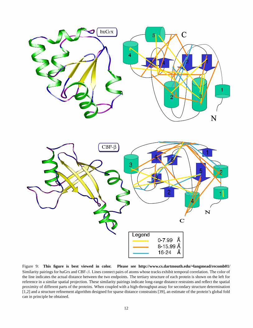
Figure 9: This figure is best viewed in color. Please see http://www.cs.dartmouth.edu/˜langmead/recomb01/Similarity pairings for huGrx and CBF-β. Lines connect pairs of atoms whose tracks exhibit temporal correlation. The color ofthe line indicates the actual distance between the two endpoints. The tertiary structure of each protein is shown on the left forreference in a similar spatial projection. These similarity pairings indicate long-range distance restraints and reflect the spatialproximity of different parts of the proteins. When coupled with a high-throughput assay for secondary structure determination[1,2] and a structure refinement algorithm designed for sparse distance constraints [39], an estimate of the protein’s global foldcan in principle be obtained.

12