Extracting stay regions with uncertain boundaries fromGPS trajectories: a case study in animal ecology

Maria Luisa Damiani & Hamza IssaDept. Computer Science

University of Milan, Milan, Italy{damiani,issa}@di.unimi.it

Francesca CagnacciDept. Biodiversity and Molecular Ecology

Fondazione Edmund MachS. Michele all’Adige, Italy

francesca.cagnacci@fmach.it

ABSTRACTIn this paper we present a time-aware, density-based cluster-ing technique for the identification of stay regions in trajec-tories of low-sampling-rate GPS points, and its applicationto the study of animal migrations. A stay region is defined asa portion of space which generally does not designate a pre-cise geographical entity and where an object is significantlypresent for a period of time, in spite of relatively short pe-riods of absence. Stay regions can delimit for example theresidence of animals, i.e. the home-range. The proposedtechnique enables the extraction of stay regions representedby dense and temporally disjoint sub-trajectories, throughthe specification of a small set of parameters related to den-sity and presence. While this work takes inspiration fromthe field of animal ecology, we argue that the approach canbe of more general concern and used in perspective in dif-ferent domains, e.g. the study of human mobility over largetemporal scales. We experiment with the approach on acase study, regarding the seasonal migration of a group ofroe deer.

Categories and Subject DescriptorsH.2.8 [Database management]: Database applications—Spatial databases and GIS

General TermsAlgorithms, experimentation

KeywordsMobility patterns, clustering, animal ecology

1. INTRODUCTIONWith the advances in mobile technologies, the extraction

of behavioral patterns from collections of geometric trajec-tories regarding e.g. people, animals and goods, has becomea prominent research issue in a variety of disciplines such

Permission to make digital or hard copies of all or part of this work forpersonal or classroom use is granted without fee provided that copies are notmade or distributed for profit or commercial advantage and that copies bearthis notice and the full citation on the first page. Copyrights for componentsof this work owned by others than ACM must be honored. Abstracting withcredit is permitted. To copy otherwise, or republish, to post on servers or toredistribute to lists, requires prior specific permission and/or a fee. Requestpermissions from Permissions@acm.org.SIGSPATIAL’14, November 04 - 07 2014, Dallas/Fort Worth, TX, USACopyright 2014 ACM 978-1-4503-3131-9/14/11$15.00http://dx.doi.org/10.1145/2666310.2666417.

as geography, transportation science, biology, computer sci-ence [1, 2, 3, 4]. For example, in the field of animal ecology,modern animal telemetry and sensor networks (e.g. GPSreceivers and other sensors mounted on devices deployed onanimals, such as collars) enable the collection of content-rich, fine-grained trajectories, opening up new opportunitiesfor the study of the animal behavior [5]. In particular thispaper takes inspiration from the migration patterns of wildanimals. Analyzing animal mobility offers a number of ad-vantages over e.g. human mobility. For example privacy isnot an issue, thus mobility data can be freely shared withinthe research community, moreover the solutions can be vali-dated using field work knowledge and experience. This pavesthe way to the development of effective techniques and totheir deployment in different domains. In this spirit, wepresent a generic problem, and develop a solution which isdeployed and evaluated on a case study in animal ecology.

1.1 Case studyThe case study regards the extraction of the seasonal mi-

grations of a number of roe deer (small ungulate species thatcan live in a variety of environments), equipped with a low-sampling-rate GPS collar and tracked for a period coveringa few seasons. The animals of this species can either migrateor be stationary, a behavior known as partial migration [6].Moreover, whenever an animal migrates, the migration takesplace with modalities and times that - although respectingcertain general patterns, e.g. seasonality - can vary fromanimal to animal. This means that every animal has itsown migration behavior (i.e. the movement pattern is indi-vidual [1]). At very coarse level, the behavior can be seenas a stop-and-move pattern [7], i.e. the animal stays in aregion for some time and then moves to some other region.In reality the behavior is more complex. The animals spendmost of their time inside a home-range. The concept ofhome-range is key in animal ecology. A popular definitionof home-range is that of ”area traversed by the individualin its normal activities of food gathering, mating and car-ing for young” [8]. In reality, the concept does not have aunivocal interpretation (the interested reader can refer to[9] for details). Occasionally the animals can make excur-sions outside the home-range and possibly stay for shortperiods in a different area before returning to the home-range. A migration is a transition from one home-range toanother home-range. During the migration the animal canstop in small areas for a short time (stopover). An exampleof migration pattern, which combines all these concepts, isreported in Figure 1(a). Note that the migration behavior

Figure 1: Example of animal migration pattern.

does not necessarily have a periodicity (e.g. animals maynot migrate every year). Moreover the temporal and spatialextent of the regions in which the animals stay, as well asthe duration of the moves can significantly vary [10]. As amatter of fact, there is no consensus in the scientific commu-nity on the fact that the distances covered by the animalsof this species or their speed are good indicators of a migra-tion in progress, while the collection of GPS traces, as formost middle to large vertebrate species, is a relatively recentpractice, that needs to be still fully exploited in its poten-tialities. A remarkable initiative in this field is Eurodeer, acollaborative project started in 2009 and involving 29 Euro-pean research institutes for the collection, organization andsharing of movement data, i.e. GPS, VHF and activity data,regarding over 900 roe deer in 25 areas in Europe1. The Eu-rodeer project [10] provides the application context for theresearch presented in this paper.

1.2 RequirementsWe take inspiration from the case study to define a generic

problem framework where: (i) we propose the concept ofstay region to abstract away from the notion of animal’shome-range, stopover and so on; (ii) the problem to addressis to extract stay regions from low-sampling-rate GPS tra-jectories. In particular, we define stay region as a sequenceof points spatially confined to a portion of space (not desig-nating a geographical entity, e.g. forest), frequently visitedby the object and in which the object spends sufficient timealthough experiencing periods of absence. No assumption ismade on speed and other movement characteristics, as wellon the distribution of points in stay regions.

A stay region is naturally an area that is dense of points.Density however is not sufficient to characterize a stay re-gion, as an object is also requested to stay for sufficienttime in the region. A straightforward interpretation of thenotion of ”time elapsed in a region” is that of stay duration,the time difference between the last point and first pointin the region. In reality, since the object can occasionallyleave the stay region, the time effectively spent in the regionis very likely shorter than the duration. Ideally, an objectrepeatedly moving back and forth between two areas, sayA and B does not stay in any of the two regions, becausethere is no evidence that the individual remains for sufficienttime in any of them. To capture this intuition we introducethe notion of presence. The presence in a stay region is thetime plausibly elapsed in such a region. Plausibly meanswith reasonable evidence, given the uncertainty of the ob-ject location. Accordingly a stay region is a sub-trajectorydefining a region which is dense and in which the object’s

1http://www.eurodeer.org

presence is significant.The problem to address can be finally formulated as fol-

lows. The goal is to extract the sequence of stay regionsfrom a trajectory, considering that: (i) the stay regions areto be temporally disjoint, i.e. the temporal extent of a stayregion does not overlap the temporal extent of another stayregion. (ii) The number of stay regions in a trajectory isnot known. (iii) Stay regions can have an arbitrary spa-tial shape while the temporal extent can be only coarselypredicted. (iv) Periods of presence and absence in a regioninterleave. (v) Mobility parameters, e.g. speed, direction,are not relevant to discriminate whether the object is insideor outside a stay region.

1.3 Approach and contributionOne could argue that the problem is not very different

from detecting e.g. the points of interest visited by touristssuch as in [3, 11]. For example Zheng et al. [3], definesa stay point as a set of consecutive GPS points of the tra-jectory, close to each other (based on distance threshold)and in which the user stays for a minimum time (durationthreshold). The temporal scale at which the movement is ob-served is however a small scale (e.g. hours, days), moreoverthe semantics of the stay points is given by the geographicalcontext. Conversely, in the case study the animals can stayin a region for months or years, and exhibit a complex be-havior, such as moving back and forth from a region whosespatial and temporal boundaries are uncertain.

A different paradigm is trajectory segmentation [12, 13,14, 15, 16]. Trajectory segmentation is extensively applied toextract stop-and-move patterns such as in [14, 13]. The ideaof segmentation is to partition the trajectory in segments ofmaximal length where movement characteristics inside eachsegment are monotone i.e. the same characteristics hold inevery subsegment of the segment [12]. Monotone character-istics include speed, heading, curviness. One could define,for example, a stay region as a segment is which the object’sspeed is below a threshold value. Unfortunately, there is noscientific or empirical evidence that these movement char-acteristics are really informative for the migration patternwe are considering (while it can be for specific migrationpatterns as in [17]). On a different front, density-based clus-tering is a popular and robust paradigm that has shown tobe effective in various contexts including stream data analy-sis and data warehousing [18, 19, 20, 21]. It is worth notingthat density-based clustering is also employed for the discov-ery of stops (i.e. low speed segments) in fine-grained humantrajectories as in [22, 13]. The key idea behind those solu-tions is to extend the notion of distance to account of thetemporal dimension (i.e. a cluster consists of points that areclose both in space and time). We claim that such distancemodel is conceptually inadequate in our scenario. In fact,animals can experience periods of absence from the homerange, thus subsequent points in the cluster are not neces-sarily close in time. In essence, constraining the temporaldistance is not a solution, while we need to ensure that stayregions do not overlap in time while satisfying the presencerequirements.

In this paper, we present a novel approach which combinesthe effectiveness of density-based clustering with the parti-tioning capability of trajectory segmentation without intro-ducing any supplementary assumption on movement char-acteristics. The key idea is to only use density and presence

as non-monotone criteria for the partitioning of a trajectoryin a set of sub-trajectories of maximal length and tempo-rally non-overlapping. A trajectory is subdivided in piecesalternating stay regions and non-stay regions. The key con-tributions of this paper can be summarized as follows:

• We introduce and define in a rigorous way the stayregions discovery problem.

• We develop a novel algorithm to extract the stay re-gions. The algorithm is grounded on the formal frame-work of DBSCAN [18]. The algorithm requires thespecification of only three parameters. This facilitatesthe practical deployment of the technique. The algo-rithm is called SeqScan.

• We validate the algorithm on the case study, specifi-cally regarding the behavior of a few tens of roe deerliving in the same area, showing that the algorithmeffectively detects migratory behavior previously de-scribed by means of statistics-based methods [10], andhelps explaining uncertain cases. Moreover we illus-trate a possible methodology of use.

The remainder of the paper is organized as follows: the re-search problem is formally defined in Section 2. Section 3describes the algorithm. Section 4 presents the experimentalpart, mostly focused on the application of the technique onthe case study. Section 6 overviews related research. Theconclusive section discusses the plans for future work.

2. PROBLEM DEFINITIONBefore defining the stay region discovery problem, we re-

view the fundamental concepts of DBSCAN and provide afew basic definitions.

2.1 Background: the DBSCAN cluster modelConsider a database P of points and the input parameters

ε ∈ R (i.e. the distance threshold), and K ∈ N (i.e. theminimum number of points that a cluster contains). Let d()be the distance function.

The fundamental concepts of the DBSCAN cluster modelare as follows [18]: (i) The ε-neighborhood of p ∈ P , de-noted Nε(p), is the subset of points that are ”close” to p,i.e. Nε(p) = {pi ∈ P, d(p, pi) ≤ ε}. (ii) Point p is a corepoint if its ε-neighborhood contains at least K points, i.e.|Nε(p)| ≥ K. A point that is not a core point but belongs tothe neighborhood of a core point is a border point. (iii) Pointp is directly density-reachable from q if q is a core point andp ∈ Nε(q). (iv) Two points p and q are density reachableif there is a chain of points p1, .., pn, p1 = p, pn = q suchthat pi+1 is directly reachable from pi. (v) Points p and qare density connected if there exists a core point o such thatboth p and q are density-reachable by o. A cluster is finallydefined as a maximal set of density-connected points, wheremaximal means that every point p that is reachable from acore point q belongs to the cluster containing q.

2.2 PreliminariesTrajectory. A trajectory T is a sequence of spatio-tempo-

ral points T = [p1, .., pn] with pi = (li, ti) where li, ti isthe sampled location in space and time respectively withti < ti+1 and n the length of the trajectory. The trajectoryhas a begin point pstart, an end point pend, a temporal ex-tent [tstart, tend], and a duration |tstart−tend|. The duration

is measured in e.g. days or in some other unit. No assump-tion is made on the sampling rate. However the distance inspace covered by the object in the time interval [ti, ti+1] isnormally limited (in relation to the mobility pattern underconsideration).

Sub-trajectory. A sub-trajectory S = [p1i , .., pmj ] ⊆ T

of length m is a sequence of temporally ordered points ofT with index 1, ..,m. A sub-trajectory may contain gaps.A gap is the open interval (ti, tj) signing a ”hole” in thesequence, i.e. two points that are consecutive in S are notconsecutive in T , i.e. pxi , p

x+1j ∈ S → j 6= i+1. For example,

given T = [p1, .., p9] the sub-trajectory [p3, p5, p8] containstwo gaps, (t3, t5) and (t5, t8), respectively. The temporalextent of the sub-trajectory is [t3, t8].

(a)

(b)

Figure 2: (a) Space-time cube of the example trajectory. (b)The points are projected on space. A subset of points formsa dense region with respect to ε,K = 3

2.3 The stay region discovery problemThe notion of stay region is defined in terms of density

and presence.

2.3.1 Dense regionA dense region in T is a sub-trajectory consisting of points

that, projected on the plane, forms a DBSCAN cluster. Letd(.) be the Euclidean distance. Formally:

Definition 2.1 (Dense region). A dense region S ⊆T is a sub-trajectory S = [q1, .., qm] such that the set oflocations [l1, .., lm] is a maximal density connected set withrespect to ε and K. The points that do not belong to anydense region in T are qualified as noise. �

Example 2.1. Consider the trajectory T = [p1, .., p9] il-lustrated in the space-time cube of Figure 2.1(a). The pointsprojected on the plane are shown in Figure 2.1(b) and num-bered following the temporal order. For the sake of readabil-ity, the pairs of points that are at distance less than or equal εare connected by a line. The value of K is set to 3. It can benoticed that the sequence S = [p1, p4, p6, p7, p8, p9] is a denseregion.The points p4, p6, p7, p8 are core points while p1, p9 areborder points. The region S contains two gaps,representedby the open intervals (t1, t4) and (t4, t6).

2.3.2 PresenceA dense region S may contain gaps, where a gap indicates

a period of absence from the region. We call Time Segmentof a dense region the set of periods in which the object ispresent in such a region. A graphical representation of theTime Segment associated with the dense region in Example2.1 is shown in Figure 3. This Time Segment consists of twoinstants and one period (the instant is a degenerated periodwhere the two extremes coincide), i.e. [t1, t1]∪[t4, t4]∪[t6, t9].

Figure 3: The Time Segment of the dense region in Example2.1. The dotted lines indicate gaps. The circles correspondto instants.

Next, we introduce the notion of presence in incrementalfashion. Let us start considering the case in which pi, pi+1 ∈T are two consecutive points both included in the denseregion S. A sensible question is whether the intermediatepoints falling in the interval [ti, ti+1] belong to S or not. Weknow that the position is uncertain. Yet, we have assumedthat the object’s move between two subsequent samples isrelatively limited in space. This legitimates the assumptionthat if pi, pi+1 ∈ S also the points in the interval I = [ti, ti+1]are contained in S. Therefore the presence in I is computedas duration of I. Consider now the case in which only oneof the points is in S, namely the object moves somewhereoutside the area. In this case, it is plausible that the objectis outside the dense region for most of the time. In thiscase, the presence in I is set to 0. By extension, we definethe presence in S as the sum of the presence in each segmentof S. A formal definition is given below:

Definition 2.2 (Presence). Let S = [q1., .., qm] be adense region in T = {p1, .., pn}. Denote with S[i, i+ 1] twoconsecutive points in S. We define:

• The presence in S[i, i+ 1]:

P (S[i, i+1], T ) =

{|th − th+1|, if ∃h, qi = ph, q

i+1 = ph+1

0, otherwise

• The presence in the dense region S:

P (S, T ) =∑

i∈[1,n−1]

P (S[i, i+ 1], T )

• We say that the presence in S is persistent with respectto δ > 0 ( presence threshold) if it holds: P (S, T ) > δ�

The presence can be easily computed from the Time Seg-ment. For example, given the Time Segment in Figure 3 thepresence in the dense region is |t9 − t6|.

2.3.3 Problem formulation

Definition 2.3 (Stay region). A stay region S in thetrajectory T is a sub-trajectory of T such that: (i) S is adense region w.r.t. ε and K. (ii)The object’s presence in Sis persistent w.r.t δ

Following the previous definition, the problem to addressis to find the set of stay regions based on the values of thethree parameters: ε,K, δ. Fundamental requirements are:(i)the stay regions are to be temporally disjoint. This meansthat a point in a stay region falling in the temporal extent ofanother stay region cannot exist. (ii) The stay regions oughtto be of maximal length, that is if a point can be added toregion S, then it belongs to S. The problem is summarizedas follows:

Definition 2.4 (Stay regions discovery problem).The problem is to extract from a trajectory T the sequence[S1, .., Sn] of temporally disjoint stay regions of maximal length.The points that do not fall in any stay region are noise. Thesubset of noise points temporally falling between the end ofone stay region Si and the beginning of the next one Si+1

form a transition (denoted Si → Si+1).

The set of stay regions and transitions determines a parti-tion, i.e. segmentation, of the temporal extent of T .

3. THE ALGORITHMA naive approach to the above problem is to apply the DB-

SCAN algorithm [18] over the set of points (projected overspace) to find the set of dense regions and then determinethose in which the presence is persistent. The drawbackis that the resulting sub-trajectories are not temporally dis-joint. Thus the solution does not work. A different approachis to scan sequentially the trajectory and progressively ag-gregate the points creating one stay region at a time. Inthis case, the question is how to recognize the end of a stayregion. We recall, in fact, that no supplementary movementcharacteristic can indicate whether the object is inside oroutside a stay region. To deal with this problem, we pro-pose the following approach: (i) a stay region is seen as anattraction area, i.e. an area when the object returns afterperiods of absence. (ii) A stay region remains attractive forthe object until a new stay region is found. This means thatthe boundaries of a stay region are only known when thenext stay region is detected (or the trajectory terminates).

In the next, we refer to a stay region ”in progress” withthe term of cluster (not to be confused with the DBSCANcluster). Clusters are dynamic entities with a life cycle. Asillustrated in the state diagram in Figure 4 a cluster origi-nates from a dense region when the object’s presence getspersistent, then the cluster is expanded with new points, andfinally it is closed. The event that indicates the terminationof the cluster expansion is the starting of a new and morerecent cluster. At any instant, there is thus at most oneactive cluster and possibly one or more closed clusters. Thealgorithm is described in the next.

Figure 4: Cluster lifecycle

3.1 Main phasesWe start by describing the main operations, next we re-

fine the implementation aspects. Every cluster is createdand next expanded until it is closed. The period in betweenthe activation of one cluster, say C, and the activation ofthe subsequent cluster is called time context of C. Thenotion of time context is introduced to restrict the portionof the input trajectory contributing to the generation of thecluster, namely only the points temporally contained in thetime context, can be added to the active cluster. The timecontext for the active cluster starts when the previous clus-ter is closed (or at the beginning of the trajectory) and isupdated every time a new point is read.

Prior to detailing the Algorithm 1, we introduce two basicfunctions:

findCluster(S): the function returns the first cluster in theinput trajectory S (i.e. the first in time order). If noneis found, the functions returns the empty-set.

expand(activeCluster,timeContext,q): the function attemptsto add the point q to the active cluster, given the timecontext. If successful, it returns True, False otherwise.

Initially the function findCluster() is repeatedly calledover sub-sequences of incremental length, e.g. T [1, i], T [1, i+i].., until a cluster is possibly found at time tc. Such a clus-ter, say C, thus becomes active.The cluster has a start pointand an end point. The time context of the cluster is initial-ized to [t1, tc]. During the phase of cluster expansion, thealgorithm continues scanning the trajectory until a new clus-ter is found or the trajectory is terminated. At each step,the algorithm tries to append the current point pc to theactive cluster through the expand() function. There are twocases: (i) If the point can be added, the active cluster Cgrows. The end time of the cluster is the time-stamp ofthe current point. The scan proceeds. (ii) If the point can-not be added to the active cluster, the algorithm determineswhether a cluster exists in the sub-sequence starting imme-diately after the end of the active cluster and the time ofthe current point, i.e. [tend+1, tc]. If it is so, such clusterbecomes the active one while C is added to the sequence ofclosed clusters. The points falling in the time context butnot belonging to the closed cluster are added to noise. Fi-nally the time context is set to [tend+1, tc]. This guaranteesthat the new cluster is temporally disjoint from the previousone, i.e. C. The cycle thus repeats with the expansion ofthe new active cluster.

Algorithm 1 Stay Regions Discovery: SeqScan

procedure SeqScan(In: T = [p1, .., pn], ε,K, δ;Out: stayRegions, noise)

c← 1 . Index scanstart← 1, end← 0activeCluster← ∅stayRegions← {∅}while c ≤ n do

timeContext← [tstart, tc]if expand(activeCluster, timeContext, pc) then

end← celse

nextCluster← findCluster(T [tend+1, tc])if nextCluster 6= ∅ then

stayRegions← add(activeCluster)noise← add(T [tstart, tend] \ activeCluster)start← end+1, end← cactiveCluster← nextCluster

end ifend ifc← c+1

end whileend procedure

The final set of close clusters are the stay regions beingdiscovered consisting of a temporal ordered sequence of sub-trajectories.

3.2 The algorithm in detailWe have shown that the resulting stay regions are tempo-

rally disjoint. Now the question is how to compute the singleclusters. A straightforward implementation of the functionfindCluster(S) is to run the DBSCAN algorithm over theset of points in S and then check whether the presence in anyof the dense regions obtained in this way is persistent. Theshortcoming of this approach is that, every time the func-tion is called with an input trajectory that differs of one orfew elements from the trajectory of the previous call, thedense regions have to be re-computed again. An alternativeapproach is to record the status of the dense regions that areprogressively found and update such a status when a newpoint is added. The approach is described in what follows.

We use two simple data structures called Point Descriptorand Dense Region Descriptor, respectively.

• Point Descriptor. When the point pi = (xi, yi, ti) ∈ Tis read, the point is assigned index i, an identifier anda descriptor. The identifier is a pointer to the actualcoordinates. The descriptor is the pair: Desc(pi) =(Neighbors,R) where Neighbors is the set of points(identifiers) in the ε-neighborhood of pi and R the pos-sibly empty pointer to the descriptor of the dense re-gion the points belongs to.

• Dense Region Descriptor. Every time a dense region iscreated it is assigned the descriptor (Id, Ts) where Idis the dense region identifier (e.g. progressive number)and Ts the Time Segment, defined in the next. Thepoints belonging to the dense region j are thus the set:{pi|Desc(pi).R.Id = j}.

We say that a point p: (i) is a core point if it belongs to a

dense regions, i.e. Desc(p).R 6= Null; (ii) is a border point ifit is not a core point and exists a core point q with a neigh-borhood containing p, i.e. Desc(p).R.Id = null ∧ ∃q, p ∈Desc(q).Neighbors. For the sake of readability, we writeNε(q) to indicate Desc(q).Neighbors.

We recall that the Time Segment of a dense region is de-fined by the set of intervals in which the object is presentin the region. (i.e. the gaps are omitted). It is constructedas follows. The points of a dense region are qualified asentrances and exits where a point pi: (i) is an entrance ifthe preceding point in the input trajectory T does not be-long to the dense region. (ii) pi is an exit if the subsequentpoint in T does not belong to the dense region. A point canbe both an entrance and an exit. Every pair of subsequentnodes (entrance, exit) specifies one period of presence in S.If entrance and exist coincides the period is an instant.

The whole presence in S is computed by summing up theduration of each period in the Time Segment.

3.2.1 Updating the dense regionsLet us denote with DR the set of (point and dense re-

gion) descriptors at a certain time. Detecting whether oneof these regions is a cluster is straightforward: it is suffi-cient to consider the Time Segment specified in each of thedense regions descriptors. More complex is the expansionphase which attempts to add a point q to the active cluster.This operation is performed by the function expand() in theAlgorithm 2.

The function creates a new point descriptor for q, whilethe neighborhoods of the points falling in the time contextare updated (line 4); next the dense regions descriptors areupdated (lines 5-7). In particular the last operation is asfollows: for every point p in the neighborhood of q (i.e.p ∈ Nε(q)): (i) if q is directly density reachable from p (i.e. pis a core point in a dense region R) then q is added to R, i.e.the Time Segment of R, is updated (LinkCorePoint(p,q)).Note that the neighborhood Nε(q) consists exclusively ofpoints falling in the specified time context.(ii) If p has be-come a core point, after the addition of q, but no denseregion can contain it, then a new dense region (descriptor)is created. Conversely if p is a core point but its neigh-bor points belong to different dense regions, these regionsare merged into a unique one. Finally the Time Segment isupdated accordingly (LinkNeighbors(p)).

It can be shown that the expand() preserves the proper-ties of density-connectivity and maximality of dense regions(we omit the demonstration for lack of space). An exampleillustrating how the function works is reported in the next.

Example 3.1 (Updating operation). Consider a tra-jectory of 10 points. The projection of the points on the planeis shown in Figure 5(a). Points are numbered from 1 to 10based on the time order. The density parameters are ε andN = 4. The points are read in sequence from point 1:

• Point 1-4 are read. None of them is a core point ascan be seen from the neighborhoods in Table 1 (firstfour lines):

• The first dense region is created at step 5 (see Figure6(a)). After reading point 5, point 1 becomes a corepoint (the neighborhood includes 3 more points) whilepoints 2,3,5 are border points. Because no other dense

Algorithm 2 Function expand()

1: function expand(activeCluster, timeContext, q)2: Global variables : DR,T3: c← 14: createPointDesc(q)5: for all p ∈ Nε(q) do . Nε(q) ∈ T [timeContext]6: linkCorePoint(p, q)7: linkNeighbors(p)8: end for9: return(q ∈ activeCluster)

10: end function11:12: procedure linkCorePoint(p, q)13: if Desc(p).R 6= null then . p is a core point14: Desc(q).R← Desc(p).R15: updateT imeSegment(Desc(p).R, {q})16: end if17: end procedure18:19: procedure linkneighbors(q)20: if isCorePoint(q) & Desc(q).R = null then21: if @dr ∈ DR where q ∈ dr then22: Desc(q).R = CreateNewRegionDesc()23: updateT imeSegment(Desc(q).R,Nε(q))24: else25: for all dr1, dr2 ∈ DR where q ∈ dr1, dr2 do26: merge(dr1, dr2)27: end for28: updateT imeSegment(Desc(q).R,Nε(q) \ q)29: end if30: end if31: end procedure

Nε(1) = {1}Nε(2) = {1, 2}, Nε(1) = {1, 2}Nε(3) = {1, 3}, Nε(1) = {2, 3, 1}Nε(4) = {4}Nε(5) = {1, 2, 5}, Nε(1) = {2, 3, 5, 1}, Nε(2) = {1, 5, 2}Nε(6) = {1, 6, 5}, Nε(1) = {2, 3, 5, 1, 6}, Nε(5) = {1, 5, 2, 6}

Table 1: Neighborhoods of the first 6 points

region contains this core point, a new dense region de-scriptor is created named dr1. The corresponding TimeSegment is set to: ts1 = [1, 3] ∪ [5, 5]

• The dense region described by ds1 is expanded (Figure6(b). Point 6 is read. Nε(6) = {1, 5}. Point 5 becomesa core point (directly connected to points 1,2,6). Hencepoint 6 is added to dr1 The time segment of dr1 isupdated to: ts1 = [1, 3] ∪ [5, 6]

• A new dense region is created (Figure 6(b)). The pointsfrom 7 to 9 are read. We obtain: Nε(7) = {3}, Nε(8) ={7}, Nε(9) = {7, 8}. At this point, 7 is a core pointthat however is not connected to dr1, while 3,8,9 areborder points. A new dense region dr2 is created withTime Segment: ts2 = [3, 3] ∪ [7, 9].

• Finally the point 10 is read (Figure 6(c)). Since Nε(10) ={3, 7, 8}, point 3 results to be a shared core point be-tween dr1 and dr2. The two regions are merged. As a

Figure 5: Set of 10 points projected on space

(a) (b)

Figure 6: (a) Point 1 is a core point. A new dense regiondescriptor dr1 is created. (b) Point 5 becomes a core pointafter point 6 is added

result also points 8, 10 become a core point. The timesegment of the result is set to: ts1∪ts2 = [1, 3]∪[5, 10].

It can be shown that the time complexity of the algorithmis quadratic with respect to the length (number of points)of the trajectory. The time complexity is measured withrespect to the costly operation computing the distance be-tween the current point and the points in the time context.In the worst case, the input point pi is confronted with allthe preceding points p1, .., pi−1. The total number of dis-

tance operations is thus∑i∈[1,n−1] i = n(n−1)

2, i.e. the time

complexity is O(n2), that is the complexity of the DBSCANalgorithm, if no indexing mechanism is used [23]).

4. EXPERIMENTSWe now apply and evaluate the SeqScan algorithm on the

case study. Finally, we report a brief performance study,carried out using the real dataset extended with syntheticdata.

4.1 Case study applicationWe apply the algorithm to extract the migration behav-

ior of a group of 25 roe deer tracked in the period 2005-2008. The dataset is provided by the research institute Fon-dazione E.Mach. The total number of samples amounts toover 50000 points. The animals live in an area of about 30Km2 on the Alps near the city of Trento (Italy). The his-tory of these animals, since their capture for the installationof the GPS collar, is known [10] and used as ground truth.The basic statistics of the dataset are reported in Table 2.

The points are sampled approximately every 4 hours, toreduce battery consumption. Under normal conditions, thedistances covered in that time period are of a few hundreds

(a) (b)

Figure 7: (a) A new dense region dr2 is created; (b) the tworegions dr1 and dr2 are merged because sharing a core point

of meters thus the movement is generally limited (in relationto the phenomenon of migration). A significant number ofsamples in the dataset are missing, due to the fact that thesatellite signal is lost, for example, when the animals stayinside a dense forest, therefore the temporal distance be-tween subsequent points varies. Trajectories are of differentlength and duration as shown by the high standard deviationvalue(σ).

Trajectories Avg σ

∆t 5.17 hours 0.93 hours∆s 165 meters 47 meters

length 1869 points 503 pointsduration 401 days 154 days

Table 2: Basic dataset statistics on: average spatial distancebetween two consecutive points in every trajectory (∆s),average temporal distance between two consecutive pointsin every trajectory (∆t), length and duration of trajectories.

4.1.1 MethodologyThe goal is to identify whether the animals are either sta-

tionary or migrate and in the latter case, to differentiatethe regions in which the animals stay based on presence.Stay regions are classified as large and small stay regions,depending on whether the animal is present for a long orshort time. With little abuse of terminology we use the termhome-range to denote a large region. Whether a large regionis a home-range or not, depends on the actual definition ofhome-range, that is outside the scope of this analysis.

The algorithm is applied at two different stages. In thefirst stage, the algorithm is used to identify the large re-gions and runs over the entire trajectory. This phase iscalled coarse analysis. In the second phase, the algorithm isrun over the sub-trajectories representing filtered noise i.e.long gaps and transitions, to detect the small regions. Thisanalysis is called fine-grained. The values of the clusteringparameters are reported in Table 3. Probably facilitated bythe low number of parameters and the small group of ani-mals, it has been possible to set a common set of values forall of the trajectories. The values are obtained empirically,on the basis of domain knowledge and data statistics. Wewill come back on this aspect later on.

ε K δ

coarse analysis 100 meters 20 objects 25 daysfine-grained analysis 40 meters 5 objects 6 days

Table 3: Clustering parameters value

The animal behavior extracted from the algorithm is de-

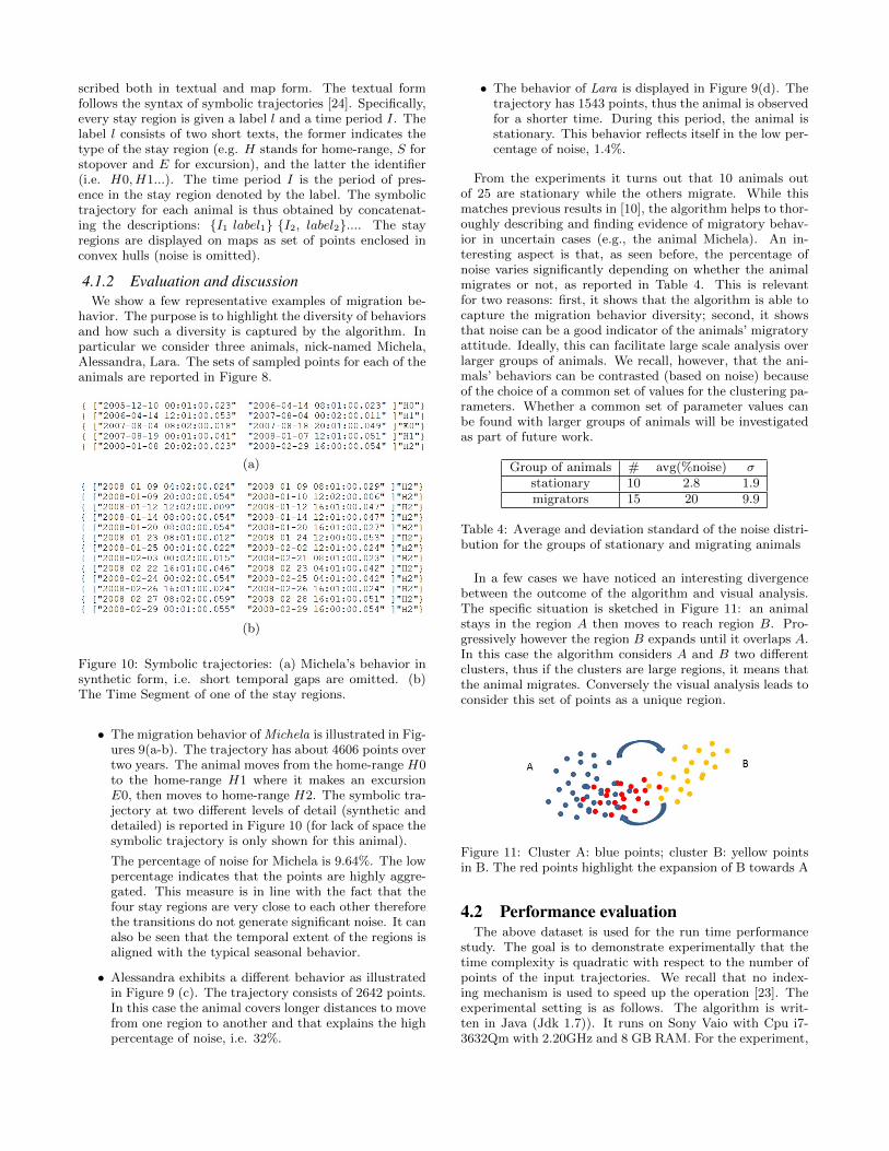
scribed both in textual and map form. The textual formfollows the syntax of symbolic trajectories [24]. Specifically,every stay region is given a label l and a time period I. Thelabel l consists of two short texts, the former indicates thetype of the stay region (e.g. H stands for home-range, S forstopover and E for excursion), and the latter the identifier(i.e. H0, H1...). The time period I is the period of pres-ence in the stay region denoted by the label. The symbolictrajectory for each animal is thus obtained by concatenat-ing the descriptions: {I1 label1} {I2, label2}.... The stayregions are displayed on maps as set of points enclosed inconvex hulls (noise is omitted).

4.1.2 Evaluation and discussionWe show a few representative examples of migration be-

havior. The purpose is to highlight the diversity of behaviorsand how such a diversity is captured by the algorithm. Inparticular we consider three animals, nick-named Michela,Alessandra, Lara. The sets of sampled points for each of theanimals are reported in Figure 8.

(a)

(b)

Figure 10: Symbolic trajectories: (a) Michela’s behavior insynthetic form, i.e. short temporal gaps are omitted. (b)The Time Segment of one of the stay regions.

• The migration behavior of Michela is illustrated in Fig-ures 9(a-b). The trajectory has about 4606 points overtwo years. The animal moves from the home-range H0to the home-range H1 where it makes an excursionE0, then moves to home-range H2. The symbolic tra-jectory at two different levels of detail (synthetic anddetailed) is reported in Figure 10 (for lack of space thesymbolic trajectory is only shown for this animal).

The percentage of noise for Michela is 9.64%. The lowpercentage indicates that the points are highly aggre-gated. This measure is in line with the fact that thefour stay regions are very close to each other thereforethe transitions do not generate significant noise. It canalso be seen that the temporal extent of the regions isaligned with the typical seasonal behavior.

• Alessandra exhibits a different behavior as illustratedin Figure 9 (c). The trajectory consists of 2642 points.In this case the animal covers longer distances to movefrom one region to another and that explains the highpercentage of noise, i.e. 32%.

• The behavior of Lara is displayed in Figure 9(d). Thetrajectory has 1543 points, thus the animal is observedfor a shorter time. During this period, the animal isstationary. This behavior reflects itself in the low per-centage of noise, 1.4%.

From the experiments it turns out that 10 animals outof 25 are stationary while the others migrate. While thismatches previous results in [10], the algorithm helps to thor-oughly describing and finding evidence of migratory behav-ior in uncertain cases (e.g., the animal Michela). An in-teresting aspect is that, as seen before, the percentage ofnoise varies significantly depending on whether the animalmigrates or not, as reported in Table 4. This is relevantfor two reasons: first, it shows that the algorithm is able tocapture the migration behavior diversity; second, it showsthat noise can be a good indicator of the animals’ migratoryattitude. Ideally, this can facilitate large scale analysis overlarger groups of animals. We recall, however, that the ani-mals’ behaviors can be contrasted (based on noise) becauseof the choice of a common set of values for the clustering pa-rameters. Whether a common set of parameter values canbe found with larger groups of animals will be investigatedas part of future work.

Group of animals # avg(%noise) σstationary 10 2.8 1.9migrators 15 20 9.9

Table 4: Average and deviation standard of the noise distri-bution for the groups of stationary and migrating animals

In a few cases we have noticed an interesting divergencebetween the outcome of the algorithm and visual analysis.The specific situation is sketched in Figure 11: an animalstays in the region A then moves to reach region B. Pro-gressively however the region B expands until it overlaps A.In this case the algorithm considers A and B two differentclusters, thus if the clusters are large regions, it means thatthe animal migrates. Conversely the visual analysis leads toconsider this set of points as a unique region.

Figure 11: Cluster A: blue points; cluster B: yellow pointsin B. The red points highlight the expansion of B towards A

4.2 Performance evaluationThe above dataset is used for the run time performance

study. The goal is to demonstrate experimentally that thetime complexity is quadratic with respect to the number ofpoints of the input trajectories. We recall that no index-ing mechanism is used to speed up the operation [23]. Theexperimental setting is as follows. The algorithm is writ-ten in Java (Jdk 1.7)). It runs on Sony Vaio with Cpu i7-3632Qm with 2.20GHz and 8 GB RAM. For the experiment,

Figure 8: Sampled points for the example animals Michela, Alessandra, Lara (QGIS maps)

(a) (b)

(c) (d)

Figure 9: (a-b)Migration pattern of Michela: from H0 to H1; and from H1 to H2. (c)Alessandra: the animal covers longerdistances. (d)Lara: stationary animal

Figure 12: Run-time performance over the dataset

we use the previous trajectory data set, extended with syn-thetic data. The purpose of synthetic data is to allow thegeneration of trajectories of arbitrary length. In particu-lar, the additional points are simply obtained by modify-ing the time-stamp, i.e. tm=tm−1 + 4h + random whererandom ∈ [−2h, 2h]. We consider the value of n rangingfrom 1000 to 10000 points for the 25 trajectories. For each

value of n, the minimum, maximum and average run time iscomputed for the 25 trajectories. The resulting graph thatconfirms the complexity analysis is shown in Figure 12.

5. RELATED WORKThe SeqScan algorithm relates to diverse density-based

clustering models. A major one is incremental clustering. Inparticular, our work takes inspiration from IncrementalDB-SCAN [19], a solution drawn to update existing DBSCANclusters. We apply a similar approach, namely the dense re-gions are progressively updated, however the updating strat-egy is different. ST-DBSCAN is an extension of DBSCANfor the clustering of events located in space and time [25]. Inaddition to the spatial neighborhood radius, ST-DBSCANconsiders a temporal neighborhood radius. Thus, a point isconsidered as core when the number of points in the neigh-borhood is greater or equal to the threshold value withinspatial and temporal thresholds. By contrast, in SeqScanthe neighborhood has exclusively a spatial meaning becauseany assumption on how space and time are related would bearbitrary. Temporal thresholds are also used for the detec-

tion of stops in high-sampling-rate trajectories [13, 22]. Thetemporal threshold in [13] specifies the minimum durationof the stop (we recall that duration is different from the con-cept of presence). The technique, however, does not provideguarantees that subsequent stops are temporally disjoint.This pitfall is avoided in [22]. However, also in this case theneighborhood consists of points that are close in space andtime, while we recall that the temporal closeness of pointsis not required in our model. A common deficiency of thesemethods is the lack of validation on real applications.

6. CONCLUSIONThe paper presents a novel framework for the study of mi-

gratory behaviors, consisting of: a mobility pattern model;an algorithm, i.e. SeqScan, to extract such a pattern fromGPS trajectories; a usage methodology for the study of wildanimal migrations; and a first validation of the whole frame-work over a real data set. On the algorithmic side, SeqScanprovides a conceptually clean and founded mechanism forthe analysis of stop-and-move like patterns over large tem-poral scales. Further properties, such as scalability issues,will be analyzed in more detail in the near future. On theapplication side, we plan to extend the use of the proposedapproach in the context of animal movement, e.g. to severalspecies/populations. This is especially valuable in the lightof recent considerations on the plasticity of animal behavior(the stationarity-migratory continuum). The use of the per-centage of noise as a quantitative index of ”migratoriness”is especially interesting and innovative, offering the oppor-tunity to fine-tune the space-time granularity at which ana-lyzing movement patterns. This also opens up the study ofhuman mobility over large temporal scales.

7. REFERENCES[1] C. Parent, S. Spaccapietra, C. Renso, G. Andrienko,

N. Andrienko, V. Bogorny, M.L. Damiani,A. Gkoulalas-Divanis, J. Macedo, N. Pelekis,Y. Theodoridis, and Z. Yan. Semantic trajectoriesmodeling and analysis. ACM Comput. Surv.,45(4):42:1–42:32, 2013.

[2] J. Gudmundsson, P. Laube, and T. Wolle. Movementpatterns in spatio-temporal data. In Encyclopedia ofGIS, pages 726–732. Springer US, 2008.

[3] Y. Zheng, L. Zhang, X. Xie, and W. Ma. Mininginteresting locations and travel sequences from gpstrajectories. In Proc. WWW, 2009.

[4] S. Dodge, R. Weibel, and A-K Lautenschutz. Towardsa taxonomy of movement patterns. InformationVisualization, 7(3-4):240–252, 2008.

[5] F. Cagnacci, L. Boitani, R. Powell, and M. Boyce.Animal ecology meets gps-based radio telemetry: aperfect storm of opportunities and challenges. Phil.Trans. R. Soc. B, 365:2157–2162, 2010.

[6] B. Chapman, C. Bronmark, J-A. Nilsson, and L.A.Hansson. The ecology and evolution of partialmigration. OIKOS, (120)12:1764–1775, 2011.

[7] S. Spaccapietra, C. Parent, M.L. Damiani, J.A.de Macedo, F. Porto, and C. Vangenot. A conceptualview on trajectories. Data Knowl. Eng.,65(1):126–146, 2008.

[8] W. H. Burt. Territoriality and home range concepts asapplied to mammals. Journal of Mammalogy,

24:346–352, 1943.

[9] J.G. Kie, J. Matthiopoulos, J. Fieberg, R.A. Powell,F. Cagnacci, M.S. Mitchell, J-M. Gaillard, and P.R.Moorcroft. The home-range concept: are traditionalestimators still relevant with modern telemetrytechnology? Philos Trans R Soc Lond B Biol Sci.,365:2221–2231, 2010.

[10] F. Cagnacci, S. Focardi, M. Heurich, and al. Partialmigration in roe deer: migratory and resident tacticsare end points of a behavioural gradient determined byecological factors. OIKOS, 120 -12:1790–1802, 2011.

[11] X. Cao, G. Cong, and C. S. Jensen. Mining significantsemantic locations from gps data. Proc. VLDBEndow., 3(1-2):1009–1020, 2010.

[12] M. Buchin, A. Driemel, M. van Kreveld, andV. Sacrist. Segmenting trajectories: A framework andalgorithms using spatiotemporal criteria. Journal ofSpatial Information Science, 3:630–660, 2011.

[13] Z. Yan and D. Chakraborty. Semantics in MobileSensing. MorganClaypool, 2014.

[14] L.O. Alvares, V. Bogorny, B. Kuijpers, J. de Macedo,B. Moelans, and A. Vaisman. A model for enrichingtrajectories with semantic geographical information.In Proc. ACM GIS, 2007.

[15] H. Yoon and C. Shahabi. Robust time-referencedsegmentation of moving object trajectories. In Proc.ICDM, 2008.

[16] A. Anagnostopoulos, M. Vlachos, M. Hadjieleftheriou,E. Keogh, and P. Yu. Global distance-basedsegmentation of trajectories. In Proc. of ACMSIGKDD, 2006.

[17] M. Buchin, H. Kruckenberg, and A.Kolzsch.Segmenting trajectories based on movement states. InProc. SDH, 2012.

[18] M. Ester, H.P. Kriegel, J. Sander, and X. Xu. Adensity-based algorithm for discovering clusters inlarge spatial databases with noise. In KDD, 1996.

[19] M. Ester, H.P. Kriegel, J. Sander, M. Wimmer, andX. Xu. Incremental clustering for mining in a datawarehousing environment. In Proc. of VLDB, 1998.

[20] F. Cao, M. Ester, W. Qian, and A. Zhou.Density-based clustering over an evolving data streamwith noise. In SDM, 2006.

[21] M. Ankerst, M. Breunig, H.P. Kriegel, and J. Sander.Optics: Ordering points to identify the clusteringstructure. In Proc. of the 1999 ACM SIGMOD, 1999.

[22] M. Zimmermann, T. Kirste, and M. Spiliopoulou.Finding stops in error-prone trajectories of movingobjects with time-based clustering. In IntelligentInteractive Assistance and Mobile MultimediaComputing, volume 53, pages 275–286. 2009.

[23] J. Sander, M. Ester, H.P. Kriegel, and X. Xu.Density-Based Clustering in Spatial Databases: TheAlgorithm GDBSCAN and Its Applications. DataMining and Knowledge Discovery, 2(2):169–194, 1998.

[24] F. Valdes, M.L. Damiani, and R.H. Guting. SymbolicTrajectories in Secondo: Pattern Matching andRewriting. In DASFAA, 2013.

[25] D. Birant and A. Kut. ST-DBSCAN: An Algorithmfor Clustering Spatial-temporal Data. Data Knowl.Eng., 60(1):208–221, 2007.