Embed Size (px)
Citation preview
Extracting Motion Primitives from Natural
Handwriting Data
Ben H Williams
TH
E
U N I V E RS
IT
Y
OF
ED I N B U
RG
H
Doctor of Philosophy
Institute for Adaptive and Neural Computation
School of Informatics
University of Edinburgh
2008

Abstract
Humans and animals can plan and execute movements much more adaptably and
reliably than current computers can calculate robotic limb trajectories. Over re-
cent decades, it has been suggested that our brains usemotor primitivesas blocks
to build up movements. In broad terms a primitive is a segment of pre-optimised
movement allowing a simplified movement planning solution. This thesis explores
a generative model of handwriting based upon the concept of motor primitives.
Unlike most primitive extraction studies, the primitives here are time extended
blocks that are superimposed with character specific offsets to create a pen trajec-
tory. This thesis shows how handwriting can be represented using a simple fixed
function superposition model, where the variation in the handwriting arises from
timing variation in the onset of the functions. Furthermore, it is shown how hand-
writing style variations could be due to primitive function differences between in-
dividuals, and how the timing code could provide a style invariant representation
of the handwriting. The spike timing representation of the pen movements pro-
vides an extremely compact code, which could resemble internal spiking neural
representations in the brain. The model proposes an novel way to infer primitives
in data, and the proposed formalised probabilistic model allows informative pri-
ors to be introduced providing a more accurate inference of primitive shape and
timing.
iii

Acknowledgements
Many thanks to my first and second supervisors, respectively Amos Storkey, and Marc
Toussaint, without whom this research would not have taken course.
Thanks go also to Chris Williams for providing helpful feedback and comments on
the research, and suggesting related material.
Financial support was gratefully received from the EPSRC and MRC, which jointly
fund the Neuroinformatics Doctoral Training Centre within the School of Informatics,
and support several post graduate students each year.
Finally, thanks go to my parents for financial and moral support, and moreover to
Val Williams for proof-reading this work.
iv

Declaration
I declare that this thesis was composed by myself, that the work contained herein is
my own except where explicitly stated otherwise in the text, and that this work has not
been submitted for any other degree or professional qualification except as specified.
(Ben H Williams
)
v


Table of Contents
1 Introduction 1
1.1 Problem statement . . . . . . . . . . . . . . . . . . . . . . . . . . . 2
1.2 Model overview . . . . . . . . . . . . . . . . . . . . . . . . . . . . . 3
1.3 Chapter overview . . . . . . . . . . . . . . . . . . . . . . . . . . . . 3
2 Background 5
2.1 Motor primitives . . . . . . . . . . . . . . . . . . . . . . . . . . . . 6
2.1.1 Electrophysiological evidence . . . . . . . . . . . . . . . . . 6
2.1.2 Psychophysical evidence . . . . . . . . . . . . . . . . . . . . 7
2.2 Modelling primitives . . . . . . . . . . . . . . . . . . . . . . . . . . 9
2.2.1 A piano model of primitives . . . . . . . . . . . . . . . . . . 11
2.3 Handwriting . . . . . . . . . . . . . . . . . . . . . . . . . . . . . . . 11
2.4 Probabilistic time series models . . . . . . . . . . . . . . . . . . . . 13
2.5 Placement and contrasts . . . . . . . . . . . . . . . . . . . . . . . . . 14
3 Assumptions and model overview 17
3.1 Biological primitives . . . . . . . . . . . . . . . . . . . . . . . . . . 17
3.2 Modelling primitives . . . . . . . . . . . . . . . . . . . . . . . . . . 18
3.3 Assumptions . . . . . . . . . . . . . . . . . . . . . . . . . . . . . . 19
3.4 Piano Model . . . . . . . . . . . . . . . . . . . . . . . . . . . . . . . 19
3.5 Probabilistic model overview . . . . . . . . . . . . . . . . . . . . . . 20
3.6 Definitions . . . . . . . . . . . . . . . . . . . . . . . . . . . . . . . . 21
3.7 Operational overview . . . . . . . . . . . . . . . . . . . . . . . . . . 26
4 Factorial Hidden Markov Model 29
4.1 Probabilistic Implementation of the Piano Model . . . . . . . . . . . 29
4.1.1 Factorial Hidden States . . . . . . . . . . . . . . . . . . . . . 30
4.1.2 Markov Properties . . . . . . . . . . . . . . . . . . . . . . . 32
vii
4.2 Model Definition . . . . . . . . . . . . . . . . . . . . . . . . . . . . 33
4.2.1 Free parameters . . . . . . . . . . . . . . . . . . . . . . . . . 37
4.3 Inference . . . . . . . . . . . . . . . . . . . . . . . . . . . . . . . . 37
4.3.1 Expectation Step . . . . . . . . . . . . . . . . . . . . . . . . 38
4.3.2 Likelihood calculation . . . . . . . . . . . . . . . . . . . . . 39
4.3.3 Maximisation Step . . . . . . . . . . . . . . . . . . . . . . . 40
4.4 Constraints and modifications . . . . . . . . . . . . . . . . . . . . . . 40
4.4.1 Modelling constraints . . . . . . . . . . . . . . . . . . . . . 41
4.4.2 Heuristic optimisations . . . . . . . . . . . . . . . . . . . . . 42
4.5 Parameter Initialisations . . . . . . . . . . . . . . . . . . . . . . . . 46
5 Factorial Hidden Markov Model Results 49
5.1 Data . . . . . . . . . . . . . . . . . . . . . . . . . . . . . . . . . . . 49
5.1.1 Datasets Used . . . . . . . . . . . . . . . . . . . . . . . . . . 54
5.2 Variance profiles of data . . . . . . . . . . . . . . . . . . . . . . . . 57
5.3 Primitives extracted . . . . . . . . . . . . . . . . . . . . . . . . . . . 57
5.4 Repeatability . . . . . . . . . . . . . . . . . . . . . . . . . . . . . . 60
5.5 Generalisation of primitives . . . . . . . . . . . . . . . . . . . . . . . 70
5.6 Character reconstructions and model robustness . . . . . . . . . . . . 76
5.7 Spike timing . . . . . . . . . . . . . . . . . . . . . . . . . . . . . . . 77
5.7.1 Generative sampling . . . . . . . . . . . . . . . . . . . . . . 77
6 Timing Model 79
6.1 Primitive-onset representation of the data . . . . . . . . . . . . . . . 79
6.2 Potential timing models . . . . . . . . . . . . . . . . . . . . . . . . . 82
6.2.1 Independent spiking model . . . . . . . . . . . . . . . . . . . 82
6.2.2 Gaussian model . . . . . . . . . . . . . . . . . . . . . . . . . 83
6.2.3 Integrate and Fire model . . . . . . . . . . . . . . . . . . . . 86
6.2.4 HMM Timing model . . . . . . . . . . . . . . . . . . . . . . 87
6.2.5 Combined hidden state HMM . . . . . . . . . . . . . . . . . 94
6.2.6 Single combined HMM . . . . . . . . . . . . . . . . . . . . 97
6.3 Generative comparison . . . . . . . . . . . . . . . . . . . . . . . . . 101
6.4 Timing constraints . . . . . . . . . . . . . . . . . . . . . . . . . . . 102
7 Coupled Model 109
7.1 Coupling method . . . . . . . . . . . . . . . . . . . . . . . . . . . . 110
viii

7.2 Generative sampling . . . . . . . . . . . . . . . . . . . . . . . . . . 113
7.3 Inference . . . . . . . . . . . . . . . . . . . . . . . . . . . . . . . . 115
7.3.1 Inference order . . . . . . . . . . . . . . . . . . . . . . . . . 115
7.3.2 Primitive fHMM inference . . . . . . . . . . . . . . . . . . . 116
7.3.3 Timing HMM inference . . . . . . . . . . . . . . . . . . . . 117
7.4 Results of coupling . . . . . . . . . . . . . . . . . . . . . . . . . . . 117
7.5 Number of primitives . . . . . . . . . . . . . . . . . . . . . . . . . . 120
8 Results 129
8.1 Generative results . . . . . . . . . . . . . . . . . . . . . . . . . . . . 129
8.1.1 Readability . . . . . . . . . . . . . . . . . . . . . . . . . . . 130
8.2 Objective measures . . . . . . . . . . . . . . . . . . . . . . . . . . . 134
8.3 Primitive swapping . . . . . . . . . . . . . . . . . . . . . . . . . . . 140
8.4 Recognition . . . . . . . . . . . . . . . . . . . . . . . . . . . . . . . 143
8.4.1 Character recognition . . . . . . . . . . . . . . . . . . . . . . 145
8.5 Comparison with other models . . . . . . . . . . . . . . . . . . . . . 148
8.5.1 Objective measures . . . . . . . . . . . . . . . . . . . . . . . 148
8.5.2 Alternative models . . . . . . . . . . . . . . . . . . . . . . . 150
8.5.3 Conclusion . . . . . . . . . . . . . . . . . . . . . . . . . . . 164
9 Discussion 167
9.1 Implications for biology . . . . . . . . . . . . . . . . . . . . . . . . 167
9.2 Implications for robotics . . . . . . . . . . . . . . . . . . . . . . . . 168
9.3 Implications for data representation . . . . . . . . . . . . . . . . . . 169
9.4 Limitations/Extensions of the model . . . . . . . . . . . . . . . . . . 170
9.4.1 Psychophysical experiments . . . . . . . . . . . . . . . . . . 173
9.5 Summary . . . . . . . . . . . . . . . . . . . . . . . . . . . . . . . . 174
10 Appendix 177
10.1 Variational Log Likelihood . . . . . . . . . . . . . . . . . . . . . . . 177
10.1.1 Regularised VLL . . . . . . . . . . . . . . . . . . . . . . . . 180
Bibliography 183
ix

Chapter 1
Introduction
This project aims to draw from two large areas of current research to form a prob-
abilistic model of handwriting, based upon the biological/robotics concept of motor
primitives.
Recently there have been many biological studies looking at how our brains plan
and control movement. These can be broken down into electrophysiological studies
(Section 2.1.1) on various animal models, and psychophysical studies (Section 2.1.2)
performed on human subjects. Almost all of these studies focus on reaching and grasp-
ing tasks, or more general limb extension tasks.
In the domain of data modelling, there have been several recent models of hand-
writing, mostly prompted by the invention and popularity of hand held personal organ-
isers incorporating digitisation tablets for input. Most of these models use some form
of modularisation, requiring a pre-segmentation of handwriting which influences the
model, and can often be unreliable. This project proposes a primitive based model that
modularises handwriting without requiring pre-segmentation.
Handwriting is an almost universal form of human communication which, before
the invention of printing, was a unique skill that allowed ideas and experience to be
passed on in a much more reliable format than with speech. Reading and writing other
people’s handwriting is a difficult task for computers and in some cases for humans as
well. This is mostly due to different styles of handwriting which lead to very different
markings meaning exactly the same thing. Also there is a great degree of variation in a
single person’s handwriting, which is normally attributed to noisy motor control. Au-
tomated handwriting recognition is therefore a very unreliable process, and is greatly
aided by some higher level language model, as in speech recognition. However, if the
variability in handwriting is better understood, then the low level recognition could
1

2 Chapter 1. Introduction
become more robust.
The aim of this project is to explore a model of handwriting based upon motor
primitives. Assumptions about the nature of motor primitives translate into assump-
tions about the type of variability that might be present in handwriting data.
Movement planning and control is a very difficult problem in real-world applica-
tions. Current robots have very good sensors and actuators, allowing accurate move-
ment execution, however the ability to organise complex sequences of movement is
still far superior in biological organisms, despite being encumbered with noisy sensory
feedback, and requiring control of many non-linear and variable muscles.
The advantage that biological control has is therefore likely to be due to a superior
internal representation and a more robust sequencing. There is much evidence to sug-
gest that biological movement generation is based uponmotor primitives, with discrete
muscle synergies found in frog spines, (Bizzi et al., 1995; d’Avella and Bizzi, 2005;
d’Avella et al., 2003; Bizzi et al., 2002), evidence of primitives being locally fixed
(Kargo and Giszter, 2000), and modularity in human motor learning and adaptation
(Wolpert et al., 2001; Wolpert and Kawato, 1998). Compact forms of representation
for any biologically produced data should therefore also be based upon primitive sub-
blocks.
1.1 Problem statement
Handwriting has much variability, arising from biological noise in the planning and
execution of the necessary movements to produce a character. Many muscles must be
activated in a coherent, coordinated fashion to control a complex system of joints in
order to achieve robust control of a pen. The possibility of modelling such a non-linear
system using a linear model would be very attractive if the variability in the data were
well captured. This project examines the use of a simple model of superimposed offset
functions to model pen trajectory data. The shape of the functions is not constrained
or limited to a particular set, and as such there are many parameters that need to be
learnt. This project explores the use of a probabilistic framework to infer the most
likely shapes of these functions, and their positions of occurrence.
If motor primitives can be approximated by fixed functions, at least for a specific
task, then modelling of the data is greatly simplified, and it provides a useful frame-
work for recognition tasks. This project explores whether the primitives present in
handwriting are consistent enough to be modelled by a function superposition model.
1.2. Model overview 3
Furthermore, if the primitives inferred are adequate to model handwriting data,
then the timing of these primitives could provide an abstraction of the character, or
a timing code. Examination of whether this timing code itself can be modelled and
usefully generalised across multiple character samples will provide further analysis of
the appropriateness of such a model of primitives.
1.2 Model overview
The model investigated in this project envisages handwriting data as a superposition
of sparsely activated motion primitives. This approach can intuitively be compared to
a Piano Model which has also been called a Piano roll model (Cemgil et al., 2005).
Just as piano music can approximately be modelled as a superposition of the sounds
emitted by each key, biological movement can be represented as a superposition of
pre-learnt motion primitives. This implies that the whole movement can be compactly
represented by the timing of each primitive by analogy to a score of music. The for-
mulated model presented in this project reflects these assumptions. The model can be
described on two levels, corresponding to Chapters 4 and 6, where on the lower level a
factorial Hidden Markov Model (fHMM) (see Ghahramani and Jordan (1997)) is used
to model the output as a combination of signals emitted from independent primitives,
where each primitive corresponds to a factor in the fHMM. On the higher level there
is a model for the primitive timing dependent upon character class. The same prim-
itive functions are shared across characters, only their timings differ. This model is
trained on handwriting data using an EM-algorithm and thereby infers the primitives
and the primitive timings inherent in these data. The inferred timing posterior for a spe-
cific character is a compact representation for the specific character which allows for a
good reproduction of this character using the learnt primitives. Furthermore, using the
timing model learnt on the higher level, new samples of characters can be generated
which are in the same writing style as the data, and also scribblings that exhibit local
similarity to written characters when the higher level timing control is omitted.
1.3 Chapter overview
Chapter 2 reviews scientific literature relating to the project. Chapter 3 defines how
primitives are approximated in this project, and some model variable definitions. Chap-
ters 4 and 5 provides details of the low-level primitive model, and chapter 6 examines

4 Chapter 1. Introduction
several possible timing models. Chapter 7 details how the primitive and timing models
are coupled together during learning. Chapter 8 assesses the performance of the model,
and compares it to some alternative models. Chapter 9 reviews the implications of the
project, and possible uses and extensions.

Chapter 2
Background
Simply reaching out and grasping an object is a task that we as humans generally take
for granted, and normally requires minimal conscious control. For decades the study of
human and animal movements has been the focus of much scientific interest, partially
motivated by the still comparatively poor performance of modern robotics and also by
a need to understand our own control systems, and their failings, for medical reasons.
In (Wolpert, 2007), Wolpert points out a significant contrast in the ability of com-
puters to beat humans at chess, with the inability of a robot arm to move the actual
chess pieces with as much dexterity as even a young child. (Wolpert, 2007; Wolpert
et al., 2001) have reviews of Bayesian decision theory as applied to biological motor
planning and control. The difference between playing chess theoretically, and con-
trolling a robot arm in the real world, is that all the variables are known, or at least
calculable and discrete in the chess game, whereas in the real world the knowledge
of the world is based upon noisy sensors that only partially measure a subset of the
world’s state. Additionally, the actuators (motors or muscles) have a degree of noise,
leading to unpredictable movements. Finally the world is a dynamic state, and so any
internal model of the world needs to be continually updated and revised.
There are two possible extremes of control strategies. Firstly, the traditional control
approach is to have a fast feedback loop, and some controller that acts to minimise an
error signal. This works with simple control problems, however in the real world the
feedback is too slow to be useful due to the complexity of any potential error signal
calculation. Secondly, there could be a pre-learnt repertoire of movements in which
entire task related movements are optimised and then selected by a central controller at
a given time. The problem with storing so many movements is that for any real world
situation the storage and selection capabilities become inadequate. Motor primitives
5
6 Chapter 2. Background
can be thought of as a compromise between these two extremes. They are loosely
defined as sub-blocks of muscle activation synergies that are fitted together to make up
a complete movement. Therefore, the same primitive might be used for many different
movements. Over the past decade there has been much biological evidence in support
of the existence of motor primitives.
2.1 Motor primitives
2.1.1 Electrophysiological evidence
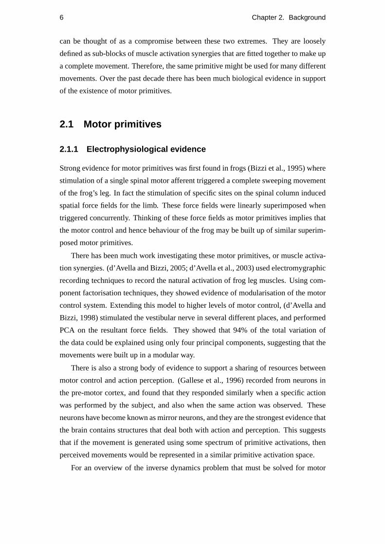
Strong evidence for motor primitives was first found in frogs (Bizzi et al., 1995) where
stimulation of a single spinal motor afferent triggered a complete sweeping movement
of the frog’s leg. In fact the stimulation of specific sites on the spinal column induced
spatial force fields for the limb. These force fields were linearly superimposed when
triggered concurrently. Thinking of these force fields as motor primitives implies that
the motor control and hence behaviour of the frog may be built up of similar superim-
posed motor primitives.
There has been much work investigating these motor primitives, or muscle activa-
tion synergies. (d’Avella and Bizzi, 2005; d’Avella et al., 2003) used electromygraphic
recording techniques to record the natural activation of frog leg muscles. Using com-
ponent factorisation techniques, they showed evidence of modularisation of the motor
control system. Extending this model to higher levels of motor control, (d’Avella and
Bizzi, 1998) stimulated the vestibular nerve in several different places, and performed
PCA on the resultant force fields. They showed that 94% of the total variation of
the data could be explained using only four principal components, suggesting that the
movements were built up in a modular way.
There is also a strong body of evidence to support a sharing of resources between
motor control and action perception. (Gallese et al., 1996) recorded from neurons in
the pre-motor cortex, and found that they responded similarly when a specific action
was performed by the subject, and also when the same action was observed. These
neurons have become known as mirror neurons, and they are the strongest evidence that
the brain contains structures that deal both with action and perception. This suggests
that if the movement is generated using some spectrum of primitive activations, then
perceived movements would be represented in a similar primitive activation space.
For an overview of the inverse dynamics problem that must be solved for motor

2.1. Motor primitives 7
planning and control, see (Mussa-Ivaldi and Bizzi, 2000). They propose a possible
solution through the use of motor primitives and an extension of the established spinal
cord basis of muscle synergies to higher motor planning areas. For a review of the
modularisation of motor control in the spine, see (Bizzi et al., 2002).
2.1.2 Psychophysical evidence
The many strategies by which humans and animals can accomplish any single motor
task in the real world have an infinite number of solutions. Despite this, we show
consistency both in varying situations, and across subjects (Todorov and Jordan, 2002;
Mataric, 2004; Wolpert et al., 2001; Wolpert and Kawato, 1998). This suggests people
use similar movement strategies. A central assumption is that such a strategy should be
in some way optimal, due to the pressures of natural selection. What exactly is being
optimised however is unclear. Wolpert has investigated this question using mostly
reaching and grasping tasks.
Wolpert’s central hypothesis, becoming increasingly accepted is that the brain uses
an approximate form of Bayesian inference to best predict what is happening in the
world, and also to plan movement in such a way as to minimise end-point position
noise in important dimensions. There must be some internal model for the purposes
of planning and prediction, and Wolpert suggests that this model is a combination of
multiple paired modules, modelling both consequence and cause (see (Wolpert and
Kawato, 1998)).
There has been much work by Wolpert and colleagues (Wolpert et al., 2001; David-
son and Wolpert, 2003, 2004; Hamilton et al., 2004; Kording et al., 2004; van Beers
et al., 2004; Witney and Wolpert, 2003; Caithness et al., 2004) looking at how our inter-
nal forward models are structured and applied in motor adaptation tasks. They suggest
that there are multiple forward and inverse internal models in the brain, and that the
movement strategies are selected so as to minimize muscle activation noise, and there-
fore end point error. For an overview of their research see (Wolpert, 2007; Wolpert
and Kawato, 1998). Their model tries to explain both motor adaptation experimental
results, and motor optimisation strategies. It has long been noted that learning differ-
ent tasks in a similar environment is more difficult than learning two unrelated tasks.
The tasks interfere with each other. However it is possible to switch motor behaviour
in different environments, for instance motor skills when playing tennis, or driving a
car. They believe that there is a modularisation of internal models, which can be in-
8 Chapter 2. Background
dependently activated for specific circumstances. This can go some way to explaining
the phenomenon of motor learning interference. Furthermore, they hypothesise that
movement strategies are evolved to minimise end-point error. This is a novel alterna-
tive to the common idea of minimising some path distance metric, such as absolute
distance, or average muscle force needed, or jerk minimisation. They have obtained
many experimental results to support this theory, which takes into account the fact that
muscle noise is proportional to muscle activation.
Wolpert’s experiments generally are concerned with reaching and grasping tasks.
Although these tasks require far larger movements than for pen-control tasks such
as handwriting, it has been suggested that a similar modelling framework could be
adapted for both types of task, for instance (Meulenbroek et al., 1996) explore the
capability for a person to write on many different scales, and even with different limbs.
During a reaching and grasping experiment, if the target is suddenly changed whilst
a movement is underway, the manner in which people are capable of reacting reveals
characteristics of the underlying system. (Kargo and Giszter, 2000) showed that rather
than simply correcting the movement, the subjects would superimpose the original
movement with another that had the effect of correction. This suggests that the prim-
itives have a time-extended and fixed component, at least once a movement has been
commenced.
The locally fixed, time-extended nature of primitives is a central assumption in this
project, and is supported by the distributed computation and representations that must
exist in the brain. If primitives are considered to be time slices, then there must be a
regular and very fast clock signal in the brain. There is no evidence to support this, and
therefore it is much more likely that primitives are ‘triggered’ at specific times, and
then are active for an extended time period, probably overlapping with several other
primitives for complex and adaptable movements.
The hypothesis that complete movements are made up of superimposed, time ex-
tended blocks of movement implies that somewhere, there must be a timing circuit
that ‘fires’ the appropriate primitive at the appropriate point. There is evidence that
the cerebellum is involved with motor function, and more specifically with timing of
motor function, and perception. (Meegan et al., 2000) showed that perceptual learning
of rhythms improved performance in motor tasks which involved the learned rhythm.
(Dennis et al., 2004) showed a relationship between cerebellar volume in children and
performance in motor timing tasks. (Penhume et al., 1998) used PET imaging to show
that the cerebellum provides a supramodal contribution to motor timing tasks. They
2.2. Modelling primitives 9
hypothesise that the cerebellum provides the necessary circuitry to extract timing in-
formation for the sensory and motor system.
If movements are repeatably composed of locally fixed sub-blocks, then with enough
samples of movement, it should be possible to infer what these sub-blocks might be,
and thus extract the primitives from data.
2.2 Modelling primitives
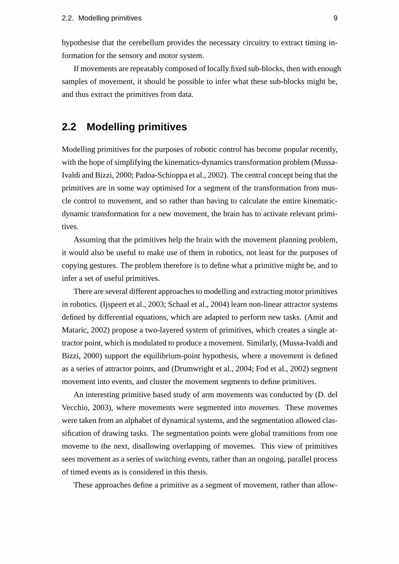
Modelling primitives for the purposes of robotic control has become popular recently,
with the hope of simplifying the kinematics-dynamics transformation problem (Mussa-
Ivaldi and Bizzi, 2000; Padoa-Schioppa et al., 2002). The central concept being that the
primitives are in some way optimised for a segment of the transformation from mus-
cle control to movement, and so rather than having to calculate the entire kinematic-
dynamic transformation for a new movement, the brain has to activate relevant primi-
tives.
Assuming that the primitives help the brain with the movement planning problem,
it would also be useful to make use of them in robotics, not least for the purposes of
copying gestures. The problem therefore is to define what a primitive might be, and to
infer a set of useful primitives.
There are several different approaches to modelling and extracting motor primitives
in robotics. (Ijspeert et al., 2003; Schaal et al., 2004) learn non-linear attractor systems
defined by differential equations, which are adapted to perform new tasks. (Amit and
Mataric, 2002) propose a two-layered system of primitives, which creates a single at-
tractor point, which is modulated to produce a movement. Similarly, (Mussa-Ivaldi and
Bizzi, 2000) support the equilibrium-point hypothesis, where a movement is defined
as a series of attractor points, and (Drumwright et al., 2004; Fod et al., 2002) segment
movement into events, and cluster the movement segments to define primitives.
An interesting primitive based study of arm movements was conducted by (D. del
Vecchio, 2003), where movements were segmented intomovemes. These movemes
were taken from an alphabet of dynamical systems, and the segmentation allowed clas-
sification of drawing tasks. The segmentation points were global transitions from one
moveme to the next, disallowing overlapping of movemes. This view of primitives
sees movement as a series of switching events, rather than an ongoing, parallel process
of timed events as is considered in this thesis.
These approaches define a primitive as a segment of movement, rather than allow-
10 Chapter 2. Background
ing a movement to be built up by multiple over-lapping primitives. The primitives
are generally assumed to be active either for the entire movement, or between pre-
segmented intervals. In real world tasks, the variety of movements that is required
is enormous, and each movement does not have a clear starting point, but follows on
fluidly from the last. This suggests that the primitive sub-blocks making up the move-
ment can probably be superimposed. This is supported by (Bizzi et al., 2002) which
suggests that the primitives in a frog’s spine when activated in combination produce
a force field that is a linear superposition of the force fields produced by the separate
primitives.
A related area to limb control is robotic navigation, and the force field summation
principle of limb control proposed in Bizzi’s work can also be found in navigation stud-
ies such as (S.R. Lindemann, 2005). There are some differences between the problems
of limb control and navigation, such as the constraints on the task. In general naviga-
tion constraints relate to obstacle avoidance, whereas limb control is more concerned
with speed, accuracy of path, and in particular accuracy of end point position. However
it is interesting to note that a similar model can be used for both tasks. Primitive based
navigation policies can also be found, such as (D.C. Conner, 2006), where sequentially
composed movements are constructed using switching of local feedback control poli-
cies. Similarly to (D. del Vecchio, 2003), there is no overlapping of the policies, thus
the movements are segmented by global switching points. This implies a single central
synchronous controller rather than large parallel operation of multiple asynchronous
controlling elements, as is likely to be the case in the brain. Most robotics studies con-
sider primitives in such a fashion, effectively as a method of segmenting movements.
This thesis considers primitives to be individually segmented into their onset times, but
independent from each other and without any global switching of primitives.
Pre-segmentation followed by PCA/ICA is often used to extract components that
are referred to as primitives (Fod et al., 2002). These primitives are therefore strongly
defined by the segmentation points within the movement. For certain movements with
clearly defined start points, this technique is effective for movement classification,
mainly due to the speed of ICA algorithms. For a review of ICA techniques, see
(Hyvarinen, 1999), and an interesting extension to ICA is proposed by (Karklin and
Lewicki, 2005) focussing on image patches. However in the real world, movements
cannot be segmented into start points, and so using a windowed technique is difficult.
2.3. Handwriting 11
2.2.1 A piano model of primitives
Assuming that the primitives can overlap, that they have no common start point and
that they cannot be instantly switched off, there is an analogous model that is used in
music. A simple piano can be modelled as a series of key presses at different times.
These key presses give rise to sound waves which are overlaid to create the music that
the audience hear. (Cemgil et al., 2005) name such a model a ‘piano-roll’ model, due
to its similarities with the pianola or reproducing piano. The idea of this analogy is to
use such a model to inferwhichnotes are being playedwhenin a piece of music. This
model is further discussed in Chapter 3.
Assuming the data is made up of time-extended functions with specific offsets, one
way to extract them is by using a pattern extraction algorithm. (Chiu et al., 2003)
propose an efficient algorithm that finds recurrent patterns within a time series. This
model uses tolerance levels to determine how similar the data must be to define a motif,
rather than formally modelling noise in the data. If several motifs are superimposed
with different offsets, it is uncertain how successful such a pattern-matching based
approach would be in reconstructing the original separate motifs.
The offset function model is also attractive for auditory encoding, as is suggested
in (Lewicki and Sejnowski, 1999; Smith and Lewicki, 2005). Although they are not
trying to model motor primitives, the concept is similar to the piano model proposed in
Chapter 3. A sound wave can be decomposed into a set of basis functions with various
offsets. Once a reasonable reconstruction is obtained, the basis can be adapted to better
represent the signal, thus effectively extracting primitives from the signal. More details
and a comparison with this model can be found in Section 8.5.2.3.
2.3 Handwriting
Handwriting is an extremely useful skill that has revolutionised human communication
over the past 6000 years, allowing ideas and discoveries to be communicated more pre-
cisely and repeatably than by spoken word. Evolutionarily speaking, it is a relatively
new motor skill, as compared to walking, grabbing, or even speech. These older skills
are likely to have evolved a specialised brain area over a longer period of time, while
handwriting is probably controlled by a generalised motor planning area in the brain,
responsible for generic adaptable behaviour. The biological control of handwriting,
despite its enormous importance, and high symbolic information content is probably
12 Chapter 2. Background
treated similarly to any another hand movement by the brain. Handwriting was chosen
as the dataset to model for this reason, and because it is now easy to get very accurate
pen trajectory data from digitisation tablets.
Most handwriting studies over the past three decades have been focussed entirely
on recognition. For a review of handwriting recognition see (Meulenbroek and Gem-
mert, 2003; Beigi, 1993). Handwriting and more general movement studies have found
a consistent relationship between angular velocity and curvature of movements, known
as the two-thirds law. This is explored in a novel way by (T. Flash, 2007) who propose
that this relationship is due to a non-Euclidean internal geometrical representation of
space. They show how successive application of geometrical transformations can be
used to construct movements. It would be interesting to examine whether geomet-
rical primitives could be used to produce movements that have similar properties as
biologically produced movements.
An inverse dynamics approach to handwriting was explored by (Singer and Tishby,
1994), in which cursive handwriting was treated as a system of oscillators, which could
be modulated to create characters. This approach has similarities with the primitives
proposed by (Ijspeert et al., 2003; Schaal et al., 2004), which combine oscillatory and
transient primitives.
An interesting framework for modelling handwriting was proposed by (Hinton and
Nair, 2005), which uses a spring system to model the pen dynamics, where the stiffness
of the springs over time dictates what character is being written. Inference of a motor
program is done for a single character image, and then noise is added to the image and
the motor program in such a way as to train a neural network to learn the distribution
over motor programs that can create such an image. With a few additional algorithmic
features, a good recognition performance is obtained.
Examination of human learning of handwriting can potentially reveal aspects of
the internal representation. (Marquardt et al., 1999) support the idea of primitives
in handwriting by varying the visual feedback. They find that varying the size of
characters will produce an adaptation in the handwriting only after the first character
written. In a second experiment they vary a target during a handwriting stroke, and
find that rather than aborting the initial movement, a second stroke is added. This is
similar to the findings of (Kargo and Giszter, 2000) where the experiment is a reaching
and grasping task.
(Kharraz-Tavakol et al., 2000) found that when learning two new but similar char-
acters, there is a significant transfer in learning between the two characters. This
2.4. Probabilistic time series models 13
supports the idea of subroutines being involved in character production, rather than
learning a distinct motor program for each character.
An alternative to PCA/ICA decomposition of handwriting is proposed by (Ramsay,
2000), where they use spline fitting to decompose handwriting trajectories into deriv-
ative functions. These functions are assumed to be active over the whole handwriting
sample, and the samples are linearly interpolated, and registered prior to analysis, sim-
ilarly to fixed-dimension techniques such as PCA/ICA. The argument is that any phys-
ical system must have derivatives due to Newton’s third law, and so this is a logical
way in which to decompose movements. It would be interesting to examine whether
primitives could be extracted with derivatives, or potentially a set of first derivative
primitives, and a set of second, etc. An extension to this thesis could be to include a
derivative based system in the output, and have the primitives parameterise the system.
2.4 Probabilistic time series models
If biologically produced movement data are made up of primitives, then a time series
analysis of such data should take into account the modular nature of their generation.
A common probabilistic framework for modelling time series data with hidden under-
lying structure is the Hidden Markov Model (HMM). This model, and a specialised
subset is discussed further in Chapter 4. HMM models have been used extensively
in speech recognition, mostly as language models, which provide a prior for which
characters or words are likely to come next, given the current context. Such an in-
formed prior can help recognition tasks enormously. A tutorial on HMMs and their
uses, focussing on speech recognition can be found in (Rabiner, 1989).
Also in the field of speech, (Roweis and Alwan, 1997) uses a constrained HMM
to model articulatory information in the hidden state. By constraining the hidden state
transitions to be smooth, the transformation from spectra to articulation is based upon
multiple time steps. The smooth underlying articulation trajectory could then be used
for recognition purposes.
(Vinciarelli and Bengio, 2002) use an HMM system for character recognition. A
sliding window scans across the image containing the characters, providing a feature
vector. PCA/ICA is used to de-correlate the data, before using continuous density
HMMs to model the transitions between feature vectors within a character in a word.
This system works well, and demonstrates the flexibility of HMMs, as they are not
modelling time transitions here, rather than dependencies between adjacent parts of
14 Chapter 2. Background
the image.
To create a handwriting model based upon motor primitives, a system with multi-
ple concurrent modules is required. This is similar to the piano model (Cemgil et al.,
2005), or the atomic decomposition model (Lewicki and Sejnowski, 1999; Smith and
Lewicki, 2005), which are both based upon offset, overlapping functions. A proba-
bilistic framework for modelling such situations exists as a constrained version of an
HMM. Assuming the hidden state is made up of several independent factors, the tran-
sition matrix can be split up, leading to a Factorial Hidden Markov Model (fHMM).
This subset of an HMM is discussed in detail in (Ghahramani and Jordan, 1997). In
its exact form, it is identical to a very large HMM, with a specialised transition matrix.
However the factorial nature of the hidden state allows a special variational method to
be used during inference. The main drawback of HMMs is the extent of the computa-
tional requirements for inference. Using a variational approximation such as the one
proposed in (Ghahramani and Jordan, 1997) greatly improves the speed. The fHMM
model is used as the basis for the low level primitive model in this project, and more
detail on the model and its implementation can be found in Chapter 4.
2.5 Placement and contrasts
The approach of this thesis is similar in many ways to Lewicki’s atomic signal decom-
position. The two methods are discussed and contrasted in further detail in Section
8.5.2.3. Indeed it could be argued that this thesis treats movements more like sounds,
as there are no dynamical feedback systems being modelled.
A fixed function approximation of biological primitives was chosen as an attempt
to model the variation in movements based upon an assumption of timing noise being
present in the brain. Clearly there will be other sources of variation, such as that arising
from dynamical systems. This is modelled simply as Gaussian output covariance, and
an extension to this work would be to include a dynamical system, such as the spring
system proposed by Hinton for the purposes of character production.
The offset function model was chosen here because of the assumption of asyn-
chrony and massively parallel operation of the brain. If the brain organises movement
in a parallel fashion, it can be assumed that there will be much timing noise present in
the sequencing stage. This simple noise will then give rise to complex variation in the
output due to the superposition of the many primitives. This thesis attempts to explain
the variation in handwriting in terms of timing noise within such a model. No dynam-

2.5. Placement and contrasts 15
ical system was explored so as to keep the primitives as simple as possible within the
offset model, and to examine exactly the extent that timing noise gives rise to typical
handwriting variation.
The timing code of the primitives may well be mirrored in the spiking activity of
biological brains, a similar hypothesis to Lewicki’s spikegram as a representation of
cochlear encoding. In that sense the primitives here can be thought of as biologically
inspired, however, without a model of the physical system of the hand and arm, our
primitives remain in ‘pen-space’. This is really an engineering compromise, as imple-
menting such a model would further complicate the inference procedure. This thesis
is motivated by biological studies into primitives, and hopefully provides a method in
which biological primitives may be studied, and an insight into how the brain could
be planning movement. Engineering motivations also exist, such as the possibility of
using primitives for robotic control or handwriting representation. The assumption is
that an accurate model of the biological primitives will also be a very good model for
robotic control, or in the very least, a good model for perception of biological move-
ments.
Essentially this thesis attempts to explain the variation in handwriting by finding
hidden structure in handwriting data noise, where the types of structure of this noise
are based upon biologically inspired concepts of motor primitives.


Chapter 3
Assumptions and model overview
The biological evidence for motor primitives has been discussed in Chapter 2, where a
broad spectrum of evidence indicating modularity of the motor system was presented.
This chapter formalises how we define primitives, and how we base a model of hand-
writing upon the concept of biological motor primitives.
3.1 Biological primitives
Chapter 2 discussed various studies about motor primitives in biology. The central
idea behind motor primitives is a possible simplification of the motor planning prob-
lem. This problem is that biological (and indeed robotic) bodies have many joints,
and muscles, which must be controlled in a coherent manner to perform a physical
task. The brain must output a spectrum of muscle activation commands, given a large
amount of sensory input sampling the state of the world, including the state of the body
being controlled. This sensory information is very noisy, and incomplete, whilst the
world itself is very variable and even the body being controlled is likely to have a de-
gree of unpredictability, such as muscle tiredness, muscle and limb growth, clothing,
and so on. Furthermore, the delay between muscle activation and sensory feedback is
extremely long, at least in terms of traditional control theory.
Despite all these difficulties, which become apparent when trying to control ro-
botic movement in real world environments, biological organisms perform movement
control tasks reliably and repeatably, and are also able to adapt quickly to novel envi-
ronments. The idea of motor primitives constitutes a proposed method by which the
brain may be achieving these goals. A motor primitive can be thought of as a sub-
block, or subroutine of motion, which controls a segment of the spectrum of muscle
17
18 Chapter 3. Assumptions and model overview
activations to perform a movement. The brain then has to fit these motor primitives
together in a coherent fashion, rather than calculate the appropriate levels of muscle
activation.
3.2 Modelling primitives
The exact nature of a motor primitive is unknown. Various possible definitions exist,
for instance a motor primitive can be thought of as muscle activations which generate
an end-point force field (Bizzi et al., 1995; d’Avella and Bizzi, 2005; d’Avella et al.,
2003; Bizzi et al., 2002), dynamical systems defining attractor dynamics (Ijspeert et al.,
2003; Schaal et al., 2004; Amit and Mataric, 2002), modular models of limb dynam-
ics (Wolpert et al., 2001; Wolpert and Kawato, 1998), and independent component
decomposition (Mataric, 2004).
Primitives are unlikely to be time-indexed, fixed dimensional constructs such as
those defined by an ICA analysis of data. For the brain to control such primitives,
it would need some universal clock prompting the swapping of one set of primitives
for another at each time step. Assuming that the brain operates as an asynchronous
machine, it is more likely that the primitives are time-extended blocks that define a
section of muscle activations over this time-period.
The range and adaptability of biological movement suggests that the manner in
which the primitives can be combined must be fairly flexible. Instead of having a se-
quence of primitives, it is more likely that they can be combined together, such as in
superposition. This theory is suggested in (Bizzi et al., 1995), where the concurrent ac-
tivation of primitives leads to roughly linearly superimposed force fields. It is therefore
assumed that primitives may be superimposed with non-concurrent activation.
The length of a primitive is unknown, but is assumed to be shorter than the length
of the task being performed, and could be different for different primitives. It is also
assumed that once a primitive has been initiated, it mustplay out its entire length, as
suggested by (Kargo and Giszter, 2000). Therefore instead of switching off a primi-
tive mid-length, the brain can only modify a movement mid-length by superimposing
another primitive.

3.3. Assumptions 19
3.3 Assumptions
The data being modelled in this project is generated from handwriting samples. The
data is captured as pen-tip trajectories. The primitives are modelled in the same space
as the pen-tip data, rather than trying to create a model of the physical system of the
hand and arm where primitives would consist of high dimensional muscle activations.
Primitives are assumed to be locally fixed, time-extended arbitrary functions in pen
trajectory space. These functions are superimposed with specific offsets to create the
trajectory giving rise to a particular character.
3.4 Piano Model
The model described above has been called aPiano Model(also called Piano roll
model (Cemgil et al., 2005)), due to its similarities with a simplistic model of a Piano
being played. In this model, the score contains the timing information dictating when
the notes should be played, and the music is a superposition of the waveforms over
time. The variation in the sound produced is due to variations in the timing of the
notes, rather than variations in the waveforms of the notes themselves. Such a model
can be formalised as a fixed function offset model,
y(t) =I
∑i=1
Ji
∑j=1
αi, jwi(t− τi, j) , (3.1)
wherey(t) is the observable output, which in the case of a piano is the music as heard
by a listener. In this formulation, there areI fixed functions,wi(t), which occur at
specific offsets,τi, j , and with specific scaling factors,αi, j . Each function occursJi
times within the sampley(t).
We define our primitives in the space of pen trajectories as the functionswi(t).
There are no constraints on where the primitives might occur in the characters, and
there are no constraints on the shapes of the primitives. To simplify the problem, the
scaling factors,αi, j are set to unity, thus removing them from the model.
To learn the shapes of the primitives, and the timings of the primitives in a data
sample, we assume that there is a degree of noise in both of these quantities. This
variation can be modelled in a probabilistic framework.
20 Chapter 3. Assumptions and model overview
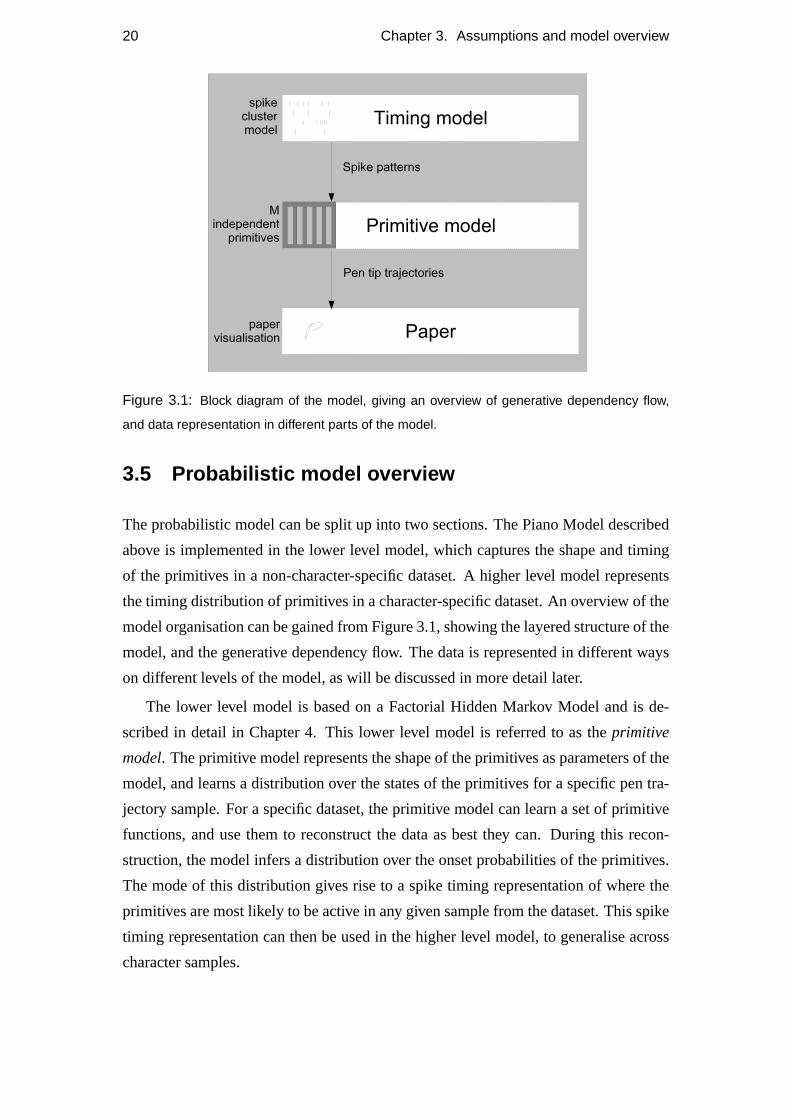
Figure 3.1: Block diagram of the model, giving an overview of generative dependency flow,
and data representation in different parts of the model.
3.5 Probabilistic model overview
The probabilistic model can be split up into two sections. The Piano Model described
above is implemented in the lower level model, which captures the shape and timing
of the primitives in a non-character-specific dataset. A higher level model represents
the timing distribution of primitives in a character-specific dataset. An overview of the
model organisation can be gained from Figure 3.1, showing the layered structure of the
model, and the generative dependency flow. The data is represented in different ways
on different levels of the model, as will be discussed in more detail later.
The lower level model is based on a Factorial Hidden Markov Model and is de-
scribed in detail in Chapter 4. This lower level model is referred to as theprimitive
model. The primitive model represents the shape of the primitives as parameters of the
model, and learns a distribution over the states of the primitives for a specific pen tra-
jectory sample. For a specific dataset, the primitive model can learn a set of primitive
functions, and use them to reconstruct the data as best they can. During this recon-
struction, the model infers a distribution over the onset probabilities of the primitives.
The mode of this distribution gives rise to a spike timing representation of where the
primitives are most likely to be active in any given sample from the dataset. This spike
timing representation can then be used in the higher level model, to generalise across
character samples.
3.6. Definitions 21
The higher level model is based on a set of Hidden Markov Models, as detailed
in Chapter 6, and referred to as thetiming model. The timing model takes the spike
timing information generated by the primitive model as the data to be modelled. It is
assumed that the spikes come from hidden Gaussian components, which can produce
at most one spike, and are not always present. The timing model captures variation
in the spike timing data, whilst providing an adequate template to produce a coherent
character sample.
The two models are coupled together by use of aspike prior, which is the prior
probability of primitive onset at any one time point, as determined by the timing model.
The method of coupling is detailed in Chapter 7. Intuitively, the primitive model learns
what the primitives look like, and where they are active in all character samples. Given
the timing of the primitives, the timing model then determines the likely timing of
primitives based upon all samples of a particular character. The prior probability of
primitive onset is then used to improve the primitive model’s inference of primitive
shape and timing.
The transformation of the trajectory data into spike timing data via the primitive
model is a strong compression of the data, and allows efficient higher level models
that generalise across character samples much faster than could be done using the un-
transformed trajectory data. This compression is the key advantage of using primitives
to represent the data, and reflects the advantage of motor primitives as a biological
movement planning tool in the brain.
3.6 Definitions
There are multiple parameter matrices in the model, and state variables. To clarify
what they are representing, an overview is presented here. There are other parameters,
such as Markov transition matrices and covariance matrices that are introduced where
appropriate in the model descriptions.
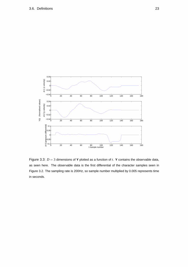
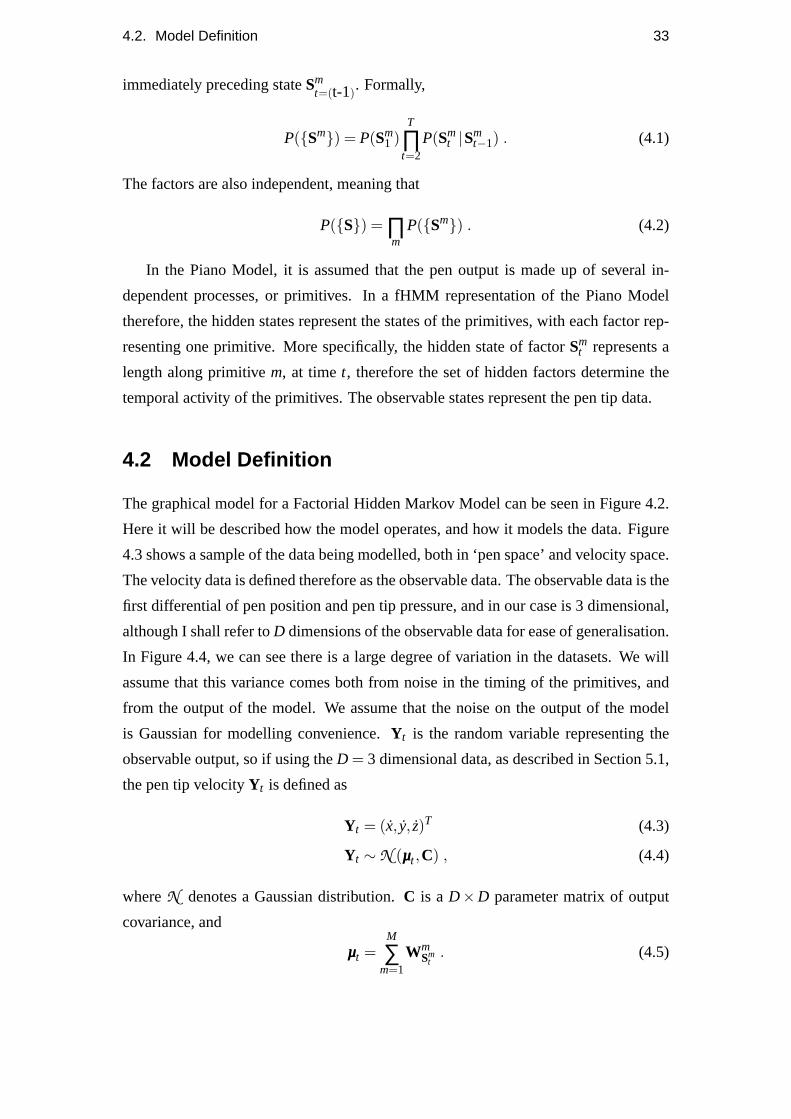
Yd,t Characters such as those seen in Figure 3.2 were collected using a digitisation
tablet. Y represents the normalised first differential of the data, which can be
seen in Figure 3.3. The differentiation was done numerically, such that
Y′t = Yt−Yt−1 . (3.2)
As the dataset is normalised, there is no need to divide by aδt. The dataset
normalisation ensures that the variance over time samples of each dimension of
22 Chapter 3. Assumptions and model overview
−5 0 5−10
−5
0
−5 0 5
−10
−5
0
−8−6−4−2 0 2−10
−5
0
−5 0 5 10−5
0
5
10
0 5 10 15
−10
−5
0
5
−15−10 −5 0−15
−10
−5
0
Dis
tanc
e /m
m
−10 −5 0 5
−15
−10
−5
0
−10 0 10
−15
−10
−5
0
0 5 10 15
−10
−5
0
5
−5 0 5 10−15
−10
−5
0
−8−6−4−2 0 2
−8−6−4−2
0
−5 0 5
−10
−5
0
−10−5 0 5−20
−10
0
−5 0 5
−10
−5
0
−10 −5 0−10
−5
0
0 5 10
−10
−5
0
0 5 10
−10
−5
0
−5 0 5 10−15
−10
−5
0
5
Distance /mm−10−5 0 5
−20
−10
0
0 5 10
−10
−5
0
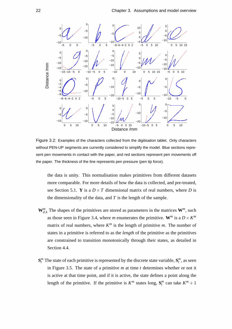
Figure 3.2: Examples of the characters collected from the digitisation tablet. Only characters
without PEN-UP segments are currently considered to simplify the model. Blue sections repre-
sent pen movements in contact with the paper, and red sections represent pen movements off
the paper. The thickness of the line represents pen pressure (pen tip force).
the data is unity. This normalisation makes primitives from different datasets
more comparable. For more details of how the data is collected, and pre-treated,
see Section 5.1.Y is aD×T dimensional matrix of real numbers, whereD is
the dimensionality of the data, andT is the length of the sample.
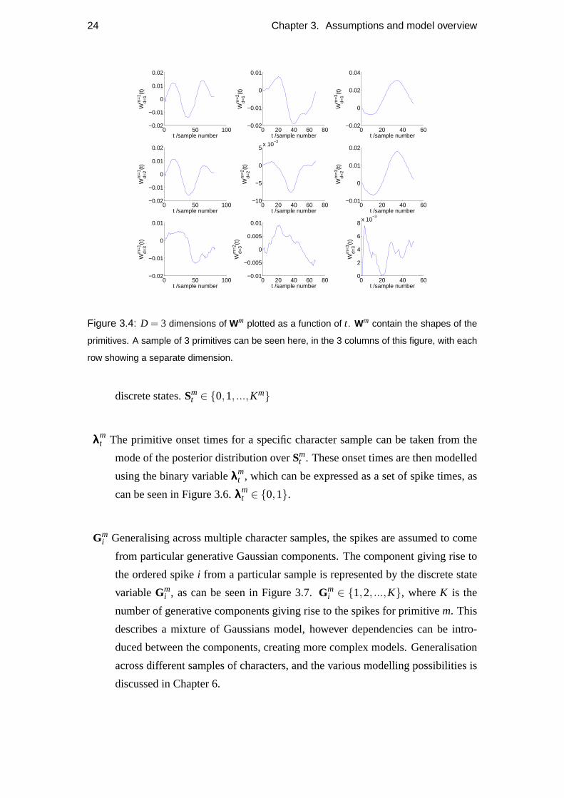
Wmd,k The shapes of the primitives are stored as parameters in the matricesWm, such
as those seen in Figure 3.4, wherem enumerates the primitive.Wm is aD×Km
matrix of real numbers, whereKm is the length of primitivem. The number of
states in a primitive is referred to as thelengthof the primitive as the primitives
are constrained to transition monotonically through their states, as detailed in
Section 4.4.
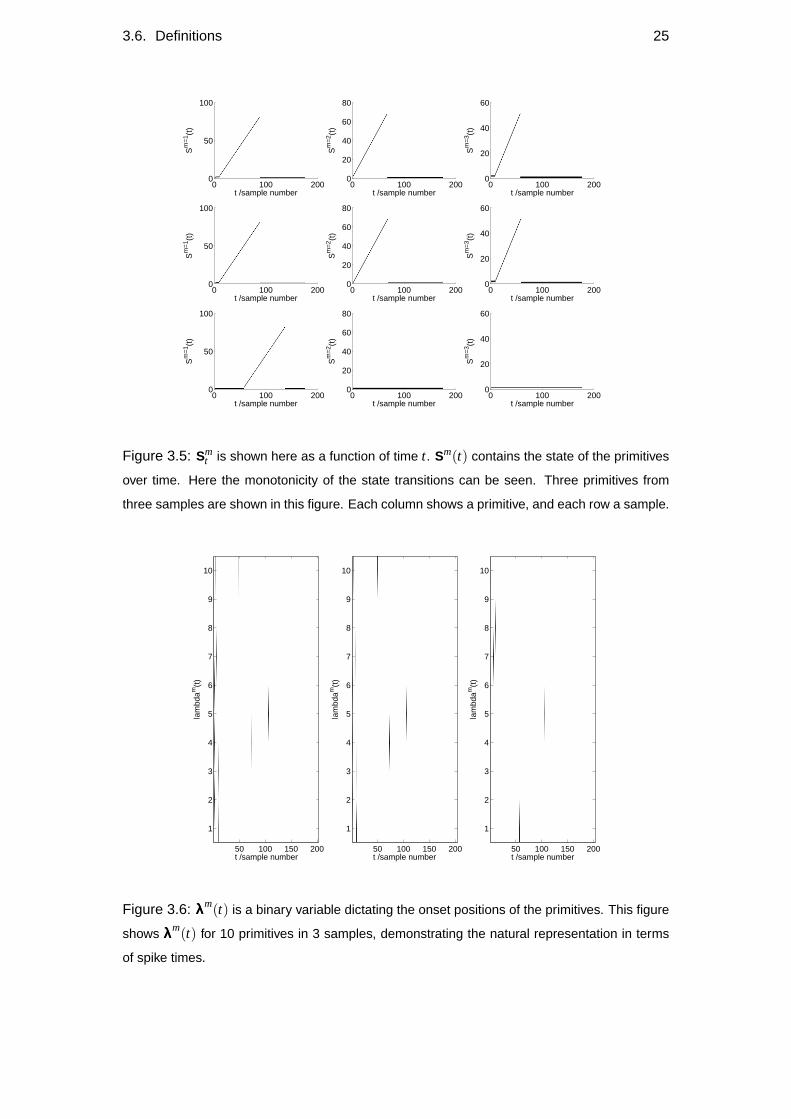
Smt The state of each primitive is represented by the discrete state variable,Sm
t , as seen
in Figure 3.5. The state of a primitivem at timet determines whether or not it
is active at that time point, and if it is active, the state defines a point along the
length of the primitive. If the primitive isKm states long,Smt can takeKm+ 1
3.6. Definitions 23
0 20 40 60 80 100 120 140 160 180−0.04
−0.02
0
0.02
0.04
d=1
(x v
eloc
ity)
0 20 40 60 80 100 120 140 160 180−0.04
−0.02
0
0.02
0.04
Y(t
) (
Nor
mal
ised
val
ues)
d=2
(y v
eloc
ity)
0 20 40 60 80 100 120 140 160 180−0.1
−0.05
0
0.05
0.1
t /sample number
d=3
(pre
ssur
e di
ffere
ntia
l)
Figure 3.3: D = 3 dimensions of Y plotted as a function of t. Y contains the observable data,
as seen here. The observable data is the first differential of the character samples seen in
Figure 3.2. The sampling rate is 200Hz, so sample number multiplied by 0.005 represents time
in seconds.
24 Chapter 3. Assumptions and model overview
0 50 100−0.02
−0.01
0
0.01
0.02
t /sample numberW
d=1
m=
1 (t)
0 20 40 60 80−0.02
−0.01
0
0.01
t /sample number
Wd=
1m
=2 (t
)
0 20 40 60−0.02
0
0.02
0.04
t /sample number
Wd=
1m
=3 (t
)
0 50 100−0.02
−0.01
0
0.01
0.02
t /sample number
Wd=
2m
=1 (t
)
0 20 40 60 80−10
−5
0
5x 10
−3
t /sample number
Wd=
2m
=2 (t
)
0 20 40 60−0.01
0
0.01
0.02
t /sample number
Wd=
2m
=3 (t
)
0 50 100−0.02
−0.01
0
0.01
t /sample number
Wd=
3m
=1 (t
)
0 20 40 60 80−0.01
−0.005
0
0.005
0.01
t /sample number
Wd=
3m
=2 (t
)
0 20 40 600
2
4
6
8x 10
−3
t /sample number
Wd=
3m
=3 (t
)
Figure 3.4: D = 3 dimensions of Wm plotted as a function of t. Wm contain the shapes of the
primitives. A sample of 3 primitives can be seen here, in the 3 columns of this figure, with each
row showing a separate dimension.
discrete states.Smt ∈ {0,1, ...,Km}
λλλmt The primitive onset times for a specific character sample can be taken from the
mode of the posterior distribution overSmt . These onset times are then modelled
using the binary variableλλλmt , which can be expressed as a set of spike times, as
can be seen in Figure 3.6.λλλmt ∈ {0,1}.
Gmi Generalising across multiple character samples, the spikes are assumed to come
from particular generative Gaussian components. The component giving rise to
the ordered spikei from a particular sample is represented by the discrete state
variableGmi , as can be seen in Figure 3.7.Gm
i ∈ {1,2, ...,K}, whereK is the
number of generative components giving rise to the spikes for primitivem. This
describes a mixture of Gaussians model, however dependencies can be intro-
duced between the components, creating more complex models. Generalisation
across different samples of characters, and the various modelling possibilities is
discussed in Chapter 6.
3.6. Definitions 25
0 100 2000
50
100
t /sample numberS
m=
1 (t)
0 100 2000
20
40
60
80
t /sample number
Sm
=2 (t
)
0 100 2000
20
40
60
t /sample number
Sm
=3 (t
)
0 100 2000
50
100
t /sample number
Sm
=1 (t
)
0 100 2000
20
40
60
80
t /sample number
Sm
=2 (t
)
0 100 2000
20
40
60
t /sample number
Sm
=3 (t
)
0 100 2000
50
100
t /sample number
Sm
=1 (t
)
0 100 2000
20
40
60
80
t /sample number
Sm
=2 (t
)
0 100 2000
20
40
60
t /sample number
Sm
=3 (t
)Figure 3.5: Sm
t is shown here as a function of time t. Sm(t) contains the state of the primitives
over time. Here the monotonicity of the state transitions can be seen. Three primitives from
three samples are shown in this figure. Each column shows a primitive, and each row a sample.
t /sample number
lam
bdam
(t)
50 100 150 200
1
2
3
4
5
6
7
8
9
10
t /sample number
lam
bdam
(t)
50 100 150 200
1
2
3
4
5
6
7
8
9
10
t /sample number
lam
bdam
(t)
50 100 150 200
1
2
3
4
5
6
7
8
9
10
Figure 3.6: λλλm(t) is a binary variable dictating the onset positions of the primitives. This figure
shows λλλm(t) for 10 primitives in 3 samples, demonstrating the natural representation in terms
of spike times.
26 Chapter 3. Assumptions and model overview
i /spike number
Gm
=1 (i)
1 2
1
2
3
4
5
i /spike number
Gm
=2 (i)
1 20.5
1
1.5
2
2.5
3
3.5
4
4.5
i /spike number
Gm
=3 (i)
1 20.5
1
1.5
2
2.5
3
3.5
i /spike number
Gm
=4 (i)
1 20.5
1
1.5
2
2.5
3
3.5
i /spike number
Gm
=5 (i)
1 2 3
1
2
3
4
5
i /spike number
Gm
=6 (i)
1 2 3
1
2
3
4
5
6
7
i /spike number
Gm
=7 (i)
1 20.5
1
1.5
2
2.5
3
3.5
4
4.5
i /spike number
Gm
=8 (i)
1 2
1
2
3
4
5
6
i /spike number
Gm
=9 (i)
0.5 1 1.5
1
2
3
4
5
6
i /spike number
Gm
=10
(i)
1 20.5
1
1.5
2
2.5
3
3.5
4
4.5
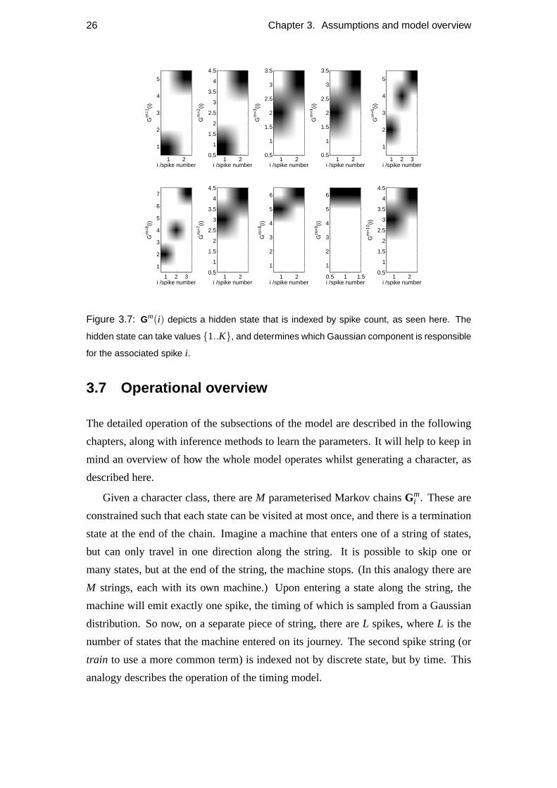
Figure 3.7: Gm(i) depicts a hidden state that is indexed by spike count, as seen here. The
hidden state can take values {1..K}, and determines which Gaussian component is responsible
for the associated spike i.
3.7 Operational overview
The detailed operation of the subsections of the model are described in the following
chapters, along with inference methods to learn the parameters. It will help to keep in
mind an overview of how the whole model operates whilst generating a character, as
described here.
Given a character class, there areM parameterised Markov chainsGmi . These are
constrained such that each state can be visited at most once, and there is a termination
state at the end of the chain. Imagine a machine that enters one of a string of states,
but can only travel in one direction along the string. It is possible to skip one or
many states, but at the end of the string, the machine stops. (In this analogy there are
M strings, each with its own machine.) Upon entering a state along the string, the
machine will emit exactly one spike, the timing of which is sampled from a Gaussian
distribution. So now, on a separate piece of string, there areL spikes, whereL is the
number of states that the machine entered on its journey. The second spike string (or
train to use a more common term) is indexed not by discrete state, but by time. This
analogy describes the operation of the timing model.

3.7. Operational overview 27
The primitive model can be thought of asM machines able to enter states onloops
of string. The size of each loop is referred to as the length of the primitive. Initially
all M machines are in a rest state on the loops (think of a knot perhaps), where they
temporarily remain. Each loop of string is associated with one of the spike trains. As
time progresses, the appearance of a spike causes the associated machine sitting in its
rest state on the loop to start progressing around the loop, at a constant speed, until the
rest state is once again reached, and the machine must wait until the next spike. As the
machine steps around the loop, it outputs a varying weight which is associated with
each state around the loop. (In the rest state, this weight is zero.) Therefore, at any
one time point, there areM machines onM loops, givingM weights. The sum of these
weights parameterises a Gaussian output distribution, describing the pen tip velocities
at each time point. Therefore sampling from this distribution at each time point gives
the complete velocity trajectory of the pen for a single character.
It should be noted at this stage that the timing model machine is indexed by spike
count, whereas the primitive model machine is indexed by time. This complicates the
inference procedure as we shall see later on, and necessitates a mixture of Gaussians
distribution to approximate the timing model for coupling purposes.

Chapter 4
Factorial Hidden Markov Model
In Chapter 3, a simple deterministic model is described, the Piano Model, where prim-
itives are defined as fixed arbitrary functions. These functions are superimposed with
time offsets, to create the output signal giving rise to the data. The data we are con-
cerned with is handwriting trajectory data, although the model could be applied to any
repeatable biologically generated data. This model is the motivation behind the com-
plete probabilistic model described in Section 3.5. The complete model was described
in a top-down fashion, to give an idea of the generative procedure. It is possible to
decouple the model into two levels, and run these stages separately. The two stages of
the model are named the Primitive model, and the Timing model. The Primitive model
can be thought of as the output, or low-level stage of the model, and the Timing model
as a higher level controlling part of the model. The Primitive model is learnt using a
Factorial Hidden Markov Model framework, as described in this chapter. The Timing
model is learnt using several Hidden Markov Models, as described in Chapter 6.
Some of the work in this chapter is published in (Williams et al., 2006), with more
detail here. In this chapter, we look at the probabilistic implementation of the Pi-
ano Model, and the correspondences and differences of the two models. We then go
through the details of the model and the method of inference, and finally the constraints
and modifications to the algorithm.
4.1 Probabilistic Implementation of the Piano Model
In Chapter 3 the motivating model was described, which was referred to as the Piano
Model. In this model, a set ofM primitives are superimposed with various offsets.
The primitives in this model are defined as fixed, time extended functions, of varying
29
30 Chapter 4. Factorial Hidden Markov Model
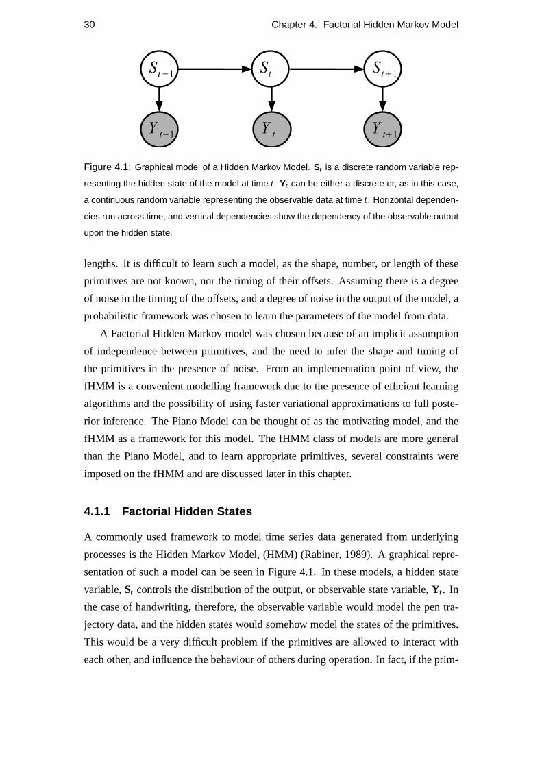
Figure 4.1: Graphical model of a Hidden Markov Model. St is a discrete random variable rep-
resenting the hidden state of the model at time t. Yt can be either a discrete or, as in this case,
a continuous random variable representing the observable data at time t. Horizontal dependen-
cies run across time, and vertical dependencies show the dependency of the observable output
upon the hidden state.
lengths. It is difficult to learn such a model, as the shape, number, or length of these
primitives are not known, nor the timing of their offsets. Assuming there is a degree
of noise in the timing of the offsets, and a degree of noise in the output of the model, a
probabilistic framework was chosen to learn the parameters of the model from data.
A Factorial Hidden Markov model was chosen because of an implicit assumption
of independence between primitives, and the need to infer the shape and timing of
the primitives in the presence of noise. From an implementation point of view, the
fHMM is a convenient modelling framework due to the presence of efficient learning
algorithms and the possibility of using faster variational approximations to full poste-
rior inference. The Piano Model can be thought of as the motivating model, and the
fHMM as a framework for this model. The fHMM class of models are more general
than the Piano Model, and to learn appropriate primitives, several constraints were
imposed on the fHMM and are discussed later in this chapter.
4.1.1 Factorial Hidden States
A commonly used framework to model time series data generated from underlying
processes is the Hidden Markov Model, (HMM) (Rabiner, 1989). A graphical repre-
sentation of such a model can be seen in Figure 4.1. In these models, a hidden state
variable,St controls the distribution of the output, or observable state variable,Yt . In
the case of handwriting, therefore, the observable variable would model the pen tra-
jectory data, and the hidden states would somehow model the states of the primitives.
This would be a very difficult problem if the primitives are allowed to interact with
each other, and influence the behaviour of others during operation. In fact, if the prim-
4.1. Probabilistic Implementation of the Piano Model 31
itives are assumed to be interdependent, the benefits of having discrete pre-determined
subroutines is questionable, as the task for the brain to then piece them together in
such a manner as to create coherent, predictable movements is much more difficult.
There is evidence from biological studies such as (d’Avella and Bizzi, 1998) that sug-
gests biological movement can be linearly decomposed into primitives, and (Kargo and
Giszter, 2000) suggests that the primitives are uninterruptable time extended blocks. It
is assumed therefore that the primitives should be largely independent of each other,
given the observable data. In Markov Models, if the hidden state is composed of sev-
eral independently evolving factors, it is possible to decompose the model into factors,
as seen in Figure 4.2. This is now a Factorial Hidden Markov Model, (fHMM). A
thorough treatment of this class of model, and the various options for learning the pa-
rameters of such models can be found in (Ghahramani and Jordan, 1997), and was
briefly discussed in Chapter 2. In summary, the most efficient learning method for this
class of model is that of structured variational Expectation-Maximisation (EM), where
the output dependent coupling between factors, during learning, is replaced by a single
responsibility factor that is updated so as to minimise the KL divergence between the
approximating distribution and the true distribution.
Referring to Figure 4.2, where the nodes of the graph denote states and arrows
denote dependencies, the observable states are shown at the bottom of the figure, and
the hidden states are shown above. For our purposes, the hidden states are modelling
the states of the primitives.Smt represents the state of primitivem at timet. As this is
a probabilistic model, these states are modelled with discrete probability distributions
over all their possible values. The estimated probability distribution over the hidden
states isQ(Smt ). Each factor can take one ofK states,Sm
t ∈ {1,2, ...,K}, where, at a
particular statek, an output contribution ofWmk is observed. Therefore, assigning a
primitive m to a factor, the length of the primitive is defined by the number of states
K in the factor. As we do not wish to constrain the length of the primitives, we must
therefore introduce variable length factors. This is described in Section 4.4.2.1. The
length of factorm is now a function ofm, i.e. Km. The timing offsets in the Piano
Model are modelled therefore by the state trajectories in the factors of the fHMM. The
shapes of the primitives are modelled by the consecutive output contributions,Wm{1..K}.
These are depicted by the vertical dependencies in Figure 4.2. The one aspect of the
Piano Model that is not captured with a fHMM is the scaling of the primitives, as there
is only a single multivariate mean contribution associated with each hidden state. A
higher level model would be needed to include such a scaling factor, as a concept of
32 Chapter 4. Factorial Hidden Markov Model
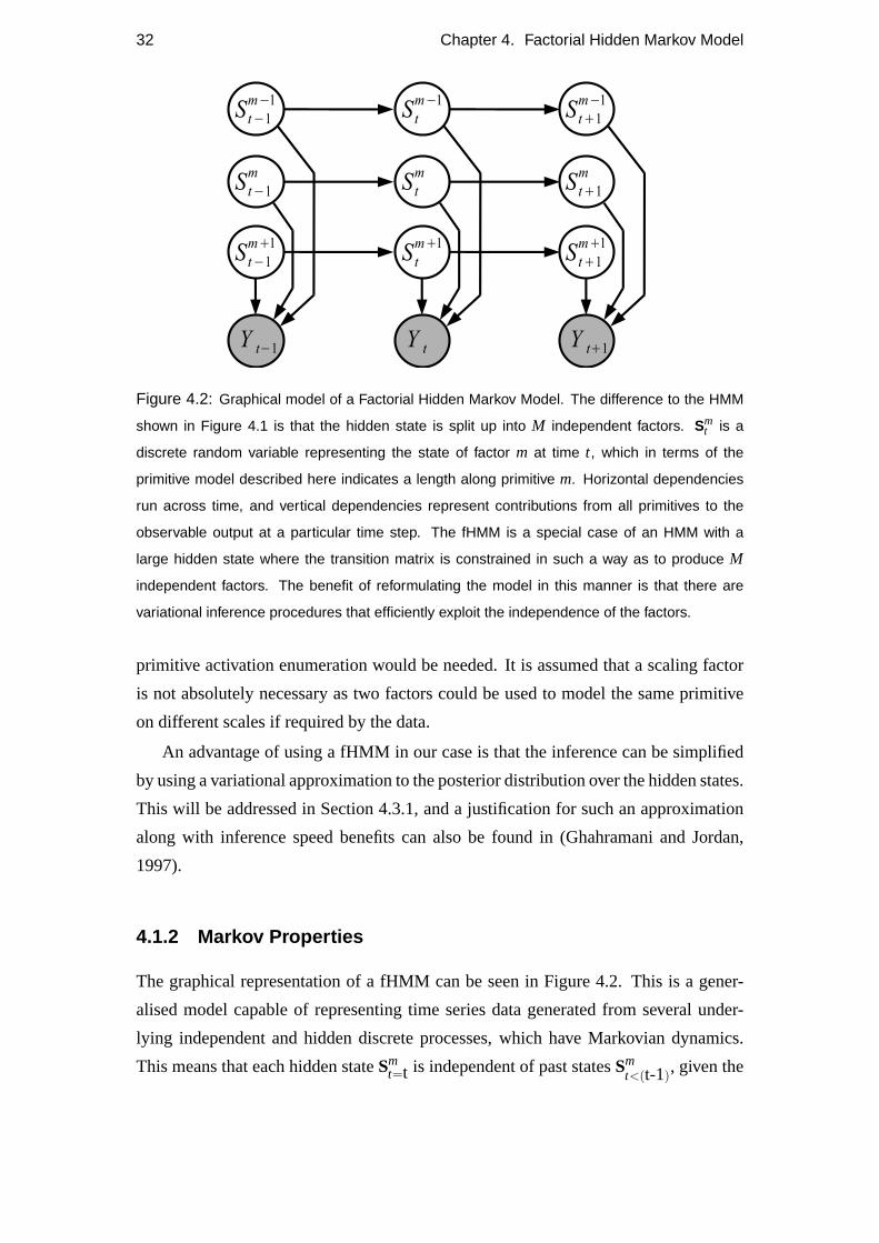
Figure 4.2: Graphical model of a Factorial Hidden Markov Model. The difference to the HMM
shown in Figure 4.1 is that the hidden state is split up into M independent factors. Smt is a
discrete random variable representing the state of factor m at time t, which in terms of the
primitive model described here indicates a length along primitive m. Horizontal dependencies
run across time, and vertical dependencies represent contributions from all primitives to the
observable output at a particular time step. The fHMM is a special case of an HMM with a
large hidden state where the transition matrix is constrained in such a way as to produce M
independent factors. The benefit of reformulating the model in this manner is that there are
variational inference procedures that efficiently exploit the independence of the factors.
primitive activation enumeration would be needed. It is assumed that a scaling factor
is not absolutely necessary as two factors could be used to model the same primitive
on different scales if required by the data.
An advantage of using a fHMM in our case is that the inference can be simplified
by using a variational approximation to the posterior distribution over the hidden states.
This will be addressed in Section 4.3.1, and a justification for such an approximation
along with inference speed benefits can also be found in (Ghahramani and Jordan,
1997).
4.1.2 Markov Properties
The graphical representation of a fHMM can be seen in Figure 4.2. This is a gener-
alised model capable of representing time series data generated from several under-
lying independent and hidden discrete processes, which have Markovian dynamics.
This means that each hidden stateSmt=t is independent of past statesSm
t<(t-1), given the
4.2. Model Definition 33
immediately preceding stateSmt=(t-1). Formally,
P({Sm}) = P(Sm1 )
T
∏t=2
P(Smt |Sm
t−1) . (4.1)
The factors are also independent, meaning that
P({S}) = ∏m
P({Sm}) . (4.2)
In the Piano Model, it is assumed that the pen output is made up of several in-
dependent processes, or primitives. In a fHMM representation of the Piano Model
therefore, the hidden states represent the states of the primitives, with each factor rep-
resenting one primitive. More specifically, the hidden state of factorSmt represents a
length along primitivem, at timet, therefore the set of hidden factors determine the
temporal activity of the primitives. The observable states represent the pen tip data.
4.2 Model Definition
The graphical model for a Factorial Hidden Markov Model can be seen in Figure 4.2.
Here it will be described how the model operates, and how it models the data. Figure
4.3 shows a sample of the data being modelled, both in ‘pen space’ and velocity space.
The velocity data is defined therefore as the observable data. The observable data is the
first differential of pen position and pen tip pressure, and in our case is 3 dimensional,
although I shall refer toD dimensions of the observable data for ease of generalisation.
In Figure 4.4, we can see there is a large degree of variation in the datasets. We will
assume that this variance comes both from noise in the timing of the primitives, and
from the output of the model. We assume that the noise on the output of the model
is Gaussian for modelling convenience.Yt is the random variable representing the
observable output, so if using theD = 3 dimensional data, as described in Section 5.1,
the pen tip velocityYt is defined as
Yt = (x, y, z)T (4.3)
Yt ∼N (µµµt ,C) , (4.4)
whereN denotes a Gaussian distribution.C is a D×D parameter matrix of output
covariance, and
µµµt =M
∑m=1
WmSm
t. (4.5)
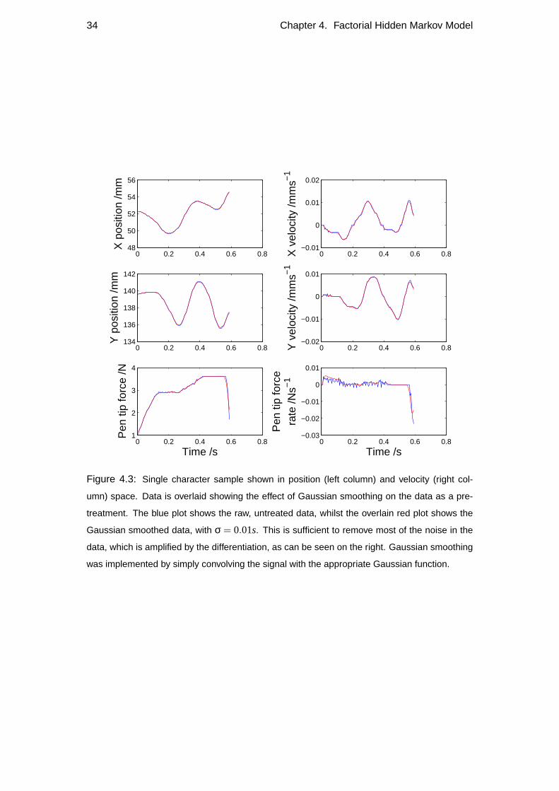
34 Chapter 4. Factorial Hidden Markov Model
0 0.2 0.4 0.6 0.848
50
52
54
56
X p
ositi
on /m
m
0 0.2 0.4 0.6 0.8−0.01
0
0.01
0.02
X v
eloc
ity /m
ms−
1
0 0.2 0.4 0.6 0.8134
136
138
140
142
Y p
ositi
on /m
m
0 0.2 0.4 0.6 0.8−0.02
−0.01
0
0.01
Y v
eloc
ity /m
ms−
1
0 0.2 0.4 0.6 0.81
2
3
4
Time /s
Pen
tip
forc
e /N
0 0.2 0.4 0.6 0.8−0.03
−0.02
−0.01
0
0.01
Time /s
Pen
tip
forc
era
te /N
s−1
Figure 4.3: Single character sample shown in position (left column) and velocity (right col-
umn) space. Data is overlaid showing the effect of Gaussian smoothing on the data as a pre-
treatment. The blue plot shows the raw, untreated data, whilst the overlain red plot shows the
Gaussian smoothed data, with σ = 0.01s. This is sufficient to remove most of the noise in the
data, which is amplified by the differentiation, as can be seen on the right. Gaussian smoothing
was implemented by simply convolving the signal with the appropriate Gaussian function.
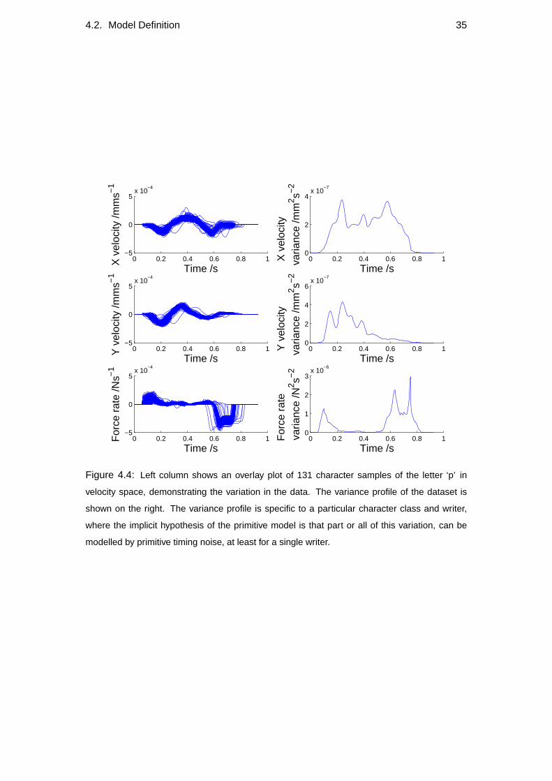
4.2. Model Definition 35
0 0.2 0.4 0.6 0.8 1−5
0
5x 10
−4
Time /s
X v
eloc
ity /m
ms−
1
0 0.2 0.4 0.6 0.8 1−5
0
5x 10
−4
Time /s
Y v
eloc
ity /m
ms−
1
0 0.2 0.4 0.6 0.8 1−5
0
5x 10
−4
Time /s
For
ce r
ate
/Ns−
1
0 0.2 0.4 0.6 0.8 10
2
4x 10
−7
Time /sX
vel
ocity
varia
nce
/mm
2 s−2
0 0.2 0.4 0.6 0.8 10
2
4
6x 10
−7
Time /s
Y v
eloc
ity
va
rianc
e /m
m2 s−
2
0 0.2 0.4 0.6 0.8 10
1
2
3x 10
−6
Time /s
For
ce r
ate
va
rianc
e /N
2 s−2
Figure 4.4: Left column shows an overlay plot of 131 character samples of the letter ‘p’ in
velocity space, demonstrating the variation in the data. The variance profile of the dataset is
shown on the right. The variance profile is specific to a particular character class and writer,
where the implicit hypothesis of the primitive model is that part or all of this variation, can be
modelled by primitive timing noise, at least for a single writer.
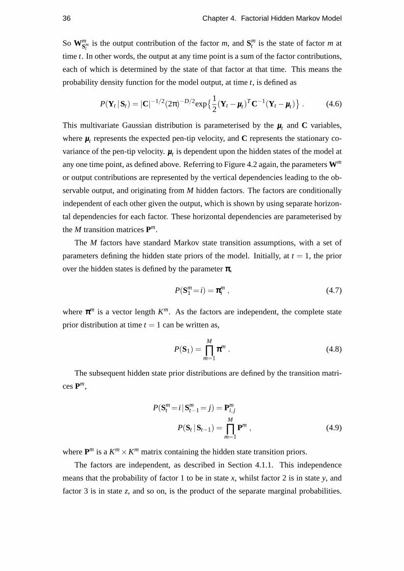
36 Chapter 4. Factorial Hidden Markov Model
So WmSm
tis the output contribution of the factorm, andSm
t is the state of factorm at
time t. In other words, the output at any time point is a sum of the factor contributions,
each of which is determined by the state of that factor at that time. This means the
probability density function for the model output, at timet, is defined as
P(Yt |St) = |C|−1/2(2π)−D/2exp{1
2(Yt−µµµt)
TC−1(Yt−µµµt)}
. (4.6)
This multivariate Gaussian distribution is parameterised by theµµµt and C variables,
whereµµµt represents the expected pen-tip velocity, andC represents the stationary co-
variance of the pen-tip velocity.µµµt is dependent upon the hidden states of the model at
any one time point, as defined above. Referring to Figure 4.2 again, the parametersWm
or output contributions are represented by the vertical dependencies leading to the ob-
servable output, and originating fromM hidden factors. The factors are conditionally
independent of each other given the output, which is shown by using separate horizon-
tal dependencies for each factor. These horizontal dependencies are parameterised by
theM transition matricesPm.
The M factors have standard Markov state transition assumptions, with a set of
parameters defining the hidden state priors of the model. Initially, att = 1, the prior
over the hidden states is defined by the parameterπππ,
P(Sm1 = i) = πππm
i , (4.7)
whereπππm is a vector lengthKm. As the factors are independent, the complete state
prior distribution at timet = 1 can be written as,
P(S1) =M
∏m=1
πππm . (4.8)
The subsequent hidden state prior distributions are defined by the transition matri-
cesPm,
P(Smt = i |Sm
t−1= j) = Pmi, j
P(St |St−1) =M
∏m=1
Pm , (4.9)
wherePm is aKm×Km matrix containing the hidden state transition priors.
The factors are independent, as described in Section 4.1.1. This independence
means that the probability of factor 1 to be in statex, whilst factor 2 is in statey, and
factor 3 is in statez, and so on, is the product of the separate marginal probabilities.
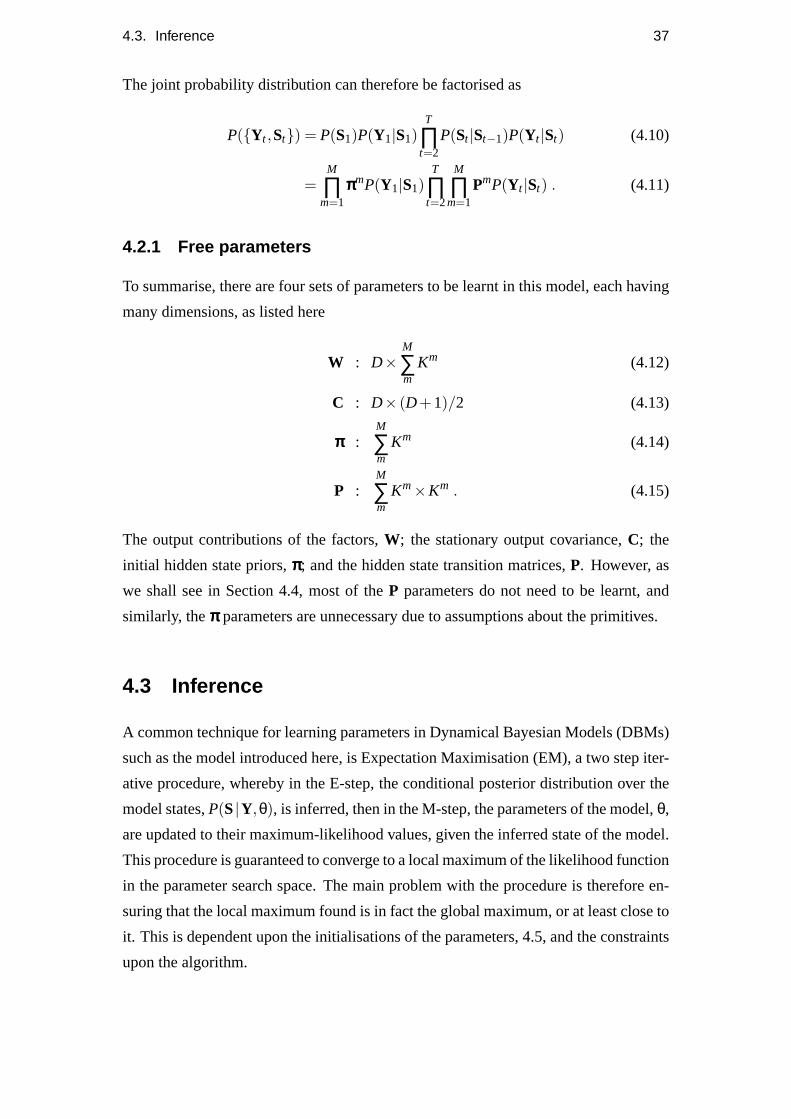
4.3. Inference 37
The joint probability distribution can therefore be factorised as
P({Yt ,St}) = P(S1)P(Y1|S1)T
∏t=2
P(St |St−1)P(Yt |St) (4.10)
=M
∏m=1
πππmP(Y1|S1)T
∏t=2
M
∏m=1
PmP(Yt |St) . (4.11)
4.2.1 Free parameters
To summarise, there are four sets of parameters to be learnt in this model, each having
many dimensions, as listed here
W : D×M
∑m
Km (4.12)
C : D× (D+1)/2 (4.13)
πππ :M
∑m
Km (4.14)
P :M
∑m
Km×Km . (4.15)
The output contributions of the factors,W; the stationary output covariance,C; the
initial hidden state priors,πππ; and the hidden state transition matrices,P. However, as
we shall see in Section 4.4, most of theP parameters do not need to be learnt, and
similarly, theπππ parameters are unnecessary due to assumptions about the primitives.
4.3 Inference
A common technique for learning parameters in Dynamical Bayesian Models (DBMs)
such as the model introduced here, is Expectation Maximisation (EM), a two step iter-
ative procedure, whereby in the E-step, the conditional posterior distribution over the
model states,P(S|Y,θ), is inferred, then in the M-step, the parameters of the model,θ,
are updated to their maximum-likelihood values, given the inferred state of the model.
This procedure is guaranteed to converge to a local maximum of the likelihood function
in the parameter search space. The main problem with the procedure is therefore en-
suring that the local maximum found is in fact the global maximum, or at least close to
it. This is dependent upon the initialisations of the parameters, 4.5, and the constraints
upon the algorithm.
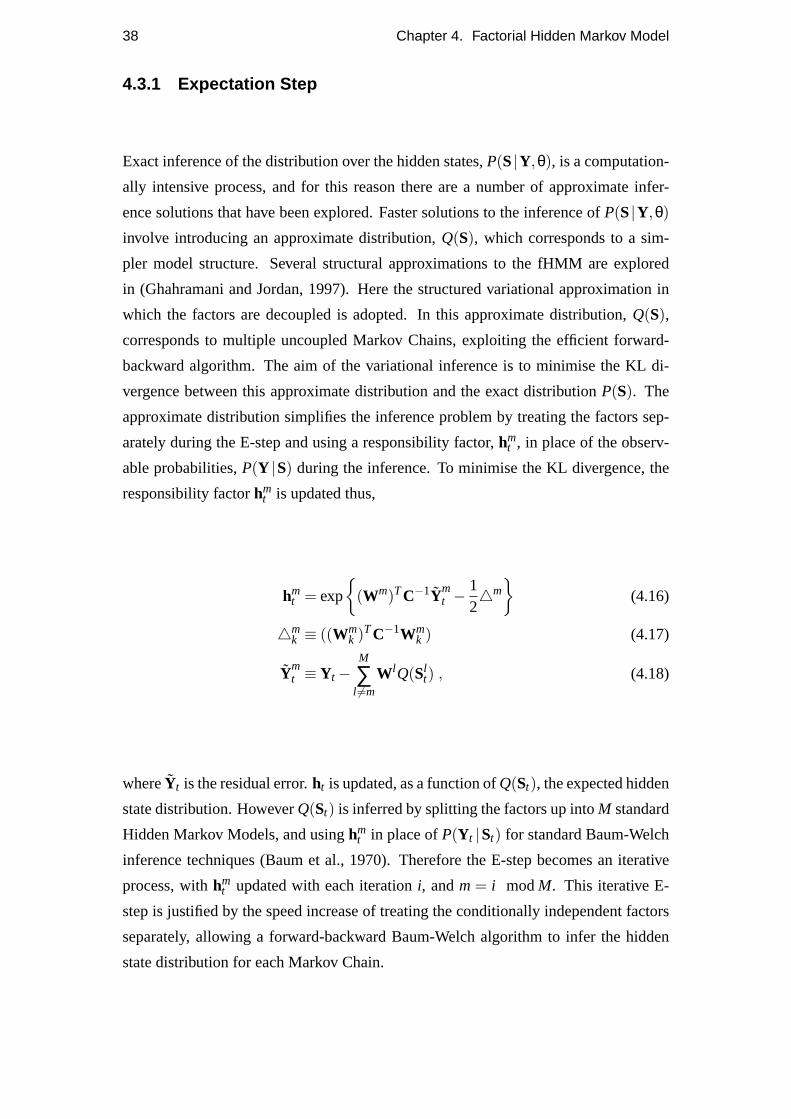
38 Chapter 4. Factorial Hidden Markov Model
4.3.1 Expectation Step
Exact inference of the distribution over the hidden states,P(S|Y,θ), is a computation-
ally intensive process, and for this reason there are a number of approximate infer-
ence solutions that have been explored. Faster solutions to the inference ofP(S|Y,θ)
involve introducing an approximate distribution,Q(S), which corresponds to a sim-
pler model structure. Several structural approximations to the fHMM are explored
in (Ghahramani and Jordan, 1997). Here the structured variational approximation in
which the factors are decoupled is adopted. In this approximate distribution,Q(S),
corresponds to multiple uncoupled Markov Chains, exploiting the efficient forward-
backward algorithm. The aim of the variational inference is to minimise the KL di-
vergence between this approximate distribution and the exact distributionP(S). The
approximate distribution simplifies the inference problem by treating the factors sep-
arately during the E-step and using a responsibility factor,hmt , in place of the observ-
able probabilities,P(Y |S) during the inference. To minimise the KL divergence, the
responsibility factorhmt is updated thus,
hmt = exp
{(Wm)TC−1Ym
t −124m}
(4.16)
4mk ≡ ((Wm
k )TC−1Wmk ) (4.17)
Ymt ≡ Yt−
M
∑l 6=m
W l Q(Slt) , (4.18)
whereYt is the residual error.ht is updated, as a function ofQ(St), the expected hidden
state distribution. HoweverQ(St) is inferred by splitting the factors up intoM standard
Hidden Markov Models, and usinghmt in place ofP(Yt |St) for standard Baum-Welch
inference techniques (Baum et al., 1970). Therefore the E-step becomes an iterative
process, withhmt updated with each iterationi, andm= i modM. This iterative E-
step is justified by the speed increase of treating the conditionally independent factors
separately, allowing a forward-backward Baum-Welch algorithm to infer the hidden
state distribution for each Markov Chain.
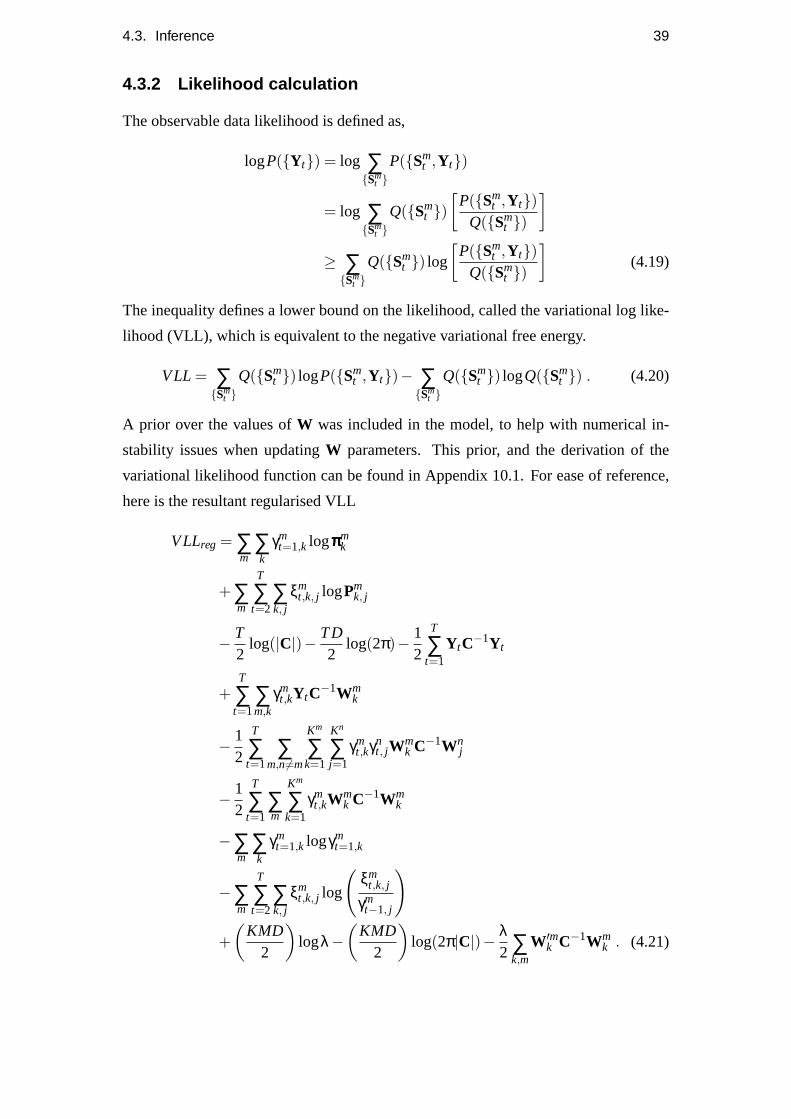
4.3. Inference 39
4.3.2 Likelihood calculation
The observable data likelihood is defined as,
logP({Yt}) = log ∑{Sm
t }P({Sm
t ,Yt})
= log ∑{Sm
t }Q({Sm
t })[
P({Smt ,Yt})
Q({Smt })
]≥ ∑{Sm
t }Q({Sm
t }) log
[P({Sm
t ,Yt})Q({Sm
t })
](4.19)
The inequality defines a lower bound on the likelihood, called the variational log like-
lihood (VLL), which is equivalent to the negative variational free energy.
VLL = ∑{Sm
t }Q({Sm
t }) logP({Smt ,Yt})− ∑
{Smt }
Q({Smt }) logQ({Sm
t }) . (4.20)
A prior over the values ofW was included in the model, to help with numerical in-
stability issues when updatingW parameters. This prior, and the derivation of the
variational likelihood function can be found in Appendix 10.1. For ease of reference,
here is the resultant regularised VLL
VLLreg = ∑m
∑k
γmt=1,k logπππm
k
+∑m
T
∑t=2
∑k, j
ξmt,k, j logPm
k, j
− T2
log(|C|)− TD2
log(2π)− 12
T
∑t=1
YtC−1Yt
+T
∑t=1
∑m,k
γmt,kYtC−1Wm
k
− 12
T
∑t=1
∑m,n6=m
Km
∑k=1
Kn
∑j=1
γmt,kγn
t, jWmk C−1Wn
j
− 12
T
∑t=1
∑m
Km
∑k=1
γmt,kW
mk C−1Wm
k
−∑m
∑k
γmt=1,k logγm
t=1,k
−∑m
T
∑t=2
∑k, j
ξmt,k, j log
(ξm
t,k, j
γmt−1, j
)
+(
KMD2
)logλ−
(KMD
2
)log(2π|C|)− λ
2 ∑k,m
W′mk C−1Wmk . (4.21)
40 Chapter 4. Factorial Hidden Markov Model
To conform to the standard notation conventions,Q(Smt = k) is written asγm
t,k, which is
the probability that the hidden state of factorm takes the valuek at timet. Likewise,
Q(Smt = k,Sm
t−1 = j) = ξmt,k, j , which is the joint probability that the hidden state of
factorm takes the valuek at timet andand takes the value ofj at timet−1. Kx is the
number of hidden states in primitivex, andK = ∑xKx, which is the number of hidden
states in the whole model.
4.3.3 Maximisation Step
The M-step updates the parameters to their maximum likelihood values.
W← (T
∑t=1
YtQ(St)′)(T
∑t=1
Q(St)Q(St)′+λI)† (4.22)
πππ(m)←Q(Sm1 ) (4.23)
Pmi, j ←
∑Tt=2Q(Sm
t = i,Smt−1 = j)
∑Tt=2Q(Sm
t−1 = j)(4.24)
C← 1T
T
∑t=1
YtY′t−1T
T
∑t=1
M
∑m=1
WmQ(Smt )Y′t (4.25)
Q(St) is the distribution over the hidden states of the model, or the expected value of
the hidden states at timet. † meanspseudo-inverse. Wm is the contribution of factorm
to the output mean.W is a concatenated matrix of all these means, thus storing all the
primitives. TheW update includes a regularisation factor,λ, as described in Section
4.3.2. Yt is the observable output vector. As all the M-step updates are summations
over time, it is easier to implement this with separate character samples, by gathering
the statistics during the E-step.
4.4 Constraints and modifications
Several constraints and modifications were made to the model. The constraints were
made so that the learnt probabilistic models have the same structure as the Piano
Model, as described in Chapter 3. The constraints do not affect the likelihood from
one EM iteration to the next; however, without the constraints, a higher likelihood
could be obtained.
The modifications to the algorithm are heuristic optimisation techniques to avoid
local maxima in the likelihood function. They are heuristic because calculating the
likelihood for the model takes a lot of computation, and it is not feasible to perform
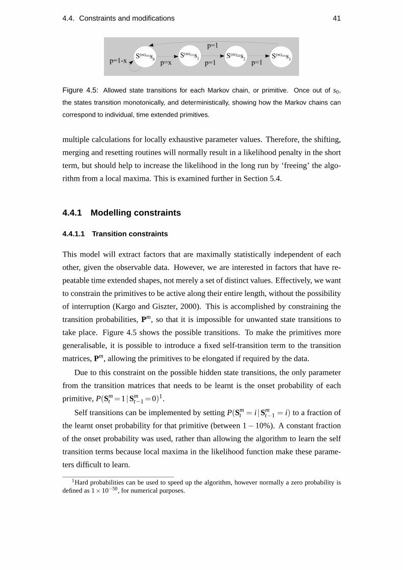
4.4. Constraints and modifications 41
Figure 4.5: Allowed state transitions for each Markov chain, or primitive. Once out of s0,
the states transition monotonically, and deterministically, showing how the Markov chains can
correspond to individual, time extended primitives.
multiple calculations for locally exhaustive parameter values. Therefore, the shifting,
merging and resetting routines will normally result in a likelihood penalty in the short
term, but should help to increase the likelihood in the long run by ‘freeing’ the algo-
rithm from a local maxima. This is examined further in Section 5.4.
4.4.1 Modelling constraints
4.4.1.1 Transition constraints
This model will extract factors that are maximally statistically independent of each
other, given the observable data. However, we are interested in factors that have re-
peatable time extended shapes, not merely a set of distinct values. Effectively, we want
to constrain the primitives to be active along their entire length, without the possibility
of interruption (Kargo and Giszter, 2000). This is accomplished by constraining the
transition probabilities,Pm, so that it is impossible for unwanted state transitions to
take place. Figure 4.5 shows the possible transitions. To make the primitives more
generalisable, it is possible to introduce a fixed self-transition term to the transition
matrices,Pm, allowing the primitives to be elongated if required by the data.
Due to this constraint on the possible hidden state transitions, the only parameter
from the transition matrices that needs to be learnt is the onset probability of each
primitive, P(Smt =1|Sm
t−1=0)1.
Self transitions can be implemented by settingP(Smt = i |Sm
t−1 = i) to a fraction of
the learnt onset probability for that primitive (between 1−10%). A constant fraction
of the onset probability was used, rather than allowing the algorithm to learn the self
transition terms because local maxima in the likelihood function make these parame-
ters difficult to learn.
1Hard probabilities can be used to speed up the algorithm, however normally a zero probability isdefined as 1×10−50, for numerical purposes.
42 Chapter 4. Factorial Hidden Markov Model
4.4.1.2 Zero State Assumptions
The model does not provide automatically for anoff state for the primitives, as each
state has an associated output contribution. We assume that the primitives are time-
extended, but not continuously active throughout the entire data sequence, (i.e. charac-
ter) and so we constrain the primitives to have a zero state, with zero output contribu-
tions in all data dimensions. This is easily done by settingWm1 = 0 in the M-step, and
not learning these parameters. It is expected that the primitives will be sparsely used,
and so this rest state will be the norm, with a correspondingly large self-transition term
in theWm matrices, learnt during EM.
4.4.2 Heuristic optimisations
4.4.2.1 Shifting
There are many local maxima in the parameter search space, as demonstrated when
running the algorithm on an artificially generated dataset, containing planted motifs,
see Figure 4.6. The primitives would ‘latch on’ to certain parts of the motifs, and if
thestart of a learnt primitive becomes a good representation for theendof a planted
motif in the data, the algorithm would find it difficult to learn the rest of the motif. This
problem was addressed by introducing a shifting/extension heuristic, which examines
the start and the end of the primitives. The reasoning behind this decision was that if
a motif is being partially represented by a factor, then the shifting algorithm would be
able to extend the factor to include the rest of the motif, whereas if a motif is entirely
represented by a factor, then by averaging over many character samples, the learnt
values outside of the motif should be equal to zero, therefore the primitive would not
be extended. An example can be seen in Figure 4.7, where the dotted lines represent
the specific cut offs for the primitive being examined, and are 3 dimensional.
To determine whether a particular primitive should be shifted, the start and end
sections of the primitives are examined. If the mean absolute value of any dimension
of the examined section is above a constant ‘body definition’ fraction of the mean ab-
solute value of the whole primitive, then the section is assumed to be part of the motif,
and is extended. Otherwise, if the square of all dimensions are below a ‘zero defini-
tion’ fraction of the primitive, then the section is assumed to be outside the motif being
captured by the primitive, and the section is therefore ‘pruned’. It should be noted
that the length of the primitives is not fixed, and is defined therefore by this shifting
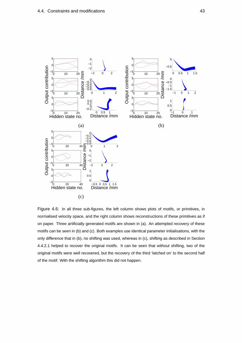
4.4. Constraints and modifications 43
0 10 20−5
0
5
−2 0 2
−2
−1
0
0 10 20−5
0
5
Out
put c
ontr
ibut
ion
0 1 2−0.8−0.6−0.4−0.2
0D
ista
nce
/mm
0 10 20−5
0
5
Hidden state no.0 0.5 1
−0.20
0.20.4
Distance /mm
0 10 20−5
0
5
0 0.5 1 1.5
−0.5
0
0 10 20−5
0
5
Out
put c
ontr
ibut
ion
−1 0 1 2−1.5
−1−0.5
0
Dis
tanc
e /m
m
0 10 20−5
0
5
Hidden state no.−1 0 1
0
0.5
1
Distance /mm
(a) (b)
0 20 40−5
0
5
0 1 2−0.8−0.6−0.4−0.2
0
0 20 40−5
0
5
Out
put c
ontr
ibut
ion
−2 0 2
−2
−1
0
Dis
tanc
e /m
m
0 20 40−5
0
5
Hidden state no.−0.5 0 0.5 1 1.5
0
0.5
1
Distance /mm
(c)
Figure 4.6: In all three sub-figures, the left column shows plots of motifs, or primitives, in
normalised velocity space, and the right column shows reconstructions of these primitives as if
on paper. Three artificially generated motifs are shown in (a). An attempted recovery of these
motifs can be seen in (b) and (c). Both examples use identical parameter initialisations, with the
only difference that in (b), no shifting was used, whereas in (c), shifting as described in Section
4.4.2.1 helped to recover the original motifs. It can be seen that without shifting, two of the
original motifs were well recovered, but the recovery of the third ‘latched on’ to the second half
of the motif. With the shifting algorithm this did not happen.
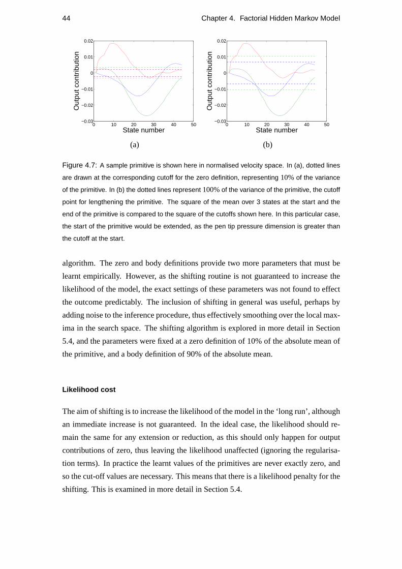
44 Chapter 4. Factorial Hidden Markov Model
0 10 20 30 40 50−0.03
−0.02
−0.01
0
0.01
0.02
State number
Out
put c
ontr
ibut
ion
0 10 20 30 40 50−0.03
−0.02
−0.01
0
0.01
0.02
State number
Out
put c
ontr
ibut
ion
(a) (b)
Figure 4.7: A sample primitive is shown here in normalised velocity space. In (a), dotted lines
are drawn at the corresponding cutoff for the zero definition, representing 10%of the variance
of the primitive. In (b) the dotted lines represent 100%of the variance of the primitive, the cutoff
point for lengthening the primitive. The square of the mean over 3 states at the start and the
end of the primitive is compared to the square of the cutoffs shown here. In this particular case,
the start of the primitive would be extended, as the pen tip pressure dimension is greater than
the cutoff at the start.
algorithm. The zero and body definitions provide two more parameters that must be
learnt empirically. However, as the shifting routine is not guaranteed to increase the
likelihood of the model, the exact settings of these parameters was not found to effect
the outcome predictably. The inclusion of shifting in general was useful, perhaps by
adding noise to the inference procedure, thus effectively smoothing over the local max-
ima in the search space. The shifting algorithm is explored in more detail in Section
5.4, and the parameters were fixed at a zero definition of 10% of the absolute mean of
the primitive, and a body definition of 90% of the absolute mean.
Likelihood cost
The aim of shifting is to increase the likelihood of the model in the ‘long run’, although
an immediate increase is not guaranteed. In the ideal case, the likelihood should re-
main the same for any extension or reduction, as this should only happen for output
contributions of zero, thus leaving the likelihood unaffected (ignoring the regularisa-
tion terms). In practice the learnt values of the primitives are never exactly zero, and
so the cut-off values are necessary. This means that there is a likelihood penalty for the
shifting. This is examined in more detail in Section 5.4.

4.4. Constraints and modifications 45
Pseudo code
SHIFT
Calculate cutoff points for shifting:
1 zerodef≡ 10% of mean absolute value of primitive
2 bodydef≡ 90% of mean absolute value of primitive
3 testsections= mean absolute value over 3 samples at start and end of primitives
4 if any dimension of atestsection> bodydef
5 then extend the primitive
6 else ifall dimensions of thetestsection< zerodef
7 then shorten the primitive
4.4.2.2 Merging
Sections of primitives can sometimes start to model similar sections of the data. If
two primitives become close to identical, then they should be merged, to help with
generalisation. This merging problem was resolved by examining the mean squared
difference between primitives, which, if smaller than a defined fraction of the variance
of the primitives (in all dimensions), then the primitives are flagged as the same, and
so merged by setting one to the average of both, and resetting the other. The other
variables, such asQ(Smt ) were altered accordingly, preserving the onsets of the two
original primitives in the new merged primitive, and resetting the onsets of the new
reset primitive. Therefore the new merged primitive assumes the average shape of the
two original primitives, and all the onset positions of both original primitives.
Figure 4.8 shows an example of a primitive and the ranges of potential primitives
that would be merged using this algorithm, with a cutoff placed at 50% of the primitive
variance. The examples given are the extremes, with the entire length of the primitive
on the borderline of the merging cutoff. In practice merging does not occur as ex-
cessively as is perhaps suggested by these plots, as the EM algorithm will try to find
primitives that best explain the data, therefore unless the data only contains a single
motif, with very little noise, the primitives learnt will not normally be identical to each
other.
It should be noted that for primitives of different lengths, the comparison is done
by sliding the shorter of the two primitives along the length of the longer one, giving
the average mean squared difference at several offsets. If this mean squared difference
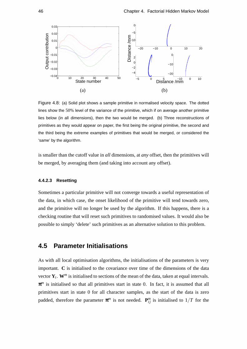
46 Chapter 4. Factorial Hidden Markov Model
0 10 20 30 40 50−0.04
−0.03
−0.02
−0.01
0
0.01
0.02
0.03
State number
Out
put c
ontr
ibut
ion
−20 −10 0 10 20
−10
−5
0
−5 0 5
−4
−2
0
2
Distance /mm
Dis
tanc
e /m
m
−10 0 10
−20
−10
0
(a) (b)
Figure 4.8: (a) Solid plot shows a sample primitive in normalised velocity space. The dotted
lines show the 50% level of the variance of the primitive, which if on average another primitive
lies below (in all dimensions), then the two would be merged. (b) Three reconstructions of
primitives as they would appear on paper, the first being the original primitive, the second and
the third being the extreme examples of primitives that would be merged, or considered the
‘same’ by the algorithm.
is smaller than the cutoff value inall dimensions, atanyoffset, then the primitives will
be merged, by averaging them (and taking into account any offset).
4.4.2.3 Resetting
Sometimes a particular primitive will not converge towards a useful representation of
the data, in which case, the onset likelihood of the primitive will tend towards zero,
and the primitive will no longer be used by the algorithm. If this happens, there is a
checking routine that will reset such primitives to randomised values. It would also be
possible to simply ‘delete’ such primitives as an alternative solution to this problem.
4.5 Parameter Initialisations
As with all local optimisation algorithms, the initialisations of the parameters is very
important. C is initialised to the covariance over time of the dimensions of the data
vectorYt . Wm is initialised to sections of the mean of the data, taken at equal intervals.
πππm is initialised so that all primitives start in state 0. In fact, it is assumed that all
primitives start in state 0 for all character samples, as the start of the data is zero
padded, therefore the parameterπππm is not needed.Pmi j is initialised to 1/T for the

4.5. Parameter Initialisations 47
onset transition, and the deterministic state transitions as described above, for other
transitions.
The initialisations of the primitive shapes are contained in the parameter matrix
Wm, and are extremely important, and have an effect upon the resultant primitives.
It is suggested in Chapter 9 that these parameters be initialised by some fast greedy
algorithm to help with finding a repeatable solution to this local optimisation problem.

Chapter 5
Factorial Hidden Markov Model
Results
In Chapter 4 we discuss in detail a model for representing handwriting data using
time-extended primitives. This Factorial Hidden Markov Model (fHMM) represents
pen movement primitives in the the form of parameters, and the states of these prim-
itives are represented in the hidden states of the model. The state of the model can
be approximated with a set of primitive timings giving rise to a particular character
reproduction, and as such does not generalise across character samples, as this timing,
or onset of the primitives is represented in the posterior over the hidden states of the
model. However, the shapes of the primitives themselves, and how they model the
variance of the data is interesting, and will be examined in this chapter. The repeata-
bility of the inference, and therefore reliability of primitive extraction will be assessed,
and the generalisation of the model for test data, based on similar, or novel characters
will be examined.
Finally the generative behaviour of the model will be demonstrated, highlighting
the need for a further level of modelling that allows the primitives to generalise across
different character samples.
5.1 Data
The raw data comes from an INTUOS 3 WACOM digitisation tablethttp://www.
wacom.com/productinfo/9x12.cfm, providing 200Hz pen tip position data capture.
The tablet uses an electromagnetic field to detect the position and orientation of the
penhttp://www.wacom-components.com/english/technology/emr.html. The
49
50 Chapter 5. Factorial Hidden Markov Model Results
pressure of the writing is detected using a pressure sensor in the tip of the pen, which
modulates the field and is read by the tablet. The pen tip pressure (technically force,
of course) information is digitised to 1,024 discrete levels, for a desired range of 30−400g, or 0.29−3.92N giving a resolution of 3.53mN. When the pen is not in contact
with the tablet, position information is still detected, up to a height of 6mm. The
resolution of the pen position is given as 5,080 lines per inch, however, the accuracy
is given as±0.25mm. Assuming the latter is the case, this gives the useable resolution
of the pen position as 0.5mm, or 51 lines per inch. If, however, the accuracy derives
from some locally smooth offset, due to non-linearities in the electromagnetic field,
as is likely to be the case, then the useable resolution for a small area is much better.
Samples of the raw data can be seen in Figure 5.1, and of the same, differentiated data
in Figure 5.2. The signal to noise ratio of the pen tilt and pen orientation dimensions
was too low for useful information to be gained, and it was found that including this
data diminished the performance of the model, therefore only the first three dimensions
of the data were used. For ease of generalisation however, I will refer toD dimensions
of the data.
We wish the primitives to be as generally applicable as possible, and not limited
intentionally to certain parts of characters. We also need to remove any constant offset
in the data (arising from drift in position of character drawing). This could be ac-
complished by subtracting the mean for each character sample, but it does not solve
the problem within a character. To model the data using a fixed function model, we
want the data to be normalised, and roughly zero centred, therefore it was decided to
model the velocity, or first differential of the data. Normalisation of the dataset helps
the model to be applicable over multiple scales. The differentiated (velocity) data may
well be a better representation of the internal biological code for the muscle activa-
tions, as these are very unlikely to be in absolute coordinates, and would be expected
to reflect either velocity or acceleration of the system. Other possible representations
include affine geometrical transformations such as those proposed by (T. Flash, 2007).
Before differentiating the data, it was smoothed using a Gaussian filter to reduce the
amplification of noise due to numerical differentiation. There are more sophisticated
smoothing methods such as those used in (Ramsay, 2000). Gaussian smoothing was
chosen for its simplicity and repeatable predictability of behaviour. The difference be-
tween the raw and smoothed data can be seen in Figure 5.3. In this figure, it can be
seen that without smoothing, the first differential of the data is quite noisy, especially
the pen tip pressure data.
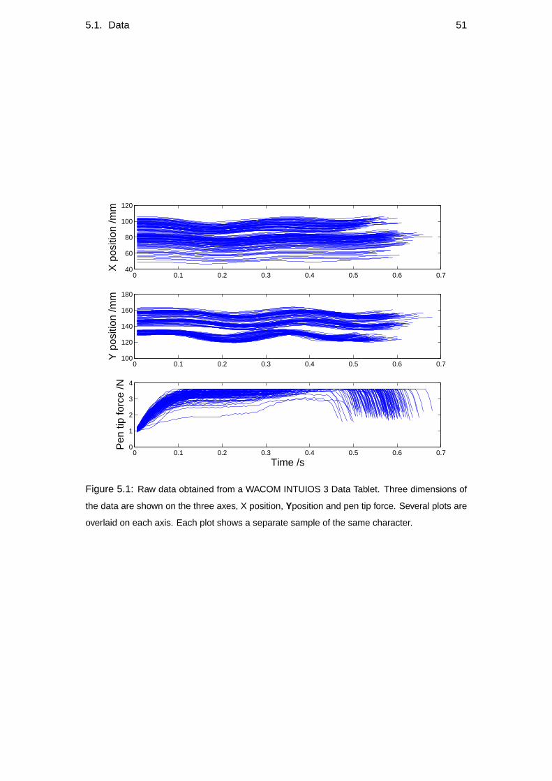
5.1. Data 51
0 0.1 0.2 0.3 0.4 0.5 0.6 0.740
60
80
100
120
X p
ositi
on /m
m
0 0.1 0.2 0.3 0.4 0.5 0.6 0.7100
120
140
160
180
Y p
ositi
on /m
m
0 0.1 0.2 0.3 0.4 0.5 0.6 0.70
1
2
3
4
Time /s
Pen
tip
forc
e /N
Figure 5.1: Raw data obtained from a WACOM INTUIOS 3 Data Tablet. Three dimensions of
the data are shown on the three axes, X position, Yposition and pen tip force. Several plots are
overlaid on each axis. Each plot shows a separate sample of the same character.
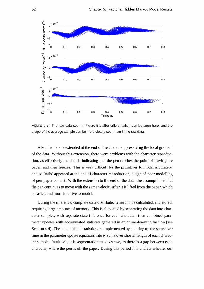
52 Chapter 5. Factorial Hidden Markov Model Results
0 0.1 0.2 0.3 0.4 0.5 0.6 0.7 0.8−4
−2
0
2x 10
−4
X v
eloc
ity /m
ms−
1
0 0.1 0.2 0.3 0.4 0.5 0.6 0.7 0.8−2
0
2x 10
−4
Y v
eloc
ity /m
ms−
1
0 0.1 0.2 0.3 0.4 0.5 0.6 0.7 0.8−10
−5
0
5x 10
−4
Time /s
For
ce r
ate
/Ns−
1
Figure 5.2: The raw data seen in Figure 5.1 after differentiation can be seen here, and the
shape of the average sample can be more clearly seen than in the raw data.
Also, the data is extended at the end of the character, preserving the local gradient
of the data. Without this extension, there were problems with the character reproduc-
tion, as effectively the data is indicating that the pen reaches the point of leaving the
paper, and then freezes. This is very difficult for the primitives to model accurately,
and so ‘tails’ appeared at the end of character reproduction, a sign of poor modelling
of pen-paper contact. With the extension to the end of the data, the assumption is that
the pen continues to move with the same velocity after it is lifted from the paper, which
is easier, and more intuitive to model.
During the inference, complete state distributions need to be calculated, and stored,
requiring large amounts of memory. This is alleviated by separating the data into char-
acter samples, with separate state inference for each character, then combined para-
meter updates with accumulated statistics gathered in an online-learning fashion (see
Section 4.4). The accumulated statistics are implemented by splitting up the sums over
time in the parameter update equations intoN sums over shorter length of each charac-
ter sample. Intuitively this segmentation makes sense, as there is a gap between each
character, where the pen is off the paper. During this period it is unclear whether our
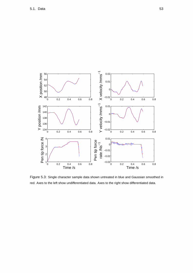
5.1. Data 53
0 0.2 0.4 0.6 0.848
50
52
54
56
X p
ositi
on /m
m
0 0.2 0.4 0.6 0.8−0.01
0
0.01
0.02
X v
eloc
ity /m
ms−
1
0 0.2 0.4 0.6 0.8134
136
138
140
142
Y p
ositi
on /m
m
0 0.2 0.4 0.6 0.8−0.02
−0.01
0
0.01
Y v
eloc
ity /m
ms−
1
0 0.2 0.4 0.6 0.81
2
3
4
Time /s
Pen
tip
forc
e /N
0 0.2 0.4 0.6 0.8−0.03
−0.02
−0.01
0
0.01
Time /s
Pen
tip
forc
era
te /N
s−1
Figure 5.3: Single character sample data shown untreated in blue and Gaussian smoothed in
red. Axes to the left show undifferentiated data. Axes to the right show differentiated data.
54 Chapter 5. Factorial Hidden Markov Model Results
model would be sufficient for modelling the primitives involved in the pen tip motion;
also the dimension of the data would be reduced, as the pen tip pressure would not give
any information. Furthermore, any pen off-paper motion would be a function of the
previous and subsequent characters to be drawn, and other higher level, unmodelled ef-
fects (such as breaks from data entry). The cut-off point forpen upregions was defined
as 250, or 0.88N, empirically giving the whole character, whilst removingpen bounce
noise. Currently, there is no provision for characters that require two separate strokes,
where the pen must leave the paper within the drawing of the character. This drawback
could be removed by including some random variable indicating when a character is
being drawn, which would couple the two parts of the character together. This setup
would be greatly improved with visual feedback, as we naıvely group pen strokes into
single characters based upon spacial coherence; i.e. the dots need to be above or at
least near thei’s, and the dashes need to cross thet’s.
In a given dataset,n enumerates the character samples, of varying length, so for
each character sample,Yn, is a D× Tn matrix of observable variables, whereD is
the dimension of the data (3 in this application) andTn is the number of samples in
charactern. For ease of notation whilst describing the model, the sample number will
be subsequently omitted, and the observable data can be thought of as a concatenation
of the separate samples unless stated otherwise. The data is normally time indexed,
makingYt a vector of lengthD.
5.1.1 Datasets Used
Several different datasets were used for training purposes. Here the most commonly
used datasets are described:
Artificially generated dataset Five artificially generated primitives were used to gen-
erate a dummy dataset, using the fHMM as a generative model, with the con-
straints and assumptions used for the learning procedure. Figure 5.4 shows the
primitives used, and some dataset samples as they would appear reproduced on
paper. The length and number of primitives, as well as other parameters, such
as self transition priors, were configurable, allowing testing of various aspects of
the algorithm.
‘p’ dataset A sub-sampled dataset composed of the character‘p’ consisted of 131
character samples. Figure 5.5 shows the variance profile of this dataset.
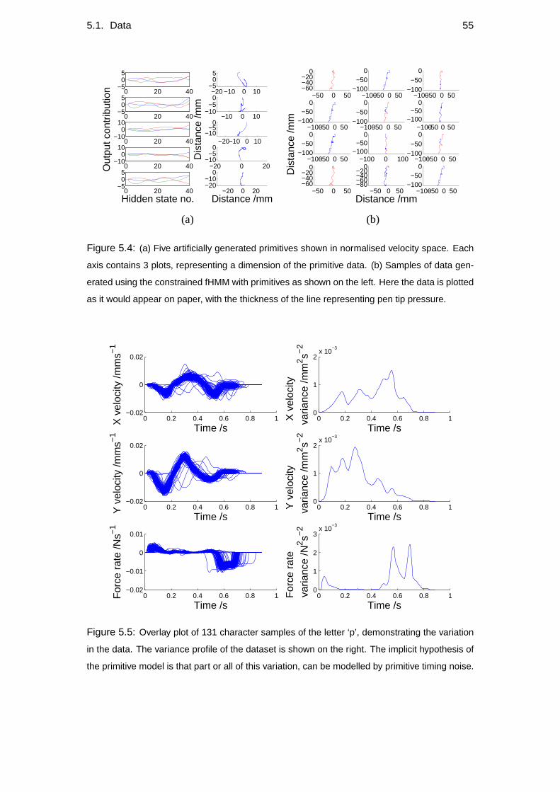
5.1. Data 55
0 20 40−5
05
−20 −10 0 10−5
05
0 20 40−5
05
−10 0 10−10
−50
0 20 40−10
010
Out
put c
ontr
ibut
ion
−20−10 0 10−10
−50
Dis
tanc
e /m
m
0 20 40−10
010
−20 0 20−10
−50
0 20 40−5
05
Hidden state no.−20 0 20
−20−10
0
Distance /mm
−50 0 50−60−40−20
0
−100−50 0 50−100−50
0
−100−50 0 50−100−50
0
−100−50 0 50−100−50
0
−100−50 0 50−100−50
0
−100−50 0 50−100−50
0
−100−50 0 50−100−50
0
Dis
tanc
e /m
m
−100 0 100−100−50
0
−100−50 0 50−100−50
0
−50 0 50−60−40−20
0
−50 0 50−80−60−40−20
0
Distance /mm−100−50 0 50
−100−50
0
(a) (b)
Figure 5.4: (a) Five artificially generated primitives shown in normalised velocity space. Each
axis contains 3 plots, representing a dimension of the primitive data. (b) Samples of data gen-
erated using the constrained fHMM with primitives as shown on the left. Here the data is plotted
as it would appear on paper, with the thickness of the line representing pen tip pressure.
0 0.2 0.4 0.6 0.8 1−0.02
0
0.02
Time /s
X v
eloc
ity /m
ms−
1
0 0.2 0.4 0.6 0.8 1−0.02
0
0.02
Time /s
Y v
eloc
ity /m
ms−
1
0 0.2 0.4 0.6 0.8 1−0.02
−0.01
0
0.01
Time /s
For
ce r
ate
/Ns−
1
0 0.2 0.4 0.6 0.8 10
1
2x 10
−3
Time /s
X v
eloc
ity
va
rianc
e /m
m2 s−
2
0 0.2 0.4 0.6 0.8 10
1
2x 10
−3
Time /s
Y v
eloc
ity
va
rianc
e /m
m2 s−
2
0 0.2 0.4 0.6 0.8 10
1
2
3x 10
−3
Time /s
For
ce r
ate
va
rianc
e /N
2 s−2
Figure 5.5: Overlay plot of 131 character samples of the letter ‘p’, demonstrating the variation
in the data. The variance profile of the dataset is shown on the right. The implicit hypothesis of
the primitive model is that part or all of this variation, can be modelled by primitive timing noise.
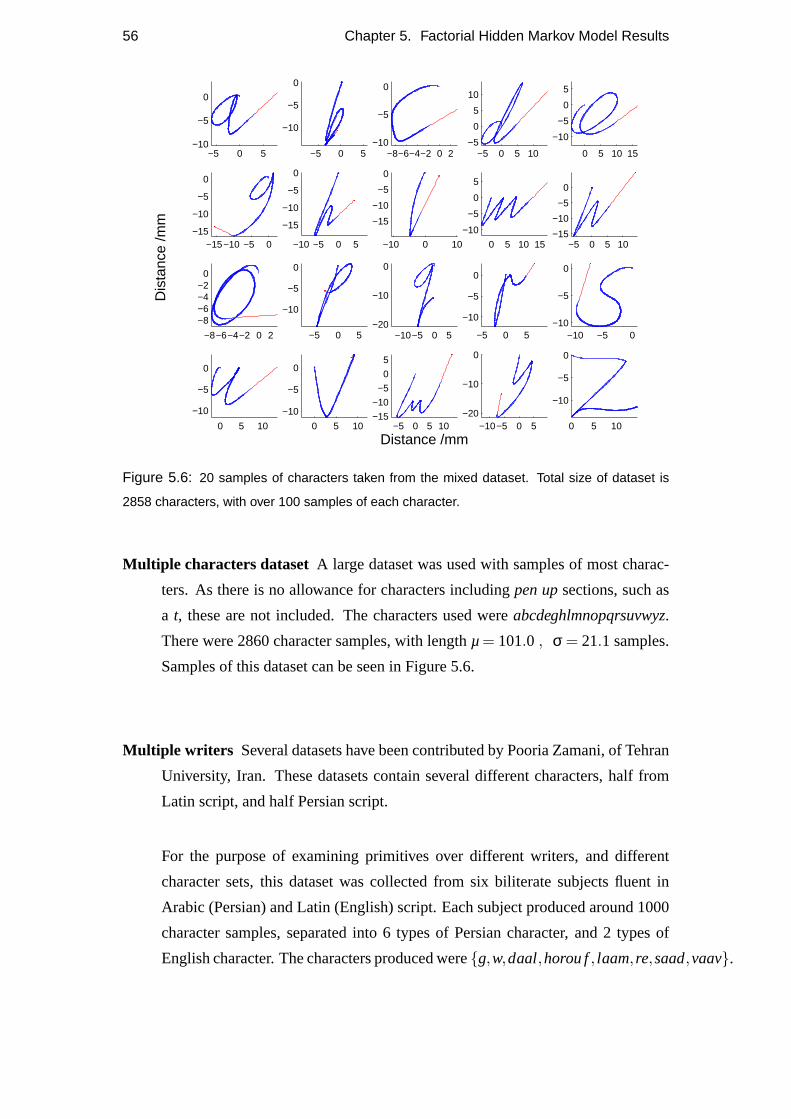
56 Chapter 5. Factorial Hidden Markov Model Results
−5 0 5−10
−5
0
−5 0 5
−10
−5
0
−8−6−4−2 0 2−10
−5
0
−5 0 5 10−5
0
5
10
0 5 10 15
−10
−5
0
5
−15−10 −5 0−15
−10
−5
0
Dis
tanc
e /m
m
−10 −5 0 5
−15
−10
−5
0
−10 0 10
−15
−10
−5
0
0 5 10 15
−10
−5
0
5
−5 0 5 10−15
−10
−5
0
−8−6−4−2 0 2
−8−6−4−2
0
−5 0 5
−10
−5
0
−10−5 0 5−20
−10
0
−5 0 5
−10
−5
0
−10 −5 0−10
−5
0
0 5 10
−10
−5
0
0 5 10
−10
−5
0
−5 0 5 10−15
−10
−5
0
5
Distance /mm−10−5 0 5
−20
−10
0
0 5 10
−10
−5
0
Figure 5.6: 20 samples of characters taken from the mixed dataset. Total size of dataset is
2858 characters, with over 100 samples of each character.
Multiple characters dataset A large dataset was used with samples of most charac-
ters. As there is no allowance for characters includingpen upsections, such as
a t, these are not included. The characters used wereabcdeghlmnopqrsuvwyz.
There were 2860 character samples, with lengthµ= 101.0 , σ = 21.1 samples.
Samples of this dataset can be seen in Figure 5.6.
Multiple writers Several datasets have been contributed by Pooria Zamani, of Tehran
University, Iran. These datasets contain several different characters, half from
Latin script, and half Persian script.
For the purpose of examining primitives over different writers, and different
character sets, this dataset was collected from six biliterate subjects fluent in
Arabic (Persian) and Latin (English) script. Each subject produced around 1000
character samples, separated into 6 types of Persian character, and 2 types of
English character. The characters produced were{g,w,daal,horou f, laam, re,saad,vaav}.
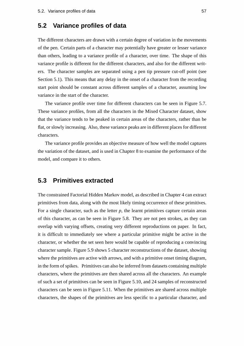
5.2. Variance profiles of data 57
5.2 Variance profiles of data
The different characters are drawn with a certain degree of variation in the movements
of the pen. Certain parts of a character may potentially have greater or lesser variance
than others, leading to a variance profile of a character, over time. The shape of this
variance profile is different for the different characters, and also for the different writ-
ers. The character samples are separated using a pen tip pressure cut-off point (see
Section 5.1). This means that any delay in the onset of a character from the recording
start point should be constant across different samples of a character, assuming low
variance in the start of the character.
The variance profile over time for different characters can be seen in Figure 5.7.
These variance profiles, from all the characters in the Mixed Character dataset, show
that the variance tends to be peaked in certain areas of the characters, rather than be
flat, or slowly increasing. Also, these variance peaks are in different places for different
characters.
The variance profile provides an objective measure of how well the model captures
the variation of the dataset, and is used in Chapter 8 to examine the performance of the
model, and compare it to others.
5.3 Primitives extracted
The constrained Factorial Hidden Markov model, as described in Chapter 4 can extract
primitives from data, along with the most likely timing occurrence of these primitives.
For a single character, such as the letterp, the learnt primitives capture certain areas
of this character, as can be seen in Figure 5.8. They are not pen strokes, as they can
overlap with varying offsets, creating very different reproductions on paper. In fact,
it is difficult to immediately see where a particular primitive might be active in the
character, or whether the set seen here would be capable of reproducing a convincing
character sample. Figure 5.9 shows 5 character reconstructions of the dataset, showing
where the primitives are active with arrows, and with a primitive onset timing diagram,
in the form of spikes. Primitives can also be inferred from datasets containing multiple
characters, where the primitives are then shared across all the characters. An example
of such a set of primitives can be seen in Figure 5.10, and 24 samples of reconstructed
characters can be seen in Figure 5.11. When the primitives are shared across multiple
characters, the shapes of the primitives are less specific to a particular character, and
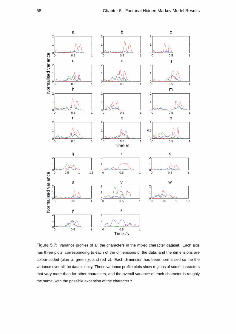
58 Chapter 5. Factorial Hidden Markov Model Results
0 0.5 10
1
2a
0 0.5 10
1
2b
0 0.5 10
1
2c
0 0.5 10
1
2d
Nor
mal
ised
var
ianc
e
0 0.5 10
1
2e
0 0.5 10
1
2g
0 0.5 10
1
2h
0 0.5 10
1
2l
0 0.5 10
1
2m
0 0.5 10
1
2n
0 0.5 10
1
2o
Time /s0 0.5 1
0
0.5
1p
0 0.5 1 1.50
1
2q
0 0.5 10
1
2r
0 0.5 10
1
2s
0 0.5 10
1
2u
Nor
mal
ised
var
ianc
e
0 0.5 10
1
2v
0 0.5 1 1.50
1
2w
0 0.5 10
1
2y
0 0.5 10
2
4z
Time /s
Figure 5.7: Variance profiles of all the characters in the mixed character dataset. Each axis
has three plots, corresponding to each of the dimensions of the data, and the dimensions are
colour-coded (blue=x, green=y, and red=z). Each dimension has been normalised so the the
variance over all the data is unity. These variance profile plots show regions of some characters
that vary more than for other characters, and the overall variance of each character is roughly
the same, with the possible exception of the character z.
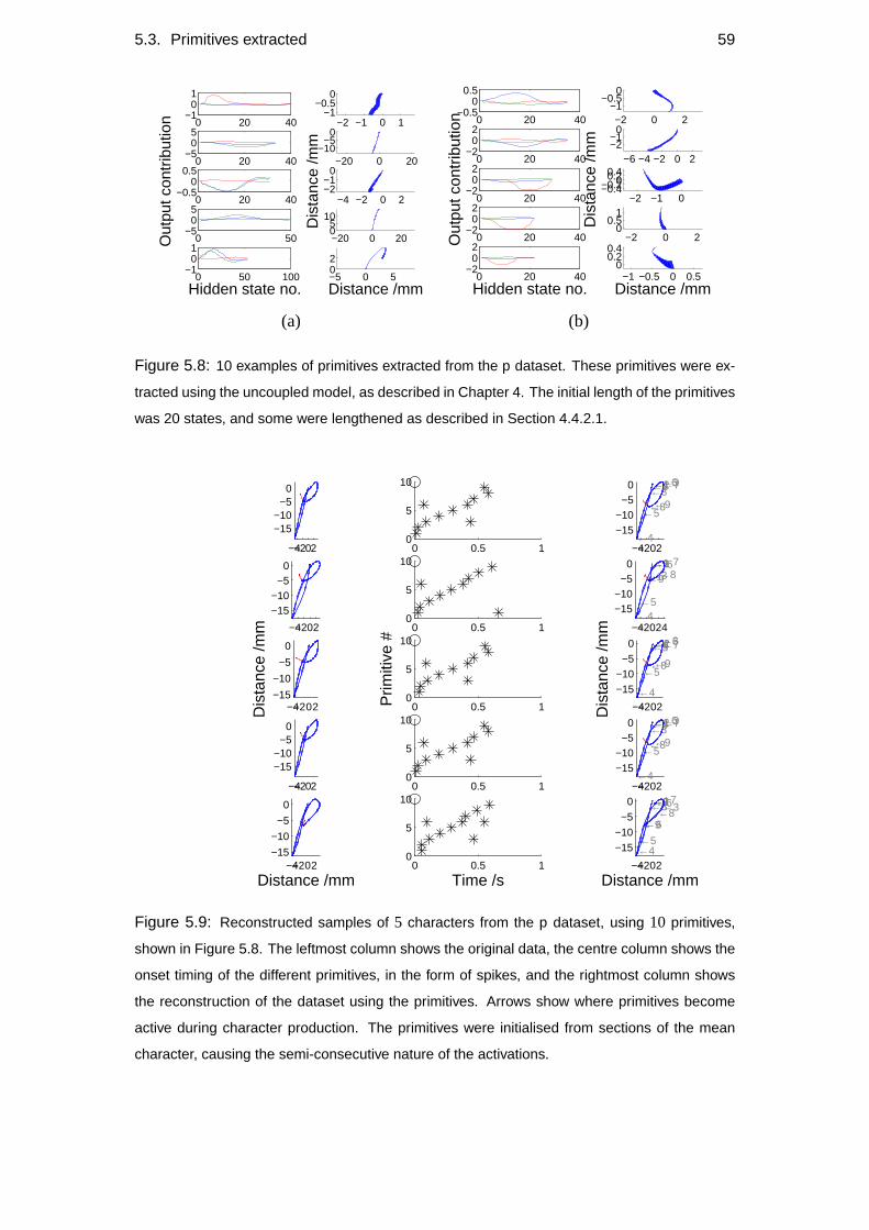
5.3. Primitives extracted 59
0 20 40−1
01
−2 −1 0 1−1
−0.50
0 20 40−5
05
−20 0 20−10
−50
0 20 40−0.5
00.5
Out
put c
ontr
ibut
ion
−4 −2 0 2−2−1
0
Dis
tanc
e /m
m
0 50−5
05
−20 0 2005
10
0 50 100−1
01
Hidden state no.−5 0 502
Distance /mm
0 20 40−0.5
00.5
−2 0 2−1
−0.50
0 20 40−2
02
−6 −4 −2 0 2−2−1
0
0 20 40−2
02
Out
put c
ontr
ibut
ion
−2 −1 0−0.4−0.20
0.20.4
Dis
tanc
e /m
m
0 20 40−2
02
−2 0 20
0.51
0 20 40−2
02
Hidden state no.−1 −0.5 0 0.5
00.20.4
Distance /mm
(a) (b)
Figure 5.8: 10 examples of primitives extracted from the p dataset. These primitives were ex-
tracted using the uncoupled model, as described in Chapter 4. The initial length of the primitives
was 20 states, and some were lengthened as described in Section 4.4.2.1.
−4−202
−15−10
−50
0 0.5 10
5
10
−4−202
−15−10
−50 ←1←2
←3←3
←4
←5
←6←6←7
←8←9
−4−202
−15−10
−50
0 0.5 10
5
10
−4−2024
−15−10
−50 ←1
←1←2←3
←4←5
←6←6←7←8←9
−4−202−15
−10
−5
0
Dis
tanc
e /m
m
0 0.5 10
5
10
Prim
itive
#
−4−202
−15−10
−50 ←1←2←3
←3
←4
←5
←6←6←7
←8←9
Dis
tanc
e /m
m
−4−202
−15−10
−50
0 0.5 10
5
10
−4−202
−15−10
−50 ←1←2
←3←3
←4
←5
←6←6←7
←8←9
−4−202−15
−10
−5
0
Distance /mm0 0.5 1
0
5
10
Time /s−4−202
−15−10
−5
0 ←1←2←3←3
←4←5
←6←6
←6
←7←8
←9
Distance /mm
Figure 5.9: Reconstructed samples of 5 characters from the p dataset, using 10 primitives,
shown in Figure 5.8. The leftmost column shows the original data, the centre column shows the
onset timing of the different primitives, in the form of spikes, and the rightmost column shows
the reconstruction of the dataset using the primitives. Arrows show where primitives become
active during character production. The primitives were initialised from sections of the mean
character, causing the semi-consecutive nature of the activations.
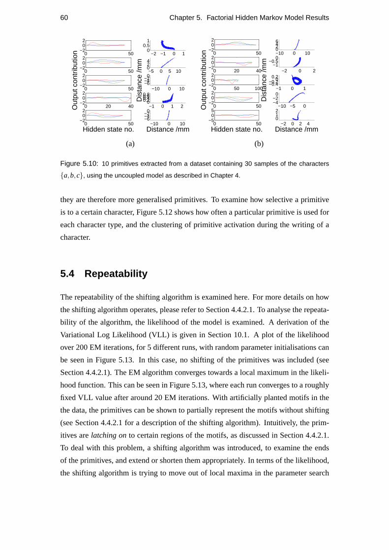
60 Chapter 5. Factorial Hidden Markov Model Results
0 50−2
02
−2 −1 0 10
0.51
0 50−2
02
−5 0 5 10024
0 50−2
02
Out
put c
ontr
ibut
ion
−10 0 10−6−4−20
Dis
tanc
e /m
m
0 20 40−2
02
−1 0 1 200.20.40.60.8
0 50−2
02
Hidden state no.−10 0 10
−6−4−20
Distance /mm
0 50−2
02
−10 0 100246
0 20 40−2
02
−2 0 2−1
−0.50
0 50 100−2
02
Out
put c
ontr
ibut
ion
−1 0 1−0.4−0.20
0.2
Dis
tanc
e /m
m
0 50−2
02
−10 −5 0−4−2
0
0 50−5
05
Hidden state no.−2 0 2 4
012
Distance /mm
(a) (b)
Figure 5.10: 10 primitives extracted from a dataset containing 30 samples of the characters
{a,b,c}, using the uncoupled model as described in Chapter 4.
they are therefore more generalised primitives. To examine how selective a primitive
is to a certain character, Figure 5.12 shows how often a particular primitive is used for
each character type, and the clustering of primitive activation during the writing of a
character.
5.4 Repeatability
The repeatability of the shifting algorithm is examined here. For more details on how
the shifting algorithm operates, please refer to Section 4.4.2.1. To analyse the repeata-
bility of the algorithm, the likelihood of the model is examined. A derivation of the
Variational Log Likelihood (VLL) is given in Section 10.1. A plot of the likelihood
over 200 EM iterations, for 5 different runs, with random parameter initialisations can
be seen in Figure 5.13. In this case, no shifting of the primitives was included (see
Section 4.4.2.1). The EM algorithm converges towards a local maximum in the likeli-
hood function. This can be seen in Figure 5.13, where each run converges to a roughly
fixed VLL value after around 20 EM iterations. With artificially planted motifs in the
the data, the primitives can be shown to partially represent the motifs without shifting
(see Section 4.4.2.1 for a description of the shifting algorithm). Intuitively, the prim-
itives arelatching onto certain regions of the motifs, as discussed in Section 4.4.2.1.
To deal with this problem, a shifting algorithm was introduced, to examine the ends
of the primitives, and extend or shorten them appropriately. In terms of the likelihood,
the shifting algorithm is trying to move out of local maxima in the parameter search
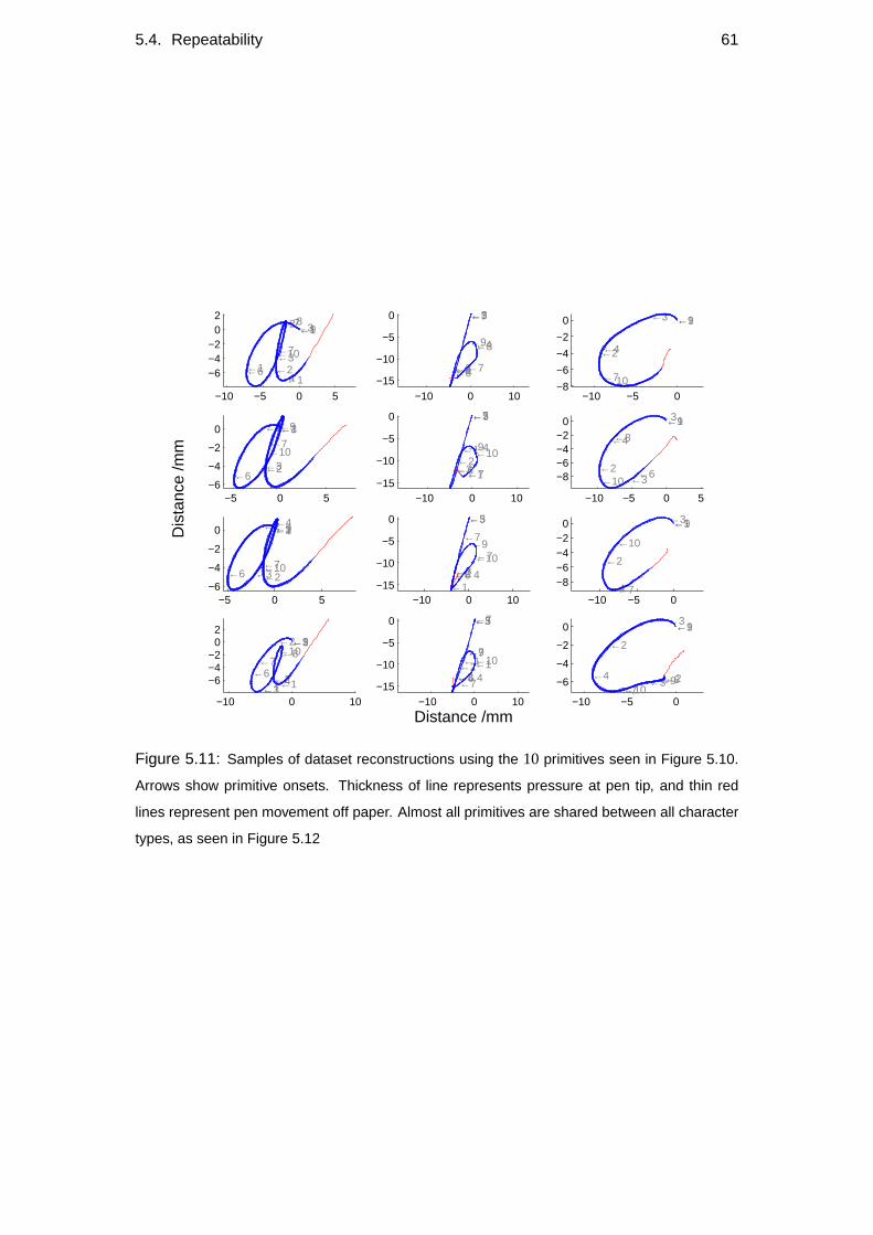
5.4. Repeatability 61
−10 −5 0 5
−6−4−2
02
←1
←1←1
←2
←2
←3
←3
←4←6
←7
←7
←8←9
←10
−10 0 10−15
−10
−5
0
←1←2
←3
←3
←4
←5
←6
←7
←7
←8←9
−10 −5 0−8
−6
−4
−2
0 ←1
←2
←3
←4
←7
←9
←10
−5 0 5−6
−4
−2
0 ←1←2
←2
←3
←3←6
←7
←9
←10
−10 0 10−15
−10
−5
0
←1
←1←2
←3
←3
←4
←5
←6
←7
←7
←9←10
−10 −5 0 5
−8−6−4−2
0 ←1
←2
←3
←3
←4
←6
←8
←9
←10
−5 0 5−6
−4
−2
0 ←1←2
←2
←3
←3
←4
←6←7
←9
←10
Dis
tanc
e /m
m
−10 0 10−15
−10
−5
0
←1←2
←3
←3←4
←5
←6
←7
←7←9←10
−10 −5 0
−8−6−4−2
0 ←1
←2
←3
←4←7
←9
←10
−10 0 10
−6−4−2
02
←1
←1←1
←2
←2
←3
←3←4
←6←7
←8←9
←10
−10 0 10−15
−10
−5
0
←1←1←2
←3
←3←4
←5
←6
←7
←7
←7
←9←10
Distance /mm−10 −5 0
−6
−4
−2
0 ←1
←2
←2
←3
←3←4 ←6
←7
←9
←9←10
Figure 5.11: Samples of dataset reconstructions using the 10 primitives seen in Figure 5.10.
Arrows show primitive onsets. Thickness of line represents pressure at pen tip, and thin red
lines represent pen movement off paper. Almost all primitives are shared between all character
types, as seen in Figure 5.12
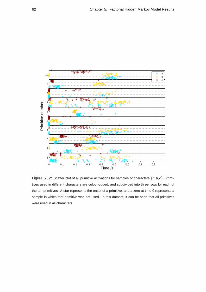
62 Chapter 5. Factorial Hidden Markov Model Results
0 0.1 0.2 0.3 0.4 0.5 0.6 0.7 0.8
1
2
3
4
5
6
7
8
9
10
Time /s
Prim
itive
num
ber
abc
Figure 5.12: Scatter plot of all primitive activations for samples of characters {a,b,c}. Primi-
tives used in different characters are colour-coded, and subdivided into three rows for each of
the ten primitives. A star represents the onset of a primitive, and a zero at time 0 represents a
sample in which that primitive was not used. In this dataset, it can be seen that all primitives
were used in all characters.
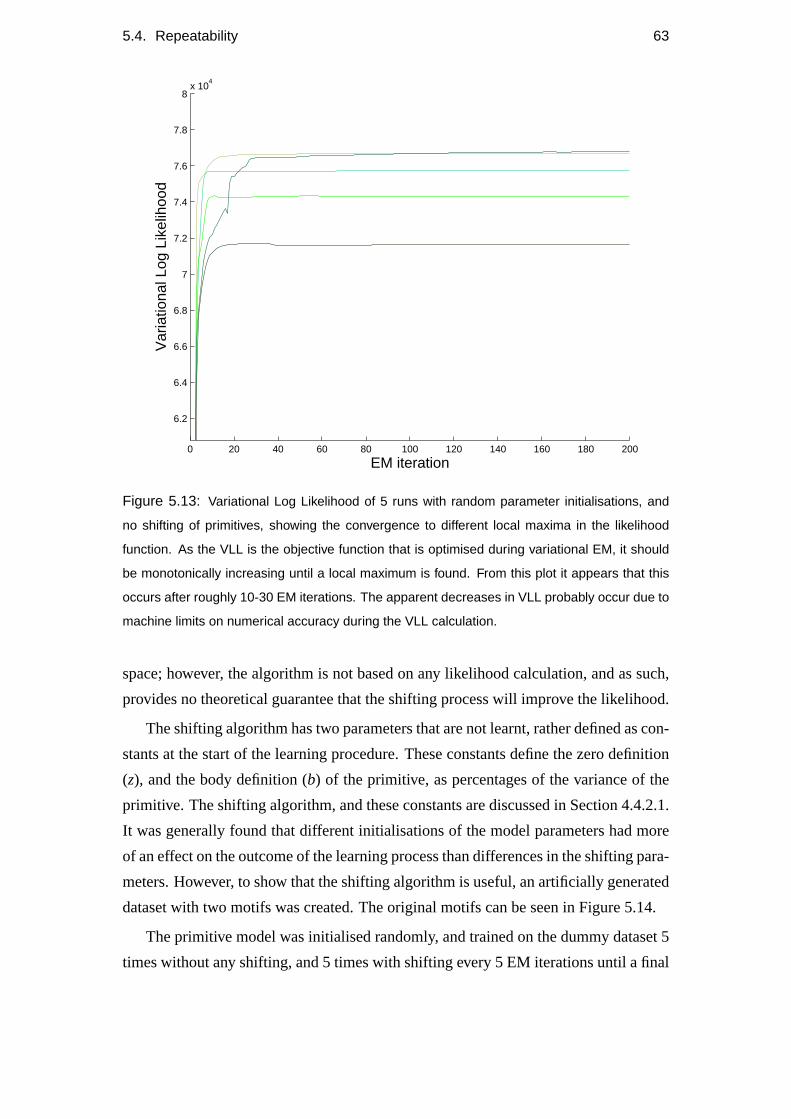
5.4. Repeatability 63
0 20 40 60 80 100 120 140 160 180 200
6.2
6.4
6.6
6.8
7
7.2
7.4
7.6
7.8
8x 10
4
EM iteration
Var
iatio
nal L
og L
ikel
ihoo
d
Figure 5.13: Variational Log Likelihood of 5 runs with random parameter initialisations, and
no shifting of primitives, showing the convergence to different local maxima in the likelihood
function. As the VLL is the objective function that is optimised during variational EM, it should
be monotonically increasing until a local maximum is found. From this plot it appears that this
occurs after roughly 10-30 EM iterations. The apparent decreases in VLL probably occur due to
machine limits on numerical accuracy during the VLL calculation.
space; however, the algorithm is not based on any likelihood calculation, and as such,
provides no theoretical guarantee that the shifting process will improve the likelihood.
The shifting algorithm has two parameters that are not learnt, rather defined as con-
stants at the start of the learning procedure. These constants define the zero definition
(z), and the body definition (b) of the primitive, as percentages of the variance of the
primitive. The shifting algorithm, and these constants are discussed in Section 4.4.2.1.
It was generally found that different initialisations of the model parameters had more
of an effect on the outcome of the learning process than differences in the shifting para-
meters. However, to show that the shifting algorithm is useful, an artificially generated
dataset with two motifs was created. The original motifs can be seen in Figure 5.14.
The primitive model was initialised randomly, and trained on the dummy dataset 5
times without any shifting, and 5 times with shifting every 5 EM iterations until a final
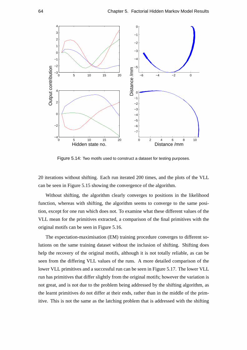
64 Chapter 5. Factorial Hidden Markov Model Results
0 5 10 15 20−3
−2
−1
0
1
2
3
4
Out
put c
ontr
ibut
ion
−6 −4 −2 0
−5
−4
−3
−2
−1
0
Dis
tanc
e /m
m
0 5 10 15 20−4
−2
0
2
4
Hidden state no.0 2 4 6 8 10
−7
−6
−5
−4
−3
−2
−1
0
Distance /mm
Figure 5.14: Two motifs used to construct a dataset for testing purposes.
20 iterations without shifting. Each run iterated 200 times, and the plots of the VLL
can be seen in Figure 5.15 showing the convergence of the algorithm.
Without shifting, the algorithm clearly converges to positions in the likelihood
function, whereas with shifting, the algorithm seems to converge to the same posi-
tion, except for one run which does not. To examine what these different values of the
VLL mean for the primitives extracted, a comparison of the final primitives with the
original motifs can be seen in Figure 5.16.
The expectation-maximisation (EM) training procedure converges to different so-
lutions on the same training dataset without the inclusion of shifting. Shifting does
help the recovery of the original motifs, although it is not totally reliable, as can be
seen from the differing VLL values of the runs. A more detailed comparison of the
lower VLL primitives and a successful run can be seen in Figure 5.17. The lower VLL
run has primitives that differ slightly from the original motifs; however the variation is
not great, and is not due to the problem being addressed by the shifting algorithm, as
the learnt primitives do not differ at their ends, rather than in the middle of the prim-
itive. This is not the same as the latching problem that is addressed with the shifting
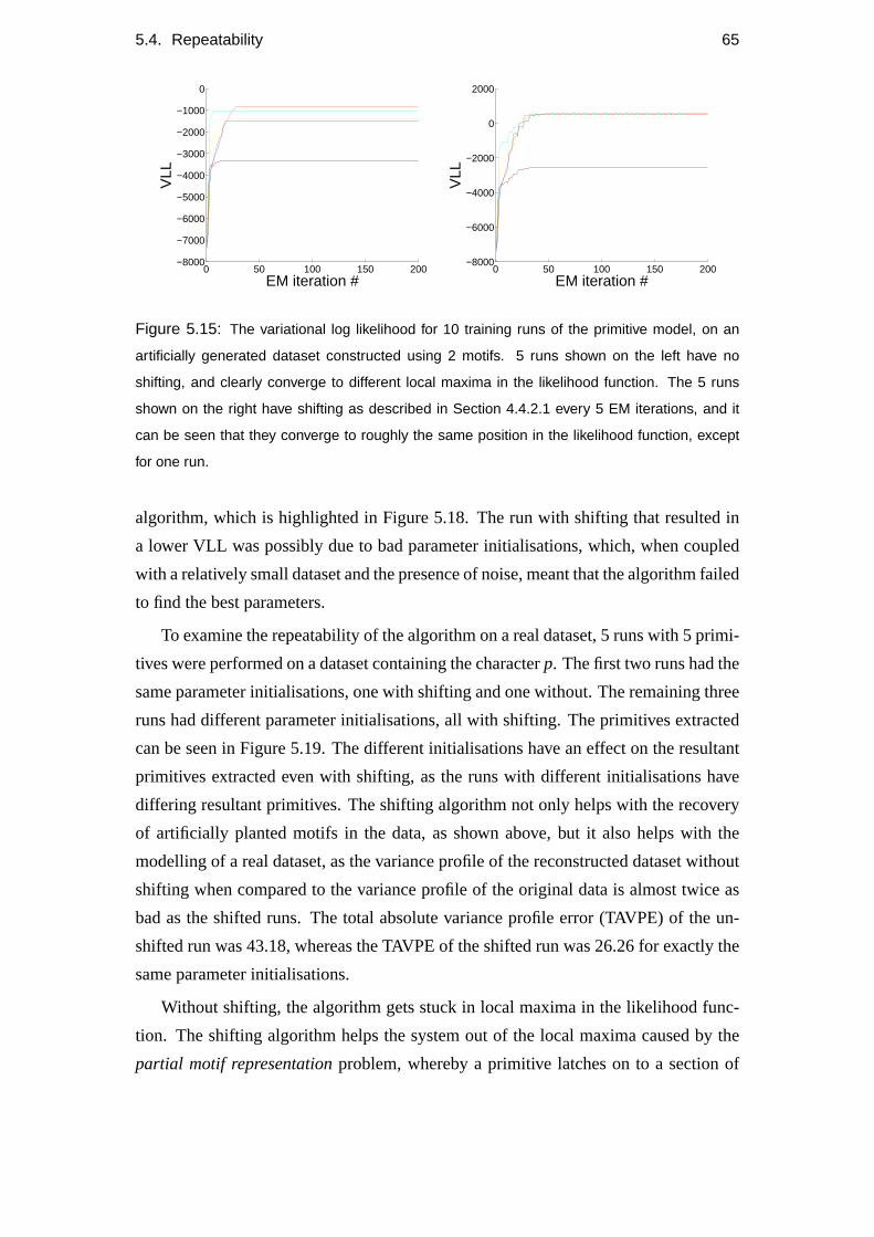
5.4. Repeatability 65
0 50 100 150 200−8000
−7000
−6000
−5000
−4000
−3000
−2000
−1000
0
EM iteration #
VLL
0 50 100 150 200−8000
−6000
−4000
−2000
0
2000
EM iteration #
VLL
Figure 5.15: The variational log likelihood for 10 training runs of the primitive model, on an
artificially generated dataset constructed using 2 motifs. 5 runs shown on the left have no
shifting, and clearly converge to different local maxima in the likelihood function. The 5 runs
shown on the right have shifting as described in Section 4.4.2.1 every 5 EM iterations, and it
can be seen that they converge to roughly the same position in the likelihood function, except
for one run.
algorithm, which is highlighted in Figure 5.18. The run with shifting that resulted in
a lower VLL was possibly due to bad parameter initialisations, which, when coupled
with a relatively small dataset and the presence of noise, meant that the algorithm failed
to find the best parameters.
To examine the repeatability of the algorithm on a real dataset, 5 runs with 5 primi-
tives were performed on a dataset containing the characterp. The first two runs had the
same parameter initialisations, one with shifting and one without. The remaining three
runs had different parameter initialisations, all with shifting. The primitives extracted
can be seen in Figure 5.19. The different initialisations have an effect on the resultant
primitives extracted even with shifting, as the runs with different initialisations have
differing resultant primitives. The shifting algorithm not only helps with the recovery
of artificially planted motifs in the data, as shown above, but it also helps with the
modelling of a real dataset, as the variance profile of the reconstructed dataset without
shifting when compared to the variance profile of the original data is almost twice as
bad as the shifted runs. The total absolute variance profile error (TAVPE) of the un-
shifted run was 43.18, whereas the TAVPE of the shifted run was 26.26 for exactly the
same parameter initialisations.
Without shifting, the algorithm gets stuck in local maxima in the likelihood func-
tion. The shifting algorithm helps the system out of the local maxima caused by the
partial motif representationproblem, whereby a primitive latches on to a section of
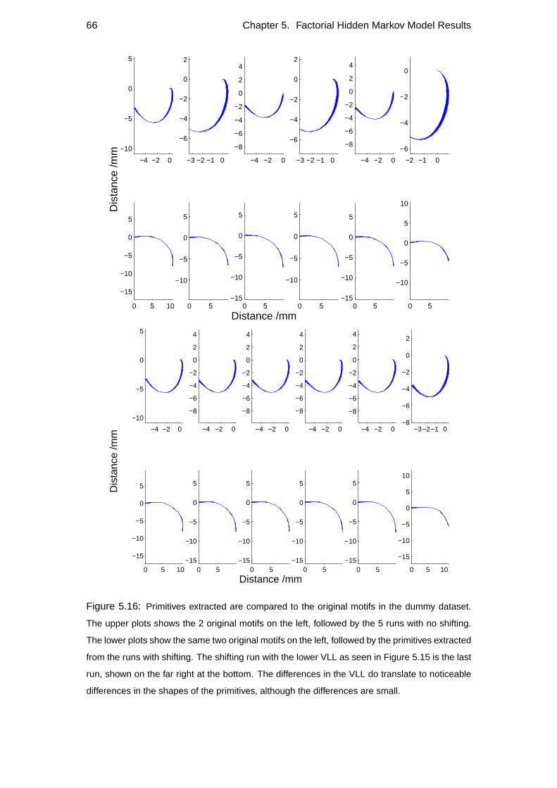
66 Chapter 5. Factorial Hidden Markov Model Results
−4 −2 0
−10
−5
0
5
Dis
tanc
e /m
m
0 5 10
−15
−10
−5
0
5
−3 −2 −1 0
−6
−4
−2
0
2
0 5
−10
−5
0
5
−4 −2 0
−8
−6
−4
−2
0
2
4
0 5−15
−10
−5
0
5
Distance /mm
−3 −2 −1 0
−6
−4
−2
0
2
0 5
−10
−5
0
5
−4 −2 0
−8
−6
−4
−2
0
2
4
0 5−15
−10
−5
0
5
−2 −1 0
−6
−4
−2
0
0 5
−10
−5
0
5
10
−4 −2 0
−10
−5
0
5
Dis
tanc
e /m
m
0 5 10
−15
−10
−5
0
5
−4 −2 0
−8
−6
−4
−2
0
2
4
0 5−15
−10
−5
0
5
−4 −2 0
−8
−6
−4
−2
0
2
4
0 5−15
−10
−5
0
5
Distance /mm
−4 −2 0
−8
−6
−4
−2
0
2
4
0 5−15
−10
−5
0
5
−4 −2 0
−8
−6
−4
−2
0
2
4
0 5−15
−10
−5
0
5
−3−2−1 0−8
−6
−4
−2
0
2
0 5 10
−15
−10
−5
0
5
10
Figure 5.16: Primitives extracted are compared to the original motifs in the dummy dataset.
The upper plots shows the 2 original motifs on the left, followed by the 5 runs with no shifting.
The lower plots show the same two original motifs on the left, followed by the primitives extracted
from the runs with shifting. The shifting run with the lower VLL as seen in Figure 5.15 is the last
run, shown on the far right at the bottom. The differences in the VLL do translate to noticeable
differences in the shapes of the primitives, although the differences are small.
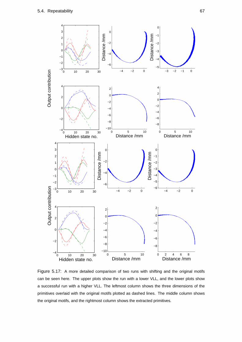
5.4. Repeatability 67
0 10 20 30−3
−2
−1
0
1
2
3
4
Out
put c
ontr
ibut
ion −4 −2 0
−6
−4
−2
0
Dis
tanc
e /m
m
−3 −2 −1 0−5
−4
−3
−2
−1
0
Dis
tanc
e /m
m
0 10 20 30−4
−2
0
2
4
Hidden state no.0 5 10
−10
−8
−6
−4
−2
0
2
Distance /mm0 5 10
−8
−6
−4
−2
0
2
4
Distance /mm
0 10 20 30−3
−2
−1
0
1
2
3
4
Out
put c
ontr
ibut
ion
−4 −2 0
−6
−4
−2
0
Dis
tanc
e /m
m
−4 −2 0−6
−5
−4
−3
−2
−1
0D
ista
nce
/mm
0 10 20 30−4
−2
0
2
4
Hidden state no.0 5 10
−10
−8
−6
−4
−2
0
2
Distance /mm0 2 4 6 8
−8
−6
−4
−2
0
2
Distance /mm
Figure 5.17: A more detailed comparison of two runs with shifting and the original motifs
can be seen here. The upper plots show the run with a lower VLL, and the lower plots show
a successful run with a higher VLL. The leftmost column shows the three dimensions of the
primitives overlaid with the original motifs plotted as dashed lines. The middle column shows
the original motifs, and the rightmost column shows the extracted primitives.
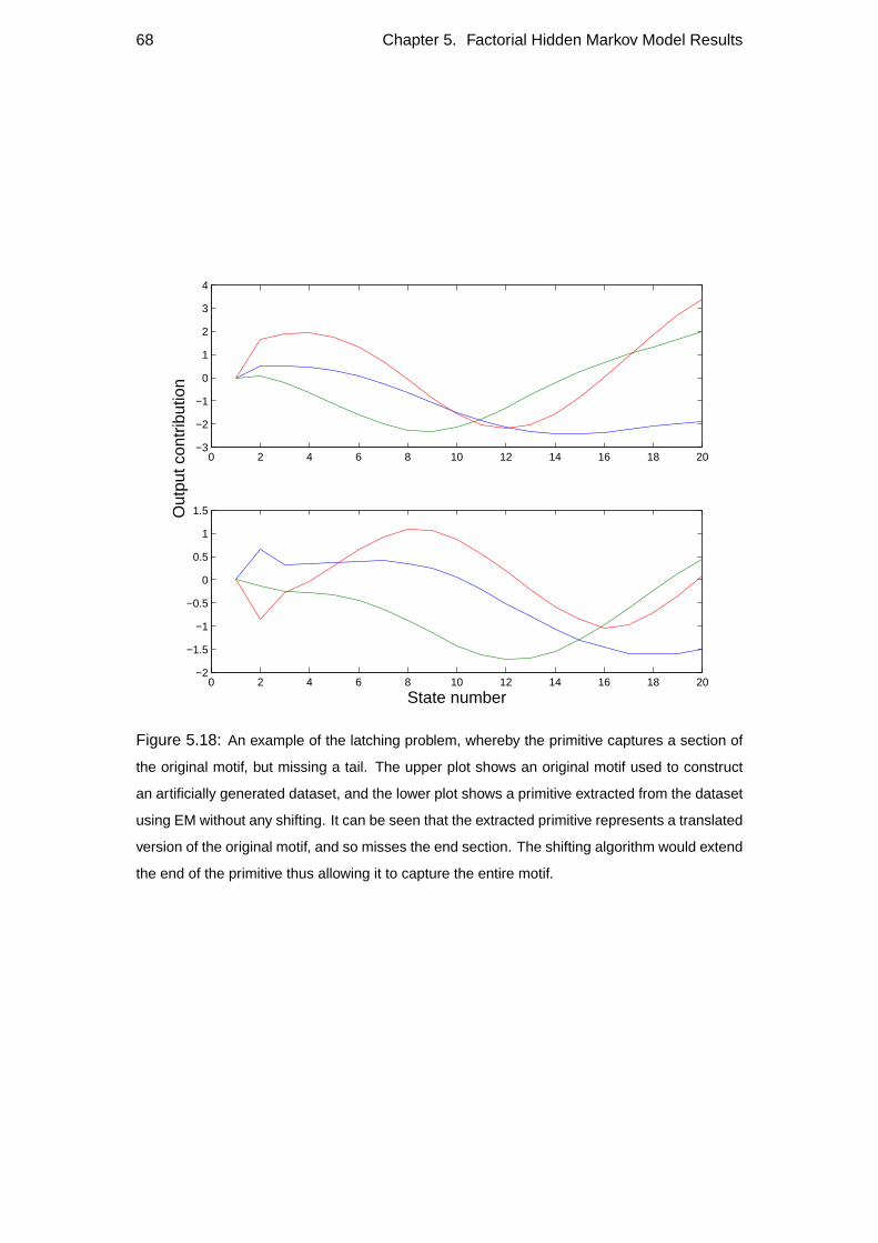
68 Chapter 5. Factorial Hidden Markov Model Results
0 2 4 6 8 10 12 14 16 18 20−3
−2
−1
0
1
2
3
4
0 2 4 6 8 10 12 14 16 18 20−2
−1.5
−1
−0.5
0
0.5
1
1.5
State number
Out
put c
ontr
ibut
ion
Figure 5.18: An example of the latching problem, whereby the primitive captures a section of
the original motif, but missing a tail. The upper plot shows an original motif used to construct
an artificially generated dataset, and the lower plot shows a primitive extracted from the dataset
using EM without any shifting. It can be seen that the extracted primitive represents a translated
version of the original motif, and so misses the end section. The shifting algorithm would extend
the end of the primitive thus allowing it to capture the entire motif.

5.4. Repeatability 69
−2 0 2 40
5
−1.5−1−0.5 0 0.5−1.5
−1−0.5
0
−2 0 2 4 6 802468
Dis
tanc
e /m
m
−5 0 5−10
−5
0
−4 −2 0 2
−5
0
0 2 40123
−2 −1 0−2
−1
0
−5 0 5 100
5
10
−10 −5 0 5
−10
−5
0
−2 −1 0 1
−3
−2
−1
0
−4−2 0 2 4 60
5
−2 0 2−4
−2
0
−5 0 5 100
5
10
15
−5 0 5
−10
−5
0
−1.5−1−0.5 0 0.50
0.5
1
1.5
Distance /mm
0 20
1
2
−4 −2 0−3
−2
−1
0
−5 0 50
5
10
−10 −5 0 5
−10
−5
0
−1 0 1 2 30123
−4−2 0 2 4 6 80
5
10
−4 −2 0
−3−2−1
0
0 2 40
2
−10 −5 0 5−15
−10
−5
0
−2 0 20
2
4
Figure 5.19: Five primitives were trained on a dataset containing the character p multiple times
with different initialisations. Each column represents the resultant primitives of a separate run.
The first 3 leftmost columns are the results of 3 runs with different parameter initialisations,
showing certain similarities in the primitives extracted. The 2 rightmost columns show two runs
with identical parameter initialisations, where one run has shifting and one without, showing the
effect of shifting on otherwise identical runs.
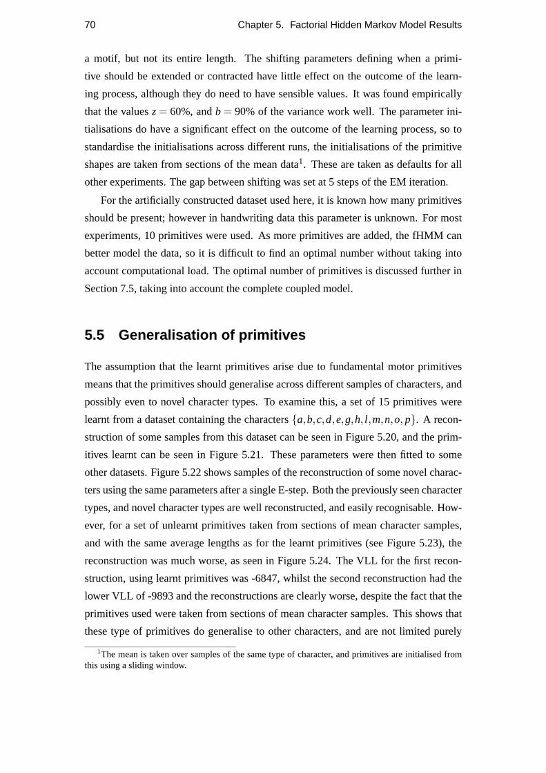
70 Chapter 5. Factorial Hidden Markov Model Results
a motif, but not its entire length. The shifting parameters defining when a primi-
tive should be extended or contracted have little effect on the outcome of the learn-
ing process, although they do need to have sensible values. It was found empirically
that the valuesz= 60%, andb = 90% of the variance work well. The parameter ini-
tialisations do have a significant effect on the outcome of the learning process, so to
standardise the initialisations across different runs, the initialisations of the primitive
shapes are taken from sections of the mean data1. These are taken as defaults for all
other experiments. The gap between shifting was set at 5 steps of the EM iteration.
For the artificially constructed dataset used here, it is known how many primitives
should be present; however in handwriting data this parameter is unknown. For most
experiments, 10 primitives were used. As more primitives are added, the fHMM can
better model the data, so it is difficult to find an optimal number without taking into
account computational load. The optimal number of primitives is discussed further in
Section 7.5, taking into account the complete coupled model.
5.5 Generalisation of primitives
The assumption that the learnt primitives arise due to fundamental motor primitives
means that the primitives should generalise across different samples of characters, and
possibly even to novel character types. To examine this, a set of 15 primitives were
learnt from a dataset containing the characters{a,b,c,d,e,g,h, l ,m,n,o, p}. A recon-
struction of some samples from this dataset can be seen in Figure 5.20, and the prim-
itives learnt can be seen in Figure 5.21. These parameters were then fitted to some
other datasets. Figure 5.22 shows samples of the reconstruction of some novel charac-
ters using the same parameters after a single E-step. Both the previously seen character
types, and novel character types are well reconstructed, and easily recognisable. How-
ever, for a set of unlearnt primitives taken from sections of mean character samples,
and with the same average lengths as for the learnt primitives (see Figure 5.23), the
reconstruction was much worse, as seen in Figure 5.24. The VLL for the first recon-
struction, using learnt primitives was -6847, whilst the second reconstruction had the
lower VLL of -9893 and the reconstructions are clearly worse, despite the fact that the
primitives used were taken from sections of mean character samples. This shows that
these type of primitives do generalise to other characters, and are not limited purely
1The mean is taken over samples of the same type of character, and primitives are initialised fromthis using a sliding window.
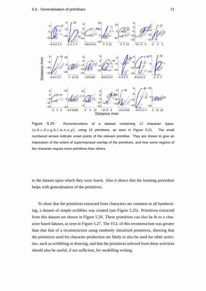
5.5. Generalisation of primitives 71
−6−4−2 0 2
−10
−5
0 ←1
←2
←3
←3←5
←6
←9←10
←10
←11
←11←13
←15
Dis
tanc
e /m
m−2 0 2 4
−10
−5
0
←2
←2
←3
←3
←5
←7
←7←7
←8
←9
←9
←10
←10
←11
←12
←12←15
−8−6−4−2 0 2
−10
−5
0
5
←2
←3←4←9 ←10
←10
←11
←12←13
←14←15
←15
0 5 10−10
0
10
20
←1←2←3←3←3
←4
←5←5←6
←6
←7←9
←10
←11
←13←14
0 5 10
−10
0
10
←1←1
←2
←3
←3
←4←4
←4
←5
←6←7
←8←9←10
←10←11←12
←13
←15←15
−10 −5 0
−15
−10
−5
0
5
←1←1
←2
←3←3←4←6←7←8←8
←9←9
←9
←10←10
←10
←11←11←12
←14
←14←15
←15
−5 0 5
−15
−10
−5
0 ←1
←2
←2
←3
←3←3
←5←6←6
←7
←9
←10
←10
←11
←11←12←13
←15
−6−4−2 0 2
−15
−10
−5
0 ←1
←2
←2
←3
←3
←6
←7
←9
←10←11
←12←13←15
0 10 20
−20
0
20
←1 ←2←3←3←4←5←5←5←6
←7←9←9←10
←10←10←11←12
←12←13
←13
−202468
−15
−10
−5
0
5
←2
←2
←3←3←5
←6
←7←7
←9←9
←10
←10
←11←12←12←13
←14
←15
−8−6−4−2 0 2
−10
−5
0
5
←1
←2
←3
←3←3
←4←4
←6←6
←7
←9←10
←10←11
←13
←14
←14←15
−6−4−2 0
−10
−5
0 ←1
←1←2
←2←2
←3←3
←5
←6
←7←8←9
←9
←10←10←11
←11
←11
←12
←12
←14−8−6−4−2 0
−15
−10
−5
0 ←1
←1←2
←3
←3
←4
←4
←5
←10
←10←11←13
←14
←15
−2 0 2
−10
−5
0 ←1
←2←2
←3
←3
←6
←7
←8
←9
←9←9
←10
←10←11←12
←14
←15
−5 0 5−15
−10
−5
0
5
←1
←2
←3←4
←6
←9←10
←10←13
←14
−5 0 51015−20
0
20
←2←2←3←3←3←4
←4←4
←5 ←5←6←7←7←9
←9←10←12←12←13←14←14
←14
0 5 10
−5
0
5
10
←1←2←3
←3←4
←5←6←7
←7←9←10
←11←13←14
←15←15
−10−5 0
−15
−10
−5
0
5
←1
←2←2
←3←3←4←7
←8←9
←9
←10
←10
←11
←12
←14←14
←14
←15
Distance /mm−2 0 2 4 6 8
−15
−10
−5
0
←2
←2
←3
←3←5
←7
←7
←9
←9
←10
←10
←11←12
←12←13←15
−4−2 0 2 4
−15
−10
−5
0 ←1
←2
←2
←3
←3
←4
←5
←7←10←11
←11
←12←13←15←15
0 10 20
−20
0
20
←1←2←3←3←3←4
←5←5←6←7←7←9←9
←10←10
←12←12←13←13←15
Figure 5.20: Reconstructions of a dataset containing 12 character types:
{a,b,c,d,e,g,h, l ,m,n,o, p}, using 15 primitives, as seen in Figure 5.21. The small
numbered arrows indicate onset points of the relevant primitive. They are shown to give an
impression of the extent of superimposed overlap of the primitives, and how some regions of
the character require more primitives than others.
to the dataset upon which they were learnt. Also it shows that the learning procedure
helps with generalisation of the primitives.
To show that the primitives extracted from characters are common to all handwrit-
ing, a dataset of simple scribbles was created (see Figure 5.25). Primitives extracted
from this dataset are shown in Figure 5.26. These primitives can also be fit to a char-
acter based dataset, as seen in Figure 5.27. The VLL of this reconstruction was greater
than that that of a reconstruction using randomly initialised primitives, showing that
the primitives used for character production are likely to also be used for other activi-
ties, such as scribbling or drawing, and that the primitives inferred from these activities
should also be useful, if not sufficient, for modelling writing.

72 Chapter 5. Factorial Hidden Markov Model Results
−0.8−0.6−0.4−0.200.20
0.51
00.511.5012
Dis
tanc
e /m
m
−4−2 0−6−4−2
0
0123−3−2−10
1
024605
0 2 4024
−1 0 1−3−2−1
0
−4−20−4−2
02
0123−10
123
−3−2−101−6−4−2
0
−2−10−3−2−1
0
−0.100.1−0.2−0.1
00.1
0123024
Distance /mm−2−10
024
−1012024
0 20 40−2
0
2
0 10 20−5
0
5
Out
put c
ontr
ibut
ion
0 50−2
0
2
0 20 40−2
0
2
0 20 40−2
0
2
0 20 40−2
0
2
0 20 40−1
0
1
0 50−2
0
2
0 20 40−2
0
2
0 20 40−2
0
2
0 50−1
0
1
0 20 40−2
0
2
0 20 40−5
0
5
Hidden state no.0 20 40
−1
0
1
0 20 40−1
0
1
Figure 5.21: Primitives learnt from varied dataset, containing 12 character types. Reconstruc-
tions of the dataset can be seen in Figure 5.20.
−6−4−2 0 2 4
−8−6−4−2
0 ←1
←2
←2
←3
←3
←4←4
←5←7
←7←8
←9
←10←11
←12←12
←14
←15←15
−10 −5 0 5−15
−10
−5
0 ←1
←1←2
←3
←3
←4
←4←5
←7←8
←8←9←9
←10
←10←10
←11
←11←12
←15
←15
←15
−8 −6 −4 −2 0−6−4−2
02
←1
←2
←2
←3←4
←6←7←8←9
←10
←11
←12 ←12
←14
←15
−5 0 5 10
−5
0
5
←1
←1←2
←2←3←3
←4
←4
←5 ←5←6
←7
←7
←7
←8←8←9←9←10←11
←12 ←12
←15
−4−2 0 2 4 6 8
−5
0
5
←1←1
←2
←3
←4
←4
←5
←5
←7
←7
←8
←8
←9
←10
←11←12
←15
−10 −5 0−15
−10
−5
0 ←1
←1←2
←3←3←4←6
←7←8←10←11←11←12
←13
←14
←15
Dis
tanc
e /m
m
0 5 10
−10
−5
0
←2
←3
←3
←4
←4
←5←5
←7
←7 ←7
←8
←9
←11←12
←15
−5 0 5
−10
−5
0 ←1
←1←2
←2
←3←4←7
←8
←9
←10
←12
←15
0 5 10
−10
−5
0 ←1
←1←2
←3
←3
←4 ←4←4
←5 ←6←6
←7←7
←7
←8
←8←9 ←9
←9←10
←10
←11
←11←12
←15
←15←15
0 5 10 15
−10
−5
0
5
←2
←2←3
←3
←4
←4←5←5
←6←6←7
←7←8←9 ←9
←10
←11←11
←12
←12←12
←15
−6−4−2 0 2 4−8−6−4−2
02
←1←2 ←3
←3
←4←4
←5
←7←7←10 ←11
←11
←12←13←14
←15
−10 −5 0 5
−15
−10
−5
0
←1
←2
←3←3←4←4
←5
←6
←7←7
←7←8←8←9←9
←10
←11
←11←12
←12
←12
←14←14
−5 0 5 10−20
−10
0 ←1←1
←2←2
←3←3
←3
←4←4
←4←5
←6←7
←7
←10←11←11
←12
←15
←15
−5 0 5 10
−15
−10
−5
0 ←1
←1
←2←2
←3
←3
←4←4
←5
←6
←7
←8←9
←10←11
←11
←12
←12←12←13
←15−10 −5 0
−10
−5
0 ←1
←2
←3
←3
←4←6←7
←7
←8←9
←11
←11
←12←14
←14
0 5 10
−10
−5
0 ←1
←1←2
←3
←3
←4←4
←5←6
←7
←7←8
←9
←9
←10
←10←11
←12←13
←15
←15
0 5 10
−10
−5
0
←1←2←2
←3
←3
←4
←4
←5
←7
←8
←9
←9
←10←11
←12
←12
←15
←15
−4−2 0 2 4 6 8−8−6−4−2
024
←1←2
←2
←3
←4←4
←5←6←6
←7
←7
←8
←8←9←9
←10
←10←11
←12
←12←12
←12←14
←15
Distance /mm−10 0 10
−15
−10
−5
0 ←1
←2
←3←3
←4 ←4
←6
←7←7
←7
←8←10←11
←11←12←13←14
←15
0 5 10
−10
−5
0
←2
←3
←3
←4
←4←5
←6
←6
←7
←7←7
←9←10
←10
←11←11
←12←13
←14
Figure 5.22: Reconstructions of a novel dataset of 20 character types, containing 8 character
types not present in the training set. The primitives used can be seen in Figure 5.21.

5.5. Generalisation of primitives 73
−4−2 0−4−2
02
−8−6−4−202
−10−5
0
Dis
tanc
e /m
m0 5
−4−202468
0 5−2
024
0 50246
0 246−2
0246
−3−2−101−6−4−2
0
02468−5
05
−8−6−4−202−15−10
−50
0 2 4−4−2
02
−20246805
1015
−4−2 0
−5
0
0 50
5
10
Distance /mm0 2 4
−2024
−10−5 0−15−10
−50
0 20 40−2
0
2
0 20 40−5
0
5
Out
put c
ontr
ibut
ion
0 20 40−5
0
5
0 20 40−5
0
5
0 20 40−2
0
2
0 20 40−5
0
5
0 20 40−2
0
2
0 20 40−5
0
5
0 20 40−5
0
5
0 20 40−2
0
2
0 20 40−5
0
5
0 20 40−2
0
2
0 20 40−5
0
5
Hidden state no.0 20 40
−2
0
2
0 20 40−4
−2
0
Figure 5.23: Unlearnt set of primitives initialised from the complete dataset, containing 20char-
acter types. The length of each primitive is equal to the average lengths of the primitives seen
in Figure 5.21. It should be noted that the combined length of all the primitives is considerably
shorter than the combined length of all the character types.
−5 0 5
−10
−5
0 ←1
←5
←6
←7
←12
−15−10−5 0 5
−20
−10
0 ←1
←1
←2
←2
←5
←5
←6
−4 −2 0 2−6
−4
−2
0
2←1
←3
−5 0 5 10
0
5
10
15
←1
←2
←3
←5←110 5 10
−10
−5
0←1
←2
←3
←4←5
−15−10 −5 0 5
−15
−10
−5
0 ←1←1←2
←5
←12
←13
Dis
tanc
e /m
m
−2 0 2 4 6 8−5
0
5
←1
←1
←5
←5←6
←7
−10 −5 0 5
−15
−10
−5
0 ←1←2←5
←6←12
−5 0 5 10−20
−10
0 ←2
←2
←3
←5←14
0 10 20−10
0
10
←1←1←3
←5←5←5←7←7
←11
←12
−15−10−5 0 5
−20
−10
0 ←1
←1
←1
←4
←5
←6
←7
←7←9
−10 −5 0 5
−10
−5
0
5
←1←1
←2←5←5
←9
←11
←13
−5 0 5
−10
−5
0 ←1←2
←5
←13
←14
−10 0 10
−10
−5
0
5
←2←6
←7
←11−10 −5 0
−10
−5
0 ←1
←1
←5
←6
←7←12
←12
−10 −5 0 5−20
−10
0 ←1
←5←6
←7
←9←10
0 5 10
−10
−5
0 ←2←4←6←7
←11
←12
0 5 10
−10
−5
0←2
←3
←5
←7
Distance /mm−10 −5 0 5
−15
−10
−5
0 ←1←1←2
←5←7
←12
←13
−10 0 10−20
−10
0
←1
←4
←4
←5
←7
←9
←12
←12←13←14
Figure 5.24: Attempted reconstruction of character samples from the complete dataset con-
taining 20 character types, using 20 primitives taken from the dataset. This reconstruction is
produced after a single E-step, similar to the data shown in Figure 5.22. Comparison of the
reconstructed samples from these two datasets suggests that the learnt primitives generalise
better to novel character samples (Figure 5.22), than primitives taken from an average of the
data (This figure).
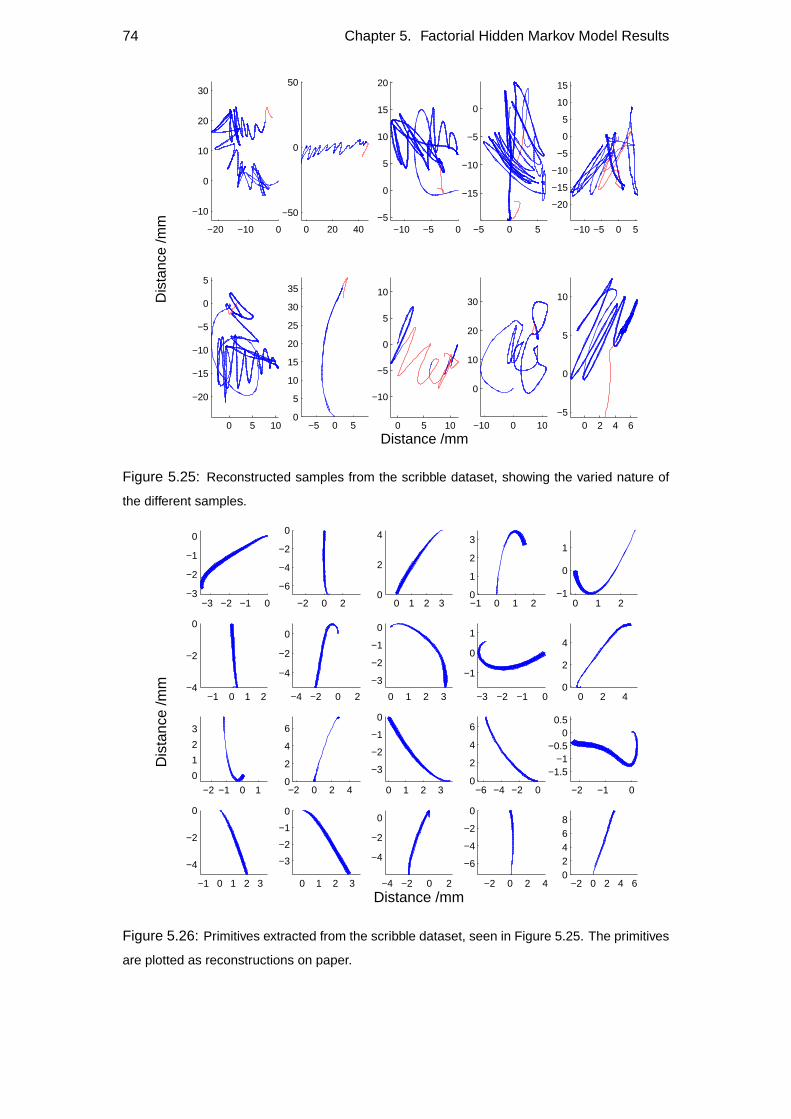
74 Chapter 5. Factorial Hidden Markov Model Results
−20 −10 0
−10
0
10
20
30
Dis
tanc
e /m
m 0 20 40
−50
0
50
−10 −5 0−5
0
5
10
15
20
−5 0 5
−15
−10
−5
0
−10 −5 0 5
−20
−15
−10
−5
0
5
10
15
0 5 10
−20
−15
−10
−5
0
5
−5 0 50
5
10
15
20
25
30
35
0 5 10
−10
−5
0
5
10
Distance /mm−10 0 10
0
10
20
30
0 2 4 6−5
0
5
10
Figure 5.25: Reconstructed samples from the scribble dataset, showing the varied nature of
the different samples.
−3 −2 −1 0−3
−2
−1
0
−2 0 2
−6
−4
−2
0
0 1 2 30
2
4
−1 0 1 20
1
2
3
0 1 2−1
0
1
−1 0 1 2−4
−2
0
Dis
tanc
e /m
m
−4 −2 0 2
−4
−2
0
0 1 2 3
−3
−2
−1
0
−3 −2 −1 0
−1
0
1
0 2 40
2
4
−2 −1 0 1
0
1
2
3
−2 0 2 40
2
4
6
0 1 2 3
−3
−2
−1
0
−6 −4 −2 00
2
4
6
−2 −1 0
−1.5−1
−0.50
0.5
−1 0 1 2 3
−4
−2
0
0 1 2 3
−3
−2
−1
0
−4 −2 0 2
−4
−2
0
Distance /mm−2 0 2 4
−6
−4
−2
0
−2 0 2 4 602468
Figure 5.26: Primitives extracted from the scribble dataset, seen in Figure 5.25. The primitives
are plotted as reconstructions on paper.
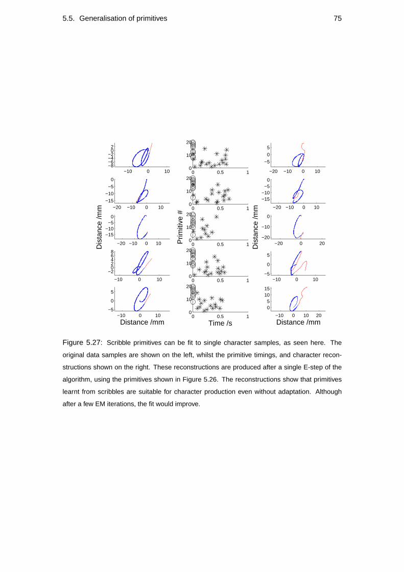
5.5. Generalisation of primitives 75
−10 0 10−8−6−4−2
02
0 0.5 10
10
20
−20 −10 0 10
−5
0
5
−20 −10 0 10−15
−10
−5
0
0 0.5 10
10
20
−20 −10 0 10
−15−10
−50
−20 −10 0 10
−15−10
−50
Dis
tanc
e /m
m
0 0.5 10
10
20
Prim
itive
#
−20 0 20−20
−10
0
Dis
tanc
e /m
m
−10 0 10
−202468
0 0.5 10
10
20
−10 0 10−5
0
5
−10 0 10−5
0
5
Distance /mm0 0.5 1
0
10
20
Time /s−10 0 10 20
05
1015
Distance /mm
Figure 5.27: Scribble primitives can be fit to single character samples, as seen here. The
original data samples are shown on the left, whilst the primitive timings, and character recon-
structions shown on the right. These reconstructions are produced after a single E-step of the
algorithm, using the primitives shown in Figure 5.26. The reconstructions show that primitives
learnt from scribbles are suitable for character production even without adaptation. Although
after a few EM iterations, the fit would improve.
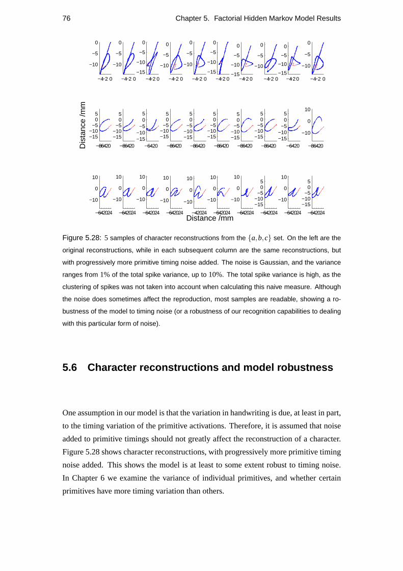
76 Chapter 5. Factorial Hidden Markov Model Results
−4−2 0
−10
−5
0
−4−2 0
−10
−5
0
−4−2 0−15
−10
−5
0
−4−2 0
−10
−5
0
−4−2 0
−10
−5
0
−4−2 0−15
−10
−5
0
−4−2 0−15
−10
−5
0
−4−2 0
−10
−5
0
−4−20−15
−10
−5
0
−4−2 0
−10
−5
0
−8−6−4−20
−15−10
−505
Dis
tanc
e /m
m
−8−6−4−20
−15−10
−505
−6−4−20−15−10
−505
−8−6−4−20
−15−10
−505
−8−6−4−20
−15−10
−505
−8−6−4−20
−15−10
−505
−8−6−4−20
−15−10
−505
−8−6−4−20
−15−10
−505
−6−4−20−15−10
−505
−8−6−4−20
−10
0
10
−6−4−2024
−10
0
10
−6−4−2024
−10
0
10
−6−4−2024
−10
0
10
−6−4−2024
−10
0
10
−4−2024
−10
0
10
Distance /mm−6−4−2024
−10
0
10
−6−4−2024
−10
0
10
−6−4−2024
−15−10
−505
−6−4−2024
−10
0
10
−6−4−2024
−15−10
−505
Figure 5.28: 5 samples of character reconstructions from the {a,b,c} set. On the left are the
original reconstructions, while in each subsequent column are the same reconstructions, but
with progressively more primitive timing noise added. The noise is Gaussian, and the variance
ranges from 1% of the total spike variance, up to 10%. The total spike variance is high, as the
clustering of spikes was not taken into account when calculating this naive measure. Although
the noise does sometimes affect the reproduction, most samples are readable, showing a ro-
bustness of the model to timing noise (or a robustness of our recognition capabilities to dealing
with this particular form of noise).
5.6 Character reconstructions and model robustness
One assumption in our model is that the variation in handwriting is due, at least in part,
to the timing variation of the primitive activations. Therefore, it is assumed that noise
added to primitive timings should not greatly affect the reconstruction of a character.
Figure 5.28 shows character reconstructions, with progressively more primitive timing
noise added. This shows the model is at least to some extent robust to timing noise.
In Chapter 6 we examine the variance of individual primitives, and whether certain
primitives have more timing variation than others.
5.7. Spike timing 77
5.7 Spike timing
The primitives extracted using the model described in Chapter 4 can reconstruct the
dataset, given the appropriate timing information, as demonstrated throughout this
chapter. The process of character reconstruction produces a set of primitive onset
timings or spikes. These spikes are approximations to the full posterior distribution
over the hidden states. Ignoring any self transitions in the hidden states, if allowed, the
spikes are derived from a Viterbi alignment of the hidden states, given a set of prim-
itives. The posterior distribution is referred to asQ(S), so let the Viterbi alignment
of this beQMAP(S). Therefore the spikes that correspond to the onset of primitives are
taken fromQMAP(Smt = 1), where the first non-rest state of the primitives is indexed as
1. Samples of the spike timing data produced can be seen in Figure 5.27 in the central
column.
5.7.1 Generative sampling
So far the model has been used as a framework to extract likely primitives given a
particular dataset, however, as the model is a generative one, it can also be used to
produce data samples. In this case, the hidden states are sampled from the prior dis-
tribution, which is dependent only upon the previous time step, as it is a first order
Markov model. These samples have the form of scribbles, capturing only an aspect of
the character the model was trained upon, as seen in Figure 5.29.
The generative behaviour of the model gives a good impression of what the type
of prior distribution the model captures. In this case, the model is capturing a prior
over pen movements which look locally coherent, and this prior is perhaps suitable for
representing scribbling behaviour. For a character, the local coherence of the primitives
is not enough however, and therefore to make a generative model of characters we must
have a model of the timing of the primitives. This is addressed in Chapter 6.
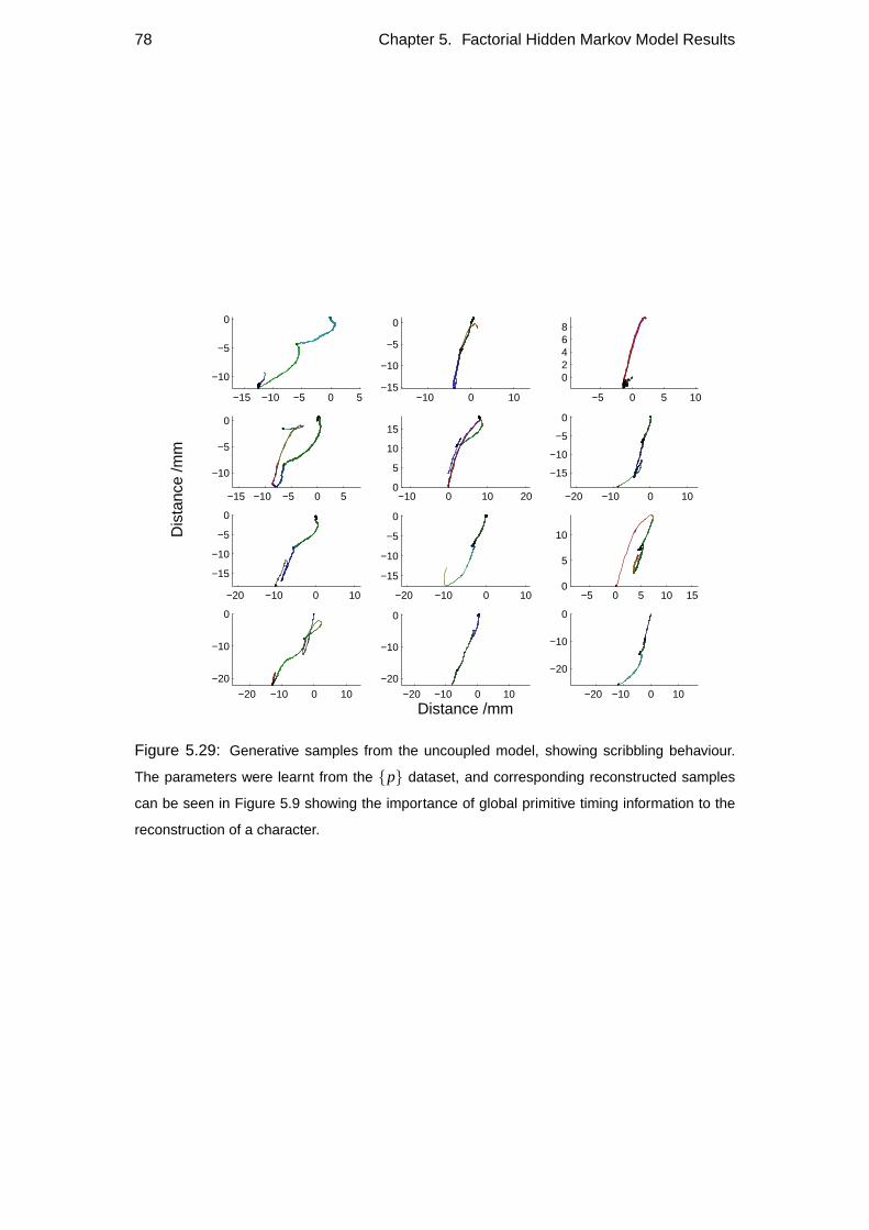
78 Chapter 5. Factorial Hidden Markov Model Results
−15 −10 −5 0 5
−10
−5
0
−10 0 10−15
−10
−5
0
−5 0 5 10
02468
−15 −10 −5 0 5
−10
−5
0
−10 0 10 200
5
10
15
−20 −10 0 10
−15
−10
−5
0
−20 −10 0 10
−15
−10
−5
0
Dis
tanc
e /m
m
−20 −10 0 10
−15
−10
−5
0
−5 0 5 10 150
5
10
−20 −10 0 10
−20
−10
0
−20 −10 0 10
−20
−10
0
Distance /mm−20 −10 0 10
−20
−10
0
Figure 5.29: Generative samples from the uncoupled model, showing scribbling behaviour.
The parameters were learnt from the {p} dataset, and corresponding reconstructed samples
can be seen in Figure 5.9 showing the importance of global primitive timing information to the
reconstruction of a character.
Chapter 6
Timing Model
Chapters 4 and 5 have dealt with the low level model, which provides a prior over what
the pen can do, with short term time dependencies. For producing a generative output
that resembles a human controlling a pen, but not actually writing a coherent charac-
ter, the low level model is suitable. To extend this model so that a generative model of
character production is possible, we need to examine the timing of the primitives, and
generalise over different samples of the same character. This chapter focusses on the
primitive activation, or spike timing data that arises from the hidden state representa-
tion in the low level model. Some areas explored in this chapter have been published
in (Williams et al., 2007).
6.1 Primitive-onset representation of the data
In Chapter 5, the data being modelled was the first differential of the pen tip position,
and pen tip pressure. Sampled trajectory information of this kind is a very inefficient
way of representing the character being drawn. If the pen trajectory arises directly from
some inherent set of motor programs, or motor primitives, as suggested in Chapter 2,
then a more efficient form of representation would take into account these primitives.
If the output is built upon a fixed set of primitives, as described in Chapter 3, then the
data can be transformed into the space of primitive activation timings, as described in
Section 5.7.
To illustrate this transformation, some reconstructed character samples can be seen
in Figure 6.1, along with the primitive activation times for each sample, represented
in the form of spike timings. These spikes can be pooled across all character samples,
and the scatter plot of these spikes can be seen in Figure 6.2, showing the occurrence
79
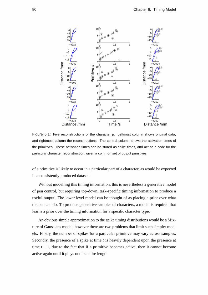
80 Chapter 6. Timing Model
−4−202
−15−10
−50
0 0.5 10
5
10
−4−202
−15−10
−50 ←1←2
←3←3
←4
←5
←6←6←7
←8←9
−4−202
−15−10
−50
0 0.5 10
5
10
−4−2024
−15−10
−50 ←1
←1←2←3
←4←5
←6←6←7←8←9
−4−202−15
−10
−5
0
Dis
tanc
e /m
m
0 0.5 10
5
10
Prim
itive
#
−4−202
−15−10
−50 ←1←2←3
←3
←4
←5
←6←6←7
←8←9
Dis
tanc
e /m
m
−4−202
−15−10
−50
0 0.5 10
5
10
−4−202
−15−10
−50 ←1←2
←3←3
←4
←5
←6←6←7
←8←9
−4−202−15
−10
−5
0
Distance /mm0 0.5 1
0
5
10
Time /s−4−202
−15−10
−5
0 ←1←2←3←3
←4←5
←6←6
←6
←7←8
←9
Distance /mm
Figure 6.1: Five reconstructions of the character p. Leftmost column shows original data,
and rightmost column the reconstructions. The central column shows the activation times of
the primitives. These activation times can be stored as spike times, and act as a code for the
particular character reconstruction, given a common set of output primitives.
of a primitive is likely to occur in a particular part of a character, as would be expected
in a consistently produced dataset.
Without modelling this timing information, this is nevertheless a generative model
of pen control, but requiring top-down, task-specific timing information to produce a
useful output. The lower level model can be thought of as placing a prior over what
the pen can do. To produce generative samples of characters, a model is required that
learns a prior over the timing information for a specific character type.
An obvious simple approximation to the spike timing distributions would be a Mix-
ture of Gaussians model, however there are two problems that limit such simpler mod-
els. Firstly, the number of spikes for a particular primitive may vary across samples.
Secondly, the presence of a spike at timet is heavily dependent upon the presence at
time t − 1, due to the fact that if a primitive becomes active, then it cannot become
active again until it plays out its entire length.
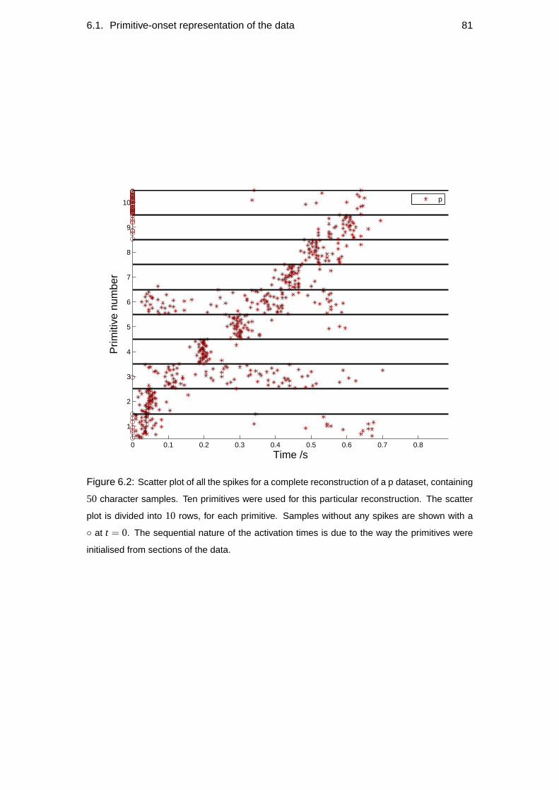
6.1. Primitive-onset representation of the data 81
0 0.1 0.2 0.3 0.4 0.5 0.6 0.7 0.8
1
2
3
4
5
6
7
8
9
10
Time /s
Prim
itive
num
ber
p
Figure 6.2: Scatter plot of all the spikes for a complete reconstruction of a p dataset, containing
50 character samples. Ten primitives were used for this particular reconstruction. The scatter
plot is divided into 10 rows, for each primitive. Samples without any spikes are shown with a
◦ at t = 0. The sequential nature of the activation times is due to the way the primitives were
initialised from sections of the data.
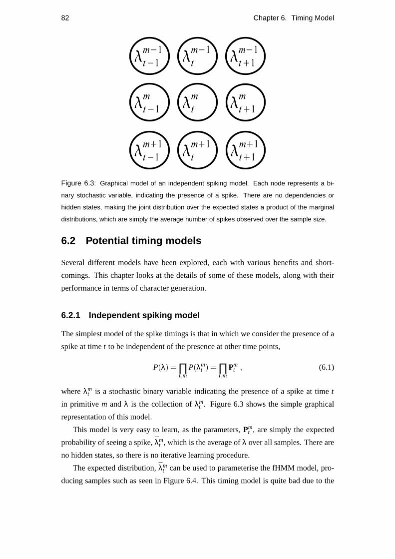
82 Chapter 6. Timing Model
Figure 6.3: Graphical model of an independent spiking model. Each node represents a bi-
nary stochastic variable, indicating the presence of a spike. There are no dependencies or
hidden states, making the joint distribution over the expected states a product of the marginal
distributions, which are simply the average number of spikes observed over the sample size.
6.2 Potential timing models
Several different models have been explored, each with various benefits and short-
comings. This chapter looks at the details of some of these models, along with their
performance in terms of character generation.
6.2.1 Independent spiking model
The simplest model of the spike timings is that in which we consider the presence of a
spike at timet to be independent of the presence at other time points,
P(λ) = ∏t,m
P(λmt ) = ∏
t,mPm
t , (6.1)
whereλmt is a stochastic binary variable indicating the presence of a spike at timet
in primitive m andλ is the collection ofλmt . Figure 6.3 shows the simple graphical
representation of this model.
This model is very easy to learn, as the parameters,Pmt , are simply the expected
probability of seeing a spike,λmt , which is the average ofλ over all samples. There are
no hidden states, so there is no iterative learning procedure.
The expected distribution,λmt can be used to parameterise the fHMM model, pro-
ducing samples such as seen in Figure 6.4. This timing model is quite bad due to the
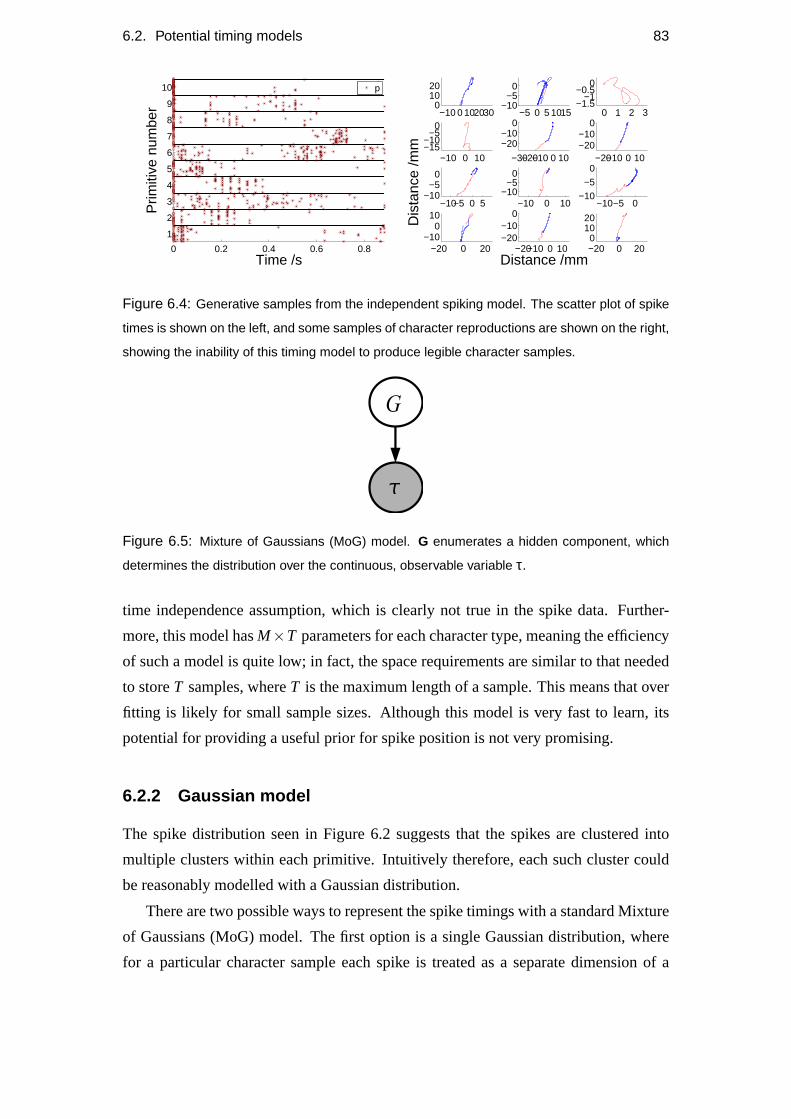
6.2. Potential timing models 83
0 0.2 0.4 0.6 0.8
1
2
3
4
5
6
7
8
9
10
Time /s
Prim
itive
num
ber
p
−10 0 1020300
1020
−5 0 5 1015−10
−50
0 1 2 3−1.5
−1−0.5
0
−10 0 10−15−10
−50
−30−20−10 0 10
−20−10
0
−20−10 0 10−20−10
0
−10−5 0 5−10
−50
Dis
tanc
e /m
m
−10 0 10−10
−50
−10−5 0−10
−50
−20 0 20−10
010
−20−10 0 10−20−10
0
Distance /mm−20 0 200
1020
Figure 6.4: Generative samples from the independent spiking model. The scatter plot of spike
times is shown on the left, and some samples of character reproductions are shown on the right,
showing the inability of this timing model to produce legible character samples.
Figure 6.5: Mixture of Gaussians (MoG) model. G enumerates a hidden component, which
determines the distribution over the continuous, observable variable τ.
time independence assumption, which is clearly not true in the spike data. Further-
more, this model hasM×T parameters for each character type, meaning the efficiency
of such a model is quite low; in fact, the space requirements are similar to that needed
to storeT samples, whereT is the maximum length of a sample. This means that over
fitting is likely for small sample sizes. Although this model is very fast to learn, its
potential for providing a useful prior for spike position is not very promising.
6.2.2 Gaussian model
The spike distribution seen in Figure 6.2 suggests that the spikes are clustered into
multiple clusters within each primitive. Intuitively therefore, each such cluster could
be reasonably modelled with a Gaussian distribution.
There are two possible ways to represent the spike timings with a standard Mixture
of Gaussians (MoG) model. The first option is a single Gaussian distribution, where
for a particular character sample each spike is treated as a separate dimension of a
84 Chapter 6. Timing Model
continuous multivariate Gaussian distribution. The problem with this model is that
the number of spikes per character sample is inconsistent, thereby altering the dimen-
sionality of the Gaussian distribution, and forcing an approximation such as several
Gaussians of different dimensions. Alternatively, the spikes can be pooled, and treated
as independent samples, from a one-dimensional mixture of Gaussians. The second
option will be examined here.
Using this model, the original separate samples must be pooled, and a single sam-
ple, for the purposes of learning the model, be considered to be a single spike. Figure
6.5 shows a MoG model, consisting ofK components,
G ∈ {1, ...,K}
τ ∈R , (6.2)
therefore, the marginal probability density over the output,P(τ), is defined by a weighted
sum of these components,
P(τ) =K
∑k
P(G = k)P(τ |G = k) , (6.3)
where each component is a discrete normal distribution,
P(τ |G = k) = N (µµµk,σ2k) . (6.4)
The parametersµµµ, σ2 and the prior distribution over the components,P(G), are learnt
using a standard EM procedure.
Generatively, as there is no distribution over the number of spikes per sample in-
cluded in this model, the easiest way to sample spikes, and disallow multiple spikes
from the same component is to sample from each component in turn, with the presence
of a spike from componentk equal toP(G = k). If a spike is present from componentk,
this component parameterises the output distributionP(τ |k), being a single Gaussian,
which can then be sampled from, producing a spike time. This is repeatedK times.
This approximation relies on the probability of presence of a particular component be-
ing the same in any one sample as it is across the whole dataset, and that there can
be no dependence between components. Samples of characters generated in such a
manner can be seen in Figure 6.6, with the same dataset containing a single character,
p is shown, along with another dataset containing 3 characters,{a,b,c}. The genera-
tive samples for the dataset with a single character are much better than those from the
mixed dataset, as the primitives used in the mixed dataset need to be shared between
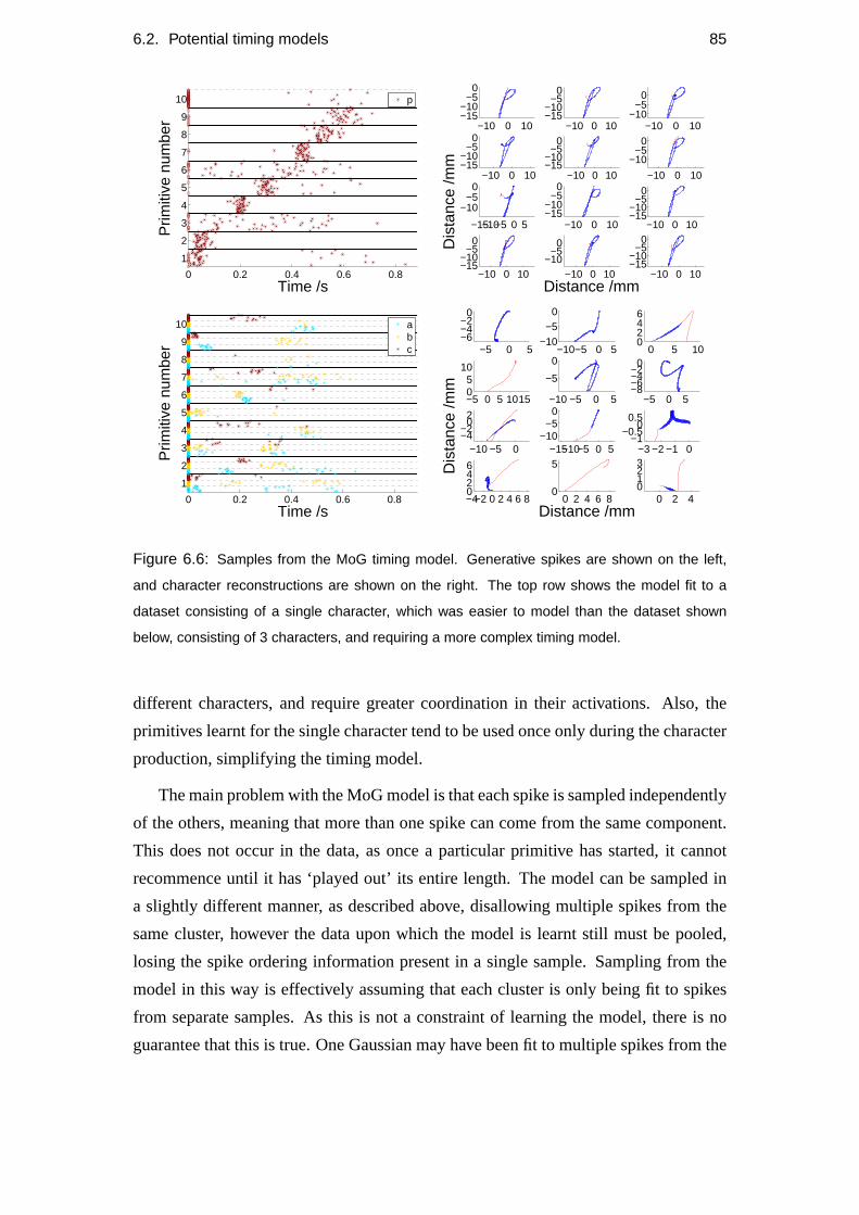
6.2. Potential timing models 85
0 0.2 0.4 0.6 0.8
1
2
3
4
5
6
7
8
9
10
Time /s
Prim
itive
num
ber
p
−10 0 10−15−10
−50
−10 0 10−15−10
−50
−10 0 10−10
−50
−10 0 10−15−10
−50
−10 0 10−15−10
−50
−10 0 10
−10−5
0
−15−10−5 0 5
−10−5
0
Dis
tanc
e /m
m
−10 0 10−15−10
−50
−10 0 10−15−10
−50
−10 0 10−15−10
−50
−10 0 10−10
−50
Distance /mm−10 0 10
−15−10
−50
0 0.2 0.4 0.6 0.8
1
2
3
4
5
6
7
8
9
10
Time /s
Prim
itive
num
ber
abc −5 0 5
−6−4−2
0
−10−5 0 5−10
−50
0 5 100246
−5 0 5 101505
10
−10 −5 0 5
−5
0
−5 0 5−8−6−4−2
0
−10 −5 0−4−2
02
Dis
tanc
e /m
m−15−10−5 0 5
−10−5
0
−3 −2 −1 0−1
−0.50
0.5
−4−2 0 2 4 6 80246
0 2 4 6 80
5
Distance /mm0 2 4
0123
Figure 6.6: Samples from the MoG timing model. Generative spikes are shown on the left,
and character reconstructions are shown on the right. The top row shows the model fit to a
dataset consisting of a single character, which was easier to model than the dataset shown
below, consisting of 3 characters, and requiring a more complex timing model.
different characters, and require greater coordination in their activations. Also, the
primitives learnt for the single character tend to be used once only during the character
production, simplifying the timing model.
The main problem with the MoG model is that each spike is sampled independently
of the others, meaning that more than one spike can come from the same component.
This does not occur in the data, as once a particular primitive has started, it cannot
recommence until it has ‘played out’ its entire length. The model can be sampled in
a slightly different manner, as described above, disallowing multiple spikes from the
same cluster, however the data upon which the model is learnt still must be pooled,
losing the spike ordering information present in a single sample. Sampling from the
model in this way is effectively assuming that each cluster is only being fit to spikes
from separate samples. As this is not a constraint of learning the model, there is no
guarantee that this is true. One Gaussian may have been fit to multiple spikes from the
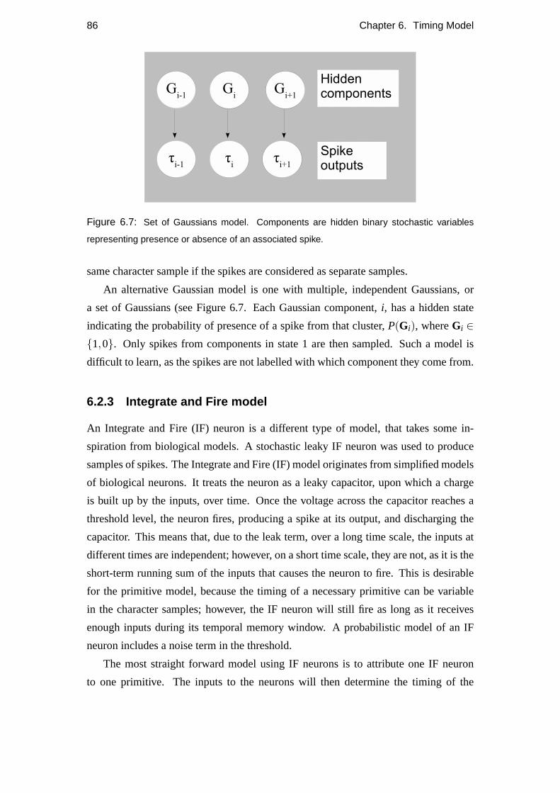
86 Chapter 6. Timing Model
Figure 6.7: Set of Gaussians model. Components are hidden binary stochastic variables
representing presence or absence of an associated spike.
same character sample if the spikes are considered as separate samples.
An alternative Gaussian model is one with multiple, independent Gaussians, or
a set of Gaussians (see Figure 6.7. Each Gaussian component,i, has a hidden state
indicating the probability of presence of a spike from that cluster,P(Gi), whereGi ∈{1,0}. Only spikes from components in state 1 are then sampled. Such a model is
difficult to learn, as the spikes are not labelled with which component they come from.
6.2.3 Integrate and Fire model
An Integrate and Fire (IF) neuron is a different type of model, that takes some in-
spiration from biological models. A stochastic leaky IF neuron was used to produce
samples of spikes. The Integrate and Fire (IF) model originates from simplified models
of biological neurons. It treats the neuron as a leaky capacitor, upon which a charge
is built up by the inputs, over time. Once the voltage across the capacitor reaches a
threshold level, the neuron fires, producing a spike at its output, and discharging the
capacitor. This means that, due to the leak term, over a long time scale, the inputs at
different times are independent; however, on a short time scale, they are not, as it is the
short-term running sum of the inputs that causes the neuron to fire. This is desirable
for the primitive model, because the timing of a necessary primitive can be variable
in the character samples; however, the IF neuron will still fire as long as it receives
enough inputs during its temporal memory window. A probabilistic model of an IF
neuron includes a noise term in the threshold.
The most straight forward model using IF neurons is to attribute one IF neuron
to one primitive. The inputs to the neurons will then determine the timing of the
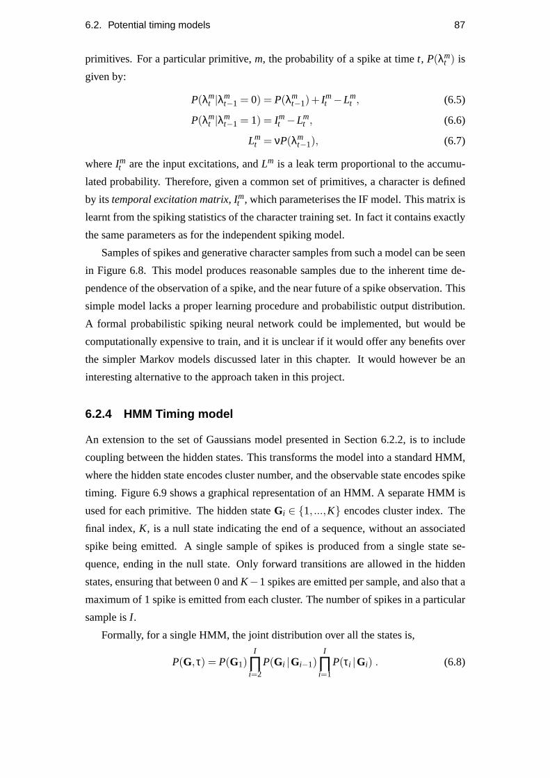
6.2. Potential timing models 87
primitives. For a particular primitive,m, the probability of a spike at timet, P(λmt ) is
given by:
P(λmt |λm
t−1 = 0) = P(λmt−1)+ Im
t −Lmt , (6.5)
P(λmt |λm
t−1 = 1) = Imt −Lm
t , (6.6)
Lmt = νP(λm
t−1), (6.7)
whereImt are the input excitations, andLm is a leak term proportional to the accumu-
lated probability. Therefore, given a common set of primitives, a character is defined
by its temporal excitation matrix, Imt , which parameterises the IF model. This matrix is
learnt from the spiking statistics of the character training set. In fact it contains exactly
the same parameters as for the independent spiking model.
Samples of spikes and generative character samples from such a model can be seen
in Figure 6.8. This model produces reasonable samples due to the inherent time de-
pendence of the observation of a spike, and the near future of a spike observation. This
simple model lacks a proper learning procedure and probabilistic output distribution.
A formal probabilistic spiking neural network could be implemented, but would be
computationally expensive to train, and it is unclear if it would offer any benefits over
the simpler Markov models discussed later in this chapter. It would however be an
interesting alternative to the approach taken in this project.
6.2.4 HMM Timing model
An extension to the set of Gaussians model presented in Section 6.2.2, is to include
coupling between the hidden states. This transforms the model into a standard HMM,
where the hidden state encodes cluster number, and the observable state encodes spike
timing. Figure 6.9 shows a graphical representation of an HMM. A separate HMM is
used for each primitive. The hidden stateGi ∈ {1, ...,K} encodes cluster index. The
final index,K, is a null state indicating the end of a sequence, without an associated
spike being emitted. A single sample of spikes is produced from a single state se-
quence, ending in the null state. Only forward transitions are allowed in the hidden
states, ensuring that between 0 andK−1 spikes are emitted per sample, and also that a
maximum of 1 spike is emitted from each cluster. The number of spikes in a particular
sample isI .
Formally, for a single HMM, the joint distribution over all the states is,
P(G,τ) = P(G1)I
∏i=2
P(Gi |Gi−1)I
∏i=1
P(τi |Gi) . (6.8)
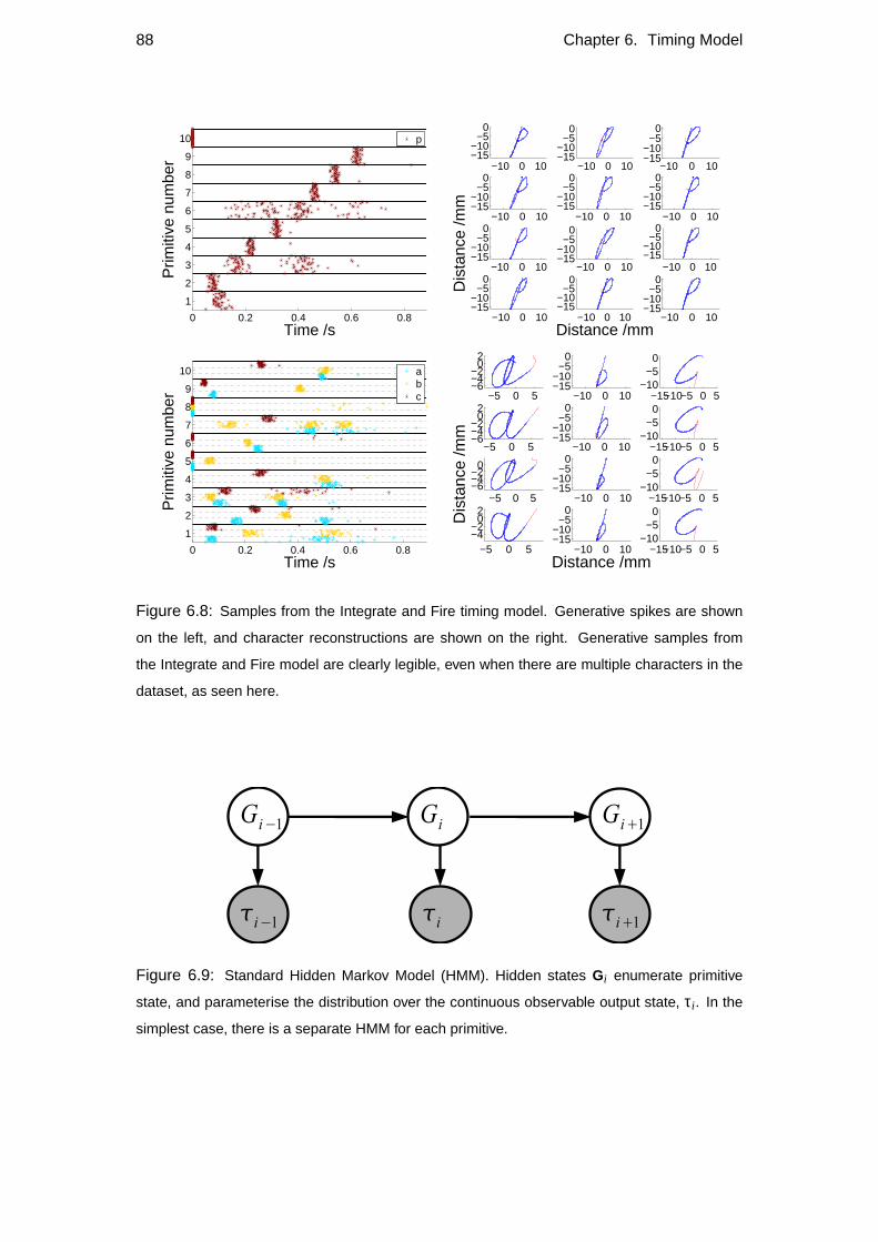
88 Chapter 6. Timing Model
0 0.2 0.4 0.6 0.8
1
2
3
4
5
6
7
8
9
10
Time /s
Prim
itive
num
ber
p
−10 0 10−15−10
−50
−10 0 10−15−10
−50
−10 0 10−15−10
−50
−10 0 10−15−10
−50
−10 0 10−15−10
−50
−10 0 10−15−10
−50
−10 0 10−15−10
−50
Dis
tanc
e /m
m
−10 0 10−15−10
−50
−10 0 10−15−10
−50
−10 0 10−15−10
−50
−10 0 10−15−10
−50
Distance /mm−10 0 10
−15−10
−50
0 0.2 0.4 0.6 0.8
1
2
3
4
5
6
7
8
9
10
Time /s
Prim
itive
num
ber
abc −5 0 5
−6−4−2
02
−10 0 10−15−10
−50
−15−10−5 0 5−10
−50
−5 0 5−6−4−2
02
−10 0 10−15−10
−50
−15−10−5 0 5−10
−50
−5 0 5−6−4−2
0D
ista
nce
/mm
−10 0 10−15−10
−50
−15−10−5 0 5−10
−50
−5 0 5−4−2
02
−10 0 10−15−10
−50
Distance /mm−15−10−5 0 5
−10−5
0
Figure 6.8: Samples from the Integrate and Fire timing model. Generative spikes are shown
on the left, and character reconstructions are shown on the right. Generative samples from
the Integrate and Fire model are clearly legible, even when there are multiple characters in the
dataset, as seen here.
Figure 6.9: Standard Hidden Markov Model (HMM). Hidden states Gi enumerate primitive
state, and parameterise the distribution over the continuous observable output state, τi . In the
simplest case, there is a separate HMM for each primitive.
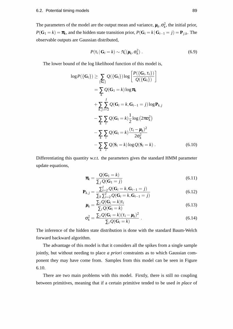
6.2. Potential timing models 89
The parameters of the model are the output mean and variance,µµµk,σ2k, the initial prior,
P(G1 = k) = πππk, and the hidden state transition prior,P(Gi = k|Gi−1 = j) = P j,k. The
observable outputs are Gaussian distributed,
P(τi |Gi = k)∼N (µµµk,σ2k) . (6.9)
The lower bound of the log likelihood function of this model is,
logP({Gi})≥ ∑{Gi}
Q({Gi}) log
[P({Gi ,τi})Q({Gi})
]= ∑
k
Q(G1 = k) logπππk
+∑k, j
I
∑i=2
Q(Gi = k,Gi−1 = j) logPk, j
−∑k
∑i
Q(Gi = k)12
log(2πσ2
k
)−∑
k∑i
Q(Gi = k)(τi−µµµk)
2
2σ2k
−∑k
∑i
Q(Si = k) logQ(Si = k) . (6.10)
Differentiating this quantity w.r.t. the parameters gives the standard HMM parameter
update equations,
πππk =Q(G1 = k)
∑ j Q(G1 = j)(6.11)
Pk, j = ∑Ii=2Q(Gi = k,Gi−1 = j)
∑k ∑Ii=2Q(Gi = k,Gi−1 = j)
(6.12)
µµµk = ∑i Q(Gi = k)τi
∑i Q(Gi = k)(6.13)
σ2k = ∑i Q(Gi = k)(τi−µµµk)
2
∑i Q(Gi = k). (6.14)
The inference of the hidden state distribution is done with the standard Baum-Welch
forward backward algorithm.
The advantage of this model is that it considers all the spikes from a single sample
jointly, but without needing to placea priori constraints as to which Gaussian com-
ponent they may have come from. Samples from this model can be seen in Figure
6.10.
There are two main problems with this model. Firstly, there is still no coupling
between primitives, meaning that if a certain primitive tended to be usedin placeof
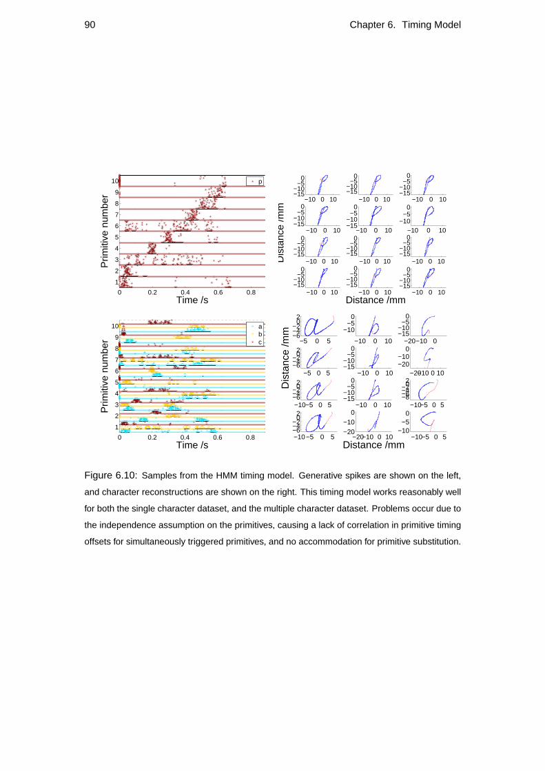
90 Chapter 6. Timing Model
0 0.2 0.4 0.6 0.8
1
2
3
4
5
6
7
8
9
10
Time /s
Prim
itive
num
ber
p
−10 0 10−15−10
−50
−10 0 10−15−10
−50
−10 0 10−15−10
−50
−10 0 10−15−10
−50
Dis
tanc
e /m
m
−10 0 10−15−10
−50
−10 0 10−10
−50
−10 0 10−15−10
−50
−10 0 10−15−10
−50
−10 0 10−15−10
−50
−10 0 10−15−10
−50
−10 0 10−15−10
−50
Distance /mm−10 0 10
−15−10
−50
0 0.2 0.4 0.6 0.8
1
2
3
4
5
6
7
8
9
10
Time /s
Prim
itive
num
ber
abc −5 0 5
−6−4−2
02
−10 0 10
−10−5
0
−20−10 0−15−10
−50
−5 0 5−6−4−20
2
Dis
tanc
e /m
m
−10 0 10−15−10
−50
−20−10 0 10−20−10
0
−10−5 0 5−6−4−20
2
−10 0 10−15−10
−50
−10−5 0 5−8−6−4−20
2
−10−5 0 5−6−4−2
02
−20−10 0 10−20−10
0
Distance /mm−10−5 0 5
−10−5
0
Figure 6.10: Samples from the HMM timing model. Generative spikes are shown on the left,
and character reconstructions are shown on the right. This timing model works reasonably well
for both the single character dataset, and the multiple character dataset. Problems occur due to
the independence assumption on the primitives, causing a lack of correlation in primitive timing
offsets for simultaneously triggered primitives, and no accommodation for primitive substitution.
6.2. Potential timing models 91
another primitive, this anti-correlation in primitive presence would not be captured
by this model. Secondly, the Gaussian outputs are independent, which is necessary
because spikes are not present in all samples from all components, making it impos-
sible to learn a joint Gaussian. This is a problem because there may be spike timing
correlations between spikes from the same primitive, and also between spikes from dif-
ferent primitives. Two extensions to the basic independent HMM timing model were
explored, and are detailed here. One uses a global offset to perform dynamic time
warping, and the other attempts to introduce coupling between the presence or absence
of primitives, by extending the model to a higher level, called character modes.
6.2.4.1 Dynamic time warping
To examine any correlations between spike timings, the offsets of the observed spikes
from the model expectation can be seen in Figure 6.11. Some characters appear to
have correlations between spike offsets in certain areas, suggesting that there should
be some common offset that captures these correlations. It would be difficult to build
such a parameter into the model, but a simple ‘running offset’ can be calculated by
fitting a best fit spline function to the pooled offsets, as in Figure 6.11. By limiting
the spline function to be a polynomial function of limited degree, over fitting can be
controlled. Using such a time warping procedure to estimate the drifting time offset
of each sample, and adjust the spike times accordingly before fitting the timing model
improves the the fit of the model. Figure 6.12 shows the fit of the Gaussian distributions
to spike data before and after time warping of the spikes. In this example, the sum of
the variances of the output distributions was roughly halved due to the time warping
providing a better fit.
The problem with using dynamic time warping is that the length of the characters
tend to reduce, so that the total error of the fit is reduced. Also it further complicates
the inference procedure by adding a further non-probabilistic part to the model, which
means that the likelihood function is no longer valid from one iteration to the next.
The technique is generally unsuitable to be used during inference, but it does provide
a convenient way to reduce variance in the final model before generative samples are
produced, if necessary.
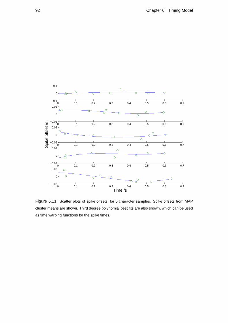
92 Chapter 6. Timing Model
0 0.1 0.2 0.3 0.4 0.5 0.6 0.7−0.1
0
0.1
0 0.1 0.2 0.3 0.4 0.5 0.6 0.7−0.05
0
0.05
0 0.1 0.2 0.3 0.4 0.5 0.6 0.7−0.05
0
0.05
Spi
ke o
ffset
/s
0 0.1 0.2 0.3 0.4 0.5 0.6 0.7−0.02
0
0.02
0 0.1 0.2 0.3 0.4 0.5 0.6 0.7−0.02
0
0.02
Time /s
Figure 6.11: Scatter plots of spike offsets, for 5 character samples. Spike offsets from MAP
cluster means are shown. Third degree polynomial best fits are also shown, which can be used
as time warping functions for the spike times.
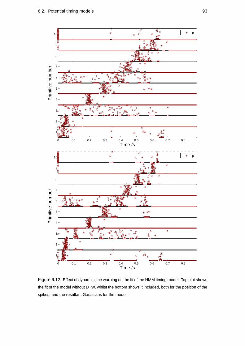
6.2. Potential timing models 93
0 0.1 0.2 0.3 0.4 0.5 0.6 0.7 0.8
1
2
3
4
5
6
7
8
9
10
Time /s
Prim
itive
num
ber
p
0 0.1 0.2 0.3 0.4 0.5 0.6 0.7 0.8
1
2
3
4
5
6
7
8
9
10
Time /s
Prim
itive
num
ber
p
Figure 6.12: Effect of dynamic time warping on the fit of the HMM timing model. Top plot shows
the fit of the model without DTW, whilst the bottom shows it included, both for the position of the
spikes, and the resultant Gaussians for the model.
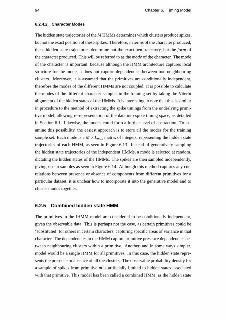
94 Chapter 6. Timing Model
6.2.4.2 Character Modes
The hidden state trajectories of theM HMMs determines which clusters produce spikes,
but not the exact position of these spikes. Therefore, in terms of the character produced,
these hidden state trajectories determine not the exact pen trajectory, but theform of
the character produced. This will be referred to as themodeof the character. The mode
of the character is important, because although the HMM architecture captures local
structure for the mode, it does not capture dependencies between non-neighbouring
clusters. Moreover, it is assumed that the primitives are conditionally independent,
therefore the modes of the different HMMs are not coupled. It is possible to calculate
the modes of the different character samples in the training set by taking the Viterbi
alignment of the hidden states of the HMMs. It is interesting to note that this is similar
in procedure to the method of extracting the spike timings from the underlying primi-
tive model, allowing re-representation of the data into spike timing space, as detailed
in Section 6.1. Likewise, the modes could form a further level of abstraction. To ex-
amine this possibility, the easiest approach is to store all the modes for the training
sample set. Each mode is aM×Lmax matrix of integers, representing the hidden state
trajectories of each HMM, as seen in Figure 6.13. Instead of generatively sampling
the hidden state trajectories of the independent HMMs, a mode is selected at random,
dictating the hidden states of the HMMs. The spikes are then sampled independently,
giving rise to samples as seen in Figure 6.14. Although this method captures any cor-
relations between presence or absence of components from different primitives for a
particular dataset, it is unclear how to incorporate it into the generative model and to
cluster modes together.
6.2.5 Combined hidden state HMM
The primitives in the fHMM model are considered to be conditionally independent,
given the observable data. This is perhaps not the case, as certain primitives could be
‘substituted’ for others in certain characters, capturing specific areas of variance in that
character. The dependencies in the HMM capture primitive presence dependencies be-
tween neighbouring clusters within a primitive. Another, and in some ways simpler,
model would be a single HMM for all primitives. In this case, the hidden state repre-
sents the presence or absence of all the clusters. The observable probability density for
a sample of spikes from primitivem is artificially limited to hidden states associated
with that primitive. This model has been called a combined HMM, as the hidden state
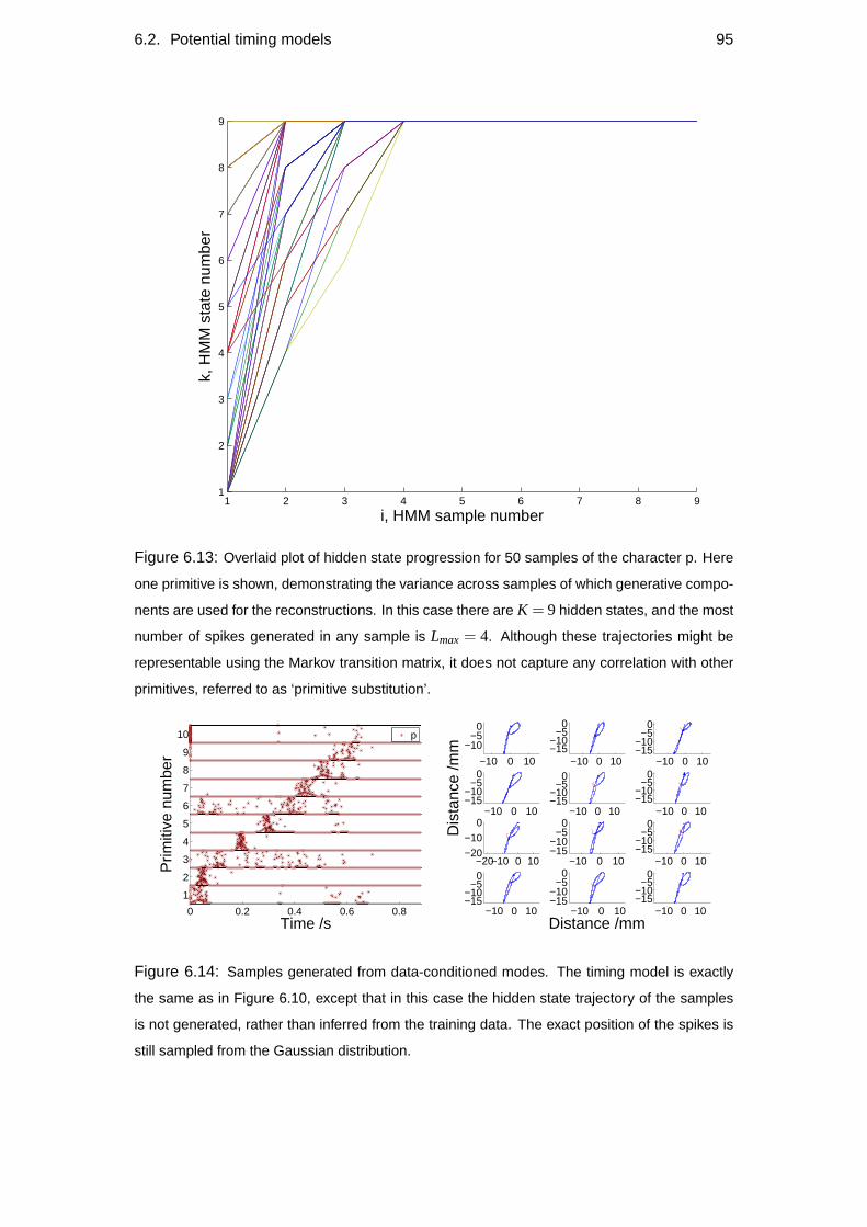
6.2. Potential timing models 95
1 2 3 4 5 6 7 8 91
2
3
4
5
6
7
8
9
i, HMM sample number
k, H
MM
sta
te n
umbe
r
Figure 6.13: Overlaid plot of hidden state progression for 50 samples of the character p. Here
one primitive is shown, demonstrating the variance across samples of which generative compo-
nents are used for the reconstructions. In this case there are K = 9 hidden states, and the most
number of spikes generated in any sample is Lmax = 4. Although these trajectories might be
representable using the Markov transition matrix, it does not capture any correlation with other
primitives, referred to as ‘primitive substitution’.
0 0.2 0.4 0.6 0.8
1
2
3
4
5
6
7
8
9
10
Time /s
Prim
itive
num
ber
p
−10 0 10
−10−5
0
−10 0 10−15−10
−50
−10 0 10−15−10
−50
−10 0 10−15−10
−50
Dis
tanc
e /m
m
−10 0 10−15−10
−50
−10 0 10−15−10
−50
−20−10 0 10−20−10
0
−10 0 10−15−10
−50
−10 0 10−15−10
−50
−10 0 10−15−10
−50
−10 0 10−15−10
−50
Distance /mm−10 0 10
−15−10
−50
Figure 6.14: Samples generated from data-conditioned modes. The timing model is exactly
the same as in Figure 6.10, except that in this case the hidden state trajectory of the samples
is not generated, rather than inferred from the training data. The exact position of the spikes is
still sampled from the Gaussian distribution.
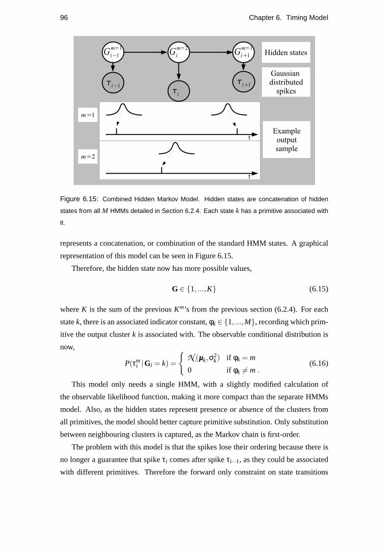
96 Chapter 6. Timing Model
Figure 6.15: Combined Hidden Markov Model. Hidden states are concatenation of hidden
states from all M HMMs detailed in Section 6.2.4. Each state k has a primitive associated with
it.
represents a concatenation, or combination of the standard HMM states. A graphical
representation of this model can be seen in Figure 6.15.
Therefore, the hidden state now has more possible values,
G ∈ {1, ...,K} (6.15)
whereK is the sum of the previousKm’s from the previous section (6.2.4). For each
statek, there is an associated indicator constant,φk∈ {1, ...,M}, recording which prim-
itive the output clusterk is associated with. The observable conditional distribution is
now,
P(τmi |Gi = k) =
{N (µµµk,σ2
k) if φk = m
0 if φk 6= m .(6.16)
This model only needs a single HMM, with a slightly modified calculation of
the observable likelihood function, making it more compact than the separate HMMs
model. Also, as the hidden states represent presence or absence of the clusters from
all primitives, the model should better capture primitive substitution. Only substitution
between neighbouring clusters is captured, as the Markov chain is first-order.
The problem with this model is that the spikes lose their ordering because there is
no longer a guarantee that spikeτi comes after spikeτi−1, as they could be associated
with different primitives. Therefore the forward only constraint on state transitions
6.2. Potential timing models 97
must be relaxed for the model to be learnt, which makes the generative samples incon-
sistent, as a cluster might be activated more than once.
6.2.6 Single combined HMM
A subtly different HMM timing model solves the above problems, by dividing the
parameters of the model into two sets. In Section 6.2.4 a timing model withM separate
HMMs was described, therefore usingM sets of transition parameters (πππk,Pk, j ), and
M sets of output parameters (µµµk,σ2k). In Section 6.2.5, the hidden state was combined,
implying a single set of transition parameters, however the output parameters were still
associated with a particular primitive, limiting the possible transitions between states
in a manner inconsistent with the constraints needed. This can be better understood by
considering that thek’s and thei’s may not come in the same temporal order.
In this final model, called the single combined HMM, there areM different sets
of transition parameters1, but the output parameters are shared for all primitives and
characters. Figure 6.16 shows a graphical representation of this model.
There is no longer a clear definition of the maximum number of components in
the model, as only a subset of the components might be used for any one data sample.
Therefore, to determine the number of components,K, a simple local maxima finding
algorithm is used. Procedurally, all the spike timing data is pooled together, and tallied
into bins, as if for a histogram. These tally counts are Gaussian smoothed, and then
it is a simple matter to find local peaks in this function. An example can be seen in
Figure 6.17. If the number of components inferred is lower than the maximum number
of spikes in a single sample, then the resolution of the Gaussian smoothing function is
increased (σ is decreased) and the method is repeated. Not only does this technique
provide a useful estimate of the maximum number of components necessary to model
the data, but it also provides an estimate of the positions of these components, which
is used to initialise the parameters before performing EM on the HMM.
The original motivation for this model was from experiments in character recogni-
tion, which are described in Chapter 8. The benefit of this model is that each character
type has the same number of components, i.e. has the same size model. This means that
the log likelihood can be compared between character models without a bias towards
one with a larger model size. The likelihood is calculated as if there wereM separate
HMMs, as there areM different transition parameters learnt for each primitive.
1In fact there areM×C transition parameters, whereC is the number of character types in the datasetbeing learnt.
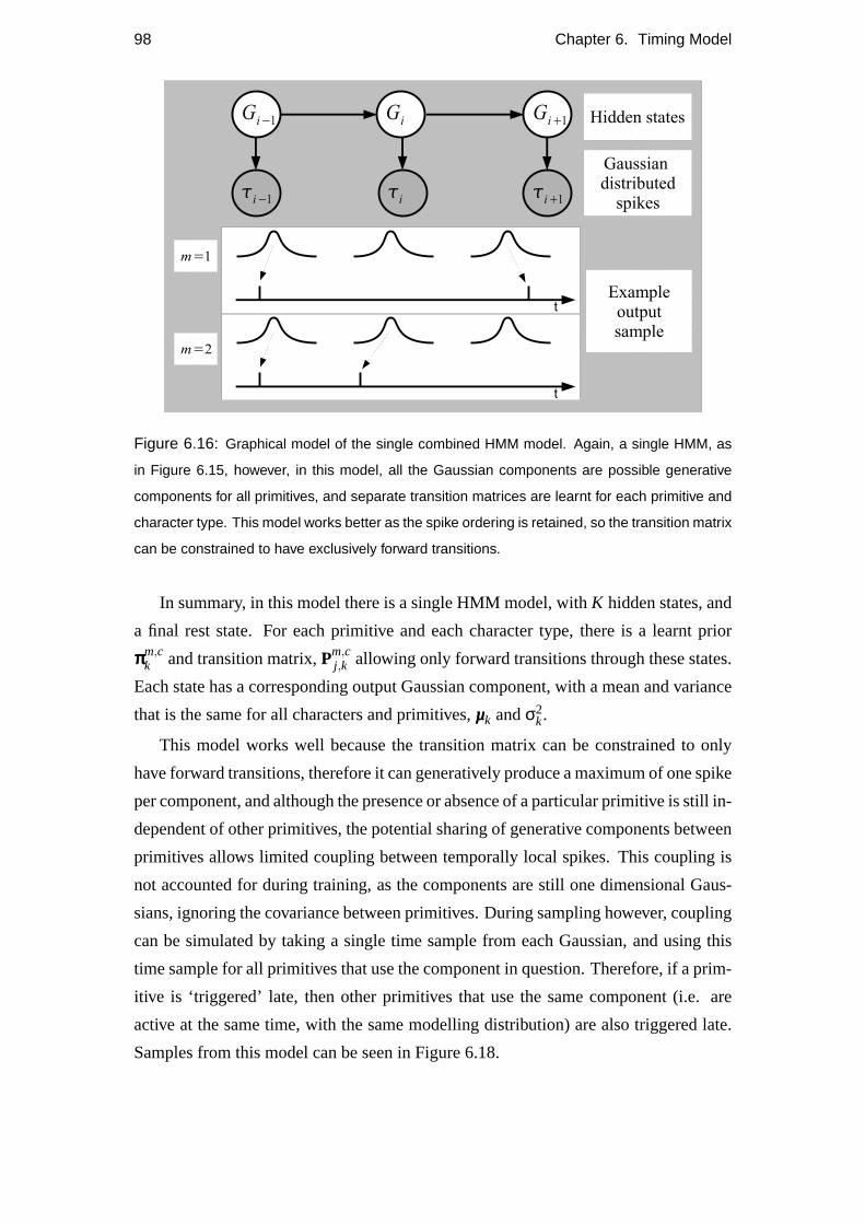
98 Chapter 6. Timing Model
Figure 6.16: Graphical model of the single combined HMM model. Again, a single HMM, as
in Figure 6.15, however, in this model, all the Gaussian components are possible generative
components for all primitives, and separate transition matrices are learnt for each primitive and
character type. This model works better as the spike ordering is retained, so the transition matrix
can be constrained to have exclusively forward transitions.
In summary, in this model there is a single HMM model, withK hidden states, and
a final rest state. For each primitive and each character type, there is a learnt prior
πππm,ck and transition matrix,Pm,c
j,k allowing only forward transitions through these states.
Each state has a corresponding output Gaussian component, with a mean and variance
that is the same for all characters and primitives,µµµk andσ2k.
This model works well because the transition matrix can be constrained to only
have forward transitions, therefore it can generatively produce a maximum of one spike
per component, and although the presence or absence of a particular primitive is still in-
dependent of other primitives, the potential sharing of generative components between
primitives allows limited coupling between temporally local spikes. This coupling is
not accounted for during training, as the components are still one dimensional Gaus-
sians, ignoring the covariance between primitives. During sampling however, coupling
can be simulated by taking a single time sample from each Gaussian, and using this
time sample for all primitives that use the component in question. Therefore, if a prim-
itive is ‘triggered’ late, then other primitives that use the same component (i.e. are
active at the same time, with the same modelling distribution) are also triggered late.
Samples from this model can be seen in Figure 6.18.
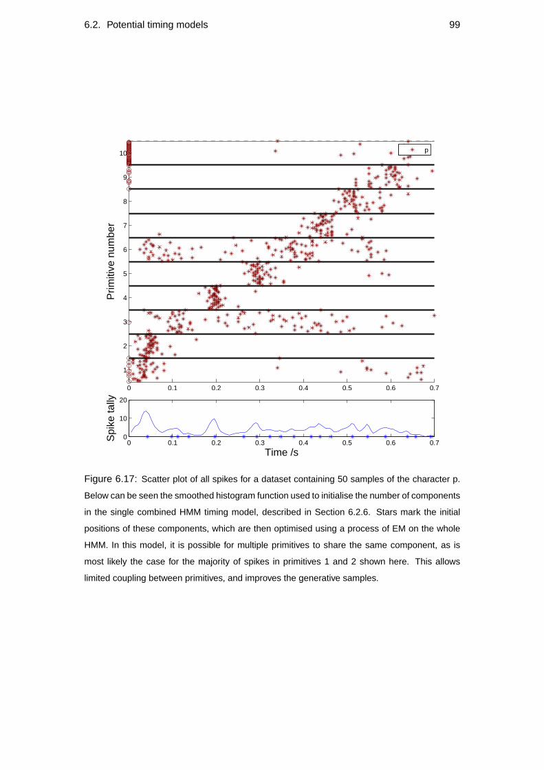
6.2. Potential timing models 99
0 0.1 0.2 0.3 0.4 0.5 0.6 0.7
1
2
3
4
5
6
7
8
9
10
Prim
itive
num
ber
p
0 0.1 0.2 0.3 0.4 0.5 0.6 0.70
10
20
Time /s
Spi
ke ta
lly
Figure 6.17: Scatter plot of all spikes for a dataset containing 50 samples of the character p.
Below can be seen the smoothed histogram function used to initialise the number of components
in the single combined HMM timing model, described in Section 6.2.6. Stars mark the initial
positions of these components, which are then optimised using a process of EM on the whole
HMM. In this model, it is possible for multiple primitives to share the same component, as is
most likely the case for the majority of spikes in primitives 1 and 2 shown here. This allows
limited coupling between primitives, and improves the generative samples.
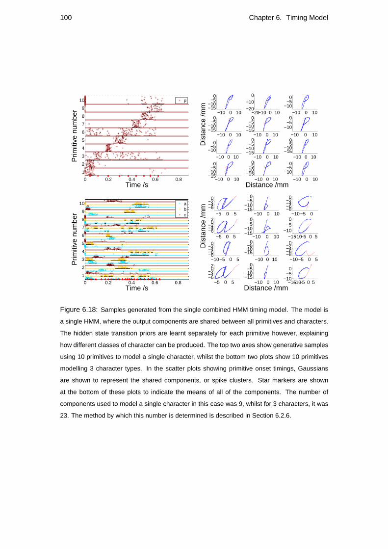
100 Chapter 6. Timing Model
0 0.2 0.4 0.6 0.8
1
2
3
4
5
6
7
8
9
10
Time /s
Prim
itive
num
ber
p
−10 0 10−15−10
−50
−20−10 0 10−20−10
0
−10 0 10−10
−50
−10 0 10−15−10
−50
Dis
tanc
e /m
m
−10 0 10−15−10
−50
−10 0 10
−10−5
0
−10 0 10
−10−5
0
−10 0 10−15−10
−50
−10 0 10−15−10
−50
−10 0 10−15−10
−50
−10 0 10−15−10
−50
Distance /mm−10 0 10
−10−5
0
0 0.2 0.4 0.6 0.8
1
2
3
4
5
6
7
8
9
10
Time /s
Prim
itive
num
ber
abc −5 0 5
−6−4−2
0
−10 0 10−15−10
−50
−10−5 0−8−6−4−2
0
−5 0 5−6−4−2
02
Dis
tanc
e /m
m
−10 0 10−15−10
−50
−15−10−5 0 5−10
−50
−10−5 0 5−8−6−4−2
0
−10 0 10−15−10
−50
−10−5 0 5−8−6−4−2
0
−5 0 5−6−4−2
02
−10 0 10−15−10
−50
Distance /mm−15−10−5 0 5
−10−5
0
Figure 6.18: Samples generated from the single combined HMM timing model. The model is
a single HMM, where the output components are shared between all primitives and characters.
The hidden state transition priors are learnt separately for each primitive however, explaining
how different classes of character can be produced. The top two axes show generative samples
using 10 primitives to model a single character, whilst the bottom two plots show 10 primitives
modelling 3 character types. In the scatter plots showing primitive onset timings, Gaussians
are shown to represent the shared components, or spike clusters. Star markers are shown
at the bottom of these plots to indicate the means of all of the components. The number of
components used to model a single character in this case was 9, whilst for 3 characters, it was
23. The method by which this number is determined is described in Section 6.2.6.
6.3. Generative comparison 101
6.3 Generative comparison
The generative performance of these models can be assessed in several different ways.
Firstly, the most straightforward criteria, is simply the quality of the generative charac-
ter samples produced. However, a simple mean trajectory of character samples would
be a reasonable model by this assessment. The variation of the character samples is
important, as it should capture the variation of the dataset. Furthermore, the models
should be assessed on the size of their parameter spaces.
The dataset containing the characterp and using 10 primitives, as used throughout
this chapter is used here to test the different models for their generative mean and
variance. The original data, as seen in Figure 6.1 has the mean and variance profile seen
in Figure 6.19. Ten primitives were learnt as described in Chapter 4 without the use of a
timing model. A single E-step infers the posterior over the fHMM, giving the primitive
onset times or spikes. This posterior based reconstruction has the mean and variance
profile seen in Figure 6.20, along with the original data, showing a good reconstruction.
It should be noted that these data-conditioned samples are not generative samples.
Generative samples are samples from the prior distributions of the model, as described
below.
Without any timing model present, scribbling behaviour is produced, as seen in
Figure 5.29 in the last chapter. The mean and variance profile from this behaviour can
be seen in Figure 6.21, which as expected, does not match the dataset very well, ex-
cept in average magnitude. The mean and variance profile for the independent spiking
model as described in Section 6.2.1 can be seen in Figure 6.22, showing correspond-
ingly poor profiles for this simple model. The timing model using Gaussian mixtures
to model the spike timings as described in Section 6.2.2 produces better mean and vari-
ance profiles from its generative behaviour, as seen in Figure 6.23. The integrate and
fire model as described in Section 6.2.3 produced very good generative samples, from
a readability point of view; however, the mean and variance profiles seen in Figure
6.24 show that this model does not model the variance of the dataset.
There are three variations of the HMM timing model examined here. Firstly the
separate HMM model, in which there areM independent HMMs modelling theM
primitives, as described in Section 6.2.4. This model produces reasonable character
samples from a single character dataset, and the mean and variance profiles of the
samples are correspondingly good, as seen in Figure 6.25. Using the character modes
as described in Section 6.2.4.2 to condition the hidden states of the separate HMM
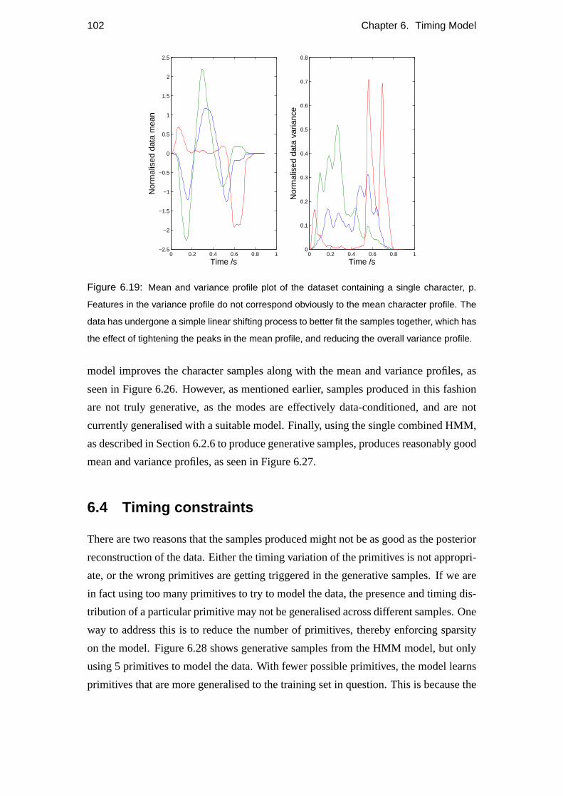
102 Chapter 6. Timing Model
0 0.2 0.4 0.6 0.8 1−2.5
−2
−1.5
−1
−0.5
0
0.5
1
1.5
2
2.5
Time /s
Nor
mal
ised
dat
a m
ean
0 0.2 0.4 0.6 0.8 10
0.1
0.2
0.3
0.4
0.5
0.6
0.7
0.8
Time /s
Nor
mal
ised
dat
a va
rianc
eFigure 6.19: Mean and variance profile plot of the dataset containing a single character, p.
Features in the variance profile do not correspond obviously to the mean character profile. The
data has undergone a simple linear shifting process to better fit the samples together, which has
the effect of tightening the peaks in the mean profile, and reducing the overall variance profile.
model improves the character samples along with the mean and variance profiles, as
seen in Figure 6.26. However, as mentioned earlier, samples produced in this fashion
are not truly generative, as the modes are effectively data-conditioned, and are not
currently generalised with a suitable model. Finally, using the single combined HMM,
as described in Section 6.2.6 to produce generative samples, produces reasonably good
mean and variance profiles, as seen in Figure 6.27.
6.4 Timing constraints
There are two reasons that the samples produced might not be as good as the posterior
reconstruction of the data. Either the timing variation of the primitives is not appropri-
ate, or the wrong primitives are getting triggered in the generative samples. If we are
in fact using too many primitives to try to model the data, the presence and timing dis-
tribution of a particular primitive may not be generalised across different samples. One
way to address this is to reduce the number of primitives, thereby enforcing sparsity
on the model. Figure 6.28 shows generative samples from the HMM model, but only
using 5 primitives to model the data. With fewer possible primitives, the model learns
primitives that are more generalised to the training set in question. This is because the
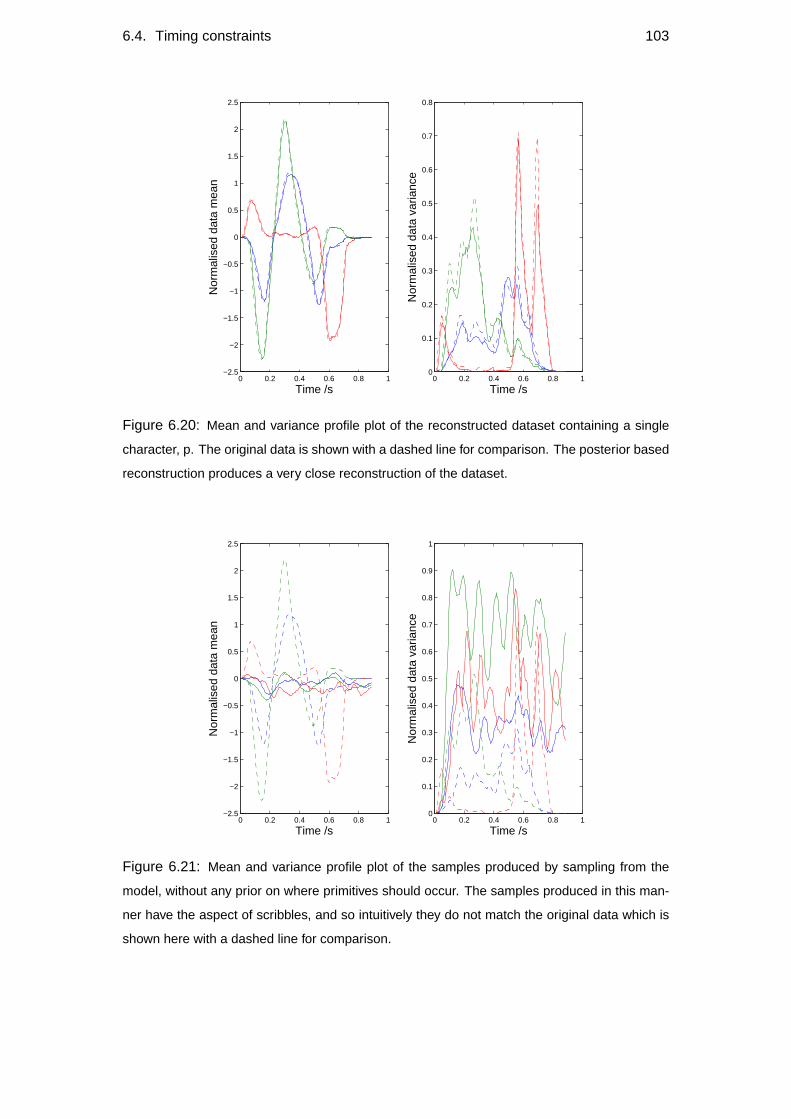
6.4. Timing constraints 103
0 0.2 0.4 0.6 0.8 1−2.5
−2
−1.5
−1
−0.5
0
0.5
1
1.5
2
2.5
Time /s
Nor
mal
ised
dat
a m
ean
0 0.2 0.4 0.6 0.8 10
0.1
0.2
0.3
0.4
0.5
0.6
0.7
0.8
Time /s
Nor
mal
ised
dat
a va
rianc
eFigure 6.20: Mean and variance profile plot of the reconstructed dataset containing a single
character, p. The original data is shown with a dashed line for comparison. The posterior based
reconstruction produces a very close reconstruction of the dataset.
0 0.2 0.4 0.6 0.8 1−2.5
−2
−1.5
−1
−0.5
0
0.5
1
1.5
2
2.5
Time /s
Nor
mal
ised
dat
a m
ean
0 0.2 0.4 0.6 0.8 10
0.1
0.2
0.3
0.4
0.5
0.6
0.7
0.8
0.9
1
Time /s
Nor
mal
ised
dat
a va
rianc
e
Figure 6.21: Mean and variance profile plot of the samples produced by sampling from the
model, without any prior on where primitives should occur. The samples produced in this man-
ner have the aspect of scribbles, and so intuitively they do not match the original data which is
shown here with a dashed line for comparison.
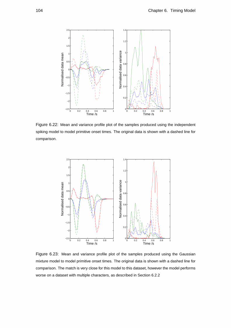
104 Chapter 6. Timing Model
0 0.2 0.4 0.6 0.8 1−2.5
−2
−1.5
−1
−0.5
0
0.5
1
1.5
2
2.5
Time /s
Nor
mal
ised
dat
a m
ean
0 0.2 0.4 0.6 0.8 10
0.2
0.4
0.6
0.8
1
1.2
1.4
Time /s
Nor
mal
ised
dat
a va
rianc
eFigure 6.22: Mean and variance profile plot of the samples produced using the independent
spiking model to model primitive onset times. The original data is shown with a dashed line for
comparison.
0 0.2 0.4 0.6 0.8 1−2.5
−2
−1.5
−1
−0.5
0
0.5
1
1.5
2
2.5
Time /s
Nor
mal
ised
dat
a m
ean
0 0.2 0.4 0.6 0.8 10
0.2
0.4
0.6
0.8
1
1.2
1.4
Time /s
Nor
mal
ised
dat
a va
rianc
e
Figure 6.23: Mean and variance profile plot of the samples produced using the Gaussian
mixture model to model primitive onset times. The original data is shown with a dashed line for
comparison. The match is very close for this model to this dataset, however the model performs
worse on a dataset with multiple characters, as described in Section 6.2.2
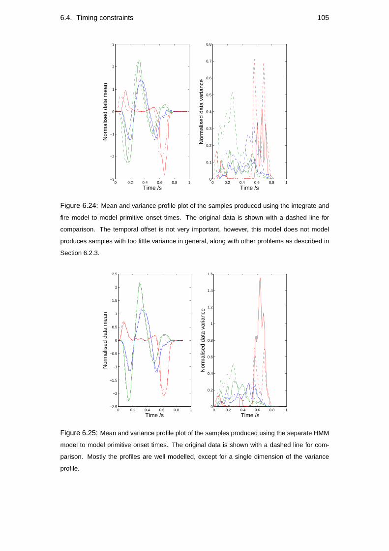
6.4. Timing constraints 105
0 0.2 0.4 0.6 0.8 1−3
−2
−1
0
1
2
3
Time /s
Nor
mal
ised
dat
a m
ean
0 0.2 0.4 0.6 0.8 10
0.1
0.2
0.3
0.4
0.5
0.6
0.7
0.8
Time /s
Nor
mal
ised
dat
a va
rianc
eFigure 6.24: Mean and variance profile plot of the samples produced using the integrate and
fire model to model primitive onset times. The original data is shown with a dashed line for
comparison. The temporal offset is not very important, however, this model does not model
produces samples with too little variance in general, along with other problems as described in
Section 6.2.3.
0 0.2 0.4 0.6 0.8 1−2.5
−2
−1.5
−1
−0.5
0
0.5
1
1.5
2
2.5
Time /s
Nor
mal
ised
dat
a m
ean
0 0.2 0.4 0.6 0.8 10
0.2
0.4
0.6
0.8
1
1.2
1.4
1.6
Time /s
Nor
mal
ised
dat
a va
rianc
e
Figure 6.25: Mean and variance profile plot of the samples produced using the separate HMM
model to model primitive onset times. The original data is shown with a dashed line for com-
parison. Mostly the profiles are well modelled, except for a single dimension of the variance
profile.
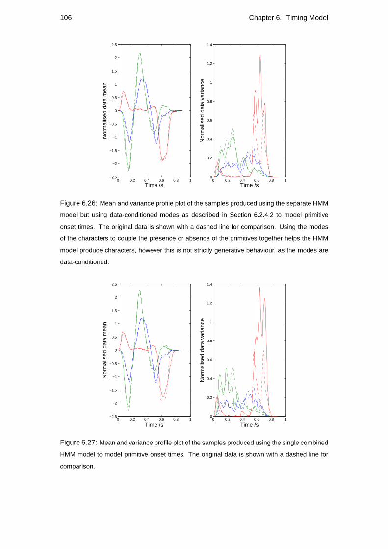
106 Chapter 6. Timing Model
0 0.2 0.4 0.6 0.8 1−2.5
−2
−1.5
−1
−0.5
0
0.5
1
1.5
2
2.5
Time /s
Nor
mal
ised
dat
a m
ean
0 0.2 0.4 0.6 0.8 10
0.2
0.4
0.6
0.8
1
1.2
1.4
Time /s
Nor
mal
ised
dat
a va
rianc
eFigure 6.26: Mean and variance profile plot of the samples produced using the separate HMM
model but using data-conditioned modes as described in Section 6.2.4.2 to model primitive
onset times. The original data is shown with a dashed line for comparison. Using the modes
of the characters to couple the presence or absence of the primitives together helps the HMM
model produce characters, however this is not strictly generative behaviour, as the modes are
data-conditioned.
0 0.2 0.4 0.6 0.8 1−2.5
−2
−1.5
−1
−0.5
0
0.5
1
1.5
2
2.5
Time /s
Nor
mal
ised
dat
a m
ean
0 0.2 0.4 0.6 0.8 10
0.2
0.4
0.6
0.8
1
1.2
1.4
Time /s
Nor
mal
ised
dat
a va
rianc
e
Figure 6.27: Mean and variance profile plot of the samples produced using the single combined
HMM model to model primitive onset times. The original data is shown with a dashed line for
comparison.
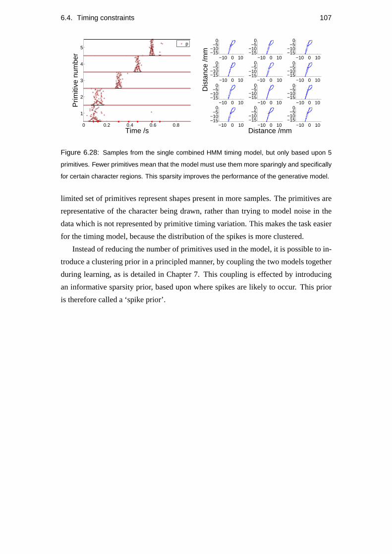
6.4. Timing constraints 107
0 0.2 0.4 0.6 0.8
1
2
3
4
5
Time /s
Prim
itive
num
ber
p
−10 0 10−15−10
−50
−10 0 10−15−10
−50
−10 0 10−15−10
−50
−10 0 10−15−10
−50
Dis
tanc
e /m
m
−10 0 10−15−10
−50
−10 0 10−15−10
−50
−10 0 10−15−10
−50
−10 0 10−15−10
−50
−10 0 10−15−10
−50
−10 0 10−15−10
−50
−10 0 10−15−10
−50
Distance /mm−10 0 10
−15−10
−50
Figure 6.28: Samples from the single combined HMM timing model, but only based upon 5
primitives. Fewer primitives mean that the model must use them more sparingly and specifically
for certain character regions. This sparsity improves the performance of the generative model.
limited set of primitives represent shapes present in more samples. The primitives are
representative of the character being drawn, rather than trying to model noise in the
data which is not represented by primitive timing variation. This makes the task easier
for the timing model, because the distribution of the spikes is more clustered.
Instead of reducing the number of primitives used in the model, it is possible to in-
troduce a clustering prior in a principled manner, by coupling the two models together
during learning, as is detailed in Chapter 7. This coupling is effected by introducing
an informative sparsity prior, based upon where spikes are likely to occur. This prior
is therefore called a ‘spike prior’.

Chapter 7
Coupled Model
In Chapters 4 and 6, two levels of model have been discussed. Firstly, the low level
model was presented, which captures the overlapping primitive segments, and pro-
vides a prior over general pen-movements, as can be seen in Figure 5.29. To provide
a generative model for writing, the next stage is to model the timing of the primitives
and generalise across different samples of the same character. Several different timing
models were discussed in Chapter 6, along with their advantages and shortcomings.
Although the HMM model is a nice solution, producing reasonable generative char-
acter samples, when using many primitives, it has a tendency to over fit the data, as
the primitives are learnt as though the data is meaningless scribble, without timing
dependence upon primitive onset. This means that the primitives can often be fit to in-
appropriate parts of the character for specific character samples, making a generalised
timing model difficult to fit.
A better way to learn the primitives would be to use an informed prior for the prim-
itive onset probabilities. This prior comes from a timing model, which is in turn learnt
from the spike data extracted using the low level fHMM primitive model. This cou-
pling of the models during learning is an iterative process, which can be implemented
during the EM inference of the fHMM.
Due to the compression of the data into the form of spike times, the inference of the
timing model is considerably faster than for the primitive model, therefore there is not
a huge difference in inference time for the coupled model as opposed to the uncoupled
fHMM.
This chapter details the method of coupling of the low level primitive model, and
the higher level timing model. The full coupled model can be learnt in an iterative
variational manner, and is discussed in this chapter, along with the difference that
109
110 Chapter 7. Coupled Model
the coupling makes to the parameters learnt. The coupled model presented here is
published in (Williams et al., 2008).
7.1 Coupling method
The single combined HMM timing model introduced in Section 6.2.6 is adopted to
model the spike data representing the primitive onsets. These spike timings are derived
from the posterior over the hidden states of the primitive model, as discussed in Section
6.1, and provide an intermediate representation of the data. This representation is
much more compact than the observable trajectory data, and allows more compact
higher level models to be introduced that can more easily generalise across different
character samples. To learn the models in a coupled fashion, we firstly look at the
output distribution of the HMM timing model.
The HMM timing model is used to provide a mixture of Gaussians distribution
where the presence or absence of a component is inferred from the data. A graphical
form of the timing model can be seen in Figure 7.1. There is one timing model with
separate transition parameters for each primitive. The timing model is a standard HMM
with one dimensional Gaussian outputs representing the time of an indexed spike. Each
spike, which represents the onset of a primitive, is assumed to come from a specific
generating Gaussian component; however the components do not reliably generate
spikes, as evidenced by the varying number of spikes per character sample.
The data being modelled by the HMM is a set ofI spikes,{τ1,τ2, ...,τI}. The
number of spikes per sample varies, but they are assumed to originate from consistent
generative components, modelled by Gaussian distributions. Each component is as-
sumed to give rise to at most one spike. The component generating a particular spike
is modelled in the hidden state of the model,Gi ∈ {1...K}, whereP(Gi = k) is the
probability that spikei is generated by thekth component. It should be noted thatK is
therefore the maximum value ofI taken over all samples.
The timing model provides a distribution over the timing of an indexed spike
P(τi) =K
∑Gi=1
P(τi |Gi)P(Gi) , (7.1)
whereτi is a continuous variable representing the time of spikei in a sequence ofI
spikes (from a single primitive).Gi ∈ {1..K} is a discrete variable, indicating that
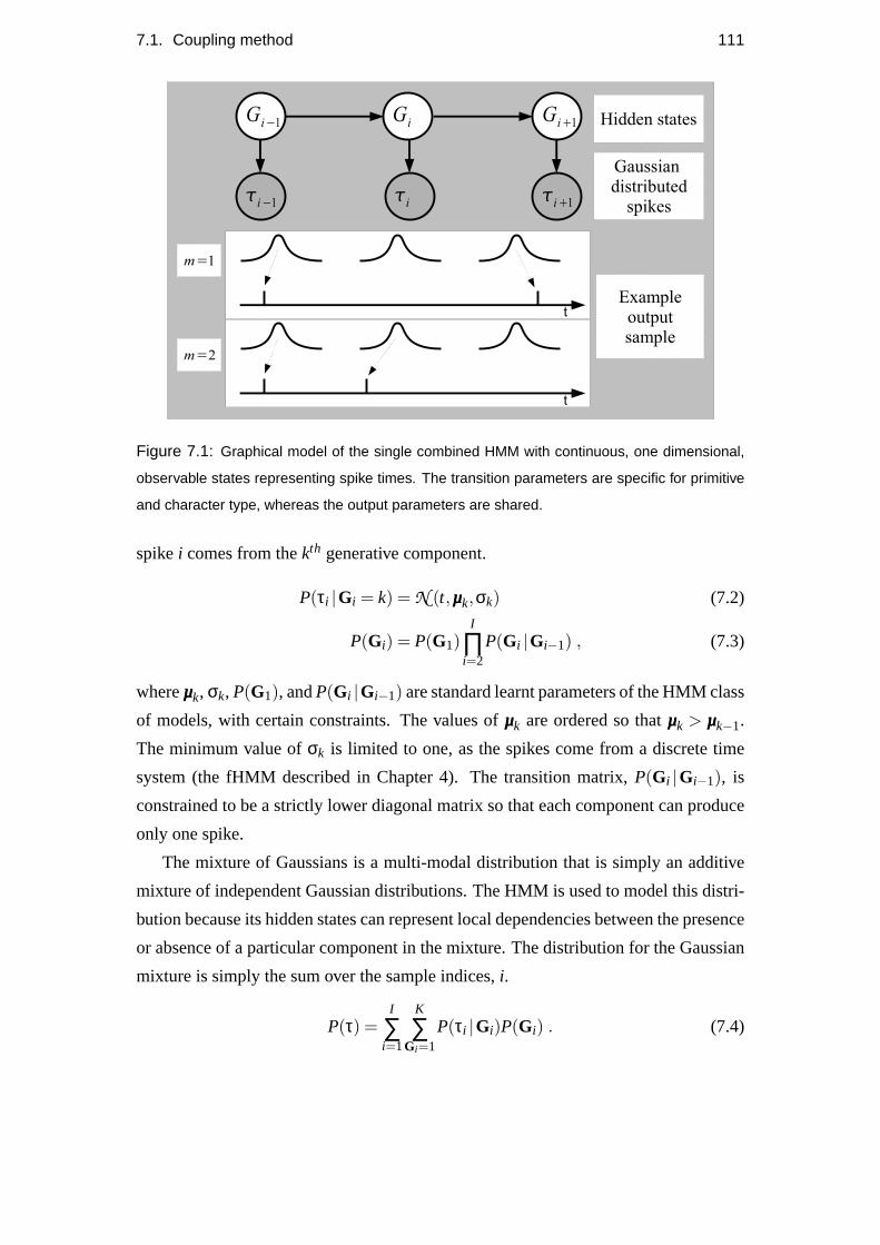
7.1. Coupling method 111
Figure 7.1: Graphical model of the single combined HMM with continuous, one dimensional,
observable states representing spike times. The transition parameters are specific for primitive
and character type, whereas the output parameters are shared.
spikei comes from thekth generative component.
P(τi |Gi = k) = N (t,µµµk,σk) (7.2)
P(Gi) = P(G1)I
∏i=2
P(Gi |Gi−1) , (7.3)
whereµµµk, σk, P(G1), andP(Gi |Gi−1) are standard learnt parameters of the HMM class
of models, with certain constraints. The values ofµµµk are ordered so thatµµµk > µµµk−1.
The minimum value ofσk is limited to one, as the spikes come from a discrete time
system (the fHMM described in Chapter 4). The transition matrix,P(Gi |Gi−1), is
constrained to be a strictly lower diagonal matrix so that each component can produce
only one spike.
The mixture of Gaussians is a multi-modal distribution that is simply an additive
mixture of independent Gaussian distributions. The HMM is used to model this distri-
bution because its hidden states can represent local dependencies between the presence
or absence of a particular component in the mixture. The distribution for the Gaussian
mixture is simply the sum over the sample indices,i.
P(τ) =I
∑i=1
K
∑Gi=1
P(τi |Gi)P(Gi) . (7.4)
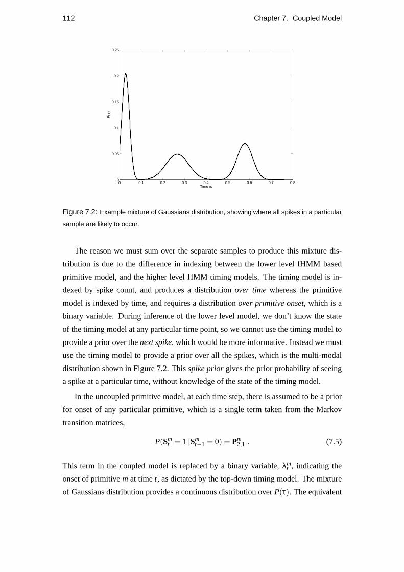
112 Chapter 7. Coupled Model
0 0.1 0.2 0.3 0.4 0.5 0.6 0.7 0.80
0.05
0.1
0.15
0.2
0.25
Time /s
P(τ
)
Figure 7.2: Example mixture of Gaussians distribution, showing where all spikes in a particular
sample are likely to occur.
The reason we must sum over the separate samples to produce this mixture dis-
tribution is due to the difference in indexing between the lower level fHMM based
primitive model, and the higher level HMM timing models. The timing model is in-
dexed by spike count, and produces a distributionover timewhereas the primitive
model is indexed by time, and requires a distributionover primitive onset, which is a
binary variable. During inference of the lower level model, we don’t know the state
of the timing model at any particular time point, so we cannot use the timing model to
provide a prior over thenext spike, which would be more informative. Instead we must
use the timing model to provide a prior over all the spikes, which is the multi-modal
distribution shown in Figure 7.2. Thisspike priorgives the prior probability of seeing
a spike at a particular time, without knowledge of the state of the timing model.
In the uncoupled primitive model, at each time step, there is assumed to be a prior
for onset of any particular primitive, which is a single term taken from the Markov
transition matrices,
P(Smt = 1|Sm
t−1 = 0) = Pm2,1 . (7.5)
This term in the coupled model is replaced by a binary variable,λmt , indicating the
onset of primitivem at timet, as dictated by the top-down timing model. The mixture
of Gaussians distribution provides a continuous distribution overP(τ). The equivalent
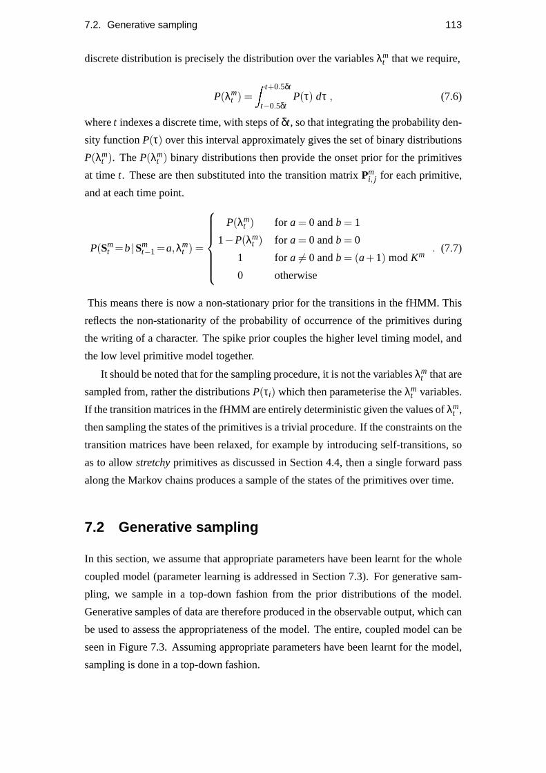
7.2. Generative sampling 113
discrete distribution is precisely the distribution over the variablesλmt that we require,
P(λmt ) =
Z t+0.5δt
t−0.5δtP(τ) dτ , (7.6)
wheret indexes a discrete time, with steps ofδt, so that integrating the probability den-
sity functionP(τ) over this interval approximately gives the set of binary distributions
P(λmt ). TheP(λm
t ) binary distributions then provide the onset prior for the primitives
at timet. These are then substituted into the transition matrixPmi, j for each primitive,
and at each time point.
P(Smt =b|Sm
t−1=a,λmt ) =
P(λm
t ) for a = 0 andb = 1
1−P(λmt ) for a = 0 andb = 0
1 for a 6= 0 andb = (a+1) modKm
0 otherwise
. (7.7)
This means there is now a non-stationary prior for the transitions in the fHMM. This
reflects the non-stationarity of the probability of occurrence of the primitives during
the writing of a character. The spike prior couples the higher level timing model, and
the low level primitive model together.
It should be noted that for the sampling procedure, it is not the variablesλmt that are
sampled from, rather the distributionsP(τi) which then parameterise theλmt variables.
If the transition matrices in the fHMM are entirely deterministic given the values ofλmt ,
then sampling the states of the primitives is a trivial procedure. If the constraints on the
transition matrices have been relaxed, for example by introducing self-transitions, so
as to allowstretchyprimitives as discussed in Section 4.4, then a single forward pass
along the Markov chains produces a sample of the states of the primitives over time.
7.2 Generative sampling
In this section, we assume that appropriate parameters have been learnt for the whole
coupled model (parameter learning is addressed in Section 7.3). For generative sam-
pling, we sample in a top-down fashion from the prior distributions of the model.
Generative samples of data are therefore produced in the observable output, which can
be used to assess the appropriateness of the model. The entire, coupled model can be
seen in Figure 7.3. Assuming appropriate parameters have been learnt for the model,
sampling is done in a top-down fashion.
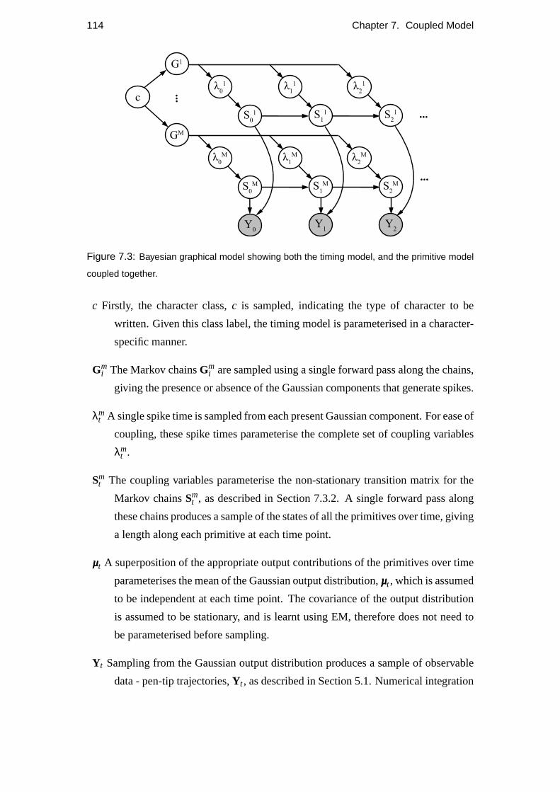
114 Chapter 7. Coupled Model
Figure 7.3: Bayesian graphical model showing both the timing model, and the primitive model
coupled together.
c Firstly, the character class,c is sampled, indicating the type of character to be
written. Given this class label, the timing model is parameterised in a character-
specific manner.
Gmi The Markov chainsGm
i are sampled using a single forward pass along the chains,
giving the presence or absence of the Gaussian components that generate spikes.
λmt A single spike time is sampled from each present Gaussian component. For ease of
coupling, these spike times parameterise the complete set of coupling variables
λmt .
Smt The coupling variables parameterise the non-stationary transition matrix for the
Markov chainsSmt , as described in Section 7.3.2. A single forward pass along
these chains produces a sample of the states of all the primitives over time, giving
a length along each primitive at each time point.
µµµt A superposition of the appropriate output contributions of the primitives over time
parameterises the mean of the Gaussian output distribution,µµµt , which is assumed
to be independent at each time point. The covariance of the output distribution
is assumed to be stationary, and is learnt using EM, therefore does not need to
be parameterised before sampling.
Yt Sampling from the Gaussian output distribution produces a sample of observable
data - pen-tip trajectories,Yt , as described in Section 5.1. Numerical integration

7.3. Inference 115
of these trajectories produces character samples, such as those seen in Section
7.4.
7.3 Inference
The parameters for the coupled model are difficult to learn as the model is quite large,
and multi layered. A variational approximation to the posterior distribution is used to
infer the state of the model, whilst the parameter updates are done as if the model con-
sisted of the two separate models, the fHMM primitive model and the HMM timing
model, where the whole model is coupled together with the spike prior. The infer-
ence is an iterative procedure, with several adjustable constants. This section gives a
description of how the inference was done algorithmically.
To clarify, the low level primitive model is a single fHMM model, and will be
referred to as the primitive model. The higher level timing model is a set ofM HMM
models, one for each primitive. This collection of HMMs will be referred to as the
timing model.
The inference of the timing model is much faster than the primitive model infer-
ence, due to the difference in indexing. The primitive model is indexed by time, and
therefore, in a typical character sample, the primitive model will have around 100 sam-
ples, whereas the timing model is indexed by spike count, and for a typical character
sample, there are around 2 spikes for each primitive.
7.3.1 Inference order
Parameter initialisations
All parameters are initialised to likely values. Output covariance is initialised to data
covariance. Primitive shapes are taken from sections of data averaged over the charac-
ter samples. Onset probabilities are initialised to 1/T whereT is the average length of
a character sample. The timing model component means are initialised using a simple
one dimensional local maxima finding algorithm based on the pool of all the spike tim-
ing data. The variance of the clusters is initialised to the variance of a greedy absolute
classification of the data. The transition parameters are initialised to values reflecting
this initial data classification.
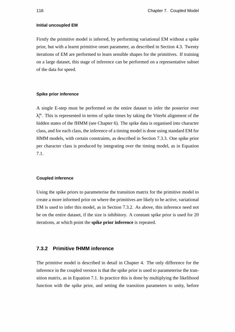
116 Chapter 7. Coupled Model
Initial uncoupled EM
Firstly the primitive model is inferred, by performing variational EM without a spike
prior, but with a learnt primitive onset parameter, as described in Section 4.3. Twenty
iterations of EM are performed to learn sensible shapes for the primitives. If training
on a large dataset, this stage of inference can be performed on a representative subset
of the data for speed.
Spike prior inference
A single E-step must be performed on the entire dataset to infer the posterior over
λmt . This is represented in terms of spike times by taking the Viterbi alignment of the
hidden states of the fHMM (see Chapter 6). The spike data is organised into character
class, and for each class, the inference of a timing model is done using standard EM for
HMM models, with certain constraints, as described in Section 7.3.3. One spike prior
per character class is produced by integrating over the timing model, as in Equation
7.1.
Coupled inference
Using the spike priors to parameterise the transition matrix for the primitive model to
create a more informed prior on where the primitives are likely to be active, variational
EM is used to infer this model, as in Section 7.3.2. As above, this inference need not
be on the entire dataset, if the size is inhibitory. A constant spike prior is used for 20
iterations, at which point thespike prior inference is repeated.
7.3.2 Primitive fHMM inference
The primitive model is described in detail in Chapter 4. The only difference for the
inference in the coupled version is that the spike prior is used to parameterise the tran-
sition matrix, as in Equation 7.1. In practice this is done by multiplying the likelihood
function with the spike prior, and setting the transition parameters to unity, before
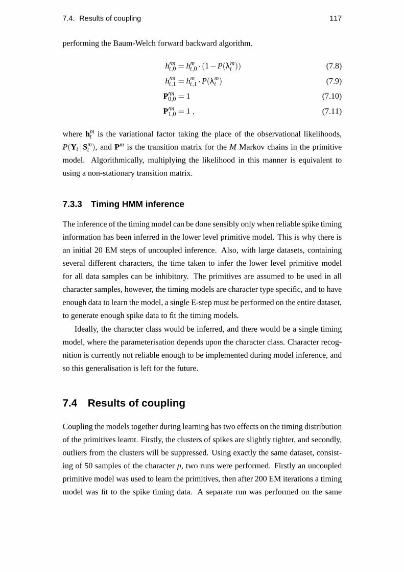
7.4. Results of coupling 117
performing the Baum-Welch forward backward algorithm.
h′mt,0 = hmt,0 · (1−P(λm
t )) (7.8)
h′mt,1 = hmt,1 ·P(λm
t ) (7.9)
P′m0,0 = 1 (7.10)
P′m1,0 = 1 , (7.11)
wherehmt is the variational factor taking the place of the observational likelihoods,
P(Yt |Smt ), andPm is the transition matrix for theM Markov chains in the primitive
model. Algorithmically, multiplying the likelihood in this manner is equivalent to
using a non-stationary transition matrix.
7.3.3 Timing HMM inference
The inference of the timing model can be done sensibly only when reliable spike timing
information has been inferred in the lower level primitive model. This is why there is
an initial 20 EM steps of uncoupled inference. Also, with large datasets, containing
several different characters, the time taken to infer the lower level primitive model
for all data samples can be inhibitory. The primitives are assumed to be used in all
character samples, however, the timing models are character type specific, and to have
enough data to learn the model, a single E-step must be performed on the entire dataset,
to generate enough spike data to fit the timing models.
Ideally, the character class would be inferred, and there would be a single timing
model, where the parameterisation depends upon the character class. Character recog-
nition is currently not reliable enough to be implemented during model inference, and
so this generalisation is left for the future.
7.4 Results of coupling
Coupling the models together during learning has two effects on the timing distribution
of the primitives learnt. Firstly, the clusters of spikes are slightly tighter, and secondly,
outliers from the clusters will be suppressed. Using exactly the same dataset, consist-
ing of 50 samples of the characterp, two runs were performed. Firstly an uncoupled
primitive model was used to learn the primitives, then after 200 EM iterations a timing
model was fit to the spike timing data. A separate run was performed on the same
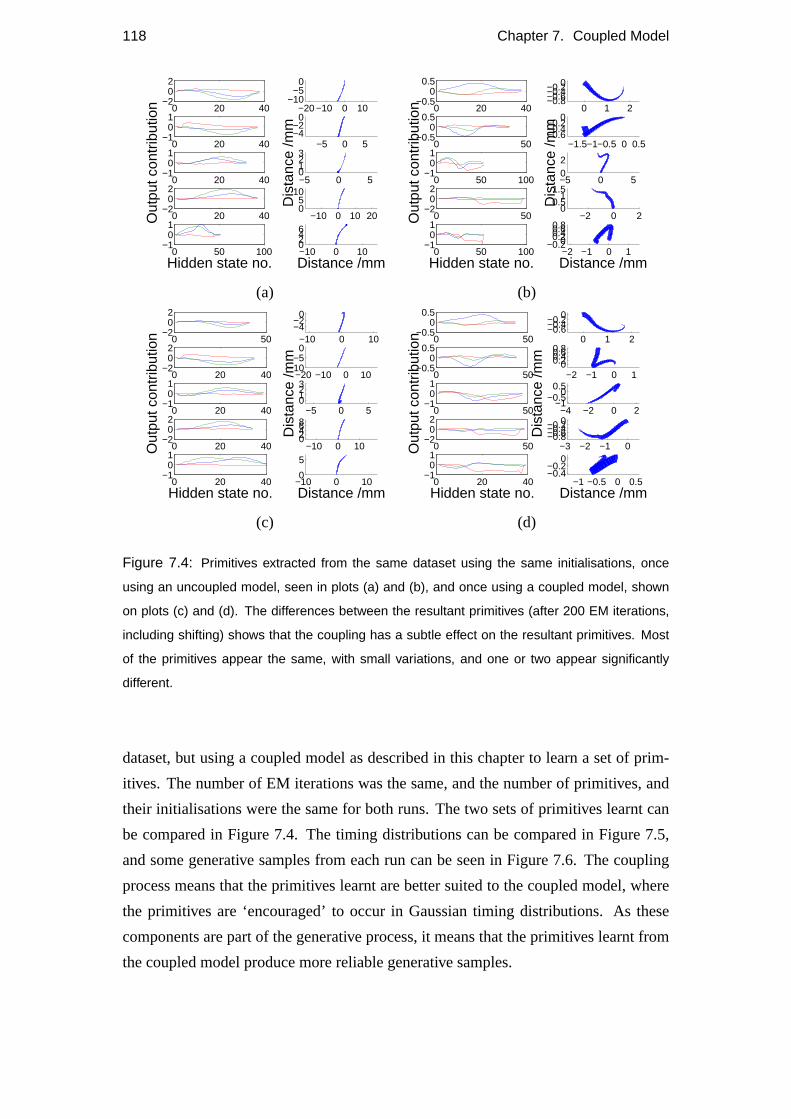
118 Chapter 7. Coupled Model
0 20 40−2
02
−20 −10 0 10−10
−50
0 20 40−1
01
−5 0 5−4−2
0
0 20 40−1
01
Out
put c
ontr
ibut
ion
−5 0 50123
Dis
tanc
e /m
m
0 20 40−2
02
−10 0 10 2005
10
0 50 100−1
01
Hidden state no.−10 0 100246
Distance /mm
0 20 40−0.5
00.5
0 1 2−0.8−0.6−0.4−0.20
0 50−0.5
00.5
−1.5−1−0.5 0 0.5−0.6−0.4−0.2
0
0 50 100−1
01
Out
put c
ontr
ibut
ion
−5 0 502
Dis
tanc
e /m
m
0 50−2
02
−2 0 20
0.51
1.5
0 50 100−1
01
Hidden state no.−2 −1 0 1
−0.200.20.40.60.8
Distance /mm
(a) (b)
0 50−2
02
−10 0 10−4−2
0
0 20 40−2
02
−20 −10 0 10−10
−50
0 20 40−1
01
Out
put c
ontr
ibut
ion
−5 0 50123
Dis
tanc
e /m
m
0 20 40−2
02
−10 0 1002468
0 20 40−1
01
Hidden state no.−10 0 100
5
Distance /mm
0 50−0.5
00.5
0 1 2−0.6−0.4−0.20
0 50−0.5
00.5
−2 −1 0 100.20.40.60.8
0 50−1
01
Out
put c
ontr
ibut
ion
−4 −2 0 2−1
−0.50
0.5
Dis
tanc
e /m
m
0 50−2
02
−3 −2 −1 0−0.8−0.6−0.4−0.20
0 20 40−1
01
Hidden state no.−1 −0.5 0 0.5
−0.4−0.2
0
Distance /mm
(c) (d)
Figure 7.4: Primitives extracted from the same dataset using the same initialisations, once
using an uncoupled model, seen in plots (a) and (b), and once using a coupled model, shown
on plots (c) and (d). The differences between the resultant primitives (after 200 EM iterations,
including shifting) shows that the coupling has a subtle effect on the resultant primitives. Most
of the primitives appear the same, with small variations, and one or two appear significantly
different.
dataset, but using a coupled model as described in this chapter to learn a set of prim-
itives. The number of EM iterations was the same, and the number of primitives, and
their initialisations were the same for both runs. The two sets of primitives learnt can
be compared in Figure 7.4. The timing distributions can be compared in Figure 7.5,
and some generative samples from each run can be seen in Figure 7.6. The coupling
process means that the primitives learnt are better suited to the coupled model, where
the primitives are ‘encouraged’ to occur in Gaussian timing distributions. As these
components are part of the generative process, it means that the primitives learnt from
the coupled model produce more reliable generative samples.
7.4. Results of coupling 119
0 0.2 0.4 0.6 0.8
1
2
3
4
5
6
7
8
9
10
Time /s
Prim
itive
num
ber
p
0 0.2 0.4 0.6 0.8
1
2
3
4
5
6
7
8
9
10
Time /s
Prim
itive
num
ber
p
Figure 7.5: Timing distribution of the primitives seen in Figure 7.4. The left plot shows the
timing distribution of primitives inferred for the uncoupled run, and the right plot for the coupled
run. The effect of coupling, as can be seen here, is to tighten the spike scatter towards the
Gaussian components, and to suppress outliers. It should be noted that this will only occur if
the model is ‘unsure’ that the outlier should exist. There are still outliers present in the coupled
model, but the occurrence of the primitive at that particular point was important enough for the
model to keep the outlier.
−10 0 10−10
−50
−10 0 10−15−10
−50
−10 0 10−15−10
−50
−10 0 10−10
−50
Dis
tanc
e /m
m
−10 0 10−15−10
−50
−10 0 10−15−10
−50
−10 0 10 20−15−10
−50
−10 0 10−15−10
−50
−10 0 10−15−10
−50
−10 0 10−10
−50
−10 0 10−15−10
−50
Distance /mm−10 0 10
−15−10
−50
−10 0 10−10
−505
−10 0 10
−10−5
0
−10 0 10−15−10
−50
−10 0 10
−10−5
0
Dis
tanc
e /m
m
−10 0 10−15−10
−50
−10 0 10−15−10
−50
−10 0 10−15−10
−50
−10 0 10−10
−50
−10 0 10−15−10
−50
−10 0 10−15−10
−50
−10 0 10−15−10
−50
Distance /mm−10 0 10
−15−10
−50
Figure 7.6: 12 generative samples from two separate runs with the same initialisations. The left
plot shows an uncoupled run, and the right plot shows a coupled run. The process of coupling
means that the generative samples, (which are produced from a coupled model in any case)
are generally better.
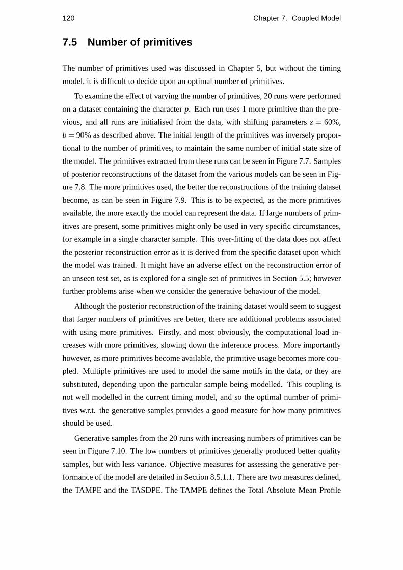
120 Chapter 7. Coupled Model
7.5 Number of primitives
The number of primitives used was discussed in Chapter 5, but without the timing
model, it is difficult to decide upon an optimal number of primitives.
To examine the effect of varying the number of primitives, 20 runs were performed
on a dataset containing the characterp. Each run uses 1 more primitive than the pre-
vious, and all runs are initialised from the data, with shifting parametersz = 60%,
b = 90% as described above. The initial length of the primitives was inversely propor-
tional to the number of primitives, to maintain the same number of initial state size of
the model. The primitives extracted from these runs can be seen in Figure 7.7. Samples
of posterior reconstructions of the dataset from the various models can be seen in Fig-
ure 7.8. The more primitives used, the better the reconstructions of the training dataset
become, as can be seen in Figure 7.9. This is to be expected, as the more primitives
available, the more exactly the model can represent the data. If large numbers of prim-
itives are present, some primitives might only be used in very specific circumstances,
for example in a single character sample. This over-fitting of the data does not affect
the posterior reconstruction error as it is derived from the specific dataset upon which
the model was trained. It might have an adverse effect on the reconstruction error of
an unseen test set, as is explored for a single set of primitives in Section 5.5; however
further problems arise when we consider the generative behaviour of the model.
Although the posterior reconstruction of the training dataset would seem to suggest
that larger numbers of primitives are better, there are additional problems associated
with using more primitives. Firstly, and most obviously, the computational load in-
creases with more primitives, slowing down the inference process. More importantly
however, as more primitives become available, the primitive usage becomes more cou-
pled. Multiple primitives are used to model the same motifs in the data, or they are
substituted, depending upon the particular sample being modelled. This coupling is
not well modelled in the current timing model, and so the optimal number of primi-
tives w.r.t. the generative samples provides a good measure for how many primitives
should be used.
Generative samples from the 20 runs with increasing numbers of primitives can be
seen in Figure 7.10. The low numbers of primitives generally produced better quality
samples, but with less variance. Objective measures for assessing the generative per-
formance of the model are detailed in Section 8.5.1.1. There are two measures defined,
the TAMPE and the TASDPE. The TAMPE defines the Total Absolute Mean Profile
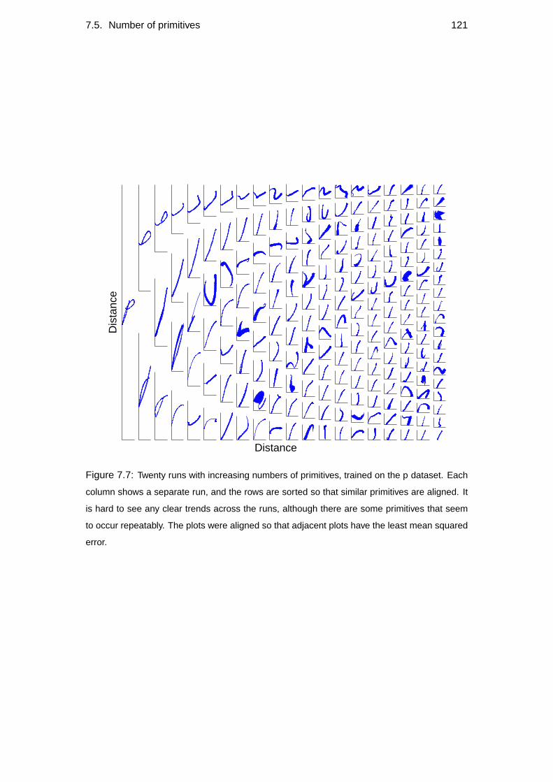
7.5. Number of primitives 121
Dis
tanc
e
Distance
Figure 7.7: Twenty runs with increasing numbers of primitives, trained on the p dataset. Each
column shows a separate run, and the rows are sorted so that similar primitives are aligned. It
is hard to see any clear trends across the runs, although there are some primitives that seem
to occur repeatably. The plots were aligned so that adjacent plots have the least mean squared
error.
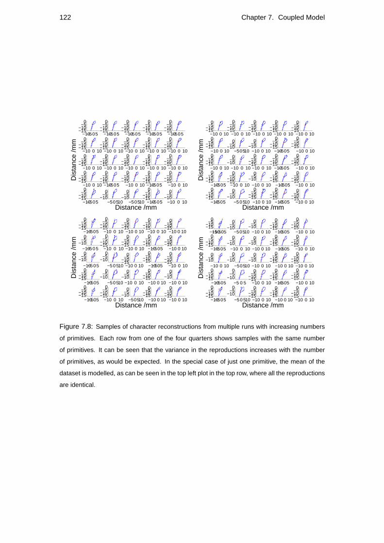
122 Chapter 7. Coupled Model
−10−505−15−10
−50
−10−505−15−10
−50
−10−505−15−10
−50
−10−505−15−10
−50
−10−505−15−10
−50
−10 0 10−15−10
−50
−10 0 10−15−10
−50
−10 0 10−15−10
−50
−10 0 10−15−10
−50
−10 0 10−15−10
−50
−10 0 10−15−10
−50
Dis
tanc
e /m
m
−10 0 10−15−10
−50
−10 0 10−15−10
−50
−10 0 10−15−10
−50
−10 0 10−15−10
−50
−10 0 10−15−10
−50
−10−505−15−10
−50
−10 0 10−15−10
−50
−10−505−15−10
−50
−10 0 10−15−10
−50
−10−505−15−10
−50
−50510−10
−50
−50510−10
−50
Distance /mm−10−505
−15−10
−50
−10 0 10−10
−50
−10 0 10−15−10
−50
−10 0 10−15−10
−50
−10 0 10−15−10
−50
−10 0 10−15−10
−50
−10 0 10−15−10
−50
−10 0 10−15−10
−50
−50510−10
−50
−10 0 10−10
−50
−10−505−15−10
−50
−10 0 10−15−10
−50
−10 0 10−15−10
−50
Dis
tanc
e /m
m
−10 0 10−10
−50
−10 0 10−15−10
−50
−10−505−15−10
−50
−10 0 10−15−10
−50
−10−505−15−10
−50
−10 0 10−15−10
−50
−10 0 10−10
−50
−10−505−15−10
−50
−10 0 10−15−10
−50
−10−505−15−10
−50
−5 0 510−10
−50
−10 0 10−15−10
−50
Distance /mm−10−505
−15−10
−50
−10 0 10−15−10
−50
−10−505−15−10
−50
−10 0 10−15−10
−50
−10 0 10−15−10
−50
−10 0 10−15−10
−50
−10 0 10−15−10−50
−10−5 0 5−10
−50
−10 0 10−15−10
−50
−10 0 10−15−10
−50
−10−505−15−10
−50
−10 0 10−15−10−50
−10−505−10
−50
Dis
tanc
e /m
m
−5 0 510−10
−50
−10 0 10−15−10−50
−10−505−15−10
−50
−10 0 10−15−10
−50
−10−505−15−10
−50
−50510−10
−50
−10 0 10−10
−50
−10 0 10−15−10−50
−10 0 10−10
−50
−10−505−15−10
−50
−10 0 10−15−10
−50
−50510−10
−50
Distance /mm−10 0 10
−15−10−50
−10 0 10−15−10
−50
−15−10−505−15−10−50
−50510−10
−50
−10 0 10−10
−50
−10−505−15−10
−50
−10 0 10−15−10
−50
−10−505−15−10
−50
−10 0 10−10
−50
−10 0 10−10−5
0
−10−505−15−10−50
−10 0 10−15−10
−50
−10 0 10−10
−50
Dis
tanc
e /m
m
−50510−10
−50
−10 0 10−10
−50
−10 0 10−15−10−50
−10 0 10−15−10
−50
−10−505−15−10
−50
−5 0 5−10
−50
−10 0 10−15−10
−50
−10−505−15−10
−50
−10 0 10−15−10
−50
−10−505−15−10
−50
−5 0 510−10
−50
−10 0 10−15−10
−50
Distance /mm−10 0 10
−15−10−50
−10 0 10−15−10
−50
Figure 7.8: Samples of character reconstructions from multiple runs with increasing numbers
of primitives. Each row from one of the four quarters shows samples with the same number
of primitives. It can be seen that the variance in the reproductions increases with the number
of primitives, as would be expected. In the special case of just one primitive, the mean of the
dataset is modelled, as can be seen in the top left plot in the top row, where all the reproductions
are identical.
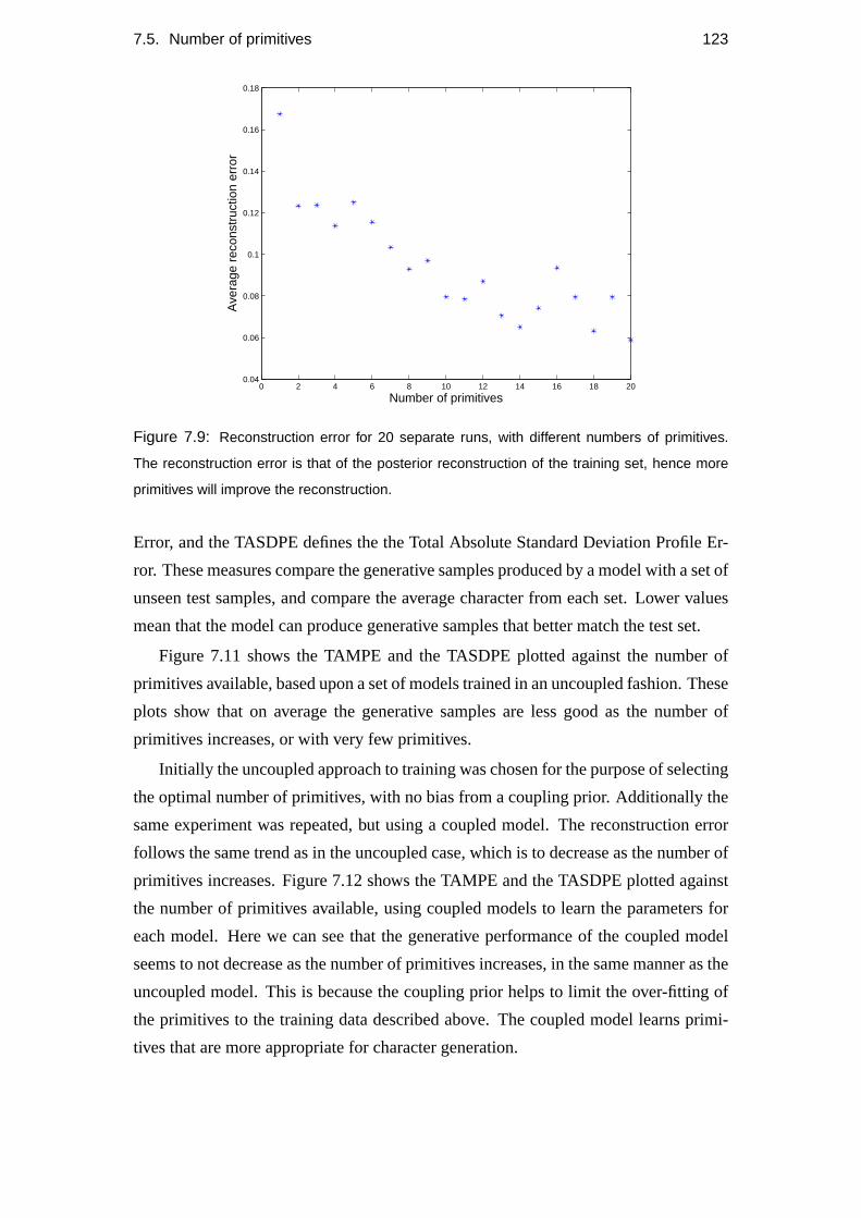
7.5. Number of primitives 123
0 2 4 6 8 10 12 14 16 18 200.04
0.06
0.08
0.1
0.12
0.14
0.16
0.18
Number of primitives
Ave
rage
rec
onst
ruct
ion
erro
r
Figure 7.9: Reconstruction error for 20 separate runs, with different numbers of primitives.
The reconstruction error is that of the posterior reconstruction of the training set, hence more
primitives will improve the reconstruction.
Error, and the TASDPE defines the the Total Absolute Standard Deviation Profile Er-
ror. These measures compare the generative samples produced by a model with a set of
unseen test samples, and compare the average character from each set. Lower values
mean that the model can produce generative samples that better match the test set.
Figure 7.11 shows the TAMPE and the TASDPE plotted against the number of
primitives available, based upon a set of models trained in an uncoupled fashion. These
plots show that on average the generative samples are less good as the number of
primitives increases, or with very few primitives.
Initially the uncoupled approach to training was chosen for the purpose of selecting
the optimal number of primitives, with no bias from a coupling prior. Additionally the
same experiment was repeated, but using a coupled model. The reconstruction error
follows the same trend as in the uncoupled case, which is to decrease as the number of
primitives increases. Figure 7.12 shows the TAMPE and the TASDPE plotted against
the number of primitives available, using coupled models to learn the parameters for
each model. Here we can see that the generative performance of the coupled model
seems to not decrease as the number of primitives increases, in the same manner as the
uncoupled model. This is because the coupling prior helps to limit the over-fitting of
the primitives to the training data described above. The coupled model learns primi-
tives that are more appropriate for character generation.
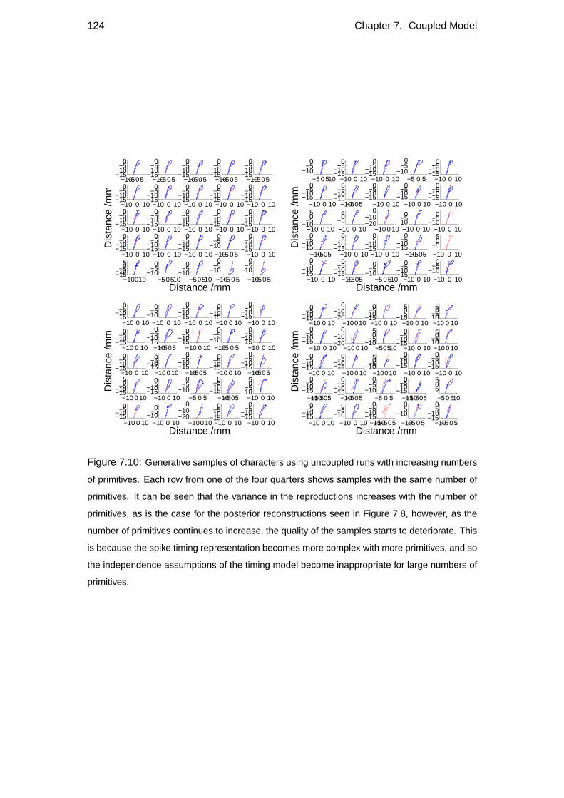
124 Chapter 7. Coupled Model
−10−505−15−10
−50
−10−505−15−10
−50
−10−505−15−10
−50
−10−505−15−10
−50
−10−505−15−10
−50
−10 0 10−15−10
−50
−10 0 10−15−10
−50
−10 0 10−15−10
−50
−10 0 10−15−10
−50
−10 0 10−15−10
−50
−10 0 10−15−10
−50
Dis
tanc
e /m
m
−10 0 10−15−10
−50
−10 0 10−15−10
−50
−10 0 10−15−10
−50
−10 0 10−15−10
−50
−10 0 10−15−10
−50
−10 0 10−15−10
−50
−10 0 10−15−10
−50
−10−5 0 5−10
−50
−10 0 10−15−10
−50
−10010−15−10−50
5
−50510−10
−50
−50510−10
−50
Distance /mm−10−5 0 5
−10−5
0
−10−5 0 5−10
−50
−50 510−10
−50
−10 0 10−15−10
−50
−10 0 10−15−10
−50
−5 0 5−10
−50
−10 0 10−15−10
−50
−10 0 10−15−10
−50
−10−505−15−10
−50
−10 0 10−15−10
−50
−10 0 10−15−10−50
−10 0 10−15−10
−50
−10 0 10−10
−505
Dis
tanc
e /m
m
−10 0 10−5
05
−10 0 10−20−10
0
−10 0 10−10
−50
−10 0 10−10
−50
−10−505−15−10
−50
−10 0 10−15−10
−50
−10 0 10−15−10
−50
−10−505−15−10
−50
−10 0 10−5
05
−10 0 10−15−10
−50
−10−505−15−10
−50
−50510−10
−50
Distance /mm−10 0 10
−15−10
−50
−10 0 10−10
−50
−10 0 10−15−10
−50
−10 0 10−10
−50
−10 0 10−15−10
−50
−10 0 10−15−10−50
−10 0 10−15−10
−50
−10 0 10−15−10−50
−10−505−15−10
−50
−10 0 10−15−10−50
−10−5 0 5−10
−50
−10 0 10−15−10
−50
−10 0 10−15−10
−50
Dis
tanc
e /m
m
−10010−15−10−50
−10−505−15−10
−50
−10 0 10−15−10−50
−10−505−15−10
−50
−10 0 10−15−10−50
5
−10 0 10−15−10−50
−5 0 5−10
−50
−10−505−15−10
−50
−10 0 10−10
−505
−10 0 10−15−10−50
−10 0 10−10
−50
−10010−20−10
0
Distance /mm−10 0 10
−15−10
−50
−10 0 10−15−10
−50
−10 0 10−15−10−50
−10010−20−10
0
−10 0 10−15−10−50
−10 0 10−10−50
5
−10 0 10−10−50
5
−10 0 10−15−10
−50
−10 0 10−20−10
0
−50510−10
−505
−10 0 10−15−10
−50
−10 0 10−10−50
5
−10 0 10−15−10−50
Dis
tanc
e /m
m
−10 0 10−15−10−50
−10010−10−50
5
−10 0 10−15−10−50
−10 0 10−15−10
−50
−15−10−505−15−10−50
−10−505−15−10
−50
−5 0 5−10
−50
−15−10−505−15−10
−50
−50510−5
05
−10 0 10−15−10−50
−10 0 10−10
−50
−15−10−505−15−10
−50
Distance /mm−10−5 0 5
−10−5
0
−10−505−15−10
−50
Figure 7.10: Generative samples of characters using uncoupled runs with increasing numbers
of primitives. Each row from one of the four quarters shows samples with the same number of
primitives. It can be seen that the variance in the reproductions increases with the number of
primitives, as is the case for the posterior reconstructions seen in Figure 7.8, however, as the
number of primitives continues to increase, the quality of the samples starts to deteriorate. This
is because the spike timing representation becomes more complex with more primitives, and so
the independence assumptions of the timing model become inappropriate for large numbers of
primitives.
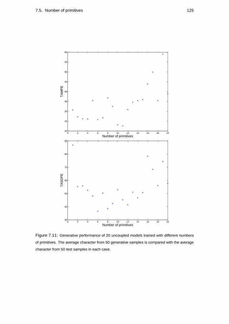
7.5. Number of primitives 125
0 2 4 6 8 10 12 14 16 18 2020
25
30
35
40
45
50
55
60
Number of primitives
TA
MP
E
0 2 4 6 8 10 12 14 16 18 2030
40
50
60
70
80
90
Number of primitives
TA
SD
PE
Figure 7.11: Generative performance of 20 uncoupled models trained with different numbers
of primitives. The average character from 50 generative samples is compared with the average
character from 50 test samples in each case.
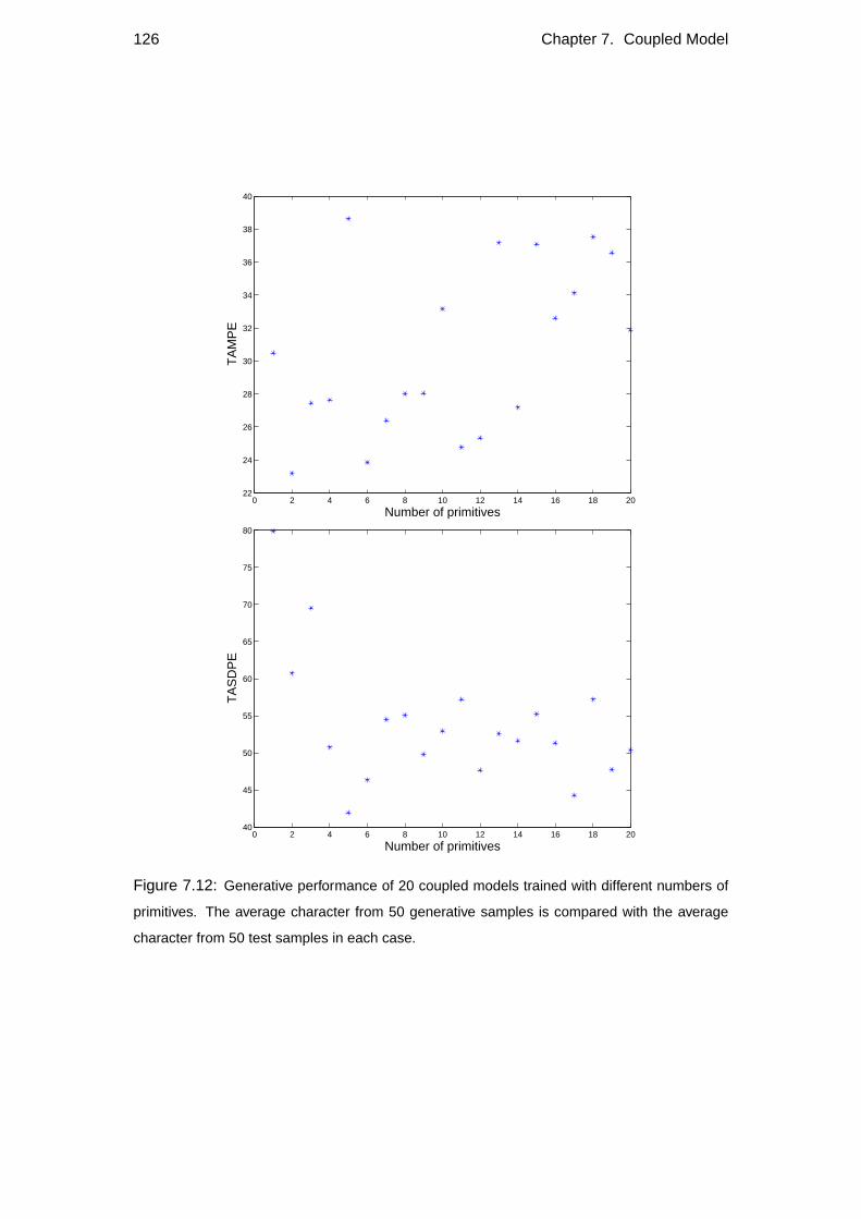
126 Chapter 7. Coupled Model
0 2 4 6 8 10 12 14 16 18 2022
24
26
28
30
32
34
36
38
40
Number of primitives
TA
MP
E
0 2 4 6 8 10 12 14 16 18 2040
45
50
55
60
65
70
75
80
Number of primitives
TA
SD
PE
Figure 7.12: Generative performance of 20 coupled models trained with different numbers of
primitives. The average character from 50 generative samples is compared with the average
character from 50 test samples in each case.

7.5. Number of primitives 127
All these results contain a lot of noise. This is partly because the training set sizes
were relatively small, to speed up the experiment, which required separate training on
each dataset. In general however, it can be seen that the optimal number of primitives
for a single character should be around 6-15. With multiple characters in the dataset,
the number of primitives required increases, but sub-linearly to the number of character
types. It was found empirically that 5-10 primitives model a single character well,
whilst 10-15 should be used for sets of 3 to 5 characters. The largest set of character
types used was 20, which can be modelled with 20 primitives.

Chapter 8
Results
The past four chapters have described a handwriting model based upon the concept of
primitives. Chapters 4 and 5 give details of the lower level parts of this model, and
Chapters 6 and 7 examine possible higher level models and how the two models can
be coupled together allowing generalisation across character samples.
This chapter examines the results of generative experiments using the coupled
model. There are several ways to assess such experiments, and these are discussed.
The types of primitives extracted will be shown, and the possibility of these primitives
modelling thestyleof a person’s handwriting will be assessed in a simple case.
Additionally, the appropriateness of the model for different character types can be
used as a measure for character recognition. The discriminative performance of the
model is not taken into account during training or model design, and as such can be
thought of as a ‘free’ aspect of the model. The recognition accuracy for a simple case
is assessed.
Finally this chapter includes a discussion and assessment of how this model com-
pares to other handwriting models, and more general time series modelling systems.
A comparison to some alternative models is performed, and in particular an auditory
model based upon atomic signals will be examined.
8.1 Generative results
The model described in previous chapters is a generative model, which has a set of pa-
rameters which describe the probabilistic operation of the model. These parameters are
learnt from a training dataset, using a variational expectation maximisation procedure
as described in Section 4.3. Given a set of learnt parameters, the model then can gener-
129
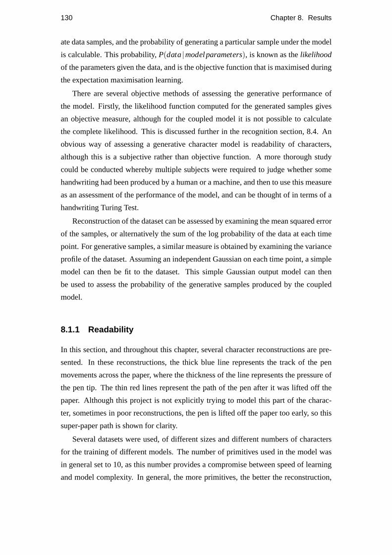
130 Chapter 8. Results
ate data samples, and the probability of generating a particular sample under the model
is calculable. This probability,P(data|modelparameters), is known as thelikelihood
of the parameters given the data, and is the objective function that is maximised during
the expectation maximisation learning.
There are several objective methods of assessing the generative performance of
the model. Firstly, the likelihood function computed for the generated samples gives
an objective measure, although for the coupled model it is not possible to calculate
the complete likelihood. This is discussed further in the recognition section, 8.4. An
obvious way of assessing a generative character model is readability of characters,
although this is a subjective rather than objective function. A more thorough study
could be conducted whereby multiple subjects were required to judge whether some
handwriting had been produced by a human or a machine, and then to use this measure
as an assessment of the performance of the model, and can be thought of in terms of a
handwriting Turing Test.
Reconstruction of the dataset can be assessed by examining the mean squared error
of the samples, or alternatively the sum of the log probability of the data at each time
point. For generative samples, a similar measure is obtained by examining the variance
profile of the dataset. Assuming an independent Gaussian on each time point, a simple
model can then be fit to the dataset. This simple Gaussian output model can then
be used to assess the probability of the generative samples produced by the coupled
model.
8.1.1 Readability
In this section, and throughout this chapter, several character reconstructions are pre-
sented. In these reconstructions, the thick blue line represents the track of the pen
movements across the paper, where the thickness of the line represents the pressure of
the pen tip. The thin red lines represent the path of the pen after it was lifted off the
paper. Although this project is not explicitly trying to model this part of the charac-
ter, sometimes in poor reconstructions, the pen is lifted off the paper too early, so this
super-paper path is shown for clarity.
Several datasets were used, of different sizes and different numbers of characters
for the training of different models. The number of primitives used in the model was
in general set to 10, as this number provides a compromise between speed of learning
and model complexity. In general, the more primitives, the better the reconstruction,
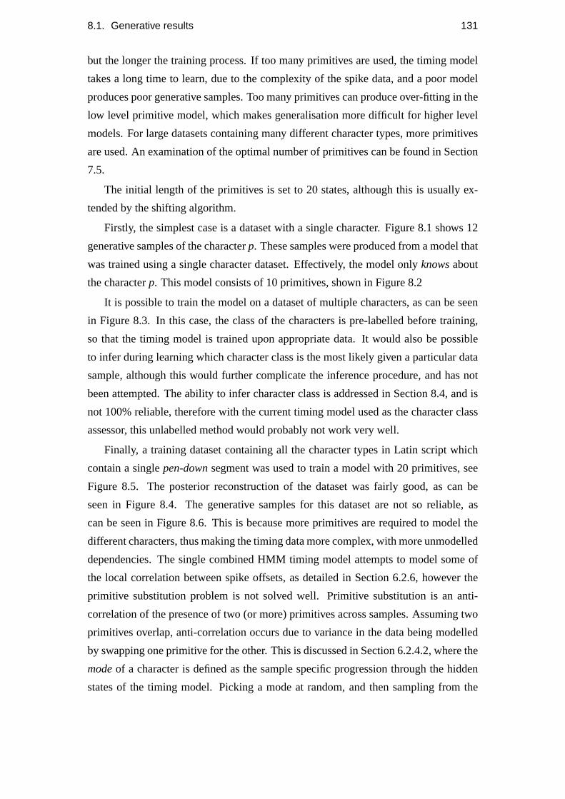
8.1. Generative results 131
but the longer the training process. If too many primitives are used, the timing model
takes a long time to learn, due to the complexity of the spike data, and a poor model
produces poor generative samples. Too many primitives can produce over-fitting in the
low level primitive model, which makes generalisation more difficult for higher level
models. For large datasets containing many different character types, more primitives
are used. An examination of the optimal number of primitives can be found in Section
7.5.
The initial length of the primitives is set to 20 states, although this is usually ex-
tended by the shifting algorithm.
Firstly, the simplest case is a dataset with a single character. Figure 8.1 shows 12
generative samples of the characterp. These samples were produced from a model that
was trained using a single character dataset. Effectively, the model onlyknowsabout
the characterp. This model consists of 10 primitives, shown in Figure 8.2
It is possible to train the model on a dataset of multiple characters, as can be seen
in Figure 8.3. In this case, the class of the characters is pre-labelled before training,
so that the timing model is trained upon appropriate data. It would also be possible
to infer during learning which character class is the most likely given a particular data
sample, although this would further complicate the inference procedure, and has not
been attempted. The ability to infer character class is addressed in Section 8.4, and is
not 100% reliable, therefore with the current timing model used as the character class
assessor, this unlabelled method would probably not work very well.
Finally, a training dataset containing all the character types in Latin script which
contain a singlepen-downsegment was used to train a model with 20 primitives, see
Figure 8.5. The posterior reconstruction of the dataset was fairly good, as can be
seen in Figure 8.4. The generative samples for this dataset are not so reliable, as
can be seen in Figure 8.6. This is because more primitives are required to model the
different characters, thus making the timing data more complex, with more unmodelled
dependencies. The single combined HMM timing model attempts to model some of
the local correlation between spike offsets, as detailed in Section 6.2.6, however the
primitive substitution problem is not solved well. Primitive substitution is an anti-
correlation of the presence of two (or more) primitives across samples. Assuming two
primitives overlap, anti-correlation occurs due to variance in the data being modelled
by swapping one primitive for the other. This is discussed in Section 6.2.4.2, where the
modeof a character is defined as the sample specific progression through the hidden
states of the timing model. Picking a mode at random, and then sampling from the
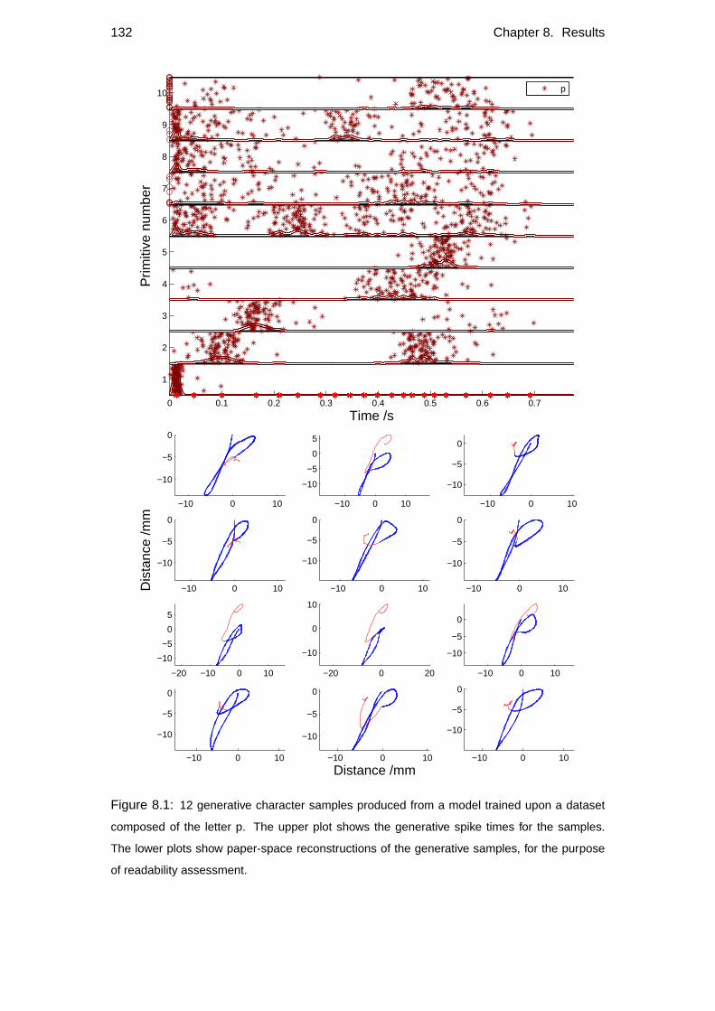
132 Chapter 8. Results
0 0.1 0.2 0.3 0.4 0.5 0.6 0.7
1
2
3
4
5
6
7
8
9
10
Time /s
Prim
itive
num
ber
p
−10 0 10
−10
−5
0
−10 0 10
−10
−5
0
5
−10 0 10
−10
−5
0
−10 0 10
−10
−5
0
Dis
tanc
e /m
m
−10 0 10
−10
−5
0
−10 0 10
−10
−5
0
−20 −10 0 10
−10
−5
0
5
−20 0 20
−10
0
10
−10 0 10
−10
−5
0
−10 0 10
−10
−5
0
−10 0 10
−10
−5
0
Distance /mm−10 0 10
−10
−5
0
Figure 8.1: 12 generative character samples produced from a model trained upon a dataset
composed of the letter p. The upper plot shows the generative spike times for the samples.
The lower plots show paper-space reconstructions of the generative samples, for the purpose
of readability assessment.
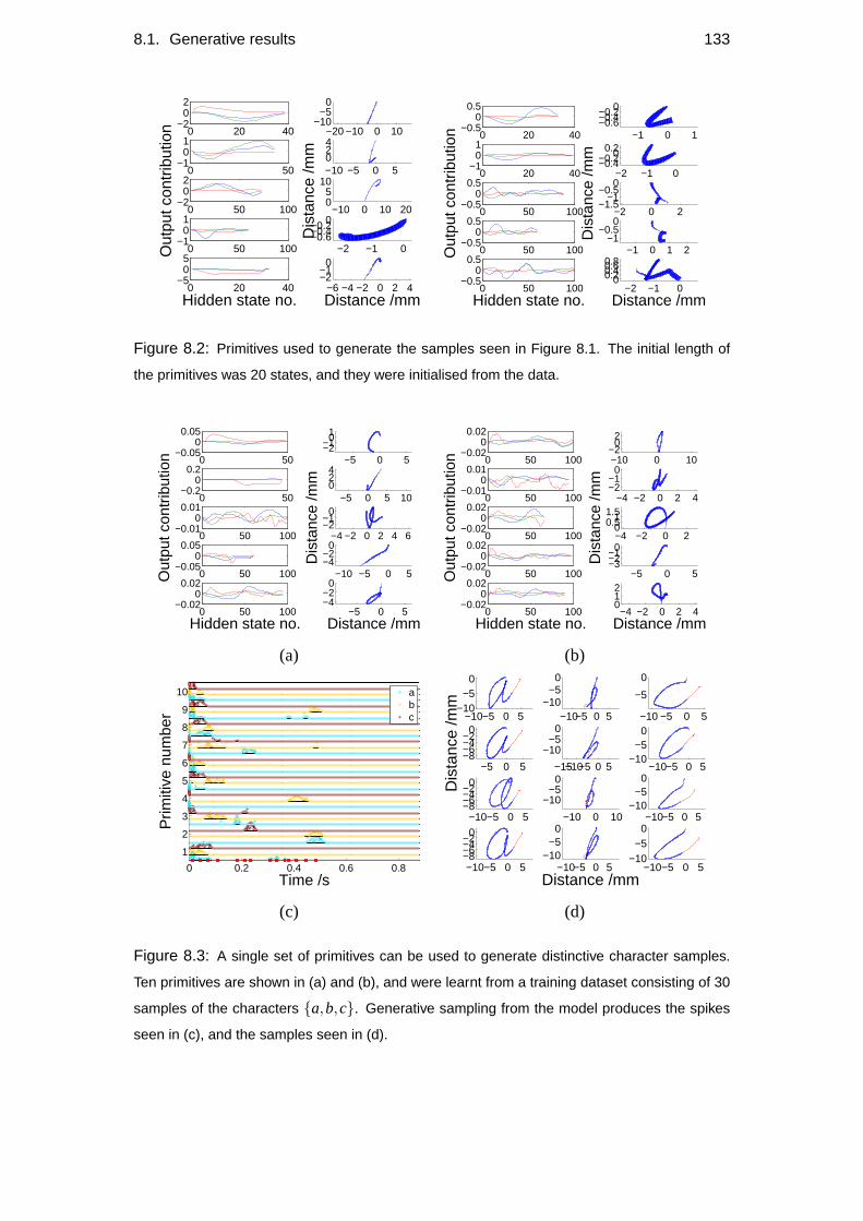
8.1. Generative results 133
0 20 40−2
02
−20 −10 0 10−10
−50
0 50−1
01
−10 −5 0 5024
0 50 100−2
02
Out
put c
ontr
ibut
ion
−10 0 10 2005
10
Dis
tanc
e /m
m
0 50 100−1
01
−2 −1 0−0.6−0.4−0.20
0 20 40−5
05
Hidden state no.−6 −4 −2 0 2 4
−2−1
0
Distance /mm
0 20 40−0.5
00.5
−1 0 1−0.6−0.4−0.20
0 20 40−1
01
−2 −1 0−0.4−0.20
0.2
0 50 100−0.5
00.5
Out
put c
ontr
ibut
ion
−2 0 2−1.5
−1−0.5
0
Dis
tanc
e /m
m
0 50 100−0.5
00.5
−1 0 1 2−1
−0.50
0 50 100−0.5
00.5
Hidden state no.−2 −1 0
00.20.40.60.8
Distance /mm
Figure 8.2: Primitives used to generate the samples seen in Figure 8.1. The initial length of
the primitives was 20 states, and they were initialised from the data.
0 50−0.05
00.05
−5 0 5−2−10
1
0 50−0.2
00.2
−5 0 5 10024
0 50 100−0.01
00.01
Out
put c
ontr
ibut
ion
−4 −2 0 2 4 6−2−1
0
Dis
tanc
e /m
m
0 50 100−0.05
00.05
−10 −5 0 5−4−2
0
0 50 100−0.02
00.02
Hidden state no.−5 0 5
−4−2
0
Distance /mm
0 50 100−0.02
00.02
−10 0 10−2
02
0 50 100−0.01
00.01
−4 −2 0 2 4−2−1
0
0 50 100−0.02
00.02
Out
put c
ontr
ibut
ion
−4 −2 0 200.51
1.5
Dis
tanc
e /m
m0 50 100
−0.020
0.02
−5 0 5−3−2−10
0 50 100−0.02
00.02
Hidden state no.−4 −2 0 2 4
012
Distance /mm
(a) (b)
0 0.2 0.4 0.6 0.8
1
2
3
4
5
6
7
8
9
10
Time /s
Prim
itive
num
ber
abc −10−5 0 5
−10−5
0
−10−5 0 5−10
−50
−10 −5 0 5
−5
0
−5 0 5−8−6−4−2
0
Dis
tanc
e /m
m
−15−10−5 0 5
−10−5
0
−10−5 0 5−10
−50
−10−5 0 5−8−6−4−20
−10 0 10
−10−5
0
−10−5 0 5−10
−50
−10−5 0 5−8−6−4−20
−10−5 0 5−10
−50
Distance /mm−10−5 0 5
−10−5
0
(c) (d)
Figure 8.3: A single set of primitives can be used to generate distinctive character samples.
Ten primitives are shown in (a) and (b), and were learnt from a training dataset consisting of 30
samples of the characters {a,b,c}. Generative sampling from the model produces the spikes
seen in (c), and the samples seen in (d).
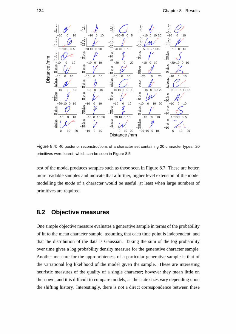
134 Chapter 8. Results
−10 0 10−6−4−20
24
−10 0 10
−10−5
0
−10−5 0 5−8−6−4−2
0
−10 0 10 20−5
05
−10 0 10−5
05
−15−10−5 0 5−10
−50
−20−10 0 10
−15−10
−50
−20−10 0 10−20−10
0
−5 0 5 1015−10
−50
−10 0 10−10
−50
−10 0 10−10
−50
−10 0 10
−10−5
0
−20 0 20−20−10
0
−10 0 10
−10−5
0
−20−10 0 10−15−10
−50
−10 0 10
−10−5
0
Dis
tanc
e /m
m
−10 0 10
−10−5
0
−10 0 10−10
−50
−20 0 20−15−10
−50
−10 0 10
−10−5
0
−10 0 10−6−4−20
24
−10 0 10−10
−50
−15−10−5 0 5−8−6−4−20
−10 0 10 20−5
05
−5 0 5 10 15−6−4−20
24
−20−10 0 10−15−10
−50
−10 0 10
−10−5
0
−10 0 10−10
−50
−10 0 10 20−10
−50
−10 0 10−10
−50
−10 0 10−10
−50
−10 0 10 20−15−10
−50
−20−10 0 10−15−10
−50
−10 0 10−10
−50
−15−10−5 0 5−10
−50
0 10 20−8−6−4−20
−10 0 10
−10−5
0
0 10 20
−505
Distance /mm−20−10 0 10
−15−10
−50
0 10 20−10
−50
Figure 8.4: 40 posterior reconstructions of a character set containing 20 character types. 20
primitives were learnt, which can be seen in Figure 8.5.
rest of the model produces samples such as those seen in Figure 8.7. These are better,
more readable samples and indicate that a further, higher level extension of the model
modelling themodeof a character would be useful, at least when large numbers of
primitives are required.
8.2 Objective measures
One simple objective measure evaluates a generative sample in terms of the probability
of fit to the mean character sample, assuming that each time point is independent, and
that the distribution of the data is Gaussian. Taking the sum of the log probability
over time gives a log probability density measure for the generative character sample.
Another measure for the appropriateness of a particular generative sample is that of
the variational log likelihood of the model given the sample. These are interesting
heuristic measures of the quality of a single character; however they mean little on
their own, and it is difficult to compare models, as the state sizes vary depending upon
the shifting history. Interestingly, there is not a direct correspondence between these

8.2. Objective measures 135
−6 −4 −2 0
−6
−4
−2
0
0 0.5 1
−1
−0.5
0
−1 0 1 2−1
0
1
2
−2 0 2−4
−2
0
0 2
−1
0
1
0 1 2 30
1
2
3
Dis
tanc
e /m
m
−1 0 1 2 3
−4
−2
0
0 1 2 3
−2
−1
0
0 2 40
2
4
6
−2 0 2 4
−2
0
2
−2 0 2
0
2
4
−3 −2 −1 0
−2
−1
0
1
−1 0 1−3
−2
−1
0
−1.5−1−0.5 0 0.5
−1
−0.5
0
0.5
−4 −2 0
−4
−2
0
−1 0 1
0
1
2
3
−1 0 1 2
−2
−1
0
1
−1 0 1 2 3
−1
0
1
2
Distance /mm−2 −1 0
−1
0
1
−4 −2 0 2
−6
−4
−2
0
Figure 8.5: 20 primitives learnt from a dataset containing 20 character types. The characters
with very little variance seem to be modelled more directly with individual primitives, such as the
c and the l.
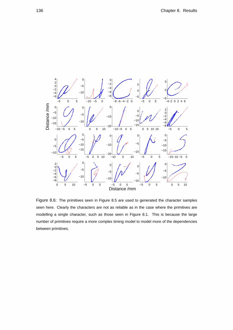
136 Chapter 8. Results
−5 0 5
−6−4−2
024
−10 −5 0
−10
−5
0
−8 −6 −4 −2 0
−8−6−4−2
0
−5 0 5
−5
0
5
−4−2 0 2 4 6−5
0
5
−10 −5 0 5
−15
−10
−5
0
Dis
tanc
e /m
m
0 5 10
−10
−5
0
−10 −5 0 5−20
−10
0
0 5 10 15−15
−10
−5
0
−5 0 5−8−6−4−2
02
−5 0 5
−10
−5
0
−5 0 5 10
−15
−10
−5
0
−10 0 10−20
−10
0
−5 0 5
−10
−5
0
−15−10 −5 0
−15
−10
−5
0
0 5 10
−8−6−4−2
02
−5 0 5
−10
−5
0
−5 0 5
−10
−5
0
Distance /mm−5 0 5
−10
−5
0
0 5 10
−10
−5
0
Figure 8.6: The primitives seen in Figure 8.5 are used to generated the character samples
seen here. Clearly the characters are not as reliable as in the case where the primitives are
modelling a single character, such as those seen in Figure 8.1. This is because the large
number of primitives require a more complex timing model to model more of the dependencies
between primitives.
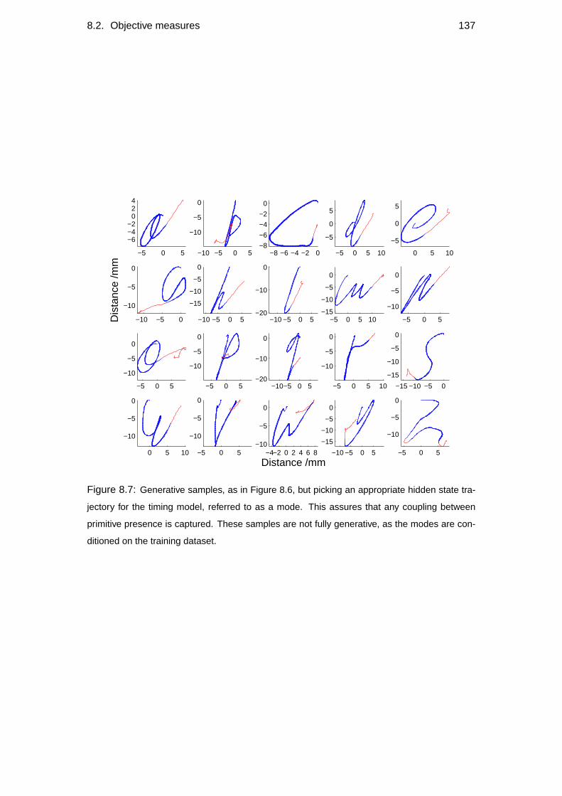
8.2. Objective measures 137
−5 0 5
−6−4−2
024
−10 −5 0 5
−10
−5
0
−8 −6 −4 −2 0−8
−6
−4
−2
0
−5 0 5 10
−5
0
5
0 5 10
−5
0
5
−10 −5 0
−10
−5
0
Dis
tanc
e /m
m
−10 −5 0 5
−15
−10
−5
0
−10 −5 0 5−20
−10
0
−5 0 5 10−15
−10
−5
0
−5 0 5
−10
−5
0
−5 0 5
−10
−5
0
−5 0 5
−10
−5
0
−10−5 0 5−20
−10
0
−5 0 5 10
−10
−5
0
−15 −10 −5 0
−15
−10
−5
0
0 5 10
−10
−5
0
−5 0 5
−10
−5
0
−4−2 0 2 4 6 8−10
−5
0
Distance /mm−10 −5 0 5
−15
−10
−5
0
−5 0 5
−10
−5
0
Figure 8.7: Generative samples, as in Figure 8.6, but picking an appropriate hidden state tra-
jectory for the timing model, referred to as a mode. This assures that any coupling between
primitive presence is captured. These samples are not fully generative, as the modes are con-
ditioned on the training dataset.
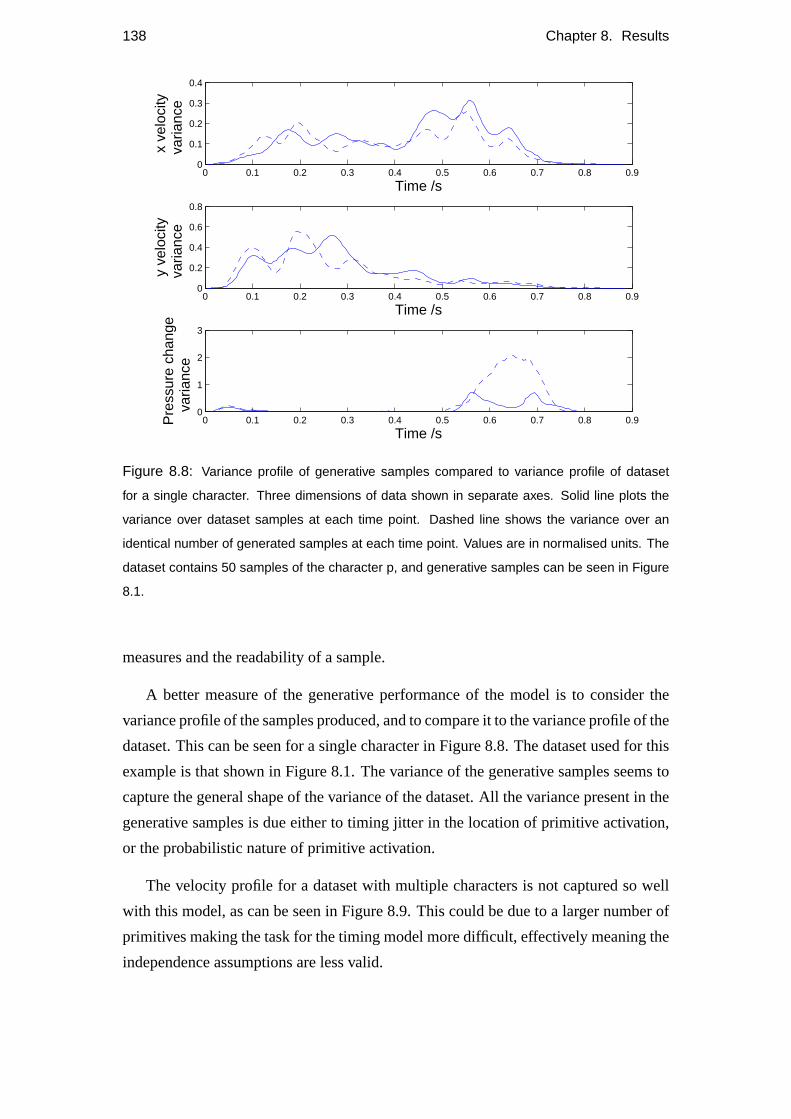
138 Chapter 8. Results
0 0.1 0.2 0.3 0.4 0.5 0.6 0.7 0.8 0.90
0.1
0.2
0.3
0.4
Time /s
x ve
loci
tyva
rianc
e
0 0.1 0.2 0.3 0.4 0.5 0.6 0.7 0.8 0.90
0.2
0.4
0.6
0.8
Time /s
y ve
loci
tyva
rianc
e
0 0.1 0.2 0.3 0.4 0.5 0.6 0.7 0.8 0.90
1
2
3
Time /s
Pre
ssur
e ch
ange
varia
nce
Figure 8.8: Variance profile of generative samples compared to variance profile of dataset
for a single character. Three dimensions of data shown in separate axes. Solid line plots the
variance over dataset samples at each time point. Dashed line shows the variance over an
identical number of generated samples at each time point. Values are in normalised units. The
dataset contains 50 samples of the character p, and generative samples can be seen in Figure
8.1.
measures and the readability of a sample.
A better measure of the generative performance of the model is to consider the
variance profile of the samples produced, and to compare it to the variance profile of the
dataset. This can be seen for a single character in Figure 8.8. The dataset used for this
example is that shown in Figure 8.1. The variance of the generative samples seems to
capture the general shape of the variance of the dataset. All the variance present in the
generative samples is due either to timing jitter in the location of primitive activation,
or the probabilistic nature of primitive activation.
The velocity profile for a dataset with multiple characters is not captured so well
with this model, as can be seen in Figure 8.9. This could be due to a larger number of
primitives making the task for the timing model more difficult, effectively meaning the
independence assumptions are less valid.
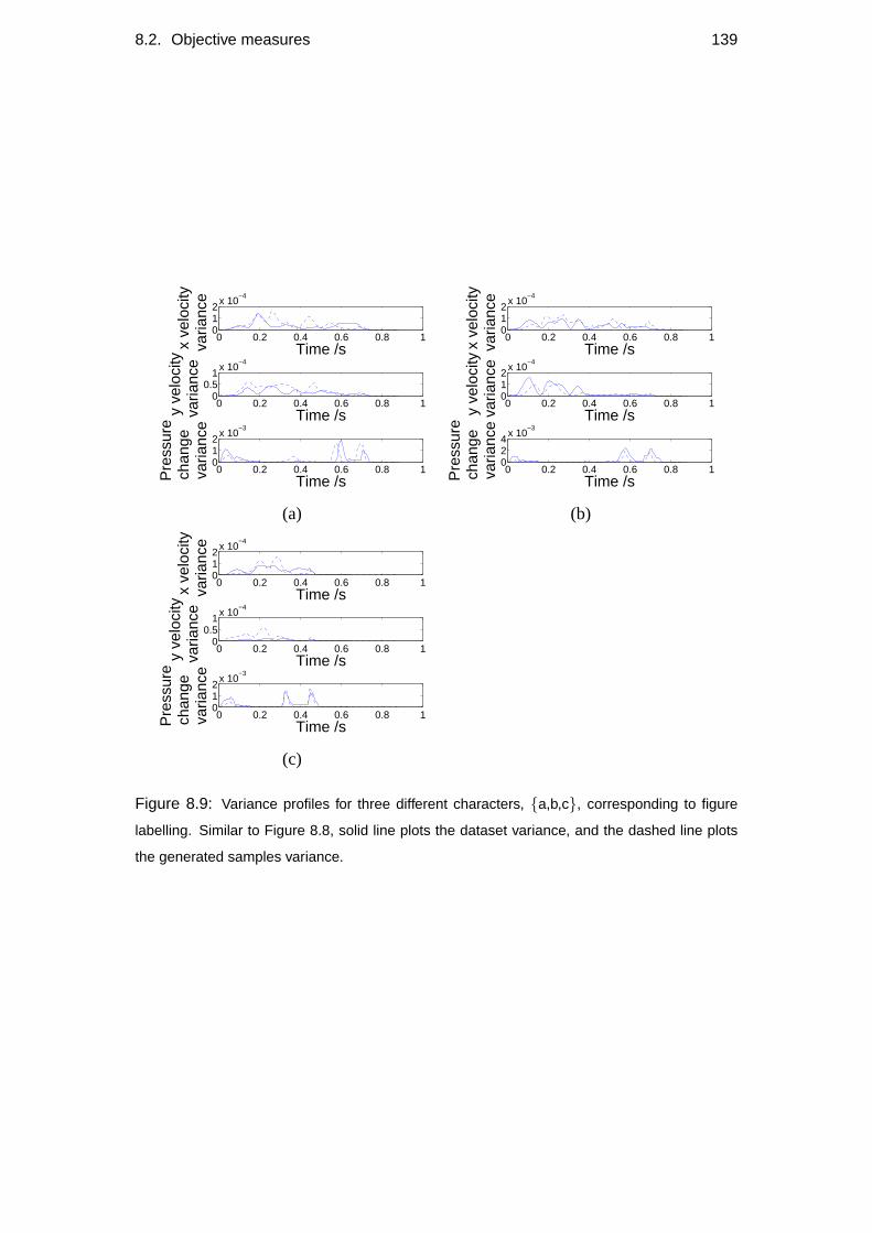
8.2. Objective measures 139
0 0.2 0.4 0.6 0.8 1012
x 10−4
Time /sx ve
loci
tyva
rianc
e
0 0.2 0.4 0.6 0.8 10
0.51
x 10−4
Time /sy ve
loci
tyva
rianc
e
0 0.2 0.4 0.6 0.8 1012
x 10−3
Time /sPre
ssur
ech
ange
va
rianc
e
0 0.2 0.4 0.6 0.8 1012
x 10−4
Time /sx ve
loci
tyva
rianc
e
0 0.2 0.4 0.6 0.8 1012
x 10−4
Time /sy ve
loci
tyva
rianc
e
0 0.2 0.4 0.6 0.8 1024
x 10−3
Time /sPre
ssur
ech
ange
va
rianc
e
(a) (b)
0 0.2 0.4 0.6 0.8 1012
x 10−4
Time /sx ve
loci
tyva
rianc
e
0 0.2 0.4 0.6 0.8 10
0.51
x 10−4
Time /sy ve
loci
tyva
rianc
e
0 0.2 0.4 0.6 0.8 1012
x 10−3
Time /sPre
ssur
ech
ange
va
rianc
e
(c)
Figure 8.9: Variance profiles for three different characters, {a,b,c}, corresponding to figure
labelling. Similar to Figure 8.8, solid line plots the dataset variance, and the dashed line plots
the generated samples variance.
140 Chapter 8. Results
8.3 Primitive swapping
The style of a person’s handwriting is generally something that remains constant over
a long period of time, and is also usually characteristic of the person, despite identical
teaching materials. It is possible that the primitive functions learnt using the model
presented here might capture the style of a person’s handwriting. There are therefore
two distinct forms of variation in handwriting, the variation between character samples
produced from a single writer, and the variation in style across different writers. A
model that distinguishes between these forms of variation would be very useful for
encoding of handwriting. If primitives can capture the style of handwriting of a person
completely, then the timing code of the primitives is effectively a style invariant code
for the characters written. To examine the possibility ofstyle primitives, datasets were
collected from several different writers.1
Normally the coupled model is learnt from a dataset containing multiple character
types from a single writer. In this case, there is a single low level primitive model,
which is shared for all characters, and multiple high level models, with one for each
character. When attempting to compare primitives between writers, we examine a
single character type, but have two separate primitive models. In detail, two datasets
are compared, one from each writer, and two fHMM models are initialised to values
taken from the separate datasets, with the primitive shape initialisations coming from
the mean dataset in corresponding positions. The spike data is concatenated from
both datasets, and a single timing model is learnt from this data. A single spike prior is
produced that couples this timing model with the two primitive models during learning.
The original datasets can be seen in Figure 8.10, showing the difference between
style variation, and the variation present in a single dataset. Training a coupled model
as described above, produces two separate sets of primitives to be learnt, which can be
seen in Figure 8.11.
To examine the inter-changeability of the primitives between sets, the primitives
were progressively swapped from one set to the other, but maintaining the timing in-
formation. This can be seen in Figure 8.12, where each set of axes shows cumulatively
another primitive being swapped to the inappropriate set. This does not result in the
characters becoming unreadable; rather the style of the handwriting gradually changes,
and with all the primitives swapped resembles closely the handwriting style of the sec-
1Thanks to Pooria Zamani of Tehran University for the use of these datasets, which were in factcollected to explore the similarities between Arabic script and Latin script, and whether primitives areshared between the two.
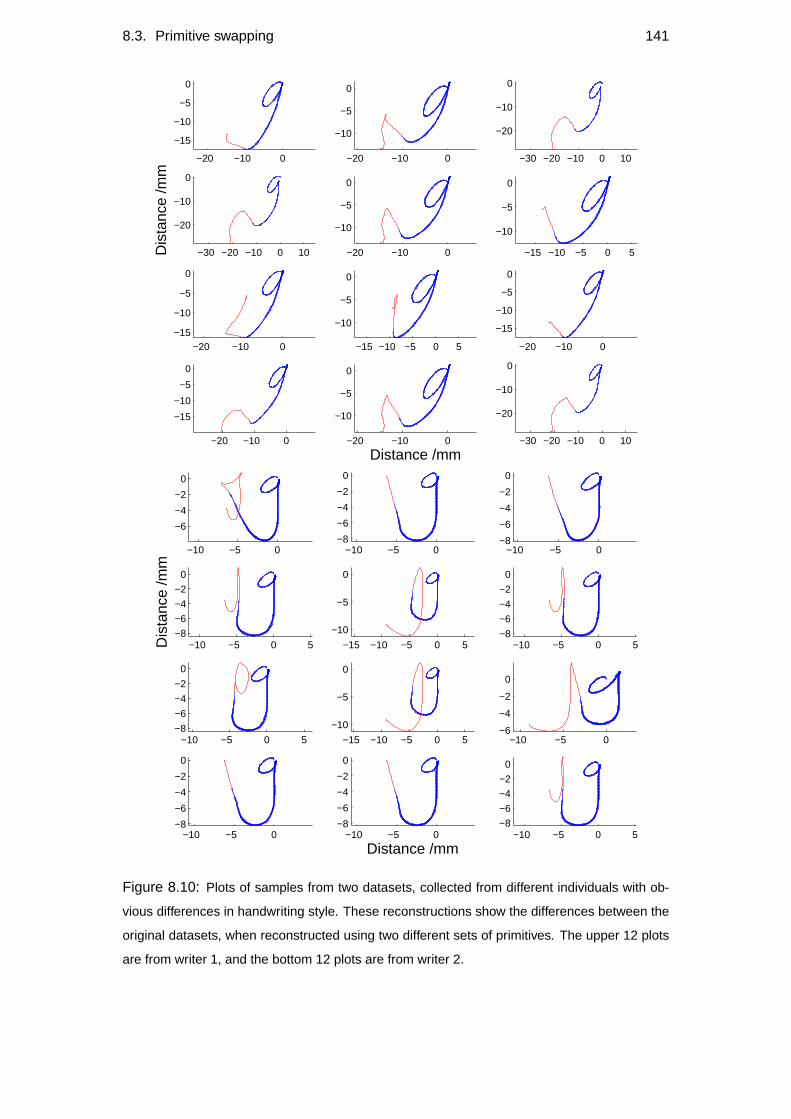
8.3. Primitive swapping 141
−20 −10 0
−15
−10
−5
0
−20 −10 0
−10
−5
0
−30 −20 −10 0 10
−20
−10
0
−30 −20 −10 0 10
−20
−10
0
Dis
tanc
e /m
m
−20 −10 0
−10
−5
0
−15 −10 −5 0 5
−10
−5
0
−20 −10 0−15
−10
−5
0
−15 −10 −5 0 5
−10
−5
0
−20 −10 0
−15
−10
−5
0
−20 −10 0
−15
−10
−5
0
−20 −10 0
−10
−5
0
Distance /mm−30 −20 −10 0 10
−20
−10
0
−10 −5 0
−6
−4
−2
0
−10 −5 0−8
−6
−4
−2
0
−10 −5 0−8
−6
−4
−2
0
−10 −5 0 5−8
−6
−4
−2
0
Dis
tanc
e /m
m
−15 −10 −5 0 5
−10
−5
0
−10 −5 0 5−8
−6
−4
−2
0
−10 −5 0 5−8
−6
−4
−2
0
−15 −10 −5 0 5
−10
−5
0
−10 −5 0−6
−4
−2
0
−10 −5 0−8
−6
−4
−2
0
−10 −5 0−8
−6
−4
−2
0
Distance /mm−10 −5 0 5
−8
−6
−4
−2
0
Figure 8.10: Plots of samples from two datasets, collected from different individuals with ob-
vious differences in handwriting style. These reconstructions show the differences between the
original datasets, when reconstructed using two different sets of primitives. The upper 12 plots
are from writer 1, and the bottom 12 plots are from writer 2.
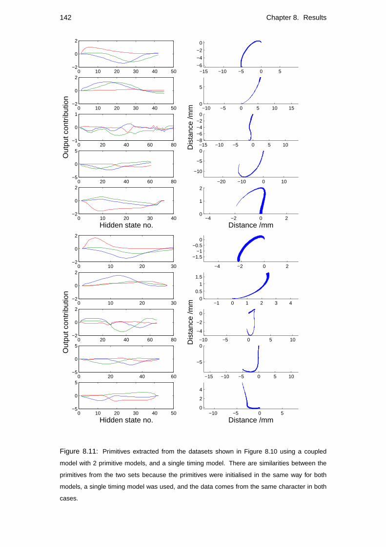
142 Chapter 8. Results
0 10 20 30 40 50−2
0
2
−15 −10 −5 0 5−6
−4
−2
0
0 10 20 30 40 50−2
0
2
−10 −5 0 5 10 150
5
0 20 40 60 80−1
0
1
Out
put c
ontr
ibut
ion
−15 −10 −5 0 5 10−8−6−4−2
0
Dis
tanc
e /m
m0 20 40 60 80
−5
0
5
−20 −10 0 10
−10
−5
0
0 10 20 30 40−2
0
2
Hidden state no.−4 −2 0 2
0
1
2
Distance /mm
0 10 20 30−2
0
2
−4 −2 0 2
−1.5−1
−0.50
0 10 20 30−2
0
2
−1 0 1 2 3 40
0.5
1
1.5
0 20 40 60 80−2
0
2
Out
put c
ontr
ibut
ion
−10 −5 0 5 10
−4
−2
0
Dis
tanc
e /m
m
0 20 40 60−5
0
5
−15 −10 −5 0 5 10
−5
0
0 10 20 30 40 50−5
0
5
Hidden state no.−10 −5 0 5
0
2
4
Distance /mm
Figure 8.11: Primitives extracted from the datasets shown in Figure 8.10 using a coupled
model with 2 primitive models, and a single timing model. There are similarities between the
primitives from the two sets because the primitives were initialised in the same way for both
models, a single timing model was used, and the data comes from the same character in both
cases.
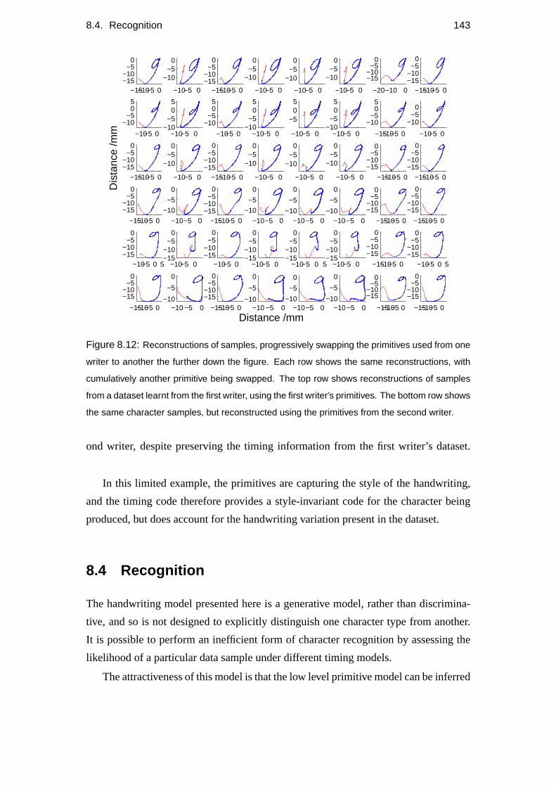
8.4. Recognition 143
−15−10−5 0−15−10
−50
−10−5 0
−10−5
0
−15−10−5 0−15−10
−50
−10−5 0
−10−5
0
−10−5 0
−10−5
0
−10−5 0
−10−5
0
−20−10 0
−15−10
−50
−15−10−5 0−15−10
−50
−10−5 0
−10−5
05
−10−5 0−10
−505
−10−5 0
−10−5
05
−10−5 0−10
−505
−10−5 0
−505
−10−5 0−10
−505
−15−10−5 0
−10−5
05
−10−5 0
−10−5
0
−15−10−5 0
−15−10
−50
Dis
tanc
e /m
m
−10−5 0
−10−5
0
−15−10−5 0−15−10
−50
−10−5 0
−10−5
0
−10−5 0
−10−5
0
−10−5 0
−10−5
0
−15−10−5 0
−15−10
−50
−15−10−5 0−15−10
−50
−15−10−5 0
−15−10
−50
−10−5 0
−10
−5
0
−15−10−5 0−15−10
−50
−10−5 0
−10
−5
0
−10−5 0−10
−5
0
−10−5 0−10
−5
0
−15−10−5 0
−15−10
−50
−15−10−5 0
−15−10
−50
−10−5 0 5−15−10
−50
−10−5 0−15−10
−50
−10−5 0−15−10
−50
−10−5 0−15−10
−50
−10−5 0 5−15−10
−50
−10−5 0−15−10
−50
−15−10−5 0
−15−10
−50
−10−5 0 5−15−10
−50
−15−10−5 0
−15−10
−50
−10 −5 0−10
−5
0
−15−10−5 0
−15−10
−50
−10 −5 0−10
−5
0
Distance /mm−10−5 0
−10
−5
0
−10−5 0−10
−5
0
−15−10−5 0
−15−10
−50
−15−10−5 0
−15−10
−50
Figure 8.12: Reconstructions of samples, progressively swapping the primitives used from one
writer to another the further down the figure. Each row shows the same reconstructions, with
cumulatively another primitive being swapped. The top row shows reconstructions of samples
from a dataset learnt from the first writer, using the first writer’s primitives. The bottom row shows
the same character samples, but reconstructed using the primitives from the second writer.
ond writer, despite preserving the timing information from the first writer’s dataset.
In this limited example, the primitives are capturing the style of the handwriting,
and the timing code therefore provides a style-invariant code for the character being
produced, but does account for the handwriting variation present in the dataset.
8.4 Recognition
The handwriting model presented here is a generative model, rather than discrimina-
tive, and so is not designed to explicitly distinguish one character type from another.
It is possible to perform an inefficient form of character recognition by assessing the
likelihood of a particular data sample under different timing models.
The attractiveness of this model is that the low level primitive model can be inferred
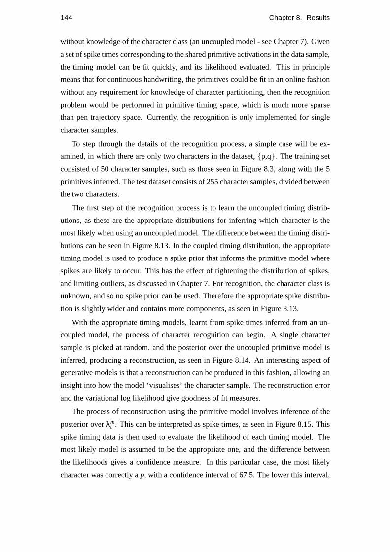
144 Chapter 8. Results
without knowledge of the character class (an uncoupled model - see Chapter 7). Given
a set of spike times corresponding to the shared primitive activations in the data sample,
the timing model can be fit quickly, and its likelihood evaluated. This in principle
means that for continuous handwriting, the primitives could be fit in an online fashion
without any requirement for knowledge of character partitioning, then the recognition
problem would be performed in primitive timing space, which is much more sparse
than pen trajectory space. Currently, the recognition is only implemented for single
character samples.
To step through the details of the recognition process, a simple case will be ex-
amined, in which there are only two characters in the dataset,{p,q}. The training set
consisted of 50 character samples, such as those seen in Figure 8.3, along with the 5
primitives inferred. The test dataset consists of 255 character samples, divided between
the two characters.
The first step of the recognition process is to learn the uncoupled timing distrib-
utions, as these are the appropriate distributions for inferring which character is the
most likely when using an uncoupled model. The difference between the timing distri-
butions can be seen in Figure 8.13. In the coupled timing distribution, the appropriate
timing model is used to produce a spike prior that informs the primitive model where
spikes are likely to occur. This has the effect of tightening the distribution of spikes,
and limiting outliers, as discussed in Chapter 7. For recognition, the character class is
unknown, and so no spike prior can be used. Therefore the appropriate spike distribu-
tion is slightly wider and contains more components, as seen in Figure 8.13.
With the appropriate timing models, learnt from spike times inferred from an un-
coupled model, the process of character recognition can begin. A single character
sample is picked at random, and the posterior over the uncoupled primitive model is
inferred, producing a reconstruction, as seen in Figure 8.14. An interesting aspect of
generative models is that a reconstruction can be produced in this fashion, allowing an
insight into how the model ‘visualises’ the character sample. The reconstruction error
and the variational log likelihood give goodness of fit measures.
The process of reconstruction using the primitive model involves inference of the
posterior overλmt . This can be interpreted as spike times, as seen in Figure 8.15. This
spike timing data is then used to evaluate the likelihood of each timing model. The
most likely model is assumed to be the appropriate one, and the difference between
the likelihoods gives a confidence measure. In this particular case, the most likely
character was correctly ap, with a confidence interval of 67.5. The lower this interval,
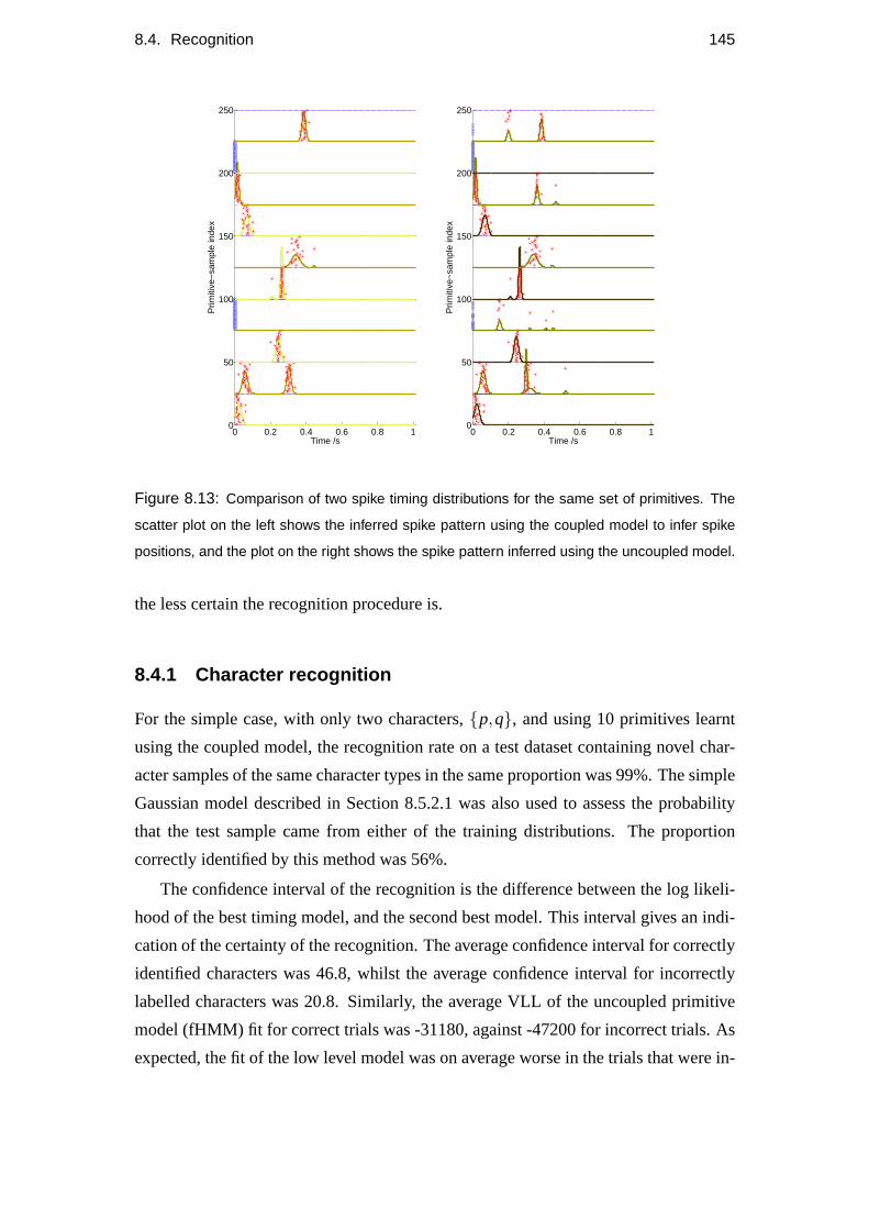
8.4. Recognition 145
0 0.2 0.4 0.6 0.8 10
50
100
150
200
250
Time /s
Prim
itive
−sa
mpl
e in
dex
0 0.2 0.4 0.6 0.8 10
50
100
150
200
250
Time /sP
rimiti
ve−
sam
ple
inde
x
Figure 8.13: Comparison of two spike timing distributions for the same set of primitives. The
scatter plot on the left shows the inferred spike pattern using the coupled model to infer spike
positions, and the plot on the right shows the spike pattern inferred using the uncoupled model.
the less certain the recognition procedure is.
8.4.1 Character recognition
For the simple case, with only two characters,{p,q}, and using 10 primitives learnt
using the coupled model, the recognition rate on a test dataset containing novel char-
acter samples of the same character types in the same proportion was 99%. The simple
Gaussian model described in Section 8.5.2.1 was also used to assess the probability
that the test sample came from either of the training distributions. The proportion
correctly identified by this method was 56%.
The confidence interval of the recognition is the difference between the log likeli-
hood of the best timing model, and the second best model. This interval gives an indi-
cation of the certainty of the recognition. The average confidence interval for correctly
identified characters was 46.8, whilst the average confidence interval for incorrectly
labelled characters was 20.8. Similarly, the average VLL of the uncoupled primitive
model (fHMM) fit for correct trials was -31180, against -47200 for incorrect trials. As
expected, the fit of the low level model was on average worse in the trials that were in-
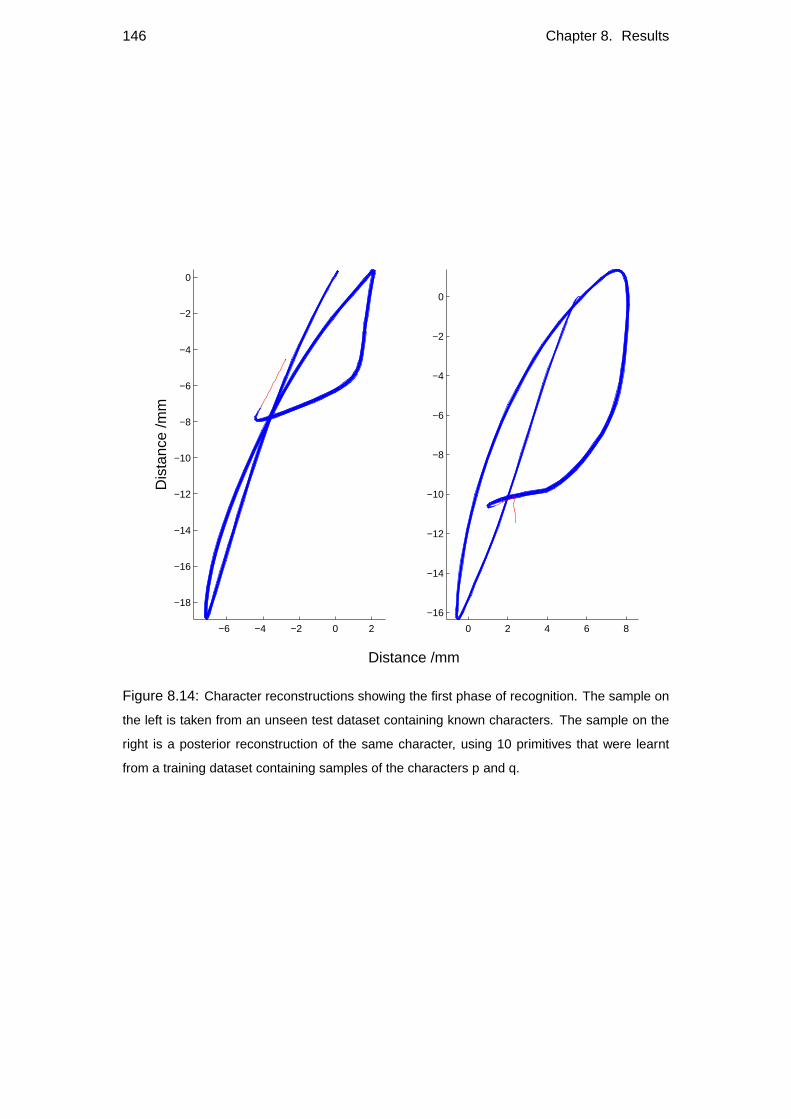
146 Chapter 8. Results
−6 −4 −2 0 2
−18
−16
−14
−12
−10
−8
−6
−4
−2
0
Distance /mm
Dis
tanc
e /m
m
0 2 4 6 8
−16
−14
−12
−10
−8
−6
−4
−2
0
Figure 8.14: Character reconstructions showing the first phase of recognition. The sample on
the left is taken from an unseen test dataset containing known characters. The sample on the
right is a posterior reconstruction of the same character, using 10 primitives that were learnt
from a training dataset containing samples of the characters p and q.
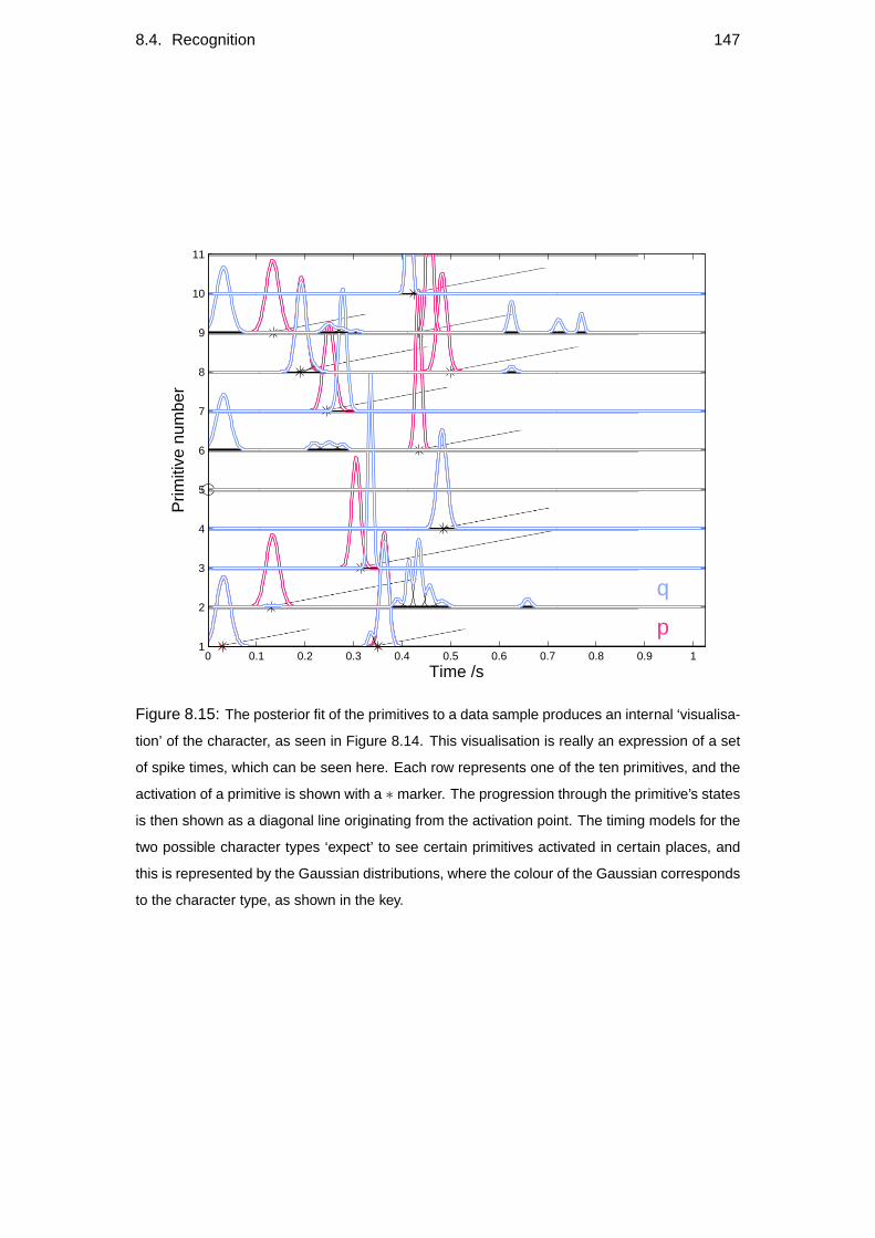
8.4. Recognition 147
Time /s
Prim
itive
num
ber
p
q
0 0.1 0.2 0.3 0.4 0.5 0.6 0.7 0.8 0.9 11
2
3
4
5
6
7
8
9
10
11
Figure 8.15: The posterior fit of the primitives to a data sample produces an internal ‘visualisa-
tion’ of the character, as seen in Figure 8.14. This visualisation is really an expression of a set
of spike times, which can be seen here. Each row represents one of the ten primitives, and the
activation of a primitive is shown with a ∗ marker. The progression through the primitive’s states
is then shown as a diagonal line originating from the activation point. The timing models for the
two possible character types ‘expect’ to see certain primitives activated in certain places, and
this is represented by the Gaussian distributions, where the colour of the Gaussian corresponds
to the character type, as shown in the key.
148 Chapter 8. Results
correctly identified, and likewise the difference in the likelihood between the possible
timing models was smaller on incorrect trials.
On a larger dataset, containing several characters, the recognition performance de-
creases, as the timing model becomes inadequate at modelling the variance in the data.
A better timing model, with more dependencies between the presence of components
would help with more generalised recognition performance.
The drawback with using the fHMM for character recognition is that the inference
of the posterior takes a significant time. For a single character it took on average 13
seconds to perform the recognition, including fHMM and multiple HMM posterior in-
ference. A greedy initialisation of the fHMM states might improve the performance. A
convolution function provides one quick approach to this problem, and a similar model
is discussed and compared in Section 8.5.2.3 which uses such a technique. Potentially
a combination of the two approaches could provide a solution to the speed problem.
Alternatively, approximate inference, or semi-convergence could be explored for speed
improvement. Additionally, the factorial nature of the fHMM would lend itself towards
parallelization, which would improve the performance further.
8.5 Comparison with other models
Several primitive based models were discussed in Chapter 2. Some models consider
primitives to be time-slice components, rather than time extended blocks. In this sec-
tion we look at some related models, and compare the performance of these models
with the primitive based model presented earlier.
8.5.1 Objective measures
8.5.1.1 TAMPE and TASDPE
Model performance can be assessed in different ways; however the most common
model independent assessment compares the reconstructed samples to the original
ones, calculating the reconstruction error. For generative models, this cannot be done
as there are no exact original samples to compare with. A similar assessment for gener-
ative samples is to look at the statistics of the generative data, over many samples. The
mean and the variance over all the samples can then be compared to the mean and vari-
ance of the original dataset, or a test dataset, at each time point. These measures create
error profiles for the character, the absolute sums of which provide objective measures
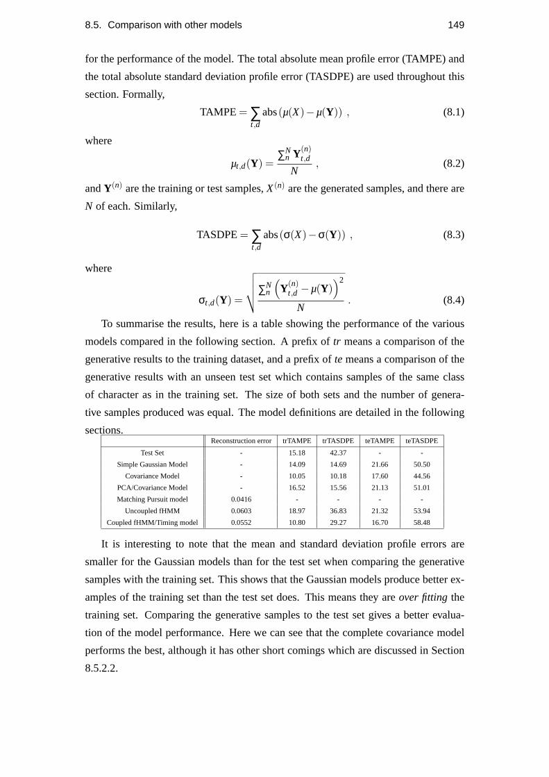
8.5. Comparison with other models 149
for the performance of the model. The total absolute mean profile error (TAMPE) and
the total absolute standard deviation profile error (TASDPE) are used throughout this
section. Formally,
TAMPE = ∑t,d
abs(µ(X)−µ(Y)) , (8.1)
where
µt,d(Y) =∑N
n Y(n)t,d
N, (8.2)
andY(n) are the training or test samples,X(n) are the generated samples, and there are
N of each. Similarly,
TASDPE= ∑t,d
abs(σ(X)−σ(Y)) , (8.3)
where
σt,d(Y) =
√√√√∑Nn
(Y(n)
t,d −µ(Y))2
N. (8.4)
To summarise the results, here is a table showing the performance of the various
models compared in the following section. A prefix oftr means a comparison of the
generative results to the training dataset, and a prefix ofte means a comparison of the
generative results with an unseen test set which contains samples of the same class
of character as in the training set. The size of both sets and the number of genera-
tive samples produced was equal. The model definitions are detailed in the following
sections.Reconstruction error trTAMPE trTASDPE teTAMPE teTASDPE
Test Set - 15.18 42.37 - -
Simple Gaussian Model - 14.09 14.69 21.66 50.50
Covariance Model - 10.05 10.18 17.60 44.56
PCA/Covariance Model - 16.52 15.56 21.13 51.01
Matching Pursuit model 0.0416 - - - -
Uncoupled fHMM 0.0603 18.97 36.83 21.32 53.94
Coupled fHMM/Timing model 0.0552 10.80 29.27 16.70 58.48
It is interesting to note that the mean and standard deviation profile errors are
smaller for the Gaussian models than for the test set when comparing the generative
samples with the training set. This shows that the Gaussian models produce better ex-
amples of the training set than the test set does. This means they areover fitting the
training set. Comparing the generative samples to the test set gives a better evalua-
tion of the model performance. Here we can see that the complete covariance model
performs the best, although it has other short comings which are discussed in Section
8.5.2.2.
150 Chapter 8. Results
The reconstruction error for the Matching Pursuit/Gradient descent algorithm was
smaller than for the fHMM based model, due to the possibility of using a scaling factor.
In this case, 10 atomic functions were used and 650 occurrences of atoms were fit to
the data, equalling on average, one of each atom per character. Although the number
of occurrences of the primitives in the fHMM based model are not constrained, the
MAP number of spikes was of the same order as this. Without a generalising model
across the character samples, the Matching Pursuit algorithm is not generative, and so
the TAMPE and TASDPE measures are not calculable. (They could be calculated on
the reconstructed dataset, and as such would seem to strongly over-fit the data.)
The performance of the uncoupled and coupled models was very similar by these
measures, and they are both comparable to the PCA/Covariance model, where 10 PCA
components were used. The main advantage of the fHMM primitive based model is
that the same primitives (or components) can be used to model parts of other characters,
whereas the covariance based models do not allow offsets, and so the components are
only going to be suitable for a single type of character, or very similar ones such as ab
and anh.
The coupled model performed slightly better than the uncoupled model, producing
samples that were closer to the mean character sample from both the training set and
the test set.
8.5.2 Alternative models
8.5.2.1 Simple Gaussian model
A straightforward model of a character is to assume that the data is independent at each
time point, and modelled by a Gaussian distribution.
P(Y) = ∏t
N (µµµt ,σt) , (8.5)
whereµµµt andσt are learnt using standard estimators.
This distribution is parameterised by taking the mean and variance of the character
samples. Sampling from such a model produces generative characters as seen in Figure
8.16.
The wobbly nature of the samples produced by this model is due to the indepen-
dence assumption implicit in the model, meaning that the samples at adjacent time
points are independent. The shape of the samples in general however is reasonably
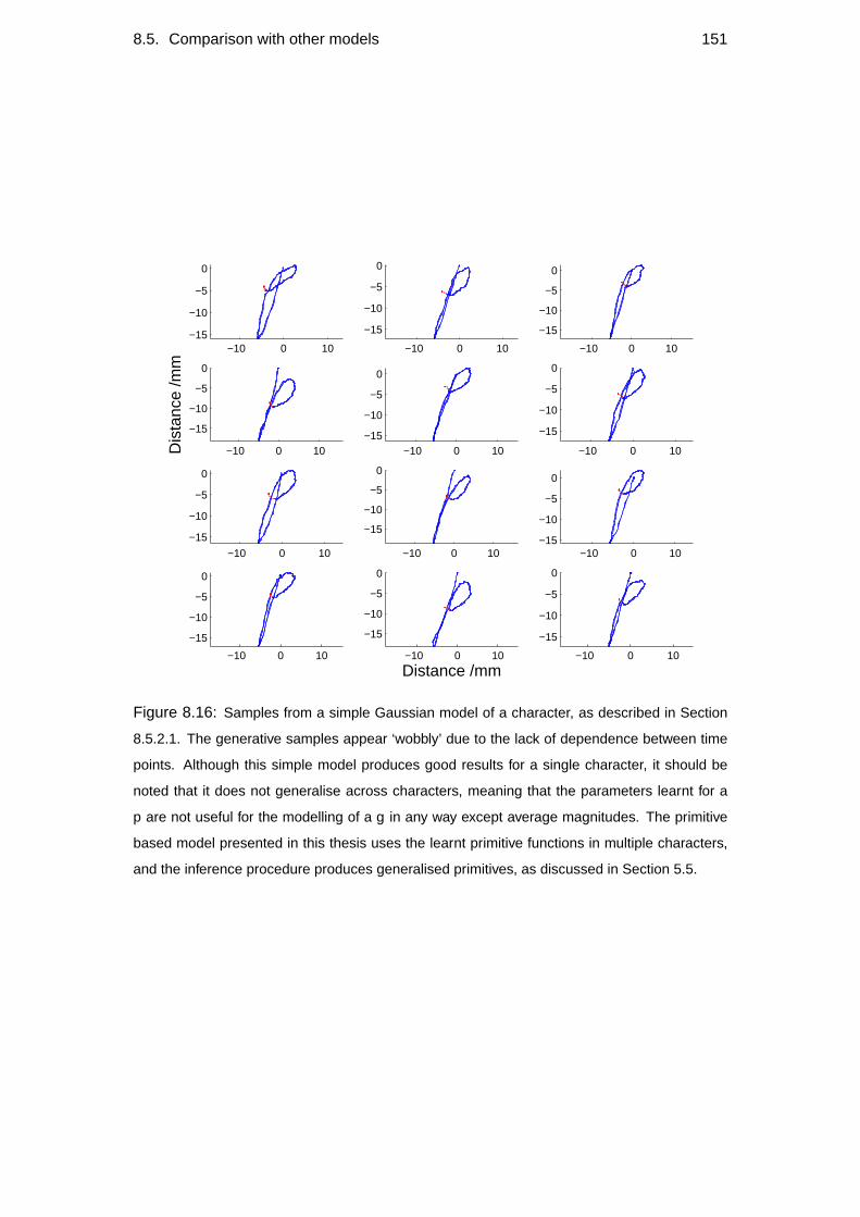
8.5. Comparison with other models 151
−10 0 10−15
−10
−5
0
−10 0 10
−15
−10
−5
0
−10 0 10
−15
−10
−5
0
−10 0 10
−15
−10
−5
0
Dis
tanc
e /m
m
−10 0 10−15
−10
−5
0
−10 0 10
−15
−10
−5
0
−10 0 10
−15
−10
−5
0
−10 0 10
−15
−10
−5
0
−10 0 10−15
−10
−5
0
−10 0 10
−15
−10
−5
0
−10 0 10
−15
−10
−5
0
Distance /mm−10 0 10
−15
−10
−5
0
Figure 8.16: Samples from a simple Gaussian model of a character, as described in Section
8.5.2.1. The generative samples appear ‘wobbly’ due to the lack of dependence between time
points. Although this simple model produces good results for a single character, it should be
noted that it does not generalise across characters, meaning that the parameters learnt for a
p are not useful for the modelling of a g in any way except average magnitudes. The primitive
based model presented in this thesis uses the learnt primitive functions in multiple characters,
and the inference procedure produces generalised primitives, as discussed in Section 5.5.
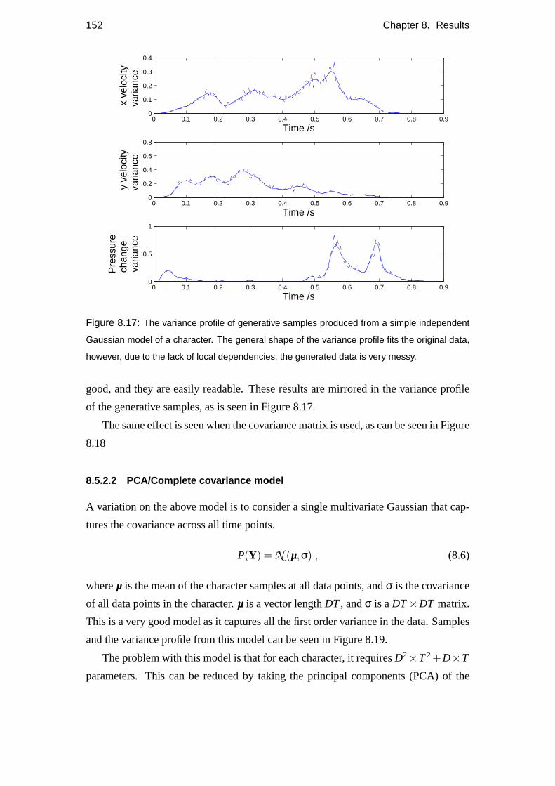
152 Chapter 8. Results
0 0.1 0.2 0.3 0.4 0.5 0.6 0.7 0.8 0.90
0.1
0.2
0.3
0.4
Time /sx
velo
city
varia
nce
0 0.1 0.2 0.3 0.4 0.5 0.6 0.7 0.8 0.90
0.2
0.4
0.6
0.8
Time /s
y ve
loci
tyva
rianc
e
0 0.1 0.2 0.3 0.4 0.5 0.6 0.7 0.8 0.90
0.5
1
Time /s
Pre
ssur
ech
ange
va
rianc
e
Figure 8.17: The variance profile of generative samples produced from a simple independent
Gaussian model of a character. The general shape of the variance profile fits the original data,
however, due to the lack of local dependencies, the generated data is very messy.
good, and they are easily readable. These results are mirrored in the variance profile
of the generative samples, as is seen in Figure 8.17.
The same effect is seen when the covariance matrix is used, as can be seen in Figure
8.18
8.5.2.2 PCA/Complete covariance model
A variation on the above model is to consider a single multivariate Gaussian that cap-
tures the covariance across all time points.
P(Y) = N (µµµ,σ) , (8.6)
whereµµµ is the mean of the character samples at all data points, andσ is the covariance
of all data points in the character.µµµ is a vector lengthDT, andσ is aDT×DT matrix.
This is a very good model as it captures all the first order variance in the data. Samples
and the variance profile from this model can be seen in Figure 8.19.
The problem with this model is that for each character, it requiresD2×T2+D×T
parameters. This can be reduced by taking the principal components (PCA) of the
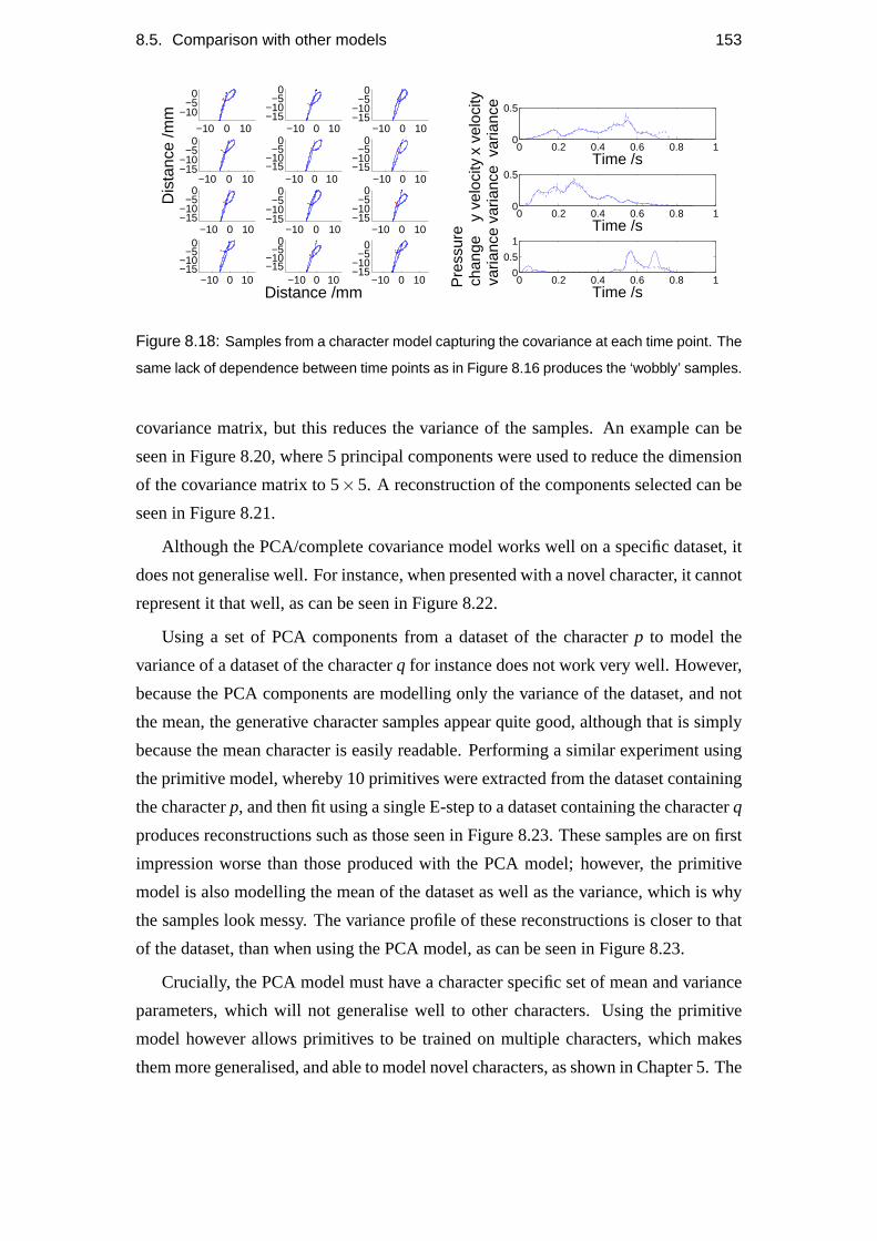
8.5. Comparison with other models 153
−10 0 10
−10−5
0
−10 0 10−15−10
−50
−10 0 10−15−10
−50
−10 0 10−15−10
−50
Dis
tanc
e /m
m−10 0 10
−15−10
−50
−10 0 10−15−10
−50
−10 0 10−15−10
−50
−10 0 10−15−10
−50
−10 0 10−15−10
−50
−10 0 10−15−10
−50
−10 0 10−15−10
−50
Distance /mm−10 0 10
−15−10
−50
0 0.2 0.4 0.6 0.8 10
0.5
Time /s
x ve
loci
tyva
rianc
e
0 0.2 0.4 0.6 0.8 10
0.5
Time /s
y ve
loci
tyva
rianc
e
0 0.2 0.4 0.6 0.8 10
0.5
1
Time /s
Pre
ssur
ech
ange
va
rianc
e
Figure 8.18: Samples from a character model capturing the covariance at each time point. The
same lack of dependence between time points as in Figure 8.16 produces the ‘wobbly’ samples.
covariance matrix, but this reduces the variance of the samples. An example can be
seen in Figure 8.20, where 5 principal components were used to reduce the dimension
of the covariance matrix to 5×5. A reconstruction of the components selected can be
seen in Figure 8.21.
Although the PCA/complete covariance model works well on a specific dataset, it
does not generalise well. For instance, when presented with a novel character, it cannot
represent it that well, as can be seen in Figure 8.22.
Using a set of PCA components from a dataset of the characterp to model the
variance of a dataset of the characterq for instance does not work very well. However,
because the PCA components are modelling only the variance of the dataset, and not
the mean, the generative character samples appear quite good, although that is simply
because the mean character is easily readable. Performing a similar experiment using
the primitive model, whereby 10 primitives were extracted from the dataset containing
the characterp, and then fit using a single E-step to a dataset containing the characterq
produces reconstructions such as those seen in Figure 8.23. These samples are on first
impression worse than those produced with the PCA model; however, the primitive
model is also modelling the mean of the dataset as well as the variance, which is why
the samples look messy. The variance profile of these reconstructions is closer to that
of the dataset, than when using the PCA model, as can be seen in Figure 8.23.
Crucially, the PCA model must have a character specific set of mean and variance
parameters, which will not generalise well to other characters. Using the primitive
model however allows primitives to be trained on multiple characters, which makes
them more generalised, and able to model novel characters, as shown in Chapter 5. The
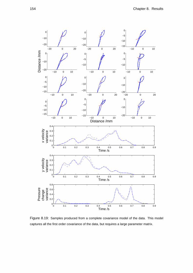
154 Chapter 8. Results
−20 0 20
−20
−10
0
−20 0 20
−20
−10
0
−10 0 10−15
−10
−5
0
−10 0 10−20
−10
0
Dis
tanc
e /m
m
−10 0 10
−10
−5
0
−10 0 10
−10
−5
0
−10 0 10−15
−10
−5
0
−20 0 20
−20
−10
0
−20 0 20−20
−10
0
−10 0 10
−15
−10
−5
0
−10 0 10−15
−10
−5
0
Distance /mm−10 0 10
−20
−10
0
0 0.1 0.2 0.3 0.4 0.5 0.6 0.7 0.8 0.90
0.1
0.2
0.3
0.4
Time /s
x ve
loci
tyva
rianc
e
0 0.1 0.2 0.3 0.4 0.5 0.6 0.7 0.8 0.90
0.1
0.2
0.3
0.4
Time /s
y ve
loci
tyva
rianc
e
0 0.1 0.2 0.3 0.4 0.5 0.6 0.7 0.8 0.90
0.2
0.4
0.6
0.8
Time /s
Pre
ssur
ech
ange
va
rianc
e
Figure 8.19: Samples produced from a complete covariance model of the data. This model
captures all the first order covariance of the data, but requires a large parameter matrix.

8.5. Comparison with other models 155
−10 0 10−15
−10
−5
0
−20 −10 0 10
−15
−10
−5
0
−20 −10 0 10
−20
−10
0
−10 0 10−15
−10
−5
0
Dis
tanc
e /m
m
−10 0 10
−15
−10
−5
0
−10 0 10−15
−10
−5
0
−10 0 10
−15
−10
−5
0
−10 0 10−15
−10
−5
0
−10 0 10
−10
−5
0
−10 0 10
−15
−10
−5
0
−10 0 10−15
−10
−5
0
Distance /mm−20 0 20
−20
−10
0
0 0.1 0.2 0.3 0.4 0.5 0.6 0.7 0.8 0.90
0.1
0.2
0.3
0.4
Time /s
x ve
loci
tyva
rianc
e
0 0.1 0.2 0.3 0.4 0.5 0.6 0.7 0.8 0.90
0.1
0.2
0.3
0.4
Time /s
y ve
loci
tyva
rianc
e
0 0.1 0.2 0.3 0.4 0.5 0.6 0.7 0.8 0.90
0.2
0.4
0.6
0.8
Time /s
Pre
ssur
ech
ange
va
rianc
e
Figure 8.20: Samples produced using the complete covariance model described in Section
8.5.2.2, but using PCA to reduce the dimension of the covariance matrix to 5×5. This reduces
the number of parameters needed, but also reduces the variance of the samples produced, as
can be seen in the variance profile plots. A reconstruction of the principal components selected
using PCA can be seen in Figure 8.21.
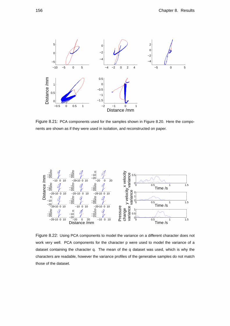
156 Chapter 8. Results
−10 −5 0 5
−5
0
5
−4 −2 0 2 4
−4
−2
0
−5 0 5
−4
−2
0
2
−0.5 0 0.5 1
0
0.5
1
Dis
tanc
e /m
m
−2 −1 0 1
−1.5
−1
−0.5
0
0.5
Distance /mm
Figure 8.21: PCA components used for the samples shown in Figure 8.20. Here the compo-
nents are shown as if they were used in isolation, and reconstructed on paper.
−10 0 10−15−10
−50
−20−10 0 10−15−10
−50
−20 0 20−20−10
0
−20−10 0 10−15−10
−50
Dis
tanc
e /m
m
−20−10 0 10−15−10
−50
−20−10 0 10−15−10
−50
−20−10 0 10−20−10
0
−10 0 10−15−10
−50
−20−10 0 10−15−10
−50
−20−10 0 10−15−10
−50
−20 0 20−20−10
0
Distance /mm−10 0 10
−15−10
−50
0 0.5 1 1.50
0.5
Time /s
x ve
loci
tyva
rianc
e
0 0.5 1 1.50
1
2
Time /s
y ve
loci
tyva
rianc
e
0 0.5 1 1.50
0.5
1
Time /s
Pre
ssur
ech
ange
va
rianc
e
Figure 8.22: Using PCA components to model the variance on a different character does not
work very well. PCA components for the character p were used to model the variance of a
dataset containing the character q. The mean of the q dataset was used, which is why the
characters are readable, however the variance profiles of the generative samples do not match
those of the dataset.
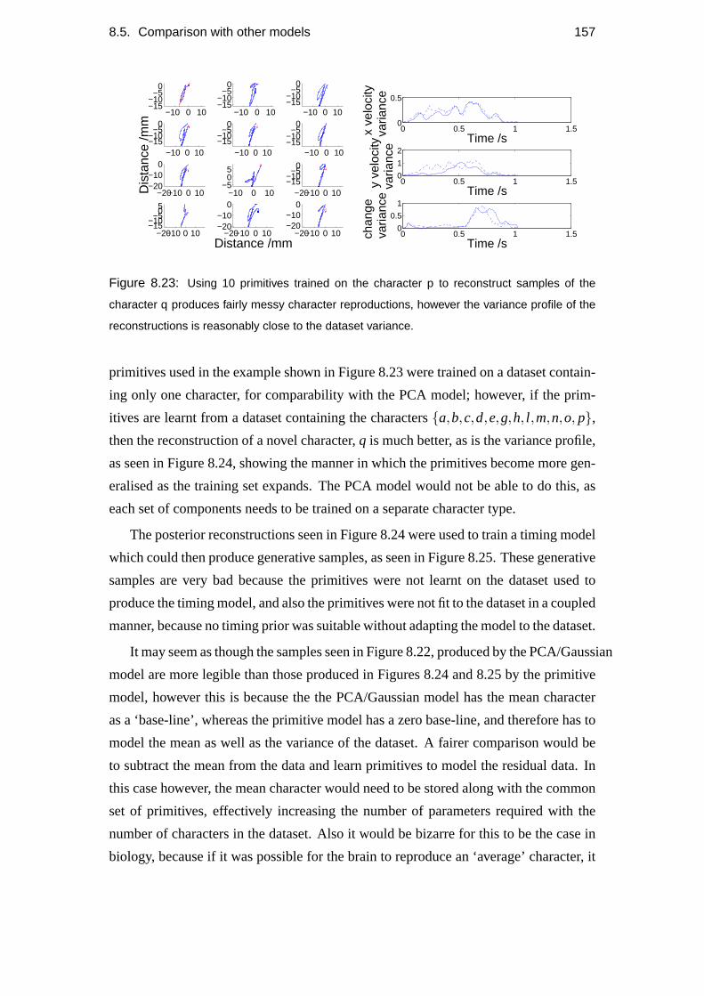
8.5. Comparison with other models 157
−10 0 10−15−10
−50
−10 0 10−15−10
−50
−10 0 10−15−10
−50
−10 0 10−15−10
−50
Dis
tanc
e /m
m−10 0 10
−15−10
−50
−10 0 10−15−10
−50
−20−10 0 10−20−10
0
−10 0 10−5
05
−20−10 0 10−15−10
−50
−20−10 0 10−15−10−50
5
−20−10 0 10−20−10
0
Distance /mm−20−10 0 10
−20−10
0
0 0.5 1 1.50
0.5
Time /sx ve
loci
tyva
rianc
e
0 0.5 1 1.50
1
2
Time /sy ve
loci
tyva
rianc
e
0 0.5 1 1.50
0.5
1
Time /s
Pre
ssur
ech
ange
va
rianc
e
Figure 8.23: Using 10 primitives trained on the character p to reconstruct samples of the
character q produces fairly messy character reproductions, however the variance profile of the
reconstructions is reasonably close to the dataset variance.
primitives used in the example shown in Figure 8.23 were trained on a dataset contain-
ing only one character, for comparability with the PCA model; however, if the prim-
itives are learnt from a dataset containing the characters{a,b,c,d,e,g,h, l ,m,n,o, p},then the reconstruction of a novel character,q is much better, as is the variance profile,
as seen in Figure 8.24, showing the manner in which the primitives become more gen-
eralised as the training set expands. The PCA model would not be able to do this, as
each set of components needs to be trained on a separate character type.
The posterior reconstructions seen in Figure 8.24 were used to train a timing model
which could then produce generative samples, as seen in Figure 8.25. These generative
samples are very bad because the primitives were not learnt on the dataset used to
produce the timing model, and also the primitives were not fit to the dataset in a coupled
manner, because no timing prior was suitable without adapting the model to the dataset.
It may seem as though the samples seen in Figure 8.22, produced by the PCA/Gaussian
model are more legible than those produced in Figures 8.24 and 8.25 by the primitive
model, however this is because the the PCA/Gaussian model has the mean character
as a ‘base-line’, whereas the primitive model has a zero base-line, and therefore has to
model the mean as well as the variance of the dataset. A fairer comparison would be
to subtract the mean from the data and learn primitives to model the residual data. In
this case however, the mean character would need to be stored along with the common
set of primitives, effectively increasing the number of parameters required with the
number of characters in the dataset. Also it would be bizarre for this to be the case in
biology, because if it was possible for the brain to reproduce an ‘average’ character, it
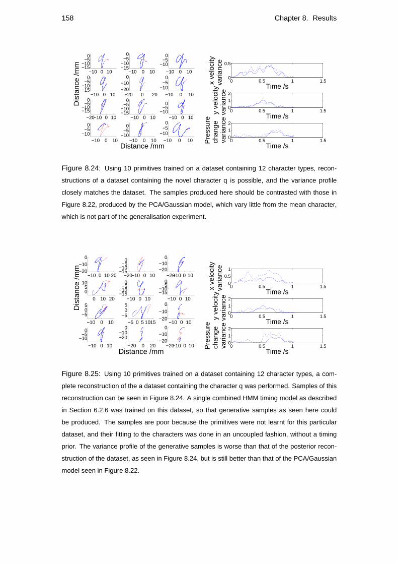
158 Chapter 8. Results
−10 0 10−15−10
−50
−10 0 10−15−10
−50
−10 0 10
−10−5
0
−10 0 10−15−10
−50
Dis
tanc
e /m
m
−20 0 20−20−10
0
−10 0 10−10
−50
−20−10 0 10−15−10
−50
−10 0 10−15−10
−50
−10 0 10−10
−50
−10 0 10−10
−50
−10 0 10−10
−50
Distance /mm−10 0 10
−10−5
0
0 0.5 1 1.50
0.5
Time /s
x ve
loci
tyva
rianc
e
0 0.5 1 1.50
1
2
Time /s
y ve
loci
tyva
rianc
e
0 0.5 1 1.50
1
2
Time /s
Pre
ssur
ech
ange
va
rianc
e
Figure 8.24: Using 10 primitives trained on a dataset containing 12 character types, recon-
structions of a dataset containing the novel character q is possible, and the variance profile
closely matches the dataset. The samples produced here should be contrasted with those in
Figure 8.22, produced by the PCA/Gaussian model, which vary little from the mean character,
which is not part of the generalisation experiment.
−10 0 10 20−20−10
0
−20−10 0 10−15−10
−50
−20−10 0 10−20−10
0
0 10 20
05
10
Dis
tanc
e /m
m
−10 0 10−15−10
−50
−10 0 10−15−10
−50
−10 0 10
−505
−5 0 5 1015−5
05
−10 0 10−20
−10
0
−10 0 10
−10−5
0
−20 0 20
−20−10
0
Distance /mm−20−10 0 10
−20−10
0
0 0.5 1 1.50
0.5
1
Time /s
x ve
loci
tyva
rianc
e
0 0.5 1 1.50
1
2
Time /s
y ve
loci
tyva
rianc
e
0 0.5 1 1.50
1
2
Time /s
Pre
ssur
ech
ange
va
rianc
e
Figure 8.25: Using 10 primitives trained on a dataset containing 12 character types, a com-
plete reconstruction of the a dataset containing the character q was performed. Samples of this
reconstruction can be seen in Figure 8.24. A single combined HMM timing model as described
in Section 6.2.6 was trained on this dataset, so that generative samples as seen here could
be produced. The samples are poor because the primitives were not learnt for this particular
dataset, and their fitting to the characters was done in an uncoupled fashion, without a timing
prior. The variance profile of the generative samples is worse than that of the posterior recon-
struction of the dataset, as seen in Figure 8.24, but is still better than that of the PCA/Gaussian
model seen in Figure 8.22.
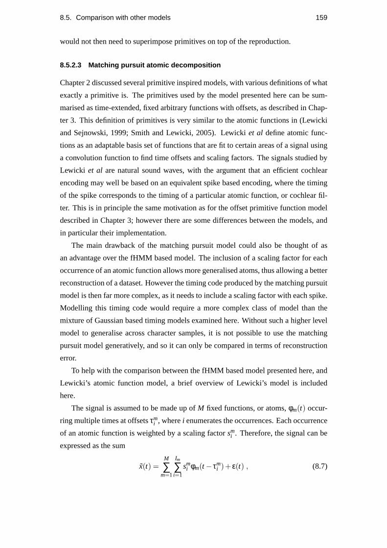
8.5. Comparison with other models 159
would not then need to superimpose primitives on top of the reproduction.
8.5.2.3 Matching pursuit atomic decomposition
Chapter 2 discussed several primitive inspired models, with various definitions of what
exactly a primitive is. The primitives used by the model presented here can be sum-
marised as time-extended, fixed arbitrary functions with offsets, as described in Chap-
ter 3. This definition of primitives is very similar to the atomic functions in (Lewicki
and Sejnowski, 1999; Smith and Lewicki, 2005). Lewickiet al define atomic func-
tions as an adaptable basis set of functions that are fit to certain areas of a signal using
a convolution function to find time offsets and scaling factors. The signals studied by
Lewicki et al are natural sound waves, with the argument that an efficient cochlear
encoding may well be based on an equivalent spike based encoding, where the timing
of the spike corresponds to the timing of a particular atomic function, or cochlear fil-
ter. This is in principle the same motivation as for the offset primitive function model
described in Chapter 3; however there are some differences between the models, and
in particular their implementation.
The main drawback of the matching pursuit model could also be thought of as
an advantage over the fHMM based model. The inclusion of a scaling factor for each
occurrence of an atomic function allows more generalised atoms, thus allowing a better
reconstruction of a dataset. However the timing code produced by the matching pursuit
model is then far more complex, as it needs to include a scaling factor with each spike.
Modelling this timing code would require a more complex class of model than the
mixture of Gaussian based timing models examined here. Without such a higher level
model to generalise across character samples, it is not possible to use the matching
pursuit model generatively, and so it can only be compared in terms of reconstruction
error.
To help with the comparison between the fHMM based model presented here, and
Lewicki’s atomic function model, a brief overview of Lewicki’s model is included
here.
The signal is assumed to be made up ofM fixed functions, or atoms,φm(t) occur-
ring multiple times at offsetsτmi , wherei enumerates the occurrences. Each occurrence
of an atomic function is weighted by a scaling factorsmi . Therefore, the signal can be
expressed as the sum
x(t) =M
∑m=1
Im
∑i=1
smi φm(t− τm
i )+ ε(t) , (8.7)
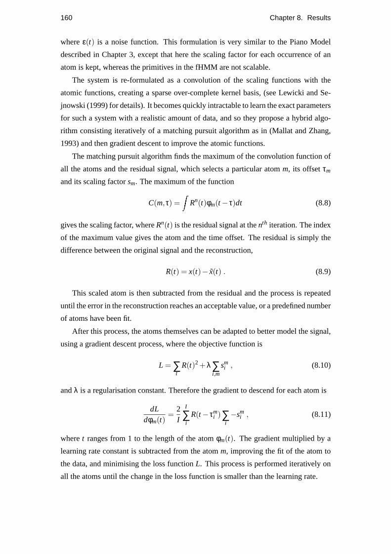
160 Chapter 8. Results
whereε(t) is a noise function. This formulation is very similar to the Piano Model
described in Chapter 3, except that here the scaling factor for each occurrence of an
atom is kept, whereas the primitives in the fHMM are not scalable.
The system is re-formulated as a convolution of the scaling functions with the
atomic functions, creating a sparse over-complete kernel basis, (see Lewicki and Se-
jnowski (1999) for details). It becomes quickly intractable to learn the exact parameters
for such a system with a realistic amount of data, and so they propose a hybrid algo-
rithm consisting iteratively of a matching pursuit algorithm as in (Mallat and Zhang,
1993) and then gradient descent to improve the atomic functions.
The matching pursuit algorithm finds the maximum of the convolution function of
all the atoms and the residual signal, which selects a particular atomm, its offsetτm
and its scaling factorsm. The maximum of the function
C(m,τ) =Z
Rn(t)φm(t− τ)dt (8.8)
gives the scaling factor, whereRn(t) is the residual signal at thenth iteration. The index
of the maximum value gives the atom and the time offset. The residual is simply the
difference between the original signal and the reconstruction,
R(t) = x(t)− x(t) . (8.9)
This scaled atom is then subtracted from the residual and the process is repeated
until the error in the reconstruction reaches an acceptable value, or a predefined number
of atoms have been fit.
After this process, the atoms themselves can be adapted to better model the signal,
using a gradient descent process, where the objective function is
L = ∑t
R(t)2 +λ∑i,m
smi , (8.10)
andλ is a regularisation constant. Therefore the gradient to descend for each atom is
dLdφm(t)
=2I
I
∑i
R(t− τmi )∑
i−sm
i , (8.11)
wheret ranges from 1 to the length of the atomφm(t). The gradient multiplied by a
learning rate constant is subtracted from the atomm, improving the fit of the atom to
the data, and minimising the loss functionL. This process is performed iteratively on
all the atoms until the change in the loss function is smaller than the learning rate.
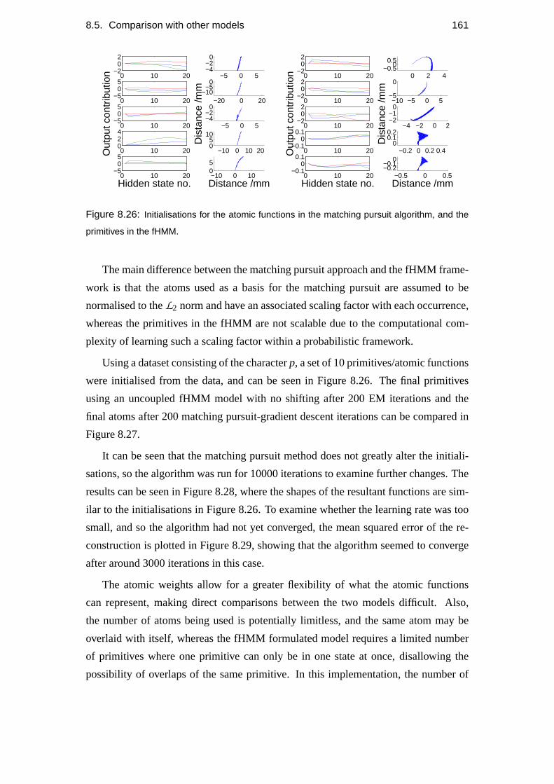
8.5. Comparison with other models 161
0 10 20−2
02
−5 0 5−4−2
0
0 10 20−5
05
−20 0 20−10
−50
0 10 20−5
05
Out
put c
ontr
ibut
ion
−5 0 5−4−2
0
Dis
tanc
e /m
m
0 10 20024
−10 0 10 2005
10
0 10 20−5
05
Hidden state no.−10 0 1005
Distance /mm
0 10 20−2
02
0 2 4−0.5
00.5
0 10 20−2
02
−10 −5 0 5−5
0
0 10 20−2
02
Out
put c
ontr
ibut
ion
−4 −2 0 2−2−1
0
Dis
tanc
e /m
m
0 10 20−0.1
00.1
−0.2 0 0.2 0.40
0.10.2
0 10 20−0.1
00.1
Hidden state no.−0.5 0 0.5
−0.2−0.1
0
Distance /mm
Figure 8.26: Initialisations for the atomic functions in the matching pursuit algorithm, and the
primitives in the fHMM.
The main difference between the matching pursuit approach and the fHMM frame-
work is that the atoms used as a basis for the matching pursuit are assumed to be
normalised to theL2 norm and have an associated scaling factor with each occurrence,
whereas the primitives in the fHMM are not scalable due to the computational com-
plexity of learning such a scaling factor within a probabilistic framework.
Using a dataset consisting of the characterp, a set of 10 primitives/atomic functions
were initialised from the data, and can be seen in Figure 8.26. The final primitives
using an uncoupled fHMM model with no shifting after 200 EM iterations and the
final atoms after 200 matching pursuit-gradient descent iterations can be compared in
Figure 8.27.
It can be seen that the matching pursuit method does not greatly alter the initiali-
sations, so the algorithm was run for 10000 iterations to examine further changes. The
results can be seen in Figure 8.28, where the shapes of the resultant functions are sim-
ilar to the initialisations in Figure 8.26. To examine whether the learning rate was too
small, and so the algorithm had not yet converged, the mean squared error of the re-
construction is plotted in Figure 8.29, showing that the algorithm seemed to converge
after around 3000 iterations in this case.
The atomic weights allow for a greater flexibility of what the atomic functions
can represent, making direct comparisons between the two models difficult. Also,
the number of atoms being used is potentially limitless, and the same atom may be
overlaid with itself, whereas the fHMM formulated model requires a limited number
of primitives where one primitive can only be in one state at once, disallowing the
possibility of overlaps of the same primitive. In this implementation, the number of
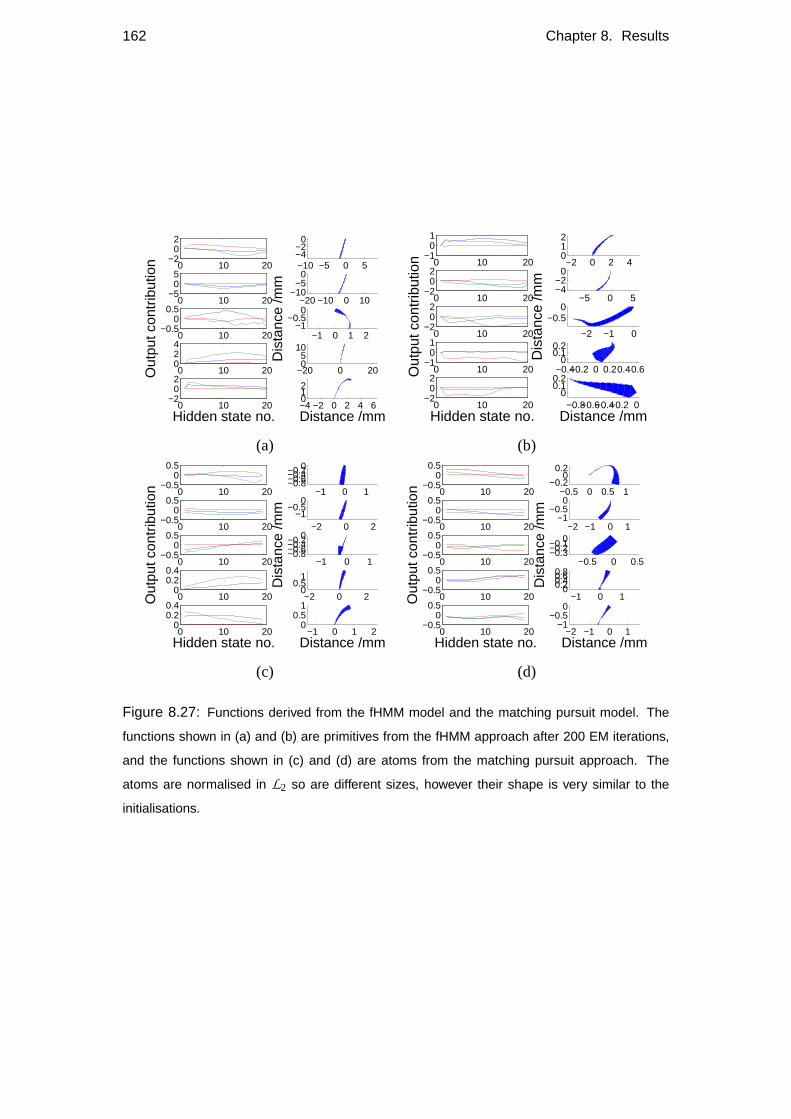
162 Chapter 8. Results
0 10 20−2
02
−10 −5 0 5−4−2
0
0 10 20−5
05
−20 −10 0 10−10
−50
0 10 20−0.5
00.5
Out
put c
ontr
ibut
ion
−1 0 1 2−1
−0.50
Dis
tanc
e /m
m
0 10 20024
−20 0 2005
10
0 10 20−2
02
Hidden state no.−4 −2 0 2 4 6012
Distance /mm
0 10 20−1
01
−2 0 2 4012
0 10 20−2
02
−5 0 5−4−2
0
0 10 20−2
02
Out
put c
ontr
ibut
ion
−2 −1 0
−0.50
Dis
tanc
e /m
m
0 10 20−1
01
−0.4−0.2 0 0.20.40.60
0.10.2
0 10 20−2
02
Hidden state no.−0.8−0.6−0.4−0.2 0
00.10.2
Distance /mm
(a) (b)
0 10 20−0.5
00.5
−1 0 1−0.8−0.6−0.4−0.20
0 10 20−0.5
00.5
−2 0 2−1
−0.50
0 10 20−0.5
00.5
Out
put c
ontr
ibut
ion
−1 0 1−0.8−0.6−0.4−0.20
Dis
tanc
e /m
m
0 10 200
0.20.4
−2 0 20
0.51
0 10 200
0.20.4
Hidden state no.−1 0 1 2
00.5
1
Distance /mm
0 10 20−0.5
00.5
−0.5 0 0.5 1−0.2
00.2
0 10 20−0.5
00.5
−2 −1 0 1−1
−0.50
0 10 20−0.5
00.5
Out
put c
ontr
ibut
ion
−0.5 0 0.5−0.3−0.2−0.10
Dis
tanc
e /m
m
0 10 20−0.5
00.5
−1 0 100.20.40.60.8
0 10 20−0.5
00.5
Hidden state no.−2 −1 0 1
−1−0.5
0
Distance /mm
(c) (d)
Figure 8.27: Functions derived from the fHMM model and the matching pursuit model. The
functions shown in (a) and (b) are primitives from the fHMM approach after 200 EM iterations,
and the functions shown in (c) and (d) are atoms from the matching pursuit approach. The
atoms are normalised in L2 so are different sizes, however their shape is very similar to the
initialisations.
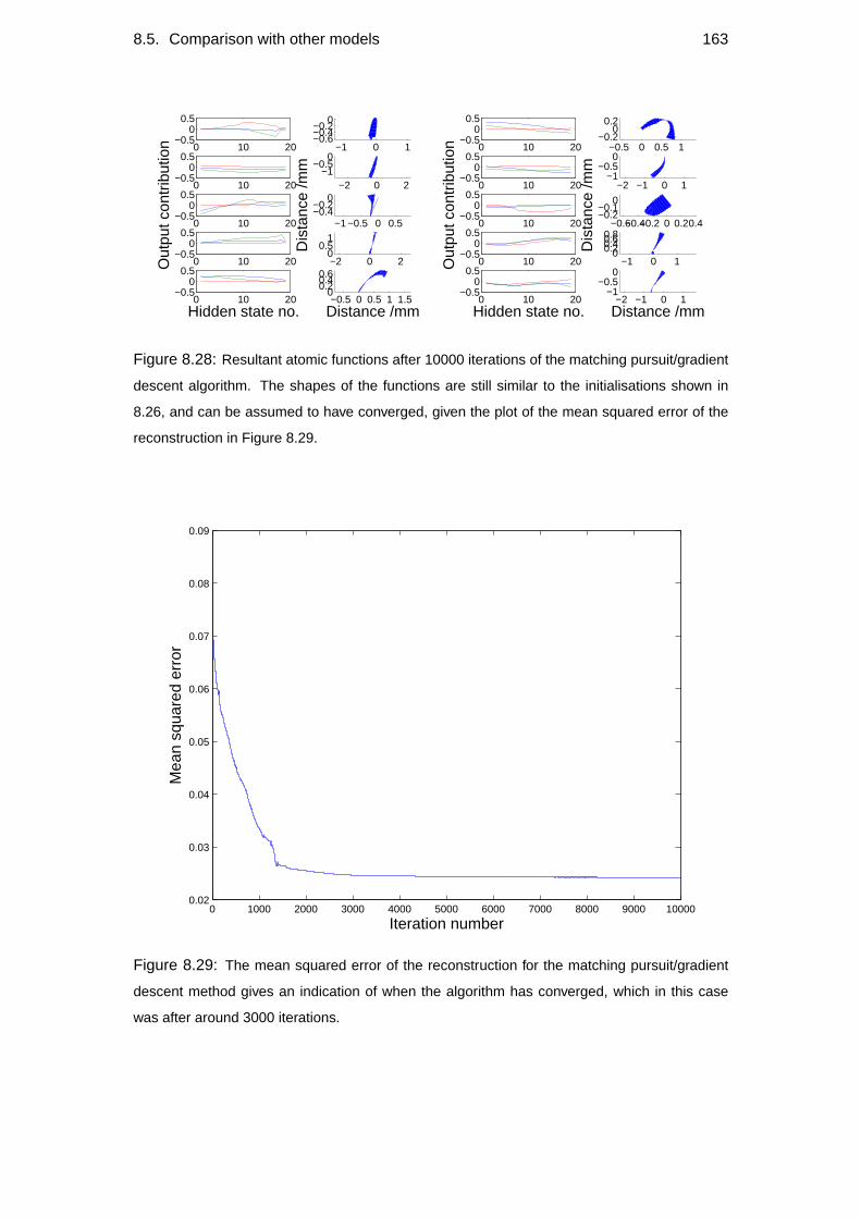
8.5. Comparison with other models 163
0 10 20−0.5
00.5
−1 0 1−0.6−0.4−0.2
0
0 10 20−0.5
00.5
−2 0 2−1
−0.50
0 10 20−0.5
00.5
Out
put c
ontr
ibut
ion
−1 −0.5 0 0.5−0.4−0.2
0
Dis
tanc
e /m
m
0 10 20−0.5
00.5
−2 0 20
0.51
0 10 20−0.5
00.5
Hidden state no.−0.5 0 0.5 1 1.5
00.20.40.6
Distance /mm
0 10 20−0.5
00.5
−0.5 0 0.5 1−0.2
00.2
0 10 20−0.5
00.5
−2 −1 0 1−1
−0.50
0 10 20−0.5
00.5
Out
put c
ontr
ibut
ion
−0.6−0.4−0.2 0 0.20.4−0.2−0.1
0
Dis
tanc
e /m
m
0 10 20−0.5
00.5
−1 0 100.20.40.60.8
0 10 20−0.5
00.5
Hidden state no.−2 −1 0 1
−1−0.5
0
Distance /mm
Figure 8.28: Resultant atomic functions after 10000 iterations of the matching pursuit/gradient
descent algorithm. The shapes of the functions are still similar to the initialisations shown in
8.26, and can be assumed to have converged, given the plot of the mean squared error of the
reconstruction in Figure 8.29.
0 1000 2000 3000 4000 5000 6000 7000 8000 9000 100000.02
0.03
0.04
0.05
0.06
0.07
0.08
0.09
Iteration number
Mea
n sq
uare
d er
ror
Figure 8.29: The mean squared error of the reconstruction for the matching pursuit/gradient
descent method gives an indication of when the algorithm has converged, which in this case
was after around 3000 iterations.
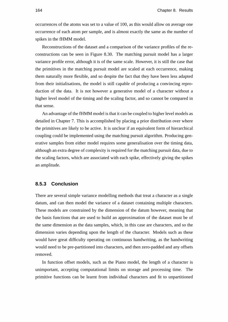
164 Chapter 8. Results
occurrences of the atoms was set to a value of 100, as this would allow on average one
occurrence of each atom per sample, and is almost exactly the same as the number of
spikes in the fHMM model.
Reconstructions of the dataset and a comparison of the variance profiles of the re-
constructions can be seen in Figure 8.30. The matching pursuit model has a larger
variance profile error, although it is of the same scale. However, it is still the case that
the primitives in the matching pursuit model are scaled at each occurrence, making
them naturally more flexible, and so despite the fact that they have been less adapted
from their initialisations, the model is still capable of producing a convincing repro-
duction of the data. It is not however a generative model of a character without a
higher level model of the timing and the scaling factor, and so cannot be compared in
that sense.
An advantage of the fHMM model is that it can be coupled to higher level models as
detailed in Chapter 7. This is accomplished by placing a prior distribution over where
the primitives are likely to be active. It is unclear if an equivalent form of hierarchical
coupling could be implemented using the matching pursuit algorithm. Producing gen-
erative samples from either model requires some generalisation over the timing data,
although an extra degree of complexity is required for the matching pursuit data, due to
the scaling factors, which are associated with each spike, effectively giving the spikes
an amplitude.
8.5.3 Conclusion
There are several simple variance modelling methods that treat a character as a single
datum, and can then model the variance of a dataset containing multiple characters.
These models are constrained by the dimension of the datum however, meaning that
the basis functions that are used to build an approximation of the dataset must be of
the same dimension as the data samples, which, in this case are characters, and so the
dimension varies depending upon the length of the character. Models such as these
would have great difficulty operating on continuous handwriting, as the handwriting
would need to be pre-partitioned into characters, and then zero-padded and any offsets
removed.
In function offset models, such as the Piano model, the length of a character is
unimportant, accepting computational limits on storage and processing time. The
primitive functions can be learnt from individual characters and fit to unpartitioned
8.5. Comparison with other models 165
−4−2024
−15
−10
−5
0
Dis
tanc
e /m
m
−4−202−15
−10
−5
0
−4−2024
−15−10
−50
−4−2024
−15
−10
−5
0
−4−202−15
−10
−5
0
−4−202−15
−10
−5
0
−4−202−15
−10
−5
0
−4−2024
−15−10
−50
Distance /mm−4−202
−15
−10
−5
0
−4−2024
−15
−10
−5
0
0 0.2 0.4 0.6 0.8 10
0.1
0.2
Time /s
x ve
loci
tyva
rianc
e
0 0.2 0.4 0.6 0.8 10
0.2
0.4
Time /s
y ve
loci
tyva
rianc
e
0 0.2 0.4 0.6 0.8 10
0.5
1
Time /sP
ress
ure
chan
ge
varia
nce
−4−202−15
−10
−5
0
Dis
tanc
e /m
m
−4−2024
−15−10
−50
−4−202−15−10
−50
−4−202−15
−10
−5
0
−6−4−2024
−20
−10
0
−6−4−2024−20
−10
0
−6−4−202−20
−10
0
−6−4−202
−15−10
−50
Distance /mm−4−202
−15
−10
−5
0
−4−2024−15−10
−50
0 0.2 0.4 0.6 0.8 10
0.2
0.4
Time /s
x ve
loci
tyva
rianc
e
0 0.2 0.4 0.6 0.8 10
0.5
Time /s
y ve
loci
tyva
rianc
e
0 0.2 0.4 0.6 0.8 10
0.5
1
Time /s
Pre
ssur
ech
ange
va
rianc
e
Figure 8.30: Reconstructions of a dataset containing the character p comparing two different
models. The top row shows reconstructions and the variance profile for reconstructions using
the fHMM model (with 5 primitives). The bottom row shows reconstructions and their variance
profile using the matching pursuit/gradient descent model, after 10000 iterations. The total
variance profile absolute error for the fHMM model was 12.02, whereas for the matching pursuit
model it was 14.36. These are not generative samples, and the variance profiles are taken from
the reconstructed dataset rather than a set of generated samples.
166 Chapter 8. Results
continuous segments of handwriting data, orvice versa. It could be argued that the
timing model needs to have partitioned characters to work, and for training purposes
this is indeed the case, as the timing model needs to be able to generalise across differ-
ent samples of the same character rather than generic handwriting samples. Because
the timing model is based upon a very sparse encoding of the characters, it is a much
simpler task to infer where the start of a character would be in spike timing space. A
very simple model based upon the specific combination of spikes within a short time
window at the start of a character would provide a very quick potential segmentation
function.
A further problem with the PCA/ICA models is that it is difficult for them to model
timing drift, as it corresponds to a shift in the dimensional representation of the data
when using a whole character as a datum. This type of timing jitter error is well
modelled in offset function models, and in Markov models, where it is possible for a
‘delay’ to be modelled by self transitions, which is known as dynamic time warping.
The matching pursuit model of Lewickiet al is very good when there are a large
number of potential atoms, such as a whole family of gamma-tone kernel functions.
Using a greedy cut-off process, a subset of these functions can then be selected and
adapted to better fit the dataset. The code produced is known as a spikegram, and
contains not just spike positions, but also spike amplitudes. This code is more com-
plex than the spike timing code of the fHMM, and can potentially have many more
atoms/primitives. This makes it difficult for a higher level model to generalise across
different character sample codes. For the case of an fHMM, it is possible to couple
the timing model and the primitive model together, providing a more generalised rep-
resentation. It is not clear how this would be implemented for the matching pursuit
case, as there is no probabilistic inference involved in the algorithm. However, the
matching pursuit algorithm is faster than EM inference performed on an fHMM. One
possible use of this could be to use the matching pursuit/gradient descent algorithm to
initialise the primitive shapes for the fHMM. The results of the matching pursuit al-
gorithm shown in Figure 8.28 suggest that the resultant atoms depend heavily on their
initialisations, or in the case of a whole set of functions, they would depend upon the
function class chosen.
Chapter 9
Discussion
This project has explored the possibility of modelling handwriting using a fixed func-
tion offset model (Piano Model). The aim of the project was to learn a generative
model for handwriting, based upon the concept of motor primitives. In the space of
pen movements, primitives were approximated as fixed functions in pen tip velocity
space.
Appropriate functions for such a model can be learnt within a formalised proba-
bilistic framework, using a constrained Factorial Hidden Markov Model. This frame-
work allows the functions to be variable lengths, and does not require traditional pre-
partitioning of the characters into points of highest curvature or any feature extraction,
which is often used in other handwriting models.
A generative model of characters based upon the primitive’s timing within a char-
acter was also presented. Several alternative models were investigated, although the
inconsistent nature of the spike timing data restricts the class of Gaussian models to be
one-dimensional.
Coupling of the primitive model together with the timing model during character
learning allows better representations of the data to be learnt, as the timing model
provides an informed onset prior distribution for the primitive model.
9.1 Implications for biology
The existence of motor primitives as sub-blocks of movement is a widely accepted
theory, partially because the definition of what exactly a primitive might be is flexible.
From a biological point of view, it is an attractive idea that primitives could resemble
an output basis set for controlling muscles, where the selection and timing of the prim-
167
168 Chapter 9. Discussion
itives is the encoded movement. This code would therefore naturally be representable
by a distributed set of spike timings, such as is likely to be the case in the brain.
One implication for biology, which is in agreement with several movement stud-
ies, focussing on rhythm representation an movement, is that the control of biological
movement may be segmented into a primitive part and a timing part. (Penhume et al.,
1998; Meegan et al., 2000; Dennis et al., 2004) all explore the importance of rhythm
in movement planning and generation, and the role of the cerebellum in motor timing
tasks.
Understanding how people might be learning to control a pen, and the internal
representations used could have useful educational implications. More efficient teach-
ing methods, perhaps focussing on rhythmic aspects of writing, with the purpose of
reinforcing the best possible timing code could be developed.
A related field to the teaching of handwriting is relearning to write, after a stroke,
or physical damage to the hand or arm. With a better understanding of how the brain
might have originally encoded the movements, the relearning process could be opti-
mised, making it easier and faster for the subject.
9.2 Implications for robotics
Instead of defining the observable data as pen tip velocities, it could be defined as
some parameterisation of a control system. These parameterisations could change in
a fixed manner over the course of the primitive, allowing complex movements to be
built up by combining primitives. Such primitives could be learnable using EM as
described in Chapter 4, along with a deterministic model of the control system. Sim-
ple one-dimensional timing variation could then represent the complex variation in
the movement trajectory of the system being controlled. A more specific formulation
would be to model the joint torques of some robot model as the observable variables,
and learn primitives based upon this data.
Robotic control is traditionally a feedback control loop problem, where some error
signal is fed back and along with a control or modulating signal is used to minimise the
predicted error. As the system being controlled becomes more complex, and as uncer-
tainty is introduced, this type of control becomes very difficult to plan and optimise.
More recent research into using motor primitives as a basis for control has generally fo-
cussed upon segmenting movements, and using some component extraction technique
to provide a basis set of movements. These techniques normally do not assume that
9.3. Implications for data representation 169
the components are time extended, or that they can overlap in an unrestricted fashion
(either entirely or partially) with each other. An extension of the model presented here
could be used as a framework to model and learn a novel type of motor primitive that
could be used to control a physical control system. The combinatorial variety of the
output possibilities is higher than in other models, as the same combination of primi-
tives can be triggered with different offsets, however the internal representation is very
compact, being a set of spike times.
It remains to be seen if such a primitive-timing representation could be useful for
adaptive control problems, however there are suggestions that biological, or at least
human control may rely on timing specific events. For instance research by David Lee
into tau theory of movement has shown how biological movements appear to be guided
by coupling time intervals observed in the dynamic world. (see (Lee et al., 2001), or
(Lee, 2006) for a review of this research). Tau theory suggests that the brain encodes
the dynamic world in terms of timings of events, and uses ratios of these timings to
adapt movements. The primitive-timing representation of movements would fit in well
with such a theory of movement control and planning.
9.3 Implications for data representation
Compression of data is an extremely important subject in the modern world, where
information and media are continually being stored, categorised, and transmitted over
the internet. Compression of data is also important for the brain, and so if the hand-
writing movements are produced using a similar model to the one described in this
project, it is likely that they are stored in the highly compressed form of spike times.
Such a code would therefore capture the recognisable variation in the handwriting, and
thus be the most efficient way of storing and transmitting the handwriting.
Many devices which use handwriting recognition, such as personal hand-held de-
vices, have a relatively low bandwidth connection, meaning the information transmit-
ted is normally in the form of text, rather than handwriting. However it may some-
times be more convenient or desirable to transmit the handwriting, or some illustrative
sketches. A primitive-timing representation of these pen movements would provide
a good compression for low bandwidth transmission. An interesting aspect of this
representation is the possibility of the sketch and writing being transformed into the
receiver’s handwriting upon receipt.
Handwriting is gradually becoming more of an art form, as people use keyboards
170 Chapter 9. Discussion
more and more, although this trend may not continue now that pen tablets in the form
of a small hand-held PC or personal organiser are becoming popular. Handwriting is
considered a very personal skill, with many ‘personality guessing tests’ based upon
handwriting. This means that it would be a good mode of interaction with many
computing devices. If the text on a mobile phone was a replication of the owner’s
handwriting for instance, a greater bond, or personalisation could be achieved.
9.4 Limitations/Extensions of the model
A limitation of the model is the lack of feedback, both in terms of the behaviour of the
primitives themselves, and any positional feedback to higher levels of the model. This
could potentially improve the performance, and make the primitives more generalised
as simple parameterised systems. A simplified model of a hand as a spring system
was proposed by (Hinton and Nair, 2005). Such a system would provide low level
feedback, and the primitive model would parameterise the stiffness of the springs over
time.
The primitives in a piano model formulation generally have a scaling factor asso-
ciated with them, however in the fHMM framework, they do not. This is because the
extra parameters would make the model extremely difficult to learn, and the structured
variational approximation used in this project to improve the speed of the EM infer-
ence would no longer work. An alternative form of posterior estimation such as Gibbs
sampling could be used on a more complex model, however the larger parameter space
would bring with it more local maxima in the likelihood function, making inference
difficult.
A problem for any possible timing model is that the primitives are allowed to occur
a variable number of times in a particular character sample. This means that the tim-
ing model needs a latent state modelling primitive presence, and makes it difficult to
capture the covariance between the spike times. Forcing all primitives to occur exactly
once in a character sample would be possible by imposing very strong priors at the start
and the end of a character. This would create a sort of ‘Serialist Piano Model’1 where
primitives are not as flexible as in the model proposed here. Each character would
have to contain every primitive. This could work for a single character class, but for
multiple character types different primitives would have to be switched on or off, po-
1Serialism is a 20th century compositional technique whereby every semitone in a scale must beplayed exactly once before repetitions are allowed.
9.4. Limitations/Extensions of the model 171
tentially achieved by using a single probabilistic binary onset parameter dependent
upon the character class. With this constrained primitive model a timing model would
be a simple case of placing a single multivariate Gaussian distribution or a mixture of
Gaussians over all the spike times for a particular character. Preliminary experiments
however showed that such a model still produced multiple clusters of spikes, with some
character samples using a primitive from cluster 1, and some using the same primitive
from cluster 2 for instance. The extra constraints placed on the model simply mean
that more primitives are required to produce an acceptable reconstruction. Such a dis-
tribution could be modelled using a mixture of Gaussians, and a higher level model
coupling the components of the various primitives together, however this is really the
same situation as with the current model, but with more primitives occurring fewer
times.
The low level primitive model works well to produce a reconstruction of the dataset,
assuming an adequate number of primitives. However the generative performance of
the timing models are not very good when large numbers of primitives are needed.
By fixing the hidden state trajectory of the timing model, as was discussed in Section
6.2.4.2, it can be seen that there should be more dependencies between the primitives.
As the primitives are encoded as spikes, a probabilistic spiking neural network would
be an interesting model to try. Connectivity in the network would determine depen-
dency between primitives, and multiple synaptic time delays could model the timing
of the spikes. Alternatively, the current mode data could be used to extend the model
to another level, by modelling this data.
A very successful and widely used method of component extract is ICA. The prob-
lem with applying this approach to primitives is that the primitives must be ‘keyed’,
in that their starting point must be known in each sample. The fHMM model acts in a
similar manner to ICA, trying to extract the most statistically independent components
or factors. The benefit of the constrained fHMM presented in this project is that the fac-
tors have no pre-defined start points. The similarities with ICA would be interesting to
explore further. Using longer primitives that must occur once in a sample, and that have
an associated scaling factor would perhaps provide similar independent components to
ICA. However the components derived by the fHMM would be less constrained, and
self-transitions could easily be introduced. A quick exploration of this approach was
implemented by using fixed length primitives of 150 states, (the equivalent of 0.75s)
which is of the same order of length as the character samples. 5 long primitives were
initialised randomly and trained upon a dataset containing the characterp, and can be
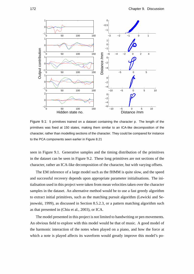
172 Chapter 9. Discussion
0 50 100 150−1
0
1
−3 −2 −1 0 1
−1
−0.5
0
0 50 100 150−1
0
1
−6 −4 −2 0 2 4
−1
0
1
0 50 100 150−1
0
1
Out
put c
ontr
ibut
ion
−5 0 5
−4
−2
0
Dis
tanc
e /m
m
0 50 100 150−1
0
1
−10 −5 0 5 10
−4
−2
0
0 50 100 150−2
0
2
Hidden state no.−10 −5 0 5 10
−6
−4
−2
0
Distance /mm
Figure 9.1: 5 primitives trained on a dataset containing the character p. The length of the
primitives was fixed at 150 states, making them similar to an ICA-like decomposition of the
character, rather than modelling sections of the character. They could be compared for instance
to the PCA components seen earlier in Figure 8.21
seen in Figure 9.1. Generative samples and the timing distribution of the primitives
in the dataset can be seen in Figure 9.2. These long primitives are not sections of the
character, rather an ICA-like decomposition of the character, but with varying offsets.
The EM inference of a large model such as the fHMM is quite slow, and the speed
and successful recovery depends upon appropriate parameter initialisations. The ini-
tialisation used in this project were taken from mean velocities taken over the character
samples in the dataset. An alternative method would be to use a fast greedy algorithm
to extract initial primitives, such as the matching pursuit algorithm (Lewicki and Se-
jnowski, 1999), as discussed in Section 8.5.2.3, or a pattern matching algorithm such
as that presented in (Chiu et al., 2003), or ICA.
The model presented in this project is not limited to handwriting or pen movements.
An obvious field to explore with this model would be that of music. A good model of
the harmonic interaction of the notes when played on a piano, and how the force at
which a note is played affects its waveform would greatly improve this model’s po-

9.4. Limitations/Extensions of the model 173
0 0.2 0.4 0.6 0.8 1 1.2
1
2
3
4
5
Time /s
Prim
itive
num
ber
p
−4−202−15
−10
−5
0
Dis
tanc
e /m
m
−4−202−15
−10
−5
0
−4−2024−15−10
−50
−4−202−15−10
−50
−4−202
−10
−5
0
−202
−10
−5
0
−4−202−15−10
−50
−4−202
−10
−5
0
Distance /mm−4−202
−15
−10
−5
0
−4−202−15
−10
−5
0
Figure 9.2: The timing of the long primitives seen in Figure 9.1 can be seen in the leftmost
plot, showing that they are mostly all active for every character sample, and at most a single
time. The rightmost plot shows 10 generative samples, which are expectably good, due to the
simplicity of the timing distribution.
tential to represent and reproduce piano music, and potentially provide a very efficient
and convincingperformance enginefor reproduction of simple MIDI scores.
9.4.1 Psychophysical experiments
Validation of the primitives and their presence in the brain could be attempted by per-
forming some perceptual experiments. Each task would require the subject to provide
handwriting samples upon which the model would be trained, and then subject specific
tasks using ‘their’ primitives could be performed. Several psychophysical experiments
would be interesting to perform in conjunction with the handwriting model presented
here. Such experiments would explore the permanence of the primitive functions, and
whether they are also exploited for recognition purposes.
Learning to write
The subject would be asked to learn to reproduce a novel character. Either the character
could be built up using primitives extracted from their writing, or entirely different
primitives. The assumption being that the task in the later case would be more difficult
for the subject. A further experiment would be to then train a new model on the novel
character samples, and compare the primitives extracted with the ones used to generate
the character originally. The assumption being that the differences between theplanted
motifsand the extracted primitives would shed light on the limitations of the types of
primitive functions that are learnable.
174 Chapter 9. Discussion
Finally, depending upon the rate at which a subject learns to write a new character,
an analysis of the primitives present over time would be very interesting, as it is unclear
when, how and if primitives might be adapted to a specific task.
Learning to read
A subject would be required to learn two or more novel characters, and then distinguish
between them. One set of characters would be constructed using primitives extracted
from their handwriting, whilst another set would be constructed using novel primitives.
The assumption being that if primitives are exploited in some way for recognition, then
the set with their own primitives would be easier to learn.
Learning to remember
A subject would be presented with a single, novel character, and then asked to recall
it by using a differentiation task after a wait period. Similar to the above experiments,
the character would either be made up using the subject’s primitives, or novel ones.
A variation on this experiment could be to introduce noise into the character be-
tween the presentations, either as primitive shape noise, or primitive timing noise. The
hypothesis here is that the timing noise would be more noticeable, as small variations
in the primitive shapes might not be ‘seen’ by a feature detector trained upon a partic-
ular primitive.
9.5 Summary
Despite having superior motors and materials, with far less noise present in actuators
and sensors, robots are still much worse at moving than biological organisms. This
must be therefore due to a superior internal representation of the movements being
made. This thesis has attempted to shed light on one such possible representation
based upon the concept of primitives.
Primitives allow small sections of movement to be assembled to create complete
task based movements. The manner in which these primitives are assembled, and the
adaptability of the primitives is unknown. This thesis assumes that the brain operates in
a massively parallel and asynchronous manner, meaning that the primitives are likely
to be triggered at different times throughout a movement, and that the timing of these
events would contain noise.
9.5. Summary 175
This thesis attempts to explain handwriting variation in terms of noise within the
generating model, or timing jitter of primitive activation. Other sources of varia-
tion such as primitive substitution are partially modelled, and an interesting extension
would be to examine how much unexplained variation could be accounted for by dy-
namical models of the hand.
Despite learning to handwrite in classes with a common teacher, and identical
teaching materials and methods, personal handwriting develops much variation, both
from a single subject, and style variation between subjects. This thesis attempts to ex-
plain the first type of variation in terms of primitive timing noise, and the larger second
type of variation in terms of differences in primitive shapes between subjects.
The timing of primitives can conveniently be expressed as a spike timing pattern,
which is a very compact code for a character. It holds obvious similarities to the spiking
behaviour of neuronal activity, and suggests a segmentation between a timing model
and a primitive model within the brain. Interesting lesion studies could be conducted
by carrying out simulated lesions of the model to validate the type of primitives used
here. Also this model allows several psycho-physical experiments to be conducted to
further examine the nature of primitives and the operation of motor planning within
the brain.
In conclusion, this thesis provides a novel manner of inferring primitives from time
series movement data, in this case handwriting trajectories. This model also attempts
to generalise across multiple samples to produce a fully generative model of the move-
ment, where the complex variation from one sample to the next is captured in the
higher level timing model as simple Gaussian noise. It is the hope of this author that
such a model will prove useful for new types of robotic movement planning, and for
efficient handwriting representation and reproduction.

Chapter 10
Appendix
10.1 Variational Log Likelihood
The observable data likelihood is defined as,
logP({Yt}) = log ∑{Sm
t }P({Sm
t ,Yt})
= log ∑{Sm
t }Q({Sm
t })[
P({Smt ,Yt})
Q({Smt })
]≥ ∑{Sm
t }Q({Sm
t }) log
[P({Sm
t ,Yt})Q({Sm
t })
](10.1)
The inequality defines a lower bound on the likelihood, called the variational log like-
lihood (VLL), which is equivalent to the negative variational free energy.
VLL = ∑{Sm
t }Q({Sm
t }) logP({Smt ,Yt})− ∑
{Smt }
Q({Smt }) logQ({Sm
t }) . (10.2)
The various terms of this equation are derived here. The joint probability of the hidden
and observable states of the fHMM can be expanded,
logP({Smt ,Yt}) = ∑
mlogP(Sm
1 )+∑m
T
∑t=2
logP(Smt |Sm
t−1)+T
∑t=1
logP(Yt |S1t , ..,S
Mt )
= ∑m
logπππmSm
1+∑
m
T
∑t=2
logPmSm
t ,Smt−1
+T
∑t=1
logP(Yt |S1t , ..,S
Mt ),
(10.3)
177
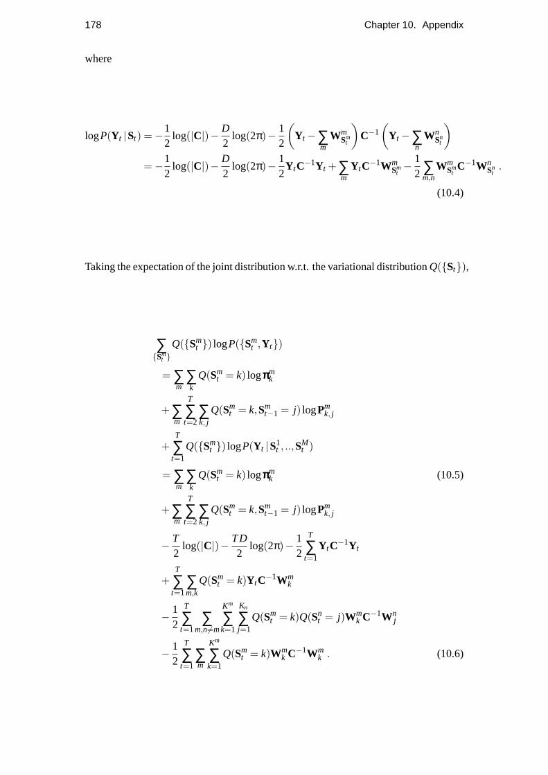
178 Chapter 10. Appendix
where
logP(Yt |St) =−12
log(|C|)− D2
log(2π)− 12
(Yt−∑
mWm
Smt
)C−1
(Yt−∑
nWn
Snt
)=−1
2log(|C|)− D
2log(2π)− 1
2YtC−1Yt +∑
mYtC−1Wm
Smt− 1
2 ∑m,n
WmSm
tC−1Wn
Snt.
(10.4)
Taking the expectation of the joint distribution w.r.t. the variational distributionQ({St}),
∑{Sm
t }Q({Sm
t }) logP({Smt ,Yt})
= ∑m
∑k
Q(Smt = k) logπππm
k
+∑m
T
∑t=2
∑k, j
Q(Smt = k,Sm
t−1 = j) logPmk, j
+T
∑t=1
Q({Smt }) logP(Yt |S1
t , ..,SMt )
= ∑m
∑k
Q(Smt = k) logπππm
k (10.5)
+∑m
T
∑t=2
∑k, j
Q(Smt = k,Sm
t−1 = j) logPmk, j
− T2
log(|C|)− TD2
log(2π)− 12
T
∑t=1
YtC−1Yt
+T
∑t=1
∑m,k
Q(Smt = k)YtC−1Wm
k
− 12
T
∑t=1
∑m,n6=m
Km
∑k=1
Kn
∑j=1
Q(Smt = k)Q(Sn
t = j)Wmk C−1Wn
j
− 12
T
∑t=1
∑m
Km
∑k=1
Q(Smt = k)Wm
k C−1Wmk . (10.6)
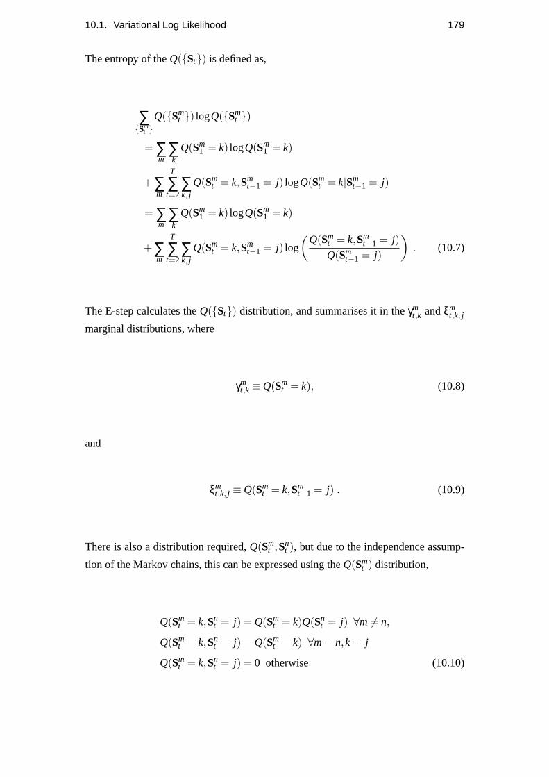
10.1. Variational Log Likelihood 179
The entropy of theQ({St}) is defined as,
∑{Sm
t }Q({Sm
t }) logQ({Smt })
= ∑m
∑k
Q(Sm1 = k) logQ(Sm
1 = k)
+∑m
T
∑t=2
∑k, j
Q(Smt = k,Sm
t−1 = j) logQ(Smt = k|Sm
t−1 = j)
= ∑m
∑k
Q(Sm1 = k) logQ(Sm
1 = k)
+∑m
T
∑t=2
∑k, j
Q(Smt = k,Sm
t−1 = j) log
(Q(Sm
t = k,Smt−1 = j)
Q(Smt−1 = j)
). (10.7)
The E-step calculates theQ({St}) distribution, and summarises it in theγmt,k andξm
t,k, j
marginal distributions, where
γmt,k ≡Q(Sm
t = k), (10.8)
and
ξmt,k, j ≡Q(Sm
t = k,Smt−1 = j) . (10.9)
There is also a distribution required,Q(Smt ,Sn
t ), but due to the independence assump-
tion of the Markov chains, this can be expressed using theQ(Smt ) distribution,
Q(Smt = k,Sn
t = j) = Q(Smt = k)Q(Sn
t = j) ∀m 6= n,
Q(Smt = k,Sn
t = j) = Q(Smt = k) ∀m= n,k = j
Q(Smt = k,Sn
t = j) = 0 otherwise (10.10)
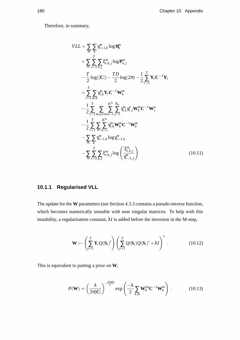
180 Chapter 10. Appendix
Therefore, in summary,
VLL = ∑m
∑k
γmt=1,k logπππm
k
+∑m
T
∑t=2
∑k, j
ξmt,k, j logPm
k, j
− T2
log(|C|)− TD2
log(2π)− 12
T
∑t=1
YtC−1Yt
+T
∑t=1
∑m,k
γmt,kYtC−1Wm
k
− 12
T
∑t=1
∑m,n6=m
Km
∑k=1
Kn
∑j=1
γmt,kγn
t, jWmk C−1Wn
j
− 12
T
∑t=1
∑m
Km
∑k=1
γmt,kW
mk C−1Wm
k
−∑m
∑k
γmt=1,k logγm
t=1,k
−∑m
T
∑t=2
∑k, j
ξmt,k, j log
(ξm
t,k, j
γmt−1, j
)(10.11)
10.1.1 Regularised VLL
The update for theW parameters (see Section 4.3.3 contains a pseudo-inverse function,
which becomes numerically unstable with near singular matrices. To help with this
instability, a regularisation constant,λI is added before the inversion in the M-step,
W←
(T
∑t=1
YtQ(St)′)(
T
∑t=1
Q(St)Q(St)′+λI
)†
. (10.12)
This is equivalent to putting a prior onW,
P(W) =(
λ2π|C|
)−KMD2
exp
(−λ2 ∑
k,m
W′mk C−1Wmk
). (10.13)
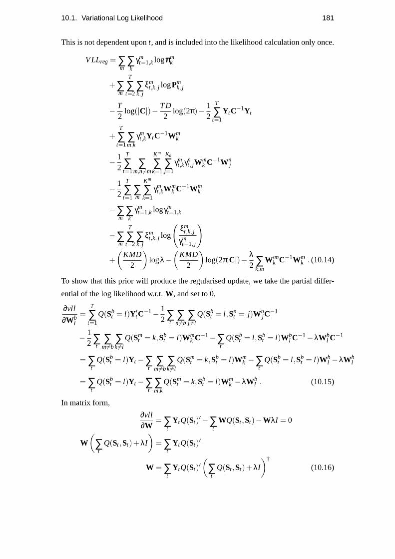
10.1. Variational Log Likelihood 181
This is not dependent upont, and is included into the likelihood calculation only once.
VLLreg = ∑m
∑k
γmt=1,k logπππm
k
+∑m
T
∑t=2
∑k, j
ξmt,k, j logPm
k, j
− T2
log(|C|)− TD2
log(2π)− 12
T
∑t=1
YtC−1Yt
+T
∑t=1
∑m,k
γmt,kYtC−1Wm
k
− 12
T
∑t=1
∑m,n6=m
Km
∑k=1
Kn
∑j=1
γmt,kγn
t, jWmk C−1Wn
j
− 12
T
∑t=1
∑m
Km
∑k=1
γmt,kW
mk C−1Wm
k
−∑m
∑k
γmt=1,k logγm
t=1,k
−∑m
T
∑t=2
∑k, j
ξmt,k, j log
(ξm
t,k, j
γmt−1, j
)
+(
KMD2
)logλ−
(KMD
2
)log(2π|C|)− λ
2 ∑k,m
W′mk C−1Wmk . (10.14)
To show that this prior will produce the regularised update, we take the partial differ-
ential of the log likelihood w.r.t.W, and set to 0,
∂vll
∂Wbl
=T
∑t=1
Q(Sbt = l)Y′tC
−1− 12∑
t∑n6=b
∑j 6=l
Q(Sbt = l ,Sn
t = j)Wnj C−1
− 12∑
t∑
m6=b∑k6=l
Q(Smt = k,Sb
t = l)Wmk C−1−∑
tQ(Sb
t = l ,Sbt = l)Wb
l C−1−λWbl C−1
= ∑t
Q(Sbt = l)Yt−∑
t∑
m6=b∑k6=l
Q(Smt = k,Sb
t = l)Wmk −∑
tQ(Sb
t = l ,Sbt = l)Wb
l −λWbl
= ∑t
Q(Sbt = l)Yt−∑
t∑m,k
Q(Smt = k,Sb
t = l)Wmk −λWb
l . (10.15)
In matrix form,
∂vll∂W
= ∑t
YtQ(St)′−∑t
WQ(St ,St)−WλI = 0
W(
∑t
Q(St ,St)+λI
)= ∑
tYtQ(St)′
W = ∑t
YtQ(St)′(
∑t
Q(St ,St)+λI
)†
(10.16)

Bibliography
R. Amit and M. Mataric. Parametric primitives for motor representation and control.
In Proceedings of the IEEE International Conference on Robotics and Automation,
pages 863–868, 2002.
L. E. Baum, T. Petrie, G. Soules, and N. Weiss. A maximization technique occurring
in the statistical analysis of probabilistic functions of markov chains.Ann. Math.
Statist., 40(1):164–171, 1970.
H. S. M. Beigi. An overview of handwriting recognition. In1st Annual conference
on technological advancements in developing countries, pages 30–46, Columbia
University, New York, July 1993.
E. Bizzi, S.F. Giszter, E. Loeb, F.A. Mussa-Ivaldi, and P. Saltiel. Modular organization
of motor behavior in the frog’s spinal cord.Trends in Neurosciences, 18(10):442–
446, 1995.
E. Bizzi, A. d’Avella, P. Saltiel, and M. Trensch. Modular organization of spinal motor
systems.The Neuroscientist, 8(5):437–442, 2002.
G. Caithness, R. Osu, P. Bays, H. Chase, J. Klassen, M. Kawato, D. M. Wolpert,
and J. R. Flanagan. Failure to consolidate the consolidation theory of learning for
sensorimotor adaptation tasks.Journal of Neuroscience, 24(40):8662–8671, 2004.
A. Cemgil, B. Kappen, and D. Barber. A generative model for music transcription. In
IEEE Transactions on Speech and Audio Processing, volume 13, 2005.
B. Chiu, E. Keogh, and S. Lonardi. Probabilistic discovery of time series motifs, 2003.
P.Perona D. del Vecchio, R.M. Murray. Decomposition of human motion into
dynamics-based primitives with application to drawing tasks.Automatica, 39:2085–
2098, 2003.
183

184 Bibliography
A. d’Avella and E. Bizzi. Shared and specific muscle synergies in natural motor be-
haviors. InNational Academy of Sciences, volume 102, pages 3076–3081, 2005.
A. d’Avella and E. Bizzi. Low dimensionality of supraspinally induced force fields.
Proc. Natl. Acad. Sci. USA, 96:7711–7714, 1998.
A. d’Avella, P. Saltiel, and E. Bizzi. Combinations of muscle synergies in the con-
struction of a natural motor behavior.Nature Neuroscience, 6(3):300–308, 2003.
P. R. Davidson and D. M. Wolpert. Motor learning and prediction in a variable envi-
ronment.Curr. Opinion in Neurobiology, 13:1–6, 2003.
P. R. Davidson and D. M. Wolpert. Scaling down motor memories: de-adaptation after
motor learning.Neuroscience Letters, 370:102–107, 2004.
A. Rizzi D.C. Conner, H. Choset. Integrated planning and control for convex-bodied
nonholonomic systems using local feedback. InRobotics: Science and Systems II,
MIT Press, pages 57–64, 2006.
M. Dennis, K. Edelstein, R. Hetherington, K. Copeland, J. Frederick, S. E. Blaser, L.A.
Kramer, J.M. Drake, M. Brandt, and J. M. Fletcher. Neurobiology of perceptual and
motor timing in children with spina bifida in relation to cerebellar volume.Brain,
2004.
E. Drumwright, O. C. Jenkins, and M. J. Mataric. Exemplar-based primitives for hu-
manoid movement classification and control. InIn Proc. of Intl. Conf. on Robotics
and Automation, pages 140–145, 2004.
A. Fod, M.J. Mataric, and O.C. Jenkins. Automated derivation of primitives for move-
ment classification.Autonomous robots, 12(1):39–54, 2002.
V. Gallese, L. Fadiga, L. Fogassi, and G. Rizzolatti. Action recognition in the premotor
cortex.Brain, 119:593–609, 1996.
Z. Ghahramani and M.I. Jordan. Factorial hidden Markov models.Machine Learning,
29:245–275, 1997.
A. Hamilton, K. Jones K, and D. M. Wolpert. The scaling of motor noise with muscle
size and motor unit number.Experimental Brain Research, 157:417–430, 2004.
Bibliography 185
G. E. Hinton and V. Nair. Inferring motor programs from images of handwritten digits.
In Advances in Neural Information Processing Systems, pages 515–522, 2005.
A. Hyvarinen. Survey on independent component analysis.Neural Computing Surveys,
2:94–128, 1999.
A. Ijspeert, J. Nakanishi, and S. Schaal. Learning attractor lanscapes for motor prim-
itives. In Advances in Neural Information Processing Systems, volume 15, pages
1523–1530, 2003.
W.J. Kargo and S.F. Giszter. Rapid corrections of aimed movements by combination
of force-field primitives.J. Neurosci., 20:409–426, 2000.
Y. Karklin and M. S. Lewicki. A hierarchical bayesian model for learning non-linear
statistical regularities in non-stationary natural signals.Neural Computation, 17(2):
397–423, 2005.
O. D. Kharraz-Tavakol, T. Eggert, N. Mai, and A. Straube. Learning to write letters:
transfer in automated movements indicates modularity of motor programs in human
subjects.Neurosci Lett., 17(1-2):33–36, 2000.
K. P. Kording, S. Ku, and D. M. Wolpert. Bayesian integration in force estimation.
Journal of Neurophysiology, 92:3161–3165, 2004.
D.M. Lee. How movement is guided. http://www.perception-in-
action.ed.ac.uk/PDFs/Howmovementisguided.pdf, 2006.
D.N. Lee, A.P. Georgopoulos, M.J. Clark, C.M. Craig, and N.L. Port. Guiding contact
by coupling the taus of gaps.Exp. Brain Res., 139(2):151–159, 2001.
M. S. Lewicki and T. J. Sejnowski. Coding time-varying signals using sparse shift-
invariant representations.Advances in Neural Information Processing Systems, 11:
730–736, 1999.
S. G. Mallat and Z. Zhang. Matching pursuits with time-frequency dictionaries.IEEE
Transactions on Signal Processing, 41(12):3397–3415, 1993.
C. Marquardt, W. Gentz, and N. Mai. Visual control of automated handwriting move-
ments.Exp. Brain Research, 128:224–228, 1999.
186 Bibliography
M.J. Mataric. Primitives-based humanoid control and imitation. Technical report,
DARPA MARS project, 2004.
D.V. Meegan, R.N. Aslin, and R. A. Jacobs. Motor timing learned without motor
training. Nature Neuroscience, 3(9):860–862, 2000.
R. G. J. Meulenbroek and A. W. A. Van Gemmert. Advances in the study of drawing
and handwriting.Human movement science, 22:131–220, 2003.
R.G.J. Meulenbroek, D.A. Rosenbaum, A.J.W.M. Thomassen, L.D. Loukopoulos, and
J. Vaughan. Adaptation of a reaching model to handwriting: How different effectors
can produce the same written output, and other results.Psychological Research, 59
(1):64–74, 1996.
F.A. Mussa-Ivaldi and E. Bizzi. Motor learning through the combination of primitives.
Phil. Trans. R. Soc. Lond., 355:1755–1769, 2000.
C. Padoa-Schioppa, C. S. R. Li, and E. Bizzi. Neuronal correlates of kinematics-to-
dynamics transformation in the supplementary motor area.Neuron, 36:751–765,
November 2002.
V.B. Penhume, R.J. Zatorre, and A.C. Evans. Cerebellar contributions to motor tim-
ing: A pet study of auditory and visual rythm reproduction.Journal of Cognative
Neuroscience, 10(6):752–765, 1998.
L. R. Rabiner. A tutorial on hidden markov models and selected applications in speech
recognition. InInstitute of Electrical and Electronic Engineers, volume 77, pages
257–286, 1989.
J.O. Ramsay. Functional components of variation in handwriting.Journal of the Amer-
ican Statistical Association, 95:9–15, 2000.
S. Roweis and A. Alwan. Towards articulatory speech recognition: Learning smooth
maps to recover articulator information. InProc. Eurospeech97, pages 1227–1230,
1997.
S. Schaal, J. Peters, J. Nakanishi, and A. Ijspeert. Learning movement primitives. In
International Symposium of Robotics Research, 2004.
Y. Singer and N. Tishby. Dynamical encoding of cursive handwriting.Journal Biolog-
ical Cybernetics, 71(3):227–237, July 1994.
Bibliography 187
E. Smith and M. S. Lewicki. Efficient coding of time-relative structure using spikes.
Neural Computation, 17(1):19–45, 2005.
S.M. LaVille S.R. Lindemann. Smoothly blending vector fields for global robot navi-
gation. InIEEE Conference Decision and Control, 2005.
A.A. Handzel T. Flash. Affine differential geometry analysis of human arm move-
ments.Biological Cybernetics, 96:577–601, 2007.
E. Todorov and M.I. Jordan. Optimal feedback control as a theory of motor coordina-
tion. Nature Neuroscience, 5(11):1226–1235, 2002.
R. J. van Beers, P Haggard, and D. M. Wolpert. The role of exucution noise in move-
ment variability.J. Neurophysiol., 91:1050–1063, 2004.
A. Vinciarelli and S. Bengio. Offline cursive word recognition using continuous den-
sity hidden Markov models trained with pca or ica features. In16 th International
Conference on Pattern Recognition, volume 3, 2002.
B.H. Williams, M.Toussaint, and A.J. Storkey. Extracting motion primitives from nat-
ural handwriting data. InInternational Conference on Artificial Neural Networks,
volume 2, pages 634–643, 2006.
B.H. Williams, M.Toussaint, and A.J. Storkey. A primitive based generative model to
infer timing information in unpartitioned handwriting data. InInternational Joint
Conference on Artificial Intelligence, pages 1119–1124, 2007.
B.H. Williams, M. Toussaint, and A.J. Storkey. Modelling motion primitives and their
timing in biologically executed movements. InAdvances in Neural Information
Processing Systems 20, pages 1609–1616. 2008.
A. G. Witney and D. M. Wolpert. Spatial representation of predictive motor learning.
J. Neurophysiol., 89:1837–1843, 2003.
D. M. Wolpert. Probabilistic models in human sensorimotor control.Human Move-
ment Science, 26:511–524, 2007.
D. M. Wolpert and M. Kawato. Multiple paired forward and inverse models for motor
control. Neural Networks, 11:1317–1329, 1998.
D. M. Wolpert, Z. Ghahramani, and J. R. Flanagan. Perspectives and problems in
motor learning.TRENDS in Cog. Sci., 5(11):487–494, 2001.