Extracting Equation of State Parameters from Black Hole-Neutron Star Mergers

Benjamin D. Lackey1, Koutarou Kyutoku2, Masaru Shibata2, Patrick R. Brady1, John L. Friedman1

this is white1Department of Physics, University of Wisconsin–Milwaukee, Milwaukee, WI, USA

2Yukawa Institute for Theoretical Physics, Kyoto University, Kyoto, Japan

The late inspiral, merger, and ringdown of a black hole-neutron star (BHNS) system can provide informa-tion about the neutron-star equation of state (EOS). Candidate EOSs can be approximated by a parametrizedpiecewise-polytropic EOS, and we report results from a large set of BHNS inspiral simulations that systemati-cally vary two parameters. To within the accuracy of the simulations, we find that a single physical parameterΛ, describing its deformability, can be extracted from the late inspiral, merger, and ringdown waveform. Thisparameter is related to the radius, mass, and ` = 2 Love number, k2, of the neutron star by Λ = 2k2R

5/3M5NS,

and it is the same parameter that determines the departure from point-particle dynamics during the early inspi-ral. Using various configurations of a single Advanced LIGO detector, we find that Λ1/5 or equivalently R canbe extracted to 10–40% accuracy from single events for mass ratios of Q = 2 and 3 at a distance of 100 Mpc,while with the proposed Einstein Telescope, EOS parameters can be extracted to accuracy an order of magnitudebetter.

Introduction

Construction of the second-generation Advanced LIGO (aLIGO) detectors is underway, and will soon be-gin for Advanced VIRGO and LCGT, making it likely that gravitational waveforms from compact binaries will beobserved in this decade. Plans are also in development for the third generation Einstein Telescope (ET) detectorwith an order-of-magnitude increase in sensitivity over aLIGO. Population synthesis models predict that with asingle aLIGO detector black hole–neutron star (BHNS) systems be observed with a signal-to-noise ratio (SNR)of 8, at an event rate between 0.2 and 300 events per year at the same SNR and with a most likely value of 10events per year for a canonical 1.4 M–10 M system [1]. The expected mass ratios Q = MBH/MNS of BHNSsystems are also highly uncertain and may range from just under 3 to more than 20 [2, 3].

A major goal of the gravitational-wave (GW) program is to extract from observed waveforms the physicalcharacteristics of their sources and, in particular, to use the waveforms of inspraling and merging binary neutronstar (BNS) and BHNS systems to constrain the uncertain EOS of neutron-star matter. During inspiral the tidalinteraction between the two stars leads to a small drift in the phase of the gravitational waveform relative to apoint particle system. Specifically the tidal field Eij of one star will induce a quadrupole moment Qij in theother star given by Qij = −λEij where λ[24] is an EOS dependent quantity that describes how easily the star isdistorted. A method for determining λ for relativistic stars was found by Hinderer [4]; its effect on the waveformwas calculated to Newtonian order (with the relativistic value of λ) by Flanagan and Hinderer [5] and to firstpost-Newtonian (PN) order by Vines, Flanagan, and Hinderer [6, 7]. This tidal description has also been extendedto higher order multipoles [8, 9].

Numerical BHNS simulations have been done to examine the dependence of the waveform on mass ratio,BH spin, NS mass, and the neutron-star EOS. However, an analysis of the detectability of EOS information withGW detectors using these simulations has not yet been done, and the present paper presents the first results of thiskind. EOS information from tidal interactions is present in the inspiral waveform. For BHNS systems, however,the stronger signal is likely to arise from a sharp drop in the GW amplitude arising from tidal disruption prior tomerger or, when there is negligible disruption, from the cutoff frequency at merger [10].

We find from simulations of the last few orbits, merger, and ringdown of BHNS systems with varying

[1] We thank Alessandro Nagar for significant help with understanding the EOB formalism, Yi Pan and Alessandra Buonanno for providingEOB waveforms with spinning black holes, Jocelyn Read for providing routines used in the data analysis, and Jolien Creighton for generatingnarrowband noise curves. This work was supported by NSF Grants PHY-1001515 and PHY-0923409, by Grant-in-Aid for ScientificResearch (21340051), by Grant-in-Aid for Scientific Research on Innovative Area (20105004) of Japanese MEXT, and by a Grant-in-Aid ofJSPS. BL would also like to acknowledge support from a UWM Graduate School Fellowship and the Wisconsin Space Grant Consortium.KK is also supported by the Grant-in-Aid for the Global COE Program “The Next Generation of Physics, Spun from Universality andEmergence” of Japanese MEXT.

2

EOS that, to within numerical accuracy, the EOS parameter extracted from the waveform is the same tidalparameter Λ that determines the departure from point particle behavior during inspiral; here Λ is a dimensionlessversion of the tidal parameter:

Λ := Gλ

(c2

GMNS

)5

=23k2

(c2R

GMNS

)5

, (1)

where k2 is the quadrupole Love number.

Conventions: Unless otherwise stated we set G = c = 1.

Parametrized EOS

To understand the dependence of the BHNS waveform on the EOS we systematically vary the free pa-rameters of a parametrized EOS and then simulate a BHNS inspiral for each set of parameters. We choose thepiecewise polytropic EOS introduced in Ref [11]. Within each density interval ρi−1 < ρ < ρi, the pressure p isgiven in terms of the rest mass density ρ by

p(ρ) = KiρΓi , (2)

where the adiabatic index Γi is constant in each interval, and the pressure constant Ki is chosen so that the EOSis continuous at the boundaries ρi between adjacent segments of the EOS. The energy density ε is found using thefirst law of thermodynamics,

dε

ρ= −pd1

ρ. (3)

Ref. [11] uses a fixed low density EOS for the NS crust. The parametrized high density EOS is thenjoined onto the low density EOS at a density ρ0 that depends on the values of the high-density EOS parameters.The high-density EOS consists of a three-piece polytrope with fixed dividing densities ρ1 = 1014.7 g/cm3 andρ2 = 1015 g/cm3 between the three polytropes. The resulting EOS has four free parameters. The first parameter,the pressure p1 at the first dividing density ρ1, is closely related to the radius of a 1.4M NS [12]. The other threeparameters are the adiabatic indices Γ1,Γ2,Γ3 for the three density intervals. This parametrization accuratelyfits a wide range of theoretical EOS and reproduces the corresponding NS properties such as radius, moment ofinertia, and maximum mass to a few percent [11].

Following previous work on BNS [13] and BHNS simulations [14, 15] we use a simplified two-parameterversion of the piecewise-polytrope parametrization and uniformly vary each of these parameters. For our twoparameters we use the pressure p1 as well as a single fixed adiabatic index Γ = Γ1 = Γ2 = Γ3 for the core. Thecrust EOS is given by a single polytrope with the constants K0 = 3.5966× 1013 in cgs units and Γ0 = 1.3569 sothat the pressure at 1013 g/cm3 is 1.5689× 1031 dyne/cm2. (For most values of p1, Γ1, and Γ2, the central densityof a 1.4 M star is below or just above ρ2, so the parameter Γ3 is irrelevant anyway for BNS before merger andBHNS for all times.)

We list in Table I the 21 EOS used in the simulations along with some of the NS properties. In addition,we plot the EOS as points in parameter space in Fig. 1 along with contours of constant radius, tidal deformabilityΛ, and maximum NS mass. The 1.93 M maximum mass contour corresponds to the recently observed pulsarwith a mass of 1.97± 0.04 M measured using the Shapiro delay [16]. In this two-parameter cross section of thefull four-parameter EOS space, parameters below this curve are ruled out.

Description of waveforms

Using the 21 EOS described in Table I, we have performed 30 BHNS inspiral and merger simulationswith different mass ratios Q = MBH/MNS and neutron star masses MNS. A complete list of these simulationsis given in Table II. For the mass ratio Q = 2 and NS mass MNS = 1.35 M, we performed a simulation foreach of the 21 EOS. In addition, we performed simulations of a smaller NS mass (Q = 2, MNS = 1.20 M)

3

TABLE I: Neutron star properties for the 21 EOS used in the simulations. The original EOS names [13–15] arealso listed. p1 is given in units of dyne/cm2, maximum mass is in M, and neutron star radius R is in km. R, k2,

and Λ are given for the two masses used: 1.20, 1.35M.

EOS log p1 Γ Mmax R1.20 k2,1.20 Λ1.20 R1.35 k2,1.35 Λ1.35

p.3Γ2.4 Bss 34.3 2.4 1.566 10.66 0.0765 401 10.27 0.0585 142p.3Γ2.7 Bs 34.3 2.7 1.799 10.88 0.0910 528 10.74 0.0751 228p.3Γ3.0 B 34.3 3.0 2.002 10.98 0.1010 614 10.96 0.0861 288p.3Γ3.3 34.3 3.3 2.181 11.04 0.1083 677 11.09 0.0941 334p.4Γ2.4 HBss 34.4 2.4 1.701 11.74 0.0886 755 11.45 0.0723 301p.4Γ2.7 HBs 34.4 2.7 1.925 11.67 0.1004 828 11.57 0.0855 375p.4Γ3.0 HB 34.4 3.0 2.122 11.60 0.1088 872 11.61 0.0946 422p.4Γ3.3 34.4 3.3 2.294 11.55 0.1151 903 11.62 0.1013 454p.5Γ2.4 34.5 2.4 1.848 12.88 0.1000 1353 12.64 0.0850 582p.5Γ2.7 34.5 2.7 2.061 12.49 0.1096 1271 12.42 0.0954 598p.5Γ3.0 H 34.5 3.0 2.249 12.25 0.1165 1225 12.27 0.1029 607p.5Γ3.3 34.5 3.3 2.413 12.08 0.1217 1196 12.17 0.1085 613p.6Γ2.4 34.6 2.4 2.007 14.08 0.1108 2340 13.89 0.0970 1061p.6Γ2.7 34.6 2.7 2.207 13.35 0.1184 1920 13.32 0.1051 932p.6Γ3.0 34.6 3.0 2.383 12.92 0.1240 1704 12.97 0.1110 862p.6Γ3.3 34.6 3.3 2.537 12.63 0.1282 1575 12.74 0.1155 819p.7Γ2.4 34.7 2.4 2.180 15.35 0.1210 3941 15.20 0.1083 1860p.7Γ2.7 34.7 2.7 2.362 14.26 0.1269 2859 14.25 0.1144 1423p.7Γ3.0 1.5H 34.7 3.0 2.525 13.62 0.1313 2351 13.69 0.1189 1211p.7Γ3.3 34.7 3.3 2.669 13.20 0.1346 2062 13.32 0.1223 1087p.9Γ3.0 2H 34.9 3.0 2.834 15.12 0.1453 4382 15.22 0.1342 2324

2.0 2.5 3.0 3.5 4.034.0

34.2

34.4

34.6

34.8

35.0

G

logH

p 1L@

dyne

cm2

D

Mm

ax <1.35 M

1.93 M

R=10 km

R=12 km

R=14 kmR=16 km

L=150

L=500

L=1400L=2800

FIG. 1: The 21 EOS used in the simulations are represented by blue points in the parameter space. For a NS ofmass 1.35 M, contours of constant radius are solid blue and contours of constant tidal deformability Λ are

dashed red. Also shown are dotted contours of maximum NS mass. The shaded region does not allow a 1.35 MNS.

and a larger mass ratio (Q = 3, MNS = 1.35 M), in which we only varied the pressure p1 over the range34.3 ≤ log(p1/(dyne cm−2)) ≤ 34.9 while holding the core adiabatic index fixed at Γ = 3.0.

4

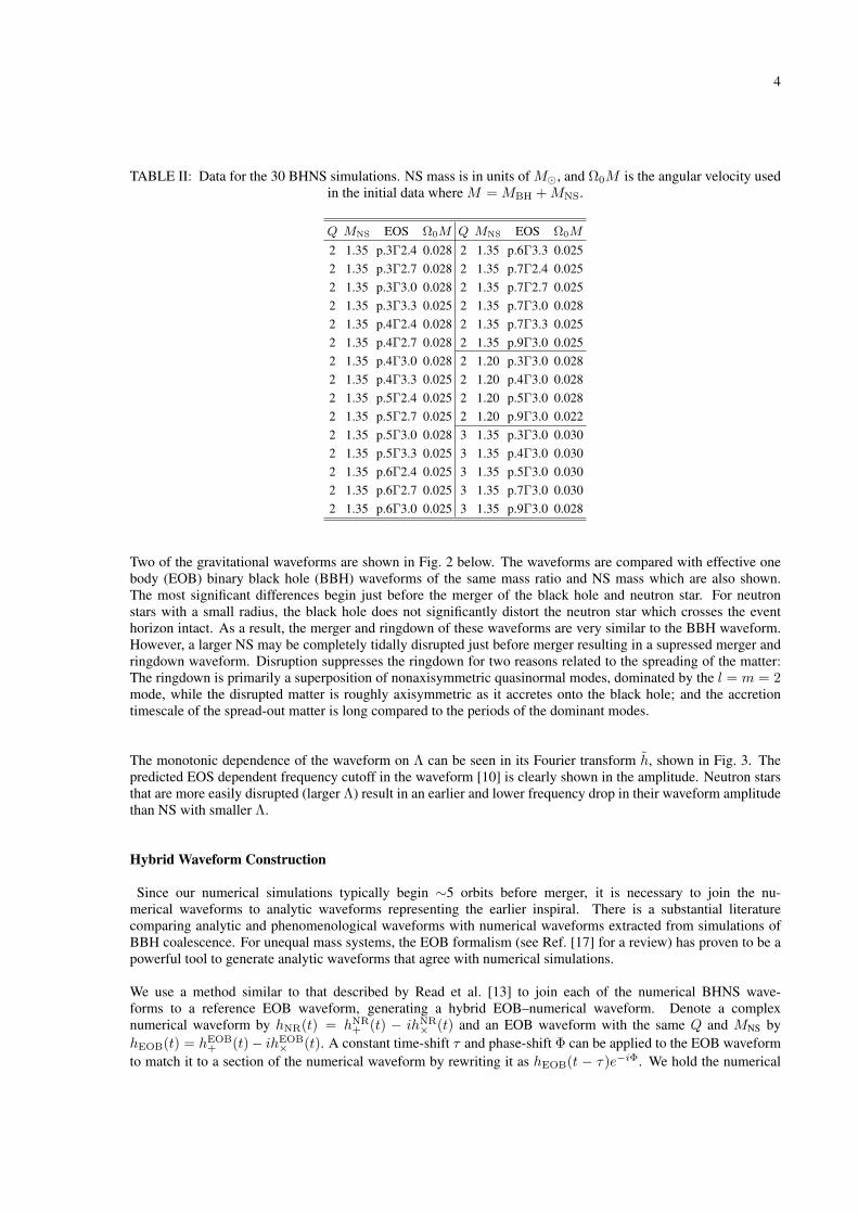
TABLE II: Data for the 30 BHNS simulations. NS mass is in units of M, and Ω0M is the angular velocity usedin the initial data where M = MBH +MNS.

Q MNS EOS Ω0M Q MNS EOS Ω0M

2 1.35 p.3Γ2.4 0.028 2 1.35 p.6Γ3.3 0.0252 1.35 p.3Γ2.7 0.028 2 1.35 p.7Γ2.4 0.0252 1.35 p.3Γ3.0 0.028 2 1.35 p.7Γ2.7 0.0252 1.35 p.3Γ3.3 0.025 2 1.35 p.7Γ3.0 0.0282 1.35 p.4Γ2.4 0.028 2 1.35 p.7Γ3.3 0.0252 1.35 p.4Γ2.7 0.028 2 1.35 p.9Γ3.0 0.0252 1.35 p.4Γ3.0 0.028 2 1.20 p.3Γ3.0 0.0282 1.35 p.4Γ3.3 0.025 2 1.20 p.4Γ3.0 0.0282 1.35 p.5Γ2.4 0.025 2 1.20 p.5Γ3.0 0.0282 1.35 p.5Γ2.7 0.025 2 1.20 p.9Γ3.0 0.0222 1.35 p.5Γ3.0 0.028 3 1.35 p.3Γ3.0 0.0302 1.35 p.5Γ3.3 0.025 3 1.35 p.4Γ3.0 0.0302 1.35 p.6Γ2.4 0.025 3 1.35 p.5Γ3.0 0.0302 1.35 p.6Γ2.7 0.025 3 1.35 p.7Γ3.0 0.0302 1.35 p.6Γ3.0 0.025 3 1.35 p.9Γ3.0 0.028

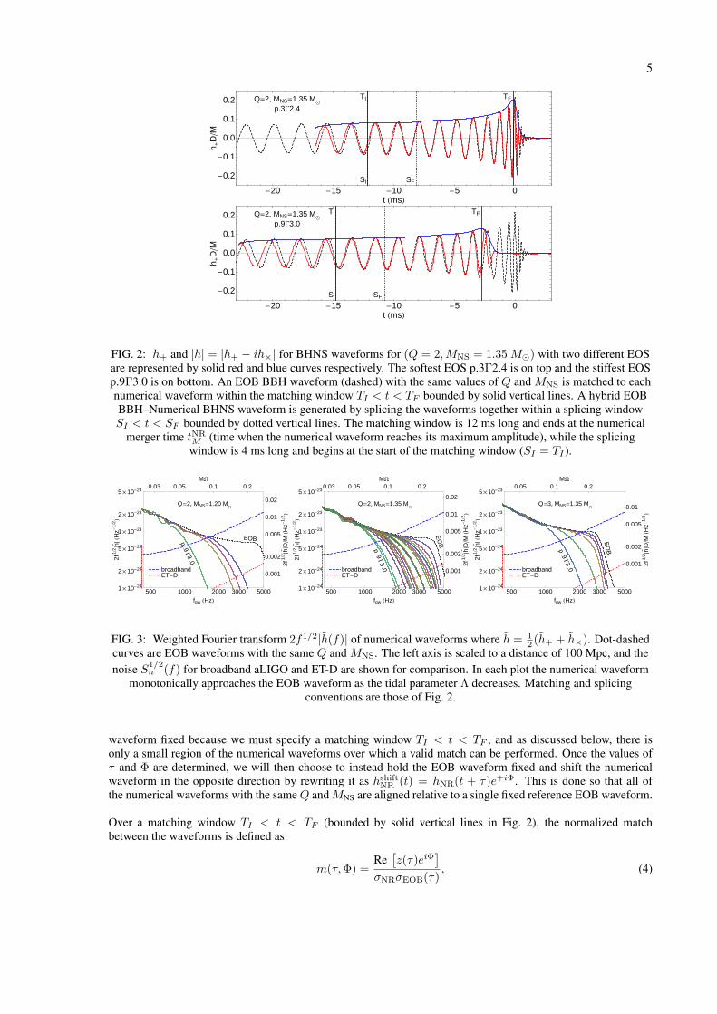
Two of the gravitational waveforms are shown in Fig. 2 below. The waveforms are compared with effective onebody (EOB) binary black hole (BBH) waveforms of the same mass ratio and NS mass which are also shown.The most significant differences begin just before the merger of the black hole and neutron star. For neutronstars with a small radius, the black hole does not significantly distort the neutron star which crosses the eventhorizon intact. As a result, the merger and ringdown of these waveforms are very similar to the BBH waveform.However, a larger NS may be completely tidally disrupted just before merger resulting in a supressed merger andringdown waveform. Disruption suppresses the ringdown for two reasons related to the spreading of the matter:The ringdown is primarily a superposition of nonaxisymmetric quasinormal modes, dominated by the l = m = 2mode, while the disrupted matter is roughly axisymmetric as it accretes onto the black hole; and the accretiontimescale of the spread-out matter is long compared to the periods of the dominant modes.

The monotonic dependence of the waveform on Λ can be seen in its Fourier transform h, shown in Fig. 3. Thepredicted EOS dependent frequency cutoff in the waveform [10] is clearly shown in the amplitude. Neutron starsthat are more easily disrupted (larger Λ) result in an earlier and lower frequency drop in their waveform amplitudethan NS with smaller Λ.

Hybrid Waveform Construction

Since our numerical simulations typically begin ∼5 orbits before merger, it is necessary to join the nu-merical waveforms to analytic waveforms representing the earlier inspiral. There is a substantial literaturecomparing analytic and phenomenological waveforms with numerical waveforms extracted from simulations ofBBH coalescence. For unequal mass systems, the EOB formalism (see Ref. [17] for a review) has proven to be apowerful tool to generate analytic waveforms that agree with numerical simulations.

We use a method similar to that described by Read et al. [13] to join each of the numerical BHNS wave-forms to a reference EOB waveform, generating a hybrid EOB–numerical waveform. Denote a complexnumerical waveform by hNR(t) = hNR

+ (t) − ihNR× (t) and an EOB waveform with the same Q and MNS by

hEOB(t) = hEOB+ (t)− ihEOB

× (t). A constant time-shift τ and phase-shift Φ can be applied to the EOB waveformto match it to a section of the numerical waveform by rewriting it as hEOB(t − τ)e−iΦ. We hold the numerical

5

Q=2, MNS=1.35 M

p.3G2.4

TI TF

SI SF

-20 -15 -10 -5 0

-0.2

-0.1

0.0

0.1

0.2

t HmsLh +

DM

Q=2, MNS=1.35 M

p.9G3.0

TI TF

SI SF

-20 -15 -10 -5 0

-0.2

-0.1

0.0

0.1

0.2

t HmsL

h +D

M

FIG. 2: h+ and |h| = |h+ − ih×| for BHNS waveforms for (Q = 2,MNS = 1.35 M) with two different EOSare represented by solid red and blue curves respectively. The softest EOS p.3Γ2.4 is on top and the stiffest EOSp.9Γ3.0 is on bottom. An EOB BBH waveform (dashed) with the same values of Q and MNS is matched to eachnumerical waveform within the matching window TI < t < TF bounded by solid vertical lines. A hybrid EOBBBH–Numerical BHNS waveform is generated by splicing the waveforms together within a splicing windowSI < t < SF bounded by dotted vertical lines. The matching window is 12 ms long and ends at the numerical

merger time tNRM (time when the numerical waveform reaches its maximum amplitude), while the splicingwindow is 4 ms long and begins at the start of the matching window (SI = TI ).

broadbandET-D

500 1000 2000 3000 50001 ´ 10-24

2 ´ 10-24

5 ´ 10-24

1 ´ 10-23

2 ´ 10-23

5 ´ 10-230.03 0.05 0.1 0.2

0.001

0.002

0.005

0.01

0.02

fgw HHzL

2f12

Èh ÈHHz-

12L

MW

2f12

Èh ÈDMHHz

-12

L

Q=2, MNS=1.20 M

p .9

G3 .0

EOB

broadbandET-D

500 1000 2000 3000 50001 ´ 10-24

2 ´ 10-24

5 ´ 10-24

1 ´ 10-23

2 ´ 10-23

5 ´ 10-230.03 0.05 0.1 0.2

0.001

0.002

0.005

0.01

0.02

fgw HHzL

2f12

Èh ÈHHz-

12L

MW

2f12

Èh ÈDMHHz

-12

L

Q=2, MNS=1.35 M

p .9

G3 .0

EO

B

broadbandET-D

500 1000 2000 3000 50001 ´ 10-24

2 ´ 10-24

5 ´ 10-24

1 ´ 10-23

2 ´ 10-23

5 ´ 10-230.05 0.1 0.2

0.001

0.002

0.005

0.01

fgw HHzL

2f12

Èh ÈHHz-

12L

MW

2f12

Èh ÈDMHHz

-12

L

Q=3, MNS=1.35 M

p .9

G3 .0

EO

B

FIG. 3: Weighted Fourier transform 2f1/2|h(f)| of numerical waveforms where h = 12 (h+ + h×). Dot-dashed

curves are EOB waveforms with the same Q and MNS. The left axis is scaled to a distance of 100 Mpc, and thenoise S1/2

n (f) for broadband aLIGO and ET-D are shown for comparison. In each plot the numerical waveformmonotonically approaches the EOB waveform as the tidal parameter Λ decreases. Matching and splicing

conventions are those of Fig. 2.

waveform fixed because we must specify a matching window TI < t < TF , and as discussed below, there isonly a small region of the numerical waveforms over which a valid match can be performed. Once the values ofτ and Φ are determined, we will then choose to instead hold the EOB waveform fixed and shift the numericalwaveform in the opposite direction by rewriting it as hshift

NR (t) = hNR(t + τ)e+iΦ. This is done so that all ofthe numerical waveforms with the sameQ andMNS are aligned relative to a single fixed reference EOB waveform.

Over a matching window TI < t < TF (bounded by solid vertical lines in Fig. 2), the normalized matchbetween the waveforms is defined as

m(τ,Φ) =Re[z(τ)eiΦ

]σNRσEOB(τ)

, (4)

6

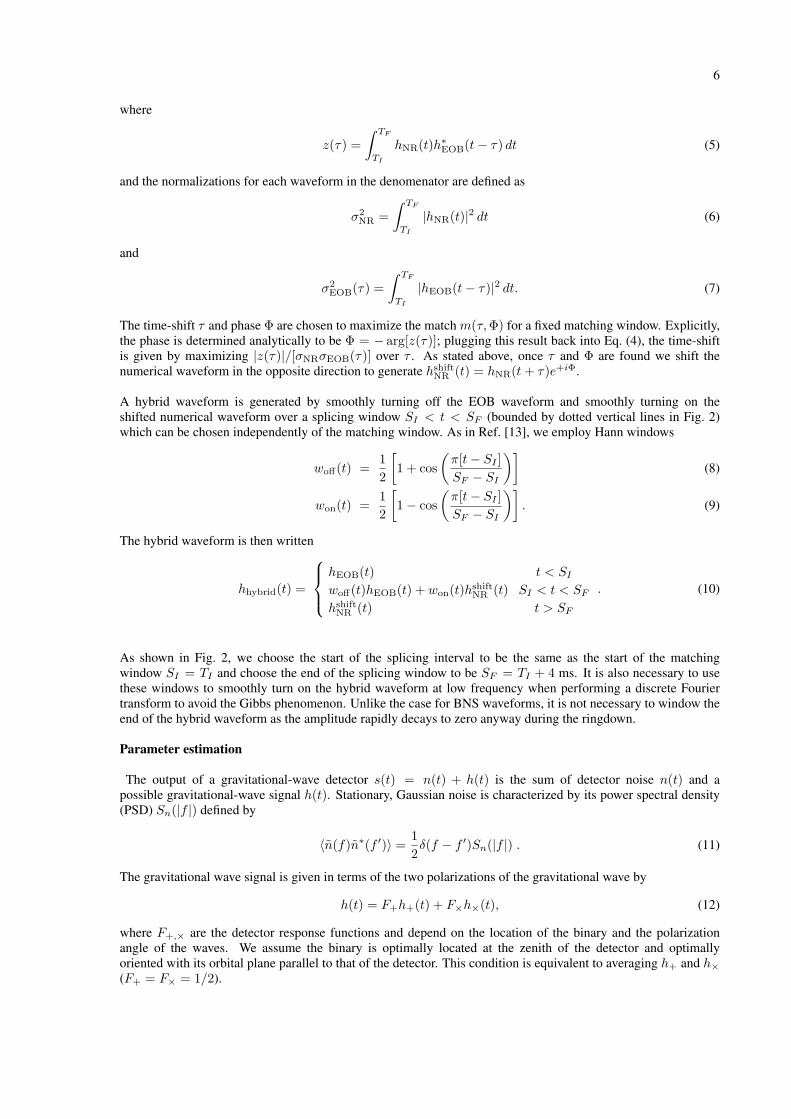
where

z(τ) =∫ TF

TI

hNR(t)h∗EOB(t− τ) dt (5)

and the normalizations for each waveform in the denomenator are defined as

σ2NR =

∫ TF

TI

|hNR(t)|2 dt (6)

and

σ2EOB(τ) =

∫ TF

TI

|hEOB(t− τ)|2 dt. (7)

The time-shift τ and phase Φ are chosen to maximize the match m(τ,Φ) for a fixed matching window. Explicitly,the phase is determined analytically to be Φ = − arg[z(τ)]; plugging this result back into Eq. (4), the time-shiftis given by maximizing |z(τ)|/[σNRσEOB(τ)] over τ . As stated above, once τ and Φ are found we shift thenumerical waveform in the opposite direction to generate hshift

NR (t) = hNR(t+ τ)e+iΦ.

A hybrid waveform is generated by smoothly turning off the EOB waveform and smoothly turning on theshifted numerical waveform over a splicing window SI < t < SF (bounded by dotted vertical lines in Fig. 2)which can be chosen independently of the matching window. As in Ref. [13], we employ Hann windows

woff(t) =12

[1 + cos

(π[t− SI ]SF − SI

)](8)

won(t) =12

[1− cos

(π[t− SI ]SF − SI

)]. (9)

The hybrid waveform is then written

hhybrid(t) =

hEOB(t) t < SIwoff(t)hEOB(t) + won(t)hshift

NR (t) SI < t < SFhshift

NR (t) t > SF

. (10)

As shown in Fig. 2, we choose the start of the splicing interval to be the same as the start of the matchingwindow SI = TI and choose the end of the splicing window to be SF = TI + 4 ms. It is also necessary to usethese windows to smoothly turn on the hybrid waveform at low frequency when performing a discrete Fouriertransform to avoid the Gibbs phenomenon. Unlike the case for BNS waveforms, it is not necessary to window theend of the hybrid waveform as the amplitude rapidly decays to zero anyway during the ringdown.

Parameter estimation

The output of a gravitational-wave detector s(t) = n(t) + h(t) is the sum of detector noise n(t) and apossible gravitational-wave signal h(t). Stationary, Gaussian noise is characterized by its power spectral density(PSD) Sn(|f |) defined by

〈n(f)n∗(f ′)〉 =12δ(f − f ′)Sn(|f |) . (11)

The gravitational wave signal is given in terms of the two polarizations of the gravitational wave by

h(t) = F+h+(t) + F×h×(t), (12)

where F+,× are the detector response functions and depend on the location of the binary and the polarizationangle of the waves. We assume the binary is optimally located at the zenith of the detector and optimallyoriented with its orbital plane parallel to that of the detector. This condition is equivalent to averaging h+ and h×(F+ = F× = 1/2).

7

It is well known [18] that the optimal statistic for detection of a known signal h(t) in additive Gaussiannoise is

ρ =(h|s)√(h|h)

(13)

where the inner product between two signals h1 and h2 is given by

(h1|h2) = 4Re∫ ∞

0

h1(f)h∗2(f)Sn(f)

df. (14)

In searches for gravitational-wave signals from compact binary mergers, a parametrized signal h(t; θA) is knownin advance of detection, and the parameters θA must be estimated from the measured detector output s(t). Theparameters θA of an inspiral are estimated by maximizing the inner product of the signal s(t) over the templatewaveforms h(t; θA). In the high signal-to-noise limit, the statistical uncertainty in the estimated parameters θA

arising from the instrumental noise can be estimated using the Fisher matrix

ΓAB =(∂h

∂θA

∣∣∣∣ ∂h∂θB)∣∣∣∣

θA

. (15)

Note that θA are the parameter values that maximize the signal-to-noise. The variance σ2A = σAA = 〈(∆θA)2〉

and covariance σAB = 〈∆θA∆θB〉 of the parameters are then given in terms of the Fisher matrix by

〈∆θA∆θB〉 = (Γ−1)AB . (16)

For hybrid waveforms, the partial derivatives in the Fisher matrix must be approximated with finite differ-ences. It is most robust to compute the derivatives of the Fourier transforms used in the inner product. Werewrite the Fourier transform of each waveform in terms of the amplitude A and phase Φ as exp[lnA− iΦ]. Thederivatives ∂ lnA/∂θA and ∂Φ/∂θA are then evaluated with finite differencing.

In general, errors in the parameters θA are correlated with each other forming an error ellipsoid in param-eter space determined by the Fisher matrix ΓAB . The uncorrelated parameters that are best extracted from thesignal are found by diagonalizing ΓAB . These new parameters are linear combinations of the original parametersθA. We focus attention below on the two parameters log(p1) and Γ, and fix all other parameters. We thereforeconstruct the error ellipses in log(p1),Γ parameter space and identify the parameter with the smallest statisticalerrors.

For the BHNS systems discussed here, the greatest departure from BBH behavior occurs for gravitational-wave frequencies in the range 500–5000 Hz. As a result, detector configurations optimized for detection of BHNSsystems with low noise in the region below 500 Hz are not ideal for estimating EOS parameters. We thereforepresent results for the broadband aLIGO noise curve [19] and the ET-D noise curve [20] shown in Fig. 4.

In Fig. 5, we show the resulting 1-σ error ellipses in the 2-dimensional parameter space log(p1),Γ for anoptimally oriented BHNS with Q = 2 and MNS = 1.35M at a distance of 100 Mpc. Surfaces of constantΛ1/5 and NS radius, which are almost parallel to each other, are also shown. One can see that the error ellipsesare aligned with these surfaces. This indicates that, as expected, Λ1/5 is the parameter that is best extractedfrom BHNS gravitational-wave observations. Because Λ1/5 and R are so closely aligned we will use these twoparameters interchangeably.

As mentioned above, there is some freedom in construction of the hybrid waveforms. The size and orientation ofthe error ellipses also depend on the details of this construction. We find that as long as the matching window islonger than approximately four gravitational-wave cycles to average out the effects of eccentricity and does notinclude the first two gravitational-wave cycles, the orientation of the error ellipses does not change significantly.As expected, the size of the ellipses decreases as more of the numerical waveform is incorporated into the hybrid

8

narrowbandbroadbandET-D

10 50 100 500 1000 50001 ´ 10-25

5 ´ 10-25

1 ´ 10-24

5 ´ 10-24

1 ´ 10-23

5 ´ 10-23

1 ´ 10-22

f HHzLS

h1

2HH

z-1

2L

fR

fR

fR

FIG. 4: Noise PSD for broadband aLIGO (dashed blue), ET-D (dotted red) and various configurations ofnarrowband aLIGO (solid black). The minima of the narrowband configuration are labeled fR

´

´

´

´

´

´

´

2.0 2.5 3.0 3.5 4.034.0

34.2

34.4

34.6

34.8

35.0

G

logH

p 1L@

dyne

cm2

D

L 15=3.0

L15 =4.0

L15 =5.0

´

´

´

´

´

´

´

2.0 2.5 3.0 3.5 4.034.0

34.2

34.4

34.6

34.8

35.0

G

logH

p 1L@

dyne

cm2

D

R=10 km

R=12 km

R=14 kmR=16 km

FIG. 5: 1–σ error ellipses for ET-D. Evenly spaced contours of constant Λ1/5 (R) are also shown on the left(right). Matching and splicing conventions are those of Fig. 2.

waveform. We therefore adopt the last 12 ms before merger of each numerical waveform as the matching windowand the first 4 ms of the matching window for splicing as shown in Fig. 2.

We have emphasized that, to within present numerical accuracy, the late-inspiral waveform is determinedby the single parameter Λ1/5. This implies that, by using countours of constant Λ in the EOS space, one couldhave obtained the constraint on the EOS, summarized in Fig. 5 by varying only a single EOS parameter. For thesimulations with other mass ratios and neutron star masses, we have used as our single parameter log(p1) and notΓ because countours of constant p1 more closely coincide with contours of constant Λ and because Λ is a one toone function of log(p1) throughout the parameter space. The one-parameter Fisher matrix can then be evaluatedwith finite differencing using the waveforms and values of Λ at two points in EOS parameter space with differentlog(p1).

The uncertainties in Λ1/5 and R are shown in Fig. 6 for broadband aLIGO. The uncertainty in these quan-tities is ∼ 10–40% for broadband aLIGO and are shifted down by an order of magnitude to ∼ 1–4% for ET-D.The uncertainties for the higher mass ratio Q = 3 are somewhat larger than for Q = 2, but not significantly so.It is not clear how rapidly the uncertainty in Λ1/5 and R will increase as the mass ratio is increased toward morerealistic values. On the one hand the tidal distortion is likely to be much smaller for larger Q. On the other handthe overall signal will be louder, and the merger and ringdown will occur at lower frequencies where the noise islower. Additional simulations for higher Q are needed to address this question.

9

ò ò

ò

á

áá

á

áááá ááá

ááááá

ø

ø

ø

ò Q=2, MNS=1.20M

á Q=2, MNS=1.35M

ø Q=3, MNS=1.35M

2.5 3.0 3.5 4.0 4.5 5.00.0

0.5

1.0

1.5

2.0

L15

ΣL

15

ò ò

ò

á

á

áá

áá

áá ááá

á

áááá

ø

ø

ø

ò Q=2, MNS=1.20M

á Q=2, MNS=1.35M

ø Q=3, MNS=1.35M

10 11 12 13 14 15 160

1

2

3

4

5

R HkmL

ΣR

HkmL

FIG. 6: 1-σ uncertainty σΛ1/5 and σR as a function of the parameters Λ1/5 or R for the broadband aLIGO noisePSD. Matching and splicing conventions are those of Fig. 2.

The presence of a signal-recycling cavity in the aLIGO instruments will allow them to be tuned to have improvednarrowband sensitivity at the expense of bandwith. We have examined several narrowband tunings with centralfrequencies that vary between approximately fR = 500 Hz and 4000 Hz. Three of these noise curves areshown in Fig. 4. In Fig. 7 we plot the 1–σ uncertainty in NS radius σR as a function of the narrowband centralfrequency fR. For the waveforms considered in this paper the optimal narrowband frequency is in the range1000 Hz . fR . 2500 Hz and depends on the mass ratio, NS mass, and EOS. Narrowband configurations usuallygive smaller errors than the broadband configuration if fR happens to be tuned to within a few hundred Hz of theminimum for that BHNS event.

R=11.3km Hp.35G3.0LR=11.9km Hp.45G3.0LR=13.6km Hp.7G3.0L

0 1000 2000 3000 40000

1

2

3

4

5

Narrowband central frequency fR HHzL

ΣR

HkmL

Q=2, MNS=1.20 M

broad

ET-D

R=11.3km Hp.35G3.0LR=11.9km Hp.45G3.0LR=13.3km Hp.65G3.0LR=14.4km Hp.8G3.0L

0 1000 2000 3000 40000

1

2

3

4

5

Narrowband central frequency fR HHzL

ΣR

HkmL

Q=2, MNS=1.35 M

broad

ET-DR=11.6km Hp.4G3.0LR=12.9km Hp.6G3.0LR=14.4km Hp.8G3.0L

0 1000 2000 3000 40000

1

2

3

4

5

Narrowband central frequency fR HHzL

ΣR

HkmL

Q=3, MNS=1.35 Mbroad

ET-D

FIG. 7: 1–σ uncertainty in R for different configurations of narrowband aLIGO and for different EOS. fRdefines the frequency where Sn is a minimum as shown in Fig. 4. Horizontal lines on the left and right indicatethe corresponding 1–σ errors for broadband aLIGO and ET-D respectively. Matching and splicing conventions

are those of Fig. 2.

Discussion

Using a large set of simulations incorporating a two-parameter EOS, we have found that the tidal de-formability Λ1/5, or equivalently the NS radius R, is the parameter that will be best extracted from BHNSwaveforms. These parameters can be estimated to 10–40% with broadband aLIGO for an optimally orientedBHNS binary at 100 Mpc. The narrowband aLIGO configuration can do slightly better if it is tuned to within afew hundred Hz of the ideal frequency for a given BHNS event. The proposed Einstein Telescope will have anorder-of-magnitude better sensitivity to the EOS parameters.

The results presented here can be compared with recent work to determine the mass and radius of individual NSin Type-1 X-ray bursts. Ozel et al. [21] have obtained mass and radius measurements from several systems bysimultaneously measuring the flux F , which is likely close to the Eddington value, and the blackbody temperatureT during X-ray bursts of systems with accurately determined distances. They obtain estimates of NS mass and

10

radii with O(10%) 1–σ uncertainty. These radius error estimates are slightly smaller than those for the BHNSsystems we have considered at 100 Mpc. However, we note that binary inspiral observations are subject to lesssystematic uncertainty due to questions of composition of the photosphere and associating it with the NS surface.

The uncertainty in NS radius for the merger and ringdown of BHNS systems examined here is of roughlythe same size as that found for the last few orbits up to merger of BNS systems at the same 100 Mpc dis-tance [13, 22]. BNS inspirals, however, will likely occur more frequently, and, including a tidally correctedinspiral–numerical hybrid, BNS systems are likely to have uncertainties that are smaller than BHNS systems by afactor of a few. Considering the post-merger phase for BNS waveforms may also provide additional information.Expected NS masses in both BNS and BHNS systems are slightly smaller than those measured for X-ray bursterswhich have accreted matter from their companion, so BNS and BHNS GW observations may complement X-rayburst observations by better constraining the lower density range of the EOS which is not well constained fromX-ray burst observations [21, 23].

[1] J. Abadie, B. P. Abbott, R. Abbott, M. Abernathy, T. Accadia, F. Acernese, C. Adams, R. Adhikari, P. Ajith, B. Allen,et al., Classical and Quantum Gravity 27, 173001 (2010), 1003.2480.

[2] K. Belczynski, M. Dominik, T. Bulik, R. O’Shaughnessy, C. Fryer, and D. E. Holz, 715, L138 (2010), 1004.0386.[3] K. Belczynski, V. Kalogera, and T. Bulik, Astrophys. J. 572, 407 (2002), arXiv:astro-ph/0111452.[4] T. Hinderer, Astrophys. J. 677, 1216 (2008), 0711.2420.[5] E. E. Flanagan and T. Hinderer, Phys. Rev. D 77, 021502 (2008), 0709.1915.[6] J. Vines and E. E. Flanagan, ArXiv e-prints (2010), 1009.4919.[7] J. Vines, T. Hinderer, and E. E. Flanagan, ArXiv e-prints (2011), 1101.1673.[8] T. Damour and A. Nagar, Phys. Rev. D 80, 084035 (2009), 0906.0096.[9] T. Binnington and E. Poisson, Phys. Rev. D 80, 084018 (2009), 0906.1366.

[10] M. Vallisneri, Physical Review Letters 84, 3519 (2000), arXiv:gr-qc/9912026.[11] J. S. Read, B. D. Lackey, B. J. Owen, and J. L. Friedman, Phys. Rev. D 79, 124032 (2009), 0812.2163.[12] J. M. Lattimer and M. Prakash, Astrophys. J. 550, 426 (2001), arXiv:astro-ph/0002232.[13] J. S. Read, C. Markakis, M. Shibata, K. Uryu, J. D. E. Creighton, and J. L. Friedman, Phys. Rev. D 79, 124033 (2009),

0901.3258.[14] K. Kyutoku, M. Shibata, and K. Taniguchi, Phys. Rev. D 82, 044049 (2010), 1008.1460.[15] K. Kyutoku, H. Okawa, M. Shibata, and K. Taniguchi, ArXiv e-prints (2011), 1108.1189.[16] P. B. Demorest, T. Pennucci, S. M. Ransom, M. S. E. Roberts, and J. W. T. Hessels, Nature (London) 467, 1081 (2010),

1010.5788.[17] T. Damour and A. Nagar, ArXiv e-prints (2009), 0906.1769.[18] L. A. Wainstein and V. D. Zubakov, Extraction of signals from noise (Prentice-Hall, Englewood Cliffs, NJ, 1962).[19] D. Shoemaker (LSC, 2009), URL https://dcc.ligo.org/cgi-bin/DocDB/ShowDocument?docid=

2974.[20] S. Hild, M. Abernathy, F. Acernese, P. Amaro-Seoane, N. Andersson, K. Arun, F. Barone, B. Barr, M. Barsuglia,

M. Beker, et al., Classical and Quantum Gravity 28, 094013 (2011), 1012.0908.[21] F. Ozel, G. Baym, and T. Guver, Phys. Rev. D 82, 101301 (2010), 1002.3153.[22] L. Baiotti, J. Creighton, B. Giacomazzo, K. Kyutoku, C. Markakis, J. Read, L. Rezzolla, M. Shibata, K. Taniguchi, and

J. Friedman, in progress (2011).[23] F. Ozel and D. Psaltis, Phys. Rev. D 80, 103003 (2009).[24] The tidal deformability for the `th multipole is often defined in terms of the NS radius R and its dimensionless `th Love

number k` by λ` = 2(2`−1)!!G

k`R2`+1. Here we will discuss only the ` = 2 term so we write λ := λ2.