Externalities and Benefit Design in Health Insurance

Amanda Starc

Kellogg School of Management, Northwestern University and NBER

Robert J. Town∗

University of Texas - Austin and NBER

May 2019

Abstract

Insurance benefit design has important implications for consumer welfare. In this paper, we model insurer be-

havior in the Medicare prescription drug coverage market and show that strategic private insurer incentives impose

a fiscal externality on the traditional Medicare program. We document that plans covering medical expenses have

more generous drug coverage than plans that are only responsible for prescription drug spending, which translates

into higher drug utilization by enrollees. The effect is driven by drugs that reduce medical expenditure and treat

chronic conditions. Our equilibrium model of benefit design endogenizes plan characteristics and accounts for asym-

metric information; the model estimates confirm that differential incentives to internalize medical care offsets can

explain disparities across plans. Counterfactuals show that strategic insurer incentives are as important as asymmetric

information in determining benefit design.

∗Kellogg School of Management, 2001 Sheridan Road, Evanston, IL, and Department of Economics, The University of Texas at Austin, 2225Speedway, Austin, TX. The authors gratefully acknowledge funding from the Leonard Davis Institute. Meghan Busse, David Dranove, MichaelFrench, Josh Gottleib, Matt Grennan, Ben Handel, Jonathan Ketcham, Kurt Lavetti, Maria Polyakova, Joshua Schwartzstein, Ashley Swanson, andparticipants at the American Health Economics Conference, FTC Microeconomics Conference, NBER Insurance Meetings, Kellogg HealthcareMarkets Conference, Wharton IO lunch, University of British Columbia, Indiana University, University of Chicago, and Yale provided helpfulcomments. Hossein Alidaee, Emma Boswell Dean, Jordan Keener, Victoria Marone, and David Stillerman provided excellent research assistance.The authors thank the editor and four anonymous referees for their thoughtful comments.

1

1 Introduction

The welfare generated by private health insurance critically depends on the structure of benefits offered by insurers.

More generous benefits provide increased enrollee risk protection but are costly to the risk-bearing insurer. Increasing

generosity mechanically increases plan expenditures and, more important from a welfare perspective, increases the

likelihood of moral hazard and adverse selection. An optimal insurance plan must balance these gains from risk

protection against inefficiencies due to asymmetric information.

While this theoretical trade-off is well-understood, most recent empirical models of equilibrium insurer behavior

focus exclusively on the pricing behavior of insurers holding benefit design fixed (Handel (2013); Starc (2015); Town

and Liu (2003); Tebaldi (2017); Ericson and Starc (2015); Decarolis, Polyakova and Ryan (Forthcoming)). The litera-

ture highlights the important role of imperfect competition and strategic insurer behavior – in addition to asymmetric

information – in driving equilibrium outcomes. In this paper, we develop and estimate a tractable oligopoly model

of premium setting and benefit design. We use our model to quantify the impact of both asymmetric information

and strategic incentives on premium setting and benefit design. To study the role of insurers’ strategic incentives in

shaping benefit design, we examine the impact of an important friction in benefit design in our setting: externalities

due to incentive misalignment. We find that this externality plays as important of a role as asymmetric information in

affecting equilibrium plan benefit design.

Patient care often spans different treatment modalities (e.g., inpatient, office visits, outpatient surgery, specialist

care, pharmaceuticals), and coverage for one type of care may interact and spill over to other services, creating the

potential for an externality (Goldman and Philipson (2007); McGuire (2011); Goldman, Joyce and Zheng (2007)). We

focus on the classic example of drug offsets: a substantial body of evidence shows that more generous drug coverage

increases drug adherence, preventing future inpatient utilization. Unless insurers are responsible for coverage across

linked treatment modalities, they will have limited incentives to internalize this externality in their benefit design

decisions. The welfare impact of these benefit design decisions are potentially large, as the level and composition

of consumption of health care services depend on insurer benefit design. We model the benefit design decisions of

insurers and estimate the impact of this externality by studying the mandated separation of covered benefits categories

for private insurers providing services in the United States Medicare system in Medicare Part D.

The Medicare Part D program provides prescription drug coverage to beneficiaries through private plans that

are publicly financed. In 2015, over 39 million Medicare beneficiaries signed up for a Part D plan, accounting for

$137 billion in drug spending. Under the Medicare Part D program, there are two major categories of drug plans:

stand-alone prescription drug plans (PDPs) and Medicare Advantage Prescription Drug (MA-PD) plans. Stand-alone

PDPs are mandated to cover only pharmaceutical expenditures, while MA-PD plans cover both drug and medical

expenditures. These differences imply that the two types of plans face different benefit design incentives. Stand-alone

2

PDPs have an incentive to minimize drug expenditures, ignoring the impact on medical spending, while MA-PD plans

have an incentive to minimize overall medical and drug expenditures, taking externalities from drug consumption to

medical care utilization into account. As a result, MA-PD plans have an incentive to provide more generous coverage

for drugs – particularly for those drugs for which increased adherence reduces medical expenditures.

Our primary data source is the rich Medicare Part D prescription drug claims data. We observe every prescription

fill for the years 2006-2009 for a random 10% sample of all Medicare eligibles. These data contain information on

the specific drug filled, retail price, enrollee out-of-pocket cost, and fill date for over 123 million drug claim events.

We supplement claims data with information on beneficiary and plan characteristics. The beneficiary data contain

information on enrollee demographics and the plan enrollment details. The plan data contain detailed information on

the premiums and benefit design (e.g., which drugs are on each benefit tier and the coinsurance/co-payment structures

of each tier).

We begin the empirical analysis by comparing the benefit designs of PDPs and MA-PD plans. The comparison is

challenging because there are over 35,000 unique pharmaceutical products for which plans need to determine coverage,

and plans generally employ a complex nonlinear plan design. Over our sample period, the Part D standard benefit

package included a deductible, an initial coverage region where enrollee costs are limited, the donut hole where the

enrollee is responsible for 100% of the cost of their drugs, and finally the catastrophic region where the enrollee

is responsible for only a small fraction of drug cost. Using the detailed prescription level data with over 123 million

claims, we estimate that MA-PD plan enrollees spend between 8 and 11 percent less on average for an identical bundle

of drugs. The differences across plan type are larger for sicker enrollees. Furthermore, consistent with externalities

playing a key role, the expenditure differentials are largely driven by drugs that have been explicitly identified as

having large medical care offsets and treat chronic conditions like asthma, diabetes, and high cholesterol.

We then turn to the main empirical exercise: specifying and estimating the structural parameters of an oligopoly

model of premium and benefit design choice. To capture insurer incentives, we model both consumer plan choice and

insurer benefit design. Importantly, the model allows for drug expenditures and preferences to vary across consumers,

and captures the extent to which differences in generosity by plan type can be rationalized by consumer demand and

asymmetric information. We also allow strategic insurer incentives to vary by plan type. The model recovers cost and

demand side parameters, enabling us to understand the economic rationale behind increased prescription drug benefit

generosity in MA-PD plans. Consistent with previous work, the demand side estimates imply that consumer respon-

siveness to plan generosity when choosing plans is modest. Consistent with the importance of offsets, the supply side

estimates show that MA-PD plans find it less costly to increase generosity than their stand-alone counterparts. Taken

together, the model parameters imply that the increased generosity of MA-PD plans is driven by both asymmetric

information and insurer cost side incentives.

Using the model and parameter estimates, we measure the impact of various economic forces on benefit design,

3

including the effect of plans internalizing the externalities generated by offsets. We find substantial medical care

offsets in MA-PD plans: a $1 increase in prescription drug spending reduces non-drug expenditure by approximately

27 cents.1 If stand-alone PDPs were forced to account for this externality in their premiums and benefit design

behavior, insurer drug spending would increase by 7%. Based on these estimates, we find that stand-alone PDPs

impose a $378 million externality (-.8% of Part D spending) on traditional Medicare each year.

In addition to explicitly modeling incentives to internalize offsets, the model allows for and explores the impact

of asymmetric information. Specifically, we account for selection and screening incentives (Geruso, Layton and

Prinz (Forthcoming); Carey (2017); Lavetti and Simon (2018)) and moral hazard (Einav, Finkelstein and Polyakova

(2016)).2 Critically, we show that asymmetric information also has an impact on benefit design: absent selection and

moral hazard, insurer drug spending would increase by an additional 7%. In contrast to a large literature focused on the

dead-weight loss due to moral hazard and over-consumption of medical services, our paper finds evidence of potential

under-consumption. Our analysis further shows that strategic incentives are equally important determinants of benefit

design. Given market imperfections, benefit design in both MA-PD and stand-alone PDPs is unlikely to be socially

optimal. However, our approach helps us better understand insurer incentives, explore the implications of endogenous

product benefit design in the Medicare Part D marke, and provide a framework for future researchers.

Our work also expands on the recent literature examining insurer competition in private Medicare markets (e.g.

Decarolis, Polyakova and Ryan (Forthcoming); Curto et al. (2015)); more broadly, we contribute to a recent, growing

literature on endogenous product design (see Fan (2013) and Crawford (2012) for a review).3 The paper is organized

as follows. Section 2 describes the market. Section 3 presents the reduced form estimations. Section 4 describes and

estimates our model of firm behavior. Section 5 presents counterfactual exercises that put the magnitude of our effect

in context, and Section 6 concludes.

2 Empirical Setting and Data

In this section, we describe the role of private insurers within Medicare, which provides health insurance to the elderly

in the United States.4 Private insurers play an important role in administering benefits; as a result, our setting is a data

1These offsets of medical care costs are viewed as sufficiently important to be included in government budget forecasts of health care expendi-tures, and are consistent with previous estimates. This estimate aligns with previous work by Chandra, Gruber and McKnight (2010), who examineoffsets using demand-side consumption. We cannot employ a similar strategy because we do not observe medical claims for enrollees in MA-PDplans.

2We also explore the impact of behavioral biases including inertia (Ho, Hogan and Scott Morton (2015); Polyakova (2016)), and explore theimpact of choice frictions and the under-utilization of cost-effective care (Abaluck and Gruber (2011); Ketcham et al. (2012)) and Manning et al.(1987), Brot-Goldberg et al. (2017)). Critically, our modeling approach accounts for imperfect competition among insurers (Decarolis, Polyakovaand Ryan (Forthcoming)) and extends existing models that endogenize prices but hold product characteristics fixed (Handel (2013); Lustig (2010);Starc (2015); Town and Liu (2003); Tebaldi (2017); Ericson and Starc (2015)).

3Fan (2013) is the closest to our setting, as she explores continuous quality attributes. See also Draganska, Mazzeo and Seim (2009); Eizenberg(2014); Sweeting (2010); Wollman (2018).

4Medicare also provides health insurance coverage for the disabled and those with End Stage Renal Disease. We do not focus on those popula-tions in this paper.

4

rich – if institutionally complex – laboratory in which to explore endogenous product design. Medicare Parts A and

B are publicly administered and cover inpatient and outpatient services, respectively. Medicare Advantage (Part C)

and Part D are administered by private insurers. Medicare Advantage is an alternative to traditional Medicare under

Parts A and B, and Medicare Part D covers prescription drugs. Under both Medicare Advantage and Part D, Medicare

beneficiaries are given information on the plan’s premiums and benefit design and can select into any of the available

plans in the area; competitive pressures should motivate insurers to offer low premium and cost-efficient products.

2.1 Private Plans and Medicare

Medicare Part C, the first broad private insurance option available to Medicare beneficiaries, was created under the

Tax Equity and Fiscal Responsibility Act in 1982. Over its history, the program has gone by a variety of names (see

McGuire, Newhouse and Sinaiko (2011) for a comprehensive history), and is currently known as Medicare Advantage.

Medicare Advantage plans give Medicare beneficiaries the option to forego traditional Medicare and enroll in a private

insurance plan for their health care benefits. Medicare Advantage plans are attractive because they typically offer more

generous coverage. For each beneficiary that it enrolls, the plan receives a risk-adjusted, per-capita payment from the

Centers for Medicare and Medicaid Services (CMS). Insurers also earn revenue from premiums paid directly by

enrollees.5 The program’s popularity has waxed and waned over time, coinciding with the level of federal subsidy. As

of 2009, the last year of our sample, 24% of all Medicare beneficiaries and 23% of Part D beneficiaries were enrolled in

a Medicare Advantage plan.6 There is significant geographic and demographic heterogeneity in the popularity of MA-

PD plans: MA-PD plans are typically more attractive to middle and lower income as well as healthier beneficiaries

within a market. Finally, the typical Medicare Advantage market is concentrated. In 2008, the largest four carriers had

45% of total Medicare Advantage enrollment.7

Premiums and benefit generosity in Medicare Advantage are determined through the plan’s “bid” (the dollar

amount the plan estimates will cover Part A and B benefits for a beneficiary in average health) and the county-level

benchmark. If the plan’s bid is above the benchmark, the payment from the government to the insurer is the bench-

mark plus the premium, which is the difference between the bid and the benchmark. If the plan’s bid is below the

benchmark, the payment is their bid plus 75% of the difference between the bid and the benchmark. The insurer must

5During our sample period, MA-PD plans received an additional Part D subsidy from the government and a premium payment from the enrollee.In 2009, the vast majority of Medicare Advantage plan beneficiaries (82%) were enrollees in a MA-PD plan.

6During our entire sample period, from 2007-2009, approximately 1 in 4 beneficiaries was enrolled in a MA-PD plan. Enrollment rates havecontinued to grow post-Affordable Care Act (ACA).

7The Medicare Advantage program is important from a policy perspective due to its sheer size in terms of enrollees and budget impact, butdespite its popularity among beneficiaries, the Medicare Advantage program has always been controversial. There is substantial debate about thelevel of spending in Medicare Advantage as compared to traditional Medicare; cherry-picking by Medicare Advantage plans could lead to over-payment by the federal government or skew benefit design to attract favorable risks (Brown et al. (2014); Carey (2017)). Furthermore, a more recentliterature argues that a substantial portion of the private gains from the Medicare Advantage program accrue to insurers, though the exact magnitudeis a matter of debate (see Cabral, Geruso and Mahoney (2018); Curto et al. (2015); Duggan, Starc and Vabson (2016)). By contrast, a number ofpapers highlight the potential for better medical management under Medicare Advantage (Afendulis et al. (2011)). There is also evidence that thebenefits of Medicare Advantage may spill over to traditional Medicare beneficiaries (Baicker, Chernew and Robbins (2013)).

5

use the payment between the bid and the benchmark (the “rebate”) to fund benefit enhancement for enrollees. Benefit

enhancements include reductions in medical care costs for enrollees, provision of added, non-Medicare benefits such

as dental coverage, increased generosity of the drug benefit, and reduction of additional premiums. The payments

made to the insurer are ultimately risk-adjusted based on the expected average cost of the plan’s enrollment. MA-PD

plans also submit a separate bid for the Part D component, and the payments that flow from that bid follow the Part D

rules discussed below.

The Medicare Part D program, enacted under the Medicare Modernization Act in 2003, was introduced in 2006.

Medicare beneficiaries can enroll in a private insurance plan that provides prescription drug coverage. For most

Medicare beneficiaries, there are two ways to obtain drug coverage. They can enroll in a stand-alone PDP that only

covers prescription drugs, or they can enroll in a MA-PD plan. Typically, enrollees in PDPs receive their medical

coverage from traditional Medicare. Outside of the direct impact on plan enrollment, the PDPs have little incentive

to consider the influence of their benefit design decisions on enrollee medical care utilization. Part D is also heavily

subsidized; because of this subsidy it is financially beneficial for most Medicare beneficiaries to enroll in some form

of drug coverage.

The program requires insurers to provide drug coverage at least as generous as the standard benefit, which has a

nonlinear structure in which the beneficiary pays differing out-of-pocket prices depending on the phase of the benefit

design. The deductible in 2008 was $275, followed by 25% cost-sharing in the initial coverage region (ICR) up to

$2510 of expenditure, followed by the infamous donut hole phase where the enrollee incurs the entire cost of drug

expenditures and, finally, catastrophic coverage where the enrollee faces a 5% coinsurance rate. Despite the large

number of plan offerings typically available, markets are typically concentrated. Over 50% of Part D beneficiaries

enroll in plans offered by three carriers.

While the strict regulation of Part D plans creates a minimum standard for plans, PDPs and MA-PD plans can

provide more generous drug coverage than the minimum. In fact, the majority of plans in our sample offer coverage

more generous than the standard benefit. The majority of these plans eliminate the deductible, and nearly one quarter

of MA-PD plans had some form of donut hole coverage in 2006.8 In addition to providing drug coverage that is at least

actuarially equivalent to the standard benefit, plans must cover all or substantially all drugs within six protected drug

classes and two or more drugs in another 150 categories. The set of PDPs available depends on which of the 34 regions

an enrollee lives in, while the set of MA-PD plans available depends on the county of residence. The main focus of

this paper is modeling benefit design. All plans feature some form of cost-sharing – consumer payments required at

the time of purchase. Cost-sharing can take the form of coinsurance, in which the consumer pays a fixed percentage of

the total cost. Cost-sharing can also take the form of fixed co-pays, in which the consumer pays a set dollar amount.

8By contrast, only 6% of PDP plans had donut coverage in 2006. The donut hole is being phased out as a part of the ACA. See Hoadley et al.(2014) for additional details.

6

To consistently model insurer behavior and its effect on consumers, we describe benefit design in terms of annual,

expected consumer out-of-pocket costs (OOPC), which are a function of insurer choices. Increases in cost-sharing

decrease plan generosity and increase OOPC.

Like Medicare Advantage plans, Part D plan premiums and government payments are determined through plan

bids. The premium subsidy, paid by CMS, is also calculated using a formula that averages over plan bids. Premiums

are calculated as the difference between the bid and the subsidy paid by CMS. To mitigate adverse selection, CMS

employs a three-pillar risk equalization system within Medicare Part D. First, the government provides individual rein-

surance during the catastrophic phase of the standard benefit, covering 80% of drug expenditure after an individual has

incurred substantial drug costs. Second, risk adjustment attempts to equalize insurer profitability across beneficiaries

by increasing subsidies for sicker enrollees. Despite this, there may still be selection conditional on the risk adjust-

ment (Brown et al. (2014); Carey (2017)). Third, risk corridors provide downside protection against plan-level losses

and cap plan-level profit margins. Finally, CMS provides additional subsidies to a subset of beneficiaries through the

low-income subsidy (LIS) program.9

To summarize, during our sample period, a senior eligible for Medicare had multiple private insurance choices.

They could opt out of traditional Medicare and into a Medicare Advantage plan and the private Medicare Advantage

insurer would be responsible for all medical spending. The federal government pays the insurer a fixed subsidy

payment per month for both the medical and prescription drug portion of the plan benefit; enrollees may be required to

pay a premium as well. By contrast, the beneficiary could instead remain in traditional fee-for-service (FFS) Medicare

and choose to augment Medicare Parts A and B with a stand-alone PDP. The private PDP insurer would cover drug

expenditure, while the Medicare program would cover non-drug medical spending directly, including hospitalizations

and physician services. The federal government would pay the PDP insurer a fixed subsidy payment per month for

the prescription drug benefit; enrollees are required to pay a premium as well. Private insurers in Medicare Advantage

have an incentive to take any offsets into account; in this paper, we focus on the behavior of MA-PD plans relative

to stand-alone PDPs. As the discussion highlights, the institutional setting in which plans compete for both Medicare

Advantage and Part D are complex. Our empirical analysis, in particular our structural demand and supply framework,

accounts for this complexity.

9LIS eligibles comprise 28% of the total Part D population. They receive a subsidy equivalent to the region specific LIS benchmark and canenroll in any plan. If they enroll in a plan with a premium below the benchmark, they must pay the difference between that benchmark andpremium but they still receive the benefit of the subsidized cost-sharing. Importantly, plans that offer premiums below the LIS threshold areeligible for randomized auto-enrollment of LIS beneficiaries. Previous research has highlighted that the presence of the LIS subsidy can distort planbidding incentives (Decarolis (2015); Decarolis, Polyakova and Ryan (Forthcoming)). Additional information and robustness check are availablein Appendix B.

7

2.2 Pharmaceutical Plan Characteristics and Medical Care Offsets

An underlying premise of our analysis is that increased pharmaceutical cost-sharing leads to reductions in prescription

drug consumption, and that decreases in drug consumption leads to an increase in medical care utilization. In this

subsection, we review the existing evidence.10 Numerous studies have documented the presence of medical care offsets

as related to changes in drug benefit design and the importance of considering these offsets in optimal insurance design

(Goldman and Philipson (2007); McGuire (2011); Goldman, Joyce and Zheng (2007)). The evidence for meaningful

offsets spans a variety of settings including employer-sponsored insurance (Gaynor, Li and Vogt (2007)), the Medicare

population (Chandra, Gruber and McKnight (2010) and, specifically in the Medicare Part D program, McWilliams,

Zaslavsky and Huskamp (2011)). The Congressional Budget Office, based on a survey of the literature, assumes that

a 1% increase in drug consumption reduces non-drug medical consumption by 0.2% (CBO (2012)). Cost-sharing can

lead to sub-optimal consumption because of discrepancies between private willingness to pay and social marginal cost,

for a variety of reasons. There may be asymmetric information about the value of treatment (Manning et al. (1987))

or misalignment across multiple technologies (Ellis, Jiang and Manning (2015); Goldman and Philipson (2007)) or

payers (see Cabral and Mahoney (2019)). Underutilization of drugs may also be “due to mistakes or behavior biases,”

referred to in the literature as behavioral hazard (Baicker, Mullainathan and Schwartzstein (2015)).11 In sum, there is a

large, robust literature documenting that among health care consumers in general and Medicare enrollees specifically,

increased enrollee costs decrease drug adherence. Furthermore, this reduction in adherence leads to an increased

likelihood of utilization of non-drug medical care.

While the Part D program is complicated, the intuition underlying the expected impact of pharmaceutical offsets on

plan benefit design is relatively straightforward to describe and their empirical implications easy to characterize. Part

D insurers’ average and marginal costs are a function of endogenous plan characteristics. As enrollee costs decrease,

the insurer’s cost mechanically increases. In setting its benefit design, the insurer considers the trade-off between

increasing generosity and hence costs and the benefit of increased demand. In addition, higher generosity plans may

attract sicker consumers (adverse selection) and induce existing enrollees to spend more (moral hazard). MA-PD plans

face a different set of incentives in designing benefits than stand-alone PDPs. In addition to the factors just discussed,

MA-PD plans consider the spillover impact of drug consumption induced by increasing drug benefit generosity on

10A long literature, including the RAND health insurance experiment (Manning et al. (1987)), has shown that increased cost-sharing causallyleads to a reduction in the consumption of pharmaceuticals. More recent evidence indicates that these reductions in consumption affect both high-and low-value services (Brot-Goldberg et al. (2017); Baicker and Goldman (2011); Maciejewski, Farley, Parker and Wansink (2010); Maciejewski,Bryson, Perkins, Blough, Cunningham, Fortney, Krein, Stroupe, Sharp and Liu (2010)). Within the Medicare Part D setting, multiple papers(including this one) have exploited the non-linear benefit structure to measure the behavioral response to cost-sharing (Abaluck, Gruber and Swanson(2018); Einav, Finkelstein and Schrimpf (2015); Einav, Finkelstein and Polyakova (2016); Dalton, Gowrisankaran and Town (2015)). This literaturefinds that increased cost-sharing reduces drug consumption and that cost-sharing in the donut hole is especially salient to consumers. Dalton,Gowrisankaran and Town (2015) find enrollees reduce the number of prescriptions filled by 21% upon entering the coverage gap. Furthermore,there is evidence that the introduction of the Part D program is associated with reduced hospital admissions in the Medicare population (Afenduliset al. (2011)).

11Within the context of the Part D program, the behavioral bias most frequently explored is myopia (Abaluck, Gruber and Swanson 2018, Dalton,Gowrisankaran and Town 2015).

8

overall (non-drug) medical expenditures. In the presence of drug offsets, increased average drug consumption reduces

(non-drug) medical expenditures. As a result and unlike stand-alone PDPs, MA-PD plans have an incentive to in-

ternalize the impact of changes in drug plan generosity on medical care utilization and, all else equal, offer a more

generous benefit design. We take this prediction to the data.

2.3 Data

In the Medicare Part D prescription drug claim event data, we observe every prescription fill for the years 2006-2009

for a random 10% sample of all Medicare eligibles. For much of our analysis, we aggregate these data to the enrollee-

year level. We supplement these data with information on beneficiary and plan characteristics and merge in Medicare

Advantage subsidy payment levels and county and metropolitan demographic information.

We begin the construction of our analytic sample by capturing all beneficiaries that were enrolled in a PDP or

MA-PD plan between 2007 and 2009. This gives us 7,597,476 enrollee/year observations. We exclude any enrollees

who receive low-income subsidies that negate the impact of benefit design by insurers.12 This restriction leaves us

with 4,802,000 enrollee-year observations. We then drop any enrollees for whom we do not have claims in 2006 to

control for previous consumption, leaving us with 3,534,965 enrollee/year observations in the analytical data set.

Summary statistics are presented in Table 1. In the full sample, the average enrollee is 77 years old, 62% are

female and 90% are white. Average total annual expenditure is $1763. There is substantial heterogeneity in annual ex-

penditure, as highlighted in Figure A.3, which plots a histogram of annual expenditure in both MA-PD and standalone

PDPs in 2008. There are a couple of observations to highlight: first, as expected, there is excess mass at the initial

coverage limit, as highlighted by Einav, Finkelstein and Schrimpf (2015). Second, enrollees in MA-PD plans spend

substantially less on prescription drugs than PDP enrollees.13 While we observe rich data on drug spending, we do not

observe non-drug medical claims for MA-PD enrollees; an important goal of the structural analysis is to compensate

for this data limitation by using the model we develop to infer the level of medical expenditures.14

3 Reduced Form Evidence

We begin the empirical analysis by examining whether the differential benefit design incentives between PDP and

MA-PD plans translate into differential enrollee expenditures. The initial analysis is at the claim level and compares

enrollee out-of-pocket expenditure per day supply on identical drugs across plan type. While the analysis is primarily

12While we drop LIS enrollees for our main analysis, we run numerous robustness analyses to test the sensitivity of our findings to supply-sideresponses to the presence of the LIS population.

13We will control for this observed heterogeneity by controlling for lagged consumption in both our reduced form results and consumer demandsystem.

14Given that CMS encrypts the beneficiary identification variable, linking the CMS pharmacy claims to Medicare Advantage claims is notcurrently feasible.

9

Table 1: Enrollee Summary Statistics (Means and Standard Deviations)

Total Drug Expenditure 1762.78[2620.15]

Insurer Drug Expenditure 1114.65[2068.99]

Enrollee Expenditure 648.13[879.49]

Total day supply 1302.61[875.93]

% in MA-PD 0.40[0.49]

Age 76.87[7.25]

% Female 0.62[0.49]

% White 0.90[0.30]

Observations 3,465,139

Notes: Table presents summary statistics describing mean enrollee demographics, coverage, and utilization.The unit of observation is the enrollee-year; therefore, all expenditures are annual averages. Total daysupply represents the sum across all drugs, and can therefore total more than 365. Standard deviations are inbrackets.

descriptive, estimated differences will be driven by plan benefit design rather than enrollee demographics. Put differ-

ently, we are comparing expenditure on 20mg of Lipitor in a MA-PD plan to consumer expenditure on 20mg of Lipitor

in a stand-alone PDP. Using claims level data, we estimate the parameters of the following equation using ordinary

least squares:

Log(PatientPaycd jt) = αd + τt +β1(MA-PD jt)+ εcd jt , (1)

where PatientPaycd jt is out-of-pocket expenditure per day supply on prescription claim c for drug d in plan j and year

t. The parameters αd and τt are drug and year fixed effects. The drug fixed effects are at the National Drug Code

(NDC) level, which capture all of the variation related to the detailed product and package (i.e., 20mg of Lipitor). The

coefficient β captures the effect of interest.

Table 2 presents the results. Column 1 presents equation (1) exactly, and includes drug and year fixed effects. In

column 2, we control for drug, year, and the phase of the prescription drug standard benefit for two reasons. First,

insurers can alter enrollee costs given the benefit structure or alter the benefit structure itself. Second, sicker enrollees

may consume more drugs in the donut hole; in this case, our results could be affected by the composition of fills. The

results show a consistent pattern. Enrollee expenditure per day supply is 4-7% lower in MA-PD plans than stand-alone

PDPs, holding the drug (NDC) constant.15 The effect is robust and driven by benefit design. Table A.12 shows that

15In Appendix Table A.12, we also show some evidence that enrollees in MA-PD plans are more likely to fill 90-day prescriptions, which likely

10

the total cost per day supply for a given drug is equal across plan types; negotiated prices are not systematically higher

or lower for MA-PD plans and do not explain the empirical results.

We also allow the effect to vary based on the type of drug.16 In Panel B of Table 2, we present regression results

in which we interact plan type with drug class indicators. We find statistically larger effects among drugs used to

treat diabetes, asthma, and hyperlipidemia (high cholesterol). Enrollee expenditure per day supply in MA-PD plans

is approximately 10% lower than in PDPs. However, anti-hypertensives are slightly more expensive in MA-PD plans.

In Figure A.4, we show that this is due to heterogeneity across types of anti-hypertensive drugs. Enrollee expenditure

per day supply in MA-PD plans is lower for the most cost-effective, recommended initial therapy (non-beta blockers,

NICE (2011)). Finally, to examine how these expenditure differences manifest across the benefit phases, we estimate

Equation (1) restricting the sample to deductible and ICR claims and donut hole claims. Consistent with Figure 1,

which shows that few stand-alone PDPs offer donut hole coverage, Panel C of Table 2 shows that the expenditure

differences are most pronounced in the donut hole. Going forward, we will focus on enrollee costs in the initial

coverage range – which composes the bulk of fills and represents the effective marginal price for most enrollees – and

in the donut hole – where we observe substantial variation and which is especially salient to enrollees.

The substantial difference in enrollee expenditure per day conflates lower costs for identical drugs and a different

mix of drugs among MA-PD and PDP enrollees. The latter is especially likely to be important, as Medicare Advantage

enrollees tend to be healthier on average and may take lower cost drugs. Therefore, we characterize plans by a

drug premium pDjmt and benefit design xD

jmt . Each element of the vector is defined as a weighted average of enrollee

expenditure per day supply using national consumption weights. To create each benefit design variable, we construct

an average enrollee cost per day supply for each product d in each phase-plan j specific combination in year t. For the

initial coverage range (ICR) of the standard benefit, we denote this variable by xICRjmt . For the donut hole, we denote

this variable by xDonutjmt , such that xD

jmt =

[xICR

jmt , xDonutjmt

]′. We then construct plan- and phase-specific enrollee cost

measures for each drug, given by lICRd jmt and lDonut

d jmt , by averaging observed enrollee expenditure within each drug-plan-

market-phase cell. Critically, lICRd jmt and lDonut

d jmt do not depend on the composition of enrollee consumption within that

plan. To capture average levels of consumption, we average the day supply by drug-year combination at the national

level to create weight ydt . The weighting allows us to construct a measure of enrollee cost that does not depend

on enrollee behavior, where xICRjmt = ∑d lICR

d jmtydt and xDonutjmt = ∑d lDonut

d jmt ydt . Our measure of plan generosity captures

the average enrollee cost for the average Medicare beneficiary. This construction nests formulary inclusion, tiering,

coinsurance levels, and any benefit enhancements, but does not allow substitution if, for example, a particular drug

contributes to increased adherence; the estimates imply that 1.4% more prescriptions are 90-day fills under MA-PD plans, making the effect small,but still indicative of differential strategies by plan type. In Appendix Table A.10, we show that the results are not sensitive to the inclusion orexclusion of claims for which we observe third party payments. In Appendix Table A.11, we also show that these results are robust to the inclusionof flexible controls for day supply.

16Specifically, we examine the effect for drugs targeted by value-based insurance designs in the commercial insurance market (Chernew, Rosenand Fendrick (2007); Gowrisankaran et al. (2013)).

11

Table 2: Estimates of the Relationship between Plan Enrollment and Enrollee ExpenditureDependent Variable: Log(PatientPaycd jt)

Panel A: Main Results (1) (2)1(MA-PD) -0.069*** -0.042***

(0.003) (0.003)Observations 123,035,098 123,035,098Adjusted R-Squared 0.610 0.678Panel B: By High Offset Class1(MA-PD) -0.057*** -0.032***

(0.0042) (0.004)1(MA-PD)*Asthma -0.075*** -0.083***

(0.017) (0.018)1(MA-PD)*Hypertension 0.026** 0.035***

(0.0081) (0.0086)1(MA-PD)*Diabetes -0.076*** -0.075***

(0.012) (0.012)1(MA-PD)*Cholesterol -0.088*** -0.085***

(0.012) (0.012)Observations 123,035,098 123,035,098Adjusted R-Squared 0.610 0.678Product Fixed Effects X XPhase Fixed Effects X

ICR or DeductiblePanel C: By Standard Benefit Phase (Ded Amt. = 0) Donut Hole1(MA-PD) 0.00944* -0.296***

(0.00367) (0.00507)Observations 96,758,755 17,210,240Adjusted R-Squared 0.680 0.646

Notes: Table presents linear regression models with logged enrollee expenditure per day supply as thedependent variable. The unit of observation is at the fill level (weighted by day supply), for the 2007-2009period. The original data are obtained from a 10% sample of CMS prescription drug event files. We includeyear-level indicators and product fixed effects in all specifications. In some specifications, we also controlthe phase of the standard Part D benefit. Standard errors are clustered at the plan-product level. Statisticalsignificance at the 10%, 5%, and 1% levels are denoted by *, **, and *** respectively.

12

Table 3: Plan Summary StatisticsPDP MA-PD

xICR 0.50 0.46∗∗∗

[0.01] [0.01]xDonut 1.93 1.71∗∗∗

[0.03] [0.02]1(Deductible) 0.191 0.166

[0.020] [0.008]Premium 23.16 12.77∗∗∗

[0.55] [0.32]Observations 381 1926

Notes: The unit of observation is the year-plan. Mean enrollee cost per prescription and day supply arecalculated given observed utilization levels. xICR and xDonut are calculated for a standardized populationusing claims data and averaged across plans; for stand-alone PDPs, we aggregate across markets to thecontract level. Deductible and premium information is taken from the Part D Plan Characteristics file.Standard deviations are in brackets. Statistically different means at the 1% level denoted by ***.

was excluded from an alternative formulary. While formularies are discrete, we create two continuous choice variables

for tractability and explore alternative constructions in robustness checks.

Table 3 aggregates to plan-level characteristics. The first two rows show thatenrollee costs are lower in MA-PD

plans. The difference is especially pronounced in the donut hole (denoted by xDonutjmt ), where the average enrollee cost

is 11% lower ($1.71 versus $1.93 for PDPs). The pattern is consistent with Figure 1: the vast majority of stand-alone

PDP enrollees do not have any gap coverage, while over half of MA-PD enrollees have at least some gap coverage

by the end of our sample. Once we account for the average consumption bundle, enrollee costs are also lower in

MA-PD plans in the initial coverage phase (denoted by xICRjmt ). The average MA-PD enrollee pays 46 cents per day,

while the average PDP enrollee pays 50 cents per day. These differences are smaller than those that do not correct for

the composition of drugs consumed, but also indicate that MA-PD plans are likely to be more generous than their PDP

counterparts. Differences in enrollee cost per day supply in each benefit phase lead to statistically and economically

different enrollee cost per prescription (approximately $20 in stand-alone PDPs and $16 in MA-PD plans). Figure

2 summarizes the results of benefit design differences between PDP and MA-PD plans. The left panel depicts the

standard benefit, and the right panel shows the mean structure by plan type.17 There are other differences in plan

characteristics as well, as highlighted by the third and fourth rows of Table 3; for example, MA-PD plans are slightly

less likely to have a deductible, and generous Medicare Advantage subsidies mean that MA-PD plans tend to have

significantly lower premiums.

Armed with evidence of meaningful benefit design differentials between PDPs and MA-PD plans, we turn to

describing the behavioral response by consumers to these differences. There are several challenges to estimating the

demand response, including the potential for enrollee selection and the role of dynamic consumption decisions given

17Furthermore, we show in Appendix Table A.1 that it is costly for MA-PD firms to increase the generosity of their drug benefit.

13

Figure 1: Percentage of Enrollees with Gap Coverage by Plan Type

0.2

.4.6

.81

2006 2007 2008 2009 2006 2007 2008 2009

MA PDP

No Gap Coverage Generics OnlyBrand Name and Generics

Notes: Figure constructed from plan characteristics data and author calculations.

Figure 2: Benefit Design

Deductible (coinsurance = 1)

ICR (coinsurance = 0.25)

Donut Hole (coinsurance = 1)

Catastrophic(coinsurance = 0.05)

010

0020

0030

0040

00O

ut-o

f-Poc

ket S

pend

ing

275 2510 5726Total Spending

x = 0.503ICR

PDP

x = 0.461MA

ICR

x = 1.71Donut

MA

x = 1.93Donut

PDP

010

0020

0030

0040

00O

ut-o

f-Poc

ket S

pend

ing

138 1333 3174Days Supply at Mean Retail Price/Day

MA PDP

Notes: Figure constructed from plan characteristics data and author calculations. xICRPDP and xDonut

PDP areaverages across stand-alone PDPs (and defined analogously for MA-PD plans).

14

the nonlinear structure of the benefit design. We address these challenges using the approaches outlined in Einav,

Finkelstein and Schrimpf (2015), and Dalton, Gowrisankaran and Town (2015). Einav, Finkelstein and Schrimpf

(2015) use the large discontinuous increase in cost sharing due to the donut hole to measure the behavioral response to

cost sharing. Dalton, Gowrisankaran and Town (2015) show that, given the nonlinear benefit structure they face, Part

D enrollees’ prescription drug filling behavior is not consistent with standard models of dynamic drug consumption;

the authors estimate a dynamic model of consumer price salience that explains this behavior. Both approaches show

that consumers respond to higher cost sharing by reducing drug consumption. In Appendix A, we calculate elasticities

using the methods described in Einav, Finkelstein and Schrimpf (2015) and Dalton, Gowrisankaran and Town (2015)

and the variation described above. We estimate elasticities ranging from -0.53 (stand-alone PDPs) to -0.79 (MA-PD

plans). Given that consumers respond to out-of-pocket costs, we expect benefit design to affect drug consumption.

Given the Congressional Budget Office estimates of offsets (a 1% increase in drug consumption reduces non-drug

medical consumption by 0.2%), we expect that increases in drug consumption reduce medical spending.18

Taken together, the results in this section show a consistent pattern. MA-PD plans offer more generous drug

coverage than stand-alone PDPs. The difference is concentrated in drugs likely to generate large offsets. To isolate

the treatment effect of MA-PD enrollment and abstract from selection, Appendix A leverages quasi-experimental

variation in the probability of MA-PD enrollment. Table A.3 shows that the causal effect of MA-PD enrollment is to

both decrease overall enrollee expenditure and increase total drug expenditure, as well as the fraction of expenditure

paid for by insurers.19

4 An Oligopoly Model of Premiums and Benefit Design

In this section, we describe our empirical model of equilibrium insurer benefit design and outline our estimation

strategy. We estimate the structural parameters of the model to (1) decompose demand and cost side rationales for

MA-PD plans to offer more generous drug coverage; (2) provide estimates of the implied externality of increased

drug coverage and the magnitude of the offset; and (3) perform policy counterfactuals. The model is simple enough

to be tractable yet rich enough to capture the complexity of equilibrium insurer behavior when setting premiums and

designing benefits. We describe the empirical model, then our demand specification and parameter estimates, and then

estimate the key supply-side parameters.

18There are several caveats to note. First, existing studies ten to use within year variation; random plan reassignment over time may lead todifferent behavioral results. Second, MA-PD insurers have additional tools to increase consumption; for example, Table A.12 shows suggestiveevidence of additional use of 90 day fills in MA-PD plans, which may improve medication adherence.

19The effect of MA-PD enrollment on overall utilization is larger in magnitude (13%) but not statistically different from the effect that would bepredicted by differences in benefit design alone.

15

4.1 Empirical Model

We model the behavior of risk neutral, profit maximizing insurers selling prescription drug coverage to heterogeneous

Medicare beneficiaries. CMS establishes the minimum plan generosity, x, plan bidding rules, and risk stabilization

programs, which are described in detail in Appendix B. Medicare beneficiaries, indexed by i, choose plans from a

menu of J +1 plans (including an outside option) indexed by j in county-level market m and year t to maximize indi-

rect utility. Each enrollee i is assigned risk (severity) quintile, q, which is determined by their 2006 drug expenditures.

Utility is a function of plan characteristics which include annual drug premiums, pDjmt , expected annual out-of-pocket

cost, OOPCi jmt , which is a function of benefit design, and other features that may not be observable to the econo-

metrician, ξ jqmt .20 As is common in the discrete choice literature, we assume ξ jmt is exogenously given. A plan is

defined as a county specific insurance contract. CMS rules imply that drug premiums pDjmt are a function of the plan’s

bid, bDjmt , such that pD

jmt = max{

0,bDjmt −bD

t +χbDt

}, where bD

t is the enrollment-weighted average bid across all

plans and χ is the share of the average bid not covered by the baseline subsidy zDt set by CMS.21 Insurers maximize

profits by choosing bDjmt and plan benefit design. Benefit design consists of a 2x1 vector, xD

jmt =

[xICR

jmt , xDonutjmt

]′,

corresponding to the normalized enrollee out-of-pocket prices per days supplied in the initial coverage region and the

donut hole.22

Plan profits depend on revenues, enrollee drug costs, and market shares, and are a function of the entire vectors

of bids and product characteristics in the market: competitor bids affect the benchmark subsidy, while competitor

product characteristics affect consumer plan choice and drug costs. The insurer collects the premium, which does not

vary by enrollee. Federal subsidies augment consumer premiums. To mitigate adverse selection, CMS risk adjusts

the plan subsidies. Insurers incur drug costs net of risk adjustment cDi jmt(xD

mt,rit ,ηi jmt), where xDmt is the 2xJ vector of

benefit design characteristics in the market, rit is the individual’s risk score, and ηi jmt is an idiosyncratic error term

unknown to the insurer at the time of they design plans and set premiums and, hence, does not affect insurer choices.

While OOPCi jmt is a function of the focal plan’s benefit design, costs and shares are a function of the entire vector

of benefit designs across plans within a market m. We decompose individual drug costs into two additively separable

components such that cDi jmt(xD

mt,rit ,ηi jmt) = cDi jmt(xD

mt,rit)+ηi jmt , where we assume that cDi jmt(xD

mt,rit ,ηi jmt) is linear

in the risk score. Drug costs vary with benefit design. There is a mechanical relationship between benefit design and

plan cost, and benefit design can impact the quantity of drugs consumed (moral hazard) as well as selection conditional

on risk-adjustment. The idiosyncratic term, ηi jmt , represents uncertainty in drug costs and is realized after all insurer

decisions. As we describe in more detail below, we capture selection conditional on risk adjustment mechanism via

20Throughout, D superscripts refer to the drug portion of the plan, while M superscripts refer to the medical portion of the plan. Te functionmapping benefit design to expected annual out-of-pocket cost is described in equation (6).

21For example, in 2010, χ = 0.36. The baseline subsidy is equal to(1−χ)bDt . In practice, subsidies are individual specific and depend on

enrollee risk; they aim to make enrollees equally profitable, regardless of type. In our model, individual risk is captured in costs. Therefore, zDt is

the net of costs risk-adjusted subsidy for plan j in year t, and is not affected by selection.22Other plan characteristics are held fixed (e.g., marketing).

16

the plan’s cost structure.23

To aggregate, let Bmt be the number of Medicare beneficiaries eligible to enroll in a PDP or MA-PD plan, and

A jmt be the set of consumers who purchase plan j, yielding market share s(bDt ,xD

mt,ξmt), which we will denote s jmt .

Average plan costs are given as 1A jmt

∑i∈A jmt cDi jmt(xD

mt,rit ,ηi jmt) = cDjmt(xD

mt,r jmt), where r jmt is the average risk score.

The idiosyncratic error term, ηi jmt , enters linearly and is unknown to the insurer; therefore we omit it.

Formally, the post-enrollment expected profit function for stand-alone PDPs is:

ΠPDPjmt (b

Dt ,x

Dmt,ξmt) =

(pD

jmt(bDt )+ zD

t − cDjmt(x

Dmt, r jmt)

)s jmtBmt . (2)

The profit function for MA-PD plans is analogous, though plans also submit a bid for non-drug medical coverage,

bMjmt .

24 We write:

ΠMA-PDjmt (bD

t ,bMmt,x

Dmt,ξmt) = (pD

jmt(bDt )+ zD

t − cDjmt(x

Dmt, r jmt)+bM

jmt + zMmt − cM

jmt(xDmt, r jmt)))s jmtBmt , (3)

where the M superscripts reflect medical (“Part C”) bids and costs, and bMjmt is equal to the Part C bid which maps into

Part C premiums as described in Appendix B. The subsidy payment for non-drug medical costs, zMmt , is paid to MA-PD

plans to partially offset the plan’s expected net-of-risk adjustment medical cost, cMjmt(xD

mt, r jmt), which is a function of

prescription drug benefit design and average risk score. Similar to stand-alone PDPs, MA-PD plans must submit bids,

incur costs that depend on individual and plan characteristics, and receive risk-adjusted subsidies. Unlike stand-alone

PDPs, drug offsets imply that drug benefit design could increase or decrease drug expenditure, which could, in turn,

increase or decrease medical expenditure.

To summarize, we describe the timing of the game and optimization for stand-alone PDPs:

1. CMS sets the minimum plan generosity, x.

2. Insurers choose benefit design xDjmt =

[xICR

jmt , xDonutjmt

]′and bids bD

jmt to maximize profits.

3. The average subsidy zDt is determined based on the entire vector of bids, bD

t . The bid and subsidy determine the

premium pDjmt .

4. Medicare beneficiaries choose plans to maximize utility.

5. Enrollees incur claims. The idiosyncratic term, ηi jmt , is realized.

23Risk adjustment affects insurer costs through cDi jmt(xD

mt,rit), which is a function of the individual’s risk score. Appendix B provides additionaldetails on CMS’s risk adjustment approach and the robustness of our results to different assumptions on the impact of risk adjustment.

24There are separate subsidies for the non-drug component of MA-PD plans that vary at the market level; we incorporate these explicitly.

17

6. CMS engages in risk stabilization, as described in the appendix.

Insurers play a Nash-Bertrand game in which beliefs about costs are correct, and both insurer and consumers make de-

cisions to maximize their payoffs (profits or indirect utility) given the strategies of other players. Therefore, stand-alone

PDPs choose their bid bDjmt and benefit design xD

jmt to maximize profit subject to the minimum generosity requirement:

maxbD

jmt ,xDjmt

ΠPDPjmt (b

Dt ,x

Dmt,ξmt) s.t. xD

jmt ≥ x. (4)

MA-PD plans optimize over medical bids bMjmt in addition to drug bids and drug benefit design:

maxbM

jmt ,bDjmt ,x

Djmt

ΠMA-PDjmt (bD

t ,bMmt,x

Dmt,ξmt) s.t. xD

jmt ≥ x. (5)

The design of the medical benefit is taken as given.

4.2 Plan Choice

4.2.1 Consumer Behavior

We first flexibly estimate consumer preferences over plans using a nested logit model. We allow preference parameters

to vary with severity quintile, q which we can measure using the detailed claims data.

Consumers have preferences over the annual premium, pDjmt , and annual expected out-of-pocket costs for enroll-

ment in plan j, OOPCi jmt . OOPCi jmt is a nonlinear, individual-plan specific function of xDjmt . For example, a consumer

ending the year in the initial coverage phase has OOPCi jmt equal to the deductible (if any) and the number of day sup-

ply in the initial coverage phase multiplied by xICRjmt .25 The relationship between the structure of the Part D benefit,

insurer choice variables, and OOPCi jmt is described in Figure 2: the first panel describes the standard benefit, the

second panel describes how the insurer choice variables captured by xDjmt map into OOPCi jmt and differences across

plan types. Premiums are a function of plan bids, as described above.

We divide the sample into five types of consumers, based on quintiles of 2006 total drug spending. We divide plans

25Formally, we construct OOPCi jmt by developing a function that maps total drug spending into OOPCi jmt , taking insurer cost-sharing, consumerconsumption, and the structure of the standard benefit as given. For a consumer i in market m with consumption (day supply) dit , this can be writtenas:

OOPCi jmt =

R jt d i f R jt dit < DED

xICRjmt(d− DED

R

)+DEDi f R jt dit ≥ DEDand R jt dit < ICL

xDonutjmt

(d− ICL

R jt

)+DED+ γICR(ICL−DED) i f R jt dit ≥ ICLand R jt dit <CAT

.05R jt

(d− CAT

R jt

)+DED+ γICR(ICL−DED)+ γDonut(CAT − ICL) i f R jt dit ≥CAT

, (6)

where d is the day supply, γ represents the average coinsurance in each phase, R jt is the mean retail price for plan j, and DED, ICL, and CATrepresent the statutory deductible, initial coverage limit, and catastrophic cap, respectively. For any enrollee and level of consumption, there is amechanical and monotonic relationship between the insurer’s choice variables xICR

jmt and xDonutjmt and enrollee costs OOPCi jmt .

18

into three nests, indexed by g: stand-alone PDPs, MA-PD plans and the outside good. The outside good consists of

both no drug coverage and any coverage not associated with a PDP or MA-PD plan (such as an employer-sponsored

plan). We aggregate OOPCi jmt to the risk quintile level and allow consumers in each quintile to have different prefer-

ences over the unobserved characteristics which we now index by q, ξq jmt . In each risk quintile q, consumer utility for

plan j (which can be either a PDP or a MA-PD plan) in market m at time t is given by:

uiq jmt = ξq j +αpq pD

jmt +αxqOOPCq jmt + ξq jmt +ζiqg +(1−σq)εi jmt , (7)

where we decompose ξq jmt into a time-invariant plan characteristic (i.e., plan fixed effects), ξq j, and a mean zero

deviation, ξq jmt . The drug premium is given by pDjmt . Average OOPCq jmt within a quintile (now indexed by q) is a

function of benefit design as defined above. Finally, ζiqg is common to all products in nest g and has a distribution

function that depends on σq with 0≤ σq < 1. We assume that εi jmt has an extreme value distribution, which allows us

to calculate within quintile shares sq jmt using the standard formula (Train (2009)). Preferences over the time-invariant

features of plans, premiums, and generosity are all heterogeneous: we allow unobserved plan quality ξq jmt , premium

and OOPC coefficients αxq and α

pq , and (1−σq) to vary by risk quintile. We do not directly model the impact of

MA-PD non-drug premiums on consumer choice in MA-PD plans.26

4.2.2 Demand Estimation

The choice set is defined at the county-year level. While PDPs have identical offerings within the 34 large PDP

regions, MA-PD plans can choose which counties to enter within a region. Medicare assigns both “contract IDs”

and “plan IDs.” In MA-PD plans, the contract ID is typically specific to a geographic market; in stand-alone PDPs,

the contract ID is typically national and the plan ID within a contract ID specific to the geographic market. As is

standard in the literature, a MA-PD product is defined as a unique Medicare contract ID. If there is more than one

Medicare Advantage plan offered by an individual insurer within a carrier contract-county pair, we use the premium

of the lowest numbered plan among MA-PD plans (Lustig (2010); Nosal (2011)). A PDP plan is defined as a Medicare

contract ID-county combination; we average benefit design parameters within a county. Assuming one Medicare plan

ID per county within a contract ID, this is equivalent to defining the product at the Medicare contract ID-plan ID

combination.27

To capture firm incentives, we must identify the causal impact of premiums and OOPC on plan enrollment. Our

estimates will be biased if ξq jmt is correlated with bids or benefit design. We address this issue via a two-pronged

approach. First, we include product fixed effects, ξq j , that are allowed to vary with risk quintile: the unobserved26The vast majority of plans have zero (non-drug) premiums, and some rebate a portion of the Part B premium, reducing salience to consumers

and making measurement difficult. The supply-side inversion will assume – consistent with a neoclassical model – that the elasticity with respectto drug premiums, non-drug premiums, and subsidies is the same.

27In unreported specifications, we confirm that all of our results are robust to defining PDPs as a contract ID-plan ID combination.

19

product characteristic, ξq jmt , is the deviation from the plan mean for the risk quintile in question. Second, we instru-

ment for the premium, OOPC, and the inside share. The instrument for the inside share is the urban dummy interacted

with an MA-PD dummy, which captures the fact that MA-PD plans are more popular in urban counties. Following

a series of papers (Afendulis, Chernew and Kessler (2017); Cabral, Geruso and Mahoney (2018); Duggan, Starc and

Vabson (2016)), we rely on a statutory discontinuity in MA-PD plan reimbursement. For counties with relatively low

FFS spending, payment is set equal to a floor. Beginning in 2003, differential floors were applied to urban and rural

counties – approximately two-thirds of counties are floor counties. Higher reimbursement in urban counties led to

more plan entry and higher Medicare Advantage penetration rates (Duggan, Starc and Vabson (2016)). The empirical

evidence in Afendulis, Chernew and Kessler (2017); Cabral, Geruso and Mahoney (2018) and Duggan, Starc and Vab-

son (2016) strongly indicates that this variation in Medicare Advantage penetration rates is driven by the differential

Medicare Advantage subsidies and is not correlated with individual health risk or other demand side factors.28

As is common in this setting, we use Hausman-style instruments for premiums and OOPC: the average premiums

and OOPC in all other markets. Conditional on plan and consumer quintile specific means, the exclusion restriction

requires that market-specific plan valuations are independent. Correlation in OOPC and premiums within a plan across

markets is then due to common marginal costs. For example, consider a plan with coinsurance that is offered in two

markets. Suppose that a large pharmacy chain also operates in both markets, while independent pharmacies operate

separately in each market. The chain pharmacy and plan negotiate retail drug prices for both markets jointly. Because

consumers in both markets pay a percentage of jointly negotiated retail prices, OOPC are correlated across markets.

Common marginal costs (negotiated retail prices) – rather than demand shocks – drive the correlation. Common

negotiated retail prices will also lead to correlation in premiums within a plan across markets. Common (marginal)

administrative costs (e.g., claims processing or broker commissions) will also generate useful variation.29

A number of recent papers (Ericson (2014); Heiss et al. (2016); Ho, Hogan and Scott Morton (2015); Miller and

Yeo (2014); Polyakova (2016); Wu (2016)) document “stickiness” in plan choice over time. Following Decarolis,

Polyakova and Ryan (Forthcoming), we allow for this inertia by including plan vintage – defined by the number of

years the plan has been available in a market – in the utility function in our preferred specification.30 While we allow

the dissimilarity term, time-invariant plan quality, and premium and OOPC coefficients to vary by risk quintile, the

28The exclusion restriction requires that shocks to consumer utility for a given plan and area are uncorrelated with the CMS’s definition of urbanand rural counties.

29By assumption, premiums in other markets are uncorrelated with the market-specific valuation in the focal market.30They show that their approach corresponds to “an explicit structural model of inattention and choice” (Hortascu, Madanizadeh and Puller

(2015)). Because we are not explicitly interested in the effect of switching costs on premiums or benefit design, we do not develop a dy-namic model of premium setting or benefit design. Additionally, we do not allow for selection on moral hazard. Put differently, the relation-ship between xICR

jmt ,xDonutjmt , and OOPCq jmt is purely mechanical; therefore, the derivative of shares with respect to xICR

jmt and xDonutjmt is given by

∑q∂ sq jmt

∂OOPCq jmt

∂OOPCq jmt

∂xICRjmt

and ∑q∂ sq jmt

∂OOPCq jmt

∂OOPCq jmt∂xDonut

jmt, respectively. Differences in drug demand across plan types is consistent with plans attracting

different types of consumers on average, but not necessarily selection on moral hazard on the margin. Finally, we do not directly model the impactof the subsidy policy on plan behavior, though we also examine the magnitude of this potential distortion in the robustness checks subsection andfind that our conclusions are robust.

20

nested logit error term, ζiqg +(1−σq)εi jmt , is the only source of unobserved consumer heterogeneity in the model. In

robustness analyses, we allow for additional unobserved consumer heterogeneity with risk quintiles; our main findings

are not sensitive to allowing for more flexible patterns of substitution.

4.2.3 Consumer Heterogeneity and Selection

Capturing heterogeneous consumer preferences is a critical component of modeling selection, and the model explicitly

accounts for heterogeneity in plan choice. For example, healthier enrollees may prefer MA-PD plans regardless of

plan generosity. We account for this possibility through the fixed effects, which can vary by risk quintile. Second and

more importantly, a more generous drug plan may attract sicker enrollees. To address potential selection with respect

to benefit design, we allow for preferences and drug costs to vary flexibly by risk quintile. As plan characteristics

change, plans attract a different mix of enrollees. If benefit design attracts sicker enrollees, we will estimate different

behavioral responses ∂ sq jmt∂xD

jmtby risk quintile. If preferences are correlated with drug costs, changes in benefit design

will then affect costs.31

Given the literature and reduced form estimates in Table A.3, which show that a MA-PD and risk quintile dum-

mies account for a substantial amount of variation in insurer expenditure, our approach accounts for nearly all of

the heterogeneity in drug costs that could be observed or predicted by the insurer. Einav, Finkelstein and Schrimpf

(2015) find a raw monthly correlation of drug consumption of 0.5; Hsu et al. (2009) argue that “approaches that in-

clude information on prior-year drug use or costs perform markedly better than the current Medicare risk-adjustment

approaches.”32 Flexible demand estimates explicitly allow heterogeneity in preferences to be correlated with hetero-

geneity in costs, and the results are robust to allowing for more heterogeneity by defining finer consumer types and

allowing for unobserved consumer heterogeneity.33

4.2.4 Demand Parameter Estimates

Demand parameters for each of the five risk quintiles are in Table 4. Panel A describes baseline results that do not

account for inertia. Panel B presents our preferred estimates that use plan vintage to account for inertia. Preferences

over premiums and OOPC are similar in magnitude across the specifications, but there are two key differences to

highlight. First, the nesting parameter is somewhat smaller in Panel A. Second, and more important, the effect of

plan vintage differs with consumer characteristics. Consistent with Ho, Hogan and Scott Morton (2015), we find that

31We also implicitly allow changes in drug premiums to alter the risk pool the firm attracts because ∂ sq jmt∂ pD

jmtvaries by plan quintile.

32Furthermore, the degree of selection conditional on risk adjustment in the market is a matter of debate; see Newhouse et al. (2015) and Brownet al. (2014). Our specification allows for consumer heterogeneity in preferences by including flexible plan fixed effects that can vary by riskquintile, which implicitly allows for differential selection into plans based on consumer type.

33For example, we explore deciles of 2006 total drug spending, conditioning on demographics, or considering only high offset drugs. Ourmodel does not explicitly accommodate selection with respect to formulary design (Carey (2017); Lavetti and Simon (2018)); we discuss modelingformulary design as an extension.

21

healthy consumers are unlikely to switch plans. In addition, we find that the sickest consumers are even less likely to

switch.

The parameter estimates are sensible. In both specifications, the premium coefficient is negative and significant

in all specifications, and sicker consumers are slightly less price sensitive than healthier consumers. Own-premium

elasticities are quite sensible and range from -4.6 to -5.7, depending on risk quintile, consistent with the results in

Decarolis, Polyakova and Ryan (Forthcoming). Across all quintiles, αxq is much smaller in magnitude than α

pq , con-

sistent with the results in Abaluck and Gruber (2011), and becomes attenuated among sicker consumers. We note

that (expected) OOPC is observed with error and its coefficient estimate may be attenuated; while differences across

consumer groups may reflect differential preferences, they could also reflect larger measurement error among higher

spending enrollees. Finally, across all groups, (1−σq) indicates that MA-PD plans are much closer substitutes for

other MA-PD plans than stand-alone PDPs. Stand-alone PDPs are much closer substitutes for other PDPs than MA-PD

plans.

To check the robustness of our results, we estimate three alternative parameterizations of the demand system. Alter-

native specifications in Table A.8 of Appendix C explore implications of the potential over-weighting of premiums in

the demand model. Second, we model plan choice as a function of contract characteristics. In Table A.14, we include

premiums and dummies for deductible and donut hole coverage as the observable characteristics; the overall pattern is

consistent with our main specification. Finally, in Table A.15, we allow for unobserved consumer heterogeneity; the

results are not sensitive to allowing for more flexible patterns of substitution.

4.3 Endogenous Benefit Design

We next combine the data, demand estimates, and the model of insurer behavior to estimate cost parameters. Dropping

arguments for simplicity, the profit function can be rewritten as the sum of profits over risk quintiles q:

Π jmt = ∑q

[pD

jmt + zDt − cD

q jmt +1(MA-PD jmt)∗(bM

jmt + zMmt − cM

jmt)]

s jqmtBqmt , (8)

where both drug costs and market shares vary by risk quintile. The insurer’s first-order conditions with respect to

each element of xDjmt = [xICR

jmt ,xDonutjmt ]′ can then be written as:

∑q[(

pDjmt + zD

t − cDq jmt +1(MA-PD jmt)

(bM

jmt + zMmt − cM

jmt

))∂ sq jmt

∂xDjmt−

∂cq jmt

∂xDjmt

sq jmt ] = 0. (9)

Total costs cq jmt in MA-PD plans are equal to cMjmt + cD

q jmt . This formulation explicitly accounts for selection and

risk adjustment. For example, if more generous plans disproportionately attract sicker enrollees, ∂ sq jmt∂xD

jmtwill be larger

for sicker risk quintiles q, and the insurer will factor in higher costs as the plan becomes more generous: the relative

22

Table 4: IV Nested Logit Parameter EstimatesRisk Quintile (Lowest to Highest) (1) (2) (3) (4) (5)Panel A: Baseline EstimatesPremium, α

pq -0.191*** -0.187*** -0.246*** -0.230*** -0.208***

(0.0227) (0.0207) (0.0179) (0.0161) (0.0145)OOPC, αx

q -0.138*** -0.0974*** -0.0491*** -0.0327*** -0.0157***(0.0132) (0.00920) (0.00642) (0.00437) (0.00263)

(1−σq) 0.506*** 0.508*** 0.508*** 0.532*** 0.521***(0.0142) (0.0144) (0.0144) (0.0135) (0.0127)

Adjusted R2 0.295 0.279 0.272 0.266 0.244Panel B: Accounting for InertiaPremium, α

pq -0.198*** -0.189*** -0.237*** -0.224*** -0.198***

(0.0211) (0.0193) (0.0172) (0.0154) (0.0140)OOPC, αx

q -0.136*** -0.0939*** -0.0516*** -0.0336*** -0.0151***(0.0120) (0.00844) (0.00605) (0.00419) (0.00255)

(1−σq) 0.439*** 0.441*** 0.474*** 0.472*** 0.472***(0.0132) (0.0134) (0.0130) (0.0128) (0.0120)

Plan Vintage 1.136* 1.653*** 1.018 1.088* 2.412***(0.631) (0.632) (0.728) (0.634) (0.640)

Adjusted R2 0.307 0.294 0.288 0.281 0.262Observations 58,189 58,626 59,885 60,463 61,317

Notes: Table presents instrumental variable regression models as described in Berry (1994). The outsideshare is constructed as all Medicare eligibles not enrolled in a stand-alone PDP plan or MA-PD plan. In allspecifications, we include plan fixed effects. Excluded instruments are an urban county dummy, andpremiums and out-of-pocket expenditure in other markets, where a market is defined as a county-yearcombination. Standard errors are presented in parentheses. Statistical significance at the 10%, 5%, and 1%levels are denoted by *, **, and *** respectively.

23

weight on drug costs for each risk quintile is proportional to the marginal change in demand.34

Table 5 lists the variables used in the estimating equations and categorizes them as either data, implied from the

demand estimation, or parameters to be estimated. Bids, subsidies, market shares, and realized drug costs are all

observed in the data. To construct expected drug costs, denoted in the model by cDq jmt , we estimate the regression

described in the sixth and final column of Table A.3 on the entire sample.35 The derivative of shares with respect to

drug premiums, ∂ sq jmt∂ pD

jmt, is derived from the demand estimates by risk quintile. The derivative of shares with respect to

benefit design can be written as ∂ sq jmt∂xD

jmt=

∂ sq jmt∂OOPCq jmt

∂OOPCq jmt∂xD

jmtand has two components. The derivative of shares with

respect to prescription drug OOPC, ∂ sq jmt∂OOPCq jmt

, is derived from the demand estimates by risk quintile, while the deriva-

tive of prescription drug OOPC with respect to benefit design parameters, ∂OOPCq jmt∂xD

jmt, is mechanical.36 The derivative

of average insurer costs with respect to benefit design can similarly be rewritten as ∂c jmt∂xD

jmt=

∂c jmt∂OOPC jmt

∂OOPC jmt∂xD

jmt. The

derivative of average insurer costs with respect to prescription drug OOPC, ∂c jmt∂OOPC jmt

, is the object of interest.37

We need to impute one additional object: expected average (over q) medical costs, cMjmt . We use the fact that

we observe separate bids (and, therefore premiums) and subsidies for the medical and drug spending components of

Medicare Advantage plans and calculate medical costs separately for each plan, and assume that they are known to

the firm in the remainder of the supply-side estimation. We do this by inverting the insurer’s first-order condition with

respect to the Medicare Advantage bid and assuming firms bid optimally given premium elasticities, bids, subsidies,

and observed market shares, as in Curto et al. (2015). Formally, for MA-PD plans,

cMjmt =

15 ∑

q

[(pD

jmt + zDt − cD

q jmt +bMjmt + zM

mt)+ sq jmt

∂ sq jmt

∂bMjmt

−1], (10)

where costs cDq jmt , and shares s jqmt are allowed to vary with risk quintile.38 For this calculation, we assume that con-

sumers view $1 in drug premiums as equivalent to $1 in medical premiums. This assumption is innocuous: premiums

are not disaggregated when presented to consumers. We further assume that the expectation of the deviation of medi-

cal costs from the average is zero: medical bids do not affect heterogeneous sorting among MA-PD plans, and we do

34See Ericson and Starc (2015) for a more detailed discussion). Of course, the mechanical effect only fully captures selection if the average costsnet of risk adjustment are either constant across risk quintile or captured by the observable types.

35This allows us to abstract from plan selection and allow for “medical management” on the part of MA-PD plans. While we observe point-of-saledrug costs, we do not observe any rebates negotiated by payers, which are unlikely to affect generosity on the margin. A full model of bargainingbetween manufacturers and pharmacy benefit managers is outside the scope of this paper.

36For example, consider a $1 increase in the ICR cost. For an enrollee with total drug spending below the deductible, the derivative is zero. Foran enrollee above the initial coverage limit, the derivative is also zero (though this enrollee will reach the limit earlier in the year). In the ICR,the derivative is equal to the day supply less the day supply required to hit the deductible (the deductible divided by the average retail price). Wedo not consider cases in which a (small) change in benefit design would push an enrollee into the next phase of the standard benefit, as this effectcomplicates the analysis substantially and is of second order relevance to the analysis. Furthermore, we do not allow the enrollee to forecast abehavioral response to changes in benefit design.

37In the empirical implementation, we average ∂OOPCq jmt∂xD

jmtover quintiles to obtain ∂OOPC jmt

∂xDjmt

.

38For the supply model, we assume that firms optimize each plan’s characteristics, rather than optimizing over their entire portfolio. To minimizethe potential bias, we treat the stand-alone PDP contract IDs as the unit of analysis in the supply-side estimation. Given high correlation withinnests in the demand system (e.g., a consumer substituting away from a stand-alone plan is most likely to choose another stand-alone PDP offered bya different firm), we believe it is unlikely that a consumer will substitute between the MA-PD and stand-alone PDPs within a single firm; therefore,this assumption seems fairly reasonable. The above expression assumes that the minimum benefits constraint is not binding.

24

Table 5: Parameters and IdentificationObject Description InferencepD

jmt drug premium databM

jmt Part C (medical) bid datazM

mt , zDt Part C (medical) and D subsidies data

sq jmt market share datacD

q jmt drug costs data*∂ sq jmt∂ pD

jmtderivative of market share calculated from demand estimates,

w/r/t drug premium by risk quintile to allow for selection∂ sq jmt

∂OOPCq jmtderivative of market share calculated from demand estimates,w/r/t prescription drugOOPC by risk quintile to allow for selection

∂OOPCq jmt

∂xICRjmt

, derivative of out-of-pocket costs calculated from data∂OOPCq jmt

∂xDonutjmt

w/r/t drug benefit design

cMjmt medical cost inferred from bidding decision**

∂cDjmt

∂OOPC jmtmean derivative of insurer drug costs object of interest to estimatew/r/t prescription drug OOPC

∂cMjmt

∂OOPC jmtmean derivative of insurer medical costs object of interest to estimate***w/r/t prescription drug OOPC

Notes:*We use accounting costs (drug claims), but take the expectation by risk quintile to allow for selection usingspecification in Table A.3.**We do not observe medical claims. Therefore, we infer medical costs using Part C bids and subsidies forMedicare Advantage plans only using equation (10).***Medicare Advantage variable costs are given as cq jmt = cD

jmt + cMjmt ; the derivative of MA-PD costs with

respect to benefit design parameters can be written as ∂cq jmt∂xD

jmt=

∂cDq jmt

∂xDjmt

+∂cM

jmt∂xD

jmt.

not explicitly model non-drug benefit design except through the determination of the rebates. Therefore, we can take

the weighted average across enrollee types. Subsidies are calculated using the formula provided by CMS, averaging

74.5% of bids. We estimate average margins of 14%, similar in magnitude to those obtained by Curto et al. (2015).

4.3.1 Supply-Side Estimation

To understand the role of strategic incentives in affecting equilibrium behavior, we need to parameterize plan costs as

a function of benefit design and offsets. We allow plan drug costs to be a linear function of average (over q) OOPC jmt

scaled by an average effect across plans θ1 plus a normally distributed, mean zero plan-specific deviation ψDjmt , and an

error term ωDjmt that captures all the exogenous features of the plan that affect its drug costs:

cDjmt =

(θ1 +ψ

Djmt)

OOPC jmt +ωDjmt . (11)

25

Medical costs are parameterized similarly as a linear function of OOPC jmt scaled by an average effect across plans

θ2 plus a normally distributed, mean zero plan-specific deviation ψMjmt , and an error term ωM

jmt that captures all the

exogenous features of the plan that affect its drug costs:

cMjmt =

(θ2 +ψ

Mjmt)

OOPC jmt +ωMjmt . (12)

This parameterization yields ∂c jmt∂OOPC jmt

= θ1 + θ21(MA-PD jmt) +ψDjmt +ψM

jmt1(MA-PD jmt). We infer ∂c jmt∂OOPC jmt

by

inverting the insurer’s first-order condition in equation (9) and then use OLS to estimate the following equation:

∂ c jmt

∂OOPC jmt= θ1 +θ21(MA-PD jmt)+ψ

Djmt +ψ

Mjmt1(MA-PD jmt), (13)

where ∂ c jmt∂OOPC jmt

is the inferred value from the inversion.39 The projection allows us to recover the key parameters of

interest in equations 11 and 12: θ1 and θ2. In doing so, the model captures heterogeneity in the relationship between

benefit design and insurer costs across plan types.

Asymmetric information affects plan costs both directly and indirectly. There is a direct relationship between

benefit design and the average risk quintile of consumers within a plan, which is governed by demand heterogeneity.

The relative weight on drug costs for each risk quintile in the first-order condition is proportional to the marginal

change in demand (see Ericson and Starc (2015) for a more detailed discussion). This direct, mechanical effect

only fully captures the impact of selection on insurer incentives if risk adjustment within quintile captures all the

heterogeneity known to the insurer. However, the model is flexible enough to allow for selection conditional on risk

adjustment indirectly through our estimates of θ1. Therefore, while θ1 and θ2 are equilibrium objects, they have

clear interpretations in specific scenarios. For example, θ1 = −1 implies that increases in prescription drug OOPC

lead to one-for-one decreases in insurer costs in stand-alone PDPs. This rules out both moral hazard and adverse

selection conditional on risk adjustment. For simplicity, we describe this as "no asymmetric information." By contrast,

if increasing prescription drug OOPC attracts healthier enrollees (conditional on risk adjustment), then a $1 increase in

OOPC will lower insurer costs more than one-for-one. If increasing prescription drug OOPC decreases drug demand,

then a $1 increase in OOPC will lower also insurer costs more than one-for-one. Absent asymmetric information and

drug offsets, θ1 = −1 and θ2 = 0. If there are offsets and drug demand slopes down, then higher prescription drug

OOPC will increase non-drug medical costs, implying θ2 > 0.

Identification of the key objects of interest –∂cD

jmt∂OOPC jmt

and∂cM

jmt∂OOPC jmt

– relies on the first-order conditions with

respect to benefit design parameters, along with variation across plan types. There is a direct mapping from different

values of the key parameters of interest to levels of insurer drug spending. Intuitively, the more “expensive” it is to

39Profits are additive across risk quintile and we estimate the relationship between prescription drug OOPC and insurer costs on average: ∂c jmt∂OOPC jmt

is not allowed to vary by risk quintile.

26

make plans more generous, the less willing the firm is to increase generosity. Figure A.5 illustrates the basic logic of

the identification argument using average values of the derivatives of shares with respect to premiums and prescription

drug OOPC.

4.3.2 Supply-Side Parameters

Estimated cost parameters are presented in Table 6. Panel A presents parameters given the baseline demand estimates,

while Panel B relies on the demand estimates that account for plan inertia. We first report estimates of ∂ c jmt∂OOPC jmt

.

The estimates in column 1 imply that the average plan would save $99.73 per member in insurer costs by increasing

prescription drug OOPC by $100 (a 15% increase from the mean prescription drug OOPC). In column 2, we allow the

effect to vary between PDPs and MA-PD plans. The impact of changes to prescription drug OOPC in a MA-PD plan

is the sum of the two coefficients. The results show that the relationship between benefit design and insurer costs is

economically and statistically different across different types of plans. Increasing prescription drug OOPC by $100 in

a MA-PD plan has a smaller impact on the insurer’s total cost (by $35).

The estimates accounting for plan vintage in Panel B imply a larger impact of an increase in prescription drug

OOPC on plan costs. This is not surprising as this demand model allows for consumers to have both heterogeneous

preferences and different degrees of state dependence. Column 2 implies that a $100 increase in prescription drug

OOPC decreases stand-alone PDP costs by $134. Heterogeneity in the degree of inertia could also lead to other

differences in plan incentives. The offset effect might vary with consumer tenure, as insurers will be more likely to

invest in enrollee health (that saves money over time) if enrollees stay in plans for extended periods. To explore the

importance of these incentives, we estimate the model allowing θ2 to vary by degree of inertia within the plan. The

results are in column 3 and show that while θ2 is increasing in average plan retention rates, the effect is not statistically

significant. In Appendix D, we explore the extent to which dynamic incentives could impact the results along two

other dimensions. Inertia could affect the parameter estimates if it leads us to under- or over-estimate MA-PD medical

costs. Following Decarolis, Polyakova and Ryan (Forthcoming) and Miller and Yeo (2014), we re-estimate the model

assuming marginal costs equal to the federal subsidy plus a fixed markup. The qualitative results are unchanged.

To explore the potential for more complex dynamic strategies, Table A.16 replicates the reduced form results in Ho,

Hogan and Scott Morton (2015) that suggest an “invest then harvest” strategy of premium setting. However, we also

show that plan generosity, measured by insurer drug spending, does not exhibit the same pattern.

The cost parameters are robust to the exact model of firm behavior, the allowing for additional unobserved con-

sumer heterogeneity, and the regulatory features of the environment. Our model treats insurers as single product firms,

however the results are robust for accounting for insurers offering multiple products in a market. Table A.17 presents

estimates that incorporate multi-product firms; the cost parameters are similar to the preferred estimates. The table also

27

Table 6: Supply ResultsBaseline

(1) (2) (3)Panel A: Baseline

Average ∂ c jmt∂OOPC jmt

-0.997(0.010)

θ1 -1.032 -1.032(0.011) (0.011)

θ2 0.349 0.352(0.034) (0.067)

θ2*Normalized 3-year Retention Rate 0.031(0.093)

Plan-Market-Year Obs. 34,431 34,431 34,431Panel B: Accounting for Inertia

Average ∂ c jmt∂OOPC jmt

-0.970(0.008)

θ1 -1.343 -1.343(0.008) (0.008)

θ2 0.423 0.372(0.032) (0.038)

θ2*Normalized 3-year Retention Rate 0.050(0.031)

Plan-Market-Year Obs. 33,538 33,538 33,538

Notes: Parameters are estimated using generalized method of moments as described in Section 4. Standarderrors are calculated using a bootstrap that re-samples plans with replacement and presented in parentheses.Panel B also includes enrollees with spending in the catastrophic cap.

shows that the inclusion of unobserved heterogeneity in the demand system does not affect cost parameters. Finally,

Section 4.1 highlighted many regulatory features that may affect firm incentives. Table A.17 shows that our results do

not depend on the sample of plans or the interpretation of bidding rules.40

Under the assumption that asymmetric information is constant across plan types, θ2 measures the cost offset

effect.41 Absent cost offsets, the results would imply substantial intensive margin advantageous selection among MA-

PD plans (the marginal enrollee is much healthier than the average). We find this interpretation implausible and argue

that our results indicate a fraction of the MA-PD insurer’s drug cost is offset by reductions in insurer spending in other

areas.

4.3.3 Implied Offsets

The estimates quantify how changes in benefit design affect insurer costs. Given estimates of the behavioral response

to enrollee costs, we can calculate the implied prescription drug offset – the change in medical costs in response to an

40We allow the value of the rebate to be reduced by 25% in accordance with CMS bidding rules, which require that the government share in thesavings of Medicare Advantage plans that bid below the benchmark.

41The parameter θ2 captures differences across plan types in both∂cD

jmt∂xD

jmtand

∂cMjmt

∂xDjmt

.

28

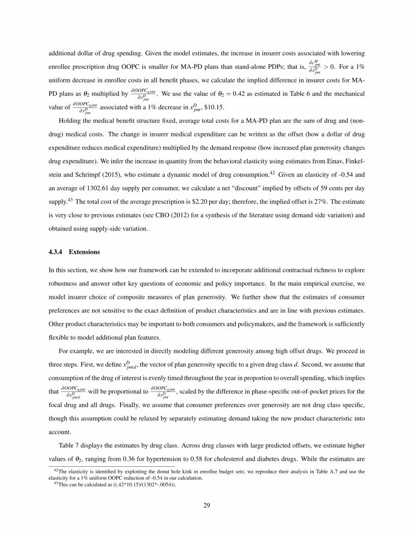
additional dollar of drug spending. Given the model estimates, the increase in insurer costs associated with lowering

enrollee prescription drug OOPC is smaller for MA-PD plans than stand-alone PDPs; that is,∂cM

jmt∂xD

jmt> 0. For a 1%

uniform decrease in enrollee costs in all benefit phases, we calculate the implied difference in insurer costs for MA-

PD plans as θ2 multiplied by ∂OOPCq jmt∂xD

jmt. We use the value of θ2 = 0.42 as estimated in Table 6 and the mechanical

value of ∂OOPCq jmt∂xD

jmtassociated with a 1% decrease in xD

jmt , $10.15.

Holding the medical benefit structure fixed, average total costs for a MA-PD plan are the sum of drug and (non-

drug) medical costs. The change in insurer medical expenditure can be written as the offset (how a dollar of drug

expenditure reduces medical expenditure) multiplied by the demand response (how increased plan generosity changes

drug expenditure). We infer the increase in quantity from the behavioral elasticity using estimates from Einav, Finkel-

stein and Schrimpf (2015), who estimate a dynamic model of drug consumption.42 Given an elasticity of -0.54 and

an average of 1302.61 day supply per consumer, we calculate a net “discount” implied by offsets of 59 cents per day

supply.43 The total cost of the average prescription is $2.20 per day; therefore, the implied offset is 27%. The estimate

is very close to previous estimates (see CBO (2012) for a synthesis of the literature using demand side variation) and

obtained using supply-side variation.

4.3.4 Extensions

In this section, we show how our framework can be extended to incorporate additional contractual richness to explore

robustness and answer other key questions of economic and policy importance. In the main empirical exercise, we

model insurer choice of composite measures of plan generosity. We further show that the estimates of consumer

preferences are not sensitive to the exact definition of product characteristics and are in line with previous estimates.

Other product characteristics may be important to both consumers and policymakers, and the framework is sufficiently

flexible to model additional plan features.

For example, we are interested in directly modeling different generosity among high offset drugs. We proceed in

three steps. First, we define xDjmtd , the vector of plan generosity specific to a given drug class d. Second, we assume that

consumption of the drug of interest is evenly timed throughout the year in proportion to overall spending, which implies

that ∂OOPCq jmt∂xD

jmtdwill be proportional to ∂OOPCq jmt

∂xDjmt

, scaled by the difference in phase-specific out-of-pocket prices for the

focal drug and all drugs. Finally, we assume that consumer preferences over generosity are not drug class specific,

though this assumption could be relaxed by separately estimating demand taking the new product characteristic into

account.

Table 7 displays the estimates by drug class. Across drug classes with large predicted offsets, we estimate higher

values of θ2, ranging from 0.36 for hypertension to 0.58 for cholesterol and diabetes drugs. While the estimates are

42The elasticity is identified by exploiting the donut hole kink in enrollee budget sets; we reproduce their analysis in Table A.7 and use theelasticity for a 1% uniform OOPC reduction of -0.54 in our calculation.

43This can be calculated as ((.42*10.15)/(1302*-.0054)).

29

Table 7: Supply Results, by ClassAsthma Hypertension Diabetes Cholesterol

θ1 -1.170 -1.310 -1.337 -1.343(0.013) (0.014) (0.013) (0.013)

θ2 0.444 0.361 0.576 0.576(0.078) (0.055) (0.059) (0.051)

Plan-Market-Year Obs. 33,538 33,538 33,538 33,538

Notes: Parameters are estimated using generalized method of moments as described in Section 4. Standarderrors are calculated using a bootstrap that re-samples plans with replacement and presented in parentheses.

somewhat noisy, the estimates for asthma, cholesterol, and diabetes are all larger in magnitude than the main estimate

of 0.39, indicating that heterogeneity across drug classes is important in our setting. The estimates are also closely

linked to the reduced form estimates in Figure 2, highlighting the variation in the data that allows us to estimate the

key parameters of interest.

Using our model, we also explore how asymmetric information affects the interpretation of cost side parameters.

First, consistent with the literature, we find evidence of selection with respect to donut hole coverage in Table A.14.

This type of selection may drive our cost parameter estimates. To explore the magnitude of this effect, we estimate the

cost parameters without using variation from the donut hole (i.e., xDjmt = xICR

jmt ), which eliminates selection with respect

to donut hole coverage. Table A.17 presents these cost parameter estimates. Not surprisingly, the parameter estimates

imply less asymmetric information.44 Second, screening incentives could vary by plan type. Lavetti and Simon (2018)

and Lavetti and Han (2017) note that enrollees taking certain drugs are more profitable in MA-PD plans than PDPs.

In contrast to the drug classes in Table 7, the drugs identified in these studies are typically low-volume (e.g., fentanyl).

Table A.17 shows that the results are robust to the exclusion of these drugs: θ2 is not statistically different from our

preferred estimates.

5 Counterfactuals

In this section, we answer two questions with our model and parameter estimates. First, how would stand-alone PDPs

design drug plans if they took externalities into account? Second, how large is the effect relative to distortions due to

asymmetric information? In the counterfactuals, we perturb the key supply-side parameters – θ1 and θ2 – but leave

all other parameters and features of the model fixed. While θ1 and θ2 are equilibrium objects, they have natural

interpretations in specific scenarios. In the absence of offsets and asymmetric information, θ1 =−1 and θ2 = 0.45

44The estimate of θ2 is also slightly attenuated, consistent with smaller differences in cost sharing across plan type in the ICR.45For tractability and clarity, we follow existing studies, including Einav et al. (2013), and do not explicitly model the underlying primitives that

give rise to moral hazard. (They state on page 186, “Our model is designed for conceptual clarity and analytical tractability, both of which come atthe cost of not explicitly modeling the underlying primitives that give rise to ω ,” where ω is the parameter that governs moral hazard.) To interpretthe counterfactuals and for the counterfactual equilibria we calculate to be consistent with the specified game, we need to assume that changes toθ1 and θ2 do not affect plan choice conditional on observables. This assumption encompasses three behavioral restrictions. First, risk adjustmentalgorithms do not directly affect consumer choice. Second, there cannot be selection on moral hazard. Finally (and relatedly), consumers cannot

30

5.1 The Effect of Internalizing Externalities

To quantify the importance of prescription drug offsets, we first consider how stand-alone PDPs would adjust plan

benefit design if they were forced to account for non-drug medical costs in the same way as their counterparts in the

Medicare Advantage program. Given the specification of the supply-side parameters, we can write θPDP = θ1 and

θMA = θ1 + θ2. Mechanically, we set θPDP = θMA and then resolve for a new Nash equilibrium by resolving the

system of first-order conditions described in equation (9). In the counterfactual equilibrium, we allow drug costs to

the insurer, cDjmt , and premiums to adjust to account for the new incentives.46 In the baseline scenario, the average

MA-PD plan has lower premiums (because of generous subsidies) than the average stand-alone PDP, which has an

average premium of $407 per year. By contrast, the average MA-PD plan spends almost $75 dollars more per year on

drugs ($1285 versus $1211).

Table 8 first reports the results of a simulation in which premiums are not allowed to adjust, but stand-alone

PDPs internalize the offset. In the counterfactual, we see that the average stand-alone PDP would spend 7% more on

prescription drugs if they took the entire medical offset into account. In addition, we note that MA-PD plans increase

drug spending: plan generosity is a strategic complement, and there is no implicit trade-off between higher generosity

and higher premiums.

Next we report the results of a counterfactual exercise in which insurers are allowed to adjust both drug spending

and premiums. In contrast to estimation of the empirical model, we now impose optimal bidding. Specifically, in

addition to the previous counterfactual, we require that the first-order conditions with respect to plan bids be satisfied:

pDjmt =

15 ∑

q(cD

q jmt + zDt − sq jmt

∂ sq jmt

∂bDjmt

−1

). (14)

In this simulation, stand-alone PDPs increase drug spending by roughly the same amount, but also increase their

premiums by 10% given the additional drug costs.

The counterfactual benefit design choices have important implications for both enrollees and government budgets.

Critically, the increase in spending on prescription drugs leads to a fiscal savings for the Medicare program through

lower medical expenditures. Our counterfactuals show that stand-alone PDPs would spend $80 more per year if they

took medical expenditure into account, implying an offset of $21.60 per enrollee per year ($22.88 in the counterfactual

that allows for premium adjustment). Multiplying $21.60 by 17.5 million, the number of stand-alone PDP enrollees

in 2008, we find that stand-alone PDPs impose an externality of $378 million per year; based on our bootstrapped

differentially demand insurance contracts that internalize offsets.46We solve for drug costs, rather than benefit design, for three reasons. First, drug costs enter into the insurer’s first-order condition directly.

Second, from a policy perspective, we are primarily interested in impact of different incentives on drug spending. Mechanically, costs change to fitthe model in which the elasticity is taken as given and consumption increases as the cost-sharing schedule changes. Finally, given the monotonicrelationship between the insurer’s choice variables and both OOPC and drug spending, it suffices to solve for the equilibrium outcome. The firstpanel of Table 8 presents the baseline results.

31

estimates, the confidence interval for our estimate ranges from $325 million per year to $431 million per year. By

contrast, McWilliams et al. (2016) find that the much-discussed Medicare Shared Savings Program led to an aggre-

gate $238 million spending reduction in the early years; our larger results indicate the potential power of incentive

alignment in equilibrium. To give additional context, the changes in Medicare Advantage over-payments due to risk

adjustment policies measured in Brown et al. (2014) are approximately $317, or about twice as large as the increase

in drug spending.47

We also calculate a measure of consumer spending that includes OOPC and premiums. In the counterfactual in

which insurers cannot adjust their premiums, consumers benefit from lower OOPC; the effect is slightly larger than

the fiscal savings to the Medicare program. When plans are allowed to adjust their premiums, the effect is partially

offset.48 In both simulations, both consumers and the federal government benefit when PDPs take externalities into

account; in part, this is a transfer from insurers.

5.2 The Relative Importance of Strategic Incentives and Asymmetric Information

We find that strategic incentives created by offsets drive benefit design in the prescription drug insurance market. Yet

a long literature, dating back to the theoretical contributions of Rothschild and Stiglitz (1976), argues that adverse

selection should have a significant impact on benefit design. To better understand the magnitude of strategic incentives

and asymmetric information, we estimate a counterfactual in which we set θ1 = −1 in addition to internalizing the

externality as in the previous counterfactual. Absent asymmetric information or offsets, we expect a one-for-one rela-

tionship between insurer expenditure and enrollee costs. In the counterfactual, all plans face incentives to internalize

offsets, but we have simultaneously eliminated asymmetric information.

Both types of plans become more generous in this counterfactual. In particular, MA-PD plans would become more

generous absent asymmetric information. The magnitude of the effect is the same order of magnitude as the effect of

strategic incentives in the previous counterfactual, though the effects are smaller if premiums are allowed to adjust.

47We would obtain a similar estimate if we used the implied additional spending by stand-alone PDPs in Table 8. By contrast, MedPAC (Medpac(2015)) estimates that spending on an equivalent enrollee in a MA-PD plan is approximately 2% higher than traditional Medicare. The average totalMedicare spending was approximately $10,000 per enrollee in 2008 ($200 of additional spending in MA); the externality due to offsets does not, onits own, imply greater efficiency in MA-PD plans. However, the externality provides evidence of a potential channel through which MA-PD planscan obtain efficiency gains.

Furthermore, Table A.7 shows that it would be costly for the government to achieve the increased drug consumption generated by MA-PD plansusing a flat cost-sharing subsidy alone; this calculation highlights the advantage of nimbler private insurers. However, there is no reason that theprofit maximization incentives of MA-PD plans necessarily align with any social welfare criterion. Therefore, another natural policy interventionwould be to better align consumer plan choices with value (from a societal perspective, including any externalities on the traditional Medicareprogram). Mechanically, we implement this by setting the coefficient on OOPC in the demand system equal to the coefficient on premiums, suchthat consumers treat a $1 increase in premiums equal to a $1 increase in OOPC. The results are in the final two columns of the top panel of TableA.9. If consumers were more "sophisticated" about the potential for underutilization, plans would increase their generosity. MA-PD plans wouldspend 5.6% more on prescription drugs, while stand-alone PDPs would spend 10.4% more. This increased spending by stand-alone PDPs is lessthan the amount that fully internalizes the fiscal externality, yet shows that public policies that align consumer demand or the structure of subsidieswith providing value will lead insurers to offer contracts that reduce costs or increase health.

48We can also calculate a measure that allows consumption to adjust or, alternatively, a measure of consumer surplus (CS) that assumes theparameters of the plan utility function we estimate represent primitive preferences. Given that consumers dislike premium increases more than theylike more generous plans, enrollees are made slightly worse off when premiums are allowed to adjust in the first counterfactual.

32

Table 8: CounterfactualsBaseline

MA PDPPremium 206.00 407.93Insurer Rx Spend 1285.25 1211.62

Counterfactual Plan Counterfactual PlanCharacteristics CharacteristicsMA PDP MA PDP

Internalize Externality: θPDP = θMA = θ1 +θ2Premium 206.21 406.58 214.02 439.41% Change - - 2% 10%Insurer Drug Spend 1332.91 1298.72 1253.89 1295.56% Change 4% 7% -2% 7%Change in Consumer Cost ($/Enrollee) -49.43 -187.04 -41.24 -154.22Fiscal Savings ($/Enrollee) 21.60 22.88Premium Adjustment no yes

No Asymmetric Information, Internalize Externality: θPDP = θMA =−1+θ2Premium 206.21 406.58 159.48 392.43% Change - - 14% 8%Insurer Drug Spend 1373.46 1369.69 1299.33 1390.95% Change 7% 13% 1% 15%Change in Consumer Costs ($/Enrollee) -81.79 -158.01 -136.31 -125.19Fiscal Savings ($/Enrollee) 37.62 44.32Premium Adjustment no yes

Notes: Results are calculated as described in Section 5. Means across markets are reported, as well as the %change from baseline.

33

Stand-alone PDPs also become more generous: stand-alone PDPs would be 7% more generous if they faced the same

strategic incentives as MA-PD plans; they would be 13% more generous if they faced the same strategic incentives

as MA-PD plans and no asymmetric information. The magnitudes are similar if premiums are allowed to adjust.

Given the counterfactual estimates, we conclude that strategic incentives due to benefit integration are as important as

asymmetric information in driving market outcomes.49

In Appendix C, we perform two sets of additional counterfactuals. First, we explore the impact of policy changes

on equilibrium outcomes. Second, we explore the extent to which other features of the economic context – including

behavioral biases and imperfect competition – drive benefit design.

6 Conclusion

This paper examines how health insurers set premiums and design benefits in equilibrium. We build on empirical

literatures that estimate structural models of insurer decisions and model endogenous product characteristics to show

how cost-side incentives affect insurance benefit design. We examine these issues in the Medicare Advantage and Part

D markets and show that differences in incentives across plan types drive the generosity of the plan.

MA-PD plans offer more generous prescription drug plans than their stand-alone counterparts; this increased

generosity is concentrated in those drug categories with large offsets. Our model of firm behavior highlights the

mechanisms that drive this differential: MA-PD plans have an incentive to internalize the effect of medical care

offsets. By measuring firm incentives, we are able to calculate the size of the implied offset. Our estimate of an

approximately 27% offset is similar in magnitude to demand-side estimates in the literature (Chandra, Gruber and

McKnight (2010); Gaynor, Li and Vogt (2007)). The counterfactuals show how policy changes can increase plan

incentives to help enrollees internalize offsets and explore the impact of alternative subsidies.

Government policy plays an important and understudied role in determining how market forces will affect health

care utilization and consumer welfare in the Medicare program. Our framework can be used to further explore en-

dogenous product design in selection markets and can help researchers model firm behavior and measure welfare in an

“endogenous contracts framework” (Geruso and Layton (2018)). Thus, we build on an existing literature that considers

premium setting conditional on fixed plan characteristics (Handel (2013); Lustig (2010); Starc (2015); Town and Liu

(2003); Tebaldi (2017); Ericson and Starc (2015)). Future work should explore the impact of supply-side regulation,

including premium and contract regulation, within the context of a rich model that does not require fixed insurance

contracts.

49This finding is consistent with Starc (2015), which finds that strategic firm incentives, rather than adverse selection, drive firm behavior (in thatinstance, premiums) and margins in a similar setting.

34

References

Abaluck, Jason and Jonathan Gruber. 2011. “Choice Inconsistencies among the Elderly: Evidence from Plan Choice

in the Medicare Part D Program.” American Economic Review 101(4):1180–1210.

Abaluck, Jason and Jonathan Gruber. 2016. “Evolving Choice Inconsistencies in Choice of Prescription Drug Insur-

ance.” American Economic Review 106(8):2145–84.

Abaluck, Jason, Jonathan Gruber and Ashley Swanson. 2018. “Prescription Drug Use under Medicare Part D: A

Linear Model of Nonlinear Budget Sets.” Journal of Public Economics 164:106–138.

Afendulis, Christopher C, Michael E Chernew and Daniel P Kessler. 2017. “The Effect of Medicare Advantage on

Hospital Admissions and Mortality.” American Journal of Health Economics 3(2):254–279.

Afendulis, Christopher C., Yulei He, Alan M. Zaslavsky and Michael E. Chernew. 2011. “The Impact of Medicare

Part D on Hospitalization Rates.” Health Services Research 46(4):1022–1038.

Baicker, Katherine and Dana Goldman. 2011. “Patient Cost-sharing and Healthcare Spending Growth.” Journal of

Economic Perspectives 25(2):47–68.

Baicker, Katherine, Michael E. Chernew and Jacob Robbins. 2013. “The Spillover Effect of Medicare Managed Care:

Medicare Advantage and Hospital Utilization.” Journal of Health Economics 32:1289–1300.

Baicker, Katherine, Sendhil Mullainathan and Joshua Schwartzstein. 2015. “Behavioral Hazard in Health Insurance.”

Quarterly Journal of Economics 130(4):1623–1667.

Berry, Steven. 1994. “Estimating Discrete Choice Models of Product Differentiation.” RAND Journal of Economics

25:242–262.

Berry, Steven and Panle Jia. 2010. “Tracing the Woes, an Empirical Analysis of the Airline Industry.” American

Economic Journal: Microeconomics 2(3):1–43.

Brot-Goldberg, Zarek C, Amitabh Chandra, Benjamin R Handel and Jonathan T Kolstad. 2017. “Consumer Het-

erogeneity and Medical Care Price Responsiveness: Evidence and Implications for Optimal Insurance Design.”

Quarterly Journal of Economics 132(3):1261–1318.

Brown, J., M. Duggan, I. Kuziemko and W. Woolston. 2014. “How Does Risk-Selection Respond to Risk-Adjustment:

Evidence from the Medicare Advantage Program.” American Economic Review 104(10):3335–64.

Cabral, Marika, Michael Geruso and Neale Mahoney. 2018. “Do Larger Health Insurance Subsidies Benefit Patients

or Producers? Evidence from Medicare Advantage.” American Economic Review 108(8):2048–2087.

35

Cabral, Marika and Neale Mahoney. 2019. “Externalities and Taxation of Supplemental Insurance: A Study of Medi-

care and Medigap.” American Economic Journal: Applied Economics 11(2):37–73.

Carey, C.M. 2017. “Technological Change and Risk Adjustment: Benefit Design Incentives in Medicare Part D.”

American Economic Journal: Economic Policy 9(1):38–73. Cornell University.

CBO. 2012. Offsetting Effects of Prescription Drug Use on Medicares Spending for Other Health Care Services.

Technical report Congressional Budget Office.

Chandra, Amitabh, Jonathan Gruber and Robin McKnight. 2010. “Patient cost-sharing and hospitalization offsets in

the elderly.” American Economic Review 100(1).

Chernew, Michael E, Allison B Rosen and A Mark Fendrick. 2007. “Value-based insurance design.” Health Affairs

26(2):w195–w203.

Crawford, G. 2012. “Accommodating Endogenous Product Choices: A Progress Report.” International Journal of

Industrial Organization 30:315–320.

Curto, Vilsa, Liran Einav, Jonathan Levin and Jay Bhattacharya. 2015. “Can Health Insurance Competition Work?

Evidence from Medicare Advantage.” NBER Working Paper No. 20818.

Dalton, Christina M., Gautam Gowrisankaran and Robert Town. 2015. “Myopia and Complex Dynamic Incentives:

Evidence from Medicare Part D.” NBER Working Paper No. 21104.

Decarolis, F. 2015. “Medicare Part D: Are Insurers Gaming the Low Income Subsidy Design?” American Economic

Review 105(4):1547–80.

Decarolis, Francesco, Maria Polyakova and Steven P. Ryan. Forthcoming. “Subsidy Design in Privately-Provided

Social Insurance: Lessons from Medicare Part D.” Journal of Political Economy .

Draganska, M., M. Mazzeo and K. Seim. 2009. “Beyond Plain Vanilla: Modeling Joint Product Assortment and

Pricing Decisions.” Quantative Marketing and Economics 7(2).

Duggan, Mark, Amanda Starc and Boris Vabson. 2016. “Who Benefits when Government Pays more? Pass-through

in the Medicare Advantage Program.” Journal of Public Economics 141:50–67.

Einav, L., A. Finkelstein, S. Ryan, P. Schrimpf and M. Cullen. 2013. “Selection on Moral Hazard in Health Insurance.”

American Economic Review 103(1):178–219.

Einav, Liran, Amy Finkelstein and Maria Polyakova. 2016. “Private Provision of Social Insurance: Drug-specific Price

Elasticities and Cost Sharing in Medicare Part D.” American Economic Journal: Economic Policy 10(3):122–153.

36

Einav, Liran, Amy Finkelstein and Paul Schrimpf. 2015. “The Response of Drug Expenditures to Non-linear Contract

Design: Evidence from Medicare Part D.” Quarterly Journal of Economics 130(2):841–899.

Eizenberg, A. 2014. “Upstream Innovation and Product Variety in the U.S. Home PC Market.” Review of Economic

Studies 81:1003–1045.

Ellis, Randall P., Shenyi Jiang and W. Manning. 2015. “Optimal Health Insurance for Multiple Goods and Time

Periods.” Journal of Health Economics 41:89–106.

Ericson, K. 2014. “Consumer Inertia and Firm Pricing in the Medicare Part D Prescription Drug Insurance Exchange.”

American Economic Journal: Economic Policy 6(1):38–64.

Ericson, Keith and Amanda Starc. 2015. “Pricing Regulation and Imperfect Competition on the Massachusetts Health

Insurance Exchange ,.” Review of Economics and Statistics 97(3):667–682.

Ericson, Keith and Amanda Starc. 2016. “How Product Standardization Affects Choice: Evidence from the Mas-

sachusetts Health Insurance Exchange.” Journal of Health Economics 50:71–85.

Fan, Y. 2013. “Ownership Consolidation and Product Characteristics: A Study of the US Daily Newspaper Market.”

American Economic Review 103(5):1598–1628.

Finkelstein, Amy, Matthew Gentzkow and Heidi Williams. 2016. “Sources of Geographic Variation in Health Care:

Evidence from Patient Migration.” Quarterly Journal of Economics 131(4):1681–1726.

Gaynor, M., J. Li and W. Vogt. 2007. “Substitution, Spending Offsets, and Prescription Drug Benefit Design.” Forum

for Health Economics and Policy 10(2):1–31.

Geruso, M. and T. J. Layton. 2018. “Selection in Health Insurance Markets and Its Policy Remedies.” Journal of

Economic Perspectives 31(4):23–50.

Geruso, Michael, Timothy J. Layton and Daniel Prinz. Forthcoming. “Screening in Contract Design: Evidence from

the ACA Health Insurance Exchanges.” American Economic Journal: Economic Policy 11(2):64–107.

Glazer, J. and T. McGuire. 2013. “A Welfare Measure of Offset Effects in Health Insurance.” Journal of Public

Economics 96(5-6):520–523.

Goldman, D. and Tomas J. Philipson. 2007. “Integrated Insurance Design in the Presence of Multiple Medical Tech-

nologies.” American Economic Review 97(2):427–432.

Goldman, Dana P, Geoffrey F Joyce and Yuhui Zheng. 2007. “Prescription Drug Cost Sharing: Associations with Med-

ication and Medical Utilization and Spending and Health.” Journal of the American Medical Association 298(1):61–

69.

37

Gowrisankaran, G., K. Norberg, S. Kymes, M. E. Chernew, D. Stwalley, L. Kemper and W. Peck. 2013. “A Hospital

System’s Wellness Program Linked To Health Plan Enrollment Cut Hospitalizations But Not Overall Costs.” Health

Affairs 32(3):477–485.

Handel, B. R. and J. T. Kolstad. 2015. “Getting the Most From Marketplaces: Smart Policies on Health Insurance

Choice.” Brookings Hamilton Project Discussion Paper 2015-08.

Handel, Benjamin. 2013. “Adverse Selection and Inertia in Health Insurance Markets: When Nudging Hurts.” Ameri-

can Economic Review (103):2643–2682.

Heiss, F., D. McFadden, J. Winter, A. Wupperman and B. Zhou. 2016. “Inattention and Switching Costs as Sources of

Inertia in Medicare Part D.” NBER Working Paper No. 22765.

Ho, K., J. Hogan and F. Scott Morton. 2015. “The Impact of Consumer Inattention on Insurer Pricing in the Medicare

Part D Program.” NBER Working Paper No. 21028.

Hoadley, J., L. Summer, E. Hargrave, J. Cubanski and T. Neuman. 2014. “Medicare Part D in Its Ninth Year: The

2014 Marketplace and Key Trends, 2006-2014.”.

Hortascu, A., S.A. Madanizadeh and S. Puller. 2015. “Power to Choose? An Analysis of Consumer Inertia in the

Residential Electricity Market.” NBER Working Paper No. 20988.

Hsu, J., J. Huang, V. Fung, M. Price, R. Brand, R. Hui, B. Fireman, W. Dow, J. Bertko and J. Newhouse. 2009.

“Distributing 800 Billion: An Early Assessment Of Medicare Part D Risk Adjustment.” Health Affairs 28(1):215–

225.

Ketcham, J., C. Lucarelli, E. Miravete and M. Roebuck. 2012. “Sinking, Swimming, or Learning to Swim in Medicare

Part D.” American Economic Review 102(6):2639–2673.

Lavetti, K. and T. Han. 2017. “Does Part D Abet Advantageous Selection in Medicare Advantage?” Journal of Health

Economics 56:368–382.

Lavetti, Kurt and Kosali Simon. 2018. “Strategic Formulary Design in Stand-Alone and Integrated Medicare Advan-

tage Prescription Drug Plans.” American Economic Journal: Economic Policy 10(3):154–192.

Lustig, J. 2010. “Measuring welfare losses from adverse selection and imperfect competition in privatized medicare.”

Boston University Department of Economics.

Maciejewski, Matthew L, Chris L Bryson, Mark Perkins, David K Blough, Francesca E Cunningham, John C Fortney,

Sarah L Krein, Kevin T Stroupe, Nancy D Sharp and Chuan Fen Liu. 2010. “Increasing Copayments and Adherence

38

to Diabetes, Hypertension, and Hyperlipidemic Medications.” The American Journal of Managed Care 16(1):e20–

34.

Maciejewski, Matthew L, Joel F Farley, John Parker and Daryl Wansink. 2010. “Copayment reductions generate

greater medication adherence in targeted patients.” Health affairs 29(11):2002–2008.

Manning, W., J. Newhouse, N. Duan, E. Keeler, B. Benjamin, A. Leibowitz and M. Marquis. 1987. “Health Insur-

ance and the Demand for Medical Care: Evidence from a Randomized Experiment.” American Economic Review

77(3):251–277.

McGuire, T., J. Newhouse and A. Sinaiko. 2011. “An Economic History of Medicare Part C.” Milbank Quarterly

89(2):289–332.

McGuire, Thomas G. 2011. Demand for health insurance. In Handbook of health economics. Vol. 2 Elsevier pp. 317–

396.

McWilliams, J. Michael, Alan M. Zaslavsky and Haiden A. Huskamp. 2011. “Implementation of Medicare Part D and

Nondrug Medical Spending for Elderly Adults With Limited Prior Drug Coverage.” The Journal of the American

Medical Association 306(4):402–409.

McWilliams, J.M., L. Hatfield, M.E. Chernew, B. Landon and A. Schwartz. 2016. “Early Performance of Accountable

Care Organizations in Medicare.” New England Journal of Medicine 374:2357–2366.

Medpac. 2015. “The Medicare Advantage program: Status report.”.

Medpac. 2016. Report to the Congress: Medicare and the Health Care Delivery System. Technical report Medpac.

Miller, D. and J. Yeo. 2014. “A Dynamic Discrete Choice Model of Switching Costs in Medicare Part D.” Clemson

University and Singapore Management University Unpublished Mimeo.

Newhouse, J., M. Price, J. McWilliams, J. Hsu and T. McGuire. 2015. “How Much Favorable Selection is Left in

Medicare Advantage?” American Journal of Health Economics 1(1):1–26.

NICE. 2011. Hypertension in adults: diagnosis and management. Technical report National Institute for Health and

Care Excellence.

Nosal, K. 2011. “Estimating Switching Costs for Medicare Advantage Plans.” Mannheim.

Polyakova, M. 2016. “Regulation of Insurance with Adverse Selection and Switching Costs: Evidence from Medicare

Part D.” American Economic Journal: Applied Economics 8(3):165–195.

39

Rothschild, Michael and Joseph Stiglitz. 1976. “Equilibrium in Competitive Insurance Markets: An Essay on the

Economics of Imperfect Information.” Quarterly Journal of Economics pp. 629–649.

Starc, A. 2015. “Insurer Pricing and Consumer Welfare: Evidence From Medigap.” RAND Journal of Economics

45(1):198–220.

Sweeting, A. 2010. “The Effects of Mergers on Product Positioning: Evidence from the Music Radio Industry.” RAND

Journal of Economics 41(2):372–97.

Tebaldi, P. 2017. “Estimating Equilibrium in Health Insurance Exchanges: Price Competition and Subsidy Design

under the ACA.” 2017.

Town, R. and S. Liu. 2003. “The Welfare Impact of Medicare HMOs.” RAND Journal of Economics 32(4):719–736.

Train, K. 2009. Discrete Choice Methods with Simulation. Cambridge University Press.

Wollman, T. 2018. “Trucks without bailouts: Equilibrium product characteristics for commercial vehicles.” American

Economic Review 108(6):1364–1406.

Wu, Y. 2016. “Supply Response to Consumer Inertia: Strategic Pricing in Medicare Part D.” MIT Unpublished Memo.

40

Appendices

A Utilization and Insurer Spending

A.1 Reduced Form Relationship Between Benefit Design and Insurer Costs

We regress insurer costs on our key product characteristics: x jmt =

[xICR

jmt , xDonutjmt

]′. The results are in Table A.1. In

all specifications, we control for contract fixed effects, and risk quintile to capture underlying contract characteristics

and consumer risk.50 In our second and third specifications, we also control for demographic characteristics (age, race,

and gender), which capture part of the observable risk. In our final, most conservative specifications, we also control

for historical county-level FFS spending, which proxies for county level variation in medical services, including drugs,

that might be driven by differences in patient preferences, medical care infrastructure, and the physician culture (see

Finkelstein, Gentzkow and Williams (2016)).

Table A.1: Benefit Design and Insurer CostsDependent Variable: Insurer Costs

(1) (2) (3) (4) (5) (6)xICR

jmt -672.9*** -673.4*** -672.4*** -674.2*** -673.6*** -675.6***(95.23) (139.9) (94.65) (140.9) (94.93) (140.4)

xDonutjmt -25.39 -66.38** -25.60 -65.09** -25.09 -65.62**

(18.02) (30.78) (18.02) (30.55) (17.94) (30.47)1(MA)∗ xICR

jmt -1.014 -0.279 1.241(158.0) (158.6) (158.2)

1(MA)∗ xDonutjmt 54.86* 53.40 54.48*

(32.68) (32.49) (32.47)FFS Costs 0.388*** 0.388***

(0.0375) (0.0374)R-Squared 0.243 0.245 0.245 0.243 0.246 0.246Observations 569,078 569,078 569,078 569,078 569,078 569,078Year FE X X X X X XRisk Quintile FE X X X X X XDemo. Controls X X X XPlan FE X X X X X X

Notes: Table presents OLS regression models, where outcome variable is insurer costs. The unit ofobservation is an enrollee-year for the 2007-2009 period. The original data are obtained from a 10% sampleof CMS prescription drug event files, aggregated to the enrollee-year level. We include year-level indicatorsand indicators for the quintile of 2006 spending (consumer types) in all specifications. In somespecifications, we also control for 5-yr average per capita Medicare FFS spending and demographic controlsfor age categories, race, and gender. Standard errors are clustered at the contract level and are presented inparentheses. Statistical significance at the 10%, 5%, and 1% levels are denoted by *, **, and ***respectively.

The results show that higher costs for enrollees are associated with lower insurer drug costs: a $1 increase in

enrollee cost per day supply in the ICR is associated with $675 less in insurer drug spending. The effect for the donut50Therefore, we are leveraging within contract variation across geographic space and over time.

41

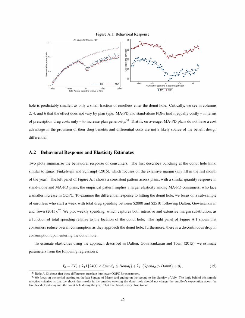
Figure A.1: Behavioral Response

.7.8

.91

Shar

e w

ith D

ecem

ber C

laim

-2000 -1000 0 1000 2000Total Annual Spending relative to Kink

MA PDP

All Drugs for MA vs. PDP

7075

8085

90M

ean

spen

ding

per

wee

k

-400 -200 0 200 400Cumulative spending at beginning of week

MA PDP

hole is predictably smaller, as only a small fraction of enrollees enter the donut hole. Critically, we see in columns

2, 4, and 6 that the effect does not vary by plan type: MA-PD and stand-alone PDPs find it equally costly – in terms

of prescription drug costs only – to increase plan generosity.51 That is, on average, MA-PD plans do not have a cost

advantage in the provision of their drug benefits and differential costs are not a likely source of the benefit design

differential.

A.2 Behavioral Response and Elasticity Estimates

Two plots summarize the behavioral response of consumers. The first describes bunching at the donut hole kink,

similar to Einav, Finkelstein and Schrimpf (2015), which focuses on the extensive margin (any fill in the last month

of the year). The left panel of Figure A.1 shows a consistent pattern across plans, with a similar quantity response in

stand-alone and MA-PD plans; the empirical pattern implies a larger elasticity among MA-PD consumers, who face

a smaller increase in OOPC. To examine the differential response to hitting the donut hole, we focus on a sub-sample

of enrollees who start a week with total drug spending between $2000 and $2510 following Dalton, Gowrisankaran

and Town (2015).52 We plot weekly spending, which captures both intensive and extensive margin substitution, as

a function of total spending relative to the location of the donut hole. The right panel of Figure A.1 shows that

consumers reduce overall consumption as they approach the donut hole; furthermore, there is a discontinuous drop in

consumption upon entering the donut hole.

To estimate elasticities using the approach described in Dalton, Gowrisankaran and Town (2015), we estimate

parameters from the following regression i:

Yit = FEi +λ11{2400 < Spendit ≤ Donutt}+λs1{Spendit > Donut}+υit , (15)

51Table A.13 shows that these differences translate into lower OOPC for consumers.52We focus on the period starting on the last Sunday of March and ending on the second to last Sunday of July. The logic behind this sample

selection criterion is that the shock that results in the enrollee entering the donut hole should not change the enrollee’s expectation about thelikelihood of entering into the donut hole during the year. That likelihood is very close to one.

42

Table A.2: Behavioral Response(1) (2) (3)

ln(1 + Spending) ln(1 + day supply) ln(1 + Enrollee Cost)At Kink -0.0564*** -0.0439*** 0.114***

(0.00377) (0.00331) (0.000999)At Kink * MA -0.00761 0.000704 -0.0123***

(0.00770) (0.00691) (0.00227)Post Kink -0.103*** -0.0804*** 0.151***

(0.00217) (0.00190) (0.000684)Post Kink * MA -0.0364*** -0.0227*** -0.0208***

(0.00459) (0.00409) (0.00154)N 5,220,060 5,220,060 2,452,070

Notes: Standard errors are in parentheses. All regressions include enrollee fixed effects and cluster standard errors at theenrollee level. Each observation is an enrollee-week for enrollees that have beginning-of-week spending in the interval[Kink - $510, Kink) sometime between week 14 and week 30 of the calendar year and enrollee-weeks withbeginning-of-week spending in the interval [Kink - $510, Kink + $490]. * p<0.05 ** p<0.01 *** p<0.001

where Yit is the weekly drug spending for individual i in week t, FEi is an individual fixed effect, Spendit is the

total drug spending in that year at the beginning of week t for individual i, Donut is the dollar value of the initiation of

the coverage gap phase of the benefit package in that year, and υit is an i.i.d. error term. The individual fixed effects

control for individual selection into the donut hole. Identification is driven by variation in the timing of entering the

donut hole controlling for mean individual characteristics. Given our sample selection, λs coefficient measures the

mean impact of transitioning into the donut hole phase. We estimate this equation separately for PDP and MA-PD

enrollees.

The parameter estimates are presented in Table A.2. Consistent with the reduced form analysis, enrollee costs

increase as consumers enter the donut hole: the average enrollee cost increases by 15% for consumers in stand-alone

PDPs and 13% for consumers in MA-PD plans. Consistent with the results presented in Figure A.1, the parameter

estimates show that upon entering the donut hole, PDP enrollees drop their spending an average of 10%. In contrast,

MA-PD enrollees reduce their spending by 14% upon entering the donut hole; the larger response reflects both a great

extensive margin demand elasticity and a shift to lower cost drugs.53 Comparing these estimates to the estimates of the

differences in OOPC between PDP and MA-PD plans implies a donut hole elasticity ranging from -0.53 (stand-alone

PDPs) to -0.79 (MA-PD plans).54

53There are two points to note here. First, we argue below that MA-PD enrollment leads to a causal increase in average consumption. Second,we find no evidence of an increased drop in consumption upon entering the donut hole among high offset drugs. Exploring heterogeneity in thiseffect is an interesting direction for future work.

54Because the elasticity of demand can be written as the percentage change in day supply divided by the percentage change in price post-kink, wedivide the coefficient on “Post Kink” in column 2 (where logged day supply is the dependent variable) by the coefficient on “Post Kink” in column3.

43

A.3 Total Annual Expenditure

Our goal is to estimate the causal impact of MA-PD enrollment on total drug consumption, insurer, and enrollee

drug costs. However, a naive estimate will be contaminated by selection, as MA-PD enrollees are likely healthier

than stand-alone PDP enrollees. Therefore, on average, MA-PD enrollees will have lower drug expenditure than their

counterparts in stand-alone PDPs for reasons other than benefit design. This is likely to be true even once we control

for a rich set of individual characteristics.

As discussed above, consumers in urban floor counties close to the threshold are more likely to be enrolled in

MA-PD plans than consumers in similar rural floor counties just to the right of the urban threshold.55 In our reduced

form analysis, we use the county urban/rural status as an instrument in a linear instrumental variable specification; the

empirical strategy is a fuzzy regression discontinuity approach.

The variation we use in IV specifications is highlighted in Figure A.2, which plots the probability of MA-PD

enrollment as a function of population. This figure depicts a binscatter plot with twenty population bins. We control

for consumer demographics, including risk quintile, as well as annual mean county-level FFS spending and plot the

average probability of MA-PD enrollment. We fit quadratic curves on either side of the 250,000 population cutoff. We

see a dramatic change in the probability of MA-PD enrollment just to the right of the discontinuity. We implement the

identification strategy using an instrument variables framework. Specifically, we estimate:

yi jmt = X1mtβ1 +X2

it β2 +β31(MA-PD jmt)+g1(popmt)+µi jmt , (16)

1(MA-PD jmt) = X1mtγ1 +X2

it γ2 + γ31(urbanmt)+g2(popmt)+νi jmt, (17)

where β3 is the coefficient of interest, and X1mt and X2

it are vectors of market and individual specific covariates, re-

spectively. In all specifications, we control flexibly for metro area population. The dependent variables of interest,

yit jm, are total drug spending, consumer OOPC, and insured costs, where j represents a plan. We hypothesize that

insured spending is causally higher in MA-PD plans, and enrollee OOPC lower. These relationships are due directly

to benefit design on the part of insurers; the overall impact of these changes on total expenditure is more ambiguous,

as it depends on the size of the behavioral response, but likely to be positive as well.

To explore the impact of Medicare Advantage enrollment on consumption, we focus on the 2007-2009 time period.

In all specifications, we control for the consumer quintile of 2006 drug spending, calculated at the national level. In the

second and third specifications, we also control for demographic characteristics (age, race, and gender), which capture

part of the observable risk. In the final, most conservative specifications, we also control for historical county-level

FFS spending, which proxies for county level variation in medical services, including drugs, that might be driven by

55We will also use urban status to predict the inside share of MA-PD plans in the plan choice models.

44

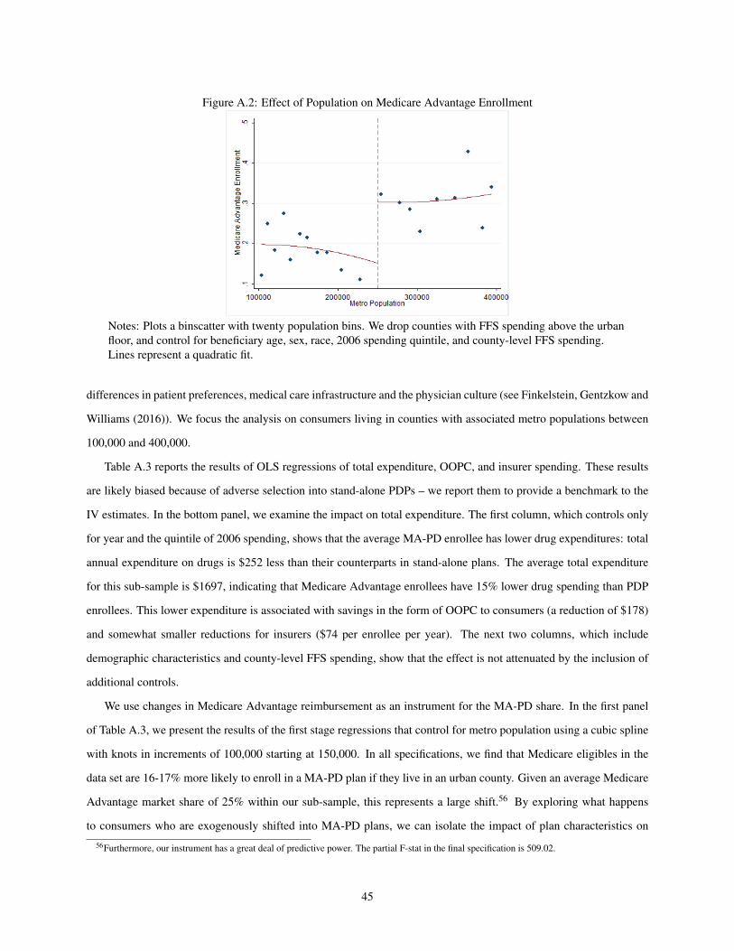
Figure A.2: Effect of Population on Medicare Advantage Enrollment

Notes: Plots a binscatter with twenty population bins. We drop counties with FFS spending above the urbanfloor, and control for beneficiary age, sex, race, 2006 spending quintile, and county-level FFS spending.Lines represent a quadratic fit.

differences in patient preferences, medical care infrastructure and the physician culture (see Finkelstein, Gentzkow and

Williams (2016)). We focus the analysis on consumers living in counties with associated metro populations between

100,000 and 400,000.

Table A.3 reports the results of OLS regressions of total expenditure, OOPC, and insurer spending. These results

are likely biased because of adverse selection into stand-alone PDPs – we report them to provide a benchmark to the

IV estimates. In the bottom panel, we examine the impact on total expenditure. The first column, which controls only

for year and the quintile of 2006 spending, shows that the average MA-PD enrollee has lower drug expenditures: total

annual expenditure on drugs is $252 less than their counterparts in stand-alone plans. The average total expenditure

for this sub-sample is $1697, indicating that Medicare Advantage enrollees have 15% lower drug spending than PDP

enrollees. This lower expenditure is associated with savings in the form of OOPC to consumers (a reduction of $178)

and somewhat smaller reductions for insurers ($74 per enrollee per year). The next two columns, which include

demographic characteristics and county-level FFS spending, show that the effect is not attenuated by the inclusion of

additional controls.

We use changes in Medicare Advantage reimbursement as an instrument for the MA-PD share. In the first panel

of Table A.3, we present the results of the first stage regressions that control for metro population using a cubic spline

with knots in increments of 100,000 starting at 150,000. In all specifications, we find that Medicare eligibles in the

data set are 16-17% more likely to enroll in a MA-PD plan if they live in an urban county. Given an average Medicare

Advantage market share of 25% within our sub-sample, this represents a large shift.56 By exploring what happens

to consumers who are exogenously shifted into MA-PD plans, we can isolate the impact of plan characteristics on

56Furthermore, our instrument has a great deal of predictive power. The partial F-stat in the final specification is 509.02.

45

Table A.3: Impact of MA-PD Enrollment on Drug Spending(1) (2) (3) (4) (5) (6)

OLS IVFirst Stage, Dependent Variable: MA-PD Enrollment1 (Urban) 0.168*** 0.170*** 0.177***

(0.00785) (0.00785) (0.00787)R-squared 0.026 0.036 0.037Dependent Variable: Insurer Drug Expenditure1(MA-PD) -74.21*** -76.25*** -73.32*** 514.2*** 506.7*** 387.5***

(3.969) (3.973) (3.972) (74.25) (73.35) (68.38)FFS 5 Year 0.430*** 0.506***Avg. Spend (0.0189) (0.0226)

R-Squared 0.217 0.219 0.221 0.114 0.119 0.159Dependent Variable: Enrollee Drug Expenditure1(MA-PD) -177.5*** -174.6*** -173.3*** -215.2*** -222.2*** -265.2***

(2.850) (2.861) (2.863) (55.51) (54.92) (52.74)FFS 5 Year 0.198*** 0.183***Avg. Spend (0.0160) (0.0183)

R-Squared 0.193 0.195 0.195 0.193 0.194 0.192Dependent Variable: Total Drug Expenditure1(MA-PD) -251.7*** -250.9*** -246.6*** 299.0*** 284.6*** 122.3

(5.851) (5.870) (5.873) (108.0) (106.7) (100.7)FFS 5 Year 0.628*** 0.688***Avg. Spend (0.0298) (0.0343)

R-Squared 0.264 0.265 0.267 0.230 0.233 0.252Year FE X X X X X XRisk Quintile FE X X X X X XDemo. X X X XControls

N 381921 381921 381921 381921 381921 381921Sample 100-400K 100-400K 100-400K 100-400K 100-400K 100-400K

Notes: Table presents linear regression models, where outcome variables are insurer and enrollee costs andtotal expenditure levels. The unit of observation is at the enrollee-year level, for the 2007-2009 period. Theoriginal data are obtained from a 10% sample of CMS prescription drug event files, aggregated to theenrollee-year level. We restrict to those counties in the 100-400k metro population band. We includeyear-level indicators and indicators for the quintile of 2006 spending in all specifications. In somespecifications, we also control for 5-year average per capita Medicare FFS spending, from 2007. We alsoinclude controls for age, age squared, race, and gender as demographic controls. In addition, we include aspline of metro population. Standard errors are clustered at the product level and are presented inparentheses. Statistical significance at the 10%, 5%, and 1% levels are denoted by *, **, and ***respectively.

46

consumption.

The second panel of Table A.3 shows the estimated impact of MA-PD enrollment on insurer drug costs. Once we

account for differential selection, MA-PD plans spend much more on drugs than stand-alone PDPs. The estimate of

$514 in column 4 is approximately half of average insurer spending across all plans ($1031 per enrollee per year).

This estimate is more attenuated in the final column (albeit not statistically different from the estimates in column

4), which includes historical, county-level FFS costs as an additional control. Here the estimates indicate that MA-

PD plans spend $388 more per year than stand-alone PDPs for an equivalent enrollee. As expected, historical FFS

spending influences drug consumption: Finkelstein, Gentzkow and Williams (2016) find that approximately half of all

variation in spending is due to place-specific supply factors. The following panels describe the impact of additional

insurer spending on consumers. The third panel shows that a consumer enrolled in Medicare Advantage can expect to

spend $265 less per year on drugs, holding health risk constant. Consumer spending does not fall one-for-one with the

increase in insurer spending, implying that the reduction in average OOPC for consumers increases consumption, as

confirmed in the final panel. In our preferred estimates, the causal impact of MA-PD enrollment is somewhat noisy,

but implies a $122 increase in drug consumption. On a base of $1697 of drug spending per year, this represents a 7%

increase in spending. Total drug consumption increases despite a drop in consumer spending.

We hypothesize that the underlying mechanism driving an increase in drug consumption from Medicare Advan-

tage enrollment is differences in MA-PD benefit design intended to internalize the impact of offsets on non-drug

medical spending. In support of this hypothesis, we show that the effect of Medicare Advantage enrollment on drug

consumption is driven entirely by drugs believed to have large offsets a priori. We explore the total enrollee level of

consumption of “Category 1” drugs, as classified by Chandra, Gruber and McKnight (2010). If these drugs are not

taken when prescribed, a serious event, such as a hospitalization, is significantly more likely to occur within the next

six months.57

Table A.4 describes these results. About 40% of average expenditure ($648.11) is concentrated in these “Category

1” drugs. Consistent with previous specifications, the OLS results are biased downward due to advantageous selection

57“Category 1” drugs are “acute care drugs are those that, if not taken, will increase the probability of an adverse health event within a month ortwo.” These drugs comprise approximately 40% of total drug spending. Category 2 contains “chronic care medications are designed to treat morepersistent conditions that, if not treated, will result in a potentially adverse health event within the year (examples include analgesics, antivirals,ACE inhibitors, medications, beta-blockers, hypertension drugs, statins, and glaucoma medications).” Category 3 are “medications that, whilenecessary to improve patients’ quality of life, will not result in an adverse health event if not taken, because they provide symptom relief as opposedto affecting the underlying disease process (examples are acne medications, antihistamines, motion sickness medications, cold remedies, relief ofpain drugs).”

The classes included in “Category 1” are Adrenal Corticosteroids, Aminoglycosides, Anaphylaxis Treatment Kits, Anesthesia, Anthelmintics,Antianginals, Antiarrhythmics, Antiasthmatics and broncodilators, Antibacterials, Miscellaneous, Antibiotics, Alkaloids, And Enzymes, Antico-agulants/thrombolytics, Anticonvulsants, Antidotes, Antimalarials, Antimetabolites, Antimycobacterials, Antineoplastics, Antiprotozoals, Antipsy-chotics/antimanics, Antitoxins/antivenins, Blood Components/substitutes, Blood Glucose Regulators, Cardiac Glycosides, Cardiovascular-renal,Cephalosporins, Chloramphenicol/derivatives, Coronary Vasodilators, Dna Damaging Drugs, Hypotension/shock, Lincosamides and macrolides,Ocular Anti-infective/anti-inflammator, Penicillins, Polymyxins, Quinolones/derivatives, Repl/regs Of Electrolytes/water Balance, RespiratoryTract, Sulfonamides/related Compounds, Tetracyclines, Vascular Disorders, and Cerebral/peripheral. We exclude drugs that are believed to havedifferential selection effects, as described in Lavetti and Simon (2018). Drug lists for each category were compiled using lists from drugs.com. Res-piratory tract drugs include drugs used to treat asthma and COPD. For drugs with multiple uses, the drug was only included under its primary usage(e.g. etanercept is sometimes used to treat Alzheimer’s Disease, but is much more commonly used for autoimmune diseases such as rheumatoidarthritis, psoriatic arthritis, plaque psoriasis and ankylosing spondylitis. Thus, it is not included on the list of Alzheimer’s drugs).

47

into MA-PD plans. However, the IV specifications in columns 3-6 show a consistent pattern: MA-PD enrollees

consume proportionally more of these “Category 1” drugs, due in large part to greater insurer expenditure. MA-PD

enrollment leads to an additional $156 in annual expenditure on these drugs; on a base of $648, this amounts to a 24%

increase, versus 7% for total drug consumption. Put differently, all of the increased total expenditure in MA-PD plans

is concentrated in these large offset drugs. Total expenditure in this category increases by $156, while overall total

expenditure increases by $122, implying that MA-PD plans do not spend more on drugs that are unlikely to have large

offsets.

B Risk Stabilization and Regulation

In this appendix, we describe risk stabilization by CMS and its effect on firm incentives. CMS uses a three-

pillar system to mitigate adverse selection in Part D; as a result, the impact of adverse selection is muted, though not

necessarily eliminated. Most importantly, risk adjustment could affect the relative profitability of different Medicare

beneficiaries. The Part D program also affects insurer costs ex post in two key ways. First, catastrophic reinsurance

mitigates costs for especially sick enrollees. Second, risk corridor transfers limit both upside and downside risk to

insurers.

B.1 Risk Adjustment

Risk adjustment attempts to equalize insurer profitability across beneficiaries by increasing subsidies for sicker

enrollees. Despite this, there may still be selection conditional on the risk adjustment (Brown et al. (2014); Carey

(2017)). We incorporate risk adjustment into the formulation of insurer costs. Drug costs cDi jmt(xD

mt,rit ,ηi jmt) =

cDi jmt(xD

mt,rit)+ηi jmt are not fully compensated by risk-adjustment and are a function of the entire vector of prod-

uct characteristics, xDmt, the individual’s risk score, rit , and an idiosyncratic shock, ηi jmt . Average plan costs are

1s jmt Bmt

∑i∈A jmt cDi jmt(xD

mt,rit) = cDjmt(xD

mt,r jmt) where r jmt is the average risk score and Bmt is the number of Medicare

beneficiaries eligible to enroll in a PDP or MA-PD plan. The idiosyncratic error term ηi jmt enters linearly and is

unknown to the insurer; therefore we omit it.

Mechanically, we operationalize this idea by allowing for five enrollee types (risk quintiles) and allow the net of

risk adjustment costs to be constant within risk quintile. As plan characteristics change, the mix of enrollee types and,

therefore, insurer costs, changes. If risk adjustment is perfect and there is no moral hazard, θ1 =−1. If the parameter

θ1is less than negative one, $1 in additional OOPC saves more than $1 in insurer costs. We can interpret the parameter

as a combination of selection conditional on risk adjustment and moral hazard. Several of the key counterfactuals

change this parameter.

Additional extensions allow us to incorporate a finer level of risk adjustment into our estimates. One natural

48

Table A.4: Impact of MA-PD Enrollment on Spending, Drugs with Large Offsets(1) (2) (3) (4) (5) (6)

OLS IVDependent Variable: Insurer Drug ExpendituresMean 401.16SD 512.61(MA-PD) -18.63*** -18.30*** -17.52*** 223.5*** 229.6*** 190.8***

(3.118) (3.122) (3.124) (56.20) (55.66) (53.20)FFS 5 Year 0.126*** 0.156***Avg. Spend (0.0150) (0.0170)

Mean 0.046 0.047 0.047 0.005 0.005 0.018Dependent Variable: Enrollee Drug ExpenditureMean 246.96SD 379.181(MA-PD) -58.56*** -56.57*** -56.42*** -27.68 -27.73 -34.43

(1.848) (1.849) (1.848) (37.24) (37.24) (35.40)FFS 5 Year 0.0238** 0.0270**Avg. Spend (0.0103) (0.0116)

R-Squared 0.064 0.065 0.065 0.063 0.064 0.065Dependent Variable: Total Drug ExpendituresMean 648.11SD 802.671(MA-PD) -77.19*** -74.86*** -73.94*** 195.8** 201.9** 156.4*

(4.497) (4.505) (4.507) (84.52) (83.64) (80.17)FFS 5 Year 0.150*** 0.183***Avg. Spend (0.0230) (0.0260)

R-Squared 0.064 0.065 0.066 0.043 0.044 0.051Year FE X X X X X XRisk Quintile FE X X X X X XDemo. X X X XControls

N 322,066 322,066 322,066 322,066 322,066 322,066

Notes: Table presents parameter estimates and standard errors of the instrumental variable regressionmodels, where outcome variables are insurer and enrollee costs and total consumption levels. The unit ofobservation is at the enrollee-year level, for the 2007-2009 period. We restrict to those counties in the100-400k metro population band. We include year-level indicators and indicators for the quintile of 2006spending in all specifications. We include controls for age, age squared, race, and gender as demographiccontrols. In addition, we include a spline of metro population. Standard errors are clustered at the productlevel and are presented in parentheses. Statistical significance at the 10%, 5%, and 1% levels are denoted by*, **, and *** respectively.

49

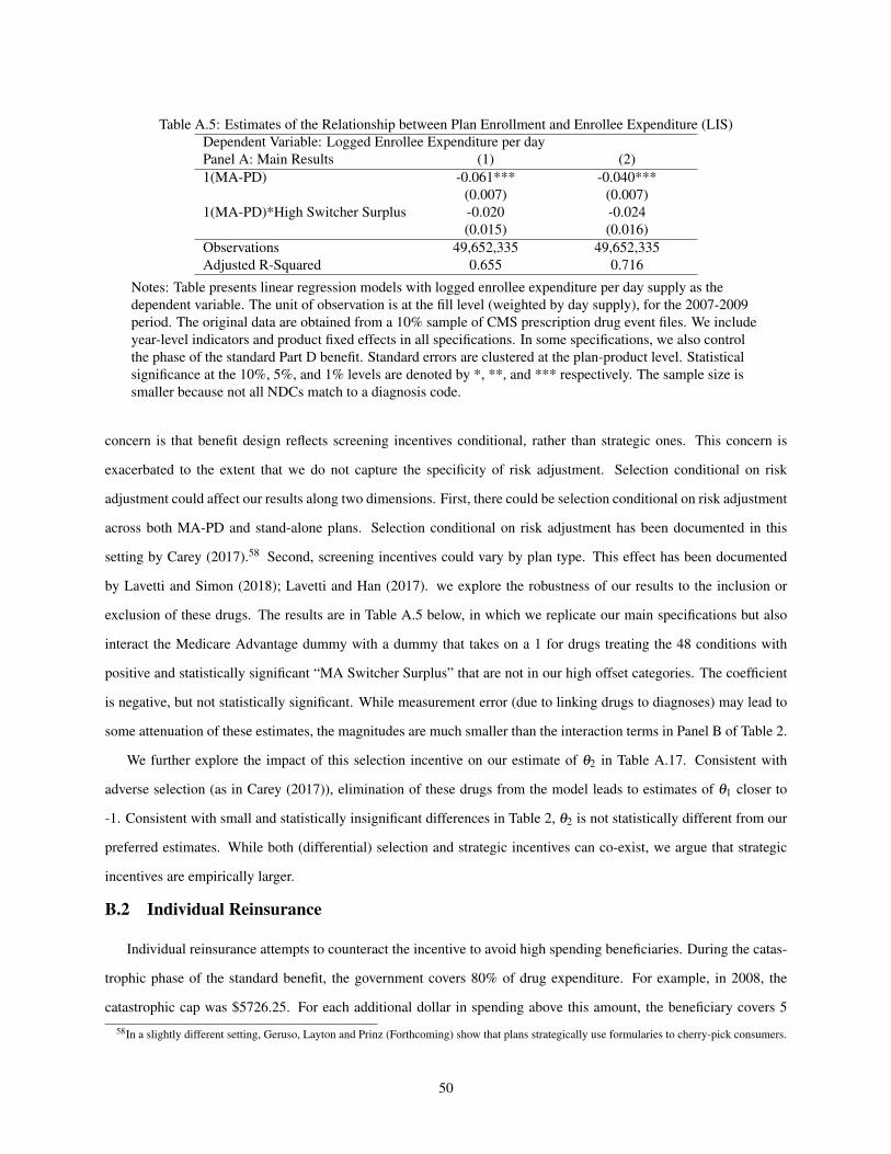
Table A.5: Estimates of the Relationship between Plan Enrollment and Enrollee Expenditure (LIS)Dependent Variable: Logged Enrollee Expenditure per dayPanel A: Main Results (1) (2)1(MA-PD) -0.061*** -0.040***

(0.007) (0.007)1(MA-PD)*High Switcher Surplus -0.020 -0.024

(0.015) (0.016)Observations 49,652,335 49,652,335Adjusted R-Squared 0.655 0.716

Notes: Table presents linear regression models with logged enrollee expenditure per day supply as thedependent variable. The unit of observation is at the fill level (weighted by day supply), for the 2007-2009period. The original data are obtained from a 10% sample of CMS prescription drug event files. We includeyear-level indicators and product fixed effects in all specifications. In some specifications, we also controlthe phase of the standard Part D benefit. Standard errors are clustered at the plan-product level. Statisticalsignificance at the 10%, 5%, and 1% levels are denoted by *, **, and *** respectively. The sample size issmaller because not all NDCs match to a diagnosis code.

concern is that benefit design reflects screening incentives conditional, rather than strategic ones. This concern is

exacerbated to the extent that we do not capture the specificity of risk adjustment. Selection conditional on risk

adjustment could affect our results along two dimensions. First, there could be selection conditional on risk adjustment

across both MA-PD and stand-alone plans. Selection conditional on risk adjustment has been documented in this

setting by Carey (2017).58 Second, screening incentives could vary by plan type. This effect has been documented

by Lavetti and Simon (2018); Lavetti and Han (2017). we explore the robustness of our results to the inclusion or

exclusion of these drugs. The results are in Table A.5 below, in which we replicate our main specifications but also

interact the Medicare Advantage dummy with a dummy that takes on a 1 for drugs treating the 48 conditions with

positive and statistically significant “MA Switcher Surplus” that are not in our high offset categories. The coefficient

is negative, but not statistically significant. While measurement error (due to linking drugs to diagnoses) may lead to

some attenuation of these estimates, the magnitudes are much smaller than the interaction terms in Panel B of Table 2.

We further explore the impact of this selection incentive on our estimate of θ2 in Table A.17. Consistent with

adverse selection (as in Carey (2017)), elimination of these drugs from the model leads to estimates of θ1 closer to

-1. Consistent with small and statistically insignificant differences in Table 2, θ2 is not statistically different from our

preferred estimates. While both (differential) selection and strategic incentives can co-exist, we argue that strategic

incentives are empirically larger.

B.2 Individual Reinsurance

Individual reinsurance attempts to counteract the incentive to avoid high spending beneficiaries. During the catas-

trophic phase of the standard benefit, the government covers 80% of drug expenditure. For example, in 2008, the

catastrophic cap was $5726.25. For each additional dollar in spending above this amount, the beneficiary covers 5

58In a slightly different setting, Geruso, Layton and Prinz (Forthcoming) show that plans strategically use formularies to cherry-pick consumers.

50

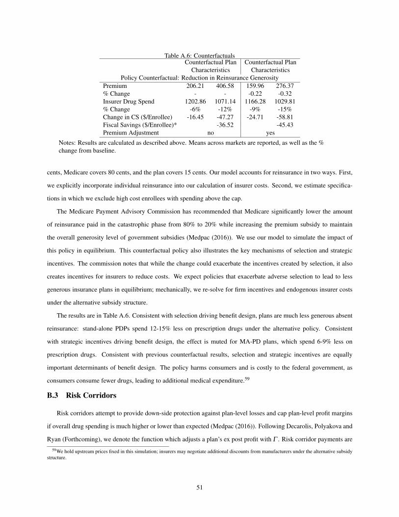
Table A.6: CounterfactualsCounterfactual Plan Counterfactual Plan

Characteristics CharacteristicsPolicy Counterfactual: Reduction in Reinsurance Generosity

Premium 206.21 406.58 159.96 276.37% Change - - -0.22 -0.32Insurer Drug Spend 1202.86 1071.14 1166.28 1029.81% Change -6% -12% -9% -15%Change in CS ($/Enrollee) -16.45 -47.27 -24.71 -58.81Fiscal Savings ($/Enrollee)* -36.52 -45.43Premium Adjustment no yes

Notes: Results are calculated as described above. Means across markets are reported, as well as the %change from baseline.

cents, Medicare covers 80 cents, and the plan covers 15 cents. Our model accounts for reinsurance in two ways. First,

we explicitly incorporate individual reinsurance into our calculation of insurer costs. Second, we estimate specifica-

tions in which we exclude high cost enrollees with spending above the cap.

The Medicare Payment Advisory Commission has recommended that Medicare significantly lower the amount

of reinsurance paid in the catastrophic phase from 80% to 20% while increasing the premium subsidy to maintain

the overall generosity level of government subsidies (Medpac (2016)). We use our model to simulate the impact of

this policy in equilibrium. This counterfactual policy also illustrates the key mechanisms of selection and strategic

incentives. The commission notes that while the change could exacerbate the incentives created by selection, it also

creates incentives for insurers to reduce costs. We expect policies that exacerbate adverse selection to lead to less

generous insurance plans in equilibrium; mechanically, we re-solve for firm incentives and endogenous insurer costs

under the alternative subsidy structure.

The results are in Table A.6. Consistent with selection driving benefit design, plans are much less generous absent

reinsurance: stand-alone PDPs spend 12-15% less on prescription drugs under the alternative policy. Consistent

with strategic incentives driving benefit design, the effect is muted for MA-PD plans, which spend 6-9% less on

prescription drugs. Consistent with previous counterfactual results, selection and strategic incentives are equally

important determinants of benefit design. The policy harms consumers and is costly to the federal government, as

consumers consume fewer drugs, leading to additional medical expenditure.59

B.3 Risk Corridors

Risk corridors attempt to provide down-side protection against plan-level losses and cap plan-level profit margins

if overall drug spending is much higher or lower than expected (Medpac (2016)). Following Decarolis, Polyakova and

Ryan (Forthcoming), we denote the function which adjusts a plan’s ex post profit with Γ . Risk corridor payments are

59We hold upstream prices fixed in this simulation; insurers may negotiate additional discounts from manufacturers under the alternative subsidystructure.

51

applied at the plan level at the end of the year (rather than enrollee by enrollee). Because payments are piece-wise

linear and symmetric, they do not affect the optimization of the risk neutral insurer. Therefore, we do not include risk

corridor payments in our discussion of firm profits in the main text. If we take risk corridor payments into account, the

ex post profit function can be written as:

ΠPDPjmt (b

Dt ,x

Dmt) = Γ

(pD

jmt(bDt )+ zD

t − cDjmt(x

Dmt, r jmt)

)s jmtBmt . (18)

Risk corridor payments are an important component of the program. Most plan sponsors returned a portion of over-

payments to Medicare because of the risk corridors. Despite being prevalent, industry participants are circumspect

about the impact of risk corridor payments on firm behavior (Medpac (2016)). The strongest incentives would be to

change bidding behavior; we do not use this information directly in estimation. To confirm that risk corridor payments

do not affect the parameter θ1, we re-estimate our model year by year, noting that the structure of risk corridors changed

in 2008. In unreported specifications, we find that the effect is not statistically different from the main specification.

B.4 Rebates and LIS Subsidies

Two additional features of the regulatory environment deserve additional attention: Medicare Advantage rebates

and LIS subsidies. Because Medicare Advantage subsidies were generous during our time period, many plans have

zero premiums; these plans may include “rebates” to enrollees, which can be used to provide additional services or

reduce Part B premiums (which are required even for consumers in Medicare Advantage plans).We include these net

premium reductions directly in the definition of bMjmt ; the consumer pays a composite premium equal to bM

jmt + pDjmt .

We can allow the value of the rebate to be reduced by 25% in accordance with CMS bidding rules, which require that

the government share in the savings of Medicare Advantage plans that bid below the benchmark. Table A.17 shows

that this will not affect the estimates of the key parameters of interest.

Second, distortions created by the LIS subsidy may affect firm incentives. Decarolis, Polyakova and Ryan (Forth-

coming) account for this possibility in their analysis and we following their approach by restricting attention to those

contracts that bid above the LIS benchmark amount in the majority of regions in which they operate. We re-estimate

the supply-side parameters, assuming that these remaining contracts will not be distorted by the structure of the LIS

subsidy. This restriction leaves fewer contracts available to estimate the parameters. Nevertheless, the results (pre-

sented in Table A.17) are qualitatively similar to the main specification, indicating that our basic results hold even

allowing for the LIS distortion. Similarly, in the bottom panel of Table A.17, we restrict attention to “enhanced” plans

that are unlikely to be constrained by minimum plan generosity requirements; again, the results are quantitatively

similar.60

60We define a plan as “enhanced” if it has a supplemental premium in at least half of all markets in which it operates. This accounts for 7% ofall stand-alone plans. The analysis omitting LIS plans serves as an additional robustness check along this dimension as plans not eligible for LISenrollment are also likely to be more generous than the minimum actuarial standard. These two subsets overlap substantially.

52

C Additional Counterfactuals

In this section, we consider a number of policy-relevant counterfactuals. In all of these exercises, we assume fixed

θ1 and θ2. For example, we consider budget neutral policies that attempt to internalize the externality generated by

the stand-alone PDPs.61 Our presumption is that CMS would like to increase drug consumption by PDP enrollees

to both improve enrollee well-being and to reduce medical care costs. A natural policy to consider is a plan benefit

generosity subsidy where CMS would cover some of the insurer’s cost to increase generosity. For this subsidy to

be budget neutral, CMS must also decrease the current premium subsidy, which will likely increase premiums faced

by consumers. The impact of such a change depends on how consumers evaluate plans with greater generosity but

higher premiums. While it is natural to consider the consumer surplus impact of these policies, such a calculation

requires interpreting the utility parameters in the neoclassical context, which, given our earlier findings, is probably

inappropriate. For this reason, we refrain from making consumer surplus statements here. In addition, we assume

fixed θ1 and θ2 in all of the policy counterfactuals.

Consider a uniform subsidy for stand-alone PDPs, as shown in Table A.7. Mechanically, a subsidy alters both p jmt

and OOPCq jmt if it is budget neutral and there is full pass-through; we can write the alternative premium and OOPC as

a function of the change in OOPC due to a change in the benefit generosity and the offset, which is given by ∂q∂x (c−c′).

For a small change in x (omitting subscripts for simplicity):

OOPC′ = OOPC+∂OOPC

∂x,

p′ = p+∂OOPC

∂x− ∂q

∂x(c− c′).

In this formulation, the offset savings are passed through completely to the consumer in the form of lower premiums,

but the reduced premium subsidy is passed through to consumers in the form of higher premiums as well.62

A 1% subsidy would increase consumption by 7.2 day supply based on the behavioral elasticities in column 2. The

implied offset, in column 3, is $3.54.63 However, the subsidy applies to all of the infra-marginal units as well, and

the total reduction in OOPC is $10.15. Subtracting the offsets, this implies that premiums would have to increase by

$6.61 for the policy to be budget neutral. By contrast, the federal government could eliminate cost-sharing in the donut

hole, as the ACA does. Using the calculations in Einav, Finkelstein and Schrimpf (2015), this would increase drug

consumption by 8%, generating offsets amounting to $52.54 per consumer. However, this policy is also expensive:

while it reduces OOPC by $356 per consumer, this reduction comes at a cost net of offsets of $303. Therefore, if the

61These calculations do not require knowledge of the “true” demand curve, from which we could derive welfare implications as in Glazer andMcGuire (2013).

62This gives us an upper bound of the potential welfare gain.63This is calculated as the additional spending multiplied by the 22% figure described above.

53

Tabl

eA

.7:C

ount

erfa

ctua

lPol

icie

sU

nifo

rmE

last

icity

Off

set

Cha

nge

inO

OPC

Eff

ectiv

eC

ost

%C

hang

e,C

onsu

mer

Val

uatio

n,O

OPC

Red

uctio

n(t

oG

over

nmen

t)PD

PPe

netr

atio

nO

OPC

Red

uctio

n(U

B)

1.00

%-0

.54

3.54

10.1

56.

61-0

.001

04.

302.

50%

-0.3

86.

2325

.28

19.0

6-0

.003

010

.70

5.00

%-0

.33

10.8

250

.51

39.6

9-0

.006

421

.38

10.0

0%-0

.30

19.6

710

0.94

81.2

8-0

.013

242

.74

25.0

0%-0

.29

47.5

325

2.30

204.

77-0

.034

210

6.82

50.0

0%-0

.29

95.0

650

4.60

409.

54-0

.074

421

3.64

75.0

0%-0

.31

152.

4375

7.27

604.

84-0

.122

432

0.61

Elim

inat

eth

eD

onut

Hol

e52

.435

5.99

303.

58-0

.057

115

2.86

Not

es:R

esul

tsar

eca

lcul

ated

asde

scri

bed

inSe

ctio

n5.

54

policy is to be budget neutral, premiums will have to rise dramatically.64

Furthermore, these policies reduce the market share of stand-alone PDPs. Consumers do not value the increased

generosity at its full cost, as reflected in the measured decision utility; they prefer plans with lower premiums and

higher cost-sharing. Therefore, we conclude that it will be difficult for the government to implement broad based

changes to the Part D program aimed at reducing externalities that are budget neutral. This includes the recent Part

D Enhanced Medication Therapy Management (MTM) Model, which encourages stand-alone plans to reduce Parts A

and B spending among their enrollees. The actual financial incentives associated with this program are quite small.

If plans reduce Parts A and B spending by 2% (about $200 in 2008), they are eligible for a $2 per member per

month increase in their benchmark payment. Because firms only receive approximately one-tenth of the savings, they

are unlikely to internalize the externality created by offsets. Furthermore, we note that a stand-alone PDP that fully

internalized the externality would only spend an additional $153 per enrollee per year. Given our calculations, this

would lead to savings in Parts A and B of about $30. We find that a policy that provides a $12.75 per member per

month increase in the benchmark payment (and reduces Parts A and B spending by 0.3%) internalizes the externality,

and would increase MA-PD enrollment by 3.4 percentage points. Furthermore, we note that a $153 increase is likely

to represent the insurers’ entire profit margins, based on a 15% profit margin and the estimates in Ho, Hogan and

Scott Morton (2015).

It is costly for the Medicare program to implement a budget neutral policy for two reasons: consumers are not

sophisticated with respect to potential under-utilization and most implementable policies fail to target marginal con-

sumption, effectively leading to expensive OOPC reductions on infra-marginal units. These results are consistent with

a model in which private insurers can better target and subsidize underutilized, high-value care. For example, while

the subsidy we describe is uniform, applying to all drugs, private MA-PD insurers can implement more sophisticated

contracts that better target increased utilization. We see evidence of this in the reduced form results; MA-PD plans

have lower enrollee expenditure for exactly those drugs likely to generate the largest offsets. While they increase the

complexity of insurance contracts and may exacerbate plan choice frictions, targeted subsidies are more likely to be

cost-effective. Therefore, it may be more reasonable to encourage MA-PD enrollment; based on our estimates in Table

4, we believe this can be done in a cost-effective way. For example, rather than closing the donut hole, the federal

government could increase Medicare Advantage benchmarks by $312 per year, plus the $23 in implied offsets. This

would increase MA-PD market share by 7.4%.

By contrast, market outcomes could be very different absent choice frictions. In the main demand specifications,

we allow for inertia and do not constrain αpq = αx

q . Incorporating deviations from the neoclassical model builds on

previous work (Ho, Hogan and Scott Morton (2015); Abaluck and Gruber (2016); Decarolis, Polyakova and Ryan

64Exacerbating this is the fact that MA-PD plans become more generous in equilibrium, decreasing OOPC to consumers by $97 per year. Wenote that the ACA policy is not budget neutral.

55

Table A.8: IV Nested Logit Parameter EstimatesRisk Quintile (Lowest to Highest) (1) (2) (3) (4) (5)Premium + OOPC -0.157*** -0.119*** -0.0887*** -0.0581*** -0.0248***

(0.00610) (0.00508) (0.00439) (0.00355) (0.00242)1−σ 0.439*** 0.441*** 0.470*** 0.463*** 0.457***

(0.0132) (0.0134) (0.0130) (0.0127) (0.0119)Plan Vintage 2.148*** 1.466** -2.177 0.437 0.592

(0.631) (0.630) (13,226) (0.630) (0.632)Adjusted R2 0.308 0.294 0.291 0.285 0.271Observations 58,189 58,626 59,885 60,463 61,317

Notes: Table presents instrumental variable regression models as described in Berry (1994). The outsideshare is constructed as all Medicare eligibles not enrolled in a stand-alone Medicare Part D plan or MA-PDplan. In all specifications, we include plan fixed effects. Excluded instruments are an urban county dummy,and premiums and out-of-pocket expenditure in other markets, where a market is defined as a county-yearcombination. Standard errors are presented in parentheses. Statistical significance at the 10%, 5%, and 1%levels are denoted by *, **, and *** respectively.

(Forthcoming)) and is important for understanding insurer incentives. However, a natural approach would assume

that consumers care equally about a dollar reduction in premium and a dollar reduction in OOPC. In Table A.8, we

present results that constrain αpq = αx

q . Consistent with the patterns in our main specifications, sicker consumers are

less sensitive to the combination of premiums and OOPC.

We next consider the impact of consumer decision making in equilibrium. To align consumer choices with value,

policymakers could provide targeted consumer search tools (Handel and Kolstad (2015)). In this setting, we believe

that would lead consumers to place greater weight on OOPC (Ericson and Starc (2016)) and lead to reduced naivete

about potential under-consumption. Mechanically, we resolve for optimal insurer costs assuming the demand specifi-

cation in Table A.8, such that consumers treat a $1 increase in premiums equal to a $1 increase in OOPC. The results

are in the final two columns of the top panel of Table A.9. If consumers were "sophisticated," plans would increase

their generosity. MA-PD plans would spend 6% more on prescription drugs, while stand-alone PDPs would spend 4%

more. Public policies that align consumer demand or the structure of subsidies with providing value will lead insurers

to offer contracts that reduce costs or increase health.

We perform two additional counterfactuals to explore the extent to which other features of the institutional environ-

ment affect market outcomes. First, we estimate our main counterfactual using our baseline demand estimates, which

do not account for plan vintage and imply substantially less adverse selection. In this counterfactual, stand-alone PDPs

are much more generous than in the preferred estimates. This implies that accounting for inertia is critical and that

selection – in addition to strategic incentives – plays an important role in benefit design.

Finally, we explore the effect of imperfect competition on benefit design and premium setting. We estimate a

counterfactual in which plans are constrained to pay out 80% of the premiums they collect in (drug) claims, known as

a (binding) minimum loss ratio regulation. The regulation (enacted as part of the Affordable Care Act) is essentially

56

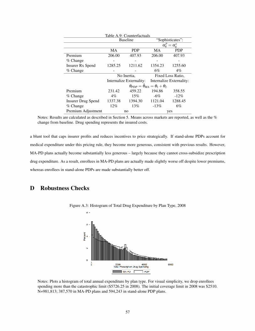
Table A.9: CounterfactualsBaseline “Sophisticates”:

αpq = αx

qMA PDP MA PDP

Premium 206.00 407.93 206.00 407.93% Change - - - -Insurer Rx Spend 1285.25 1211.62 1354.23 1255.60% Change - - 6% 4%

No Inertia, Fixed Loss Ratio,Internalize Externality: Internalize Externality:

θPDP = θMA = θ1 +θ2Premium 231.42 459.22 194.86 358.55% Change 4% 15% -6% -12%Insurer Drug Spend 1337.38 1394.30 1121.04 1288.45% Change 12% 13% -13% 6%Premium Adjustment no yes

Notes: Results are calculated as described in Section 5. Means across markets are reported, as well as the %change from baseline. Drug spending represents the insured costs.

a blunt tool that caps insurer profits and reduces incentives to price strategically. If stand-alone PDPs account for

medical expenditure under this pricing rule, they become more generous, consistent with previous results. However,

MA-PD plans actually become substantially less generous – largely because they cannot cross-subsidize prescription

drug expenditure. As a result, enrollees in MA-PD plans are actually made slightly worse off despite lower premiums,

whereas enrollees in stand-alone PDPs are made substantially better off.

D Robustness Checks

Figure A.3: Histogram of Total Drug Expenditure by Plan Type, 2008

Notes: Plots a histogram of total annual expenditure by plan type. For visual simplicity, we drop enrolleesspending more than the catastrophic limit ($5726.25 in 2008). The initial coverage limit in 2008 was $2510.N=981,813; 387,570 in MA-PD plans and 594,243 in stand-alone PDP plans.

57

Figure A.4: Effects by Drug Class

-.1-.0

50

.05

.1ln

(OO

PC p

er d

ay)

All Beta Blockers OtherType of Hypertension Drug

Notes: This figure plots the differences in prices by plan type. Other hypertension drugs include ACEinhibitors, angiotensin II receptor antagonists, renin inhibitors, antiadrenergic agents (centrally &peripherally acting), alpha-adrenergic blockers, aldosterone receptor antagonists, vasodilators andantihypertensive combination therapies. Standard errors are clustered at the plan-product level.

Figure A.5: Supply-Side Identification

Notes: This figure plots the optimal level of insurer spending under alternative levels of θ from first-orderconditions from both xICR and xDonut , using average values of the derivatives of shares with respect topremiums and out-of-pocket costs.

58

Table A.10: Estimates of the Relationship between Plan Enrollment and Enrollee Expenditure, No Third Party Pay-ments

Dependent Variable: Logged Enrollee Expenditure per dayPanel A: Main Results (1) (2)1(MA-PD) -0.042*** -0.019***

(0.003) (0.004)Observations 119,915,976 119,915,976Adjusted R-Squared 0.655 0.729Panel B: By High Offset Class1(MA-PD) -0.036*** -0.015**

(0.005) (0.005)1(MA-PD)*Asthma -0.088*** -0.102***

(0.018) (0.018)1(MA-PD)*Hypertension 0.033*** 0.042***

(0.009) (0.009)1(MA-PD)*Diabetes -0.035*** -0.034**

(0.010) (0.011)1(MA-PD)*Cholesterol -0.067*** -0.064***

(0.009) (0.010)Observations 119,915,976 119,915,976Adjusted R-Squared 0.655 0.729Product Fixed Effects X XPhase Fixed Effects X

ICR or DeductiblePanel C: By Benefit Phase (Ded Amt. = 0) Donut Hole1(MA-PD) 0.032*** -0.266***

(0.004) (0.004)Observations 94,800,906 16,301,087Adjusted R-Squared 0.731 0.730

Notes: Table presents linear regression models with logged enrollee expenditure per day supply as thedependent variable. The unit of observation is at the fill level (weighted by day supply), for the 2007-2009period. The original data are obtained from a 10% sample of CMS prescription drug event files. We includeyear-level indicators and product fixed effects in all specifications. In some specifications, we also controlthe phase of the standard Part D benefit. Standard errors are clustered at the plan-product level. Statisticalsignificance at the 10%, 5%, and 1% levels are denoted by *, **, and *** respectively.

59

Table A.11: Estimates of the Relationship between Plan Enrollment and Enrollee ExpenditureDependent Variable: Enrollee Expenditure per day

(1) (2)1(MA-PD) -0.050*** -0.029***

(0.003) (0.004)1(day supply < 30) 0.444*** 0.434***

(0.007) (0.007)1(day supply 31-90) -0.181*** -0.177***

(0.003) (0.003)1(day supply > 90 -0.107*** -0.099***

(0.025) (0.026)Observations 123,031,165 123,031,165Adjusted R-Squared 0.631 0.698Product Fixed Effects X XPhase Fixed Effects X

Notes: Table presents linear regression models with logged enrollee expenditure per day supply as thedependent variable. The unit of observation is at the fill level (weighted by day supply), for the 2007-2009period. The original data are obtained from a 10% sample of CMS prescription drug event files. We includeyear-level indicators and product fixed effects in all specifications. In some specifications, we also controlthe phase of the standard Part D benefit. Standard errors are clustered at the plan-product level. Thirty daysupply prescriptions (the most common) is the omitted category. Statistical significance at the 10%, 5%, and1% levels are denoted by *, **, and *** respectively.

Table A.12: Mechanisms(1) (2)

Panel A: Main Results Outcome: 1(90 Day)1(MA-PD) 0.00272** 0.00212*

(0.000929) (0.000939)Observations 153,964,560 153,964,560Adjusted R-Squared 0.096 0.097Panel B: Main Results Outcome: Total Cost/Day1(MA-PD) -0.00955 -0.00468

(0.00656) (0.00657)Observations 153,962,060 153,962,060Adjusted R-Squared 0.590 0.590

Notes: Table presents linear regression models, where outcome variables are as described in each panel. Theunit of observation is at the fill level, for the 2007-2009 period. The original data are obtained from a 10%sample of CMS prescription drug event files. We include year-level indicators and product fixed effects inall specifications. In some specifications, we also control the phase of the standard Part D benefit. Standarderrors are clustered at the plan-product level. Statistical significance at the 10%, 5%, and 1% levels aredenoted by *, **, and *** respectively.

60

Table A.13: Benefit Design and Out-of-Pocket CostsDependent Variable: Out-of-Pocket Costs

(1) (2) (3) (4) (5) (6)xICR

jmt 501.5*** 638.9*** 499.7*** 640.6*** 498.8*** 637.3***(49.05) (56.45) (48.86) (56.44) (48.53) (55.80)

xDonutjmt -2.442 5.911 -2.129 5.160 -1.758 6.468

(9.377) (18.19) (9.311) (18.22) (9.293) (18.12)1(MA)∗ xICR

jmt -291.4*** -291.2*** -289.8***(72.49) (72.94) (71.88)

1(MA)∗ xDonutjmt -6.640 -6.057 -6.916

(16.54) (16.53) (16.52)FFS Costs 0.281*** 0.281***

(0.0358) (0.0357)R-Squared 0.228 0.230 0.230 0.228 0.230 0.231Observations 569,078 569,078 569,078 569,078 569,078 569,078Year FE X X X X X XRisk Type FE X X X X X XDemo. Controls X X X XPlan FE X X X X X X

Notes: Table presents OLS regression models, where outcome variable is consumer out-of-pocket costs. Theunit of observation is an enrollee-year for the 2007-2009 period. The original data are obtained from a 10%sample of CMS prescription drug event files, aggregated to the enrollee-year level. We include year-levelindicators and indicators for the quintile of 2006 spending (consumer types) in all specifications. In somespecifications, we also control for 5-year average per capita Medicare FFS spending and demographiccontrols for age categories, race, and gender. Standard errors are clustered at the contract level and arepresented in parentheses. Statistical significance at the 10%, 5%, and 1% levels are denoted by *, **, and*** respectively.

61

Tabl

eA

.14:

IVN

este

dL

ogit

Res

ults

Ris

kQ

uint

ile(L

owes

tto

Hig

hest

)(1

)(2

)(3

)(4

)(5

)Pr

oduc

tCha

ract

eris

tics

App

roac

hPr

emiu

m-0

.032

6***

-0.0

518*

**-0

.063

3***

-0.0

626*

**-0

.052

6***

(0.0

0671

)(0

.006

94)

(0.0

0732

)(0

.007

32)

(0.0

0634

)D

onut

Hol

eC

over

age

0.99

7***

1.11

5***

1.69

7***

1.95

7***

1.68

8***

(0.0

953)

(0.0

896)

(0.0

985)

(0.0

989)

(0.0

897)

Has

Ded

uctib

le-1

.036

***

-1.0

50**

*-1

.174

***

-1.2

13**

*-1

.054

***

(0.0

328)

(0.0

332)

(0.0

356)

(0.0

360)

(0.0

325)

Plan

Vin

tage

0.39

4***

0.45

3***

0.44

3***

0.46

9***

0.49

0***

(0.0

209)

(0.0

222)

(0.0

237)

(0.0

250)

(0.0

241)

1−

σ0.

318*

**0.

343*

**0.

374*

**0.

384*

**0.

376*

**(0

.011

0)(0

.011

1)(0

.011

4)(0

.011

6)(0

.010

3)O

bser

vatio

ns58

,189

58,6

2659

,885

60,4

6361

,317

Adj

uste

dR

-Squ

ared

0.37

80.

356

0.25

10.

173

0.24

2

Not

es:O

urcu

rren

tapp

roac

hre

lies

onpl

anfix

edef

fect

san

did

entifi

esse

nsiti

vity

topr

ice

and

OO

PCus

ing

cros

sm

arke

tvar

iatio

n.To

addr

ess

the

role

ofse

lect

ion

inth

ede

term

inat

ion

ofco

ntra

ctch

arac

teri

stic

sm

ore

dire

ctly

,we

mod

elpl

anch

oice

asa

func

tion

ofco

ntra

ctch

arac

teri

stic

s.In

thes

esp

ecifi

catio

ns,w

ein

clud

epr

emiu

ms,

OO

PC,a

nddu

mm

ies

ford

educ

tible

and

donu

thol

eco

vera

geas

the

obse

rvab

lech

arac

teri

stic

s.Ta

ble

pres

ents

inst

rum

enta

lvar

iabl

ere

gres

sion

mod

els,

whe

reth

eou

tcom

eva

riab

leis

the

log

ofth

epl

ansh

are

less

the

log

ofth

eou

tsid

esh

are.

The

outs

ide

shar

eis

cons

truc

ted

asal

lMed

icar

eel

igib

les

note

nrol

led

ina

stan

d-al

one

Med

icar

ePa

rtD

plan

orM

A-P

Dpl

an.W

ein

clud

epl

anfix

edef

fect

sin

alls

peci

ficat

ions

.In

stru

men

tsar

eth

eur

ban

dum

my,

asw

ella

spr

emiu

ms

and

out-

of-p

ocke

tcos

tsin

othe

rmar

kets

,whe

rea

mar

keti

sde

fined

asa

coun

ty-y

earc

ombi

natio

n.St

atis

tical

sign

ifica

nce

atth

e10

%,5

%,a

nd1%

leve

lsar

ede

note

dby

*,**

,and

***

resp

ectiv

ely.

62

Tabl

eA

.15:

Uno

bser

ved

Dem

and

Het

erog

enei

tyR

isk

Qui

ntile

(Low

estt

oH

ighe

st)

(1)

(2)

(3)

(4)

(5)

Bas

elin

eM

odel

Prem

ium

,Typ

e1

-0.1

391

-0.1

275

-0.0

831

-0.0

897

-0.0

940

(0.0

178)

(0.0

053)

(0.0

085)

(0.0

071)

(0.0

303)

OO

PC,T

ype

1-0

.112

3-0

.064

9-0

.043

5-0

.024

24-0

.059

1(0

.016

7)(0

.023

6)(0

.003

1)(0

.003

0)(0

.006

1)Pr

emiu

m,T

ype

2-0

.232

5-0

.222

8-0

.254

8-0

.249

5-0

.284

5(0

.016

7)(0

.010

4)(0

.010

7)(0

.008

4)(0

.055

0)O

OPC

,Typ

e2

-0.1

263

-0.0

826

-0.0

486

-0.0

303

-0.0

159

(0.0

112)

(0.0

088)

(0.0

044)

(0.0

035)

(0.0

043)

γ(%

ofTy

pe2)

0.65

530.

6617

0.66

800.

6740

0.61

08(0

.049

8)(0

.001

8)(0

.033

0)(0

.024

0)(0

.134

2)A

llow

ing

forI

nert

iaPr

emiu

m,T

ype

1-0

.141

5-0

.144

5-0

.131

6-0

.132

0-0

.112

0(0

.026

1)(0

.024

3)(0

.022

2)(0

.020

6)(0

.019

5)O

OPC

,Typ

e1

-0.0

965

-0.0

516

-0.0

298

-0.0

139

0.00

10(0

.013

4)(0

.010

5)(0

.007

6)(0

.000

5)(0

.003

4)Pr

emiu

m,T

ype

2-0

.174

9-0

.171

7-0

.198

0-0

.191

7-0

.193

0(0

.051

6)(0

.051

9)(0

.052

3)(0

.053

2)(0

.055

4)O

OPC

,Typ

e2

-0.1

199

-0.0

774

-0.0

435

-0.0

267

-0.0

007

(0.0

261)

(0.0

243)

(0.0

222)

(0.0

344)

(0.0

039)

Plan

Vin

tage

0.76

880.

7456

0.63

000.

6390

0.77

79(0

.057

8)(0

.062

3)(0

.065

4)(0

.070

4)(0

.084

3)γ

(%of

Type

2)0.

6553

0.66

170.

6680

0.67

400.

6799

(0.2

198)

(0.2

080)

(0.2

288)

(1.7

229)

(0.2

886)

Not

es:O

urcu

rren

tapp

roac

hal

som

odel

she

tero

gene

ityin

dem

and

acro

ssob

serv

able

,but

notu

nobs

erva

ble

cons

umer

char

acte

rist

ics.

We

argu

eth

at,g

iven

both

the

empi

rica

llite

ratu

rean

dre

duce

dfo

rmre

sults

,we

incl

ude

mos

toft

heva

riat

ion

acro

ssco

nsum

ers

that

ispr

edic

tabl

eto

insu

rers

.How

ever

,am

ore

flexi

ble

dem

and

syst

emm

aybe

tterc

aptu

reth

epa

ttern

sof

subs

titut

ion

inth

eda

ta.W

ere

port

estim

ates

that

allo

wfo

ra

mix

ture

ofun

obse

rved

cons

umer

type

s,si

mila

rto

Ber

ryan

dJi

a(2

010)

.The

resu

ltsar

equ

alita

tivel

ysi

mila

rto

the

mai

nes

timat

es,t

houg

hth

eyim

ply

slig

htly

less

sens

itivi

tyam

ong

high

spen

ders

.For

num

eric

alst

abili

ty,m

arke

tsw

ithle

ssth

an50

,000

enro

llees

wer

edr

oppe

dfr

omth

ean

alys

is.I

nTa

ble

A.1

7,w

esh

owth

atou

rsup

ply-

side

estim

ates

are

nots

ensi

tive

the

incl

usio

nof

addi

tiona

lcon

sum

erhe

tero

gene

ity.

Star

sde

notin

gsi

gnifi

canc

eom

itted

.

63

Table A.16: Supply Side Incentive and Inertia(1) (2) (3)

Panel A, Dep. Var.: Logged PremiumsLagged Market Share 0.855*** 0.902***

(0.00453) (0.00465)Enrollment Growth Rate -0.00281 -0.0846***

(0.00180) (0.00187)N 2,174,111 2,174,111 2,174,111Panel B, Dep. Var.: Logged Insurer CostsLagged Market Share 0.0103 0.0131

(0.0142) (0.0143)Enrollment Growth Rate -0.0182** -0.0186**

(0.00603) (0.00615)N 3,022,704 3,022,704 3,022,704

Notes: The unit of observation is the beneficiary year. All specifications include contract, state, and yearfixed effects. Statistical significance at the 10%, 5%, and 1% levels are denoted by *, **, and ***respectively.

Table A.17: Supply Results(1) (2) (3) (4) (5) (6) (7) (8)Multi-Product Unobserved Non-LIS Basic

Firms Heterogeneity Distorted Plansθ1 -0.9729 -1.2798 -0.9714 -1.3427 -1.1871 -1.3376 -0.9761 -1.3427

(0.0082) (0.0080) (0.0081) (0.0079) (0.0081) (0.0082) (0.0154) (0.0163)θ2 0.3491 0.4211 0.3814 0.2584

(0.0301) (0.0304) (0.0411) (0.0333)N 33,538 33,538 33,538 33,538 13,737 13,737 28,975 28,975

(9) (10) (15) (16) (11) (12) (13) (14)Alt. Fixed xICR

jmt FinerRebate Markup Only Risk Adj.

θ1 -1.0481 -1.3427 -0.9401 -1.3427 -0.5762 -0.8020 -0.8827 -1.1562(0.0065) (0.0378) (0.0082) (0.0078) (0.0046) (0.0045) (0.0101) (0.0093)

θ2 0.3341 0.4565 0.2559 0.3010(0.0397) (0.0310) (0.0173) (0.0469)

N 33,538 33,538 33,538 33,538 33,538 33,538 33,538 33,538

Notes: Parameters are estimated using generalized method of moments as described in Section 4. Standarderrors are calculated using a bootstrap that re-samples plans with replacement. Observations are at theplan-market-year level. Models (1) and (2) allow firms to optimize over their full portfolio of plans, whilemodels (3) and (4) incorporate unobserved demand heterogeneity as described in Table A.15. Models(5)-(8) restrict the sample of plans used in the analysis. Models (9)-(16) test robustness to alternative costassumptions described in the text. Models (11) and (12) set xD

jmt = xICRjmt , and Models (13) and (14) exclude

drugs identified by Lavetti and Simon (2018) and Lavetti and Han (2017) to lead to differential selection byplan type.

64