Extension technique for complete Bernstein functions of the … · Mateusz Kwa´snicki and Jacek Mucha Abstract. We discuss the representation of certain functions of the Laplace

J. Evol. Equ. 18 (2018), 1341–1379© 2018 The Author(s)1424-3199/18/031341-39, published onlineMarch 15, 2018https://doi.org/10.1007/s00028-018-0444-4

Journal of EvolutionEquations

Extension technique for completeBernstein functions of theLaplaceoperator

Mateusz Kwasnicki and Jacek Mucha

Abstract. We discuss the representation of certain functions of the Laplace operator � as Dirichlet-to-Neumann maps for appropriate elliptic operators in half-space. A classical result identifies (−�)1/2, thesquare root of the d-dimensional Laplace operator, with the Dirichlet-to-Neumann map for the (d + 1)-dimensional Laplace operator �t,x in (0, ∞) × Rd . Caffarelli and Silvestre extended this to fractionalpowers (−�)α/2, which correspond to operators ∇t,x (t1−α∇t,x ). We provide an analogous result for allcomplete Bernstein functions of −� using Krein’s spectral theory of strings. Two sample applications areprovided: a Courant–Hilbert nodal line theorem for harmonic extensions of the eigenfunctions of non-localSchrödinger operators ψ(−�) + V (x), as well as an upper bound for the eigenvalues of these operators.Here ψ is a complete Bernstein function and V is a confining potential.

1. Introduction

Aclassical result identifies theDirichlet-to-Neumann operator in half-spacewith thesquare root of the Laplace operator; namely, if u(t, x) is harmonic inH = (0,∞)×Rd

with boundary value f (x) = u(0, x), then given some boundedness condition on u,we have

−(−�)1/2 f (x) = ∂t u(0, x).

The above observation was extended to general fractional powers of the Laplace oper-ator by Caffarelli and Silvestre in [5]: for α ∈ (0, 2), if u satisfies the elliptic equation

∇t,x (t1−α∇t,x u(t, x)) = 0 (1.1)

in H with boundary value f (x) = u(0, x), then under appropriate boundedness as-sumption on u, we have

−(−�)α/2 f (x) = |�(−α2 )|

α2α�(α2 )

limt→0+ t1−α∂t u(t, x)

= |�(−α2 )|

2α�(α2 )

limt→0+

u(t, x) − u(0, x)

tα.

(1.2)

Mathematics Subject Classification: Primary 35J25, 35J70, 47G20; Secondary 60J60, 60J75Keywords: Extension technique, Fractional Laplacian, Non-local operator, Complete Bernstein function,

Krein’s string.This work was supported by the Polish National Science Centre (NCN) Grant No. 2015/19/B/ST1/01457.

http://crossmark.crossref.org/dialog/?doi=10.1007/s00028-018-0444-4&domain=pdf

1342 M. Kwasnicki and J. Mucha J. Evol. Equ.

Noteworthy, the above extension dates back to the paper of Molchanov and Ostro-vski [44] within the probabilistic context, and it has been used by other authors beforethe work of Caffarelli and Silvestre; see, for example, [10,25,43]. Nevertheless, therepresentation (1.2) of the fractional Laplace operator was first given explicitly onlyin [5] and it is known as the Caffarelli–Silvestre extension technique. It is most com-monly applied in the setting of L 2 spaces, but versions for other Banach spaces oroperators are also available, see [2,22,49]. In fact, the above technique works for frac-tional powers of essentially arbitrary non-negative self-adjoint operators. For a briefdiscussion and further properties, we refer to Section 2.8 in [39].As a consequence of Krein’s spectral theory of strings, if the weight t1−α in (1.1)

is replaced by a more general function a(t), then the corresponding Dirichlet-to-Neumann operator is again a function of −�, say ψ(−�), and furthermore, ψ is acomplete Bernstein function. Conversely, any complete Bernstein function of −� canbe represented in this way, if one allows for certain singularities of a(t). Even thoughthismethod has already beenmentioned in the literature (see, for example, [21,37,51]),finding a reference is problematic.Themain purpose of this article is to fill in this gap and discuss rigorously the above-

mentioned general extension technique. This is complemented by two applicationsfor non-local Schrödinger operators ψ(−�) + V (x): a Courant–Hilbert theorem onnodal domains (for the extension problem), and an upper bound for the eigenvalues.For simplicity, we focus onL 2(Rd) results, although a more general approach seemsto be possible.Our results provide an answer to the question posed by Caffarelli and Silvestre

in the last paragraph of [5]: we characterise all operators that arise as Dirichlet-to-Neumann maps for local operators in half-space H with coefficients depending onthe first coordinate only. We also prove uniqueness of harmonic extensions, givenappropriate boundedness condition; the first result of this kind was proved in [49] forfractional powers of certain elliptic operators.We remark that the extension technique can also be generalised in different direc-

tions. For example, higher-order powers of −� can be studied in a somewhat similarway, see [7,23,46,50]. Furthermore, in [18] a closely related, but essentially differentextension technique is developed in a non-commutative setting, for the sub-Laplacianon the Heisenberg group.

1.1. Extension technique

If ψ is a function on [0,∞), by ψ(−�) we understand the Fourier multiplier onL 2(Rd) with symbol ψ(|ξ |2), that is, the operator

ψ(−�) f = F−1(ψ(| · |2)F f (·)). (1.3)

HereF denotes the Fourier transform and f is in the domain D(ψ(−�)) of ψ(−�)

if both f (ξ) and ψ(|ξ |2)F f (ξ) are in L 2(Rd). Our goal is to identify the operator

Vol. 18 (2018) Extension technique for complete Bernstein functions 1343

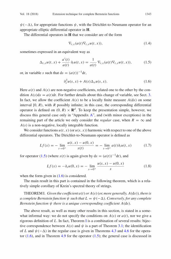
ψ(−�), for appropriate functions ψ , with the Dirichlet-to-Neumann operator for anappropriate elliptic differential operator in H.The differential operators in H that we consider are of the form

∇t,x (a(t)∇t,x u(t, x)), (1.4)

sometimes expressed in an equivalent way as

�t,x u(t, x) + a′(t)a(t)

∂t u(t, x) = 1

a(t)∇t,x (a(t)∇t,x u(t, x)), (1.5)

or, in variable s such that ds = (a(t))−1dt ,

∂2s u(s, x) + A(s)�x u(s, x). (1.6)

Here a(t) and A(s) are non-negative coefficients, related one to the other by the con-dition A(s)ds = a(t)dt . For further details about this change of variable, see Sect. 3.In fact, we allow the coefficient A(s) to be a locally finite measure A(ds) on someinterval [0, R), with R possibly infinite; in this case, the corresponding differentialoperator is defined on (0, R) × Rd . To keep the presentation simple, however, wediscuss this general case only in “Appendix A”, and (with minor exceptions) in theremaining part of the article we only consider the regular case, when R = ∞ andA(s) is a non-negative, locally integrable function.We consider functions u(t, x) (or u(s, x)) harmonic with respect to one of the above

differential operators. The Dirichlet-to-Neumann operator is defined as

L f (x) = − limt→0+

u(t, x) − u(0, x)

s(t)= − lim

t→0+ a(t)∂t u(t, x) (1.7)

for operator (1.5) (where s(t) is again given by ds = (a(t))−1dt), and

L f (x) = −∂su(0, x) = − lims→0+

u(s, x) − u(0, x)

s(1.8)

when the form given in (1.6) is considered.The main result in this part is contained in the following theorem, which is a rela-

tively simple corollary of Krein’s spectral theory of strings.

THEOREMI. Given the coefficient a(t) or A(s) (or, more generally, A(ds)), there isa complete Bernstein function ψ such that L = ψ(−�). Conversely, for any completeBernstein function ψ there is a unique corresponding coefficient A(ds).

The above result, as well as many other results in this section, is stated in a some-what informal way: we do not specify the conditions on A(s) or a(t), nor we give arigorous definition of L . In fact, Theorem I is a combination of several results: bijec-tive correspondence between A(s) and ψ is a part of Theorem 3.1; the identificationof L and ψ(−�) in the regular case is given in Theorems 4.3 and 4.6 for the opera-tor (1.6), and in Theorem 4.9 for the operator (1.5); the general case is discussed in


Theorem A.2. These results are carefully stated and include all necessary definitionsand assumptions.Noteworthy, the Krein correspondence between ψ and a(t) or A(s) described in

Theorem I is not explicit, and there is no easy way to find the coefficients a(t) or A(s)corresponding to a given complete Bernstein function ψ . Furthermore, only a handfulof explicit pairs of corresponding ψ and a(t) or A(s) are known.It is often more convenient to have the identification described in Theorem I at

the level of quadratic forms. This is discussed in our next result, which involves thequadratic form EH (u, u), defined by

EH (u, u) =∫ ∞

0

∫Rd

a(t)|∇t,x u(t, x)|2dxdt (1.9)

for operator (1.5), and by

EH (u, u) =∫ ∞

0

∫Rd

((∂su(s, x))2 + A(s)|∇x u(s, x)|2

)dxds (1.10)

for operator (1.6).

THEOREM II. If u(0, x) = f (x), then

EH (u, u) �∫Rd

ψ(|ξ |2)|F f (ξ)|2dξ.

Furthermore, equality holds if and only if either side is finite and u is harmonic withrespect to the corresponding operator (1.5) or (1.6).

In the regular case, a detailed statement of Theorem II, which includes all necessaryassumptions on u and f , is given in Theorems 4.4 and 4.5 for operator (1.6), and inTheorem 4.10 for operator (1.5). The general case is studied in Theorem A.3.

1.2. Non-local Schrödinger operators

The eigenvalues and eigenfunctions of the non-local Schrödinger operator L +V (x) = ψ(−�) + V (x) admit a standard variational description in terms of thequadratic form ∫

Rdψ(|ξ |2)|F f (ξ)|2dξ +

∫Rd

V (x)( f (x))2dx .

More precisely, the nth eigenfunction is the minimiser of the above expression amongall functions f with L 2(Rd) norm 1 that are orthogonal to the preceding n − 1eigenfunctions. (Here and below eigenfunctions are always arranged so that the corre-sponding eigenvalues formanon-decreasing sequence.Weassume thatV is a confiningpotential, so that L + V (x) has purely discrete spectrum).

Theorem II implies that if ψ is a complete Bernstein function, then the abovequadratic form can be replaced by the local expression

EH (u, u) +∫Rd

V (x) (u(0, x))2 dx .


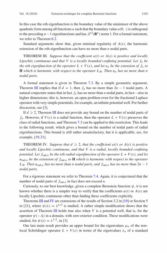
In this case the nth eigenfunction is the boundary value of the minimiser of the abovequadratic form among all functions u such that the boundary value u(0, ·) is orthogonalto the preceding n−1 eigenfunctions and hasL 2(Rn) norm 1. For a formal statement,we refer to Theorem 6.2.Standard arguments show that, given minimal regularity of A(s), the harmonic

extension of the nth eigenfunction can have no more than n nodal parts.

THEOREM III. Suppose that the coefficient a(t) or A(s) is positive and locallyLipschitz continuous and that V is a locally bounded confining potential. Let fn bethe nth eigenfunction of the operator L + V (x), and let un be the extension of fn toH which is harmonic with respect to the operator L H . Then un has no more than nnodal parts.

A formal statement is given in Theorem 7.3. By a simple geometric argument,Theorem III implies that if d = 1, then fn has no more than 2n − 1 nodal parts. Anatural conjecture states that in fact fn has no more than n nodal parts, in fact—also inhigher dimensions; this is, however, an open problem even for the fractional Laplaceoperator with very simple potentials, for example, an infinite potential well. For furtherdiscussion, see [3].

If d � 2, Theorem III does not provide any bound on the number of nodal parts offn . However, if V (x) is a radial function, then the operator L + V (x) preserves theclass of radial functions, and Theorem 7.3 can be applied to this restriction. This leadsto the following result, which gives a bound on the number of nodal parts of radialeigenfunctions. This bound is still rather unsatisfactory, but it is applicable; see, forexample, [19,21].

THEOREM IV. Suppose that d � 2, that the coefficient a(t) or A(s) is positiveand locally Lipschitz continuous, and that V is a radial, locally bounded confiningpotential. Let frad,n be the nth radial eigenfunction of the operator L + V (x), and leturad,n be the extension of frad,n to H which is harmonic with respect to the operatorL H . Then urad,n has no more than n nodal parts, and frad,n has no more than 2n − 1nodal parts.

For a rigorous statement we refer to Theorem 7.4. Again, it is conjectured that thenumber of nodal parts of frad,n in fact does not exceed n.Curiously, to our best knowledge, given a complete Bernstein function ψ , it is not

known whether there is a simpler way to verify that the coefficients a(t) or A(s) arelocally Lipschitz continuous other than finding these coefficients explicitly.Theorems III and IV are extensions of the results of Section 3.2 in [19] or Section 5

in [21], where ψ(λ) = λα/2 is studied. A rather simple modification shows that theassertion of Theorem III holds true also when V is a potential well, that is, for theoperator ψ(−�) in a domain, with zero exterior condition. These modifications werestudied, for ψ(λ) = λ1/2, in [3].Our last main result provides an upper bound for the eigenvalues μn of the non-

local Schrödinger operator L + V (x) in terms of the eigenvalues λn of a standard


Schrödinger operator −� + γ V (x) for an appropriate constant γ (depending on n).For simplicity, below we state the result for the fractional Laplace operator and ho-mogeneous potentials, which is identical to Corollary 8.2. For a more general version,we refer to Theorem 8.1.

THEOREM V. Suppose that V is a locally bounded, positive (except at zero)potential which is homogeneous with degree p > 0. Let λn be the eigenvalues of−� + V (x), and let μn be the eigenvalues of (−�)α/2 + V (x). Then

μn � ( 2α)α/(α+p)λ

(2+p)α/(2α+2p)n .

As p → ∞, the abovebound approximates thewell-knownboundμn � λα/2n for the

eigenvalues of (−�)α/2 and −� in a domain, with zero boundary/exterior condition.This was proved (for general complete Bernstein functions ψ) by DeBlassie [11] andChen and Song [9].

An estimate related to that of Theorem V was proved recently in [29]. Furtherresults on spectral theory of non-local Schrödinger operators can be found, amongothers, in [6,17,20,26,27,30–32,35,36,38,41,42].The structure of the article corresponds to the above description of main results.

We begin with a short section on preliminary results. Then we outline Krein’s spectraltheory of strings in Sect. 3; a more in-depth discussion is deferred to “Appendix A”.In Sect. 4 we introduce the harmonic extension technique and prove Theorems I andII. After that we discuss a number of examples in Sect. 5. Next three sections discussapplications to non-local Schrödinger operators: the variational principle (Sect. 6), theCourant–Hilbert theorem (Sect. 7) and estimates of eigenvalues (Sect. 8).We concludethe paper with a brief discussion on probabilistic aspects of the extension method.

2. Preliminaries

In this section we collect definitions and known results for later use. Throughout thetext d = 1, 2, . . . denotes the dimension. We typically use letters f, g, h for functionsdefined on Rd , and letters u, v, w for functions on the half-space H = (0,∞) × Rd .We denote the Lebesgue space of p-integrable functions on a domain D by L p(D).By F f we denote the isometric Fourier transform of a function f : if f ∈ L 1(Rd),then

F f (ξ) = (2π)−d/2∫Rd

e−iξ ·x f (x)dx,

and F extends to a unitary operator on L 2(Rd).

2.1. Complete Bernstein functions

Functions ψ : [0,∞) → [0,∞) of the form

ψ(λ) = c1 + c2λ + 1

π

∫(0,∞)

λ

λ + s

m(ds)

s


for some constants c1, c2 � 0 and some non-negative measurem that satisfies the inte-grability condition

∫(0,∞)

s−1(1+ s)−1m(ds) < ∞ are said to be complete Bernsteinfunctions. This class has found numerous applications in various areas ofmathematics,and it admits several characterisations, of which we mention two:

(1) A function ψ : [0,∞) → [0,∞) is a complete Bernstein function if and onlyif it extends to a holomorphic function of λ ∈ C\(−∞, 0], with Imψ(λ) � 0whenever Im λ � 0 (that is, ψ is a Pick function which is non-negative on(0,∞)).

(2) The class of complete Bernstein functions coincides with the class of non-negative operator monotone functions, that is, functions ψ such that ψ(L2) −ψ(L1) are non-negative definite whenever L1, L2 are self-adjoint operators suchthat L1 and L2 − L1 are non-negative definite.

Yet another characterisation, which is crucial for our needs, is given by Krein’s corre-spondence, as stated in Theorem 3.1. For a detailed discussion of complete Bernsteinfunctions we refer to [48].

2.2. Weak differentiability and ACL property

As usual, by ∂ j we denote the derivative along j th coordinate, by ∇ the gradient,and by � the Laplace operator. We use the same symbol ∂ j for pointwise and weakderivatives. Recall that a locally integrable function f defined on a domain D ⊆ Rd

is weakly differentiable if and only if there exist functions ∂ j f , j = 1, 2, . . . , d, suchthat

∫D

∂ j f (x)g(x)dx = −∫

Df (x)∂ j g(x)dx,

for all g ∈ C∞c (D) (infinitely smooth, compactly supported functions), where ∂ j g is

the usual derivative of g.

For brevity, by an absolutely continuous function we will always mean a locallyabsolutely continuous function. In dimension one, f is weakly differentiable if andonly if it is equal almost everywhere to an absolutely continuous function f . In thiscase f is differentiable almost everywhere, f (y) − f (x) is equal to the integral of f ′over [x, y], and the weak derivative of f is equal (almost everywhere) to f ′.

A similar description is available in higher dimensions, using absolute continuityon lines, abbreviated as ACL. Namely, a function f has the ACL property if, for everycardinal direction, f is absolutely continuous on almost every line in that direction.A well-known theorem asserts that f is weakly differentiable if and only if it is equalalmost everywhere to a function f with the ACL property such that ∇ f (x) is locallyintegrable in D.


3. Krein’s spectral theory of strings

3.1. Fundamental result

The harmonic extension technique is based onKrein’s spectral theory of strings. Ourstarting point is the following theorem, which is essentially due to Krein. Referencesand further discussion can be found in “Appendix A”.

THEOREM 3.1. Suppose that A(s) is a non-negative locally integrable functionon [0,∞). Then for every λ � 0 there exists a unique non-increasing function ϕλ(s)on [0,∞) which solves

⎧⎪⎪⎨⎪⎪⎩

ϕ′′λ(s) = λA(s)ϕλ(s) for s > 0,

ϕλ(0) = 1,

lims→∞ ϕλ(s) � 0

(3.1)

(with the second derivative understood in the weak sense). Furthermore, the expression

ψ(λ) = −ϕ′λ(0)

defines a complete Bernstein function ψ , and the correspondence between A(s) andψ(λ) is one-to-one.

More generally, let A be a Krein’s string: a locally finite non-negative Borel mea-sure A(ds) on [0, R), where R ∈ (0,∞]. Then for every λ � 0 there is a uniquenon-increasing function ϕλ(s) on [0, R) which solves problem (3.1) (with the sec-ond derivative understood in the sense of distributions), with an additional Dirichletboundary condition ϕλ(R) = 0 at s = R imposed in the case when R is finite and(R − s)A(ds) is a finite measure.

Furthermore, any nonzero complete Bernstein function ψ can be obtained in theabove manner in a unique way.

We remark that the Neumann boundary condition ϕ′λ(R) = 0 would correspond to

extending the string to [0,∞) in such a way that A = 0 on [R,∞). If (R − s)A(ds)is an infinite measure on a finite interval [0, R), then the Dirichlet condition at s = Ris automatically satisfied.We also note that when R = ∞ or when (R − s)A(ds) is an infinite measure on

a finite interval [0, R), then any solution of the first equation in (3.1) which is not amultiple of ϕλ necessarily diverges to ∞ or −∞ as s → ∞.In order not to overwhelm the reader with technical details, throughout the article

we restrict our attention to the regular case, that is, we will assume that A is a non-negative locally integrable function on [0,∞). The extension to the general case isdiscussed in “Appendix A”, where also the existence and properties of ϕλ are furtherdiscussed. More information about Krein’s spectral theory of strings can be found, forexample, in Chapter 5 of [15], in [34] and in Chapter 15 of [48].


Note that ϕλ is non-increasing and convex, so that in particular

0 � −ϕ′λ(s) � ϕλ(0) − ϕλ(s)

s� 1

s(3.2)

for all s > 0 and λ � 0. Although this estimate is very rough, it is completely sufficientfor our needs.Wewill need the following rather standard property: if f is an absolutely continuous

function satisfying f (0) = 1, then∫ ∞

0

(( f ′(s))2 + λA(s)( f (s))2

)ds � ψ(λ), (3.3)

and equality holds if and only if f = ϕλ. For completeness, we provide a short proof.Equality for f = ϕλ follows by integration by parts: we have ϕλ(0)ϕ′

λ(0) = −ψ(λ),and ϕλ(s)ϕ′

λ(s) converges to zero as s → ∞, so that

∫ ∞

0(ϕ′

λ(s))2ds = ψ(λ) −

∫ ∞

0ϕλ(s)ϕ

′′λ(s)ds.

Since ϕ′′λ(s) = λA(s)ϕλ(s), equality in (3.3) for f = ϕλ follows.

Suppose now that f is absolutely continuous and f (0) = 1. Estimate (3.3) holdstrivially if f ′ is not square integrable. Otherwise, by Schwartz inequality, for S > 0we have

| f (S) − f (0)|2 �(∫ S

0| f ′(s)|ds

)2

� S∫ S

0| f ′(s)|2ds � S

∫ ∞

0| f ′(s)|2ds.

(3.4)

Therefore, | f (S)| � 1 + (S∫ ∞0 | f ′(s)|2ds)1/2 for all S > 0. In particular, by (3.2),

f (s)ϕ′λ(s) converges to zero as s → ∞. Denote g(s) = f (s) − ϕλ(s). Then g is an

absolutely continuous function, g(0) = 0 and g(s)ϕ′λ(s) converges to zero as s → ∞.

Therefore, integration by parts gives∫ ∞

0g′(s)ϕ′

λ(s)ds = −∫ ∞

0g(s)ϕ′′

λ(s)ds = −∫ ∞

0λA(s)g(s)ϕλ(s)ds.

Clearly,∫ ∞

0

(( f ′(s))2 + λA(s)( f (s))2

)ds =

∫ ∞

0

((ϕ′

λ(s))2 + λA(s)(ϕλ(s))

2)ds

+ 2∫ ∞

0

(ϕ′

λ(s)g′(s) + λA(s)ϕλ(s)g(s)

)ds

+∫ ∞

0

((g′(s))2 + λA(s)(g(s))2

)ds.

We already know that the first integral in the right-hand side is equal to ψ(λ), whilethe middle one is zero. The last one is non-negative, and it is equal to zero if and only


if g′(s) = 0 for almost all s, which implies that g is identically zero. The proof of (3.3)is complete.We record that for λ > 0,

∫ ∞

0A(s)(ϕλ(s))

2ds = ψ ′(λ). (3.5)

This identity is used only in the last section, where the estimates of eigenvalues ofSchrödinger operators are studied. In order to prove (3.5), observe that integrating byparts as in the proof of equality in (3.3), we obtain

∫ ∞

0ϕ′

μ(s)ϕ′λ(s)ds = ψ(λ) −

∫ ∞

0ϕμ(s)ϕ′′

λ(s)ds,

that is,

ψ(λ) =∫ ∞

0

(ϕ′

μ(s)ϕ′λ(s) + λA(s)ϕμ(s)ϕλ(s)

)ds

forμ, λ > 0. Combining the above identitywith a similar one, obtained by exchangingthe roles of μ and λ, we find that

ψ(μ) − ψ(λ) = (μ − λ)

∫ ∞

0A(s)ϕμ(s)ϕλ(s)ds.

We divide both sides by μ − λ and pass to the limit as λ → μ. Observe thatϕμ(s)ϕλ(s) � (ϕλ/2(s))2 whenμ > λ/2, and A(s)(ϕλ/2(s))2 is integrable by equalityin (3.3). Therefore, by dominated convergence

ψ ′(λ) =∫ ∞

0A(s)

(limμ→λ

ϕμ(s)

)ϕλ(s)ds.

To complete the proof of (3.5), it remains to observe that ϕμ(s) depends continuouslyon μ (see “Appendix A.3” for further details).

3.2. Change of variable

Suppose that a(t) is a Borel function on (0,∞), with values in [0,∞], such thatσ(T ) = ∫ T

0 (a(t))−1dt is strictly increasing and finite for all T > 0, and such thatσ(t) diverges to infinity as t → ∞. Then A(σ (t)) = (a(t))2 defines a Borel functionA(s) on (0,∞).Conversely, if a positive, Borel function A(s) is given, then the corresponding

σ(t) and a(t) = 1/σ ′(t) can be found by solving the ordinary differential equationA(σ (t)) = (σ ′(t))−2, that is, they are described by the identity

∫ σ(t)

0

√A(s) ds = t


for t ∈ (0,∞). In order that σ(t) is indeed well defined and continuous, we needto assume that the integral of (A(s))1/2 is strictly increasing, finite and divergentto infinity as s → ∞; for absolute continuity of σ (required for the definition ofa(t) = (σ ′(t))−1), additional conditions on A(s) need to be imposed.

After a change of variable s = σ(t), we find that∫A(s)ds =

∫A(σ (t))σ ′(t)dt =

∫a(t)dt.

Therefore, local integrability of a(t) on [0,∞) is equivalent to local integrability ofA(s) on [0,∞).Suppose that f (t) = f (σ (t)). Note that σ(t) is absolutely continuous and mono-

tone. It follows that if f is absolutely continuous, then so is f . The converse is alsotrue, since the inverse function σ−1(s) is absolutely continuous (as a consequence ofthe fact that σ ′(t) = (a(t))−1 is positive almost everywhere due to local integrabilityof a(t)). The derivatives (either pointwise or weak) of f and f are related by theidentity

a(t) f ′(t) = a(t) f ′(σ (t))σ ′(t) = f ′(σ (t))

for almost all t .If f ′ is absolutely continuous, then it follows that a(t) f ′(t) is absolutely continuous,

and furthermore,

(a(t))−1(a(t) f ′(t))′ = (a(t))−1 f ′′(σ (t))σ ′(t)= (a(t))−2 f ′′(σ (t)) = (A(σ (t)))−1 f ′′(σ (t)). (3.6)

In otherwords, the operator (a(t))−1∂t (a(t)∂t ) is equivalent to theoperator (A(s))−1∂2safter a change of variable s = σ(t). This explains the identification of Dirichlet-to-Neumann operators given by (1.6) and (1.8) on the one hand, and by (1.5) and (1.7)on the other.We will need a similar correspondence in terms of quadratic forms. If f (σ (t)) =

f (t), we clearly have∫ ∞

0a(t)( f (t))2dt =

∫ ∞

0(a(t))2( f (σ (t)))2σ ′(t)dt =

∫ ∞

0A(s)( f (s))2ds. (3.7)

Furthermore, if f or f is weakly differentiable, then∫ ∞

0a(t)( f ′(t))2dt =

∫ ∞

0(a(t))−1 f ′(σ (t)))2dt =

∫ ∞

0( f ′(s))2ds. (3.8)

4. Extension technique

4.1. Quadratic form in half-space

Throughout the entire section we assume that A(s) is a non-negative, locally inte-grable function on [0,∞). Recall that H = (0,∞) × Rd .


DEFINITION 4.1. For a function u on H, we define

EH (u, u) =∫ ∞

0

∫Rd

((∂su(s, x))2 + A(s)|∇x u(s, x)|2

)dxds. (4.1)

The domain of this form, denoted D(EH ), is the set of all locally integrable functionsu on H which satisfy the following conditions: u(s, x) is weakly differentiable withrespect to s, (A(s))1/2u(s, x) is weakly differentiable with respect to x , the integralin (4.1) is finite, and ∫ s1

s0

∫Rd

A(s)|u(s, x)|2dxds < ∞ (4.2)

whenever 0 < s0 < s1.

Note that if A(s) is locally bounded below by a positive constant, then we can sim-ply say that u(s, x) is weakly differentiable with respect to both s and x . However, forgeneral A, the function (A(s))−1/2 may fail to be integrable, and therefore weak differ-entiability of (A(s))1/2u(s, x) with respect to x need not imply weak differentiabilityof u(s, x) with respect to x . In this case, the second term under the integral in (4.1)should in fact be understood as |∇x ((A(s))1/2u(s, x))|2; for simplicity, however, weabuse the notation and we use the less formal expression A(s)|∇x u(s, x)|2.

The quadratic form EH is closed in the following sense: if un ∈ D(EH ) is a funda-mental sequence with respect to the semi-norm (EH (·, ·))1/2 which converges in thenorm ofL 2((s0, s1) ×Rd) (for any s0, s1 such that 0 < s0 < s1) to some function u,then u ∈ D(EH ) and un converges to u in the semi-norm (EH (·, ·))1/2. This followsby a standard argument; see “Appendix A.1” for details. We remark that if u is afunction harmonic for operator (1.6), then typically u does not belong toL 2(H), butthe expression in (4.1) is finite. For this reason, we define the form EH on a domainwhich is not contained in L 2(H). However, if EH is restricted to D(EH ) ∩ L2(H),then it becomes a Dirichlet form: it is symmetric, non-negative, Markovian, denselydefined and closed.The definition of the domain of EH resembles in some sense the definition of the

weighted Sobolev space W 1,2(H, A(s)dsdx). However, the coefficient A is allowedto be highly singular: it can be equal to zero on large sets and can have arbitrary(integrable) singularities, and in “Appendix A” we even allow A to be an arbitrarylocally finite measure. Therefore, the space D(EH ) does not appear to be related toany of the standard function spaces studied in the literature.Clearly, EH defined above is the quadratic form of the operator

L H u(s, x) = ∂2s u(s, x) + A(s)�x u(s, x).

As this operator will only be used in the weak sense, we do not need to specify thedomain of L H .LetFx u(s, ·) denote the Fourier transform of u(s, ·). By Plancherel’s theorem, one

easily finds that u ∈ D(EH ) if and only if Fx u(s, ξ) is weakly differentiable withrespect to s,


∫ s1

s0

∫Rd

A(s)|Fx u(s, ξ)|2dxds < ∞ (4.3)

whenever 0 < s0 < s1, and the integral in the right-hand side of the identity

EH (u, u) =∫ ∞

0

∫Rd

(|∂sFx u(s, ξ)|2 + A(s)|ξ |2|Fx u(s, ξ)|2

)dξds (4.4)

is finite; the above equality expresses EH in terms of the Fourier transform.If u ∈ D(EH ), then ∂su(s, ·), as an L 2(Rd)-valued function, is locally integrable

on [0,∞) (in the sense of Bochner’s integral). Indeed, by Schwarz inequality,

(∫ s1

s0‖∂su(s, ·)‖2ds

)2

� (s1 − s0)∫ s1

s0‖∂su(s, ·)‖22ds � (s1 − s0)EH (u, u)

(4.5)

whenever 0 � s0 < s1. (This is an analogue of (3.4).) Furthermore, one easily seesthat for almost all S, the Bochner integral

∫ S

0∂su(s, ·)ds

is equal to u(S, ·) − u0(·) for some function (“constant”) u0 ∈ L 2(Rd). If we denoteu(0, ·) = u0(·), then, after modification on a set of zero Lebesgue measure, we mayassume that in fact

u(S, ·) = u(0, ·) +∫ S

0∂su(s, ·)ds, (4.6)

for all S ∈ [0,∞). Observe that (4.6) and (4.5) imply that

‖u(s, ·)‖2 � ‖u(0, ·)‖2 + (sEH (u, u))1/2. (4.7)

From now on we will always assume that (4.6) holds for all S ∈ [0,∞) whenever weconsider u ∈ D(EH ).

4.2. Boundary form

The trace E ( f, f ) of the quadratic form EH (u, u) on the boundary of H is definedas the minimal value of EH (u, u) among all u ∈ D(EH ) which satisfy the boundarycondition u(0, x) = f (x). It is not very difficult to see that the minimisers u areharmonic functions with respect to L H , and these harmonic functions can be describedin terms of the Fourier transform and the functions ϕλ introduced in Sect. 3. A shortcalculation reveals that in fact

E ( f, f ) =∫Rd

ψ(|ξ |2)| f (ξ)|2dξ, (4.8)

where ψ(λ) = −ϕ′λ(0) is a complete Bernstein function described by Theorem 3.1.


We take (4.8) as the definition, with the domainD(E ) defined to be the space of allf ∈ L 2(Rd) for which the integral in definition (4.8) of E ( f, f ) is finite. With thisdefinition, we will prove that indeed E ( f, f ) is the trace of EH (u, u) on the boundary.We also denote by L = ψ(−�) the Fourier multiplier with symbol ψ(|ξ |2), that is,as in (1.3),

F (L f )(ξ) = ψ(|ξ |2)F f (ξ),

with domain D(L) consisting of those f ∈ L 2(Rd) for which ψ(|ξ |2)F f (ξ) issquare integrable.Let ϕ(λ, s) = ϕλ(s) be the function defined in Theorem 3.1. We introduce the

harmonic extension operator.

DEFINITION 4.2. For f ∈ L 2(Rd) we define its harmonic extension u = ext( f )

to H by means of Fourier transform,

Fx u(s, ξ) = ϕ(|ξ |2, s)F f (ξ),

where Fx u(s, ·) is the Fourier transform of u(s, ·).Since ϕ(λ, s) is bounded by 1, the harmonic extension is well defined and we have

‖u(s, ·)‖2 � ‖ f ‖2. We begin by observing that the Dirichlet-to-Neumann operatorapplied to ext( f ) coincides with L f .

THEOREM 4.3. Let f ∈ L 2(Rd) and u = ext( f ). Then f ∈ D(L) if and only ifthe limit in the definition of ∂su(0, ·) exists in L 2(Rd), and in this case

L f = −∂su(0, ·) = − lims→0+ ∂su(s, ·).

Proof. Recall that −∂sϕ(λ, s) is decreasing and equal to ψ(λ) for s = 0. Thus,if f ∈ D(L), then the desired result follows by dominated convergence. On theother hand, if the limit in the definition of ∂su(0, ·) exists, then ψ(ξ2) f (ξ) is squareintegrable by monotone convergence, and so f ∈ D(L). �

Our next two results state that E ( f, f ) = EH (u, u) if u = ext( f ) and that ext( f )

indeed minimises E (u, u) among all u ∈ D(EH ) such that u(0, x) = f (x).

THEOREM 4.4. Let f ∈ L 2(Rd) and u = ext( f ). Then u ∈ D(EH ) if and onlyif f ∈ D(E ), and in this case

E ( f, f ) = EH (u, u).

Proof. Since ‖u(s, ·)‖2 � ‖ f ‖2 and since A(s) is locally integrable,

∫ s1

s0

∫Rd

A(s)|u(s, x)|2dxds < ∞


whenever 0 < s0 < s1. By equality in (3.3) and Fubini,∫ ∞

0

∫Rd

(|∂sFx u(s, ξ)|2 + A(s)|ξ |2|Fx u(s, ξ)|2

)dξds

=∫ ∞

0

∫Rd

((∂sϕ(|ξ |2, s))2 + A(s)|ξ |2(ϕ(|ξ |2, s))2

)|F f (ξ)|2dξds

=∫Rd

ψ(|ξ |2)|F f (ξ)|2dξ.

(4.9)

If u ∈ D(EH ), then the left-hand side is equal to EH (u, u) (by (4.4)), and therefore,f ∈ D(E ) and E ( f, f ) = EH (u, u). Conversely, if f ∈ D(E ), then the right-handside of the equality (4.9) is finite. Therefore, Fx u(s, ξ) is weakly differentiable withrespect to s and the expression in (4.4) is finite. We conclude that u ∈ D(EH ), asdesired. �

THEOREM4.5. Let v ∈ D(EH ), f (x) = v(0, x) and u = ext( f ). Then f ∈ D(E )

and

EH (v, v) � EH (u, u) = E ( f, f ).

Moreover, the space D(EH ) is a direct sum of D0 and Dharm, where

D0 = {u ∈ D(EH ) : u(0, x) = 0 for almost all x ∈ Rd},Dharm = {ext( f ) : f ∈ D(E )}

are orthogonal to each other with respect to EH .

Proof. Let v ∈ D(EH ) and f (x) = v(0, x). By (4.4),

EH (v, v) =∫ ∞

0

∫Rd

(|∂sFxv(s, ξ)|2 + A(s)|ξ |2|Fxv(s, ξ)|2

)dξds.

By the ACL characterisation, after modification on a set of zero Lebesgue measure,for almost all ξ ∈ Rd , the functionFxv(·, ξ) is absolutely continuous on [0,∞), andthe pointwise and weak definitions of ∂sFxv(s, ξ) coincide for almost all s. Denotethis modification by w(s, ξ). For those ξ for which w(·, ξ) is absolutely continuous,w(0, ξ) = 0 and w(·, ξ) is square integrable on (0,∞), we have, by (3.3),

∫ ∞

0

(|∂sw(s, ξ)|2 + A(s)|ξ |2|w(s, ξ)|2

)ds � ψ(|ξ |2)|w(0, ξ)|2.

(We applied (3.3) to f (s) = Re(w(s, ξ)/w(0, ξ)) and λ = |ξ |2.) The above inequalityis also trivially true when w(0, ξ) = 0. These two cases cover almost all ξ ∈ Rd .Therefore, by Fubini,

EH (v, v) �∫Rd

ψ(|ξ |2)|w(0, ξ)|2dξ.


Observe that w(s, ξ) converges to w(0, ξ) as s → 0+ for almost all ξ ∈ Rd . Onthe other hand, by (4.7) we know that v(s, ·) converges to f in L 2(Rd). However,w(s, ·) = Fxv(s, ·) for almost all s, and so a subsequence ofw(s, ·) converges toF fin L 2(Rd). Therefore, w(0, ξ) = F f (ξ) for almost all ξ ∈ Rd , and we concludethat f ∈ D(E ) and

EH (v, v) � E ( f, f ).

The first part of the theorem follows now by Theorem 4.4. Furthermore, if we denoteu = ext( f ), then u ∈ Dharm and v − u ∈ D0, so that indeedD(EH ) is a sum ofDharm

and D0.Orthogonality of Dharm and D0 follows now by a standard argument: if u ∈ Dharm,

v ∈ D0 and α ∈ R, then EH (u + αv, u + αv) � EH (u, u), which reduces to

2αEH (u, v) + α2EH (v, v) � 0;

thus, EH (u, v) = 0. (Here, of course, EH (u, v) denotes the Hermitian form corre-sponding to the quadratic form EH (u, u).) �

We conclude this section with a result that explains the name harmonic extensionused for the function ext( f ).

THEOREM4.6. If f ∈ L 2(Rd), then the harmonic extension u = ext( f ) satisfies

∂2s u(s, x) + A(s)�x u(s, x) = 0 (4.10)

in H in the weak sense. Conversely, if u satisfies (4.10) in H in the weak sense and‖u(s, ·)‖2 is a bounded function of s, then u = ext( f ) for some f ∈ L 2(Rd).

Proof. We understand (4.10) as

∫ ∞

0

∫Rd

u(s, x)(∂2s v(s, x) + A(s)�xv(s, x))dxds = 0 (4.11)

for all test functions v ∈ C∞c (H). If u = ext( f ), then, by Plancherel’s theorem, the

left-hand side of (4.11) is equal to

∫ ∞

0

∫Rd

F f (ξ)ϕ(|ξ |2, s)(∂2s Fxv(s, ξ) − A(s)|ξ |2Fxv(s, ξ))dξds.

For any ξ ∈ Rd the integral over s ∈ (0,∞) is zero due to the fact that ϕ′′λ(s) =

−λA(s)ϕλ(s) in the weak sense. The first statement is thus proved.To prove the second one, we use a similar argument: Plancherel’s theorem implies

that for any g ∈ C∞c ((0,∞)) and h ∈ C∞

c (Rd),

∫ ∞

0

∫Rd

Fx u(s, ξ)(g′′(s) − A(s)g(s)|ξ |2)Fh(ξ)dξds = 0.


By considering a countable and linearly dense set of pairs g ∈ C∞c ((0,∞)) and

h ∈ C∞c (Rd), we see that for almost all ξ ∈ Rd , Fx u(·, ξ) is a weak solution of

ϕ′′(s) = |ξ |2A(s)ϕ(s). Such a solution is either a multiple of ϕ(|ξ |2, s), or a functionthat diverges to ±∞ as s → ∞. Since the L 2(Rd) norms of Fx u(s, ·) are boundedas s → ∞, for almost all ξ ∈ Rd we have Fx u(s, ξ) = ϕ(|ξ |2, s)F(ξ) for someF(ξ). Using again boundedness of ‖Fx u(s, ·)‖2 we conclude that F ∈ L 2(Rd), andtherefore, u = ext(F−1F). �

4.3. Change of variable

We now rephrase the results of the previous section in terms of operator (1.5).Suppose that a(t) is a locally integrable non-negative function on [0,∞) such that(a(t))−1 is also locally integrable, but not integrable, on [0,∞). An extension to thecase when (a(t))−1 is integrable on [0,∞) is discussed in “Appendix A.2”.

Following Sect. 3.2, we define

σ(T ) =∫ T

0(a(t))−1dt.

Using the results of Sect. 3.2, we can identify the quadratic form EH defined earlierin this section with the following one.

DEFINITION 4.7. For a function u on H, the quadratic form EH (u, u) is definedby the expression

EH (u, u) =∫ ∞

0

∫Rd

a(t)|∇t,x u(t, x)|2dxdt. (4.12)

The domain D(EH ) of this form is the set of all locally integrable functions u on Hwhich satisfy the following conditions: u(t, x) is weakly differentiable with respectto t , (a(t))1/2u(t, x) is weakly differentiable with respect to x , the integral in (4.12)is finite, and ∫ t1

t0

∫Rd

a(t)|u(t, x)|2dxdt < ∞ (4.13)

whenever 0 < t0 < t1. Finally, if f ∈ L 2(Rd), then we define its harmonic extensionu = ext f by u(t, x) = u(σ (t), x), where u = ext( f ).

The domain of EH is very similar to theweighted Sobolev spaceW 1,2(H, a(t)dtdx);in the definition ofD(EH ), however,wedonot require that the integral ofa(t)(u(t, x))2

overH is finite. Nevertheless, the coefficient a(t) can be very rough, so standard theoryof weighted Sobolev spaces seems to be of little use for our needs.Recall that under our assumptions, the function A(s) defined by A(σ (t)) = (a(t))2

is locally integrable on [0,∞). Equivalence of the quadratic forms EH and EH , aswell as the corresponding Dirichlet-to-Neumann operators, is very simple when thecoefficients are regular enough. In the general case, one needs to pay extra attentionto domains.


LEMMA 4.8. Suppose that u(σ (t), x) = u(t, x). Then u ∈ D(EH ) if and only ifu ∈ D(EH ), and in this case EH (u, u) = EH (u, u).

Proof. Recall that if f (σ (t)) = f (t), then absolute continuity of f (s) is equivalentto absolute continuity of f (t). By the ACL characterisation of weak differentiability,weak differentiability of u(s, x)with respect to s is equivalent to weak differentiabilityof u(t, x) with respect to t .

Using the same method together with formula (3.7), we see that weak differentia-bility of (A(s))1/2u(s, x) with respect to x is equivalent to weak differentiability of(a(t))1/2u(t, x) with respect to x .By (3.7) and (3.8), the integrals definingEH (u, u) and EH (u, u) are equal. Similarly,

by (3.7), the integrals in (4.2) and (4.13) are equal if s0 = σ(t0) and s1 = σ(t1).Therefore, u ∈ D(EH ) if and only if u ∈ D(EH ), and we already noted that in thiscase EH (u, u) = EH (u, u). �

The following result follows almost immediately from Theorems 4.3 and 4.6.

THEOREM 4.9. Suppose that f ∈ L 2(Rd) and u = ext( f ). Then u satisfies

∂t,x (a(t)∂t,x u(t, x)) = 0 (4.14)

in H in the weak sense. Furthermore, f ∈ D(L) if and only if any of the limits in theidentity

L f = − limt→0+

u(t, ·) − u(0, ·)σ (t)

= − limt→0+ a(t)∂t u(t, ·)

exists in L 2(Rd). Finally, if u satisfies (4.14) in the weak sense and ‖u(t, ·)‖2 is abounded function of t , then u = ext( f ) for some f ∈ L 2(Rd).

Proof. The first and the last statements are merely a reformulation of Theorem 4.6,combinedwith identification (3.6) of the operators (A(s))−1∂2s and (a(t))−1∂t (a(t)∂t ):for any test function v ∈ C∞

c (H) and v(t, x) = v(σ (t), x) we have

∫ ∞

0

∫Rd

∇t,x (a(t)∇t,x u(t, x))v(t, x)dxdt

=∫ ∞

0

∫Rd

u(t, x)∇t,x (a(t)∇t,x v(t, x))dxdt

=∫ ∞

0

∫Rd

a(t)u(t, x)((a(t))−1∂t (a(t)∂t v(t, x)) + �x v(t, x))dxdt

=∫ ∞

0

∫Rd

A(s)u(s, x)((A(s))−1∂2s v(s, x) + �xv(s, x))dxds

=∫ ∞

0

∫Rd

(∂2s u(s, x) + A(s)�x u(s, x))v(s, x)dxds.

The middle statement is a direct consequence of Theorem 4.3. �


By combining Lemma 4.8 with Theorems 4.4 and 4.5, we immediately get thefollowing result.

THEOREM 4.10. Let f ∈ L 2(Rd) and u = ext( f ). Then f ∈ D(E ) if and onlyif u ∈ D(EH ). If v ∈ D(EH ), f (x) = v(0, x) and u = ext( f ), then f ∈ D(E ) and

EH (v, v) � EH (u, u) = E ( f, f ).




5. Examples

Before we proceed with applications of the extension technique introduced in theprevious section, we discuss several examples. Noteworthy, there is only a handfulof known pairs of explicit coefficients A(s) (or a(t)) and corresponding completeBernstein functions ψ(λ); Chapter 15 in [48] contains a concise table in a different(probabilistic) language. This is, however, not an essential problem in most applica-tions of the variational principles of Theorem 6.2, because in order to use them, onetypically does not require an explicit form of the coefficients: it is sufficient to knowthat appropriate coefficients A(s) or a(t) exist.

Throughout this section, as it is the case in Introduction, we drop tilde from thenotation, and write u(t, x) for what was denoted by u(t, x) in Sect. 4.3. We alsosimply write ϕλ(t) instead of more formal ϕλ(σ (t)).Most examples below are arranged in the following way: we begin with coefficients

A(s) or a(t) and find the corresponding ϕλ(s) or ϕλ(t). The harmonic extensionu = ext( f ) for operator (1.5) is then given by

Fx u(t, ξ) = ϕλ(t)F f (ξ),

where λ = |ξ |2.5.1. Classical Dirichlet-to-Neumann operator

Let A(s) = 1, or a(t) = 1. Then σ(t) = t , so the two parametrisations areidentical. Clearly, ϕλ(t) = exp(−λ1/2t), ψ(λ) = λ1/2, and we recover the classicalresult: if u(t, x) is harmonic in H (that is, �t,x u(t, x) = 0 in H) with boundary valueu(0, x) = f (x), then∫

Rd|ξ ||F f (ξ)|2dξ =

∫ ∞

0

∫Rd

|∇t,x u(t, x)|2dxdt,

(−�)1/2 f = ∂t u(0, ·). (5.1)


Two things need to be clarified here. In this section we understand that in expressionssimilar to (5.1) one side is defined (i.e. the integral is finite in either side of the firstequality; |ξ |F f (ξ) is square integrable in the left-hand side of the second equality;the partial derivative exists with a limit in L 2(Rd) in the right-hand side of thesecond equality) if and only if the other one is also defined. Furthermore, we need toimpose some boundedness condition to assert that indeed u = ext( f ) in the sense ofDefinition 4.2. By Theorem 4.6, it is sufficient to assume that u is twice differentiablein the weak sense, with u(s, ·) bounded in L 2 for s ∈ (0,∞), and that harmonicityis understood in the weak sense. Note, however, that in most cases this condition canbe significantly relaxed.

5.2. Caffarelli–Silvestre extension technique

Let α ∈ (0, 2), and define two constants:

cα = 2α�(α/2)|�(−α/2)|−1, Cα = 21−α/2(�(α/2))−1.

Consider the coefficients

A(s) = α−2c2/αα s2/α−2 or a(t) = α−1cαt1−α.

Then one finds that

ϕλ(s) = Cα(cαλα/2s)1/2Kα/2((cαλα/2s)1/α),

ψ(λ) = λα/2,

where Kα/2 is the modified Bessel function of the second kind. In variable t , we have

σ(t) = c−1α tα,

ϕλ(t) = Cα(λ1/2t)α/2Kα/2(λ1/2t),

ψ(λ) = λα/2,

Therefore, if u(t, x) satisfies

∇t,x (t1−α∇t,x u(t, x)) = 0

in H with boundary value u(0, x) = f (x), then∫Rd

|ξ |α|F f (ξ)|2dξ =∫ ∞

0

∫Rd

α−1cαt1−α|∇t,x u(s, x)|2dxds

and

(−�)α/2 f = −α−1cα limt→0+ t1−α∂t u(t, ·).

This can be rewritten in variable s: if u(s, x) satisfies

∂2s u(s, x) + α−2c2/αα s2/α−2�x u(s, x) = 0


in H with boundary value u(0, x) = f (x), then∫Rd

|ξ |α|F f (ξ)|2dξ =∫ ∞

0

∫Rd

((∂su(s, x))2 + α−2c2/αα s2−2/α∇x u(s, x)|2

)dxds

and

(−�)α/2 f = −∂su(0, ·).This example was first studied by Molchanov and Ostrovski [44] in the language ofstochastic processes and then recently by Caffarelli and Silvestre [5] in the context ofnon-local partial differential equations; see Introduction for further references.

5.3. Quasi-relativistic operator

Let m > 0, and define

A(s) = (1 + 2ms)−2 or a(t) = e−2mt .

Then

ϕλ(s) = (1 + 2ms)(2m)−1(m−(m2+λ)1/2),

ψ(λ) = (m2 + λ)1/2 − m.

In variable t , we have

σ(t) = (2m)−1(e2mt − 1),

ϕλ(t) = e(m−(m2+λ)1/2)t .

Therefore, the quasi-relativistic operator (−� + m2)1/2 − m can be expressed as theDirichlet-to-Neumann operator for differential operators

∂2s u(s, x) + (1 + 2ms)−2�x u(s, x)

or

∇t,x (e−2mt∇t,x u(t, x))

in H. This example was studied, in the probabilistic context, in [45].

5.4. A string of finite length

A closely related example is obtained by considering

A(s) = (1 − 2ms)−2 or a(t) = e2mt ,

where in this case the range of s is finite: s ∈ (0, (2m)−1). The corresponding versionof the results of Sect. 4 is discussed in “Appendix A.2”.


Note that ((2m)−1−s)A(s) is not integrable, so thatϕλ(s) automatically satisfies theDirichlet condition at s = (2m)−1. In particular, A(s) is not integrable, and therefore,u(s, ·) automatically converges in L 2(Rd) to zero as s → ((2m)−1)− for everyu ∈ D(EH ). We have

ϕλ(s) = (1 − 2ms)(2m)−1(m+(m2+λ)1/2),

ψ(λ) = (m2 + λ)1/2 + m,

and in variable t ,

σ(t) = (2m)−1(1 − e−2mt ),

ϕλ(t) = e−(m+(m2+λ)1/2)t .

This gives a harmonic extension problem for the operator (−� + m2)1/2 + m, whichdiffers by a constant from the quasi-relativistic operator from the previous example.Since (λ + m2)1/2 is complete Bernstein function, there must be a corresponding

coefficient A(s) or a(t). To our knowledge, the explicit form for this coefficient is notknown. There is, however, a different way to represent (−� + m2)1/2: consider theclassical extension problem for−�+m2 instead of−�. This approach was exploitedin, for example, [1,4].

5.5. Quasi-relativistic-type operators

More generally, if ψ(−�) is the Dirichlet-to-Neumann operator for the differentialoperator (1.5), then it is easy to construct an analogous representation forψ(μ−�)−ψ(μ), where μ > 0. Indeed, denote

La f (t) = (a(t))−1(a(t) f ′(t))′ = f ′′(t) + (a(t))−1a′(t) f ′(t)

and observe that

La(ϕμ f ) = ϕμLa f + 2ϕ′μ f ′ + f Laϕμ

= ϕμLa f + 2ϕ′μ f ′ + μ f ϕμ.

On the other hand, if b(t) = a(t)(ϕμ(t))2, then

Lb f (t) = f ′′(t) + (a(t))−1a′(t) + 2(ϕμ(t))−1ϕ′μ(t) f ′(t).

Therefore,

ϕ−1μ La(ϕμ f ) = Lb f + μ f.

Set fλ(t) = (ϕμ(t))−1ϕμ+λ(t). Then

Lb fλ = ϕ−1μ La(ϕμ fλ) − μ fλ = ϕ−1

μ Laϕλ − μ fλ = (μ + λ)ϕ−1μ ϕλ − μ fλ = λ fλ.


Furthermore,

limt→0+ b(t) f ′

λ(t) = limt→0+ a(t)(ϕμ(t))2((ϕμ(t))−1ϕμ+λ(t))

′

= limt→0+ a(t)(ϕ′

μ+λ(t)ϕμ(t) − ϕμ+λ(t)ϕ′μ(t)) = ψ(μ + λ) − ψ(μ).

We conclude that the coefficient b(t) indeed corresponds to ψ(μ + λ) − ψ(μ).In particular, the operator (m2 − �)α/2 − mα is the Dirichlet-to-Neumann operator

for the differential operator

α−1cαmα∇t,x (t (Kα/2(mt))2∇t,x u(t, x));

here, we set μ = m2. This calculation is due to [13] in a probabilistic context.Note that the argument used in this section works well in variable t , but it is not

easy to reproduce in variable s: the operator (A(s))−1(ϕμ(s) f (s))′′ is not of the form(B(s))−1 f (s) + μ f (s) unless another change of variable is introduced.

5.6. Operators in the theory of linear water waves

In the theory of linear water waves, one often considers the Dirichlet-to-Neumannoperator for A(s) = 1, or a(t) = 1, in a finite interval (0, R) (which represents thedepth of the ocean). Since σ(t) = t , the two parametrisations coincide. A version ofthe results of Sect. 4 adapted to the present setting is discussed in “Appendix A.2”.Imposing Neumann boundary condition at t = R is equivalent to setting A(s) = 0

for s � R, and one easily finds that

ϕλ(t) = cosh(λ1/2(R − t))

cosh(λ1/2R),

ψ(λ) = λ1/2 tanh(λ1/2R).

The corresponding operator has Fourier symbol |ξ | tanh(R|ξ |).Dirichlet condition at t = R is equivalent to considering a string of finite length R,

and we get

ϕλ(t) = sinh(λ1/2(R − t))

sinh(λ1/2R),

ψ(λ) = λ1/2(tanh(λ1/2R))−1.

Therefore, the Dirichlet-to-Neumann operator has Fourier symbol |ξ |(tanh(R|ξ |))−1.

5.7. Complementary operators

The previous examples suggest that if the coefficient a(t) corresponds to the oper-ator ψ(−�), then the coefficient b(t) = (a(t))−1 corresponds to the complementaryoperator (−�)(ψ(−�))−1; if problems in a finite strip t ∈ (0, R) are considered,


Dirichlet and Neumann boundary conditions at t = R need to be exchanged. This isindeed a case, as we will briefly show.

Let ϕλ be the function described by Theorem 3.1 in variable t ; that is, ϕλ is a non-increasing non-negative function such that ϕλ(0) = 1 and (a(t))−1(a(t)ϕ′

λ(t))′ =

λϕλ(t). We also know that a(t)ϕ′λ(t) converges to −ψ(λ) as t → 0+.

Let ϑλ(t) = −(ψ(λ))−1a(t)ϕ′λ(t). Then ϑλ(0) = 1, ϑλ(t) � 0, and

ϑ ′λ(t) = −(ψ(λ))−1(a(t)ϕ′

λ(t))′ = −λ(ψ(λ))−1a(t)ϕλ(t).

In particular, ϑλ is non-increasing. Furthermore,

a(t)((a(t))−1ϑ ′λ(t))

′ = −(ψ(λ))−1a(t)ϕ′λ(t) = λϑλ(t).

Therefore, ϑλ is the analogue of the function ϕλ for the coefficient b(t) = (a(t))−1

(instead of a(t)). Finally,

(a(t))−1ϑ ′λ(t) = −λ(ψ(λ))−1ϕλ(t) = λ(ψ(λ))−1ϑλ(t)

converges to λ(ψ(λ))−1 as t → 0+. This completes the proof our claim.

Noteworthy, operators (1.5) corresponding to a(t) and b(t) = (a(t))−1 are

∂2t + a′(t)a(t)

∂t and ∂2t − a′(t)a(t)

∂t ;

in particular, they are (formally) adjoint one to the other.

Let us state the above property in terms of variable s. Recall that the coefficient a(t)corresponds to A(s) such that A(σ (t)) = (a(t))2. In a similar way, b(t) = (a(t))−1

corresponds to B(s) such that B(τ (t)) = (b(t))2, where τ(T ) = ∫ T0 (b(t))−1dt . It

follows that

∫ σ(T )

0A(s)ds =

∫ T

0A(σ (t))σ ′(t)dt =

∫ T

0a(t)dt =

∫ T

0(b(t))−1dt = τ(T ),

and similarly

∫ τ(T )

0B(s)ds = σ(T ).

In other words, A([0, σ (T ))) = τ(T ) and B([0, τ (T ))) = σ(T ), that is, the distribu-tion functions A([0, s)) and B([0, s)) form a pair of inverse functions.

The above observation is a special case of a general fact in Krein’s spectral theory ofstrings: the distribution functions of two strings A and B form a pair of (generalised)inverse functions if and only if the complete Bernstein functions that correspond to Aand B are ψ(λ) and λ(ψ(λ))−1; see [15].


5.8. A non-standard example

An interesting class of examples is obtained by considering α ∈ R and

a(t) = (1 − t)1−2α,

where the range of t is finite: t ∈ (0, 1). Again we refer to “Appendix A.2” for thediscussion of the results of Sect. 4 within the present context.When α > 0, then in addition a Dirichlet boundary condition needs to be imposed

on ϕλ(t) at t = 1. It is easy to verify that

ϕλ(t) = (1 − t)α Iα(λ1/2(1 − t))

Iα(λ1/2),

ψ(λ) = λ1/2 Iα−1(λ1/2)

Iα(λ1/2),

where Iα is the modified Bessel function of the first kind. This can be rewritten invariable s as follows. We find that

σ(t) ={

(2α)−1(1 − (1 − t)2α) if α = 0,

− log(1 − t) if α = 0,

so that s ∈ (0,∞) if α � 0, while s ∈ (0, (2α)−1) if α > 0. It follows that

A(s) ={

(1 − 2αs)1/α−2 if α = 0,

e−2s if α = 0.

A formula for ϕλ(s) can be given, but it is of little use.Observe that when α > 0, then ((2α)−1 − s)A(s) is always integrable, and A(s)

is integrable if and only if α > 1. Therefore, if 0 < α < 1, one needs to impose anadditional condition that u(s, ·) converges to 0 in L 2(Rd) as s → ((2α)−1)− in thedefinition of D(EH ).

6. Variational principle

Let V (x) be a locally bounded function on Rd , bounded from below. We considerthe Schrödinger operator L + V (x) = ψ(−�) + V (x) and its quadratic form

EV ( f, f ) = E ( f, f ) +∫Rd

V (x)( f (x))2dx

=∫Rd

ψ(|ξ |2)|F f (ξ)|2dξ +∫Rd

V (x)( f (x))2dx,

with domain D(EV ) equal to the set of those f ∈ D(E ) for which V (x)( f (x))2 isintegrable. In order to use the harmonic extension technique, here we assume that ψ

is a complete Bernstein function.


Standard arguments show that if ψ is unbounded and V (x) is confining (that is, itconverges to infinity as |x | → ∞), then the operator L + V (x) has discrete spectrum.In fact, a more general statement is true; we refer to [40] for further discussion.Under the above assumptions, there is a complete orthonormal sequence of eigen-

functions fn of L + V (x), with corresponding eigenvalues μn arranged in a non-decreasing way, and furthermore, the sequence μn diverges to infinity.Recall that f is an eigenfunction with eigenvalue μ if and only if

EV ( f, g) = μ

∫Rd

f (x)g(x)dx

for all g ∈ D(EV ). The eigenvalues below the essential spectrum are described bystandard variational principles. For simplicity, we only state the results whenψ and Vconverge to infinity at infinity, and we denote by f1, f2, . . . the orthonormal sequenceof eigenfunctions of L + V (x), with eigenvalues μ1 � μ2 � · · ·

THEOREM 6.1. The eigenvalues are given by the variational formula

μn = inf{EV ( f, f ) : f ∈ D(EV ), ‖ f ‖2 = 1,

f is orthogonal to f1, f2, . . . , fn−1 in L 2(Rd)},and fn is one of the functions f for which the infimum is attained. Another descriptionis provided by the min-max principle

μn = inf{sup{EV ( f, f ) : f ∈ D, ‖ f ‖2 = 1} :D is an n-dimensional subspace of D(EV )}.

Let EH be the quadratic form described in Definition 4.1, and let D(EH,V ) be thespace of those u ∈ D(EH ) for which V (x)(u(0, x))2 is integrable. For u ∈ D(EH,V )

define

EH,V (u, u) = EH (u, u) +∫Rd

V (x)(u(0, x))2dx .

In a similar way we define EH,V and its domain D(EH,V ) using the form given inDefinition 4.7. By the identification of E with EH or EH , we immediately have thefollowing result.

THEOREM 6.2. The two variational principles of Theorem 6.1 can be rewrittenas

μn = inf{EH,V (u, u) : u ∈ D(EH,V ), ‖u(0, ·)‖2 = 1,

u(0, ·) is orthogonal to f1, . . . , fn−1 in L 2(Rd)}, (6.1)

and un = ext( fn) is one of the functions u for which the infimum is attained. We alsohave

μn = inf{sup{EH,V (u, u) : u ∈ D, ‖u(0, ·)‖2 = 1} :D is a subspace of D(EH,V ) such that {u(0, ·) : u ∈ D} is n-dimensional}.


Similar expressions in terms of EH,V are valid.

Proof. Let ηn denote the infimum in the right-hand side of (6.1). By consideringu = ext( fn) and observing that EH,V (u, u) = EV ( fn, fn) = μn , we immediatelysee that μn � ηn . On the other hand, for any u as in the definition of μn , we haveEH,V (u, u) � EV ( f, f ) � μn , where f = u(0, ·), so that ηn � μn .The proof of the second statement is very similar. �

Theorem6.2 turns out to be useful for two reasons. The formEH and the correspond-ing operator L H are local, and therefore, geometrical properties of functions harmonicwith respect to L H are easier to study. This is illustrated by the Courant–Hilbert nodalline theorem in Sect. 7. Furthermore, it is often much simpler to evaluate EH (u, u) forappropriate function u than to calculate (or estimate) E ( f, f ) for the correspondingboundary value f (x) = u(0, x). Since EH (u, u) � E ( f, f ), this method can be usedto find bounds for eigenvalues μn , as indicated in Sect. 8.

7. Courant–Hilbert nodal line theorem

Throughout this section we assume that V is a confining potential and ψ is anunbounded complete Bernstein function.We consider the quadratic formEH describedin Definition 4.1, as well as

EH,V (u, u) = EH (u, u) +∫Rd

V (x)(u(0, x))2dx

introduced in Sect. 6. In a similar way we consider EH and EH,V .Let fn be the sequence of eigenfunctions of the operator corresponding to EH,V ,

and let μn be the corresponding eigenvalues, arranged in a non-decreasing way. Wedefine un = ext( fn) to be the harmonic extension of fn .

We will also assume that exp(−tψ(|ξ |2)) is integrable over Rd for any t > 0.Under this assumption it is known that fn is continuous on Rd , andF fn is integrable(see Sect. 9 for further discussion). Using Fourier inversion formula and dominatedconvergence, one easily finds that in this case un is continuous on H.Fix n and denote by D a nodal domain of un , that is, a connected component of

{(s, x) ∈ H : un(s, x) = 0}. Furthermore, let v(s, x) = 1D(s, x)un(s, x) be thecorresponding nodal part of un .

LEMMA 7.1. Any nodal part v of un = ext( fn) is weakly differentiable, with∇s,xv(s, x) = 1D(s, x)∇s,x un(s, x). In particular, v ∈ D(EH ).

Proof. The result follows from the ACL characterisation of weak differentiability ina rather standard way. The details are, however, somewhat technical, and therefore,we outline the proof.After a modification on a set of zero Lebesgue measure, un has the ACL property;

since un is already continuous, in fact nomodification is needed. Fix a line onwhich un


is absolutely continuous. We will argue that from the definition of absolute continuityit follows that v = 1Dun is also absolutely continuous on this line.

Fix ε > 0 and choose δ > 0 according to the definition of absolute continuity ofun on the chosen line. Consider a collection of mutually disjoint intervals (p j , q j ) oftotal length less then δ, and replace any interval (p j , q j ) which intersects ∂ D by twosubintervals (p j , r j ) and (r j , q j ), for arbitrary r j ∈ (p j , q j ) ∩ ∂ D. For notationalconvenience, set r j = q j if (p j , q j ) has no common point with ∂ D. Then the sum of|v(p j )−v(q j )| is easily shown not to exceed the sum of |un(p j )−un(r j )|+|un(r j )−un(q j )|. Thus, v is absolutely continuous on the line considered.Furthermore, if ∂ stands for the derivative along the chosen line, ∂v(p) = ∂un(p)

for p ∈ D and ∂v(p) = 0 if p /∈ D. Suppose now that p ∈ ∂ D. If there is a sequenceof points pn /∈ D on the chosen line convergent to p, then ∂v(p) = 0. Finally, thereis only a countable number of points p ∈ ∂ D on the chosen line for which such asequence pn does not exist. Thus, ∂v(p) = ∂un(p)1D(p) for almost all p on thechosen line.It follows that v has the ACL property, with ∇s,xv(s, x) = 1D(s, x)∇s,x un(s, x)

almost everywhere. The desired result follows by the ACL characterisation of weakdifferentiability. �

Let v be a nodal part of un , and let g(x) = v(0, x). (Note that g need not be a nodalpart of fn). Since fn is an eigenfunction, we have EV ( fn, g) = μn

∫Rd fn(x)g(x)dx ,

that is,

EH,V (un, v) = μn

∫Rd

un(0, x)v(0, x)dx .

However,un(s, x)v(s, x) = (v(s, x))2, and∇s,x un(s, x)·∇s,xv(s, x) = |∇s,xv(s, x)|2.(The latter equality holds almost everywhere.) Therefore,

EH,V (v, v) = EH,V (un, v) = μn

∫Rd

un(0, x)v(0, x)dx = μn

∫Rd

(v(0, x))2dx .

(7.1)

The weak Courant–Hilbert theorem holds in full generality. For a strong version,we need the unique continuation property.

THEOREM 7.2 (a special case of Theorem 17.2.6 in [28]). If A(s) is positive andlocally Lipschitz continuous, f ∈ D(E ) and u = ext( f ), then the set {(s, x) ∈ H :u(s, x) = 0} has either zero of full Lebesgue measure.

Note that A(s) satisfies the assumptions of the above theorem if and only if thecorresponding coefficient a(t) is positive and locally Lipschitz continuous, for eithercondition implies that both σ and the inverse function σ−1 are locally C 1.Noteworthy, there is no simple condition on the complete Bernstein function ψ(ξ)

which implies that the corresponding coefficient A(s) is Lipschitz continuous. Thiscondition is, however, satisfied for all examples in Sect. 5.


The proof of the following Courant–Hilbert-type result is standard. For complete-ness, we provide the details.

THEOREM 7.3. Suppose that exp(−tψ(|ξ |2)) is integrable over Rd for any t >

0. The number of nodal parts of the harmonic extension un = ext( fn) of the ntheigenfunction does not exceed:

(a) max{ j ∈ N : μ j = μn} in the general case (weak version);(b) min{ j ∈ N : μ j = μn} if A(s) is positive and locally Lipschitz (strong version).

Proof. Both statements are proved by a very similar argument: let N = min{ j ∈ N :μ j > μn} for the weak version, N = min{ j ∈ N : μ j = μn} for the strong version.Suppose that un has at least N nodal parts v1, v2, . . . , vN . Let v = ∑N

j=1 α jv j bea nonzero linear combination of these nodal parts such that v(0, ·) is orthogonal tof1, f2, . . . , fN−1.By Lemma 7.1, v j ∈ D(EH,V ), and by (7.1),

EH,V (v j , v j ) = μn

∫Rd

(v j (0, x))2dx .

Furthermore, if i = j , then vi (0, x)v j (0, x) and∇vi (s, x) ·∇v j (s, x) are equal to zeroalmost everywhere (again by Lemma 7.1), and therefore,

∫Rd vi (0, x)v j (0, x)dx = 0

and EH,V (vi , v j ) = 0. It follows that v ∈ D(EH,V ) and

EH,V (v, v) =N∑

j=1

EH,V (v j , v j ) =N∑

j=1

μn

∫Rd

(v j (0, x))2dx = μn

∫Rd

(v(0, x))2dx .

(7.2)

On the other hand, v(0, x) is orthogonal to f1, f2, . . . , fN−1, and so v can be writtenas an orthogonal sum

∑∞j=N β j u j . We now consider the weak and strong versions

separately.For the weak version, we have μN > μn . Thus,

EH,V (v, v) =∞∑j=1

μ j |β j |2 � μN

∞∑j=N

|β j |2 = μN

∫Rd

(v(0, x))2dx,

a contradiction with (7.2) (for necessarily EH,V (v, v) > 0). Therefore, un has lessthan N nodal parts, as desired.For the strong version, let M = min{ j ∈ N : μ j > μn}. By (7.2),

0 = EH,V (v, v) − μn

∫Rd

(v(0, x))2dx =∞∑

j=N

(μ j − μn)|β j |2 =∞∑

j=M

(μ j − μn)|β j |2.

Thus, β j = 0 for all j � M , and so g(x) = v(0, x) is a linear combination ofeigenfunctions fN , fN+1, . . . , fM−1, all corresponding to the same eigenvalue μn .It follows that g is itself an eigenfunction corresponding to the eigenvalue μn , and


so EV (g, g) = μn‖g‖22 = EH,V (v, v). By Theorem 4.5, we have v = ext(g), andtherefore, by Theorem 7.2, the set {(s, x) ∈ H : v(s, x) = 0} has zero Lebesguemeasure. However, v is a linear combination of the nodal parts v1, v2, . . . , vN of un .If un had another nodal part, the set {(s, x) ∈ H : v(s, x) = 0} would contain thecorresponding nodal domain and thus would have non-empty interior. Therefore, un

has no more than N nodal parts, as desired. �

As remarked in Introduction, a variant of Theorem 7.3 can be given for radialfunctionswhen the underlying potential is a radial functions. The proof of the followingresult is very similar to the proof of Theorem 7.3, and thus, it is omitted.

THEOREM 7.4. Suppose that V (x) is a radial confining potential and that exp(−tψ(|ξ |2)) is integrable over Rd for any t > 0. Let μrad,n denote the non-decreasingsequence of eigenvalues of ψ(−�) + V (x) that correspond to radial eigenfunctions.Let urad,n(t, |x |) be the harmonic extension ext( frad,n). Then the number of nodalparts of un on (0,∞) × (0,∞) does not exceed:

(a) max{ j ∈ N : μ j = μn} in the general case (weak version);(b) min{ j ∈ N : μ j = μn} if A(s) is positive and locally Lipschitz (strong version).

In particular, the number of nodal parts of the profile function of frad,n on (0,∞) doesnot exceed 2n − 1.

We remark that an analogous statement is true for eigenvalues that correspond toeigenfunctions of the form f (|x |)v(x) for any given solid harmonic polynomial v(x)

(for example, v(x) = x j , v(x) = x2i −x2j or v(x) = xi x j , where i = j). For a detaileddiscussion, we refer to Section 2.1 in [14] or Appendix C.3 in [21].

8. Estimates of eigenvalues

We continue to assume that V (x) is a confining potential and thatψ is an unboundedcomplete Bernstein function. Our goal in this section is to compare the eigenvaluesμn

of L + V (x) = ψ(−�)+ V (x)with the eigenvalues λn of−�+γ V (x) for a suitableγ > 0. This is achieved by constructing appropriate test functions and inserting theminto the variational formula.Throughout this section we write 〈V f, f 〉 for ∫

Rd V (x)| f (x)|2dx .Let γ > 0 and λ > 0. Let f be weakly differentiable with ∇ f ∈ L 2(Rd) and

‖ f ‖2 = 1, and let η = ‖∇ f ‖22 + γ 〈V f, f 〉. Let u(s, x) = ϕλ(s) f (x), where ϕλ is thefunction described by Theorem 3.1. Clearly, u ∈ D(EH ) and

EH (u, u) =∫ ∞

0

((ϕ′

λ(s))2‖ f ‖22 + A(s)((ϕλ(s))

2‖∇ f ‖22)dt.

Recall that ‖ f ‖22 = 1 and ‖∇ f ‖22 = η − γ 〈V f, f 〉. Thus,

EH (u, u) =∫ ∞

0

((ϕ′

λ(s))2 + (η − γ 〈V f, f 〉)A(s)(ϕλ(s))

2)ds.


By equality in (3.3) and by (3.5),

EH (u, u) = ψ(λ) + (η − λ − γ 〈V f, f 〉)ψ ′(λ).

Suppose that λ � η and that γψ ′(λ) � 1. Then it follows that

EH,V (u, u) = EH (u, u) + 〈V f, f 〉 � ψ(λ).

This essentially proves the following comparison result.

THEOREM 8.1. Suppose that V is a non-negative confining potential and λ > 0.Let λn be the non-decreasing sequence of eigenvalues of −� + (ψ ′(λ))−1V . Letn be the greatest index such that λn � λ. Then the nth smallest eigenvalue μn ofψ(−�) + V (x) is not greater than ψ(λ).

Proof. Let γ = (ψ ′(λ))−1. If f is in the linear span of the first n eigenfunctions of−� + γ V , then η = ‖∇ f ‖22 + γ 〈V f, f 〉 satisfies η � λn � λ. Therefore, by thediscussion preceding the statement of the theorem, the function u(s, x) = ϕλ(s) f (x)

satisfies

EH,V (u, u) � ψ(λ).

From the min–max variational characterisation of μn , we conclude that μn � ψ(λ).�

Apparently, the above theorem is new even for the fractional Laplace operator. Inthis case a particularly simple statement is obtained when V is in addition homoge-neous with degree p > 0. Indeed, under these assumptions, if f is an eigenfunction of−�+ V (x) with eigenvalue λ, then fa(x) = f (ax) satisfies � fa(x) = a2� f (ax) =a2V (ax) f (ax)−a2λ f (ax) = a2+pV (x) fa(x)−a2λ fa(x). Therefore, fa is an eigen-function of −� + a2+pV (x) with eigenvalue a2λ. In other words, if γ = a2+p, thenfa is an eigenfunction of −� + γ V (x) with eigenvalue γ 2/(2+p)λ.

COROLLARY 8.2. Suppose that V is a locally bounded, positive (except at zero)potential which is homogeneous with degree p > 0. Let λn be the non-decreasingsequence of eigenvalues of −� + V (x), and μn be the non-decreasing sequence ofeigenvalues of (−�)α/2 + V (x). Then

μn � ( 2α)α/(α+p)λ

(2+p)α/(2α+2p)n .

Proof. Chooseλ > 0.Wehave (ψ ′(λ))−1 = 2αλ1−α/2, and the nth smallest eigenvalue

of−�+ 2αλ1−α/2V is ( 2

α)2/(2+p)λ(2−α)/(2+p)λn . This is equal toλ ifλ1−(2−α)/(2+p) =

( 2α)2/(2+p)λn , that is, λ = ( 2

α)2/(α+p)λ

(2+p)/(α+p)n . �

9. Probabilistic motivations

We end this article with a brief discussion on our results from the point of view ofprobability theory.


9.1. Lévy processes

Ifψ is a complete Bernstein function (more generally, ifψ is a Bernstein function),then ψ(−�) is the generator of a Lévy process X (t) in Rd , which can be obtainedfrom the standard Brownian motion B(t) by a random change of time. More pre-cisely, the process X (t) can be constructed as B(S(t)), where S(t) is a subordinator(an increasing Lévy process) such that the Laplace transform of the distribution ofS(t) is exp(−tψ(λ)), and such that B(t) and S(t) are independent processes. By asimple calculation, the Fourier transform of the distribution of B(S(t)) is equal to(2π)−d/2 exp(−tψ(|ξ |2)). For more information about Lévy processes, generatorsand subordination, we refer to [47,48].The semi-group generated by −ψ(−�) is a Feller semi-group (that is, a strongly

continuous semi-group of operators on C0(Rd)), and the operators exp(−tψ(−�))

are strongly Feller (that is, they map bounded measurable functions into continuousones) if and only if exp(−tψ(|ξ |2)) is integrable for every t > 0. These properties areinherited by the semi-group of−ψ(−�)+V (x), provided that V (x) is bounded belowand locally bounded above. In fact, a more general statement is true; it is sufficientto assume that V (x) is in an appropriate Kato class, see, for example, Theorem 2.5in [12].

9.2. Traces of diffusions

The operators given in (1.4), (1.5) and (1.6) are generators of certain diffusionsY (t) inH, reflected on the boundary. The Lévy process X (t) discussed in the previoussection can be obtained as the trace of Y (t) on the boundary. More precisely, the set oftimes {t > 0 : Y (t) ∈ ∂H} is equal to the range of some subordinator R(t) (namely,the inverse local time of the first coordinate of Y (t) at zero), and X (t) is equal to theprocess Y (R(t)).

Note that the above interpretation of X (t) coincides with the one given in the previ-ous section (as a subordinate Brownianmotion) only when a(t) or A(s) is constant andX (t) is the Cauchy process. Indeed, the last d coordinates of Y (t) are not independentfrom the process R(t), unless a(t) or A(s) is constant, so Y (R(t)) is not equivalent tosubordination of the last d coordinates of Y (t) using the subordinator R(t).

We remark that traces of Markov processes on appropriate sets have been studiedin general in terms of quadratic (Dirichlet) forms, see [8], as well as in probabilisticcontext, see [33].

Acknowledgements

The authors thank Moritz Kaßmann for stimulating discussions on the subject of thisarticle, Rupert Frank for valuable comments on the preliminary version of the paper,and Kamil Kaleta for valuable comments and for suggesting us validity of (3.5).


OpenAccess. This article is distributed under the terms of the Creative Commons Attribution 4.0 Interna-tional License (http://creativecommons.org/licenses/by/4.0/), which permits unrestricted use, distribution,and reproduction in any medium, provided you give appropriate credit to the original author(s) and thesource, provide a link to the Creative Commons license, and indicate if changes were made.

Appendix A. Krein’s string theory

A.1. Extension to general Krein’s strings

For simplicity, most results have been stated for regular Krein’s strings. However,their extension to the general case is typically straightforward. In this section wediscuss the necessary changes.Recall that Krein’s string is a locally finite non-negative measure on [0, R), where

R ∈ (0,∞]. As pointed out in Theorem 3.1, if R is finite and (R − s)A(ds) is afinite measure, then we need to impose a Dirichlet boundary condition at s = R in thedefinition of ϕλ.Theorem 3.1 in Sect. 3.1 is already stated for general Krein’s strings. Change of

variable described in Sect. 3.2 is not applicable unless A(ds) is a function. In thiscase A(s) can still be defined on a finite interval only, as well as the correspondingcoefficient a(t). We return to this subject in part A.2.

We now turn our attention to Sect. 4. Definition 4.1 takes the following form. Forsimplicity, we denote H = (0, R) × Rd .

DEFINITION A.1. For a function u on H, we let

EH (u, u) =∫ R

0

∫Rd

(∂su(s, x))2dxds +∫

[0,R)

∫Rd

|∇x u(s, x)|2dx A(ds), (A.1)

with u ∈ D(EH ) if and only if the following conditions are satisfied: u(s, x) is weaklydifferentiable in s; u(s, ·), as a function inL 2(Rd), depends continuously on s (whichasserts that (4.6) holds for all S ∈ [0, R));∫

[s0,s1)

∫Rd

|u(s, x)|2dx A(ds) < ∞

whenever 0 < s0 < s1 < R; for A(ds)-almost all s the weak gradient ∇x u(s, x)

exists, and the integrals in (A.1) are finite; if R is finite and A is a finite measure, thenin addition u(s, ·) converges inL 2(Rd) to zero as s → R−.We emphasise that since the measure A may fail to be absolutely continuous, we

need to assume that formula (4.6) holds for all S ∈ [0, R), or at least for almost allS ∈ [0, R) with respect to both the Lebesgue measure and A.It is somewhat easier to describe D(EH ) in terms of the Fourier variable: for-

mula (4.4) becomes

EH (u, u) =∫ R

0

∫Rd

(∂sFx u(s, ξ))2dξds +∫

[0,R)

∫Rd

|ξ |2|Fx u(s, ξ)|2dξ A(ds),

(A.2)

http://creativecommons.org/licenses/by/4.0/


and u ∈ D(EH ) if and only if: Fx u(s, ξ) is weakly differentiable in s; u(s, ·), as afunction in L 2(Rd), depends continuously on s; the integral in (A.2) is finite; and ifR is finite and A is a finite measure, then in additionFx u(s, ·) converges inL 2(Rd)

to zero as s → R−.It is now relatively easy to see that EH is closed. Indeed, suppose that un ∈ D(EH ) is

a fundamental sequence with respect to the semi-norm (EH (·, ·))1/2, which convergesinL 2

loc((s1, s2)×Rd) (for any s1, s2 ∈ (0, R), s1 < s2) to some function u. Then ∂sun

is a fundamental (and therefore convergent) sequence in L 2(H). By (4.6) and (4.5),the functions vn(s, x) = un(s, x) − un(0, x) converge in L 2((0, S) × Rd) (for anyS ∈ [0, R)) to some function v, and ∂sv is the limit of ∂sun inL 2(H). Since functionsvn − un do not depend on s, the same is true for v − u, that is, v(s, ·) = u(s, ·)− u0(·)for almost all s ∈ [0, R) for some function u0. We easily find that u0 ∈ L 2(Rd). Inparticular, ∂su = ∂sv is the limit of ∂sun in L 2(H), and so we may assume that usatisfies (4.6) for all s ∈ [0, R).

In a similar vein, letw(s, ξ) be the limit inL 2(H; |ξ |2A(ds)dξ) of the fundamental(and hence convergent) sequence Fx un(s, ξ). By the first part of the proof, togetherwith (4.6) and (4.5), Fx un converges toFx u also inL 2((0, S) × Rd ; A(ds)dξ) forevery S ∈ (0, R). This, however, implies thatFx u(s, ξ) = w(s, ξ) almost everywherein H. We conclude that u ∈ D(EH ) and EH (u − un, u − un) converges to zero asn → ∞, as desired.

The notion of the harmonic extension u = ext( f ) (Definition 4.2) remains the samein the general case, so does Theorem 4.3. The proofs of Theorems 4.4 and 4.5 requireonly notational changes: replacing

∫ ∞0 and A(s)ds by

∫[0,R)

and A(ds). Theorem 4.6extends without modifications to the case of finite R when the measure (R − s)A(ds)is infinite. When (R − s)A(ds) is a finite measure, one needs to additionally imposea Dirichlet-type condition that ‖u(s, ·)‖2 converges to 0 as s → R−.For reader’s convenience, we restate the above theorems in the general context

discussed above.

THEOREM A.2. Suppose that f ∈ L 2(Rd) and u = ext( f ). Then u satisfies

∂2s u(s, x) + A(ds)�x u(s, x) = 0 (A.3)

in H in the sense of distributions. Furthermore, f ∈ D(L) if and only if the limit inthe definition of ∂su(0, ·) exists in L 2(Rd), and in this case

L f = −∂su(0, ·) = − lims→0+ ∂su(s, ·).

Finally, suppose that u satisfies (A.3) in the sense of distributions, ‖u(s, ·)‖2 is abounded function of s, and in addition, when R is finite and (R − s)A(ds) is a finitemeasure, u(s, ·) converges to 0 in L 2(Rd) as s → R−. Then u = ext( f ) for somef ∈ L 2(Rd).


THEOREM A.3. Let f ∈ L 2(Rd) and u = ext( f ). Then f ∈ D(E ) if and onlyif u ∈ D(EH ). If v ∈ D(EH ), f (x) = v(0, x) and u = ext( f ), then f ∈ D(E ) and

EH (v, v) � EH (u, u) = E ( f, f ).




With these extensions, the applications given in Sects. 7 and 8 extend immediatelyto general Krein’s strings.

A.2. Change of variable for strings of finite length

InDefinition 4.7we cannow include coefficientsa(t) such that (a(t))−1 is integrableover [0,∞), and possibly defined on an interval [0, r) only, where r ∈ (0,∞]. Ifσ(t) is bounded, then the coefficient A(s) is only defined on [0, R) for finite R =limt→r− σ(t).If a(t) is integrable over [0, r), then A(s) is integrable on [0, R). In this case we

can extend A(s) so that A(s) = 0 for s � R, and we can still apply Lemma 4.8,provided that we assume that u(R, ·) is the limit of u(σ (t), ·) = u(t, ·) as t → r−,and u(s, x) = u(R, x) for s � R. It is then easy to see that the variational descriptionof the eigenvalues in terms of the form EH in Sect. 6 remains unaltered.However, if we instead consider A(s) to be a Krein’s string with length R, then

Definition 4.7 requires an additional condition that u(t, ·) converges in L 2(Rd) tozero as t → r− in order that u ∈ D(EH ).If a(t) is not integrable on [0, r), then no further conditions are necessary: if (a(t))−1

is integrable and u ∈ D(EH ), then u(t, ·) automatically converges to 0 inL 2(Rd) ast → r−.Note that the following seven combinations are possible:

(a) r = ∞, (a(t))−1 not integrable (R = ∞), a(t) not integrable (A non-integrable);(b) r = ∞, (a(t))−1 not integrable (R = ∞), a(t) integrable (A integrable);(c) r = ∞, (a(t))−1 integrable (R < ∞), a(t) not integrable (A non-integrable);(d) r < ∞, (a(t))−1 not integrable (R = ∞), a(t) not integrable (A non-integrable);(e) r < ∞, (a(t))−1 not integrable (R = ∞), a(t) integrable (A integrable);(f) r < ∞, (a(t))−1 integrable (R < ∞), a(t) not integrable (A non-integrable);(g) r < ∞, (a(t))−1 integrable (R < ∞), a(t) integrable (A integrable),

and only case d seems to be rather exotic: examples corresponding to other casesare given in Sect. 5. More specifically, the classical and Caffarelli–Silvestre exten-sion problems for (−�)α/2 (see Sects. 5.1 and 5.2) correspond to a. The extensionproblem for (m2 − �)α/2 − m (see Sect. 5.3) is an example of type b, while the


one for (m2 − �)α/2 + m (see Sect. 5.4) belongs to c. The operators related to thetheory of linear water waves (see Sect. 5.6), with Fourier symbols |ξ | tanh(R|ξ |) and|ξ |(tanh(R|ξ |))−1 are clearly of type g. Finally, the example described in Sect. 5.8 isof type e or f, depending on the value of the parameter α.

A.3. Existence and properties of ϕλ

For completeness, we recall some basic facts fromKrein’s spectral theory of strings.Throughout this section A(ds) is a Krein’s string, that is, a locally finite measure on[0, R), with possibly infinite R > 0.

THEOREM A.4. (see [34]) Let λ � 0. The Cauchy problem⎧⎪⎪⎨⎪⎪⎩

f ′′(s) = λ f (s)A(ds),

f (0) = a,

f ′(0) = b

has a unique solution on [0, R) for any a, b ∈ R. Here the second derivative isunderstood in the sense of distributions, that is, we require that

f (S) = f (0) + f ′(0)S +∫

[0,S)

(S − s)λ f (s)A(ds)

for s ∈ [0, R).If fN and fD are the solutions of the above problem with fN (0) = f ′

D(0) = 1,f ′N (0) = fD(0) = 0, then

lims→R−

fD(s)

fN (s)=

∫ R

0

1

( fN (s))2ds = 1

ψ(λ)(A.4)

for a complete Bernstein function ψ .Conversely, for any complete Bernstein function ψ there is a unique corresponding

Krein’s string A(ds), so that Krein’s correspondence is a bijection between Krein’sstrings and complete Bernstein functions.

Note that the first equality in (A.4) follows from the fact that theWronskian f ′D fN −

f ′N fD is constant one, and therefore, 1/ f 2N = ( fD/ fN )′. In particular, if λ � 0,

then fD/ fN is non-decreasing. Many further properties of Krein’s correspondence,including the relationship between asymptotic behaviour of A(ds) and ψ(λ), can befound in [34]; see also the references therein.The function ϕλ satisfying the conditions of Theorem 3.1 can be constructed as

ϕλ(s) = fN (s) − (ψ(λ))−1 fD(s).

Clearly, ϕ′′λ(s) = λϕλ(s)A(ds), ϕλ(0) = 0 and −ϕ′

λ(0) = ψ(λ). Furthermore, sincefD/ fN is non-decreasing, fD(s)/ fN (s) � ψ(λ), and therefore ϕλ(s) � 0 for all s. It


follows that ϕ′′λ(s) � 0, so that ϕλ is convex. It is also easy to see that ϕλ is decreasing.

Indeed, it is the limit as c → (ψ(λ))−1 of fN − c fD . However, if c > (ψ(λ))−1,then fN − c fD is non-negative and convex on some initial interval [0, s0) and thenit becomes negative and concave on (s0, R), and thus, it is non-increasing. It followsthat ϕλ is necessarily non-increasing.Observe that estimate (3.3) (with equality if and only if f = ϕλ) extends to the

general setting: one only needs to replace the usual integration by parts by a suitableapplication of Fubini’s theorem.For λ = 0 we simply have fN (s) = 1 and fD(s) = s, so that ϕ0(s) = 1 − ψ(λ)s.

Suppose that λ > 0. If R is infinite, then fD(s) � s, so that fD is unbounded. Itfollows that ϕλ is the only bounded solution of the equation f ′′(s) = λ f (s)A(ds)withf (0) = 1. Similarly, if R is finite, then fN is unbounded if and only if (R − s)A(ds)is an infinite measure. If this is the case, then again ϕλ is the only bounded solutionof f ′′(s) = λ f (s)A(ds) such that f (0) = 1. Otherwise, all solutions of this problemare bounded.Similarly, one can show that if λ > 0 and A is an infinite measure, then ϕλ is the

only solution of the problem f ′′(s) = λ f (s)A(ds) for which f ′ is bounded. If A is afinite measure, however, then all solutions of this problem have bounded derivative.Finally, we note that by equality in (3.3), forλ > 0, (ϕλ(s))2 is integrable over [0, R)

with respect to A(ds). Furthermore, if R is infinite or A is an infinite measure, ϕλ is theonly solution of f ′′(s) = λ f (s)A(ds) such that f (0) = 1 and

∫[0,R)

( f (s))2A(ds) <

∞. Otherwise, the integrability condition is satisfied by all solutions of f ′′(s) =λ f (s)A(ds). This explains the need for additional Dirichlet boundary condition inDefinition A.1.

REFERENCES

[1] V. Ambrosio, Ground states solutions for a non-linear equation involving a pseudo-relativisticSchrödinger operator. J. Math. Phys. 57 (2016): 051502.

[2] W. Arendt, A. F. M. ter Elst, M. Warma, Fractional powers of sectorial operators via the Dirichlet-to-Neumann operator. Comm. Partial Differential Equations, in press, https://doi.org/10.1080/03605302.2017.1363229.

[3] R. Bañuelos, T. Kulczycki, The Cauchy process and the Steklov problem. J. Funct. Anal. 211(2)(2004): 355–423.

[4] T. Byczkowski, J. Małecki, M. Ryznar,Hitting half-spaces by Bessel-Brownian diffusions. PotentialAnal. 33(1) (2010): 47–83.

[5] L. Caffarelli, L. Silvestre, An extension problem related to the fractional Laplacian. Comm. PartialDifferential Equations 32(7) (2007): 1245–1260.

[6] R. Carmona, W. C. Masters, B. Simon, Relativistic Schrödinger Operators: Asymptotic Behaviorof the Eigenfunctions. J. Funct. Anal. 91 (1990): 117–142.

[7] S.-Y. A. Chang, M. del Mar González, Fractional Laplacian in conformal geometry. Adv. Math.226(2) (2011): 1410–1432.

[8] Z.-Q. Chen, M. Fukushima, J. Ying, Traces of symmetric Markov processes and their characteri-zations. Ann. Probab. 34(3) (2006): 1052–1102.

[9] Z. Q. Chen, R. Song, Two sided eigenvalue estimates for subordinate Brownian motion in boundeddomains. J. Funct. Anal. 226 (2005): 90–113.

[10] R. D. DeBlassie, The first exit time of a two-dimensional symmetric stable process from a wedge.Ann. Probab. 18 (1990): 1034–1070.

https://doi.org/10.1080/03605302.2017.1363229

https://doi.org/10.1080/03605302.2017.1363229


[11] R. D. DeBlassie, Higher order PDE’s and symmetric stable processes. Probab. Theory RelatedFields 129 (2004): 495–536.

[12] M.Demuth, J.A. vanCasteren,Stochastic Spectral Theory for Selfadjoint Feller Operators. SpringerBasel AG (2000).

[13] C. Donati-Martin,M. Yor, Some Explicit Krein Representations of Certain Subordinators, Includingthe Gamma Process. Publ. RIMS, Kyoto Univ. 42 (2006): 879–895.

[14] B. Dyda, A. Kuznetsov, M. Kwasnicki, Fractional Laplace operator and Meijer G-function Con-structive Approx. 45(3) (2017): 427–448.

[15] H. Dym, H. P. McKean, Gaussian Processes, Function Theory, and the Inverse Spectral Problem.Academic Press, New York-San Francisco-London, 1976.

[16] B. Dyda, A. Kuznetsov, M. Kwasnicki, Eigenvalues of the fractional Laplace operator in the unitball. J. London Math. Soc. 95 (2017): 500–518.

[17] R. L. Frank, Eigenvalue bounds for the fractional Laplacian: A review. Preprint, 2016,arXiv:1603.09736.

[18] R. L. Frank, M. del Mar González, D. D. Monticelli, J. Tan, An extension problem for the CRfractional Laplacian. Adv. Math. 270 (2015), 97–137.

[19] R. L. Frank, E. Lenzmann, Uniqueness of non-linear ground states for fractional Laplacians in R.Acta Math. 210(2) (2013): 261–318

[20] R. L. Frank, E. H. Lieb, R. Seiringer, Hardy-Lieb-Thirring inequalities for fractional Schrödingeroperators. J. Amer. Math. Soc. 21(4) (2008): 925–950.

[21] R. L. Frank, E. Lenzmann, L. Silvestre,Uniqueness of Radial Solutions for the Fractional Laplacian.Comm. Pure Appl. Math. 69(9) (2015): 1671–1726.

[22] J. E. Galé, P. J. Miana, P. R. Stinga, Extension problem and fractional operators: semigroups andwave equations. J. Evol. Equations 13 (2013): 343–368.

[23] J. Goodman, D. Spector, Some remarks on boundary operators of Bessel extensions. DiscreteContinuous Dyn. Sys. Ser. S 11(3) (2018): 493–509.

[24] I. S. Gradshteyn, I. M. Ryzhik, Table of Integrals, Series and Products. A. Jeffrey, D. Zwillinger(Eds.), Academic Press, (2007).

[25] C. R. Graham, M. Zworski, Scattering matrix in conformal geometry. Invent. Math. 152(1) (2003):89–118.

[26] F. Hiroshima, T. Ichinose, J. Lorinczi, Path integral representation for Schrödinger operators withBernstein functions of the Laplacian. Rev. Math. Phys 24(6) (2012): 1250013.

[27] F.Hiroshima, J. Lorinczi,Lieb–Thirring Bound for Schrödinger Operators with Bernstein Functionsof the Laplacian. Comm. Stoch. Anal. 6(4) (2012): 589–602.

[28] L. Hörmander, The analysis of linear partial differential operators. III. Grundlehren der mathema-tischen Wissenschaften, Vol. 275, Springer-Verlag, Berlin, Heidelberg, New York, Tokyo, 1985.

[29] N. Jacob, F.-Y. Wang, Higher Order Eigenvalues for Non-Local Schrödinger Operators. Comm.Pure Appl. Anal. 17(1) (2018): 191–208.

[30] K. Kaleta, T. Kulczycki, Intrinsic ultracontractivity for Schrödinger operators based on fractionalLaplacian Potential Anal. 33 (2010): 313–339.

[31] K. Kaleta, J. Lorinczi, Pointwise eigenfuction estimates and intrinsic ultracontractivity-type prop-erties of Feynman-Kac semigroups for a class of Lévy processes. Ann. Prob. 43 (2015): 1350–1398.

[32] K. Kaleta, J. Lorinczi, Fall-off of eigenfunctions for non-local Schrödinger operators with decayingpotentials. Potential Anal. 46 (2017): 647–688.

[33] P. Kim, R. Song, Z. Vondracek, On harmonic functions for trace processes. Math. Nachr. 284(14-15) (2011): 1889–1902.

[34] S. Kotani, S. Watanabe, Krein’s Spectral Theory of Strings and Generalized Diffusion Processes.In: Functional Analysis in Markov Processes, ed. M. Fukushima, Lect. Note Math. 923, Springer,Berlin, 1982, pp. 235–259.

[35] T. Kulczycki, M. Kwasnicki, J. Małecki, A. Stós, Spectral properties of the Cauchy process onhalf-line and interval. Proc. London Math. Soc. 101(2) (2010): 589–622.

[36] M. Kwasnicki, Intrinsic ultracontractivity for stable semigroups on unbounded open sets. PotentialAnal. 31(1) (2009): 57–77.

[37] M. Kwasnicki, Spectral analysis of subordinate Brownian motions on the half-line. Studia Math.206(3) (2011): 211–271.

http://arxiv.org/abs/1603.09736


[38] M. Kwasnicki, Eigenvalues of the fractional Laplace operator in the interval. J. Funct. Anal. 262(5)(2012): 2379–2402.

[39] M. Kwasnicki, Ten equivalent definitions of the fractional Laplace operator. Fract. Calc. Appl.Anal. 20(1) (2017): 7–51.

[40] D. Lenz, P. Stollmann, D. Wingert, Compactness of Schrödinger semigroups. Math. Nachr. 283(1)(2010): 94–103.

[41] E. H. Lieb, H.-T. Yau, The stability and instability of relativistic matter. Comm.Math. Phys. 118(2)(1988): 177–213.

[42] J. Lorinczi, J. Małecki, Spectral properties of the massless relativistic harmonic oscillator. J. Differ.Equations 253 (2012): 2846–2871.

[43] M. Marias, Littlewood–Paley–Stein theory and Bessel diffusions. Bull. Sci. Math. 111(3) (1987):313–331.

[44] S. A. Molchanov, E. Ostrovskii, Symmetric stable processes as traces of degenerate diffusion pro-cesses. Theor. Prob. Appl. 14(1) (1969): 128–131.

[45] J. Pitman, M. Yor, Hitting, occupation and inverse local times of one-dimensional diffusions: mar-tingale and excursion approaches. Bernoulli 9 (2003): 1–24.

[46] L. Roncal, P. R. Stinga, Fractional Laplacian on the torus. Commun. Contemp.Math. 18(3) (2016):1550033.

[47] K. Sato, Lévy Processes and Infinitely Divisible Distributions. Cambridge Univ. Press, Cambridge(1999).

[48] R. Schilling, R. Song, Z. Vondracek, Bernstein Functions: Theory and Applications. Studies inMath. 37, De Gruyter, Berlin, 2012.

[49] P. R. Stinga, J. L. Torrea, Extension Problem and Harnack’s Inequality for Some Fractional Oper-ators. Comm. Partial Diff. Equations 35 (2010): 2092–2122.

[50] R. Yang, On higher order extensions for the fractional Laplacian. Preprint, 2013, arXiv:1302.4413.[51] Media-wiki website for non-local equations, s.v. Extension Technique, https://www.ma.utexas.edu/

mediawiki/index.php/Extension_technique, accessed May 17, 2017.

Mateusz Kwasnicki and Jacek MuchaFaculty of Pure and Applied MathematicsWrocław University of Science and Technologyul. Wybrzeze Wyspianskiego 2750-370 WrocławPolandE-mail: [email protected]

Jacek MuchaE-mail: [email protected]

http://arxiv.org/abs/1302.4413

https://www.ma.utexas.edu/mediawiki/index.php/Extension_technique

https://www.ma.utexas.edu/mediawiki/index.php/Extension_technique

Documents

Extension technique for complete Bernstein functions of the … · Mateusz Kwa´snicki and Jacek Mucha Abstract. We discuss the representation of certain functions of the Laplace