Embed Size (px)
Citation preview
Thesis for the Degree of Licentiate of Engineering
in
Thermo and Fluid Dynamics
Extension of OpenFOAM Library forRANS Simulation of Premixed
Turbulent Combustion
Ehsan Yasari
Department of Applied MechanicsChalmers University of Technology
Goteborg, Sweden 2013
Extension of OpenFOAM Library for RANS Simulation of Premixed Tur-bulent Combustion
Ehsan Yasari
c© Ehsan Yasari, 2013.
Thesis for Licentiate of Engineering no. 2013:10ISSN 1652-8565
Department of Applied MechanicsChalmers University of Technology
SE–412 96 GoteborgSwedenTelephone: +46(0)31- 772 1000
Typeset by the author using LATEX.
Chalmers ReproserviceGoteborg, Sweden 2013

To my parents, Hosein & Fatemeh

Abstract
Unsteady multi-dimensional numerical simulation of turbulent flames is awell recognized tool for research and development of future internal com-bustion engines capable for satisfying stringent requirements for ultra-lowemission and highly efficient energy conversion. To attain success, suchsimulations need, in particular, well elaborated Computational Fluid Dy-namics (CFD) software, as well as advanced predictive models of turbulentburning.
As far as the software is concerned, a free, open source CFD softwarepackage called OpenFOAM (Open Field Operation And Manipulation) li-brary has attracted increasing amounts of attention from both commercialand academic organizations over the past years. While the number of prob-lems that have been studied using the package grows fast, applications of thecode to Reynolds-Averaged Navier-Stokes (RANS) simulations of premixedturbulent flames are still rare and the standard version of OpenFOAM doesnot contain implementation of premixed turbulent combustion models withwell documented predictive capabilities. Therefore, one goal of the presentwork was to further develop the code for multi-dimensional RANS simula-tions of premixed turbulent flames.
As far as models are concerned, a number of models of turbulent burn-ing have been proposed to be used, but they strongly need straightforwardquantitative testing against a wide and representative set of experimentaldata obtained in well defined simple cases under substantially different con-ditions. Therefore, another goal of the present work was to further validatetwo advanced models of the influence of turbulence on premixed combus-tion, i.e. the so-called Turbulent Flame Closure (TFC) and Flame SpeedClosure (FSC) models.
The two models were implemented into OpenFOAM library and the so-extended code was successfully applied to simulate two widely recognizedsets of experiments with two substantially different, well-defined, simple,laboratory premixed turbulent flames, i.e. (i) oblique, confined, preheated,highly turbulent, methane-air flames experimentally studied by Moreau [1]and (ii) V-shaped, open, weakly turbulent, lean methane-air flames investi-
i
Abstract
gated by Dinkelacker and Holzler [2] under the room conditions.The obtained numerical results agree both qualitatively and quantita-
tively with the aforementioned experimental data, thus, validating boththe implemented combustion models and the extended code. It is worthstressing that the influence of variations in the equivalence ratio on themeasured data was quantitatively predicted without tuning. The ability ofthe TFC and FSC models and the extended code to accurately predict tur-bulent burning rates for various equivalence ratios make these two modelsand the associated code particularly attractive for use in multi-dimensionalunsteady RANS simulations of turbulent combustion in Direct InjectionStratified Charge (DISC) Spark Ignition (SI) engines.
Keywords: Premixed turbulent combustion, TFC model. FSC model,Modeling, Simulation, Turbulent flow, OpenFOAM
ii
List of publications
This thesis is based on the following three appended papers:
Paper 1
Ehsan Yasari, “Modification of the Temperature CalculationLibrary for Premixed Turbulent Combustion Simulation”, 6th
OpenFOAM Conference, June 2011, Pennsylvania, USA.
Paper 2
Ehsan Yasari, Andrei Lipatnikov, “Application of OpenFOAMLibrary to Simulation of Premixed Turbulent Combustion Us-ing Flame Speed Closure Model”, The 15th International Con-ference on Fluid Flow Technologies, September 2012, Budapest,Hungary.
Paper 3
Ehsan Yasari, Andrei Lipatnikov, “RANS Simulations of Pre-mixed Turbulent Flames Using TFC and FSC Combustion Mod-els and OpenFOAM Library”, The 6th European CombustionMeeting, June 2013, Lund, Sweden.
iii

iv
Acknowledgments
First I want to thank Andrei Lipatnikov, my supervisor, who supports methrough this project with his immense knowledge. I am really grateful forhis help, guidance, and specially patience during this work and the time hespent for all explanations and discussions.
I also would like to thank Professor Ingemar Denbratt for giving me theopportunity to work as a PhD student in Combustion Division at ChalmersUniversity of Technology.
Dr. Valeri Golovitchev is acknowledged for useful discussion and alsohelping me to work with CHEMKIN code. Thanks to Chen Huang and AnneKosters for their time and help during the OpenFOAM code developmentand also for the CFD discussions we had together. A big thanks to FedericoGhirelli who help me to implement the TFC model in OpenFOAM and alsogave me his implementations in OpenFOAM which make my work to bedone faster. I am looking forward to continue our cooperation after mylicentiate. I would like to thank Hakan Nilsson and Niklas Nordin for helpwith OpenFOAM. Professor Lars Davidson is acknowledged for teaching mea lot about turbulence modeling and turbulent flows.
The Swedish Energy Agency is acknowledged for the funding of thisproject and the CERC and Reference Group Meeting is acknowledged foruseful discussions and meetings.
Thanks to all my colleagues in Combustion Division at Applied Me-chanics, for the nice time having with them both inside and outside theChalmers. Thanks to my office-mate Mirko Bovo for both scientific andnon-scientific discussion we had, and also for his effort to help me to learnSwedish. Special thanks to Markus Grahn for his caring and also sharingthis LATEX template and supports for using it. Living in another countryfar from my family and friends was not easy specially in the beginning ofmy PhD, but I really would like to thank Gunnar Latz, Eugenio De Benito,Raul Ochoterena, Lars Christian and Henrik Salsing who makes it mucheasier for me.
I also would like to thank all my Persian friends in Sweden speciallyArash Eslamdoost who help me alot specially in the beginning of my stay
v

Acknowledgments
in Gothenburg. I would like to highlight the “Fika/Lunch group”that I hadenjoyable time being with them. Special thanks to two of my best friends inIran, Saber Yekani Motlagh and Saeid Ganjeh Kaviri, for all their supportand help which make me able to study abroad and also for all the enjoyabletime we have together.
The last but not the least, I would like to thank my parents, Hosein andFatemeh, and my sister Elham, for the love and support they gave me allthese years. I would not be able to be here without them, and I cannotexpress how thankful I am that I have them.
Goteborg, May 2013
vi
Nomenclature
Roman Symbols
ajk JANAF coefficientsA a constant of TFC and FSC modelsA′, B′ coefficients in equation 2.42b combustion regress variablec combustion progress variableCD coefficient to calculate length scale in k-ε model, see equation 2.39Cµ k-ε constant to calculate the turbulent viscosity, see equation 2.38
C0 see equation 2.43d diameterDa = τt/τc Damkohler numberDt turbulent diffusivityDt,∞ fully developed turbulent diffusivityDt,t time dependent turbulent diffusivityk turbulent kinetic energyL turbulent length scaleLE Eulerian length scaleLE,⊥ transversal Eulerian length scaleLE,‖ longitudinal Eulerian length scaleLL Lagrangian length scaleM molecular weightp pressureP probability density functionPk production termPrt = νt/Dt turbulent Parndtl numberq arbitrary quantityRe Reynolds numberReλ Taylor microscale Reynolds numberSij symmetric part of velocity gradient tensorSc Schmidt number
vii
Nomenclature
Roman Symbols, continue
SL laminar flame speedt timetfd flame development timeti ignition timetr reaction time scaleT temperatureui = u, v, w velocity componentsu′ rms turbulent velocityUt turbulent flame speedUt,∞ full developed turbulent flame speedW rection ratexi = x, y, z spatial coordinatesX arbitrary quantityYk mass fraction of the k-th specieGreek Symbols
α(x, t) probability of finding fresh mixtureβ(x, t) probability of finding burned productsγ(x, t) probability of finding burning mixtureδ Dirac delta functionδt turbulent flame brush thicknessρ Densityε dissipation rateτt = L/u′ turbulent time scaleτc = κu/S
2
L chemical time scaleτL = Dt,∞/u′2 Lagrangian time scaleθ activation temperatureκ molecular heat diffusivityν viscosityσ = ρu/ρb density ratioσk,σε k-ε model constant
Subscripts
b burnedu unburnedf reacting mixturer reactantp product
viii
Contents
Abstract i
List of publications iii
Acknowledgments v
Nomenclature vii
Contents ix
I Introductory chapters
1 Introduction 1
2 Turbulent combustion modeling 5
2.1 Introduction . . . . . . . . . . . . . . . . . . . . . . . . . . . 5
2.2 Introduction to the BML approach . . . . . . . . . . . . . . 5
2.3 Reynolds and Favre averaging . . . . . . . . . . . . . . . . . 8
2.4 The governing equation . . . . . . . . . . . . . . . . . . . . . 9
2.5 Overview of the TFC model . . . . . . . . . . . . . . . . . . 10
2.6 Overview of the FSC model . . . . . . . . . . . . . . . . . . 13
2.7 Turbulence model . . . . . . . . . . . . . . . . . . . . . . . . 14
2.8 Dissipation and Prandtl number tuning . . . . . . . . . . . . 15
3 Implementation of the models 19
3.1 Modification of the density calculation procedure in Open-FOAM . . . . . . . . . . . . . . . . . . . . . . . . . . . . . . 19
3.2 The implementation of the TFC and FSC models . . . . . . 23
4 Model validation 25
4.1 Introduction . . . . . . . . . . . . . . . . . . . . . . . . . . . 25
4.2 Highly turbulent confined flames . . . . . . . . . . . . . . . . 26
ix
Contents
4.2.1 Simulated test case . . . . . . . . . . . . . . . . . . . 264.2.2 Numerical setup . . . . . . . . . . . . . . . . . . . . . 274.2.3 Results, validation, and discussion . . . . . . . . . . 294.2.4 Conclusion . . . . . . . . . . . . . . . . . . . . . . . . 47
4.3 V-shape flames . . . . . . . . . . . . . . . . . . . . . . . . . 484.3.1 The simulated test case . . . . . . . . . . . . . . . . . 484.3.2 Numerical setup and sensitivity analysis . . . . . . . 484.3.3 Results, validation, and discussion . . . . . . . . . . 53
5 Concluding remarks and future work 65
References 67
II Included papers
x

Part I
Introductory chapters

Chapter 1
Introduction
Despite recent efforts to develop and exploit non-fossil sources of energysuch as solar, wind and nuclear power, the combustion of fossil fuels stillaccounts for around 80% of the world’s energy consumption. Fossil fuelsare the dominant sources of energy in transport, heating, power production,and other important industries. The rapid rate at which fossil fuels are con-sumed and their finite reserves are significant causes for concern. However,the biggest problem arising from the global dependence on fossil fuels is thatenergy is not the only product of their combustion. In the ideal case, thecomplete combustion of a hydrocarbon-oxygen mixture produces water andCO2. This is troublesome because CO2 is an important greenhouse gas,and the rising CO2 emissions caused by fossil fuel combustion are a ma-jor driver of global climate change. Morever, in real combustion systems,fossil fuels are not burned with perfect efficiency. Incomplete combustionyields harmful byproducts such as CO, NOx, unburned hydrocarbons andsoot. These chemical species pollute the air, threaten human health andcontribute to global warming.
Because of these issues, legislation regarding the emission of pollutantsfrom combustion processes has become increasingly stringent in recent years.The Kyoto protocol requires that various countries reduce their emissionsof greenhouse gases such as CO2 and water vapor. More specifically, vehi-cle manufacturers have been required to reduce the emissions generated bytheir products. In the European Union, the Euro 5 emission standards forall passenger cars have been in force since 2011. These regulations stipu-late that passenger cars with gasoline engines must produce no more than1 and 0.060 g/km of CO and NOx, respectively. For diesel engines, thecorresponding limits are 0.5 and 0.180 g/km, respectively. In addition, theregulations require that emissions of particulate matter (PM) must be be-low 0.005 g/km for both engine types. Even stricter limits will be imposedin 2014, when the Euro 6 standards will come into force. These standards
1
Chapter 1. Introduction
will require that NOx emissions be reduced to 0.080 and 0.060 g/km fordiesel and gasoline engines, respectively. Different sets of limitations willbe applied for light commercial vehicles and trucks.
One of the most important ways for manufacturers to satisfy these de-manding requirements is to further optimize the combustion process. Thisrequires a detailed understanding of the combustion process and its sen-sitivity to turbulence. Such understanding can only be acquired via acombination of advanced experimental investigations and unsteady multi-dimensional simulations. Experiments are very important sources of real-world data. However, they are usually expensive to perform and can onlyprovide limited information on certain aspects of the physical processes in-volved in combustion. Simulations using Computational Fluid Dynamic(CFD)are powerful tools that are comparatively inexpensive to perform and whichcan provide useful data that is often complementary to experimental results.Importantly, CFD simulations can be used to study a range of physicalphenomena that may be inaccessible using conventional experimental tech-niques. They are therefore useful tools for predicting the performance ofnew designs prior to the production of prototypes. However, it is essentialto carefully validate the performance of CFD models by comparing theiroutput to experimental data.
Although several mature commercial CFD codes have been developedand are widely used, there is a strong demand for less expensive softwarewithin the commercial sector. Moreover, academics are very interested inhaving access to the source code of the programs they use since this en-ables them to develop and implement new models and to easily exchangeinformation and data. For these reasons, the Open Field Operation and Ma-nipulation (OpenFOAM) library - a free, open source CFD software packagethat is available at www.openfoam.com - has attracted increasing amountsof attention from both commercial and academic organizations since itsfirst release in 2004. However, although the number of problems relevantto internal combustion engines that have been studied with OpenFOAMcontinues to grow, there are still many such problems that have not yetbeen addressed with this code. Consequently, many more studies will berequired in order to properly assess its utility in the automotive and gasturbine industry.
Accordingly, first goal of the present work is to assess the potential ofthis code (and to develop it further if necessary) as a tool for conductingmulti-dimensional Reynolds- Averaged Navier-Stokes (RANS) simulationsof premixed turbulent combustion.
In addition to an efficient CFD code, a predictive model that can de-scribe the influence of turbulence on premixed flames is required in order
2
to investigate burning in devices such as Spark Ignition (SI) reciprocatingengines, Lean Premixed Prevaporized (LPP) gas turbine combustors, andaero-engine afterburners.
Although a number of premixed turbulent combustion models are avail-able, the vast majority of them have not been validated in a straightforwardway against a wide range of targets. For example, certain models were re-cently tested by quantitatively comparing expressions for turbulent flamespeed derived from those models in the planar, one-dimensional, stationarycase to the measured speeds of curved and developing laboratory flames(i.e. expanding spherical flames). However, tests of this kind cannot beconsidered to provide straightforward validation of a model’s performanceand reliability because empirical measurements of the turbulent flame speedare well known to depend heavily on the method of measurement used.
Of the various models that can be used in RANS simulations of premixedturbulent combustion, only two classes have been used to simulate a broadrange of laboratory flame types in a straightforward way. These are (i)the Eddy-Break-Up model of Spalding [3] and the related model proposedby Magnussen and Hjertager [4], and (ii) the so-called Turbulent FlameClosure (TFC) model of Zimont and Lipatnikov [5]. Studies on the modelsof the first class revealed that it was necessary to adjust the values of keymodel parameters on a case-by-case basis in order to reproduce experimentalresults for different flame types. In contrast, the TFC model yielded resultsthat closely matched the available experimental data for a broad range offlame types without requiring such case-by-case parameter tuning.
Lipatnikov and Chomiak [6] extended the TFC model in order to (i)simulate weakly turbulent combustion, (ii) describe the early stages of flamedevelopment, and (iii) facilitate the establishment of boundary conditions.Their expanded TFC model was named the Flame Speed Closure (FSC)model and has since been validated against experimental data reported byvarious research groups on a wide range of expanding, statistically spherical,premixed turbulent flames [6]. Therefore, the second goal of this projectwas to implement the TFC and FSC models in OpenFOAM.
The third goal of this project was to validate the implemented com-bustion models against different sets of experimental data. Due to thecomplexity of combustion in engines, which involves not only burning itself,but also injection, evaporation, turbulent mixing, heat losses, etc., and dueto the general shortcomings of the available experimental data (which inmany cases consist exclusively of pressure curves), there is generally consid-erable scope for the tuning of key model parameters when testing models ofturbulent combustion for use in engine simulations. While such tests are arenecessary, they only seem to be valuable once the models in question have
3
Chapter 1. Introduction
been extensively validated against a wide-ranging set of experimental datafor well-defined simple cases. A validation exercise of this sort is presentedherein.
In this work, the TFC and FSC models were tested against two setsof experimental data for statistically stationary flames. The decision tofocus on stationary flames was motivated by two key considerations. First,the project presented herein was a component of a larger project whoseaim is to develop models that can be used to address the counter-gradientproblem. However, the only available experimental data that can be usedto validate such models relate to stationary flames, because it would beprohibitively expensive to conduct appropriate experiments on expandingflames. Moreover, before this work was undertaken, the FSC model had onlybeen validated against a single statistically stationary premixed turbulentflame - specifically, an oblique confined flame stabilized behind a bluff body[7]. It was therefore considered important to validate this model against amore extensive set of experimental data for statistically stationary premixedturbulent flames. The fourth goal of this work was thus to determinewhether or not the extensions that differentiate the FSC and TFC modelsare important for describing the behavior of stationary flames.
4
Chapter 2
Turbulent combustion
modeling
2.1 Introduction
This chapter begins with a summary of the BML approach, after whichReynolds and Favre averaging are introduced. The third section presentsthe governing equations. Two combustion models are introduced, followedby the k-ε turbulence model, in sections 2.5, 2.6 and 2.7, respectively. Thefinal section discusses problems arising from uncertainties associated withthe boundary values of the dissipation rate and Prandtl number in numericalsimulations.
2.2 Introduction to the BML approach
The BML model was introduced in 1977 by Bray, Moss, and Libby [8] [9],and is named for its authors. This section provides a brief overview of themodel’s underlying principles. It was developed based on the assumptionthat Re >> Da >> 1, where Da is the Damkohler number and is definedas the ratio of the turbulent time scale, τt, to the chemical time scale, τc.In most combustion processes, the latter is much shorter than the formerand so Da is usually large. Moreover, the reaction zone is assumed tobe infinitely small. Consequently, the mean flame brush thickness can bedescribed in terms of an ensemble average of the thin flame surface.
In general the probability density function(PDF) of finding arbitraryvalue of q at a given location and time, (x, t), is
P (x, t, q) = α(x, t)Pu(x, t) + β(x, t)Pb(x, t) + γ(x, t)Pf (x, t, q), (2.1)
where α(x, t), β(x, t), γ(x, t) are the probabilities of finding the fresh mix-ture, burned product and burning mixture, respectively. The subscripts
5
Chapter 2. Turbulent combustion modeling
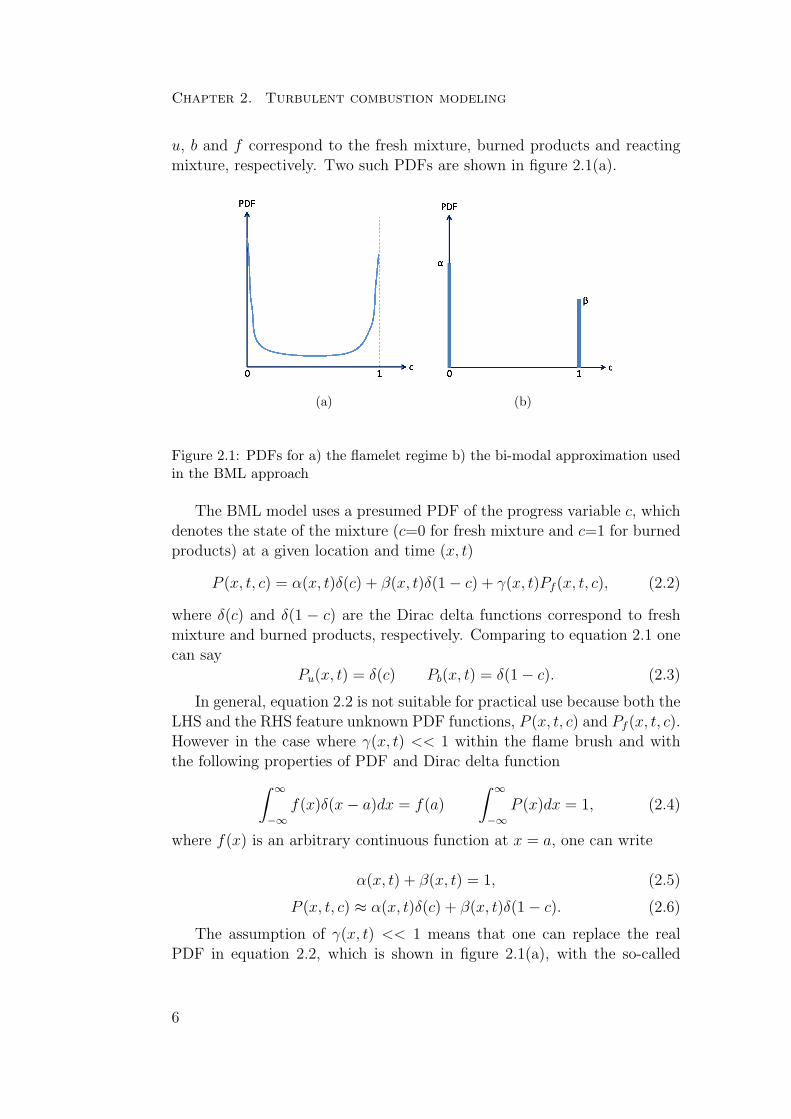
u, b and f correspond to the fresh mixture, burned products and reactingmixture, respectively. Two such PDFs are shown in figure 2.1(a).
(a) (b)
Figure 2.1: PDFs for a) the flamelet regime b) the bi-modal approximation usedin the BML approach
The BML model uses a presumed PDF of the progress variable c, whichdenotes the state of the mixture (c=0 for fresh mixture and c=1 for burnedproducts) at a given location and time (x, t)
P (x, t, c) = α(x, t)δ(c) + β(x, t)δ(1 − c) + γ(x, t)Pf (x, t, c), (2.2)
where δ(c) and δ(1 − c) are the Dirac delta functions correspond to freshmixture and burned products, respectively. Comparing to equation 2.1 onecan say
Pu(x, t) = δ(c) Pb(x, t) = δ(1 − c). (2.3)
In general, equation 2.2 is not suitable for practical use because both theLHS and the RHS feature unknown PDF functions, P (x, t, c) and Pf (x, t, c).However in the case where γ(x, t) << 1 within the flame brush and withthe following properties of PDF and Dirac delta function
∫ ∞
−∞
f(x)δ(x − a)dx = f(a)
∫ ∞
−∞
P (x)dx = 1, (2.4)
where f(x) is an arbitrary continuous function at x = a, one can write
α(x, t) + β(x, t) = 1, (2.5)
P (x, t, c) ≈ α(x, t)δ(c) + β(x, t)δ(1 − c). (2.6)
The assumption of γ(x, t) << 1 means that one can replace the realPDF in equation 2.2, which is shown in figure 2.1(a), with the so-called
6
2.2. Introduction to the BML approach
bi-modal PDF, equation 2.6. The bi-modal PDF consists of two Dirac deltafunctions at c=0 and c=1 and is shown in figure 2.1(b). α(x, t) and β(x, t)in equation 2.6 are unknown, and so the objective becomes to determinethe values of these parameters.
For any arbitrary function f(c)
f(c) =
∫ ∞
−∞
f(c)P (x, t, c)dc, (2.7)
One can therefore derive the following based on the properties of thePDF and the Dirac functions used in equation 2.4
c(x, t) =
∫ ∞
−∞
c(x, t)P (x, t, c)dc
=
∫1
0
c(x, t)[α(x, t)δ(c) + β(x, t)δ(1 − c)]dc
= α(x, t)c(x, t)c=0 + β(x, t)c(x, t)c=1
= β(x, t),
(2.8)
This shows that c is equal to the probability of finding burned products,and therefore
α = 1 − c(x, t). (2.9)
For the sake of simplicity, c(x, t), P (x, t, c), α(x, t) and β(x, t) are re-placed by c, P (c), α and β in the following discussion.
In general, for an arbitrary quantity, X, one can write
X = αXu + βXb = (1 − c)Xu + cXb, (2.10)
ρc = ρc =
∫1
0
ρcP (c)dc = α.(ρc)c=0 + β.(ρc)c=1 = ρbβ, (2.11)
and
ρ =
∫1
0
ρP (c)dc = α.(ρ)c=0 + β.(ρc)c=1
= αρu + βρb
= (1 − c)ρu + cρb.
(2.12)
where the overbar and overtilde represent the Reynolds and Favre averages,respectively. The relevance of these quantities is discussed in the followingsection.
7
Chapter 2. Turbulent combustion modeling
2.3 Reynolds and Favre averaging
This section introduces Reynolds and Favre averaging, and explains Favreaveraging is preferred to the more common Reynolds average in combustionsimulations. Reynolds averaging is widely used to analyze non-reactingflows, where there are no fluctuations in flow density. Based on the definitionof the Reynolds average, an arbitrary quantity such as X can be split intoa mean value X and a deviation from the mean, X ′
X = X + X ′, X ′ = 0 (2.13)
and for a statistically stationary process, X is defined as
X =1
∆t
∫∆t
0
Xdt, (2.14)
where ∆t is a time interval. This type of averaging can be applied tothe instantaneous balance equations, giving the Reynolds Averaged Naiver-Stokes(RANS) equations.
However in reacting flows, heat release causes fluctuations in density andtherefore Reynolds averaging produces an extra un-closed term. Indeed
∂ρ
∂t+
∂ρuj
∂xj
= 0 ⇒∂ρ
∂t+
∂(ρ + ρ′)(uj + u′j)
∂xj
= 0 ⇒
∂ρ
∂t+
∂ρuj + ρ′u′j
∂xj
= 0,
(2.15)
where the overlines denote the Reynolds averages and ρ′u′j is an unknown
term that can only be closed by modeling. These unclosed terms can beavoided by using Favre averaging instead
X =ρX
ρ, (2.16)
where ρ is the Reynolds average density and the tilde denotes Favre aver-aging. From the above, it follows that
X = X + X′′
, X ′′ = 0, X ′′ 6= 0. (2.17)
No extra unknown terms are created when the instantaneous mass con-servation equation is subjected to Favre averaging. Indeed
∂ρ
∂t+
∂ρuj
∂xj
= 0 ⇒∂ρ
∂t+
∂ρuj
∂xj
= 0. (2.18)
8
2.4. The governing equation
Therefore, for all transport equations that are commonly used in com-bustion simulations, Favre averaging is used in preference to Reynolds av-eraging. The next section presents some of the Favre-averaged balanceequations used in this work.
By applying the definition of the Favre average and combining equations2.8, 2.9, 2.11 and 2.12, one obtains the following
ρ =ρu
1 + (σ − 1)c, (2.19)
where σ = ρu/ρb is the density ratio
c =σc
1 + (σ − 1)c. (2.20)
Equation 2.20 is used to convert Favre-averaged progress values intotheir Reynolds-averaged equivalents.
2.4 The governing equation
As discussed in the previous section, Favre averaging is generally used incombustion simulations where the density of the reacting flow fluctuatessignificantly. This section presents the Favre-averaged balance equationsfor mass, momentum, and the progress variable.
• Mass:
∂ρ
∂t+
∂ρuj
∂xj
= 0, (2.21)
• Momentum:
∂ρui
∂t+
∂ρujui
∂xj
= −∂p
∂xi
+ µ∂2uj
∂xj∂xj
−∂τij
∂xj
, (2.22)
where τij = ρu′′j u
′′i is the Reynolds stresses tensor.
• Progress variable:
∂ρc
∂t+
∂(ρuj c)
∂xj
= −∂
∂xj
(ρu′′j c
′′) + ρW . (2.23)
In these equations, t is time while xj and uj are the coordinate and veloc-ity components, respectively. ρ is the mean density; in the BML framework,this is computed using equation 2.19. p and µ are the pressure and dynamicviscosity, respectively, and c is the progress variable (where a value of c=0
9
Chapter 2. Turbulent combustion modeling
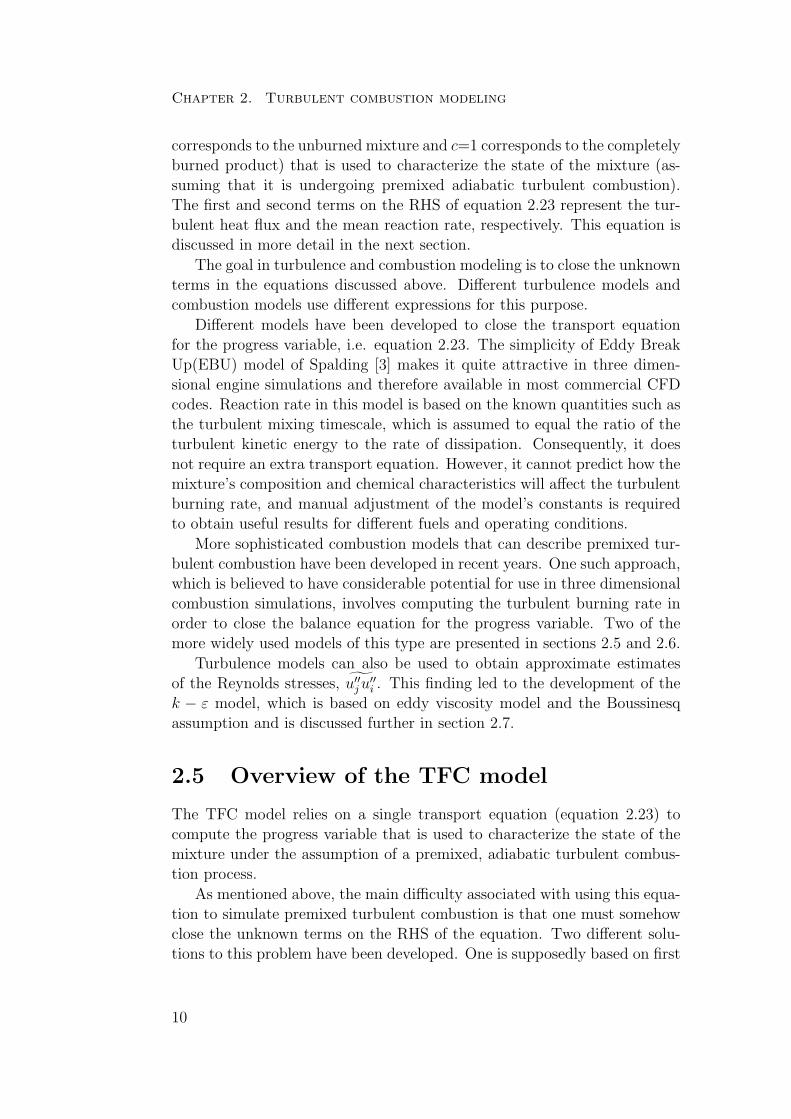
corresponds to the unburned mixture and c=1 corresponds to the completelyburned product) that is used to characterize the state of the mixture (as-suming that it is undergoing premixed adiabatic turbulent combustion).The first and second terms on the RHS of equation 2.23 represent the tur-bulent heat flux and the mean reaction rate, respectively. This equation isdiscussed in more detail in the next section.
The goal in turbulence and combustion modeling is to close the unknownterms in the equations discussed above. Different turbulence models andcombustion models use different expressions for this purpose.
Different models have been developed to close the transport equationfor the progress variable, i.e. equation 2.23. The simplicity of Eddy BreakUp(EBU) model of Spalding [3] makes it quite attractive in three dimen-sional engine simulations and therefore available in most commercial CFDcodes. Reaction rate in this model is based on the known quantities such asthe turbulent mixing timescale, which is assumed to equal the ratio of theturbulent kinetic energy to the rate of dissipation. Consequently, it doesnot require an extra transport equation. However, it cannot predict how themixture’s composition and chemical characteristics will affect the turbulentburning rate, and manual adjustment of the model’s constants is requiredto obtain useful results for different fuels and operating conditions.
More sophisticated combustion models that can describe premixed tur-bulent combustion have been developed in recent years. One such approach,which is believed to have considerable potential for use in three dimensionalcombustion simulations, involves computing the turbulent burning rate inorder to close the balance equation for the progress variable. Two of themore widely used models of this type are presented in sections 2.5 and 2.6.
Turbulence models can also be used to obtain approximate estimatesof the Reynolds stresses, u′′
j u′′i . This finding led to the development of the
k − ε model, which is based on eddy viscosity model and the Boussinesqassumption and is discussed further in section 2.7.
2.5 Overview of the TFC model
The TFC model relies on a single transport equation (equation 2.23) tocompute the progress variable that is used to characterize the state of themixture under the assumption of a premixed, adiabatic turbulent combus-tion process.
As mentioned above, the main difficulty associated with using this equa-tion to simulate premixed turbulent combustion is that one must somehowclose the unknown terms on the RHS of the equation. Two different solu-tions to this problem have been developed. One is supposedly based on first
10
2.5. Overview of the TFC model
principles while the other is more phenomenological.
While the first approach appears to have a more fundamental basis,the resulting expressions typically contain many unknown terms that mustbe closed by modeling. In addition, this approach often necessitates theinclusion of some constant whose universality is questionable, meaning thatthere is considerable scope for tuning. This approach will therefore requirefurther development before it will be ready for practical use.
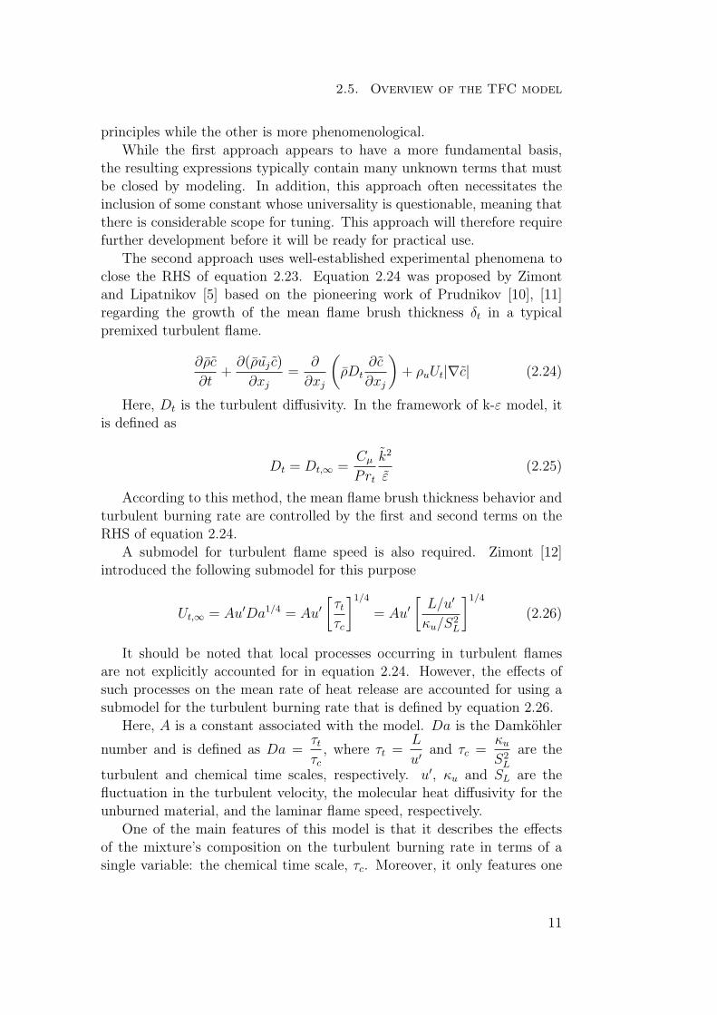
The second approach uses well-established experimental phenomena toclose the RHS of equation 2.23. Equation 2.24 was proposed by Zimontand Lipatnikov [5] based on the pioneering work of Prudnikov [10], [11]regarding the growth of the mean flame brush thickness δt in a typicalpremixed turbulent flame.
∂ρc
∂t+
∂(ρuj c)
∂xj
=∂
∂xj
(ρDt
∂c
∂xj
)+ ρuUt|∇c| (2.24)
Here, Dt is the turbulent diffusivity. In the framework of k-ε model, itis defined as
Dt = Dt,∞ =Cµ
Prt
k2
ε(2.25)
According to this method, the mean flame brush thickness behavior andturbulent burning rate are controlled by the first and second terms on theRHS of equation 2.24.
A submodel for turbulent flame speed is also required. Zimont [12]introduced the following submodel for this purpose
Ut,∞ = Au′Da1/4 = Au′
[τt
τc
]1/4
= Au′
[L/u′
κu/S2
L
]1/4
(2.26)
It should be noted that local processes occurring in turbulent flamesare not explicitly accounted for in equation 2.24. However, the effects ofsuch processes on the mean rate of heat release are accounted for using asubmodel for the turbulent burning rate that is defined by equation 2.26.
Here, A is a constant associated with the model. Da is the Damkohler
number and is defined as Da =τt
τc
, where τt =L
u′and τc =
κu
S2
L
are the
turbulent and chemical time scales, respectively. u′, κu and SL are thefluctuation in the turbulent velocity, the molecular heat diffusivity for theunburned material, and the laminar flame speed, respectively.
One of the main features of this model is that it describes the effectsof the mixture’s composition on the turbulent burning rate in terms of asingle variable: the chemical time scale, τc. Moreover, it only features one
11
Chapter 2. Turbulent combustion modeling
constant, making it a simple predictive tool that is quite straightforward touse in three dimensional simulations of premixed combustion processes.
An additional major strength of this approach is that a number of empir-ical trends derived from measurements of turbulent flame speed and burningvelocity, such as the tendency for Ut and the laminar flame speed to increaseduring turbulent velocity fluctuations, are accurately reproduced in simula-tions conducted using equation 2.26.
Equations 2.24 and 2.26 together comprise the Turbulent Flame Closure(TFC) model, which was derived by considering the intermediate transientregime that is characterized by a gradual increase in flame brush thicknesswith a constant turbulent burning velocity.
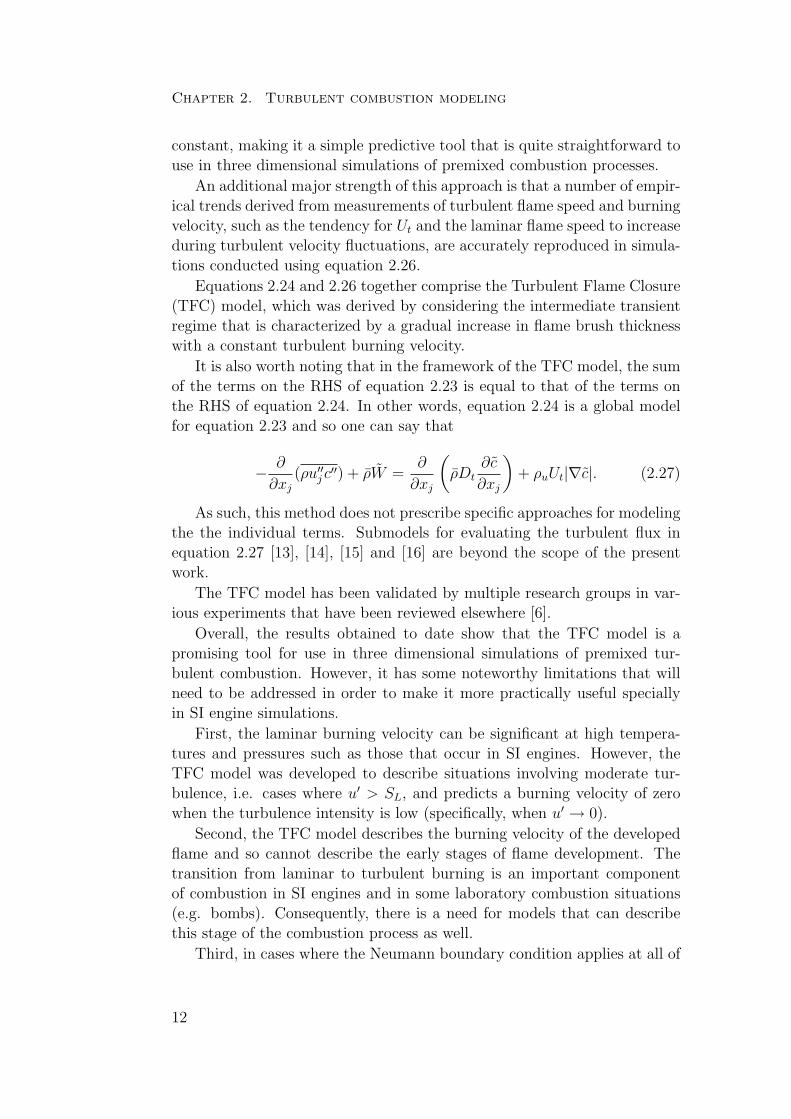
It is also worth noting that in the framework of the TFC model, the sumof the terms on the RHS of equation 2.23 is equal to that of the terms onthe RHS of equation 2.24. In other words, equation 2.24 is a global modelfor equation 2.23 and so one can say that
−∂
∂xj
(ρu′′j c
′′) + ρW =∂
∂xj
(ρDt
∂c
∂xj
)+ ρuUt|∇c|. (2.27)
As such, this method does not prescribe specific approaches for modelingthe the individual terms. Submodels for evaluating the turbulent flux inequation 2.27 [13], [14], [15] and [16] are beyond the scope of the presentwork.
The TFC model has been validated by multiple research groups in var-ious experiments that have been reviewed elsewhere [6].
Overall, the results obtained to date show that the TFC model is apromising tool for use in three dimensional simulations of premixed tur-bulent combustion. However, it has some noteworthy limitations that willneed to be addressed in order to make it more practically useful speciallyin SI engine simulations.
First, the laminar burning velocity can be significant at high tempera-tures and pressures such as those that occur in SI engines. However, theTFC model was developed to describe situations involving moderate tur-bulence, i.e. cases where u′ > SL, and predicts a burning velocity of zerowhen the turbulence intensity is low (specifically, when u′ → 0).
Second, the TFC model describes the burning velocity of the developedflame and so cannot describe the early stages of flame development. Thetransition from laminar to turbulent burning is an important componentof combustion in SI engines and in some laboratory combustion situations(e.g. bombs). Consequently, there is a need for models that can describethis stage of the combustion process as well.
Third, in cases where the Neumann boundary condition applies at all of
12
2.6. Overview of the FSC model
the system’s boundaries, any c = const can be a solution of equation 2.24.These limitations are addressed in the FSC model, which is discussed in
2.6.
2.6 Overview of the FSC model
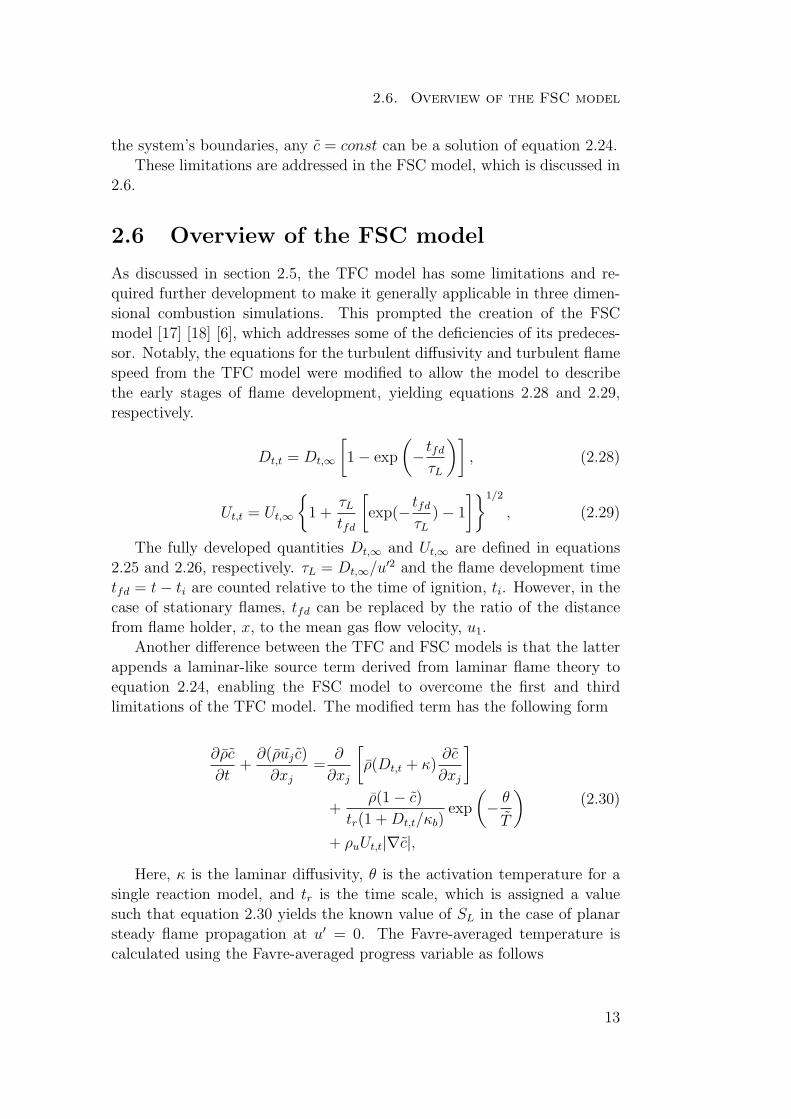
As discussed in section 2.5, the TFC model has some limitations and re-quired further development to make it generally applicable in three dimen-sional combustion simulations. This prompted the creation of the FSCmodel [17] [18] [6], which addresses some of the deficiencies of its predeces-sor. Notably, the equations for the turbulent diffusivity and turbulent flamespeed from the TFC model were modified to allow the model to describethe early stages of flame development, yielding equations 2.28 and 2.29,respectively.
Dt,t = Dt,∞
[1 − exp
(−
tfd
τL
)], (2.28)
Ut,t = Ut,∞
{1 +
τL
tfd
[exp(−
tfd
τL
) − 1
]}1/2
, (2.29)
The fully developed quantities Dt,∞ and Ut,∞ are defined in equations2.25 and 2.26, respectively. τL = Dt,∞/u′2 and the flame development timetfd = t − ti are counted relative to the time of ignition, ti. However, in thecase of stationary flames, tfd can be replaced by the ratio of the distancefrom flame holder, x, to the mean gas flow velocity, u1.
Another difference between the TFC and FSC models is that the latterappends a laminar-like source term derived from laminar flame theory toequation 2.24, enabling the FSC model to overcome the first and thirdlimitations of the TFC model. The modified term has the following form
∂ρc
∂t+
∂(ρuj c)
∂xj
=∂
∂xj
[ρ(Dt,t + κ)
∂c
∂xj
]
+ρ(1 − c)
tr(1 + Dt,t/κb)exp
(−
θ
T
)
+ ρuUt,t|∇c|,
(2.30)
Here, κ is the laminar diffusivity, θ is the activation temperature for asingle reaction model, and tr is the time scale, which is assigned a valuesuch that equation 2.30 yields the known value of SL in the case of planarsteady flame propagation at u′ = 0. The Favre-averaged temperature iscalculated using the Favre-averaged progress variable as follows
13
Chapter 2. Turbulent combustion modeling
T = Tu.(1 − c + σc), (2.31)
where σ = ρu/ρb is the density ratio. It is clear that equation 2.30 canpredict the laminar burning velocity in the limit case of u′ = Dt,t = Ut,t = 0because under such conditions it reduces to the balance equation of thelaminar flame theory [19].
The FSC model [17] [18] [6] consists of equations 2.30 (with and withoutthe exponential source term), 2.28 and 2.29. Notably, it overcomes thelimitations of the TFC model without introducing any new constants.
2.7 Turbulence model
The transport equation for the kinetic energy in the standard k-ε model isas follows,
∂ρk
∂t+ uj
∂ρk
∂xj
= ρPk − ρε + Dkt . (2.32)
The first and second terms on the LHS describe the variation of thekinetic energy over time and due to convection, respectively. Pk is theproduction term and must be computed by modeling due to the presence ofthe Reynolds stress tensor, which is unknown. In the linear eddy viscositymodel, Reynolds stresses are modeled using the Boussinesq assumption,yielding the following expression for Pk
Pk = −u′iu
′j
∂ui
∂xj
= νt
(∂ui
∂xj
+∂uj
∂xi
)∂ui
∂xj
= 2νtSijSij, (2.33)
where Sij is the symmetric part of the velocity gradient tensor and is definesas follows
Sij =1
2
(∂ui
∂xj
+∂uj
∂xi
). (2.34)
The second term on the RHS of the k equation is the dissipation term;its value is obtained from the dissipation term of the transport equation(i.e. equation 2.36).
Dkt in equation 2.32 is the turbulent diffusion term and must be modeled.
Based on the gradient hypothesis, this term can be modeled using equation2.35.
Dkt = −
∂
∂xj
(ρ
νt
σk
∂k
∂xj
). (2.35)
14
2.8. Dissipation and Prandtl number tuning
The modeled dissipation transport equation reads
∂ρε
∂t+ uj
∂ρε
∂xj
= ρε
k(cε1Pk − cε2ε) +
∂
∂xj
[ρ
νt
σε
∂ε
∂xj
]− cε3ρε
∂ui
∂xi
. (2.36)
The constants used in the k-ε model are as follows
σk = 1 σε = 1.3 cε1 = 1.44 cε2 = 1.92 cε3 = −0.33 (2.37)
In the standard k-ε model, cε3 = 0.The νt term in the k equation represents the turbulent viscosity and is
defined as
νt = cµk2
ε(2.38)
where the constant cµ is equal to 0.09.All of the transport equations used in this work have been presented and
discussed in this section and the two that preceded it. The following sectionprovides a brief overview of the algorithm used to solve these equations. Thebalance equations for velocity and pressure are solved using an iterativealgorithm of the type used in the incompressible case. However, becausethe density is not constant, it is calculated using equation 2.19 and thevalues of c are obtained by solving equation 2.24. The basic procedure is asfollows:
• Solving the velocity equation with an initial guess for pressure
• Solve for the progress variable by using the velocity field obtained fromprevious step and calculating the density of the reacting mixture
• Solve the Poisson equation for pressure using the velocity field ob-tained in the previous step
• Correct the velocity field with the new pressure field
• Repeat the steps above until the solution converges
2.8 Dissipation and Prandtl number tuning
As mentioned in the previous sections, there is in principle only one constant(A) to be tuned in both the TFC and FSC models. However, some addi-tional tuning may be required even if A is held constant. In order to evaluatethe predicted flow fields generated using combustion models, it is necessary
15
Chapter 2. Turbulent combustion modeling
to perform some modeling using turbulence models. This introduces twonotable sources of uncertainty when dealing with RANS simulations. Thefirst relates to the rate of dissipation at the boundary while the second isassociated with the turbulent Prandtl number, Prt. This section discussesthese uncertainties and describes methods for addressing them that havebeen proposed by different research groups.
To simulate a turbulent flow using the k-ε model, one must know thevalue of ε at the inlet boundary. However this value is not generally reportedin experimental papers; at best, a value for the length scale will be reportedbut not defined. If the value of the length scale is known, the dissipationrate can be calculated using equation 2.39, where L is the integral lengthscale.
ε =CDk3/2
L(2.39)
However, it is not clear what integral length scale should be substitutedin this equation, and different length scales yield substantially differentresults. For example, according to Shchetnikov [20], in a fully developedturbulent flow in a tube,
LL = 0.02d ; LE = 0.04d (2.40)
where LL and LE are the Lagrangian and Eulerian length scales, respec-tively, and d is the tube diameter. However it is not clear whether it is thelongitudinal, LE,‖, or transversal, LE,⊥, Eulerian length scale that is meanthere.
In homogeneous isotropic turbulence, LE,‖ = 2LE,⊥. Therefore, thelength scale in equation 2.39 cannot be greater than 0.08d if LE,⊥ = 2LL,i.e. LE,‖/LL < 8. However, Brodkey found that the inverse of this ratio canrange from 2 to 6.5. [21]
These uncertainties regarding the length scale introduce uncertainty intothe value of the constant used in equation 2.39. For example, Pope [22]suggested the following equation
ε = 0.43k3/2
LE,‖
≈ 0.77u′3
LE,‖
(2.41)
However, Dahms et al. [23] invoked ε = 0.37u′3
L.
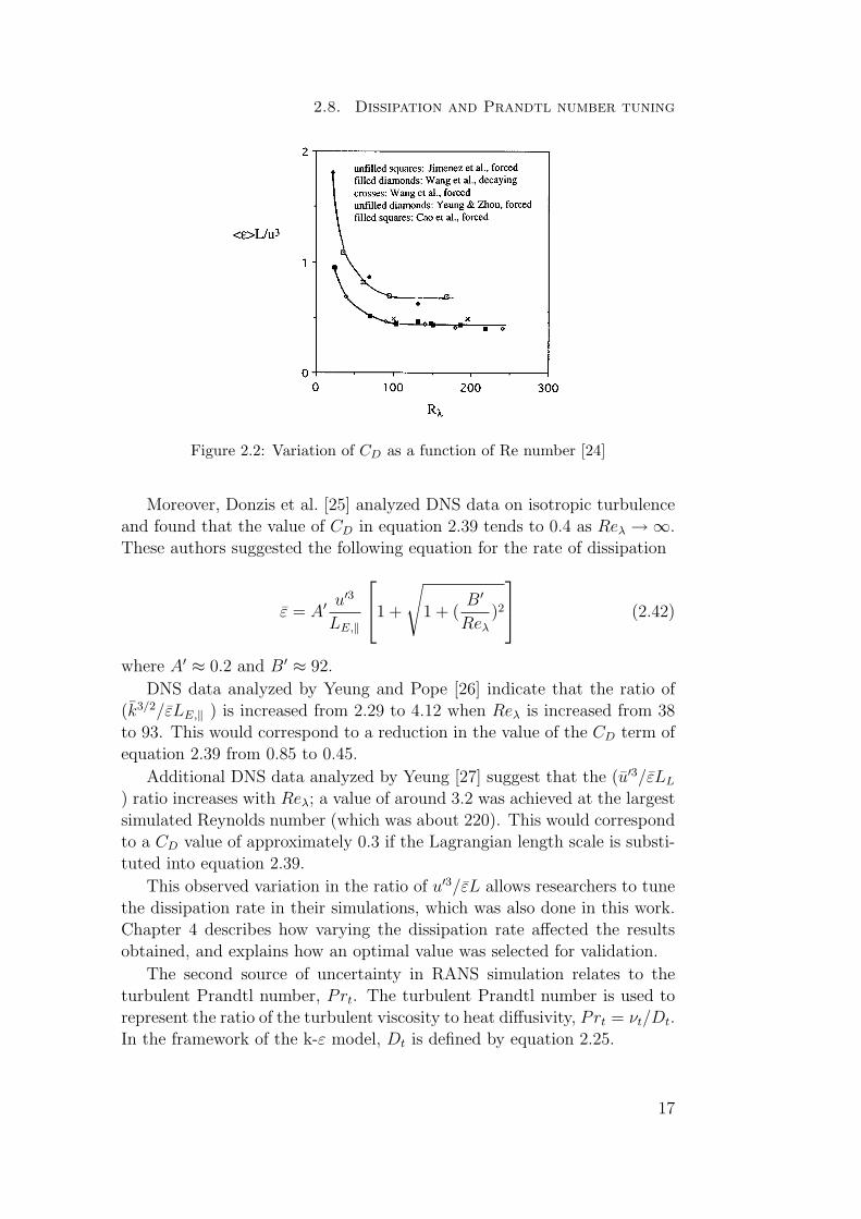
Moreover, DNS data analyzed by Sreenivasan [24] indicate that CD de-pends on the nature of the forcing applied at low wave numbers and on theRe number, as shown in figure 2.2. In this case, CD increases rapidly whenthe Taylor microscale Reynolds number, Reλ, is decreased.
16
2.8. Dissipation and Prandtl number tuning
Figure 2.2: Variation of CD as a function of Re number [24]
Moreover, Donzis et al. [25] analyzed DNS data on isotropic turbulenceand found that the value of CD in equation 2.39 tends to 0.4 as Reλ → ∞.These authors suggested the following equation for the rate of dissipation
ε = A′ u′3
LE,‖
1 +
√1 + (
B′
Reλ
)2
(2.42)
where A′ ≈ 0.2 and B′ ≈ 92.
DNS data analyzed by Yeung and Pope [26] indicate that the ratio of(k3/2/εLE,‖ ) is increased from 2.29 to 4.12 when Reλ is increased from 38to 93. This would correspond to a reduction in the value of the CD term ofequation 2.39 from 0.85 to 0.45.
Additional DNS data analyzed by Yeung [27] suggest that the (u′3/εLL
) ratio increases with Reλ; a value of around 3.2 was achieved at the largestsimulated Reynolds number (which was about 220). This would correspondto a CD value of approximately 0.3 if the Lagrangian length scale is substi-tuted into equation 2.39.
This observed variation in the ratio of u′3/εL allows researchers to tunethe dissipation rate in their simulations, which was also done in this work.Chapter 4 describes how varying the dissipation rate affected the resultsobtained, and explains how an optimal value was selected for validation.
The second source of uncertainty in RANS simulation relates to theturbulent Prandtl number, Prt. The turbulent Prandtl number is used torepresent the ratio of the turbulent viscosity to heat diffusivity, Prt = νt/Dt.In the framework of the k-ε model, Dt is defined by equation 2.25.
17
Chapter 2. Turbulent combustion modeling
The available data on the Prt number are controversial; typical valuesused in commercial CFD packages are 0.7 and 0.9, based on the work doneby Spalding [28] and Launder [29], respectively.
However these values are not universally accepted. For example, Reynolds[30] argued that the Prt number depends on the ratio of the eddy and kine-matic viscosities and the normal distance to the wall. Moreover, Koeltzsch[31] conducted wind tunnel experiments to examine a turbulent boundarylayer above a flat plate and found out that the Sct number (i.e. the ratioof the turbulent viscosity to the mass diffusivity) ranged from 0.3 to 1.
Similarly, Flesch [32] reported that the mean value of the Sct numberwas 0.6 but that its standard deviation was 52%. In other words, theirdata indicated that the Sct number varies from 0.18 to 1.34. The authorssuggested that some of this variation could be due to measurement uncer-tainty. However, they also argued that at least some of it was due to genuinevariation in the Sct number.
Bilger et al. [33] obtained a value of Pr = 0.35 based on an exper-imental study of a reaction in a scalar mixing layer that was subject togrid-generated turbulence. Moreover, Yeung [27] has proposed equation2.43
C0 =4
3
kε
τL
=8
9
Prt
Cµ
, (2.43)
C0 tends to take a value of 6.4 at large Reynolds numbers but is ap-proximately halved at low Re numbers, which are common in laboratoryexperiments involving premixed turbulent flames. This would yield a rela-tively low value for the Prt number according to equation 2.43. For example,while Prt = 0.65 if C0 = 6.4, its value can be as low as 0.3 in non-reactingflows. It should be noted that the typical values for the Prt number, 0.7and 0.9, were obtained by considering situations involving fully developedturbulent diffusivity that can be described by equation 2.25 under the as-sumption that t >> τL. However, since t/τL = O(1) for typical turbulentpremixed flames, a lower Prt number should be used in the FSC model (inwhich the turbulent diffusivity is calculated according to equation 2.28) inorder to achieve a diffusivity value equal to that predicted using equation2.25 and a Prt value of 0.7.
Due to these uncertainties in the value of the Prt number, it is easy tojustify tuning its value. Results obtained by such tuning are presented inchapter 4.
18
Chapter 3
Implementation of the models
3.1 Modification of the density calculation
procedure in OpenFOAM
As discussed previously, within the framework of the BML approach, thedensity is calculated using equation 2.19. The turbulent premixed solverused in OpenFOAM is based on the combustion regress variable, b = 1 −c. One would therefore expect the density to be calculated according toequation
1
ρ=
1
ρu
b +1
ρb
(1 − b) (3.1)
and the Favre-averaged temperature to be calculated as
T = Tub + Tb(1 − b) (3.2)
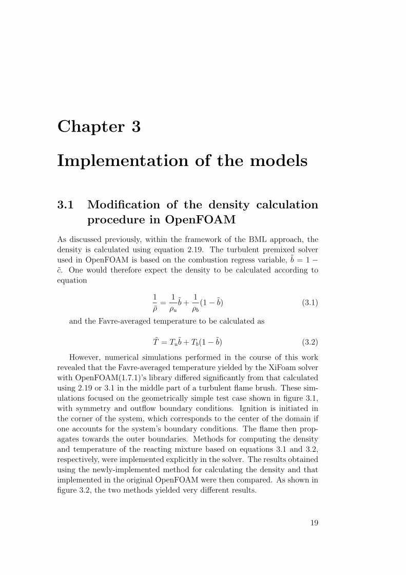
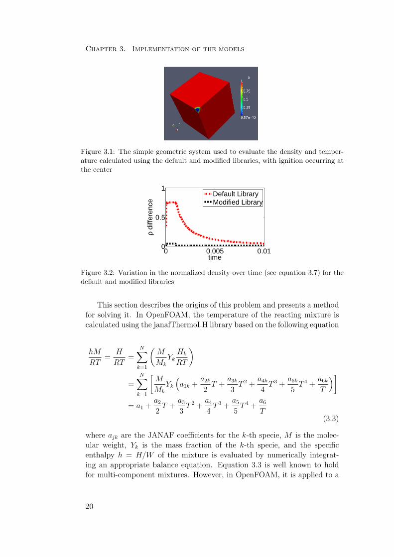
However, numerical simulations performed in the course of this workrevealed that the Favre-averaged temperature yielded by the XiFoam solverwith OpenFOAM(1.7.1)’s library differed significantly from that calculatedusing 2.19 or 3.1 in the middle part of a turbulent flame brush. These sim-ulations focused on the geometrically simple test case shown in figure 3.1,with symmetry and outflow boundary conditions. Ignition is initiated inthe corner of the system, which corresponds to the center of the domain ifone accounts for the system’s boundary conditions. The flame then prop-agates towards the outer boundaries. Methods for computing the densityand temperature of the reacting mixture based on equations 3.1 and 3.2,respectively, were implemented explicitly in the solver. The results obtainedusing the newly-implemented method for calculating the density and thatimplemented in the original OpenFOAM were then compared. As shown infigure 3.2, the two methods yielded very different results.
19
Chapter 3. Implementation of the models
Figure 3.1: The simple geometric system used to evaluate the density and temper-ature calculated using the default and modified libraries, with ignition occurring atthe center
0 0.005 0.010
0.5
1
time
ρ di
ffere
nce
Default LibraryModified Library
Figure 3.2: Variation in the normalized density over time (see equation 3.7) for thedefault and modified libraries
This section describes the origins of this problem and presents a methodfor solving it. In OpenFOAM, the temperature of the reacting mixture iscalculated using the janafThermoI.H library based on the following equation
hM
RT=
H
RT=
N∑
k=1
(M
Mk
YkHk
RT
)
=N∑
k=1
[M
Mk
Yk
(a1k +
a2k
2T +
a3k
3T 2 +
a4k
4T 3 +
a5k
5T 4 +
a6k
T
)]
= a1 +a2
2T +
a3
3T 2 +
a4
4T 3 +
a5
5T 4 +
a6
T(3.3)
where ajk are the JANAF coefficients for the k-th specie, M is the molec-ular weight, Yk is the mass fraction of the k-th specie, and the specificenthalpy h = H/W of the mixture is evaluated by numerically integrat-ing an appropriate balance equation. Equation 3.3 is well known to holdfor multi-component mixtures. However, in OpenFOAM, it is applied to a
20
3.1. Modification of the density calculation procedure in OpenFOAM
fundamentally different situation in which the burned and unburned mix-ture are both present within the turbulent flame brush but are separatedby a thin flamelet. More specifically, the mean state of the mixture withinthe flame brush is considered to be a “super-mixture ”of the reactants andproducts. The mass fractions, Y1 and Y2, respectively, of the reactants andproducts within this mixture are assumed to be b and, 1 − b respectively.Accordingly, the molecular weight Mm and JANAF coefficients ajm for thesuper-mixture are initially determined as follows (see libraries homogeneous-Mixture.C, janafThermoI.H, specieI.H)
1
Mm
=1
Mr
b +1
Mp
(1 − b)ajm
Mm
=ajr
Mr
b +ajp
Mp
(1 − b) (3.4)
The Favre-averaged temperature is then evaluated using the followingequation (see libraries janafThermoI.H, specieThermoI.H)
hMm
RT= a1m +
a2m
2T +
a3m
3T 2 +
a4m
4T 3 +
a5m
5T 4 +
a6m
T(3.5)
Table 3.1 compares the multi-component approach and the OpenFOAMapproach. As was mentioned earlier, in the OpenFOAM approach, themass fractions Y1 and Y2 for the reactants and products are replaced bythe quantities b and 1 − b, which originate from the description of multi-component mixtures.
Multi-component approach OpenFOAM approach
am,k
Mm
=∑N
l=1al,k
Yl
Ml
am,k
Mm
=au,k
Mu
b +ab,k
Mb
(1 − b)
1
Mm
=∑N
l=1
Yl
Ml
1
Mm
=1
Mu
b +1
Mb
(1 − b)
h =R
Mm
(∑5
k=1
am,k
kT k + am,6
)h =
R
Mm
(∑5
k=1
am,k
kT k + am,6
)
Table 3.1: Comparison of the multi-component and OpenFOAM approaches tocalculating the temperature of the mixture
However, this approach has at least two important problems. First,multi-component gas mixtures are completely different to situations involv-ing reactant-product intermittency within turbulent flame brushes, and
21
Chapter 3. Implementation of the models
there is no justification for applying equation 3.3 in modeling the latterphenomenon. For example, all species within a multi-component gas havethe same temperature, whereas Tp 6= Tr in situations involving reactant-product intermittency is concerned. Moreover, the mean density of a multi-component mixture is calculated by
ρ =N∑
k=1
ρk = ρu + ρb (3.6)
However, as mentioned previously, in the BLM framework, the densityof the mixture is calculated using equation 2.19; in the case where Tp = Tr,this method would predict a mean density of ρ = ρu = ρb.
Second, the non-linear equation 3.3 does not commute with the processof taking a mean, i.e. the substitution of ρT n/ρ with T n in the averagedequation 3.3 results in substantial errors.
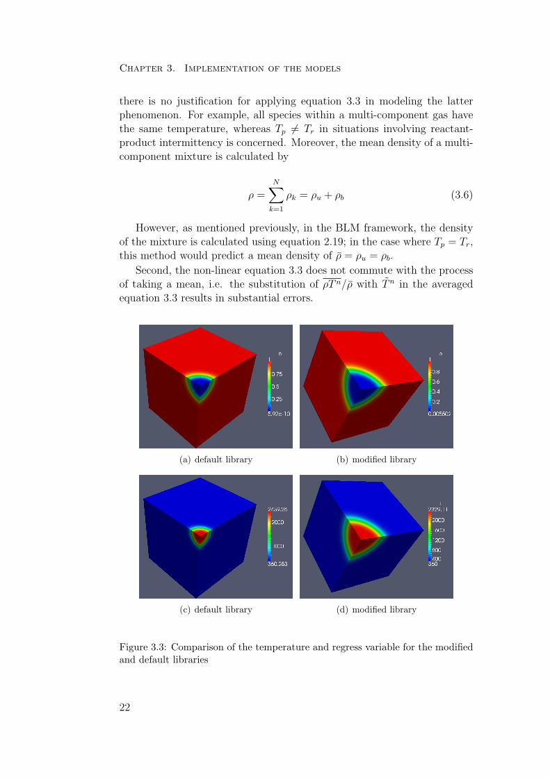
(a) default library (b) modified library
(c) default library (d) modified library
Figure 3.3: Comparison of the temperature and regress variable for the modifiedand default libraries
22
3.2. The implementation of the TFC and FSC models
To resolve this problem, the following method for evaluating T wasimplemented into the library hhuMixtureThermo.C of OpenFOAM. First,based on the local value of h obtained by numerically integrating an ap-propriate balance equation, the local values of Tu and Tb are determinedby applying equation 3.3 to the pure reactants and pure products, respec-tively. That is to say, Tu(Tb) is calculated using the reactant’s (or prod-uct’s) JANAF coefficients (see hhuMixtureThermo.C). Second, the Favre-averaged temperature is computed using equation 3.2.
The original and modified methods of calculating the Favre-averagedtemperature and density, were compared by calculating the following rela-tive error:
δρ ≡ max |ρOF (x, t) − ρ(x, t)
ρ(x, t)| (3.7)
Here, ρOF is the mean density obtained using the original OpenFOAMmethod; ρ is evaluated using equation 3.2, and the maximum is found inspace at each time step. Typical results obtained in this way are shown infigure 3.2. It is readily apparent that the modified approach yields a muchlower error than the original method, indicating that it is significantly moreaccurate.
Figure 3.3 shows the value of the temperature and the regress variable forboth the default and the modified libraries. When using the default library,the position of the flame front identified by analyzing the distribution oftemperatures is not the same as that determined by analysis of the regressvariable. Conversely, the two flame fronts are identical when using themodified library.
The next chapter describes two sets of simulations that were performedassuming adiabatic conditions. Therefore, a simpler version of the code wasimplemented in which the enthalpy equation is not solved and the densityis calculated directly according to equation 2.19, using ρu and ρb as inputvariables.
3.2 The implementation of the TFC and FSC
models
The XiFoam solver in OpenFOAM(1.7.1) is based on the transport equa-tion for the regress variable and solves enthalpy equations to calculate theunburned and burned temperatures. However, as mentioned in the previoussection, the simulated test cases were based on the assumption of adiabaticconditions. Therefore, the unburned and burned temperature were treated
23
Chapter 3. Implementation of the models
as input variables and there was no need to solve for the enthalpy. Thedefault solver supplied with OpenFOAM was therefore modified in order tobetter describe adiabatic situations.
In addition, the TFC model (including equations 2.24 and 2.26) wasimplemented in OpenFOAM.
fvScalarMatrix bEqn
(
fvm::ddt(rho, b)
+ mvConvection->fvmDiv(phi, b)
+ fvm::div(phiSt, b, "div(phiSt,b)")
- fvm::Sp(fvc::div(phiSt), b)
//------------modified---------------//
- fvm::laplacian(rho*Dt, b)
//---------------End-----------------//
);
where rho is the modified density as discussed in the previous section, b
is the regress variable, and phi is the velocity flux. rho∗Dt is the turbulentdiffusivity, which is calculated using equation 2.25 in the framework of thek-ε model, and phiSt is the turbulent flame speed flux; the turbulent flamespeed is calculated using equation 2.29
Ut = A*up*pow(Da,0.25); //[m/s]
here, A is the model constant, up is the fluctuation in the velocity, andDa is the Damkoler number.
In addition, the FSC model including equations 2.30, 2.29 and 2.28 wasimplemented in OpenFOAM as follows
fvScalarMatrix bEqn
(
fvm::ddt(rho, b)
+ mvConvection->fvmDiv(phi, b)
+ fvm::div(phiSt, b, "div(phiSt,b)")
- fvm::Sp(fvc::div(phiSt), b)
//------------modified---------------//
- fvm::laplacian( rho*Dtt, b) XX: laminar term
+ fvm::Sp(rho*Foam::exp(-activT/T_Tild)/(tr*(1+Dtt/alphab)), b)
//---------------End-----------------//
);
tr is the reaction time scale and phiSt is the turbulent flame speed flux.The turbulent flame speed and turbulent diffusivity are calculated usingequations 2.29 and 2.28, respectively.
24
Chapter 4
Model validation
4.1 Introduction
Simulations of Spark Ignition(SI) engines are complicated since they useseveral complex physical models (such as turbulence and ignition models),and must deal with numerical problems such as those arising from the useof moving meshes and complicated geometries. This means that they al-low for extensive tuning but also introduces multiple potential sources oferror. Thus, while SI engine simulations are extremely useful for studyingcombustion processes, they are not by themselves sufficient for testing theperformance of combustion models.
In order to further test the performance of the TFC and FSC models,they were therefore used to simulate two sets of experiments with simplegeometry and wide range of fuel-air mixtures and substantially different op-erating conditions that have been reported in the literature. The simulatedresults were compared to those obtained in practice. The first set of experi-mental results was obtained during a study on oblique, confined, preheated(600 K) and highly turbulent CH4-air flames with various equivalence ratios(Φ=0.62-1.24) that was conducted by Moreau [1]. The second experimentaldata set was obtained from a series of measurements of open, weakly tur-bulent, lean (Φ=0.5, 0.58, or 0.7) CH4-air V-shaped flames formed underambient conditions, and were performed by Dinkelacker and Holzler [2].
25
Chapter 4. Model validation
4.2 Highly turbulent confined flames
4.2.1 Simulated test case
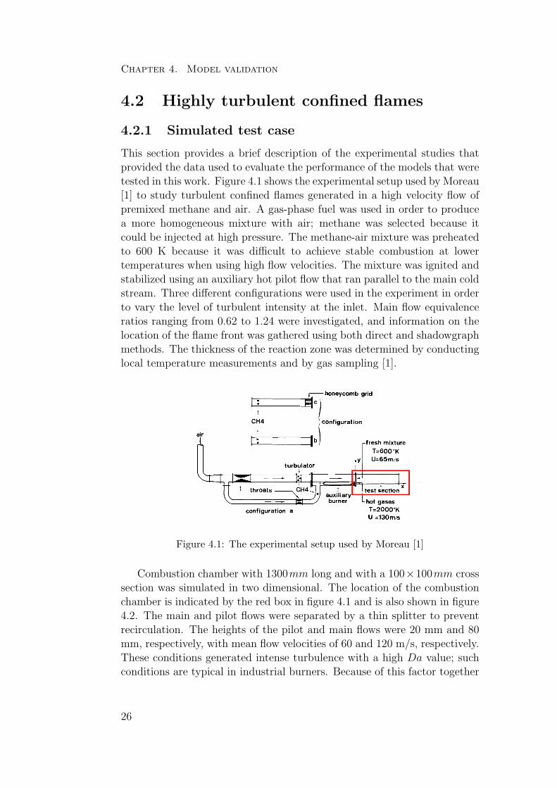
This section provides a brief description of the experimental studies thatprovided the data used to evaluate the performance of the models that weretested in this work. Figure 4.1 shows the experimental setup used by Moreau[1] to study turbulent confined flames generated in a high velocity flow ofpremixed methane and air. A gas-phase fuel was used in order to producea more homogeneous mixture with air; methane was selected because itcould be injected at high pressure. The methane-air mixture was preheatedto 600 K because it was difficult to achieve stable combustion at lowertemperatures when using high flow velocities. The mixture was ignited andstabilized using an auxiliary hot pilot flow that ran parallel to the main coldstream. Three different configurations were used in the experiment in orderto vary the level of turbulent intensity at the inlet. Main flow equivalenceratios ranging from 0.62 to 1.24 were investigated, and information on thelocation of the flame front was gathered using both direct and shadowgraphmethods. The thickness of the reaction zone was determined by conductinglocal temperature measurements and by gas sampling [1].
Figure 4.1: The experimental setup used by Moreau [1]
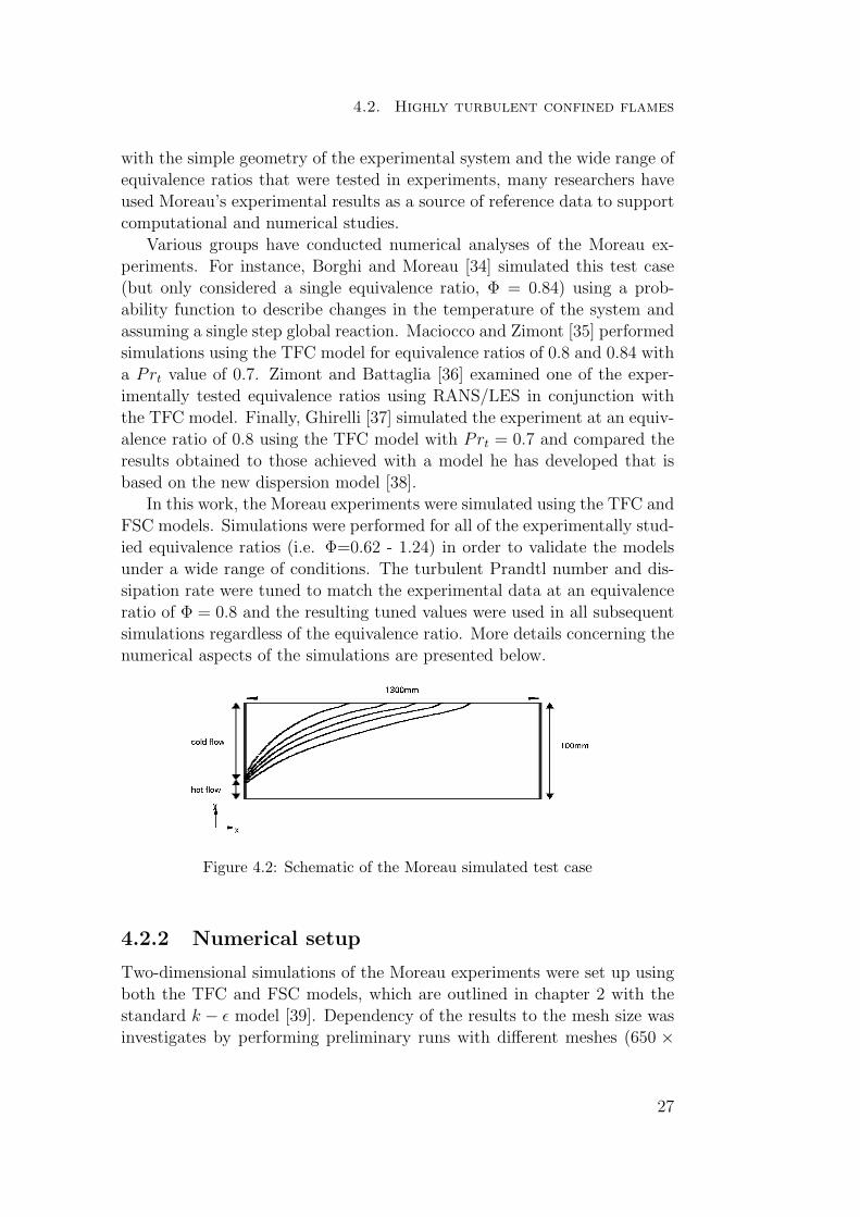
Combustion chamber with 1300mm long and with a 100×100mm crosssection was simulated in two dimensional. The location of the combustionchamber is indicated by the red box in figure 4.1 and is also shown in figure4.2. The main and pilot flows were separated by a thin splitter to preventrecirculation. The heights of the pilot and main flows were 20 mm and 80mm, respectively, with mean flow velocities of 60 and 120 m/s, respectively.These conditions generated intense turbulence with a high Da value; suchconditions are typical in industrial burners. Because of this factor together
26
4.2. Highly turbulent confined flames
with the simple geometry of the experimental system and the wide range ofequivalence ratios that were tested in experiments, many researchers haveused Moreau’s experimental results as a source of reference data to supportcomputational and numerical studies.
Various groups have conducted numerical analyses of the Moreau ex-periments. For instance, Borghi and Moreau [34] simulated this test case(but only considered a single equivalence ratio, Φ = 0.84) using a prob-ability function to describe changes in the temperature of the system andassuming a single step global reaction. Maciocco and Zimont [35] performedsimulations using the TFC model for equivalence ratios of 0.8 and 0.84 witha Prt value of 0.7. Zimont and Battaglia [36] examined one of the exper-imentally tested equivalence ratios using RANS/LES in conjunction withthe TFC model. Finally, Ghirelli [37] simulated the experiment at an equiv-alence ratio of 0.8 using the TFC model with Prt = 0.7 and compared theresults obtained to those achieved with a model he has developed that isbased on the new dispersion model [38].
In this work, the Moreau experiments were simulated using the TFC andFSC models. Simulations were performed for all of the experimentally stud-ied equivalence ratios (i.e. Φ=0.62 - 1.24) in order to validate the modelsunder a wide range of conditions. The turbulent Prandtl number and dis-sipation rate were tuned to match the experimental data at an equivalenceratio of Φ = 0.8 and the resulting tuned values were used in all subsequentsimulations regardless of the equivalence ratio. More details concerning thenumerical aspects of the simulations are presented below.
Figure 4.2: Schematic of the Moreau simulated test case
4.2.2 Numerical setup
Two-dimensional simulations of the Moreau experiments were set up usingboth the TFC and FSC models, which are outlined in chapter 2 with thestandard k − ǫ model [39]. Dependency of the results to the mesh size wasinvestigates by performing preliminary runs with different meshes (650 ×
27
Chapter 4. Model validation
50, 1300 × 120); ultimately, a uniform 325× 25 grid was identified as beingoptimal and was used in all of the simulations discussed below.
A range of numerical discretization schemes for the divergence term wereinvestigated but it was found that the results obtained were independent ofthe scheme used, so the limited second order central difference method wasselected for the convection term discretization.
T (K) k(m2/s2) c U(m/s) ρ(kg/m3)
cold flow 600 100 0 60 0.5603
hot flow T (Φ) 793 1 120 ρ(Φ)
Table 4.1: Inflow boundary conditions
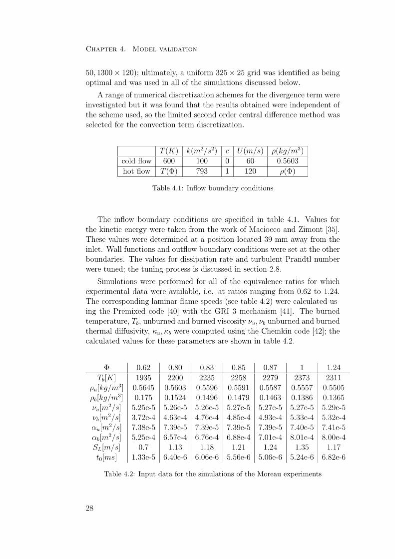
The inflow boundary conditions are specified in table 4.1. Values forthe kinetic energy were taken from the work of Maciocco and Zimont [35].These values were determined at a position located 39 mm away from theinlet. Wall functions and outflow boundary conditions were set at the otherboundaries. The values for dissipation rate and turbulent Prandtl numberwere tuned; the tuning process is discussed in section 2.8.
Simulations were performed for all of the equivalence ratios for whichexperimental data were available, i.e. at ratios ranging from 0.62 to 1.24.The corresponding laminar flame speeds (see table 4.2) were calculated us-ing the Premixed code [40] with the GRI 3 mechanism [41]. The burnedtemperature, Tb, unburned and burned viscosity νu, νb unburned and burnedthermal diffusivity, κu, κb were computed using the Chemkin code [42]; thecalculated values for these parameters are shown in table 4.2.
Φ 0.62 0.80 0.83 0.85 0.87 1 1.24
Tb[K] 1935 2200 2235 2258 2279 2373 2311ρu[kg/m3] 0.5645 0.5603 0.5596 0.5591 0.5587 0.5557 0.5505ρb[kg/m3] 0.175 0.1524 0.1496 0.1479 0.1463 0.1386 0.1365νu[m
2/s] 5.25e-5 5.26e-5 5.26e-5 5.27e-5 5.27e-5 5.27e-5 5.29e-5νb[m
2/s] 3.72e-4 4.63e-4 4.76e-4 4.85e-4 4.93e-4 5.33e-4 5.32e-4αu[m
2/s] 7.38e-5 7.39e-5 7.39e-5 7.39e-5 7.39e-5 7.40e-5 7.41e-5αb[m
2/s] 5.25e-4 6.57e-4 6.76e-4 6.88e-4 7.01e-4 8.01e-4 8.00e-4SL[m/s] 0.7 1.13 1.18 1.21 1.24 1.35 1.17t0[ms] 1.33e-5 6.40e-6 6.06e-6 5.56e-6 5.06e-6 5.24e-6 6.82e-6
Table 4.2: Input data for the simulations of the Moreau experiments
28
4.2. Highly turbulent confined flames
4.2.3 Results, validation, and discussion
The discussion of the results obtained in this work is subdivided into threemain sections, covering:
i) sensitivity analysis,ii) tuningiii) validation.
The first section describes investigations into the sensitivity of the resultsto three-dimensional effects, the identity of the turbulence model used, andthe velocity used to calculate the flame development time in the FSC model,t = x/u. As discussed extensively in section 2.8, it was necessary to tunethe values of Prt and ε that were used in the simulations. The secondsection explains the procedure used to tune these parameters for the TFCand FSC models, which involved considering a single equivalence ratio andvarying their values to identify those that yielded the closest agreement withthe experimental data in each case. The final section describes the resultsobtained in the simulations conducted for other equivalence ratios using thetuned values for Prt and the dissipation rate. The specific topics discussedin each section are listed below:
• Sensitivity Analysis:
1. A comparison of 2D and 3D simulations using the TFC model
2. The effect of varying the turbulence model on TFC simulations
3. The effect of varying the velocity parameter used to computet = x/u in the FSC model
• Tuning:
4. Effect of varying the dissipation rate on TFC simulations
5. Effect of varying the dissipation rate on FSC simulations
6. Effect of varying the Prt number on TFC simulations
7. Effect of varying the Prt number on FSC simulations
• Validation:
8. Comparison of the simulated results obtained using the TFC andFSC models, and the FSC model with an exponential source term
29
Chapter 4. Model validation
• Sensitivity Analysis:
1. A comparison of 2D and 3D simulations using the TFC model
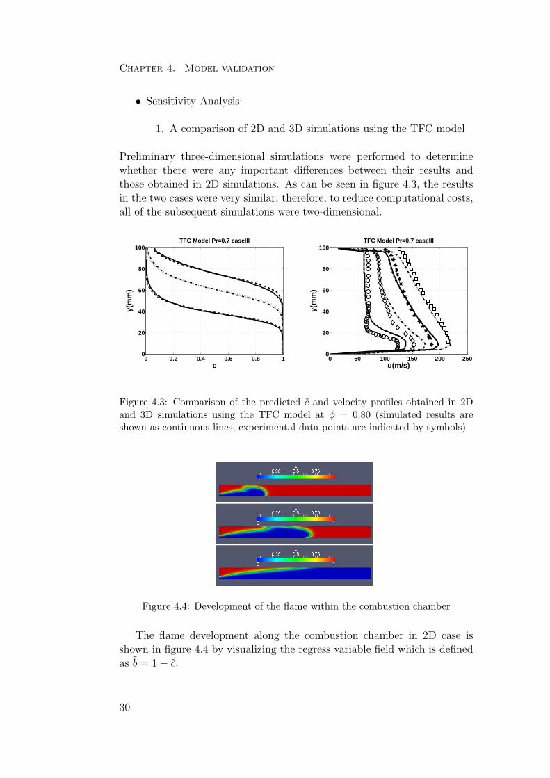
Preliminary three-dimensional simulations were performed to determinewhether there were any important differences between their results andthose obtained in 2D simulations. As can be seen in figure 4.3, the resultsin the two cases were very similar; therefore, to reduce computational costs,all of the subsequent simulations were two-dimensional.
0 0.2 0.4 0.6 0.8 10
20
40
60
80
100TFC Model Pr=0.7 caseIII
y(m
m)
c
0 50 100 150 200 2500
20
40
60
80
100
u(m/s)
y(m
m)
TFC Model Pr=0.7 caseIII
Figure 4.3: Comparison of the predicted c and velocity profiles obtained in 2Dand 3D simulations using the TFC model at φ = 0.80 (simulated results areshown as continuous lines, experimental data points are indicated by symbols)
Figure 4.4: Development of the flame within the combustion chamber
The flame development along the combustion chamber in 2D case isshown in figure 4.4 by visualizing the regress variable field which is definedas b = 1 − c.
30
4.2. Highly turbulent confined flames
• Sensitivity Analysis:
2. The effect of varying the turbulence model on TFC simulations
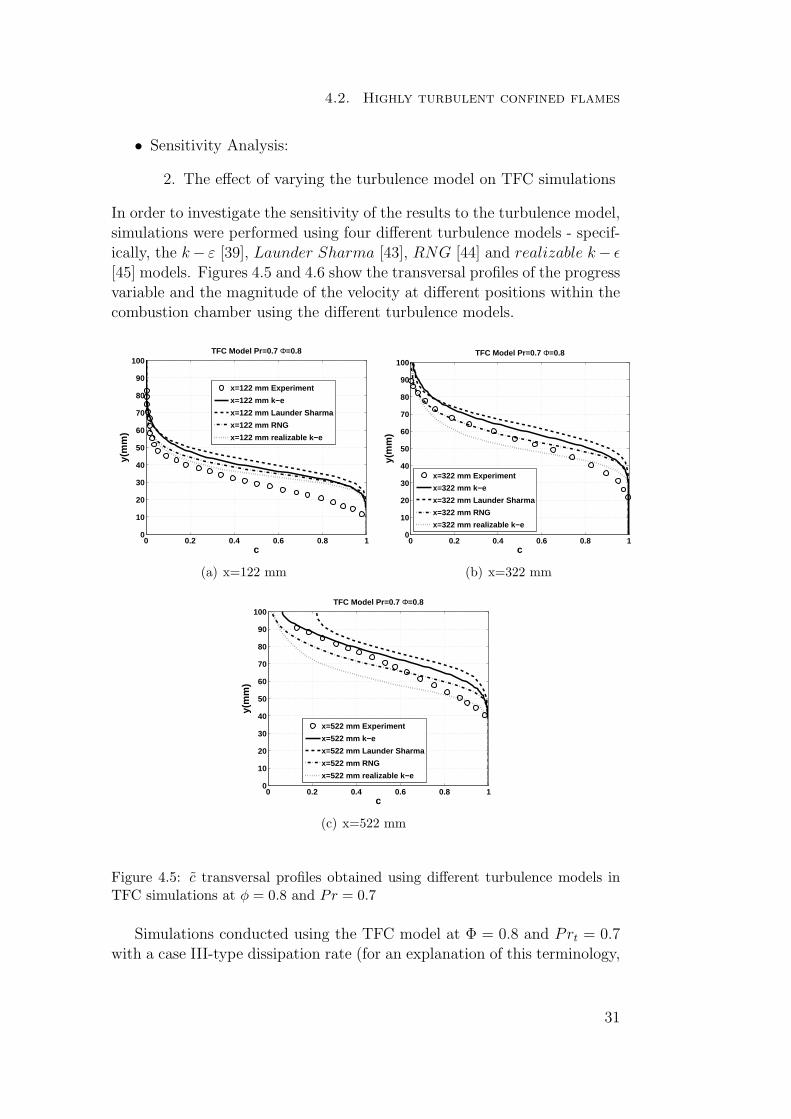
In order to investigate the sensitivity of the results to the turbulence model,simulations were performed using four different turbulence models - specif-ically, the k− ε [39], Launder Sharma [43], RNG [44] and realizable k− ǫ[45] models. Figures 4.5 and 4.6 show the transversal profiles of the progressvariable and the magnitude of the velocity at different positions within thecombustion chamber using the different turbulence models.
0 0.2 0.4 0.6 0.8 10
10
20
30
40
50
60
70
80
90
100
c
y(m
m)
TFC Model Pr=0.7 Φ=0.8
x=122 mm Experiment
x=122 mm k−e
x=122 mm Launder Sharma
x=122 mm RNG
x=122 mm realizable k−e
(a) x=122 mm
0 0.2 0.4 0.6 0.8 10
10
20
30
40
50
60
70
80
90
100
c
y(m
m)
TFC Model Pr=0.7 Φ=0.8
x=322 mm Experiment
x=322 mm k−e
x=322 mm Launder Sharma
x=322 mm RNG
x=322 mm realizable k−e
(b) x=322 mm
0 0.2 0.4 0.6 0.8 10
10
20
30
40
50
60
70
80
90
100
c
y(m
m)
TFC Model Pr=0.7 Φ=0.8
x=522 mm Experiment
x=522 mm k−e
x=522 mm Launder Sharma
x=522 mm RNG
x=522 mm realizable k−e
(c) x=522 mm
Figure 4.5: c transversal profiles obtained using different turbulence models inTFC simulations at φ = 0.8 and Pr = 0.7
Simulations conducted using the TFC model at Φ = 0.8 and Prt = 0.7with a case III-type dissipation rate (for an explanation of this terminology,
31
Chapter 4. Model validation
see table 4.3). The c profile clearly shows that the burning rate and flamebrush thickness are both sensitive to the turbulence model used.
Figure 4.5 shows that the Launder Sharma model consistently predictshigher burning rates than are obtained with the other turbulence models.Moreover, the predicted burning rates generated using this model tend tobe significantly greater than the experimental values. The realizable k − ǫmodel tends to predict relatively low burning rates, while the rates predictedby the k-ǫ and RNG models are intermediate between these two extremes.It is also apparent that the realizable k-ǫ model underpredicts the burningrate at the 322 mm and 522 mm positions. Overall, the results obtainedusing the RNG and k-ǫ models are closest to the experimental results.
0 50 100 1500
10
20
30
40
50
60
70
80
90
100
u(m/s)
y(m
m)
TFC Model Pr=0.7 Φ=0.8
x=39 mm Experiment
x=39 mm k−e
x=39 mm Launder Sharma
x=39 mm RNG
x=39 mm realizable k−e
(a) x=39 mm
0 50 100 150 2000
10
20
30
40
50
60
70
80
90
100
u(m/s)
y(m
m)
TFC Model Pr=0.7 Φ=0.8
x=251 mm Experiment
x=251 mm k−e
x=251 mm Launder Sharma
x=251 mm RNG
x=251 mm realizable k−e
(b) x=251 mm
0 50 100 150 200 2500
10
20
30
40
50
60
70
80
90
100
u(m/s)
y(m
m)
TFC Model Pr=0.7 Φ=0.8
x=438 mm Experiment
x=438 mm k−e
x=438 mm Launder Sharma
x=438 mm RNG
x=438 mm realizable k−e
(c) x=438 mm
0 50 100 150 200 250 3000
10
20
30
40
50
60
70
80
90
100
u(m/s)
y(m
m)
TFC Model Pr=0.7 Φ=0.8
x=650 mm Experiment
x=650 mm k−e
x=650 mm Launder Sharma
x=650 mm RNG
x=650 mm realizable k−e
(d) x=650 mm
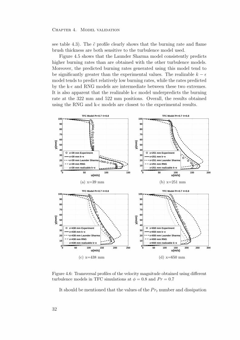
Figure 4.6: Transversal profiles of the velocity magnitude obtained using differentturbulence models in TFC simulations at φ = 0.8 and Pr = 0.7
It should be mentioned that the values of the Prt number and dissipation
32
4.2. Highly turbulent confined flames
rate had not been tuned at this point in the study, and it is possible thatthe use of tuned parameters might significantly affect the performance ofthe tested models.
The streamwise velocity profiles shown in figure 4.6 show that the Laun-der Sharma model overpredicts the magnitude of the flow velocity at the251 mm, 438 mm and 650 mm positions. Moreover, both the realizable k-ǫmodel and the RNG model underpredict the magnitude of the velocity atthe 438 mm and 650 mm positions. Overall, the results obtained with thek-ǫ model seem to have the best agreement with the experimental data.
The k-ǫ model performed better than the alternatives in terms of pre-dicting both the burning rate and the magnitude of the velocity and wastherefore used in all subsequent simulations.
• Sensitivity Analysis:
3. The effect of varying the velocity parameter used to computet = x/u in the FSC model
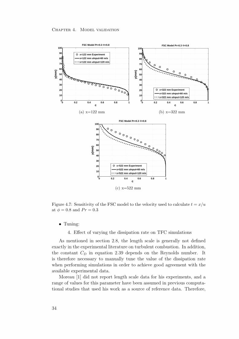
As discussed in chapter 2 and as shown by equations 2.29 and 2.28,the turbulent flame velocity and turbulent diffusivity are functions of timein the FSC model. However, the work presented herein focused on time-independent stationary cases. It was therefore necessary to redefine t in theFSC model. As was discussed in section 2.8, this was done by assumingthat t = x/u where x is the distance from the flame holder (or splitter inthis case) and u is the mean velocity.
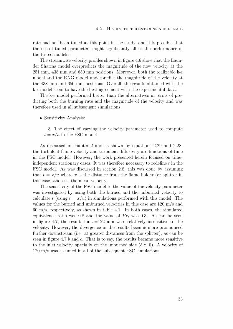
The sensitivity of the FSC model to the value of the velocity parameterwas investigated by using both the burned and the unburned velocity tocalculate t (using t = x/u) in simulations performed with this model. Thevalues for the burned and unburned velocities in this case are 120 m/s and60 m/s, respectively, as shown in table 4.1. In both cases, the simulatedequivalence ratio was 0.8 and the value of Prt was 0.3. As can be seenin figure 4.7, the results for x=122 mm were relatively insensitive to thevelocity. However, the divergence in the results became more pronouncedfurther downstream (i.e. at greater distances from the splitter), as can beseen in figure 4.7 b and c. That is to say, the results became more sensitiveto the inlet velocity, specially on the unburned side (c ≃ 0). A velocity of120 m/s was assumed in all of the subsequent FSC simulations.
33
Chapter 4. Model validation
0 0.2 0.4 0.6 0.8 10
10
20
30
40
50
60
70
80
90
100
c
y(m
m)
FSC Model Pr=0.3 Φ=0.8
x=122 mm Experiment
x=122 mm uInput=60 m/s
x=122 mm uInput=120 m/s
(a) x=122 mm
0 0.2 0.4 0.6 0.8 10
10
20
30
40
50
60
70
80
90
100
c
y(m
m)
FSC Model Pr=0.3 Φ=0.8
x=322 mm Experiment
x=322 mm uInput=60 m/s
x=322 mm uInput=120 m/s
(b) x=322 mm
0 0.2 0.4 0.6 0.8 10
10
20
30
40
50
60
70
80
90
100
c
y(m
m)
FSC Model Pr=0.3 Φ=0.8
x=522 mm Experiment
x=522 mm uInput=60 m/s
x=522 mm uInput=120 m/s
(c) x=522 mm
Figure 4.7: Sensitivity of the FSC model to the velocity used to calculate t = x/uat φ = 0.8 and Pr = 0.3
• Tuning:
4. Effect of varying the dissipation rate on TFC simulations
As mentioned in section 2.8, the length scale is generally not definedexactly in the experimental literature on turbulent combustion. In addition,the constant CD in equation 2.39 depends on the Reynolds number. Itis therefore necessary to manually tune the value of the dissipation ratewhen performing simulations in order to achieve good agreement with theavailable experimental data.
Moreau [1] did not report length scale data for his experiments, and arange of values for this parameter have been assumed in previous computa-tional studies that used his work as a source of reference data. Therefore,
34
4.2. Highly turbulent confined flames
simulations of the Moreau experiments at an equivalence ratio of 0.8 wereperformed using each of the four different length scales listed in table 4.3in order to identify an appropriate value for this parameter in subsequentTFC simulations. The four length scales are labeled cases I-IV to facilitatediscussion.
case I case II case III case IV
lu[mm] 24 8.21 5.4 2.7lb[mm] 6 1.83 1.6 0.8εum
2/s3 6.85e3 2e4 3.7e4 7.4e4εbm
2/s3 6.12e5 2e6 2.86e6 5.6e6
Table 4.3: The four different length scales considered and the associated inflowdissipation rates in (m2/s3)
The dissipation rates associated with each of the four tested length scalesshown in table 4.3 were calculated using equation 2.39. The length scaleused in case I is that reported by Zimont et.al [13]. Cases II and III assumelength scales based on the work of Ghirelli [37] and Maciocoo and Zimont[35], respectively. It should be noted here that Ghirielli considered non-isotropic turbulence in the study from which the case II length scale wastaken and therefore obtained a different value for the kinetic energy than wasfound in this work. The length scale used in case IV was chosen arbitrarilyand is twice that used in case III.
In order to investigate the effect of the dissipation rate on the TFCmodel, TFC simulations were conducted assuming Prt values of 0.3 and0.7 at an equivalence ratio of Φ = 0.80 using dissipation rates presentedin table 4.3. Figure 4.8 shows the results obtained at different positionswithin the combustion chamber (i.e. at different values of x) in each case.As the dissipation rate was increased on going from case I to case IV, thelevel of turbulent diffusion (which was calculated using equation 2.25) de-creased. This caused a decrease in the mean flame brush thickness, with acorresponding increase in the slopes of the curves shown in figure 4.8. Asdescribed by equation 2.39, increases in the the dissipation rate are associ-ated with decreases in the length scale of the system, which in turn reduce
the Da number(τt
τc
=L/u′
τc
). This reduces the burning rate, as described by
equation 2.26. Results consistent with these expectations were obtained atall positions within the combustion chamber, at both tested values of thePrandtl number. A summary of these trends is given by equations 4.1 and4.2.
ε ↑ =⇒ DT ↓ =⇒ Thickness ↓ (4.1)
35
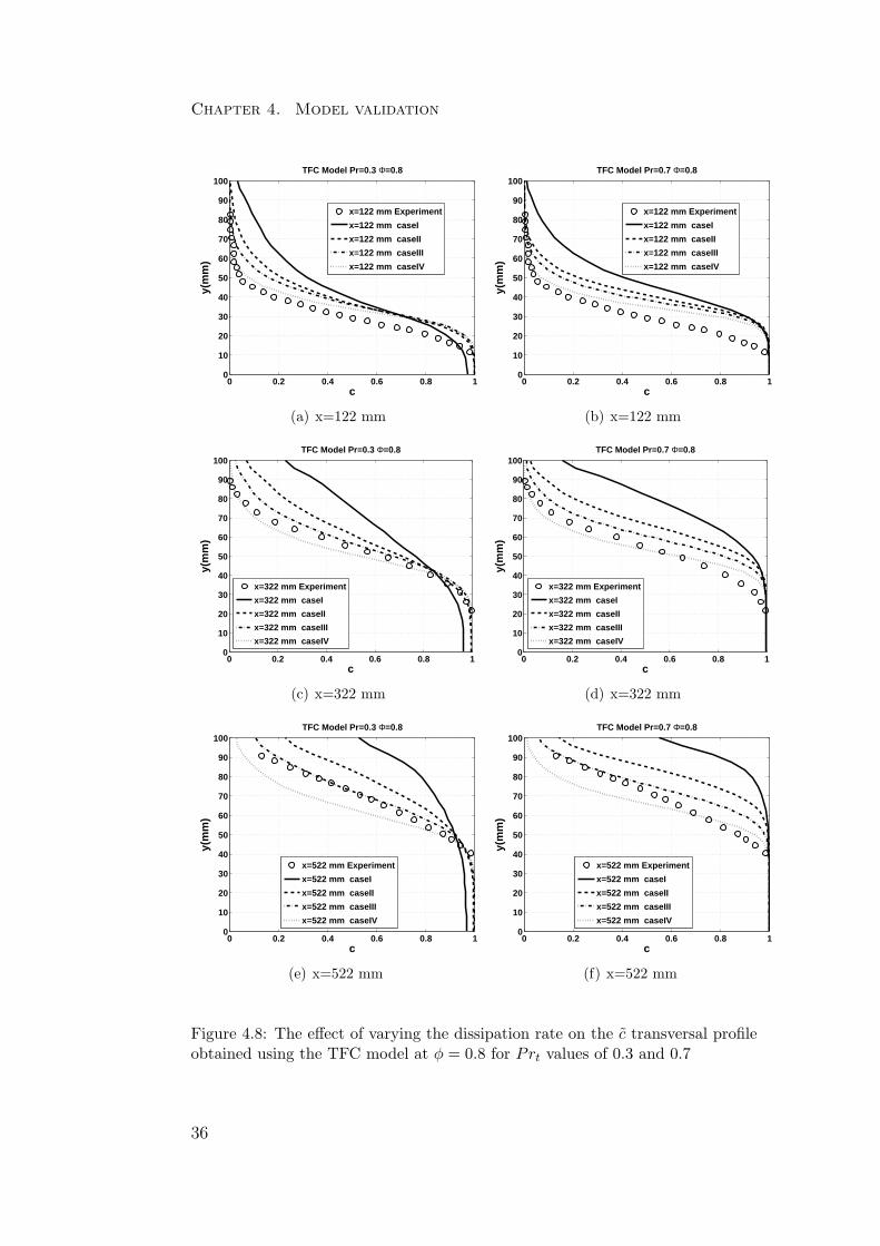
Chapter 4. Model validation
0 0.2 0.4 0.6 0.8 10
10
20
30
40
50
60
70
80
90
100
c
y(m
m)
TFC Model Pr=0.3 Φ=0.8
x=122 mm Experiment
x=122 mm caseI
x=122 mm caseII
x=122 mm caseIII
x=122 mm caseIV
(a) x=122 mm
0 0.2 0.4 0.6 0.8 10
10
20
30
40
50
60
70
80
90
100
c
y(m
m)
TFC Model Pr=0.7 Φ=0.8
x=122 mm Experiment
x=122 mm caseI
x=122 mm caseII
x=122 mm caseIII
x=122 mm caseIV
(b) x=122 mm
0 0.2 0.4 0.6 0.8 10
10
20
30
40
50
60
70
80
90
100
c
y(m
m)
TFC Model Pr=0.3 Φ=0.8
x=322 mm Experiment
x=322 mm caseI
x=322 mm caseII
x=322 mm caseIII
x=322 mm caseIV
(c) x=322 mm
0 0.2 0.4 0.6 0.8 10
10
20
30
40
50
60
70
80
90
100
c
y(m
m)
TFC Model Pr=0.7 Φ=0.8
x=322 mm Experiment
x=322 mm caseI
x=322 mm caseII
x=322 mm caseIII
x=322 mm caseIV
(d) x=322 mm
0 0.2 0.4 0.6 0.8 10
10
20
30
40
50
60
70
80
90
100
c
y(m
m)
TFC Model Pr=0.3 Φ=0.8
x=522 mm Experiment
x=522 mm caseI
x=522 mm caseII
x=522 mm caseIII
x=522 mm caseIV
(e) x=522 mm
0 0.2 0.4 0.6 0.8 10
10
20
30
40
50
60
70
80
90
100
c
y(m
m)
TFC Model Pr=0.7 Φ=0.8
x=522 mm Experiment
x=522 mm caseI
x=522 mm caseII
x=522 mm caseIII
x=522 mm caseIV
(f) x=522 mm
Figure 4.8: The effect of varying the dissipation rate on the c transversal profileobtained using the TFC model at φ = 0.8 for Prt values of 0.3 and 0.7
36
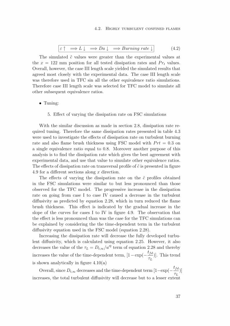
4.2. Highly turbulent confined flames
ε ↑ =⇒ L ↓ =⇒ Da ↓ =⇒ Burning rate ↓ (4.2)
The simulated c values were greater than the experimental values atthe x = 122 mm position for all tested dissipation rates and Prt values.Overall, however, the case III length scale yielded the simulated results thatagreed most closely with the experimental data. The case III length scalewas therefore used in TFC sin all the other equivalence ratio simulations.Therefore case III length scale was selected for TFC model to simulate allother subsequent equivalence ratios.
• Tuning:
5. Effect of varying the dissipation rate on FSC simulations
With the similar discussion as made in section 2.8, dissipation rate re-quired tuning. Therefore the same dissipation rates presented in table 4.3were used to investigate the effects of dissipation rate on turbulent burningrate and also flame brush thickness using FSC model with Prt = 0.3 ona single equivalence ratio equal to 0.8. Moreover another purpose of thisanalysis is to find the dissipation rate which gives the best agreement withexperimental data, and use that value to simulate other equivalence ratios.The effects of dissipation rate on transversal profile of c is presented in figure4.9 for a different sections along x direction.
The effects of varying the dissipation rate on the c profiles obtainedin the FSC simulations were similar to but less pronounced than thoseobserved for the TFC model. The progressive increase in the dissipationrate on going from case I to case IV caused a decrease in the turbulentdiffusivity as predicted by equation 2.28, which in turn reduced the flamebrush thickness. This effect is indicated by the gradual increase in theslope of the curves for cases I to IV in figure 4.9. The observation thatthe effect is less pronounced than was the case for the TFC simulations canbe explained by considering the the time-dependent term in the turbulentdiffusivity equation used in the FSC model (equation 2.28).
Increasing the dissipation rate will decrease the fully developed turbu-lent diffusivity, which is calculated using equation 2.25. However, it alsodecreases the value of the τL = Dt,∞/u′2 term of equation 2.28 and thereby
increases the value of the time-dependent term, [1−exp(−tfd
τL
)]. This trend
is shown analytically in figure 4.10(a)
Overall, since Dt,∞ decreases and the time-dependent term [1−exp(−tfd
τL
)]
increases, the total turbulent diffusivity will decrease but to a lesser extent
37
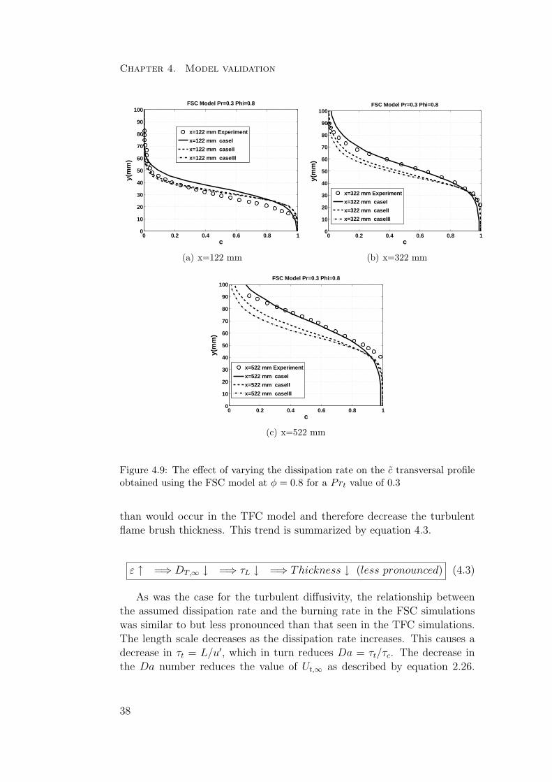
Chapter 4. Model validation
0 0.2 0.4 0.6 0.8 10
10
20
30
40
50
60
70
80
90
100
c
y(m
m)
FSC Model Pr=0.3 Phi=0.8
x=122 mm Experiment
x=122 mm caseI
x=122 mm caseII
x=122 mm caseIII
(a) x=122 mm
0 0.2 0.4 0.6 0.8 10
10
20
30
40
50
60
70
80
90
100
c
y(m
m)
FSC Model Pr=0.3 Phi=0.8
x=322 mm Experiment
x=322 mm caseI
x=322 mm caseII
x=322 mm caseIII
(b) x=322 mm
0 0.2 0.4 0.6 0.8 10
10
20
30
40
50
60
70
80
90
100
c
y(m
m)
FSC Model Pr=0.3 Phi=0.8
x=522 mm Experiment
x=522 mm caseI
x=522 mm caseII
x=522 mm caseIII
(c) x=522 mm
Figure 4.9: The effect of varying the dissipation rate on the c transversal profileobtained using the FSC model at φ = 0.8 for a Prt value of 0.3
than would occur in the TFC model and therefore decrease the turbulentflame brush thickness. This trend is summarized by equation 4.3.
ε ↑ =⇒ DT,∞ ↓ =⇒ τL ↓ =⇒ Thickness ↓ (less pronounced) (4.3)
As was the case for the turbulent diffusivity, the relationship betweenthe assumed dissipation rate and the burning rate in the FSC simulationswas similar to but less pronounced than that seen in the TFC simulations.The length scale decreases as the dissipation rate increases. This causes adecrease in τt = L/u′, which in turn reduces Da = τt/τc. The decrease inthe Da number reduces the value of Ut,∞ as described by equation 2.26.
38
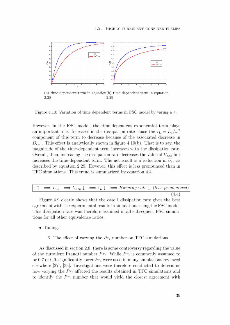
4.2. Highly turbulent confined flames
0 1 2 3 4 5 6 70
0.1
0.2
0.3
0.4
0.5
0.6
0.7
0.8
0.9
1
Dtt
t
τL,1
τL,2
> τL,1
(a) time dependent term in equation2.28
0 1 2 3 4 5 6 70
0.1
0.2
0.3
0.4
0.5
0.6
0.7
0.8
0.9
1
Utt
t
τL,1
τL,2
> τL,1
(b) time dependent term in equation2.29
Figure 4.10: Variation of time dependent terms in FSC model by varing a τL
However, in the FSC model, the time-dependent exponential term playsan important role. Increases in the dissipation rate cause the τL = Dt/u
′2
component of this term to decrease because of the associated decrease inDt,∞. This effect is analytically shown in figure 4.10(b). That is to say, themagnitude of the time-dependent term increases with the dissipation rate.Overall, then, increasing the dissipation rate decreases the value of Ut,∞ butincreases the time-dependent term. The net result is a reduction in Ut,t asdescribed by equation 2.29. However, this effect is less pronounced than inTFC simulations. This trend is summarized by equation 4.4.
ε ↑ =⇒ L ↓ =⇒ Ut,∞ ↓ =⇒ τL ↓ =⇒ Burning rate ↓ (less pronounced)
(4.4)Figure 4.9 clearly shows that the case I dissipation rate gives the best
agreement with the experimental results in simulations using the FSC model.This dissipation rate was therefore assumed in all subsequent FSC simula-tions for all other equivalence ratios.
• Tuning:
6. The effect of varying the Prt number on TFC simulations
As discussed in section 2.8, there is some controversy regarding the valueof the turbulent Prandtl number Prt. While Prt is commonly assumed tobe 0.7 or 0.9, significantly lower Prt were used in many simulations reviewedelsewhere [27], [33]. Investigations were therefore conducted to determinehow varying the Prt affected the results obtained in TFC simulations andto identify the Prt number that would yield the closest agreement with
39
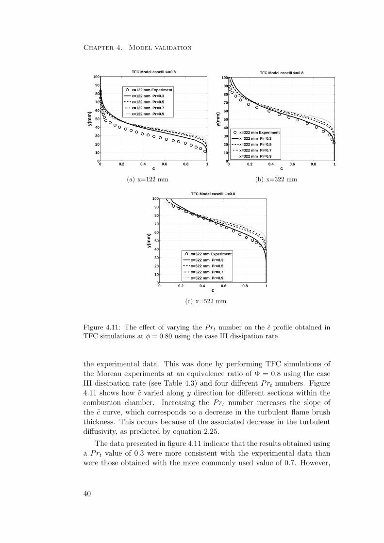
Chapter 4. Model validation
0 0.2 0.4 0.6 0.8 10
10
20
30
40
50
60
70
80
90
100
c
y(m
m)
TFC Model caseIII Φ=0.8
x=122 mm Experiment
x=122 mm Pr=0.3
x=122 mm Pr=0.5
x=122 mm Pr=0.7
x=122 mm Pr=0.9
(a) x=122 mm
0 0.2 0.4 0.6 0.8 10
10
20
30
40
50
60
70
80
90
100
c
y(m
m)
TFC Model caseIII Φ=0.8
x=322 mm Experiment
x=322 mm Pr=0.3
x=322 mm Pr=0.5
x=322 mm Pr=0.7
x=322 mm Pr=0.9
(b) x=322 mm
0 0.2 0.4 0.6 0.8 10
10
20
30
40
50
60
70
80
90
100
c
y(m
m)
TFC Model caseIII Φ=0.8
x=522 mm Experiment
x=522 mm Pr=0.3
x=522 mm Pr=0.5
x=522 mm Pr=0.7
x=522 mm Pr=0.9
(c) x=522 mm
Figure 4.11: The effect of varying the Prt number on the c profile obtained inTFC simulations at φ = 0.80 using the case III dissipation rate
the experimental data. This was done by performing TFC simulations ofthe Moreau experiments at an equivalence ratio of Φ = 0.8 using the caseIII dissipation rate (see Table 4.3) and four different Prt numbers. Figure4.11 shows how c varied along y direction for different sections within thecombustion chamber. Increasing the Prt number increases the slope ofthe c curve, which corresponds to a decrease in the turbulent flame brushthickness. This occurs because of the associated decrease in the turbulentdiffusivity, as predicted by equation 2.25.
The data presented in figure 4.11 indicate that the results obtained usinga Prt value of 0.3 were more consistent with the experimental data thanwere those obtained with the more commonly used value of 0.7. However,
40
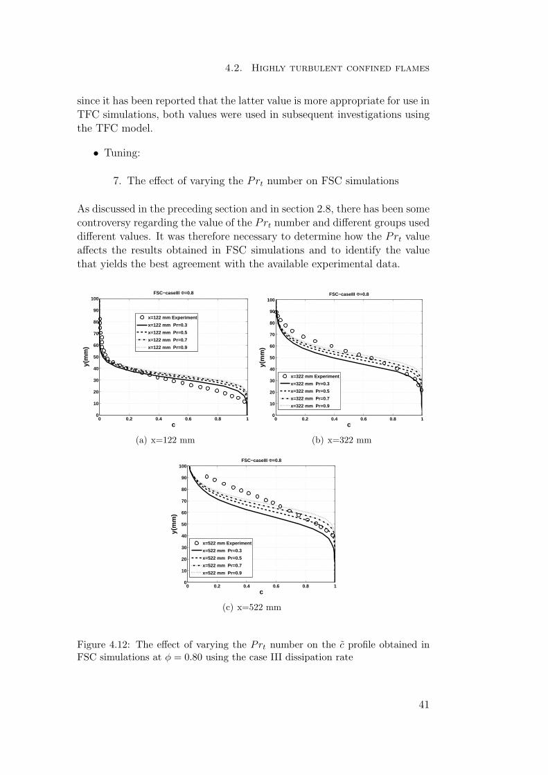
4.2. Highly turbulent confined flames
since it has been reported that the latter value is more appropriate for use inTFC simulations, both values were used in subsequent investigations usingthe TFC model.
• Tuning:
7. The effect of varying the Prt number on FSC simulations
As discussed in the preceding section and in section 2.8, there has been somecontroversy regarding the value of the Prt number and different groups useddifferent values. It was therefore necessary to determine how the Prt valueaffects the results obtained in FSC simulations and to identify the valuethat yields the best agreement with the available experimental data.
0 0.2 0.4 0.6 0.8 10
10
20
30
40
50
60
70
80
90
100
c
y(m
m)
FSC−caseIII Φ=0.8
x=122 mm Experiment
x=122 mm Pr=0.3
x=122 mm Pr=0.5
x=122 mm Pr=0.7
x=122 mm Pr=0.9
(a) x=122 mm
0 0.2 0.4 0.6 0.8 10
10
20
30
40
50
60
70
80
90
100
c
y(m
m)
FSC−caseIII Φ=0.8
x=322 mm Experiment
x=322 mm Pr=0.3
x=322 mm Pr=0.5
x=322 mm Pr=0.7
x=322 mm Pr=0.9
(b) x=322 mm
0 0.2 0.4 0.6 0.8 10
10
20
30
40
50
60
70
80
90
100
c
y(m
m)
FSC−caseIII Φ=0.8
x=522 mm Experiment
x=522 mm Pr=0.3
x=522 mm Pr=0.5
x=522 mm Pr=0.7
x=522 mm Pr=0.9
(c) x=522 mm
Figure 4.12: The effect of varying the Prt number on the c profile obtained inFSC simulations at φ = 0.80 using the case III dissipation rate
41
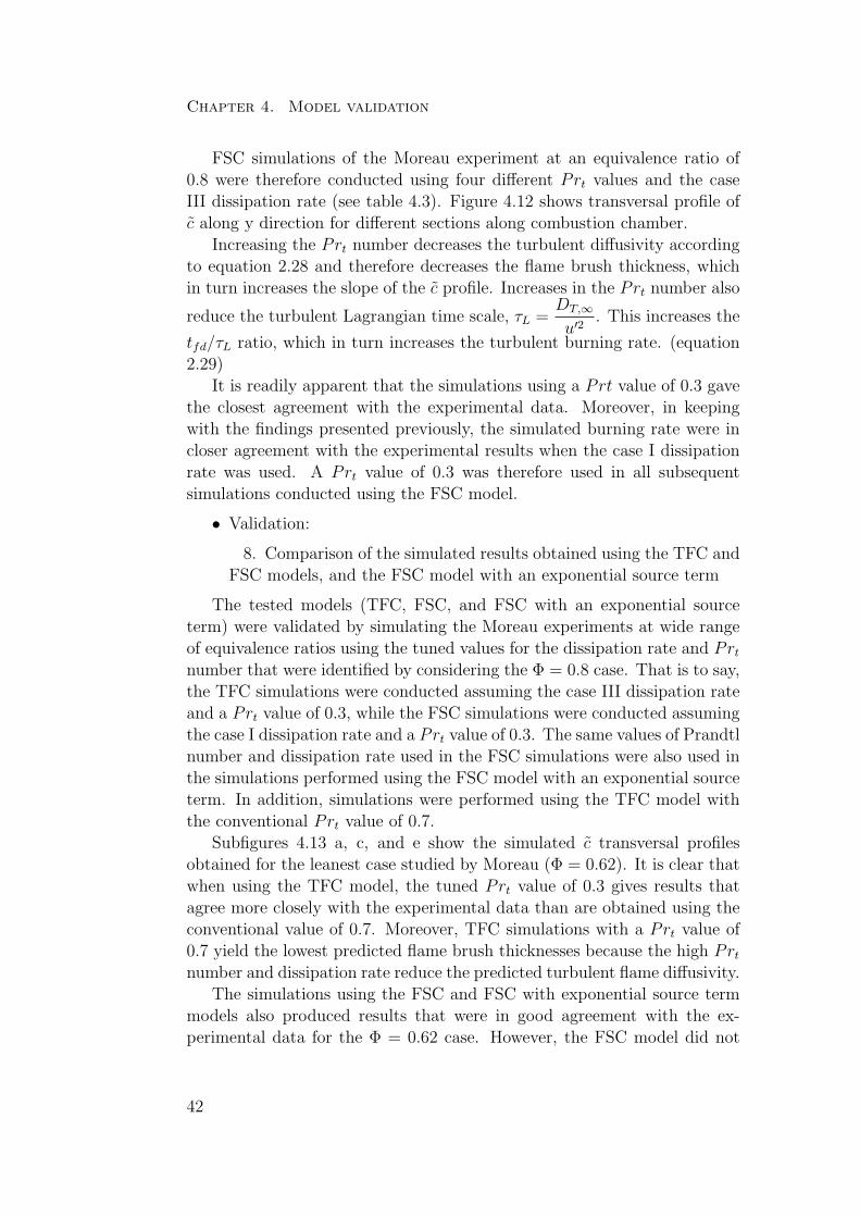
Chapter 4. Model validation
FSC simulations of the Moreau experiment at an equivalence ratio of0.8 were therefore conducted using four different Prt values and the caseIII dissipation rate (see table 4.3). Figure 4.12 shows transversal profile ofc along y direction for different sections along combustion chamber.
Increasing the Prt number decreases the turbulent diffusivity accordingto equation 2.28 and therefore decreases the flame brush thickness, whichin turn increases the slope of the c profile. Increases in the Prt number also
reduce the turbulent Lagrangian time scale, τL =DT,∞
u′2. This increases the
tfd/τL ratio, which in turn increases the turbulent burning rate. (equation2.29)
It is readily apparent that the simulations using a Prt value of 0.3 gavethe closest agreement with the experimental data. Moreover, in keepingwith the findings presented previously, the simulated burning rate were incloser agreement with the experimental results when the case I dissipationrate was used. A Prt value of 0.3 was therefore used in all subsequentsimulations conducted using the FSC model.
• Validation:
8. Comparison of the simulated results obtained using the TFC andFSC models, and the FSC model with an exponential source term
The tested models (TFC, FSC, and FSC with an exponential sourceterm) were validated by simulating the Moreau experiments at wide rangeof equivalence ratios using the tuned values for the dissipation rate and Prt
number that were identified by considering the Φ = 0.8 case. That is to say,the TFC simulations were conducted assuming the case III dissipation rateand a Prt value of 0.3, while the FSC simulations were conducted assumingthe case I dissipation rate and a Prt value of 0.3. The same values of Prandtlnumber and dissipation rate used in the FSC simulations were also used inthe simulations performed using the FSC model with an exponential sourceterm. In addition, simulations were performed using the TFC model withthe conventional Prt value of 0.7.
Subfigures 4.13 a, c, and e show the simulated c transversal profilesobtained for the leanest case studied by Moreau (Φ = 0.62). It is clear thatwhen using the TFC model, the tuned Prt value of 0.3 gives results thatagree more closely with the experimental data than are obtained using theconventional value of 0.7. Moreover, TFC simulations with a Prt value of0.7 yield the lowest predicted flame brush thicknesses because the high Prt
number and dissipation rate reduce the predicted turbulent flame diffusivity.The simulations using the FSC and FSC with exponential source term
models also produced results that were in good agreement with the ex-perimental data for the Φ = 0.62 case. However, the FSC model did not
42
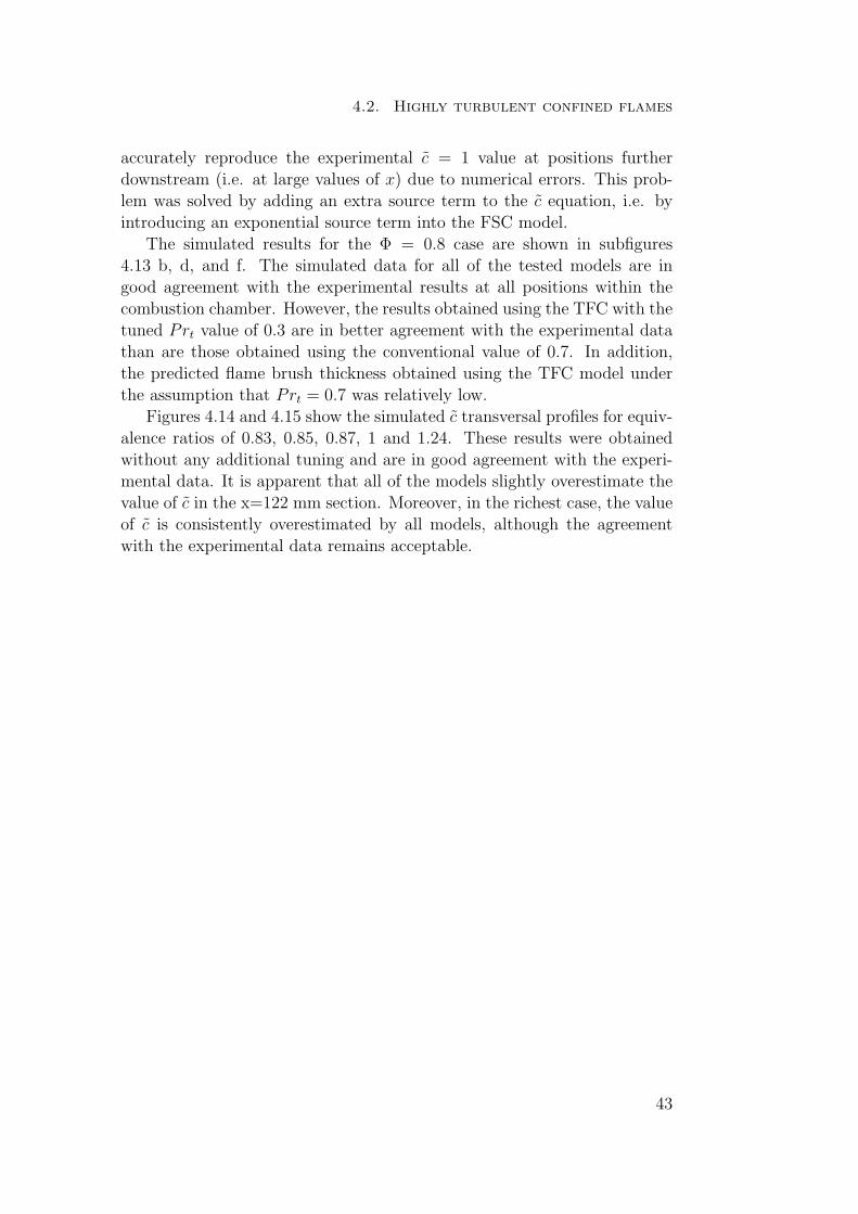
4.2. Highly turbulent confined flames
accurately reproduce the experimental c = 1 value at positions furtherdownstream (i.e. at large values of x) due to numerical errors. This prob-lem was solved by adding an extra source term to the c equation, i.e. byintroducing an exponential source term into the FSC model.
The simulated results for the Φ = 0.8 case are shown in subfigures4.13 b, d, and f. The simulated data for all of the tested models are ingood agreement with the experimental results at all positions within thecombustion chamber. However, the results obtained using the TFC with thetuned Prt value of 0.3 are in better agreement with the experimental datathan are those obtained using the conventional value of 0.7. In addition,the predicted flame brush thickness obtained using the TFC model underthe assumption that Prt = 0.7 was relatively low.
Figures 4.14 and 4.15 show the simulated c transversal profiles for equiv-alence ratios of 0.83, 0.85, 0.87, 1 and 1.24. These results were obtainedwithout any additional tuning and are in good agreement with the experi-mental data. It is apparent that all of the models slightly overestimate thevalue of c in the x=122 mm section. Moreover, in the richest case, the valueof c is consistently overestimated by all models, although the agreementwith the experimental data remains acceptable.
43
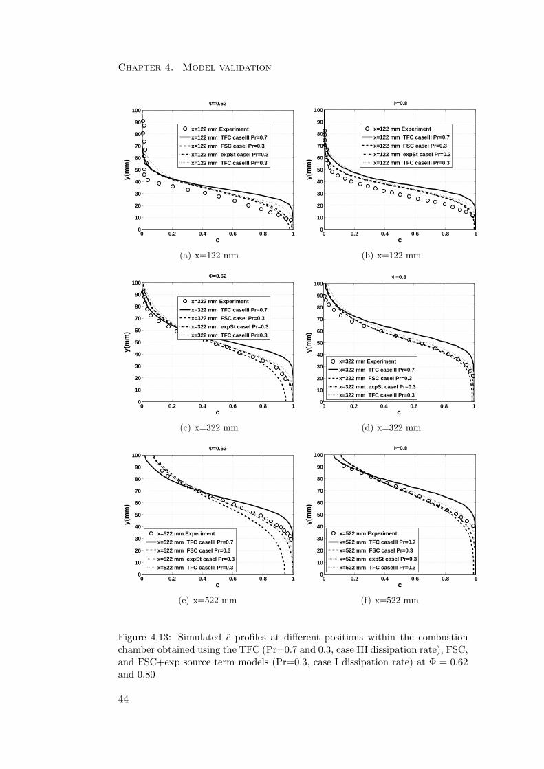
Chapter 4. Model validation
0 0.2 0.4 0.6 0.8 10
10
20
30
40
50
60
70
80
90
100
c
y(m
m)
Φ=0.62
x=122 mm Experiment
x=122 mm TFC caseIII Pr=0.7
x=122 mm FSC caseI Pr=0.3
x=122 mm expSt caseI Pr=0.3
x=122 mm TFC caseIII Pr=0.3
(a) x=122 mm
0 0.2 0.4 0.6 0.8 10
10
20
30
40
50
60
70
80
90
100
c
y(m
m)
Φ=0.8
x=122 mm Experiment
x=122 mm TFC caseIII Pr=0.7
x=122 mm FSC caseI Pr=0.3
x=122 mm expSt caseI Pr=0.3
x=122 mm TFC caseIII Pr=0.3
(b) x=122 mm
0 0.2 0.4 0.6 0.8 10
10
20
30
40
50
60
70
80
90
100
c
y(m
m)
Φ=0.62
x=322 mm Experiment
x=322 mm TFC caseIII Pr=0.7
x=322 mm FSC caseI Pr=0.3
x=322 mm expSt caseI Pr=0.3
x=322 mm TFC caseIII Pr=0.3
(c) x=322 mm
0 0.2 0.4 0.6 0.8 10
10
20
30
40
50
60
70
80
90
100
c
y(m
m)
Φ=0.8
x=322 mm Experiment
x=322 mm TFC caseIII Pr=0.7
x=322 mm FSC caseI Pr=0.3
x=322 mm expSt caseI Pr=0.3
x=322 mm TFC caseIII Pr=0.3
(d) x=322 mm
0 0.2 0.4 0.6 0.8 10
10
20
30
40
50
60
70
80
90
100
c
y(m
m)
Φ=0.62
x=522 mm Experiment
x=522 mm TFC caseIII Pr=0.7
x=522 mm FSC caseI Pr=0.3
x=522 mm expSt caseI Pr=0.3
x=522 mm TFC caseIII Pr=0.3
(e) x=522 mm
0 0.2 0.4 0.6 0.8 10
10
20
30
40
50
60
70
80
90
100
c
y(m
m)
Φ=0.8
x=522 mm Experiment
x=522 mm TFC caseIII Pr=0.7
x=522 mm FSC caseI Pr=0.3
x=522 mm expSt caseI Pr=0.3
x=522 mm TFC caseIII Pr=0.3
(f) x=522 mm
Figure 4.13: Simulated c profiles at different positions within the combustionchamber obtained using the TFC (Pr=0.7 and 0.3, case III dissipation rate), FSC,and FSC+exp source term models (Pr=0.3, case I dissipation rate) at Φ = 0.62and 0.80
44
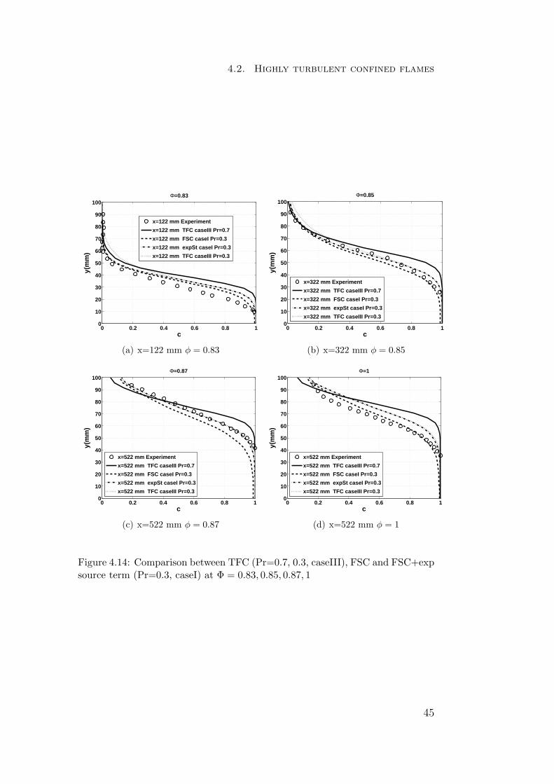
4.2. Highly turbulent confined flames
0 0.2 0.4 0.6 0.8 10
10
20
30
40
50
60
70
80
90
100
c
y(m
m)
Φ=0.83
x=122 mm Experiment
x=122 mm TFC caseIII Pr=0.7
x=122 mm FSC caseI Pr=0.3
x=122 mm expSt caseI Pr=0.3
x=122 mm TFC caseIII Pr=0.3
(a) x=122 mm φ = 0.83
0 0.2 0.4 0.6 0.8 10
10
20
30
40
50
60
70
80
90
100
c
y(m
m)
Φ=0.85
x=322 mm Experiment
x=322 mm TFC caseIII Pr=0.7
x=322 mm FSC caseI Pr=0.3
x=322 mm expSt caseI Pr=0.3
x=322 mm TFC caseIII Pr=0.3
(b) x=322 mm φ = 0.85
0 0.2 0.4 0.6 0.8 10
10
20
30
40
50
60
70
80
90
100
c
y(m
m)
Φ=0.87
x=522 mm Experiment
x=522 mm TFC caseIII Pr=0.7
x=522 mm FSC caseI Pr=0.3
x=522 mm expSt caseI Pr=0.3
x=522 mm TFC caseIII Pr=0.3
(c) x=522 mm φ = 0.87
0 0.2 0.4 0.6 0.8 10
10
20
30
40
50
60
70
80
90
100
c
y(m
m)
Φ=1
x=522 mm Experiment
x=522 mm TFC caseIII Pr=0.7
x=522 mm FSC caseI Pr=0.3
x=522 mm expSt caseI Pr=0.3
x=522 mm TFC caseIII Pr=0.3
(d) x=522 mm φ = 1
Figure 4.14: Comparison between TFC (Pr=0.7, 0.3, caseIII), FSC and FSC+expsource term (Pr=0.3, caseI) at Φ = 0.83, 0.85, 0.87, 1
45
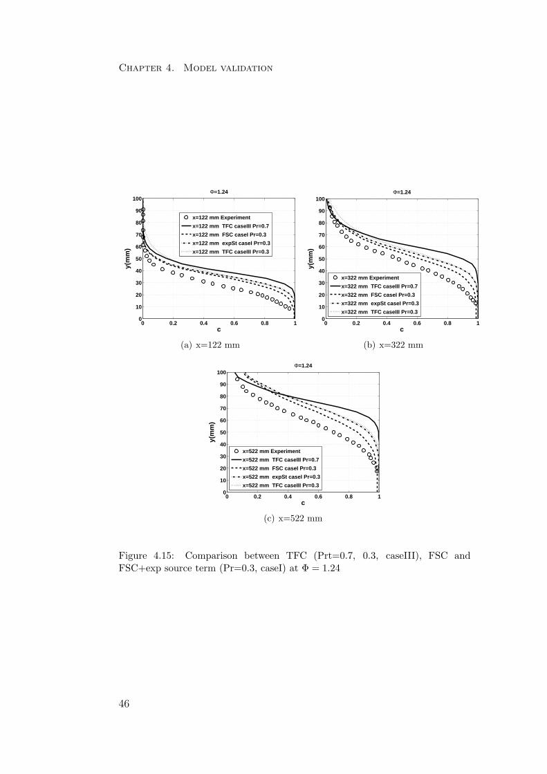
Chapter 4. Model validation
0 0.2 0.4 0.6 0.8 10
10
20
30
40
50
60
70
80
90
100
c
y(m
m)
Φ=1.24
x=122 mm Experiment
x=122 mm TFC caseIII Pr=0.7
x=122 mm FSC caseI Pr=0.3
x=122 mm expSt caseI Pr=0.3
x=122 mm TFC caseIII Pr=0.3
(a) x=122 mm
0 0.2 0.4 0.6 0.8 10
10
20
30
40
50
60
70
80
90
100
c
y(m
m)
Φ=1.24
x=322 mm Experiment
x=322 mm TFC caseIII Pr=0.7
x=322 mm FSC caseI Pr=0.3
x=322 mm expSt caseI Pr=0.3
x=322 mm TFC caseIII Pr=0.3
(b) x=322 mm
0 0.2 0.4 0.6 0.8 10
10
20
30
40
50
60
70
80
90
100
c
y(m
m)
Φ=1.24
x=522 mm Experiment
x=522 mm TFC caseIII Pr=0.7
x=522 mm FSC caseI Pr=0.3
x=522 mm expSt caseI Pr=0.3
x=522 mm TFC caseIII Pr=0.3
(c) x=522 mm
Figure 4.15: Comparison between TFC (Prt=0.7, 0.3, caseIII), FSC andFSC+exp source term (Pr=0.3, caseI) at Φ = 1.24
46
4.2. Highly turbulent confined flames
4.2.4 Conclusion
The TFC and FSC models of premixed turbulent combustion were imple-mented in OpenFOAM and used to simulate the experiments reported byMoreau [1], who studied oblique preheated lean methane-air flames gen-erated from mixtures with different equivalence ratios (Φ=0.62-1.24) in ahighly intense turbulent flow with stabilization by a hot product flow inan adjacent channel. The values of two parameters used in these models- the dissipation rate and the turbulent Prandtl number - were tuned toreproduce the experimental results for a single equivalence ratio (Φ = 0.8).The resulting tuned values were then used without further modification tosimulate the experiments performed at other equivalence ratios. Compari-son of results computed using the two models, with all other things beingequal, indicates that premixed turbulent flame development plays a role byreducing the burning rate and mean flame brush thickness in the consideredcase. The reasonable agreement between the experimental and numericaldata shows that both models are capable of reproducing experimental re-sults with at least some level of accuracy but cannot be taken as a completevalidation of their predictive capabilities because the results obtained weresensitive to the inflow boundary condition for the mean dissipation rate.However, this sensitivity was less pronounced for the FSC model.
47
Chapter 4. Model validation
4.3 V-shape flames
4.3.1 The simulated test case
The second experimental study that was used as a source of reference datain this work was the examination of non-confined turbulent premixed V-shaped flames conducted by Dinkelacker and Holzler [2]. Figure 4.16(a)shows the experimental setup used by these authors. Their apparatus fea-tures a nozzle with a diameter of 40 mm and a perforated plate that islocated 70 mm beneath the nozzle’s aperture. In addition, there is a 2 mmstabilizer wire located 10 mm above the nozzle exit. These experiments areattractive as sources of reference data for numerical simulations because ofthe simple geometric configuration of the flow and the homogeneous tur-bulence created by using a perforated plate. Moreover, the mean flamelocation in this system can be specified in terms of the flame angle, whichis a useful parameter when comparing simulated and experimental data.Several groups have therefore conducted modeling studies based on theseexperiments:
i) Dinkelacker and Holzler [2] conducted studies using the TFC modeland two other models with different expressions for the reaction rateii) Ghirelli [37] performed investigations using the original TFC model anda modified variant that is based on Ghirelli’s dispersion model [38].iii) Moreau [46] [47] studied the Dinkelacker and Holzler system using theoriginal TFC model and a modified variant known as the self-similar tur-bulent flame (SSTF) model
However, the FSC model has not yet been used to simulate these exper-iments.
4.3.2 Numerical setup and sensitivity analysis
Simulations were performed for all three of the equivalence ratios exam-ined by Dinkelacker and Holzler (Φ = 0.5, Φ = 0.58, Φ = 0.7) and withthe mean inlet velocity equal to 3.04 m/s. Simulations performed usingthe TFC (equations 2.24 and 2.26) and FSC (equations 2.30 2.28 and 2.29)models. The standard k-ε model [39] was used to simulate the turbulence ineach case. Two additional sets of simulations were conducted to investigatethe effect of compressibility in this system, since it is known to be impor-tant in engines. The first set was conducted using the FSC model with thestandard k-ε model (c3 = 0), while the second set used the FSC model inconjunction with the extended k-ε model (c3 = −0.33, see equation 2.36).The progress variable fields for these two cases are shown in figure 4.17
48
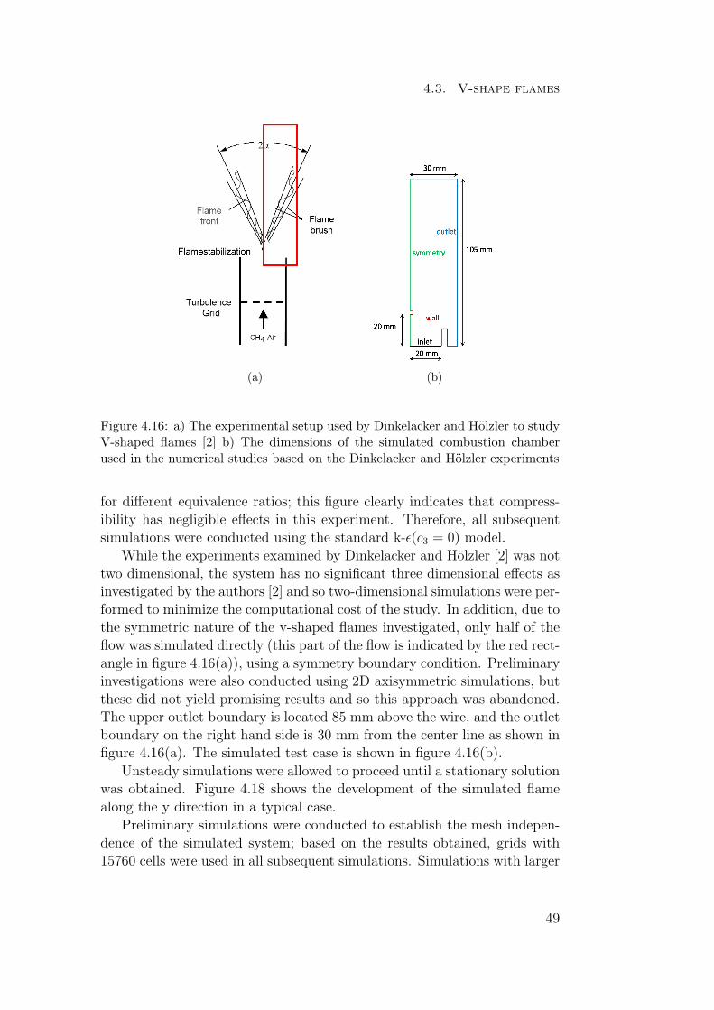
4.3. V-shape flames
(a) (b)
Figure 4.16: a) The experimental setup used by Dinkelacker and Holzler to studyV-shaped flames [2] b) The dimensions of the simulated combustion chamberused in the numerical studies based on the Dinkelacker and Holzler experiments
for different equivalence ratios; this figure clearly indicates that compress-ibility has negligible effects in this experiment. Therefore, all subsequentsimulations were conducted using the standard k-ǫ(c3 = 0) model.
While the experiments examined by Dinkelacker and Holzler [2] was nottwo dimensional, the system has no significant three dimensional effects asinvestigated by the authors [2] and so two-dimensional simulations were per-formed to minimize the computational cost of the study. In addition, due tothe symmetric nature of the v-shaped flames investigated, only half of theflow was simulated directly (this part of the flow is indicated by the red rect-angle in figure 4.16(a)), using a symmetry boundary condition. Preliminaryinvestigations were also conducted using 2D axisymmetric simulations, butthese did not yield promising results and so this approach was abandoned.The upper outlet boundary is located 85 mm above the wire, and the outletboundary on the right hand side is 30 mm from the center line as shown infigure 4.16(a). The simulated test case is shown in figure 4.16(b).
Unsteady simulations were allowed to proceed until a stationary solutionwas obtained. Figure 4.18 shows the development of the simulated flamealong the y direction in a typical case.
Preliminary simulations were conducted to establish the mesh indepen-dence of the simulated system; based on the results obtained, grids with15760 cells were used in all subsequent simulations. Simulations with larger
49
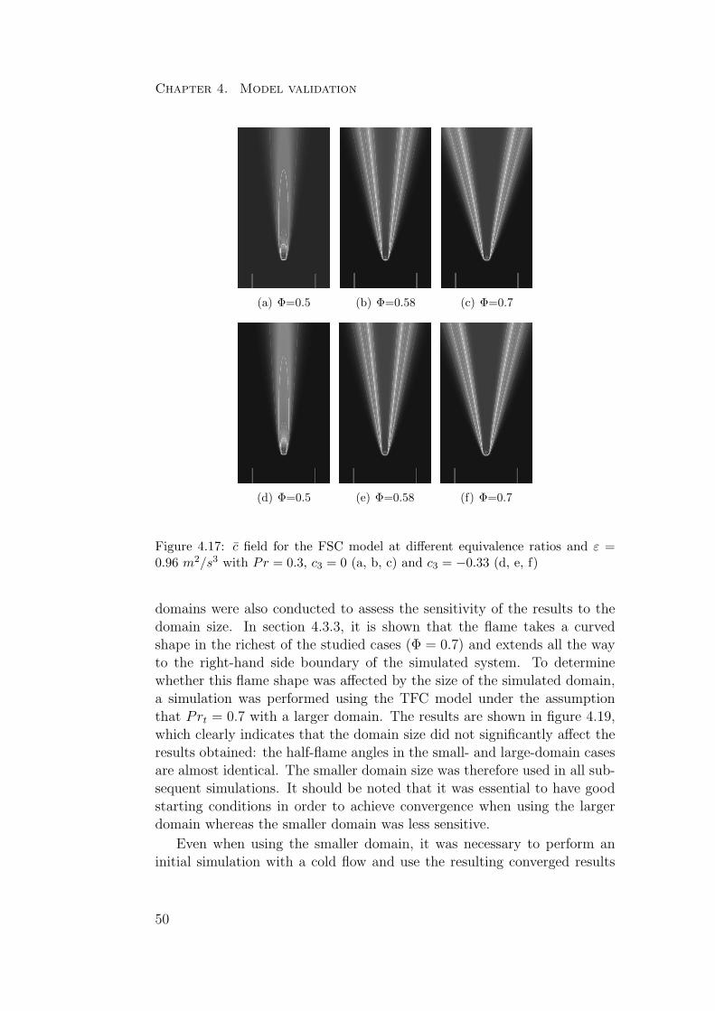
Chapter 4. Model validation
(a) Φ=0.5 (b) Φ=0.58 (c) Φ=0.7
(d) Φ=0.5 (e) Φ=0.58 (f) Φ=0.7
Figure 4.17: c field for the FSC model at different equivalence ratios and ε =0.96 m2/s3 with Pr = 0.3, c3 = 0 (a, b, c) and c3 = −0.33 (d, e, f)
domains were also conducted to assess the sensitivity of the results to thedomain size. In section 4.3.3, it is shown that the flame takes a curvedshape in the richest of the studied cases (Φ = 0.7) and extends all the wayto the right-hand side boundary of the simulated system. To determinewhether this flame shape was affected by the size of the simulated domain,a simulation was performed using the TFC model under the assumptionthat Prt = 0.7 with a larger domain. The results are shown in figure 4.19,which clearly indicates that the domain size did not significantly affect theresults obtained: the half-flame angles in the small- and large-domain casesare almost identical. The smaller domain size was therefore used in all sub-sequent simulations. It should be noted that it was essential to have goodstarting conditions in order to achieve convergence when using the largerdomain whereas the smaller domain was less sensitive.
Even when using the smaller domain, it was necessary to perform aninitial simulation with a cold flow and use the resulting converged results
50
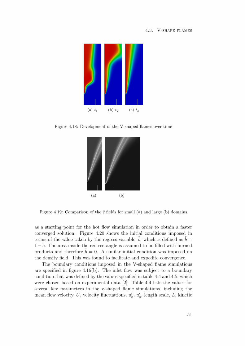
4.3. V-shape flames
(a) t1 (b) t2 (c) t3
Figure 4.18: Development of the V-shaped flames over time
(a) (b)
Figure 4.19: Comparison of the c fields for small (a) and large (b) domains
as a starting point for the hot flow simulation in order to obtain a fasterconverged solution. Figure 4.20 shows the initial conditions imposed interms of the value taken by the regress variable, b, which is defined as b =1− c. The area inside the red rectangle is assumed to be filled with burnedproducts and therefore b = 0. A similar initial condition was imposed onthe density field. This was found to facilitate and expedite convergence.
The boundary conditions imposed in the V-shaped flame simulationsare specified in figure 4.16(b). The inlet flow was subject to a boundarycondition that was defined by the values specified in table 4.4 and 4.5, whichwere chosen based on experimental data [2]. Table 4.4 lists the values forseveral key parameters in the v-shaped flame simulations, including themean flow velocity, U , velocity fluctuations, u′
x, u′y, length scale, L, kinetic
51
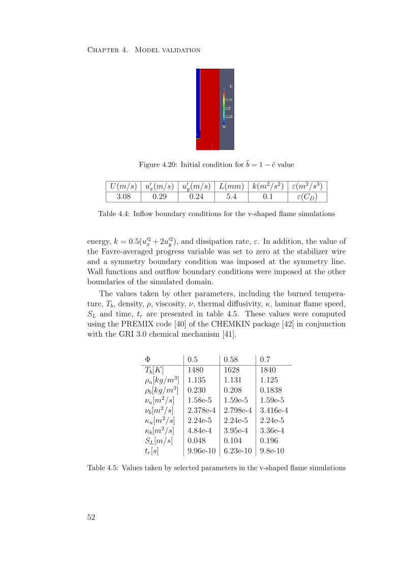
Chapter 4. Model validation
Figure 4.20: Initial condition for b = 1 − c value
U(m/s) u′x(m/s) u′
y(m/s) L(mm) k(m2/s2) ε(m2/s3)
3.08 0.29 0.24 5.4 0.1 ε(CD)
Table 4.4: Inflow boundary conditions for the v-shaped flame simulations
energy, k = 0.5(u′2x +2u′2
y ), and dissipation rate, ε. In addition, the value ofthe Favre-averaged progress variable was set to zero at the stabilizer wireand a symmetry boundary condition was imposed at the symmetry line.Wall functions and outflow boundary conditions were imposed at the otherboundaries of the simulated domain.
The values taken by other parameters, including the burned tempera-ture, Tb, density, ρ, viscosity, ν, thermal diffusivity, κ, laminar flame speed,SL and time, tr are presented in table 4.5. These values were computedusing the PREMIX code [40] of the CHEMKIN package [42] in conjunctionwith the GRI 3.0 chemical mechanism [41].
Φ 0.5 0.58 0.7
Tb[K] 1480 1628 1840ρu[kg/m3] 1.135 1.131 1.125ρb[kg/m3] 0.230 0.208 0.1838νu[m
2/s] 1.58e-5 1.59e-5 1.59e-5νb[m
2/s] 2.378e-4 2.798e-4 3.416e-4κu[m
2/s] 2.24e-5 2.24e-5 2.24e-5κb[m
2/s] 4.84e-4 3.95e-4 3.36e-4SL[m/s] 0.048 0.104 0.196tr[s] 9.96e-10 6.23e-10 9.8e-10
Table 4.5: Values taken by selected parameters in the v-shaped flame simulations
52
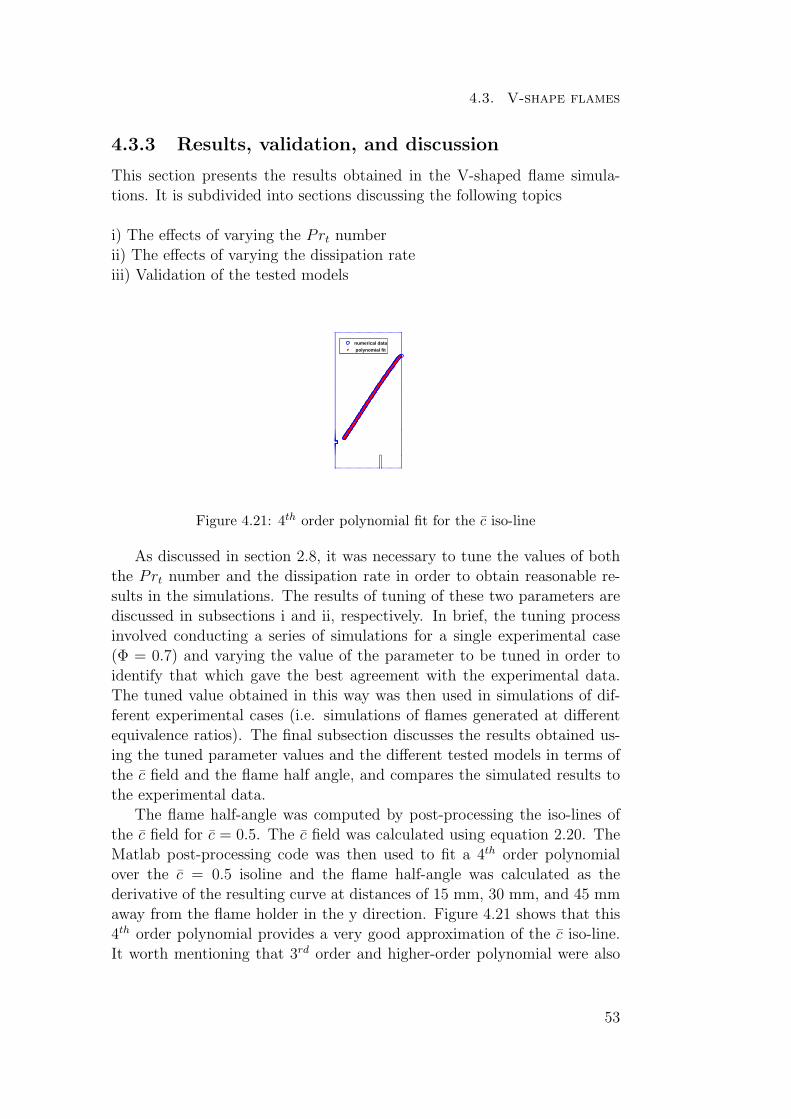
4.3. V-shape flames
4.3.3 Results, validation, and discussion
This section presents the results obtained in the V-shaped flame simula-tions. It is subdivided into sections discussing the following topics
i) The effects of varying the Prt numberii) The effects of varying the dissipation rateiii) Validation of the tested models
numerical data polynomial fit
Figure 4.21: 4th order polynomial fit for the c iso-line
As discussed in section 2.8, it was necessary to tune the values of boththe Prt number and the dissipation rate in order to obtain reasonable re-sults in the simulations. The results of tuning of these two parameters arediscussed in subsections i and ii, respectively. In brief, the tuning processinvolved conducting a series of simulations for a single experimental case(Φ = 0.7) and varying the value of the parameter to be tuned in order toidentify that which gave the best agreement with the experimental data.The tuned value obtained in this way was then used in simulations of dif-ferent experimental cases (i.e. simulations of flames generated at differentequivalence ratios). The final subsection discusses the results obtained us-ing the tuned parameter values and the different tested models in terms ofthe c field and the flame half angle, and compares the simulated results tothe experimental data.
The flame half-angle was computed by post-processing the iso-lines ofthe c field for c = 0.5. The c field was calculated using equation 2.20. TheMatlab post-processing code was then used to fit a 4th order polynomialover the c = 0.5 isoline and the flame half-angle was calculated as thederivative of the resulting curve at distances of 15 mm, 30 mm, and 45 mmaway from the flame holder in the y direction. Figure 4.21 shows that this4th order polynomial provides a very good approximation of the c iso-line.It worth mentioning that 3rd order and higher-order polynomial were also
53
Chapter 4. Model validation
tested and yielded very similar flame angles to those obtained using the 4th
order polynomials.The results are presented in the following order:
• The effects of varying the Prt number
1. In FSC simulations assuming ε = 0.96 m2/s3
2. In FSC simulations using an exponential source term and assum-ing that ε = 0.96 or 4.80 m2/s3
• The effects of varying the dissipation rate
3. In TFC simulations assuming Prt = 0.7, Φ = 0.7
4. In FSC simulations using an exponential source term and assum-ing that Prt = 0.5
• Validation and Comparison
54
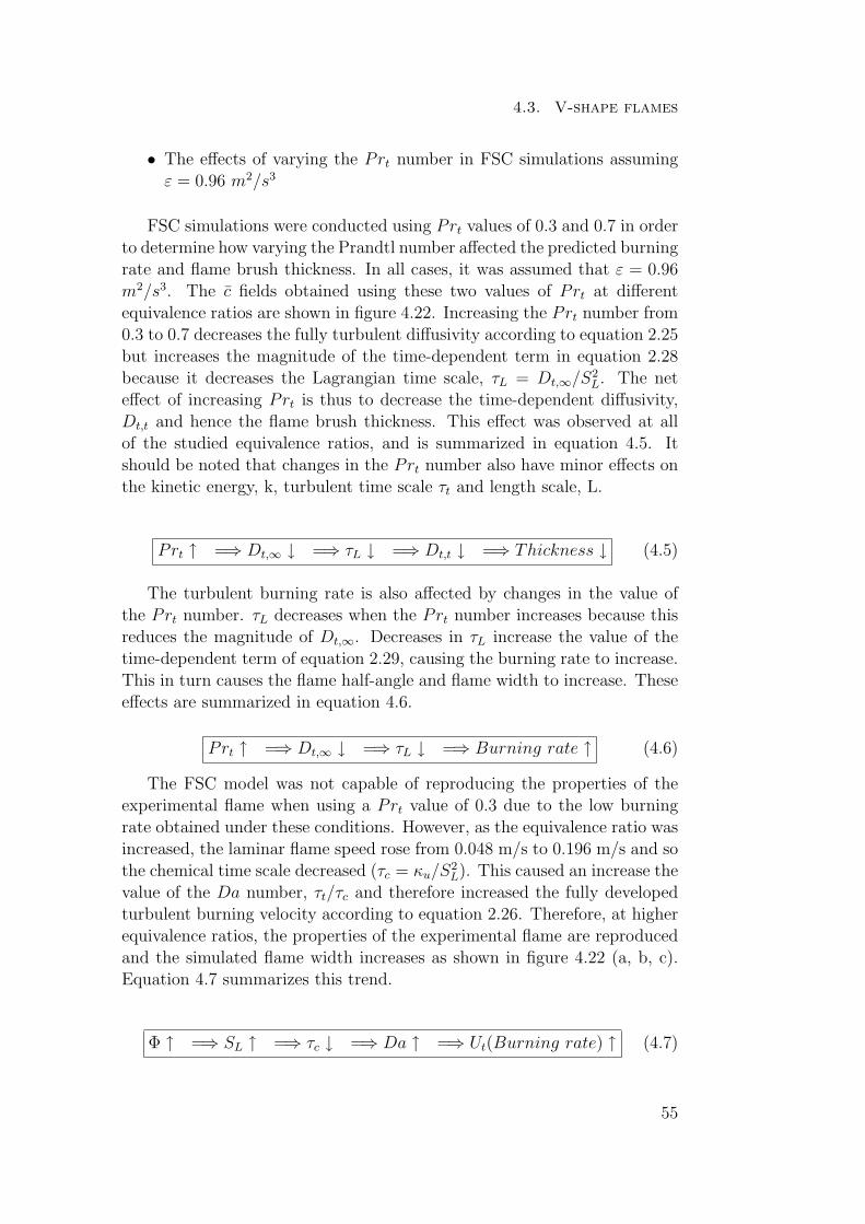
4.3. V-shape flames
• The effects of varying the Prt number in FSC simulations assumingε = 0.96 m2/s3
FSC simulations were conducted using Prt values of 0.3 and 0.7 in orderto determine how varying the Prandtl number affected the predicted burningrate and flame brush thickness. In all cases, it was assumed that ε = 0.96m2/s3. The c fields obtained using these two values of Prt at differentequivalence ratios are shown in figure 4.22. Increasing the Prt number from0.3 to 0.7 decreases the fully turbulent diffusivity according to equation 2.25but increases the magnitude of the time-dependent term in equation 2.28because it decreases the Lagrangian time scale, τL = Dt,∞/S2
L. The neteffect of increasing Prt is thus to decrease the time-dependent diffusivity,Dt,t and hence the flame brush thickness. This effect was observed at allof the studied equivalence ratios, and is summarized in equation 4.5. Itshould be noted that changes in the Prt number also have minor effects onthe kinetic energy, k, turbulent time scale τt and length scale, L.
Prt ↑ =⇒ Dt,∞ ↓ =⇒ τL ↓ =⇒ Dt,t ↓ =⇒ Thickness ↓ (4.5)
The turbulent burning rate is also affected by changes in the value ofthe Prt number. τL decreases when the Prt number increases because thisreduces the magnitude of Dt,∞. Decreases in τL increase the value of thetime-dependent term of equation 2.29, causing the burning rate to increase.This in turn causes the flame half-angle and flame width to increase. Theseeffects are summarized in equation 4.6.
Prt ↑ =⇒ Dt,∞ ↓ =⇒ τL ↓ =⇒ Burning rate ↑ (4.6)
The FSC model was not capable of reproducing the properties of theexperimental flame when using a Prt value of 0.3 due to the low burningrate obtained under these conditions. However, as the equivalence ratio wasincreased, the laminar flame speed rose from 0.048 m/s to 0.196 m/s and sothe chemical time scale decreased (τc = κu/S
2
L). This caused an increase thevalue of the Da number, τt/τc and therefore increased the fully developedturbulent burning velocity according to equation 2.26. Therefore, at higherequivalence ratios, the properties of the experimental flame are reproducedand the simulated flame width increases as shown in figure 4.22 (a, b, c).Equation 4.7 summarizes this trend.
Φ ↑ =⇒ SL ↑ =⇒ τc ↓ =⇒ Da ↑ =⇒ Ut(Burning rate) ↑ (4.7)
55
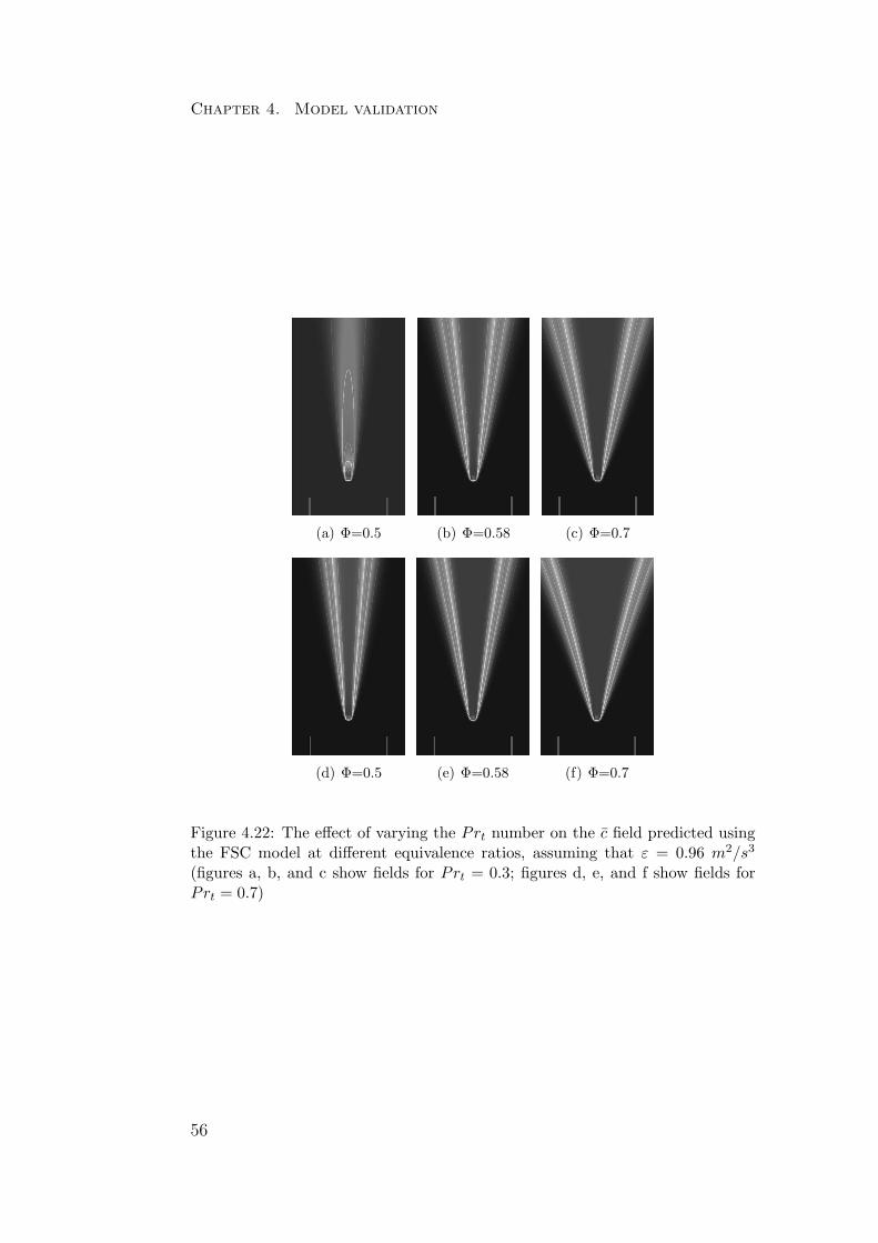
Chapter 4. Model validation
(a) Φ=0.5 (b) Φ=0.58 (c) Φ=0.7
(d) Φ=0.5 (e) Φ=0.58 (f) Φ=0.7
Figure 4.22: The effect of varying the Prt number on the c field predicted usingthe FSC model at different equivalence ratios, assuming that ε = 0.96 m2/s3
(figures a, b, and c show fields for Prt = 0.3; figures d, e, and f show fields forPrt = 0.7)
56
4.3. V-shape flames
The increases in the burning rate caused by increasing the Prt numberor the equivalence ratio are also readily apparent in figure 4.23, which showsplots of the flame half-angle against Φ for two different Prt numbers.
In the leanest case for which experimental data are available (Φ = 0.7),the simulations accurately reproduced the experimental results using a Prt
number of 0.7. However, to identify an optimal value of Prt for general use,additional simulations were conducted.
0.5 0.55 0.6 0.65 0.7 0.754
6
8
10
12
14
16
18
20
22
24
angl
e
Φ
simulation, Pr=0.3simulation, Pr=0.7experiment
Figure 4.23: The flame half-angle as a function of Φ for Prt = 0.3 and Prt = 0.7as predicted using the FSC model with ε = 0.96 m2/s3
The simulated results shown in figure 4.23 indicate that the FSC modelunderestimates the measured burning rate if the exponential source term isomitted. As shown in the next subsection, the inclusion of this source termcan be quite important when considering the weakly turbulent conditionsassociated with the studied flames.
• The effects of varying the Prt number in FSC simulations using anexponential source term and assuming ε = 0.96 m2/s3, Φ = 0.7
Simulations were performed using the FSC model with an exponentialsource term for five different Prt numbers (ranging from 0.3 to 0.7) at asingle equivalence ratio, Φ = 0.7, in order to identify the value that wouldyield the closest agreement with the experimental data. The effects of vary-ing the Prt number on the simulated flame brush thickness and turbulentburning rate were similar to those discussed in the previous subsection andsummarized in equations 4.6 and 4.5.
Figure 4.22 clearly shows that the inclusion of an extra source term inthe equation for c in these simulations produces a thinner predicted flamebrush than was obtained in its absence.
Variation of the Prt number can also affect the turbulent burning rate.As can be seen in figure 4.24, the turbulent burning rate increases in parallelwith Prt. That is to say, the flame width and the flame half-angle are
57
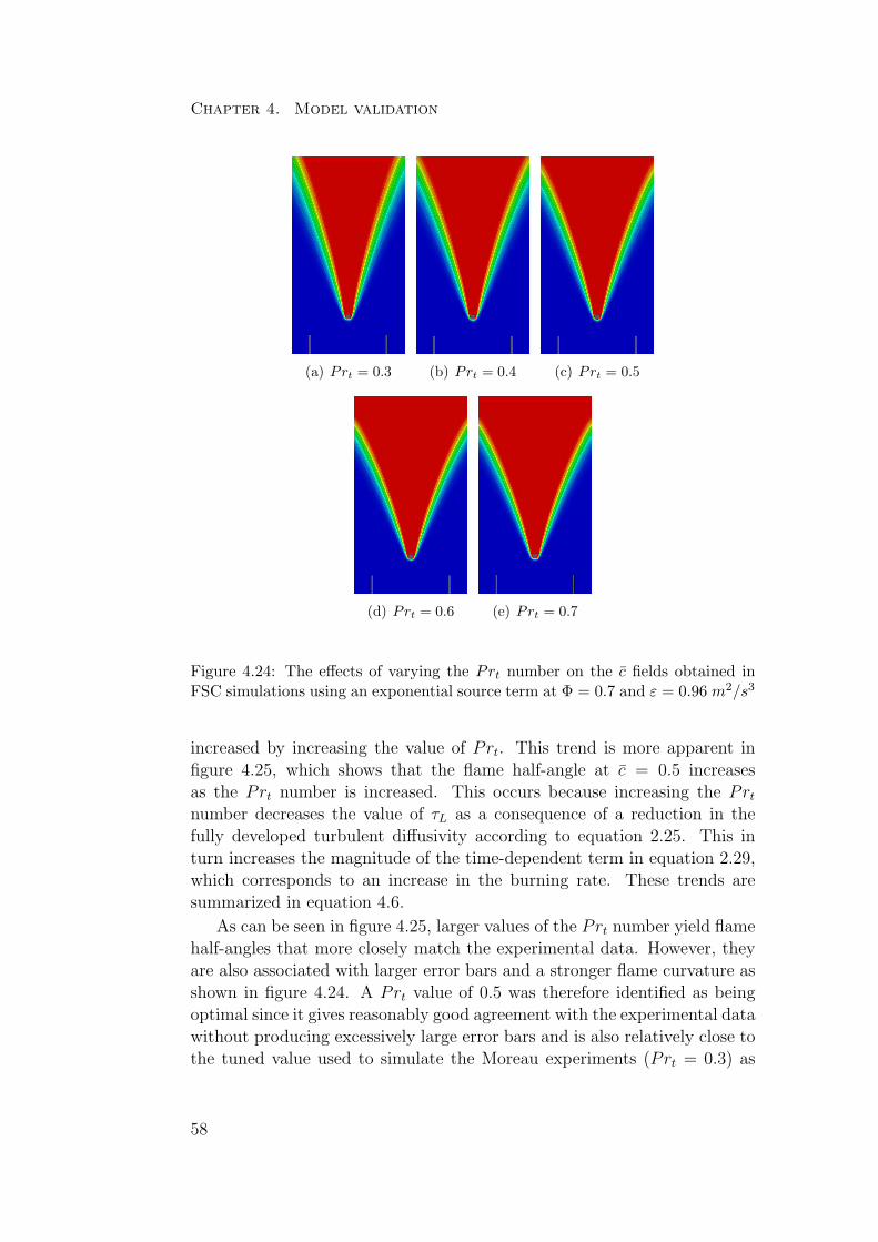
Chapter 4. Model validation
(a) Prt = 0.3 (b) Prt = 0.4 (c) Prt = 0.5
(d) Prt = 0.6 (e) Prt = 0.7
Figure 4.24: The effects of varying the Prt number on the c fields obtained inFSC simulations using an exponential source term at Φ = 0.7 and ε = 0.96 m2/s3
increased by increasing the value of Prt. This trend is more apparent infigure 4.25, which shows that the flame half-angle at c = 0.5 increasesas the Prt number is increased. This occurs because increasing the Prt
number decreases the value of τL as a consequence of a reduction in thefully developed turbulent diffusivity according to equation 2.25. This inturn increases the magnitude of the time-dependent term in equation 2.29,which corresponds to an increase in the burning rate. These trends aresummarized in equation 4.6.
As can be seen in figure 4.25, larger values of the Prt number yield flamehalf-angles that more closely match the experimental data. However, theyare also associated with larger error bars and a stronger flame curvature asshown in figure 4.24. A Prt value of 0.5 was therefore identified as beingoptimal since it gives reasonably good agreement with the experimental datawithout producing excessively large error bars and is also relatively close tothe tuned value used to simulate the Moreau experiments (Prt = 0.3) as
58
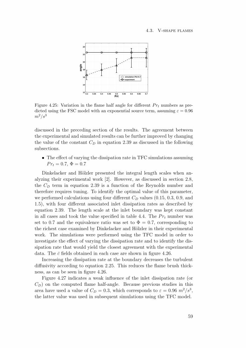
4.3. V-shape flames
0.3 0.35 0.4 0.45 0.5 0.55 0.6 0.65 0.712
14
16
18
20
22
24
angl
e
Prt
simulation Phi=0.7experiment
Figure 4.25: Variation in the flame half angle for different Prt numbers as pre-dicted using the FSC model with an exponential source term, assuming ε = 0.96m2/s3
discussed in the preceding section of the results. The agreement betweenthe experimental and simulated results can be further improved by changingthe value of the constant CD in equation 2.39 as discussed in the followingsubsections.
• The effect of varying the dissipation rate in TFC simulations assumingPrt = 0.7, Φ = 0.7
Dinkelacker and Holzler presented the integral length scales when an-alyzing their experimental work [2]. However, as discussed in section 2.8,the CD term in equation 2.39 is a function of the Reynolds number andtherefore requires tuning. To identify the optimal value of this parameter,we performed calculations using four different CD values (0.15, 0.3, 0.9, and1.5), with four different associated inlet dissipation rates as described byequation 2.39. The length scale at the inlet boundary was kept constantin all cases and took the value specified in table 4.4. The Prt number wasset to 0.7 and the equivalence ratio was set to Φ = 0.7, corresponding tothe richest case examined by Dinkelacker and Holzler in their experimentalwork. The simulations were performed using the TFC model in order toinvestigate the effect of varying the dissipation rate and to identify the dis-sipation rate that would yield the closest agreement with the experimentaldata. The c fields obtained in each case are shown in figure 4.26.
Increasing the dissipation rate at the boundary decreases the turbulentdiffusivity according to equation 2.25. This reduces the flame brush thick-ness, as can be seen in figure 4.26.
Figure 4.27 indicates a weak influence of the inlet dissipation rate (orCD) on the computed flame half-angle. Because previous studies in thisarea have used a value of CD = 0.3, which corresponds to ε = 0.96 m2/s3,the latter value was used in subsequent simulations using the TFC model.
59

Chapter 4. Model validation
(a) CD=0.15 (b) CD=0.3 (c) CD=0.9 (d) CD=1.5
Figure 4.26: c fields obtained using the TFC model at Φ=0.7 and A=0.50 fordifferent dissipation rates
0.2 0.4 0.6 0.8 1 1.2 1.4 1.615
20
25
30
35
angl
e
CD
simulationexperiment
Figure 4.27: Plots of the flame half-angle against CD based on TFC simulationswith Prt = 0.7, at Φ = 0.7
• The effect of varying the dissipation rate in FSC simulations using anexponential source term and assuming Prt = 0.5
FSC simulations with an exponential source term were performed usingfour different dissipation rates that were selected based on four differentvalues of the constant CD. The Prt value was set to 0.3 and the value ofthe c3 in the k−ε model was set to 0. The effects of varying the dissipationrate on the outcomes of these simulations are shown in figures 4.28 and 4.29.
Increasing the dissipation rate decreases both Dt,∞ and τL which in totalleads to a decrease in time dependent turbulent diffusion. Consequentlyturbulent flame brush thickness reduces as shown in figure 4.28.
Increases in the dissipation rate decrease Dt,∞ and therefore τL. Conse-quently, the time-dependent term in equation 2.29 will increase, causing an
60
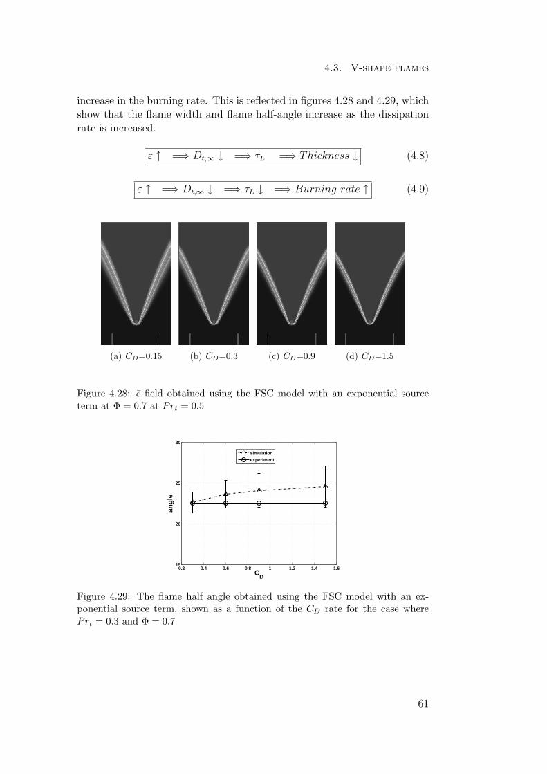
4.3. V-shape flames
increase in the burning rate. This is reflected in figures 4.28 and 4.29, whichshow that the flame width and flame half-angle increase as the dissipationrate is increased.
ε ↑ =⇒ Dt,∞ ↓ =⇒ τL =⇒ Thickness ↓ (4.8)
ε ↑ =⇒ Dt,∞ ↓ =⇒ τL ↓ =⇒ Burning rate ↑ (4.9)
(a) CD=0.15 (b) CD=0.3 (c) CD=0.9 (d) CD=1.5
Figure 4.28: c field obtained using the FSC model with an exponential sourceterm at Φ = 0.7 at Prt = 0.5
0.2 0.4 0.6 0.8 1 1.2 1.4 1.615
20
25
30
angl
e
CD
simulationexperiment
Figure 4.29: The flame half angle obtained using the FSC model with an ex-ponential source term, shown as a function of the CD rate for the case wherePrt = 0.3 and Φ = 0.7
61
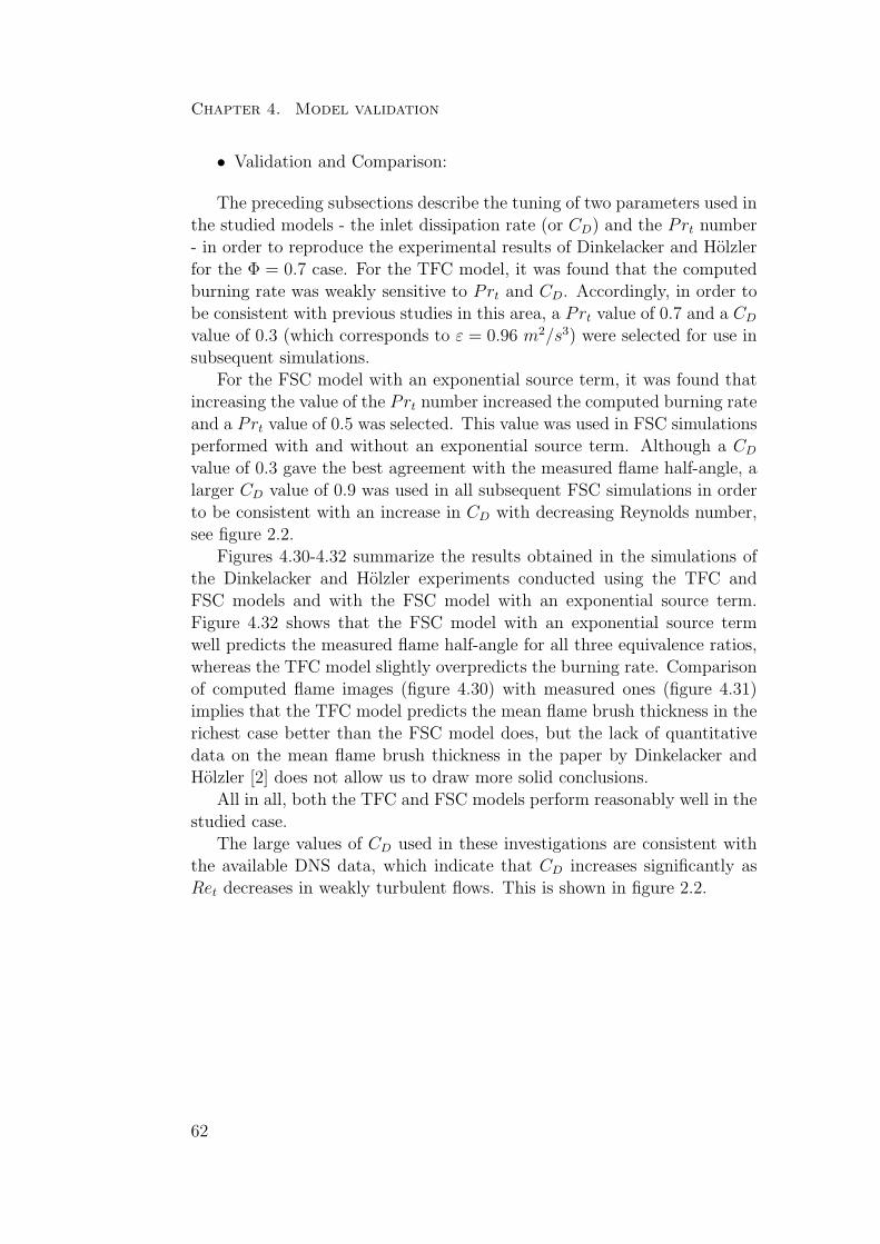
Chapter 4. Model validation
• Validation and Comparison:
The preceding subsections describe the tuning of two parameters used inthe studied models - the inlet dissipation rate (or CD) and the Prt number- in order to reproduce the experimental results of Dinkelacker and Holzlerfor the Φ = 0.7 case. For the TFC model, it was found that the computedburning rate was weakly sensitive to Prt and CD. Accordingly, in order tobe consistent with previous studies in this area, a Prt value of 0.7 and a CD
value of 0.3 (which corresponds to ε = 0.96 m2/s3) were selected for use insubsequent simulations.
For the FSC model with an exponential source term, it was found thatincreasing the value of the Prt number increased the computed burning rateand a Prt value of 0.5 was selected. This value was used in FSC simulationsperformed with and without an exponential source term. Although a CD
value of 0.3 gave the best agreement with the measured flame half-angle, alarger CD value of 0.9 was used in all subsequent FSC simulations in orderto be consistent with an increase in CD with decreasing Reynolds number,see figure 2.2.
Figures 4.30-4.32 summarize the results obtained in the simulations ofthe Dinkelacker and Holzler experiments conducted using the TFC andFSC models and with the FSC model with an exponential source term.Figure 4.32 shows that the FSC model with an exponential source termwell predicts the measured flame half-angle for all three equivalence ratios,whereas the TFC model slightly overpredicts the burning rate. Comparisonof computed flame images (figure 4.30) with measured ones (figure 4.31)implies that the TFC model predicts the mean flame brush thickness in therichest case better than the FSC model does, but the lack of quantitativedata on the mean flame brush thickness in the paper by Dinkelacker andHolzler [2] does not allow us to draw more solid conclusions.
All in all, both the TFC and FSC models perform reasonably well in thestudied case.
The large values of CD used in these investigations are consistent withthe available DNS data, which indicate that CD increases significantly asRet decreases in weakly turbulent flows. This is shown in figure 2.2.
62
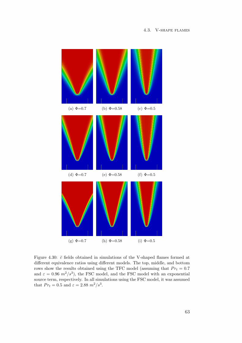
4.3. V-shape flames
(a) Φ=0.7 (b) Φ=0.58 (c) Φ=0.5
(d) Φ=0.7 (e) Φ=0.58 (f) Φ=0.5
(g) Φ=0.7 (h) Φ=0.58 (i) Φ=0.5
Figure 4.30: c fields obtained in simulations of the V-shaped flames formed atdifferent equivalence ratios using different models. The top, middle, and bottomrows show the results obtained using the TFC model (assuming that Prt = 0.7and ε = 0.96 m2/s3), the FSC model, and the FSC model with an exponentialsource term, respectively. In all simulations using the FSC model, it was assumedthat Prt = 0.5 and ε = 2.88 m2/s3.
63
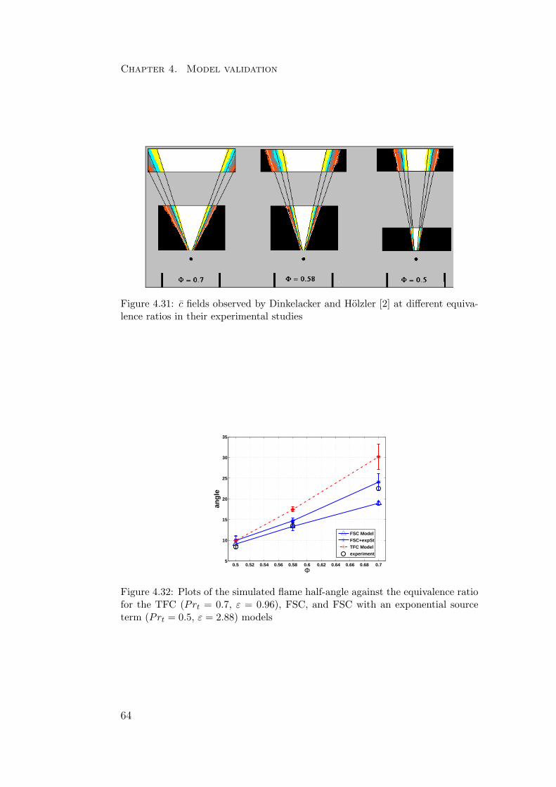
Chapter 4. Model validation
Figure 4.31: c fields observed by Dinkelacker and Holzler [2] at different equiva-lence ratios in their experimental studies
0.5 0.52 0.54 0.56 0.58 0.6 0.62 0.64 0.66 0.68 0.75
10
15
20
25
30
35
angl
e
Φ
FSC ModelFSC+expStTFC Modelexperiment
Figure 4.32: Plots of the simulated flame half-angle against the equivalence ratiofor the TFC (Prt = 0.7, ε = 0.96), FSC, and FSC with an exponential sourceterm (Prt = 0.5, ε = 2.88) models
64
Chapter 5
Concluding remarks and future
work
The OpenFOAM library was extended to simulate premixed turbulent com-bustion within the framework of the RANS paradigm. In particular, theoriginal library was found to yield an incorrect mean density for the reactingmixture and so a proper method for evaluating the mean density based onthe well-known equation 2.19 was implemented into the code. In addition,two well-known models (TFC and FSC) for describing the influence of tur-bulence on premixed combustion were also implemented into OpenFOAM.
The so-extended code was successfully applied to simulate two widelyrecognized sets of experiments with two substantially different, well-defined,simple, laboratory premixed turbulent flames, i.e. (i) the oblique, confined,preheated, highly turbulent methane-air flames experimentally studied byMoreau [1] and (ii) the V-shaped, open, weakly turbulent, lean methane-airflames investigated by Dinkelacker and Holzler [2] under the room condi-tions. In both sets of measurements, burning with different equivalenceratios was studied.
The computed results agree both qualitatively and quantitatively withthe aforementioned experimental data, thus, validating both the imple-mented combustion models and the extended code. A comparison of theresults computed using the TFC and FSC models, with all other thingsbeing equal, indicates that an early stage of premixed turbulent flame de-velopment, which is solely addressed by the latter model, plays a role byreducing the burning rate and mean flame brush thickness in the consideredcases.
It is worth stressing that the single constant A of the TFC and FSCmodels was not tuned in the present study, i.e. the same value of A = 0.5that is recommended in the literature was used in all of the simulations dis-cussed herein. However, in order to obtain the quantitative agreement with
65
Chapter 5. Concluding remarks and future work
the experimental results, two input parameters of the turbulence model, i.e.(i) the inlet dissipation rate and (ii) the turbulent Prandtl number, requiredtuning, because the available data on these two quantities are controversial.In the present work, these two input parameters were tuned for a singlereference case for each set of experiments and the same values were used tosimulate all other cases experimentally investigated either by Moreau [1] orby Dinkelacker and Holzler [2]. Therefore, these simulations showed thatboth models were capable of accurately and quantitatively predicting theeffects of variation in the equivalence ratio without requiring further tuning.
According to the schedule of the present project, the main focus of fu-ture work will be placed on (i) further extension of OpenFOAM library inorder to simulate turbulent scalar flux invoking recent advanced models forconditioned velocities in premixed turbulent flames and (ii) application ofthe so-extended code to multi-dimensional unsteady RANS simulations ofturbulent combustion in Direct Injection Stratified Charge Spark Ignitionengines. The demonstrated ability of the TFC and FSC models to wellpredict turbulent burning rates for various equivalence ratios makes thesetwo models particularly interesting for the latter purpose.
66
References
[1] P. Moreau, “Turbulent flame development in a high velocity pre-mixed flow,” in American Institute of Aeronautics and Astronautics,Aerospace Sciences Meeting, 15 th, Los Angeles, Calif, 1977.
[2] F. Dinkelacker and S. Holzler, “Investigation of a turbulent flame speedclosure approach for premixed flame calculations,” Combustion scienceand technology, vol. 158, no. 1, pp. 321–340, 2000.
[3] D. Spalding, “Mixing and chemical reaction in steady confined tur-bulent flames,” in Symposium (International) on Combustion, vol. 13,no. 1. Elsevier, 1971, pp. 649–657.
[4] B. F. Magnussen and B. H. Hjertager, “On mathematical modelingof turbulent combustion with special emphasis on soot formation andcombustion,” in Symposium (International) on Combustion, vol. 16,no. 1. Elsevier, 1977, pp. 719–729.
[5] V. Zimont and A. Lipatnikov, “A numerical model of premixed tur-bulent combustion of gases,” Chem. Phys. Reports, vol. 14, no. 7, pp.993–1025, 1995.
[6] A. Lipatnikov and J. Chomiak, “Turbulent flame speed and thickness:phenomenology, evaluation, and application in multi-dimensional sim-ulations,” Progress in energy and combustion science, vol. 28, no. 1,pp. 1–74, 2002.
[7] P. Sathiah and A. Lipatnikov, “Effects of turbulent flame speed de-velopment and axial convective waves on oscillations of a long ductedflame,” Combustion Science and Technology, vol. 179, no. 7, pp. 1433–1449, 2007.
[8] K. Bray and J. Moss, “A unified statistical model of the premixedturbulent flame,” Acta Astronautica, vol. 4, no. 3, pp. 291–319, 1977.
[9] P. A. Libby and K. Bray, “Variable density effects in premixed turbu-lent flames,” AIAA Journal, vol. 15, no. 8, pp. 1186–1193, 1977.
67
References
[10] A. Prudnikov, “Combustion of homogeneous fuel-air mixtures in tur-bulent flows,” Physical basis of processes in combustion chambers ofairbreathing engines. Moscow: Mashinostroenie, pp. 255–347, 1964.
[11] A. Prudnikov, “Hydrodynamics equations in turbulent flames,” Com-bustion in a turbulent flow. Moscow: Oborongiz, chapter 1, pp. 7–29,1960.
[12] V. Zimont, “Theory of turbulent combustion of a homogeneous fuelmixture at high reynolds numbers,” Combustion, explosion, and shockwaves, vol. 15, no. 3, pp. 305–311, 1979.
[13] V. L. Zimont, F. Biagioli, and K. Syed, “Modelling turbulent premixedcombustion in the intermediate steady propagation regime,” Progressin Computational Fluid Dynamics, An International Journal, vol. 1,no. 1, pp. 14–28, 2001.
[14] V. L. Zimont and F. Biagioli, “Gradient, counter-gradient transportand their transition in turbulent premixed flames,” Combustion Theoryand Modelling, vol. 6, no. 1, pp. 79–101, 2002.
[15] A. Lipatnikov, “Burning rate in impinging jet flames,” Journal of Com-bustion, vol. 2011, 2011.
[16] V. Sabelnikov and A. Lipatnikov, “Towards an extension of tfc modelof premixed turbulent combustion,” Flow, Turbulence and Combustion,pp. 1–14, 2012.
[17] A. Lipatnikov and J. Chomiak, “A simple model of unsteady turbulentflame propagation,” SAE transactions, vol. 106, no. 3, pp. 2441–2452,1997.
[18] A. Lipatnikov and J. Chomiak, “Transient and geometrical effects inexpanding turbulent flames,” Combustion science and technology, vol.154, no. 1, pp. 75–117, 2000.
[19] I. Zeldovich, G. I. Barenblatt, V. Librovich, and G. Makhviladze,“Mathematical theory of combustion and explosions,” 1985.
[20] E. Shchetinkov, “Physics of gas combustion,” 1965.
[21] R. S. Brodkey, “Fluid motion and mixing,” Mixing Theory and Prac-tice, vol. 1, pp. 7–110, 1966.
[22] S. B. Pope, Turbulent flows. Cambridge university press, 2000.
68
References
[23] R. N. Dahms, M. C. Drake, T. D. Fansler, T.-W. Kuo, and N. Pe-ters, “Understanding ignition processes in spray-guided gasoline en-gines using high-speed imaging and the extended spark-ignition modelsparkcimm. part a: Spark channel processes and the turbulent flamefront propagation,” Combustion and flame, vol. 158, no. 11, pp. 2229–2244, 2011.
[24] K. R. Sreenivasan, “An update on the energy dissipation rate inisotropic turbulence,” Physics of Fluids, vol. 10, p. 528, 1998.
[25] P. Yeung, D. Donzis, and K. Sreenivasan, “High-reynolds-number sim-ulation of turbulent mixing,” Physics of Fluids, vol. 17, p. 081703,2005.
[26] P. Yeung and S. Pope, “Lagrangian statistics from direct numericalsimulations of isotropic turbulence,” Journal of Fluid Mechanics, vol.207, no. 1, pp. 531–586, 1989.
[27] P. Yeung, “Lagrangian investigations of turbulence,” Annual review offluid mechanics, vol. 34, no. 1, pp. 115–142, 2002.
[28] D. Spalding, “Concentration fluctuations in a round turbulent free jet,”Chemical Engineering Science, vol. 26, no. 1, pp. 95–107, 1971.
[29] B. Launder, “Heat and mass transport,” in Turbulence. Springer,1978, pp. 231–287.
[30] A. Reynolds, “The prediction of turbulent prandtl and schmidt num-bers,” International Journal of Heat and Mass Transfer, vol. 18, no. 9,pp. 1055–1069, 1975.
[31] K. Koeltzsch, “The height dependence of the turbulent schmidt numberwithin the boundary layer,” Atmospheric Environment, vol. 34, no. 7,pp. 1147–1151, 2000.
[32] T. K. Flesch, J. H. Prueger, and J. L. Hatfield, “Turbulent schmidtnumber from a tracer experiment,” Agricultural and Forest Meteorol-ogy, vol. 111, no. 4, pp. 299–307, 2002.
[33] R. Bilger, L. Saetran, and L. Krishnamoorthy, “Reaction in a scalarmixing layer,” Journal of Fluid Mechanics, vol. 233, pp. 211–242, 1991.
[34] R. Borghi and P. Moreau, “Turbulent combustion in a premixed flow,”Acta Astronautica, vol. 4, no. 3, pp. 321–341, 1977.
69
References
[35] L. Maciocco and V. Zimont, “Test of the TFC Combustion Model onHigh Velocity Premixed CH4-Air Combustion in a Channel,” in Proc.20th Annual Meeting of the Italian Section of the Combustion Institute“Frantic97”, Cagliari, Italy, 1997, pp. X–2.1–2.4.
[36] V. Zimont and V. Battaglia, “Joint rans/les approach to premixedflame modelling in the context of the tfc combustion model,” Flow,turbulence and combustion, vol. 77, no. 1-4, pp. 305–331, 2006.
[37] F. Ghirelli, “Turbulent premixed flame model based on a recent dis-persion model,” Computers & Fluids, vol. 44, no. 1, pp. 369–376, 2011.
[38] F. Ghirelli, “Eulerian modeling of turbulent dispersion from a pointsource,” Computers & Fluids, vol. 38, no. 9, pp. 1795–1798, 2009.
[39] B. Launder and D. Spalding, “Mathematical Models of Turbulence,”Academic Press, 1972.
[40] R. J. Kee, J. F. Grcar, M. Smooke, and J. Miller, “Premix: a for-tran program for modeling steady laminar one-dimensional premixedflames,” Tech. Rep., 1985.
[41] G. Smith, M. Golden, M. Frenklach, N. Moriarty, B. Eiteneer, M. Gold-enberg, C. Bowman, R. Hanson, S. Song, W. Gardiner, V. Lissianski,and Z. Qin, “http://www.me.berkeley.edu/gri mech/.”
[42] R. J. Kee, J. A. Miller, and T. H. Jefferson, CHEMKIN: A general-purpose, problem-independent, transportable, FORTRAN chemical ki-netics code package. Sandia Laboratories, 1980.
[43] B. Launder and B. Sharma, “Application of the energy-dissipationmodel of turbulence to the calculation of flow near a spinning disc,”Letters Heat Mass Transfer, vol. 1, pp. 131–137, 1974.
[44] V. Yakhot, S. Orszag, S. Thangam, T. Gatski, and C. Speziale, “De-velopment of turbulence models for shear flows by a double expansiontechnique,” Physics of Fluids A: Fluid Dynamics, vol. 4, p. 1510, 1992.
[45] T.-H. Shih, W. Liou, A. Shabbir, Z. Yang, and J. Zhu, “A new k-epsiloneddy viscosity model for high reynolds number turbulent flows: Modeldevelopment and validation,” NASA STI/Recon Technical Report N,vol. 95, p. 11442, 1994.
[46] V. Moreau, “Progress in the self-similar turbulent flame premixed com-bustion model,” Applied Mathematical Modelling, vol. 34, no. 12, pp.4074–4088, 2010.
70

References
[47] V. Moreau, “A self-similar premixed turbulent flame model,” AppliedMathematical Modelling, vol. 33, no. 2, pp. 835–851, 2009.
71