003679-002

1

EXTENDED ESSAY IN MATHEMATICS SL

Spiral Forms in Nature

Can chosen spiral forms in nature be described using the logarithmic spiral?

Word count: 3 912

MAY 2013

003679-002

2

Abstract

The aim of this essay is to answer the following research question: “Can chosen spiral forms

in nature be described using the logarithmic spiral?”.

I have chosen to investigate this spiral in two dimensional space only, because focusing on

both two and three dimensional spaces in the essay would make me investigate the problem

partially and briefly.

In order to answer my research question I analysed in chapter 1 the properties of the

logarithmic spiral. In chapter 2 I chose photos of natural forms that made me think of the

logarithmic spiral: a shell, a chameleon’s tail, the Milky Way and the human ear. I measured

them accurately. The measurements were used to construct mathematical models of spirals. In

chapter 2 I also checked whether the models fit the original forms.

It turns out that most of the forms could be, more or less accurately, described using the

logarithmic spiral. This small discovery implicates that maybe other natural forms could be

described using other models or formulas. This leads to a hypothesis that nature could be

strongly connected to mathematics.

I believe that the subject is worth investigating because it emphasizes the true beauty of

mathematics and shows that maths can produce beautiful decorative forms.

003679-002

3

Table of contents

Introduction.................................................................................................................4

Chapter 1: The logarithmic spiral in two dimensional space and its properties..........6

1.1. A brief insight into history....................................................................................6

1.2. The definition of a spiral.......................................................................................7

1.3. The polar form of the logarithmic spiral...............................................................7

1.4. The cartesian form of the logarithmic spiral.........................................................8

1.5.Descartes’ theorem and its proof..........................................................................11

1.6.The impact of chosen parameters onto the shape of the spiral.............................12

Chapter 2: Mathematical analysis of natural spiral forms..........................................16

2.1. Nautilidae.............................................................................................................16

2.2. Chamaeleo calyptratus’ tail..................................................................................20

2.3. Milky way............................................................................................................23

2.4. Human ear............................................................................................................28

2.5. Further examples..................................................................................................30

Conclusion...................................................................................................................32

Bibliography................................................................................................................33

References...................................................................................................................34

003679-002

4

Introduction

In front of my high school (Juliusz Słowacki’s High School in Kielce, Poland) a specifical

sculpture can be found. This sculpture (Figure 1) was carved by a local artist, Józef

Sobczyński (1947 – 2008)1, and it represents two amonnites (extinct molluscs).

Figure 1. Jóżef Sobczyński’s amonnites

Every time I was passing nearby, I kept wondering whether their shape, repeated so many

times in nature, can be described in a mathematical way. My own interest in conchology led

me to the hypothesis that the shells are built on the basis of logarithmic spiral, which I

accidentally encountered in Fernando Corbalán’s book about the golden ratio2. I decided I

wanted to check on my own if its true and discover whether other spiral forms present in

nature can be described in a similar way. Hence my research question is: “Can chosen natural

forms be described using the logarithmic spiral?”. To answer it I will carefully analyse the

mathematical and geometrical properties of the logarithmic spiral in two-dimensional space

and compare it to the chosen photos or drawings of e.g. a shell, a chameleon’s tail. In my

opinion these objects will be similar to the logarithmic spiral.

003679-002

5

In this essay I hope to show the beauty of maths and prove that it isn’t limited to equations,

formulas and economics only, but can be found worldwide, in human ear and hurricanes; in

other words I want to show its universality. This is another reason why I find the phenomenon

of logarithmic spiral worth investigating.

003679-002

6

Chapter 1: The logarithmic spiral and its properties

1.1. A brief insight into history

The name “logarithmic spiral” arises from the transformation of the formula describing the

shape of the spiral. In this formula, if I express the angle in terms of the radius, I will obtain a

logarithm function.

Other names (e.g. “growth spiral”, “equiangular spiral”3) are connected to spiral’s properties.

The others need some historical background to be understood.

The logarithmic spiral appeared in human arts as early as in antiquity (ionic column capitals

in Greek architecture), but it has become popular as late as in 16th

century. The first

descriptions from the mathematical point of view were introduced by René Descartes (1596 -

1650). He noticed that while the spiral’s polar angles increase in arithmetical progression, its

radii increase in geometrical progression4 (“geometrical spiral”). Italian physician Evangelista

Torricelli (1608 – 1647) in his research managed to find the rectification of the curve5 and

English architect Sir Christopher Wren (1632 – 1723) suggested that the spiral could be “a

cone coiled about an axis”6.

English astronomer Edmond Halley (1656 – 1742) discovered that the spiral’s fragments cut

off in successive turns in proportion (“proportional” spiral) are self-similar7. Jacob Bernoulli

(1654 – 1705) was also fascinated by its self-similarity and thus named it “miraculous” spiral

(Spira mirabilis in Latin)8.

The logarithmic spiral is sometimes confused with the golden spiral, they are however not the

same.

003679-002

7

1.2. The definition of a spiral

In order to understand the definition of the logarithmic spiral better, I suggest taking a look at

the definition of a non-specified two-dimensional spiral:

A spiral “may be described most easily using polar coordinates, where the radius r is a

monotonic continuous function of angle θ” 9

.

1.3. The polar form of the logarithmic spiral

Figure 2.10

Logarithmic spiral

The logarithmic spiral is normally represented in the polar coordinate system. In such a

system the coordinates are the radius (r) and the chosen angle ( )11. The

generatrix (G) is a point that lays on the plane in distance r from the pole (described also as

origin, O). r depends on the angle (it has its vertex in the origin and the arm that starts its

turn is the ray OX (a polar axis))12

.

Therefore the logarithmic spiral is defined by the following formula13:

(1) ( )

003679-002

8

Where:

a, b – constant real parameters

At this point we can draw the logarithmic spiral with help of a graphic data calculator, Ti-84.

We change degrees to radians and Cartesian Plane to the polar coordinate system (POL). I

assumed that , and a=1, b=0.2. 1 Such a choice of values for these parameters

will be explained later in the essay. I inserted formula (1) in menu Y= and drew the spiral

(Figure 3.).

Figure 3. Construction of the logarithmic spiral in Ti-84

1.4. The cartesian form of the logarithmic spiral

Now I will derive the parametric equation of the logarithmic spiral in a cartesian coordinate

system.

Figure 4. Parameters x and y.

From Figure 4. it can be seen that:

and

003679-002

9

I multiply both equations by r.

and

Since ( ) (formula (1)),

Where (2) is the parametrical form of the logarithmic spiral.

Now I can draw the logarithmic spiral in Microsoft Excel. I will need this to check what

influence do different parameters have on the shape of the spiral and to be able to compare

them with examples from nature.

I will use a linear graph. Seven columns are needed (A – G)

In column A I put a set of angles: in our case, set A: A [-90 , 1080 ]. In column B I

transform degrees to radians (using this formula: “=PI()*A2/180”, where PI() is and A2 is

the cell number 2 in column A). Parameters a and b remain the same: a=1, b=0.2. Now, we

calculate the values in column E and F using formulas (1) and (2).

x=$C$92*EXP($D$92*B2)*COS(B2),

Where: $C$92 is the cell in which a=1 can be found, $D$92 is the cell with b = 0.2, B2 is the

angle in radians, and COS(B2) is the cosine of that angle. The Excel function EXP calculates

the value of e to the power of values in the brackets.

And y= $C$92*EXP($D$92*B2)*SIN(B2), where SIN(B2) is the sine of angle from the cell

B2.

The radius, r, is described by: r=$C$92*EXP($D$92*B2)

We should note that the cell B2 is not a constant and that it will change, from B2 till B1172

(they contain angles from set A).

Figure 5. shows a part of the data needed to construct the spiral.

003679-002

10

Figure 5. Part of the data needed to construct the spiral in Excel.

Now I draw the logarithmic spiral (Figure 6):

Figure 6. The logarithmic spiral in Excel

003679-002

11

1.5. Descartes’ theorem and its proof

Descartes’ Theorem:

“(in logarithmic spiral) the angle at which a radius increases in geometrical progression, as its

polar angle increases in arithmetical progression”14

Let U1 be an angle and first term in a sequence, and Un and Un+1 be the consecutive terms in

the same arithmetic sequence:

(3) Un = U1 + d(n-1)

(4) Un+1 = U1 + d(n)

and let d be common difference:

d = const

and let a and b be real numbers.

If Un and Un+1 are angles, we can apply them to the formula (1) creating the next terms of a

sequence of radii:

rn = ( ( ))

rn+1 = ( )

Let’s calculate the common ratio (q) for two consecutive terms of radii:

q = ( )

( ) =

( )

( ( )) =

( ) =

( ) =

= – ( ) = – =

Which means that q = const, so this is a geometric sequence.

003679-002

12

1.6. The impact of chosen parameters onto the shape of the spiral

Both parameters a and b are factors that change the value of the radius. Parameter a

multiplicates the whole expression, while parameter b multiplicates only the angle . This

may influence the shape of the curve. After a series of experiments I established that the most

suitable (the ones that ensure our curve will resemble a logarithmic spiral

like the one from Figure 2.) values of a and b are a=1 and b=0.2.

Now I will analyse the impact of parameters from different sets of numbers on the shape of

the spiral.

CASE 1

Parameters: a = 0, b = 0.2

( )

Since the radius equals zero, no curve can be drawn. The graph is empty.

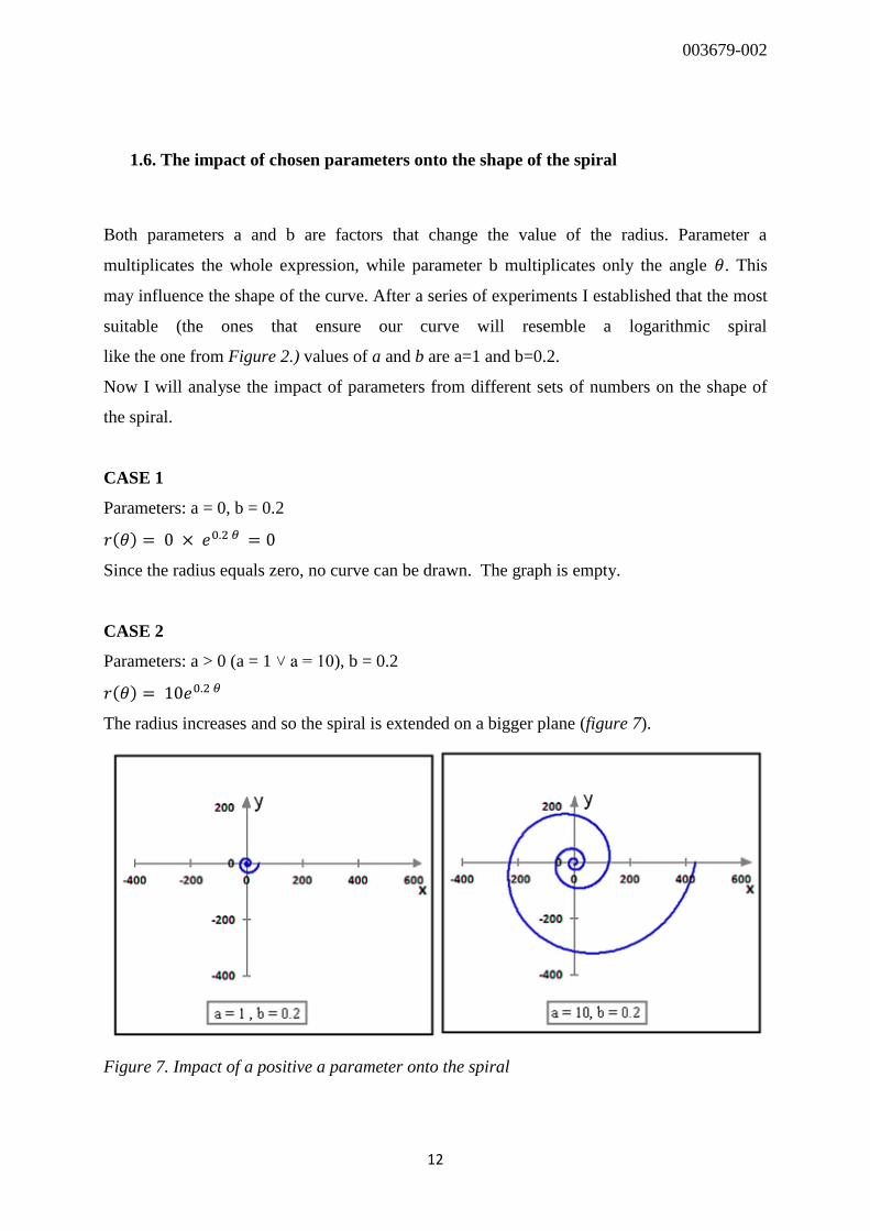
CASE 2

Parameters: a > 0 (a = 1 ˅ a = 10), b = 0.2

( )

The radius increases and so the spiral is extended on a bigger plane (figure 7).

Figure 7. Impact of a positive a parameter onto the spiral

003679-002

13

CASE 3

Parameters: a < 0 (e.g. a = - 10), b = 0.2

( )

The radius of the spiral increases and the spiral extents on a bigger plane, like in CASE 2.

However, since the values of a are negative, the spiral is centrally symmetrical to the spiral of

parameters a > 0 and b = 0.2 (Figure 8). The centre is the origin (0,0).

Figure 8. Impact of a negative a parameter onto the spiral

CASE 4

Parameters: a = 1, b > 0 (e.g. 0.4 ; 1)

( ) , ( )

The greater b, the greater the radius and as the angles increase, the spiral extents on a greater

and greater plane, swirling on an increasing distance from the origin (Figure 9.)

Figure 9. Impact of a positive b parameter onto the spiral

003679-002

14

CASE 5

Parameters: a=1, 0<b<1 (e.g. 0.1 ; 0.05 ; 0.01)

( ) , ( ) , ( )

The smaller b, the smaller the radius as the angles increase and so the spiral twirls to the

inside around the origin (Figure 10). When b is about to reach zero from both positive and

negative side, next turns of the spiral get closer to one another.

Figure 10. Impact of parameter b, when 0<b<1, onto the shape of the spiral

003679-002

15

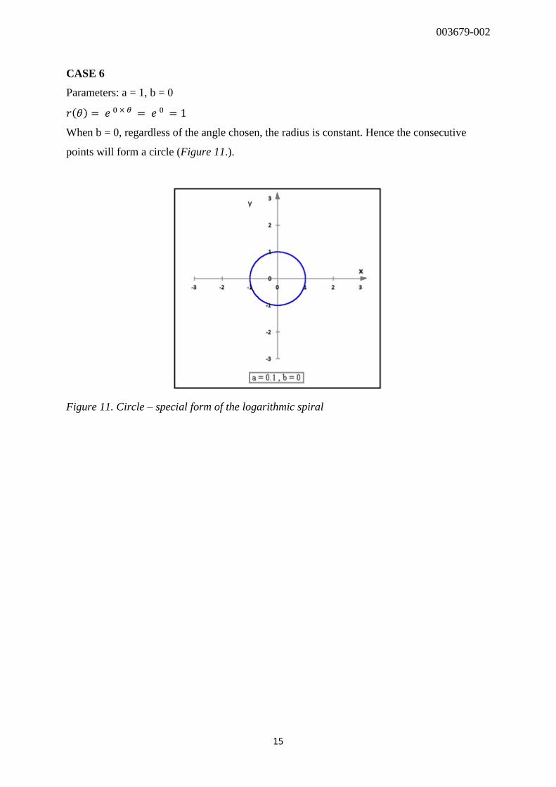
CASE 6

Parameters: a = 1, b = 0

( )

When b = 0, regardless of the angle chosen, the radius is constant. Hence the consecutive

points will form a circle (Figure 11.).

Figure 11. Circle – special form of the logarithmic spiral

003679-002

16

Chapter 2: Mathematical analysis of natural spiral forms

Now that I analysed the logarithmic spiral’s properties, I can proceed towards mathematical

analysis of chosen natural forms. In this chapter I hope to answer my research question.

2.1. Nautilidae

Nautilidae are marine molluscs. They live in warms seas near Indonesia. Figure 12. shows a

pendulum made of a Nautilius’ shell.

Figure 12. Pendulum made of a Nautilius’ shell

In order to see, whether this shell can be described using the logarithmic spiral, I will mark

the origin (white spot) and two chosen consecutive turns (yellow and blue spots) on the shell

(Figure 13):

003679-002

17

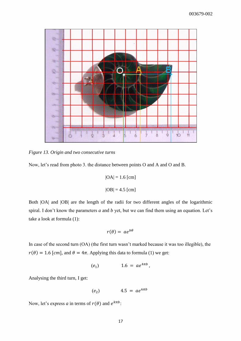
Figure 13. Origin and two consecutive turns

Now, let’s read from photo 3. the distance between points O and A and O and B.

|OA| = 1.6 [cm]

|OB| = 4.5 [cm]

Both |OA| and |OB| are the length of the radii for two different angles of the logarithmic

spiral. I don’t know the parameters a and b yet, but we can find them using an equation. Let’s

take a look at formula (1):

( )

In case of the second turn (OA) (the first turn wasn’t marked because it was too illegible), the

( ) , and . Applying this data to formula (1) we get:

( ) ,

Analysing the third turn, I get:

( )

Now, let’s express a in terms of ( ) and :

003679-002

18

from ( )

from ( )

I get the following equation:

( )

( )

Since ,

We divided the upper equation by and get b:

Now that we have b, we should also find a. Let’s use the equation derivated before from ( ):

( )

At this point we have all the data needed to find the logarithmic spiral that should fit the

nautilus’ shell. Figure 14. on the next page shows it:

003679-002

19

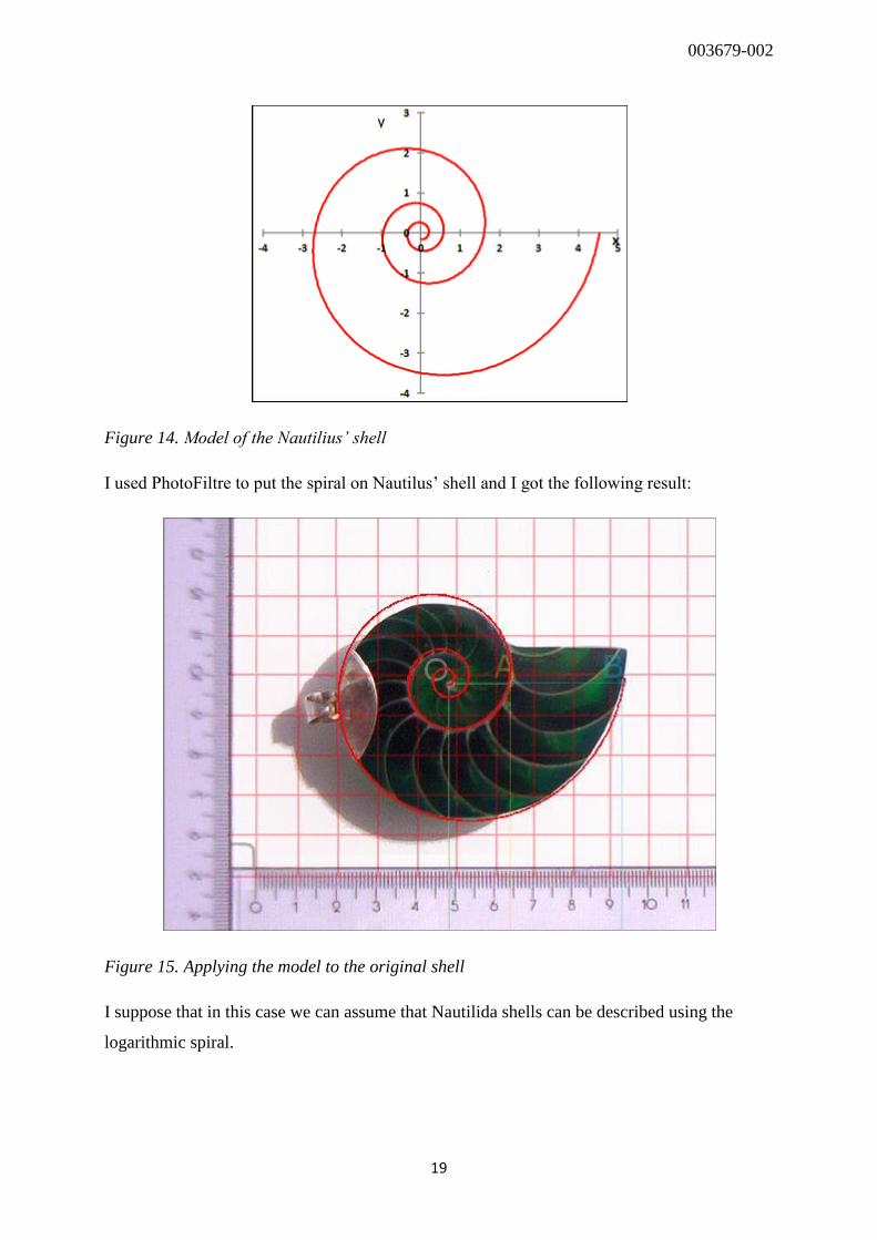
Figure 14. Model of the Nautilius’ shell

I used PhotoFiltre to put the spiral on Nautilus’ shell and I got the following result:

Figure 15. Applying the model to the original shell

I suppose that in this case we can assume that Nautilida shells can be described using the

logarithmic spiral.

003679-002

20

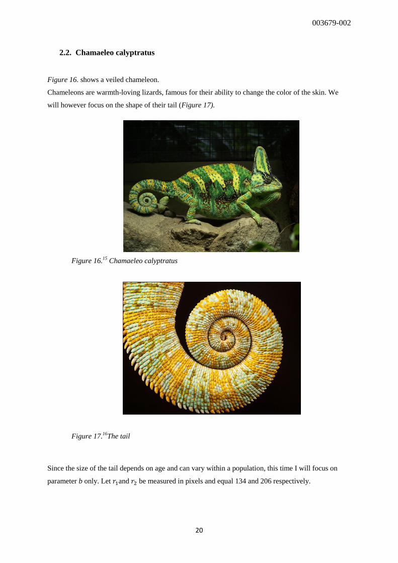
2.2. Chamaeleo calyptratus

Figure 16. shows a veiled chameleon.

Chameleons are warmth-loving lizards, famous for their ability to change the color of the skin. We

will however focus on the shape of their tail (Figure 17).

Figure 16.15

Chamaeleo calyptratus

Figure 17.16

The tail

Since the size of the tail depends on age and can vary within a population, this time I will focus on

parameter b only. Let and be measured in pixels and equal 134 and 206 respectively.

003679-002

21

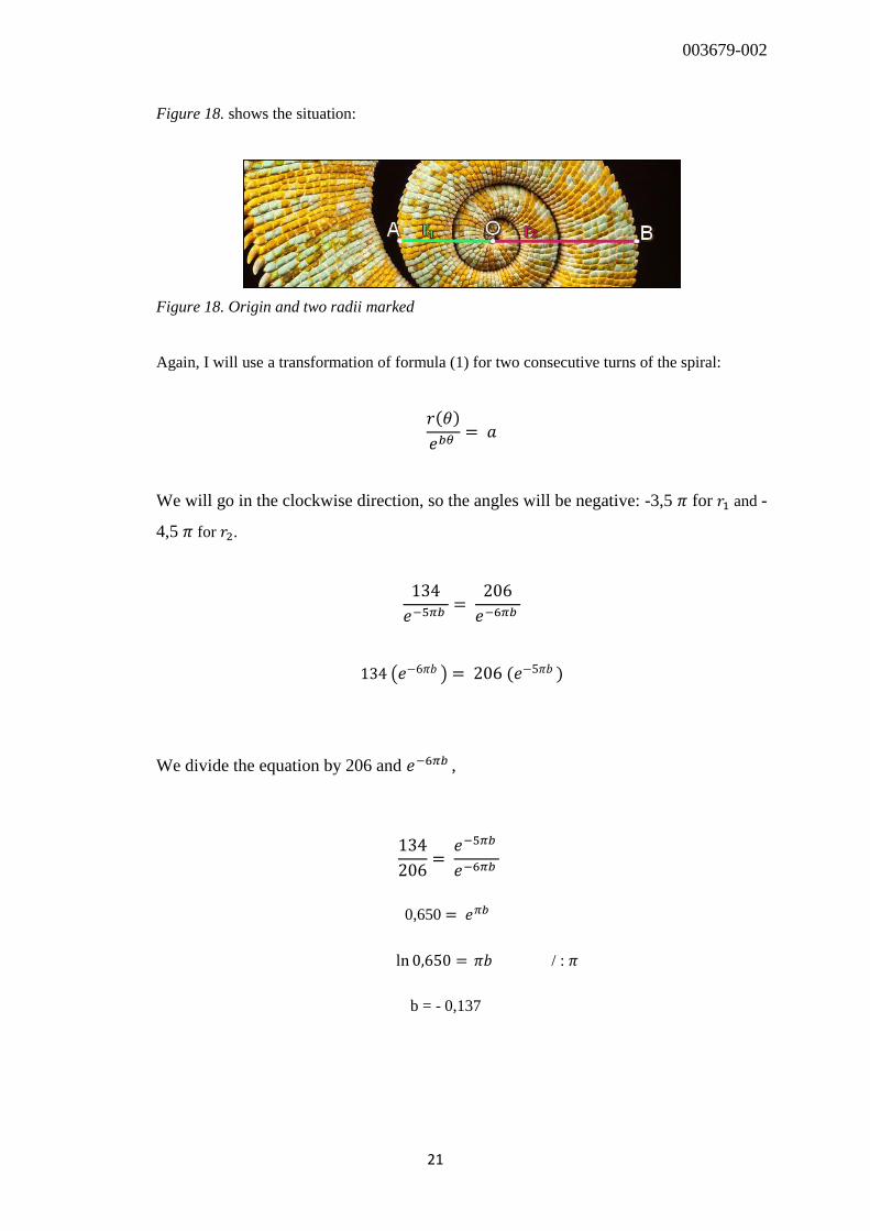
Figure 18. shows the situation:

Figure 18. Origin and two radii marked

Again, I will use a transformation of formula (1) for two consecutive turns of the spiral:

( )

We will go in the clockwise direction, so the angles will be negative: -3,5 for and -

4,5 for .

( ) ( )

We divide the equation by 206 and ,

0,650

/ :

b = - 0,137

003679-002

22

Choosing a random, greater than zero a (in my case a = 11) and applying it together with

parameter b to my excel equations I get such a graph:

Figure 19. Model of the tail

I placed the graph on the photo and got the following result:

Figure 20. Applying the model to the tail

I suppose that this time a natural form can be described using the logarithmic spiral, too.

003679-002

23

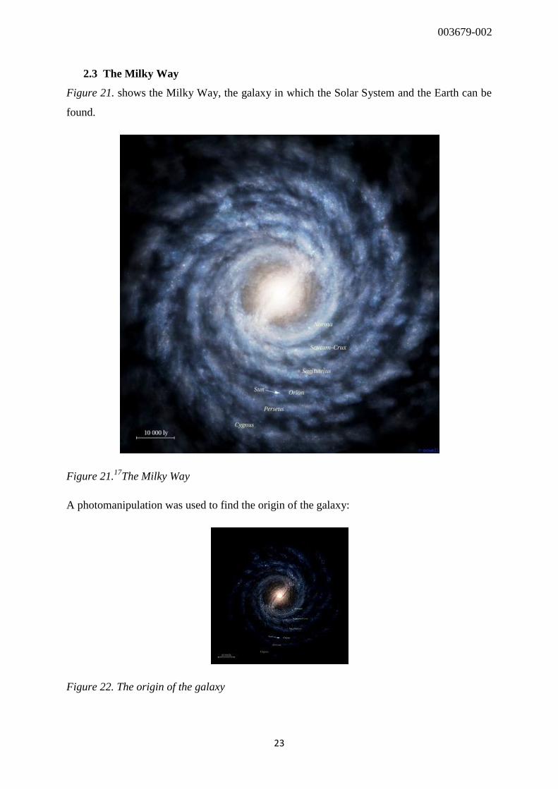
2.3 The Milky Way

Figure 21. shows the Milky Way, the galaxy in which the Solar System and the Earth can be

found.

Figure 21.17

The Milky Way

A photomanipulation was used to find the origin of the galaxy:

Figure 22. The origin of the galaxy

003679-002

24

Each 95 pixels on the picture 6. correspond to 10 000 light years. 1 light year (ly) is

approximately 9,4607·1015 m. I decided to use the ly unit, because Excel's possibilites are

limited when it comes to counting bigger numbers.

To find whether the galaxy can be described using a logarithmic spiral I traced a sample curve

and marked the O point in the centre of the region marked as origin (O). Then like in previous

cases I drew two line segments – ⃗⃗⃗⃗ ⃗ ( ) and ⃗⃗ ⃗⃗ ⃗ ( ). The angle at which point A can be

found is

, and the angle for point B is at

. Figure 23. below shows the whole situation.

Figure 23. Origin and two radii

Counting the :

if: 95 px – 10 000 ly

then: 186 px (length of on the picture) –

[ly]

and its value is of .

003679-002

25

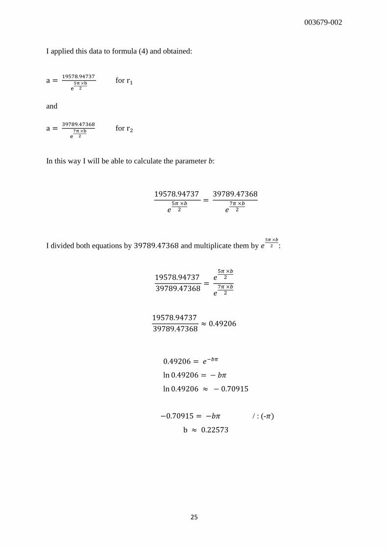
I applied this data to formula (4) and obtained:

for

and

for

In this way I will be able to calculate the parameter b:

I divided both equations by and multiplicate them by

:

/ : (- )

003679-002

26

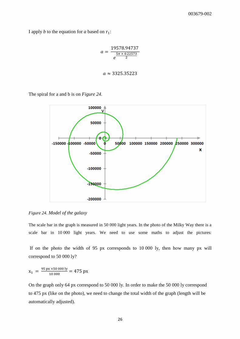
I apply b to the equation for a based on :

The spiral for a and b is on Figure 24.

Figure 24. Model of the galaxy

The scale bar in the graph is measured in 50 000 light years. In the photo of the Milky Way there is a

scale bar in 10 000 light years. We need to use some maths to adjust the pictures:

If on the photo the width of 95 px corresponds to 10 000 ly, then how many px will

correspond to 50 000 ly?

On the graph only 64 px correspond to 50 000 ly. In order to make the 50 000 ly correspond

to 475 px (like on the photo), we need to change the total width of the graph (length will be

automatically adjusted).

003679-002

27

if 64 px correspond to 475 px,

then 656 px (the total width of the graph) –

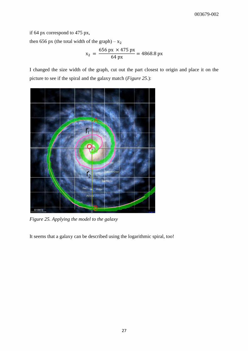
I changed the size width of the graph, cut out the part closest to origin and place it on the

picture to see if the spiral and the galaxy match (Figure 25.):

Figure 25. Applying the model to the galaxy

It seems that a galaxy can be described using the logarithmic spiral, too!

003679-002

28

2.4. The human ear

Can a part of human body be described using the spiral? Why not! Let’s try with the human

ear.

It however causes more problems than the previous examples because in this case there is no

real origin (figure 26.).

Figure 26. My ear

I decided to find the parameters by trial and error and I chose a = 0.700, b = 0.250. I took

angles from a new set: [-90 ; 273] degrees and let Excel draw the graph (Figure 27. on the

next page).

003679-002

29

Figure 27. Model of the human ear

The origin of the ear is the intersection point of lines and , passing through points

and , and and- respectively (figure 28.). However, I can’t prove that they

intersect and that the angle at which they intersect is a straight angle.

Figure 28. Searching for origin

We can still apply Figure 29 to the photo of human ear. The result obtained is not as

precised as in previous cases, but it matches the photo (Figure 29. on the next page):

003679-002

30

Figure 29. Applying the model to the ear

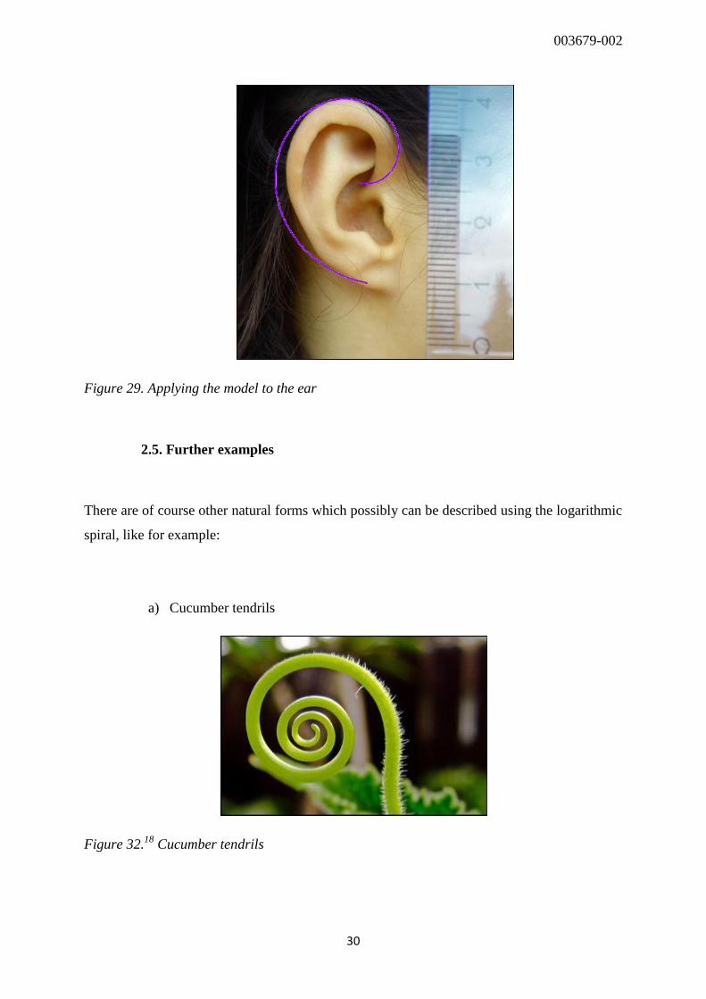
2.5. Further examples

There are of course other natural forms which possibly can be described using the logarithmic

spiral, like for example:

a) Cucumber tendrils

Figure 32.18

Cucumber tendrils

003679-002

31

b) Rex begonia leaves:

Figure 33.19

Rex begonia leaves

c) Half Moon Bay, California, USA20

:

Figure 34.21

Half Moon Bay

d) Pressure system over Iceland:

Figure 35.22

Pressure system over Iceland

003679-002

32

Conclusion

The aim of my essay was to check whether chosen natural forms could be described using the

logarithmic spiral. I managed to construct two-dimensional models which more or less

resembled the examples I chose to analyse. Therefore, the answer to my research question is

yes, natural forms can be described using the logarithmic spiral.

I am satisfied with my discovery. It changed my view on how the world is constructed. I

always thought nature was undescribable. What if it’s all about maths instead? We already

know that bacteria reproduce according to a logarithmic pattern. Snowflakes are similar to

fractals. What if we didn’t invent, but only discovered formulas?

I was convinced that I would most appreciate the decorative forms formulas can produce.

Now I see that there is something that enchants me more. This is the connection between

different areas of mathematics. Although this extended essay focused on logarithmic spiral, I

used some geometry, trigonometric functions, sequences and series and Excel maths.

Maths is truly universal.

003679-002

33

Bibliography

1. N., Siemienadiajew K.A., Musiol G., Mühlig H. Nowoczesne KOMPEDIUM

MATEMATYKI, Trans. Szczech A., Gorzecki M. Warsaw, Poland: Wydawnictwo

Naukowe PWN, 2004.

2. Pickover, C. A., (2009), The Math Book: From Pythagoras to the 57th Dimension,

250 Milestones in the History of Mathematics, Toronto, Canada: Sterling

Publishing

3. Corbalán, F. (2010)., Złota proporcja: Matematyczny język piękna [Golden ratio:

Mathematical language of beauty]. Warsaw, Poland: BUKA Books.

4. White, J., (2004), Calculus In Action: Microworld 8: Logarithmic Spirals and

Planetary Orbits. Bluejay Lispware, 2004. Mathematical Association of America.

Web. 9th

Jul. 2012.

5. Yronwode Caroline. “Sacred Geometry”. The sacred landscape. Luckymojo.com,

access on 9th

July 2012. Web.

6. Erbas Ayhan Kursat. “Spira Mirabilis”. Spira Mirabilis, Logarithmic Spiral,

Golden Spiral. Department of Math Education, University of Georgia, Athens,

GA, access on 9th

July 2012. Web.

7. Author unknown. “Logarithmic spiral”. Logarithmic spiral – the definition of

logarithmic spiral. Onlinedictionary.datasegment.com, access on 9th

July 2012.

Web.

8. Köller Jürgen. „Spirals”. Spirals. Mathematische-Basteleien.de, access on 9th

July

2012. Web.

9. Maślanka Krzysztof. “Ukryte ślady racjonalności przyrody”. Working papers.

Kul.pl, access on 9th

July 2012. Web.

10. Lucca Giovanni. “Un modello per le conchiglie”. 4. Un modello per le conchiglie |

conchiglie. Matematichamente.it, access on 9th

July 2012. Web.

11. Pischedda Carlo. „La spirale logarithmica”. Math.it – La spirale logarithmica.

Math.it, access on 9th

July 2012. Web.

12. Mathworld Team. “Logarithmic spiral”. Logarithmic spiral. Wolfram Alpha,

access on 9th

July 2012. Web.

13. Wikipedia, The Free Encyclopedia. Wikimedia Foundation, access on 9th

July

2012. Web.

003679-002

34

References:

1 “Józef Sobczyński.” Wikipedia: The Free Encyclopedia. Wikimedia Foundation, access on 23rd June 2012.

Web.

2 Corbalán, F. (2010)., Złota proporcja: Matematyczny język piękna [Golden ratio: Mathematical language of

beauty]. Warsaw, Poland: BUKA Books.

3 “Logarithmic spiral” Wikpedia: The Free Encyclopedia. Wikimedia Foundation, access on 23

rd June 2012.

Web.

4 Erbas Ayhan Kursat. “Spira Mirabilis”. Spira Mirabilis, Logarithmic Spiral, Golden Spiral. Department of

Math Education, University of Georgia, Athens, GA, access on 23rd June 2012. Web.

5 Pickover, C. A., (2009), The Math Book: From Pythagoras to the 57th Dimension, 250 Milestones in the

History of Mathematics, Toronto, Canada: Sterling Publishing

6 Erbas Ayhan Kursat. “Spira Mirabilis”. Spira Mirabilis, Logarithmic Spiral, Golden Spiral. Department of

Math Education, University of Georgia, Athens, GA, access on 24th June 2012. Web.

7 Erbas Ayhan Kursat. “Spira Mirabilis”. Spira Mirabilis, Logarithmic Spiral, Golden Spiral. Department of

Math Education, University of Georgia, Athens, GA, access on 24th June 2012. Web.

8 Erbas Ayhan Kursat. “Spira Mirabilis”. Spira Mirabilis, Logarithmic Spiral, Golden Spiral. Department of

Math Education, University of Georgia, Athens, GA, access on 24th June 2012. Web.

9 Answers Corporation. “spiral”. Spiral: definition, synonyms from Answers.com, Answers.com, access on 30

th

June 2012. Web.

10Weisstein, E. W. “Logarithmic Spiral”. From MathWorld - A Wolfram Web Resource, Wolfram Alpha, access

on 9th

July 2012. Web.

11 “Polar coordinate system.” Wikipedia: The Free Encyclopedia. Wikimedia Foundation, access on access on 9

th

July 2012. Web.

12 Author unknown. “Logarithmic spiral”. Logarithmic spiral – the definition of logarithmic spiral.

Onlinedictionary.datasegment.com, access on 9th

July 2012. Web.

13 Bronsztejn I. N., Siemienadiajew K.A., Musiol G., Mühlig H. Nowoczesne KOMPEDIUM MATEMATYKI,

Trans. Szczech A., Gorzecki M. Warsaw, Poland: Wydawnictwo Naukowe PWN, 2004.

14 Erbas Ayhan Kursat. “Spira Mirabilis”. Spira Mirabilis, Logarithmic Spiral, Golden Spiral. Department of

Math Education, University of Georgia, Athens, GA, access on 15th July 2012. Web.

15 World Association of Zoos and Aquariums WAZA, “Yemen Chamaeleon”, Yemen Chamaeleon: Chamaeleo

calypratus. Waza.org, access on 27th

August 2012. Web.

16 Abrook Rafe. Yemen Chameleon Tail. 2010. Access on 27

th August 2012. Web.

<http://www.flickriver.com/photos/rafeabrook/5231184593/>

17 Author Unknown. Milky Way. Date unknown. Access on 29

th August 2012. Web.

<http://wszechswiat.astrowww.pl/milkyway.jpg>

18 Tonyz20. Cucumber plants’ coiling ability. Date unknown. Access on 3

rd September 2012. Web.

<http://www.redorbit.com/news/science/1112685493/cucumber-spring-083112/>

003679-002

35

19

Author Unknown. Rex begonia. Date unknown. Access on 3rd

September 2012. Web. Access on 3rd

September

2012. Web. <http://www.logantrd.com/wp-content/uploads/2012/04/rex-begonia.jpg>

20 „Logarithmic spiral beaches” Wikipedia: The Free Encyclopedia. Wikimedia Foundation, access on 3

rd

September 2012. Web.

21 Author unknown. Half moon bay California. Date unknown. Access on 3

rd September 2012. Web.

<http://www.tripadvisor.com/LocationPhotos-g32469-Half_Moon_Bay_California.html#17942813v>

22 Wikipedia commons. Low pressure system over Iceland. Date unknown. Access on 3

rd September 2012. Web.

<http://upload.wikimedia.org/wikipedia/commons/thumb/b/bc/Low_pressure_system_over_Iceland.jpg/692px-

Low_pressure_system_over_Iceland.jpg>