Embed Size (px)
Citation preview
Express Misprediction Recovery
By
Vignyan Reddy Kothinti Naresh
A dissertation submitted in partial fulfillment of
the requirements for the degree of
Doctor of Philosophy
(Electrical and Computer Engineering)
at the
UNIVERSITY OF WISCONSIN–MADISON
2014
Date of final oral examination: 07/11/14
The dissertation is approved by the following members of the Final Oral Committee:
Mikko H. Lipasti, Professor, Electrical and Computer EngineeringKewal K. Saluja, Professor, Electrical and Computer EngineeringGurindar S. Sohi, Professor, Computer SciencesNam Sung Kim, Associate Professor, Electrical and Computer EngineeringKatherine L. Morrow, Associate Professor, Electrical and Computer Engi-neering

All rights reserved
INFORMATION TO ALL USERSThe quality of this reproduction is dependent upon the quality of the copy submitted.
In the unlikely event that the author did not send a complete manuscriptand there are missing pages, these will be noted. Also, if material had to be removed,
a note will indicate the deletion.
Microform Edition © ProQuest LLC.All rights reserved. This work is protected against
unauthorized copying under Title 17, United States Code
ProQuest LLC.789 East Eisenhower Parkway
P.O. Box 1346Ann Arbor, MI 48106 - 1346
UMI 3635514Published by ProQuest LLC (2014). Copyright in the Dissertation held by the Author.
UMI Number: 3635514

© Copyright by Vignyan Reddy Kothinti Naresh 2014
All Rights Reserved

i
This thesis is dedicated to my family for their endless love and support.

ii
acknowledgmentsI would like to acknowledge my family, professors and friends for their
support and guidance that led to manifestation of this thesis.
I would like to thank my family for their immense love and support
by dedicating this work. My parents, Uma Maheswari and Satyanarayana
Reddy, who have incessantly prioritized me over themselves are my divine
incarnation. A limitless debt of gratitude for my brother, Karthikeya Reddy,
who took over my share of family responsibilities to facilitate my aspirations.
Words fail in expressing my appreciation for my loving wife, Samatha, for
her concern, care, motivation and support.
I am deeply indebted to my advisor, Prof. Mikko H. Lipasti, for his
constant guidance, care and help throughout my doctoral pursuit. His
passion for exploring novel and practical solutions for challenging problems
has been inductive and I feel fortunate to be his student.
I want to thank Professors Kewal K. Saluja, Nam Sung Kim and Michael
J. Schulte for collaborating with me on various projects through my grad-
uate school. Their validation and support of my ideas in teaching and
research boosted my skillset and confidence. I also want to acknowledge
my professors and colleagues associated with computer architecture at the
University of Wisconsin-Madison for sharing their knowledge and experience.
Their commitment to several events and productive discusions helped in
understanding some obscure concepts and kindled new ideas.

iii
I would also like to thank my friends and colleagues who have provided
me with insightful discussions and fellowship. Special acknowledgements to
Mitchell Hayenga, David Palframan, Arslan Zulfiqar, Dibakar Gope, Syed
Gilani, Sean Franey, Andrew Nere, Zhong Zheng, Atif Hashmi and Erika
Gunadi for their friendship, collaboration, discussions and support.

iv
contents
Contents iv
List of Tables vii
List of Figures viii
Abstract xii
1 Introduction 1
1.1 Performance and Power Opportunity 4
1.2 Processor Pipelines and CRIB Refresher 8
1.3 EMR Overview 11
1.4 Thesis Contributions 13
1.5 Thesis Organization 15
2 Prior Art 16
2.1 Background 16
2.2 Reducing Misprediction Penalty 21
2.3 Execution Localized Scheduling Engines 29
2.4 CRIB 35
2.5 Summary 40
3 Express Misprediction Recovery 41
3.1 Motivating Example 41

v
3.2 Architectural Overview 43
3.3 Partition Control Unit 45
3.4 Demand Fetch 49
3.5 Back-End Branch Prediction 54
3.6 In-place Fetch and Misprediction Recovery 55
3.7 Summary 57
4 Control Independence 58
4.1 Discovering Control Independence 58
4.2 Trade Offs in Control Independence 62
4.3 Case Study of Astar 63
4.4 Summary 65
5 Amplified Instruction Delivery 66
5.1 Relaxing the Flynn’s Bottleneck Limit 66
5.2 Case Study of Libquantum 71
5.3 Summary 73
6 Evaluation 74
6.1 Evaluation Setup 74
6.2 Performance 81
6.3 Performance Sensitivity Analysis 91
6.4 Instruction Sources 98
6.5 Energy Analysis101

vi
6.6 Summary106
7 Conclusion108
7.1 Future Work110
Bibliography114

vii
list of tables
5.1 Example contents of Next-index predictor which is used to amplify
instruction delivery. . . . . . . . . . . . . . . . . . . . . . . . . . 70
6.1 Configurations of baseline machines and EMR. . . . . . . . . . . 76
6.2 Characteristics of simpoint regions of SPEC2006 benchmarks. . 79
6.3 Characteristics of MiBench and Graph500. . . . . . . . . . . . . 80

viii
list of figures
1.1 Power components of ARM A15 processor. . . . . . . . . . . . . 3
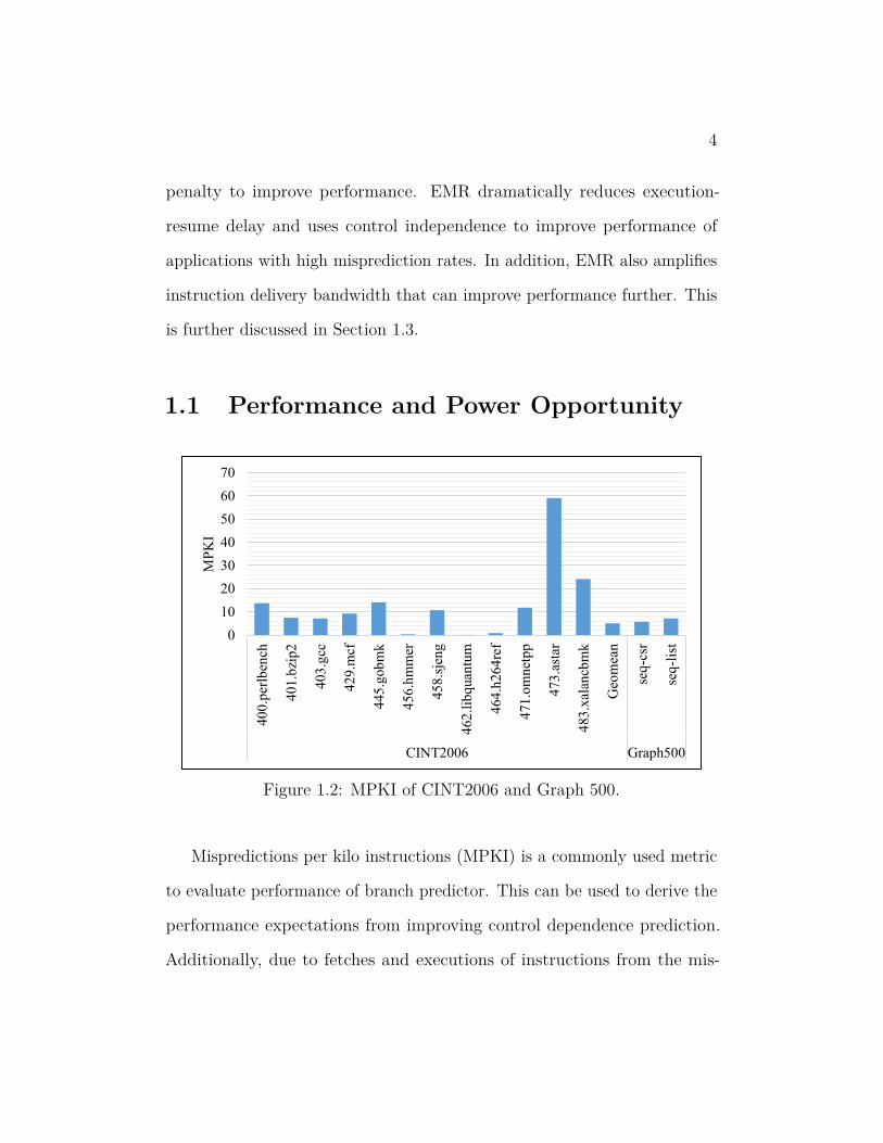
1.2 MPKI of CINT2006 and Graph 500. . . . . . . . . . . . . . . . 4
1.3 MPKI of CFP2006. . . . . . . . . . . . . . . . . . . . . . . . . . 5
1.4 MPKI of MiBench. . . . . . . . . . . . . . . . . . . . . . . . . . 6
1.5 Performance effects of Ideal branch prediction and doubling the
front end bandwidth (_X2). . . . . . . . . . . . . . . . . . . . . 7
1.6 Pipeline diagrams of the baseline conventional OoO, CRIB and
the proposed EMR processors. . . . . . . . . . . . . . . . . . . . 8
1.7 Block diagram of CRIB. . . . . . . . . . . . . . . . . . . . . . . 10
2.1 Some examples of control independence. . . . . . . . . . . . . . 23
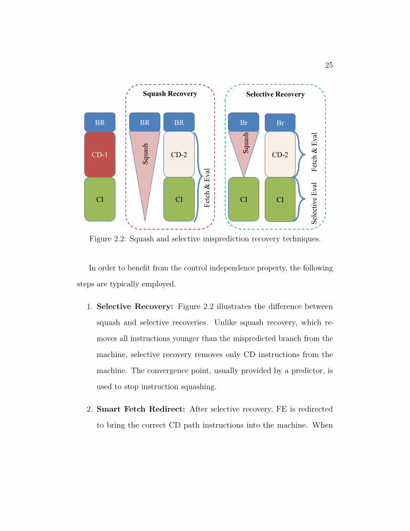
2.2 Squash and selective misprediction recovery techniques. . . . . . 25
2.3 Top level view of CRIB unit. . . . . . . . . . . . . . . . . . . . . 35
2.4 Internals of a CRIB partition. . . . . . . . . . . . . . . . . . . . 36
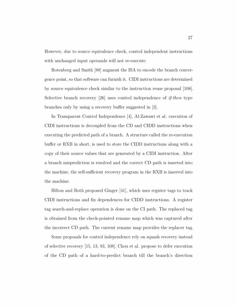
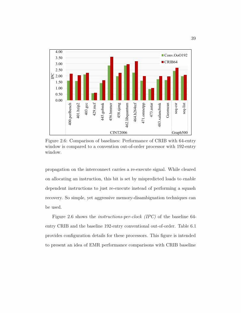
2.5 Internals of a CRIB execution station. . . . . . . . . . . . . . . 37
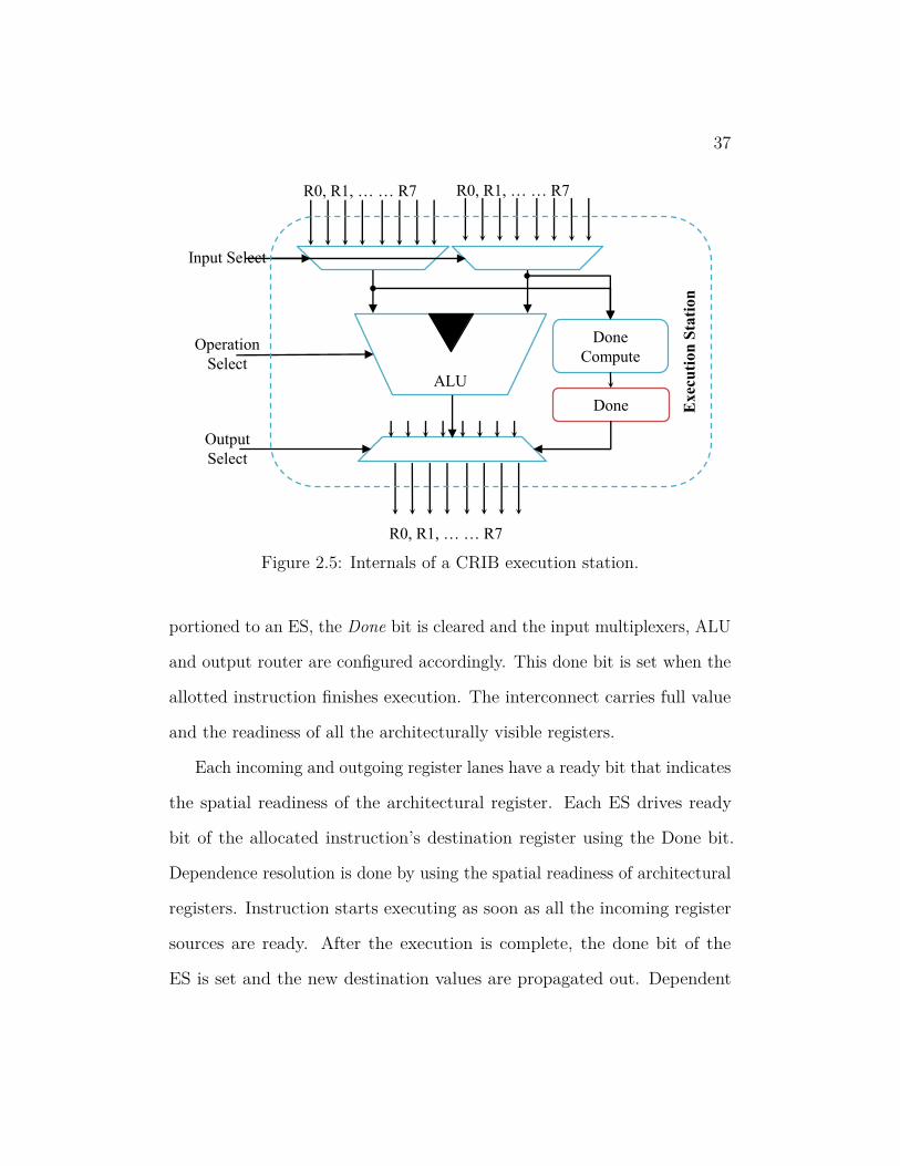
2.6 Comparison of baselines: Performance of CRIB with 64-entry
window is compared to a convention out-of-order processor with
192-entry window. . . . . . . . . . . . . . . . . . . . . . . . . . 39
3.1 Example illustrating basic EMR functionality. The branch with
L1 as the target is the mispredicted branch. . . . . . . . . . . . 42
3.2 Overview of EMR architecture. . . . . . . . . . . . . . . . . . . 44

ix
3.3 Control communication between the partition control unit. . . . 44
3.4 Internals of a partition control units. . . . . . . . . . . . . . . . 45
3.5 Components of demand fetch unit. . . . . . . . . . . . . . . . . 49
3.6 Finite state machine at the demand fetch unit that indicates the
state of the front-end. . . . . . . . . . . . . . . . . . . . . . . . 51
4.1 Example code with instruction address labels. . . . . . . . . . . 59
4.2 Examples of contents of select address table when two different
paths of a branch are selected. . . . . . . . . . . . . . . . . . . . 60
5.1 An example 462.libquantum’s loop as captured in a four partition
EMR. The NIP entries are also shown. . . . . . . . . . . . . . . 72
6.1 Performance advantage of EMR when compared to baseline CRIB
when executing CINT2006 and Graph500 benchmarks. . . . . . 82
6.2 Performance gains of EMR relative to the performance of baseline
CRIB when executing CFP2006. . . . . . . . . . . . . . . . . . 84
6.3 Relative performance of EMR when compared with baseline
CRIB while evaluating MiBench. . . . . . . . . . . . . . . . . . 85
6.4 Opportunity to amplify instruction delivery and the cumulative
accuracy of the next-index predictors in CINT2006 and Graph500
benchmarks. . . . . . . . . . . . . . . . . . . . . . . . . . . . . 87
6.5 AID opportunity and aggregated accuracy of the next-index
predictors when executing CFP2006 benchmarks. . . . . . . . . 88

x
6.6 Opportunity to amplify instruction delivery and the cumulative
accuracy of the next-index predictors for MiBench. . . . . . . . 89
6.7 Performance CRIB and EMR when scaling the window size. . . 90
6.8 No-ops per partition in different configurations of EMR for
MiBench. . . . . . . . . . . . . . . . . . . . . . . . . . . . . . . 91
6.9 Performance CRIB and EMR when scaling the window size. . . 92
6.10 Performance gains of EMR relative to baseline CRIB when vary-
ing LOC$ sizes. IB stands for Instruction Bundle. . . . . . . . . 93
6.11 Performance of EMR using different sizes of ICU$ when compared
to baseline CRIB using a 4096 entry µop cache. . . . . . . . . . 95
6.12 Split of instruction sources in EMR. . . . . . . . . . . . . . . . . 96
6.13 Performance gains of EMR over baseline CRIB when running
CINT2006 with varying ICU$ access time. . . . . . . . . . . . . 97
6.14 Split of instruction sources in EMR for CINT2006 and Graph500. 98
6.15 Split of instruction sources in EMR for CFP2006. . . . . . . . . 100
6.16 Split of instruction sources in EMR for MiBench. . . . . . . . . 101
6.17 Energy of EMR relative to CRIB baseline for CINT2006 and
Graph500. . . . . . . . . . . . . . . . . . . . . . . . . . . . . . . 102
6.18 Energy consumed by EMR as compared to baseline CRIB when
executing CFP2006 programs. . . . . . . . . . . . . . . . . . . . 103
6.19 Relative Energy of EMR as compared to the CRIB baseline when
running MiBench programs. . . . . . . . . . . . . . . . . . . . . 104

xi
6.20 MIPS per Watt of EMR when compared to baseline CRIB when
executing CINT2006 programs. . . . . . . . . . . . . . . . . . . 105
6.21 MIPS per Watt of EMR when compared to baseline CRIB when
executing CFP2006 programs. . . . . . . . . . . . . . . . . . . . 106
6.22 MIPS per Watt of EMR when compared to baseline CRIB when
executing MiBench programs. . . . . . . . . . . . . . . . . . . . 107
xii
abstractContinuing advances in branch prediction provide a promising avenue for
mitigating the impact of control dependences on extracting instruction-level
parallelism in high performance processors. However, the rate of improve-
ment in prediction rates has slowed significantly, and may be approaching
an asymptotic upper bound, particularly once practical constraints on the
predictor’s cycle time, energy, and area are taken into consideration. To
reach higher levels of performance, future processors must not just reduce
the number of mispredictions, but should employ mechanisms that reduce
the performance penalty of each misprediction.
This thesis presents EMR — an approach that boosts performance by
reducing the misprediction penalty and by amplifying instruction delivery
bandwidth to the execution core. EMR implements a novel in-place mis-
prediction recovery that minimizes latency to activate instructions from
the correct control path, while also utilizing control independence to avoid
unnecessary re-execution of instructions from beyond control flow joins.
Performance analysis shows that EMR outperforms the baseline by up to
81% with a mean performance gain of 23% in CINT2006. Additionally,
using EMR speeds up MiBench, Graph500 and CFP2006 by 20%, 10.5%
and 4% respectively. Energy analysis shows that EMR consumes 16% lower
energy than the baseline in CINT2006. As we scale up the window sizes,

xiii
EMR can, with its amplified instruction delivery, commit up to seven µops
per cycle without increasing front end bandwidth.
1
1 introductionIn the era of multi-core processors, single thread performance still remains
very desirable. The main reason is that most of the existing code is predom-
inantly serial, but even in parallel programs, single-thread performance has
significant impact on the overall performance [40]. However, with the end
of Dennard scaling, increased core count and the inclusion of uncore logic
constrain the budget for a single processor core. With this tightened budget,
scaling traditional out-of-order (OoO) cores can be limited due to the expo-
nential scaling of the architectural components. New paradigms in computer
architecture need to be explored to supply the performance demands of future
applications, while conforming to the allocated energy budget. Solutions to
this challenge may lie in the prior art on architectures that can be described
as execution localized scheduling engines (ELSE). General purpose ELSE
designs like LEVO [121], Ultrascalar [39] and CRIB [30], or compiler assisted
ELSEs like Multiscalar [109], RAW [115], Wavescalar [113] and TRIPS [93]
provide dramatic performance gains but also present significant design and
implementation challenges. In addition, a strong front end that delivers
large number of useful instructions is also required for high performance
machines.
Number of instructions delivered per cycle and the usefulness of those
instructions are two important metrics to evaluate a front end. The band-
width of instruction fetch, decode, rename, allocate and commit is typically

2
the same to prevent performance bottlenecks and over design. Increasing
the front end and commit bandwidths increases the theoretical limit on the
performance due to Flynn’s bottleneck [117]. However, there are energy and
performance costs associated with increasing front end bandwidths. The
L1-I cache might require larger capacity cache lines or more read ports.
More variable length decode and decode units would be required to support
increased fetch and decode bandwidths. In conventional processors, Rename
table and free lists would require more read ports. Other conventional units
like Rename table, reorder buffer, issue queue and load store queues might
require more write ports. The bypass network between the allocate and
rename also increases quadratically. Thus increasing front end bandwidth
increases power and delay of various units and limit cycle time.
Providing useful instructions is another desirable characteristic of a
processor front end and is largely dependent on the quality of the branch
predictor. Advances in branch prediction have been instrumental in allevi-
ating the control dependence limitation on instruction level parallelism. A
large body of research helped improve branch prediction accuracies over the
past few decades. However, the existence of hard to predict branches [79] and
complexity limits seem to saturate the branch prediction accuracies. This
trend can be observed from the slowing rate of improvement in prediction
accuracies of the champion branch predictors. The high cost of mispredic-
tions justify sophisticated branch predictors which can be expensive, e.g.the
ARM A15’s moderately complex Bimode predictor consumes about 15% of

3
Branch Predictor
(15%)
Fetch(12%)
Decode(14%)
Rename(4%)Issue + Operand
delivery(16%)
ROB(6%)
D$(7%)
Integer(6%)
MSHR(5%)
Misc(15%)
Figure 1.1: Power components of ARM A15 processor.
its core power [57, 77]. Figure 1.1 shows the components of power for ARM
A15 core, as published by NVIDIA, when running SPEC2006 benchmark
suite [77]. As seen from the figure, front end consumes significant portion of
processor power. Since branch predictor is already consuming about 15%
of the allocated power budget, using complex branch predictors can be a
challenging task. The alternative way of improving processor performance
is to decrease misprediction penalty.
This thesis presents dissertation of Express Misprediction Recovery
(EMR) — a novel and practical OoO architecture that reduces misprediction
4
penalty to improve performance. EMR dramatically reduces execution-
resume delay and uses control independence to improve performance of
applications with high misprediction rates. In addition, EMR also amplifies
instruction delivery bandwidth that can improve performance further. This
is further discussed in Section 1.3.
1.1 Performance and Power Opportunity
0
10
20
30
40
50
60
70
400
.per
lben
ch
401
.bzi
p2
403
.gcc
429
.mcf
445
.gob
mk
456
.hm
mer
458
.sje
ng
462
.lib
quan
tum
464
.h26
4re
f
471
.om
net
pp
473
.ast
ar
483
.xal
ancb
mk
Geo
mea
n
seq
-csr
seq
-lis
t
CINT2006 Graph500
MP
KI
Figure 1.2: MPKI of CINT2006 and Graph 500.
Mispredictions per kilo instructions (MPKI) is a commonly used metric
to evaluate performance of branch predictor. This can be used to derive the
performance expectations from improving control dependence prediction.
Additionally, due to fetches and executions of instructions from the mis-
5
0
2
4
6
8
10
12
410
.bw
aves
416
.gam
ess
433
.mil
c
434
.zeu
smp
435
.gro
mac
s
436
.cac
tusA
DM
437
.les
lie3
d
444
.nam
d
450
.so
ple
x
453
.pov
ray
454
.cal
culi
x
459
.Gem
sFD
TD
465
.to
nto
470
.lb
m
481
.wrf
Geo
mea
n
MP
KI
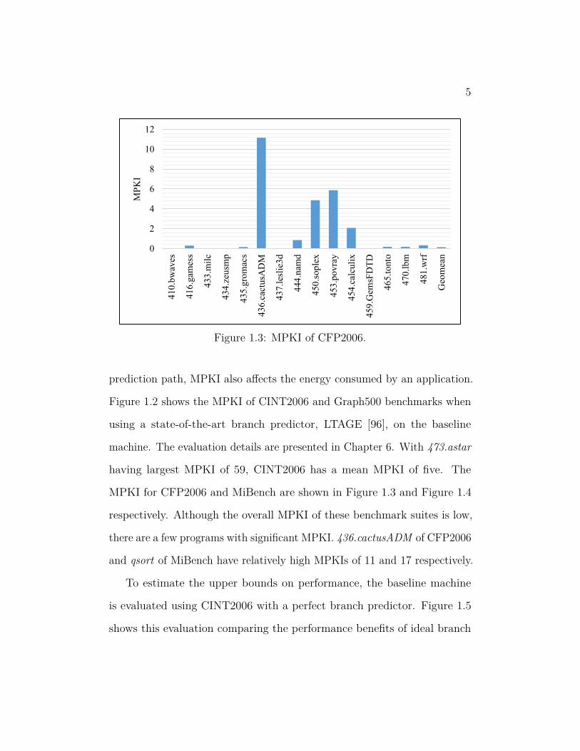
Figure 1.3: MPKI of CFP2006.
prediction path, MPKI also affects the energy consumed by an application.
Figure 1.2 shows the MPKI of CINT2006 and Graph500 benchmarks when
using a state-of-the-art branch predictor, LTAGE [96], on the baseline
machine. The evaluation details are presented in Chapter 6. With 473.astar
having largest MPKI of 59, CINT2006 has a mean MPKI of five. The
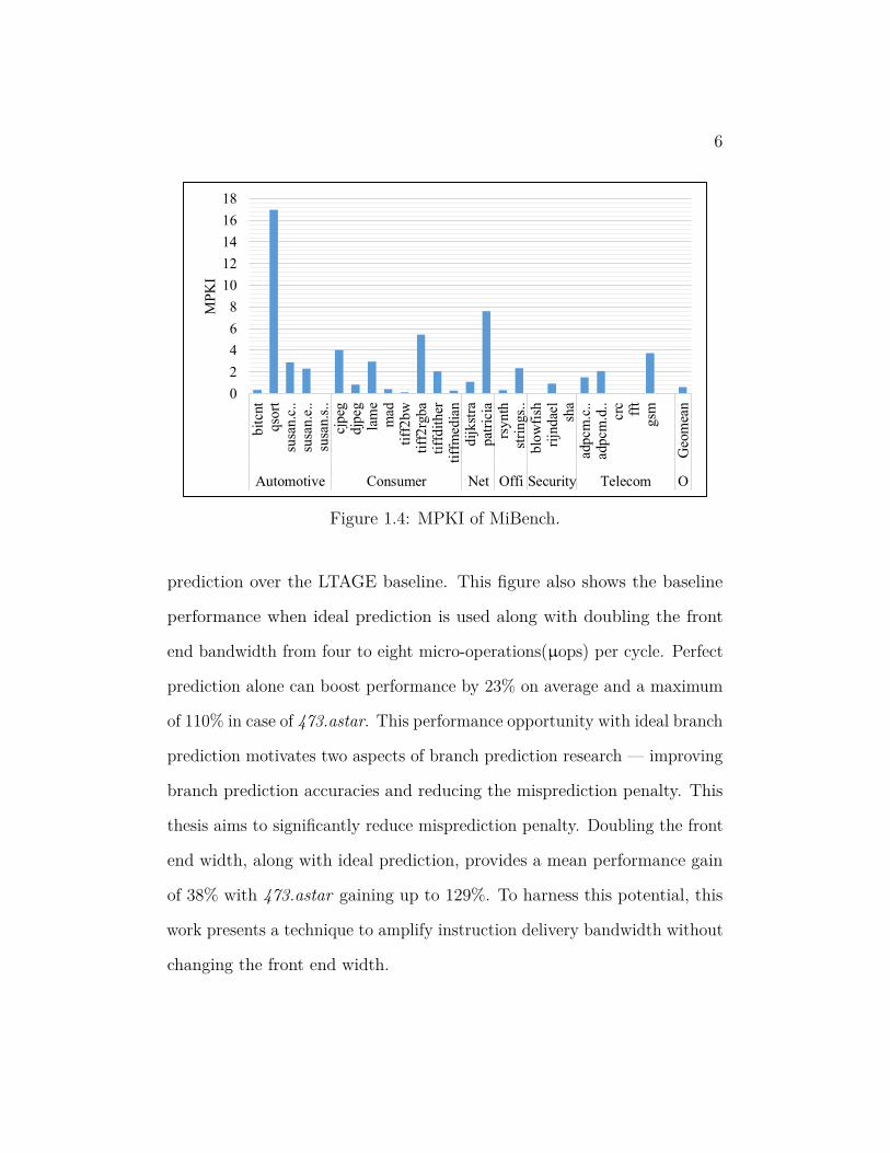
MPKI for CFP2006 and MiBench are shown in Figure 1.3 and Figure 1.4
respectively. Although the overall MPKI of these benchmark suites is low,
there are a few programs with significant MPKI. 436.cactusADM of CFP2006
and qsort of MiBench have relatively high MPKIs of 11 and 17 respectively.
To estimate the upper bounds on performance, the baseline machine
is evaluated using CINT2006 with a perfect branch predictor. Figure 1.5
shows this evaluation comparing the performance benefits of ideal branch
6
0
2
4
6
8
10
12
14
16
18
bit
cnt
qso
rtsu
san.c
..su
san.e
..su
san.s
..cj
peg
djp
egla
me
mad
tiff
2bw
tiff
2rg
ba
tiff
dit
her
tiff
med
ian
dij
kst
rapat
rici
ars
ynth
stri
ng
s..
blo
wfi
shri
jndae
lsh
aad
pcm
.c..
adp
cm.d
..cr
cff
tgsm
Geo
mea
n
Automotive Consumer Net Offi Security Telecom O
MP
KI
Figure 1.4: MPKI of MiBench.
prediction over the LTAGE baseline. This figure also shows the baseline
performance when ideal prediction is used along with doubling the front
end bandwidth from four to eight micro-operations(µops) per cycle. Perfect
prediction alone can boost performance by 23% on average and a maximum
of 110% in case of 473.astar. This performance opportunity with ideal branch
prediction motivates two aspects of branch prediction research — improving
branch prediction accuracies and reducing the misprediction penalty. This
thesis aims to significantly reduce misprediction penalty. Doubling the front
end width, along with ideal prediction, provides a mean performance gain
of 38% with 473.astar gaining up to 129%. To harness this potential, this
work presents a technique to amplify instruction delivery bandwidth without
changing the front end width.

7
0.0
0.5
1.0
1.5
2.0
2.5
3.0
3.5
4.0
4.5
400
.per
lben
ch
401
.bzi
p2
403
.gcc
429
.mcf
445
.gob
mk
456
.hm
mer
458
.sje
ng
462
.lib
quan
tum
464
.h26
4re
f
471
.om
net
pp
473
.ast
ar
483
.xal
ancb
mk
Geo
mea
n
IPC
LTAGE Ideal Ideal_X2
Figure 1.5: Performance effects of Ideal branch prediction and doubling thefront end bandwidth (_X2).
When a branch mispredicts, the misprediction penalty can be attributed
to execution-resume (ER) delay, and lack of mechanisms for capturing
control independence. ER delay is the elapsed time between resolution
of a mispredicted branch and start of execution of the first correct path
instruction. This delay depends on availability of instruction in various levels
of cache, but is typically equal to the front end delay, as most instructions
are found in either micro-operation cache(µop$) or level-1 instruction cache
(L1-I$). Control independence refers to reusing or reinstating younger
instructions that are beyond the control flow convergence point of the
mispredicted branch.
8
Conventional OoO
CRIB OoO
EMR OoO
BPred I$ VLDDeco-
de
Br
Check
Ren-
ame
µOp$Br
Check
Alloc Issue
RedirectR
edir
ect Fill Exec
Com-
mitPRF
BPred I$ VLD DecodeBranch
Check
Alloc
µOp$Branch
Check
CRIB
Exec
CRIB
Commit
Redirect
Red
irec
t
Fill
BPred I$ VLD DecodeBranch
CheckAlloc
EMR
Exec +
LOC$
EMR
Commit
ICU$Stall
RedirectF
ill
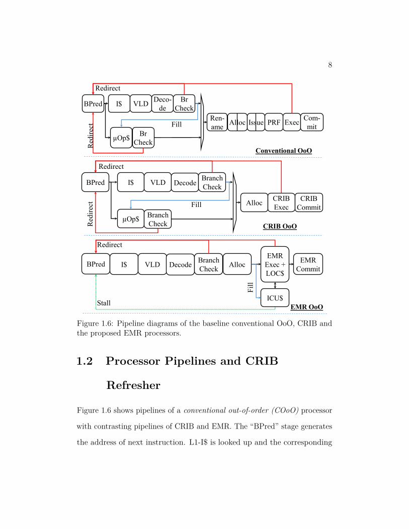
Figure 1.6: Pipeline diagrams of the baseline conventional OoO, CRIB andthe proposed EMR processors.
1.2 Processor Pipelines and CRIB
Refresher
Figure 1.6 shows pipelines of a conventional out-of-order (COoO) processor
with contrasting pipelines of CRIB and EMR. The “BPred” stage generates
the address of next instruction. L1-I$ is looked up and the corresponding
9
bytes are supplied to variable length decode(VLD) for demarcation. The
decode unit converts the instruction bytes into one or more µops. After
decoding the instructions, the “branch check” unit detects if the target
address of a direct-branch is mispredicted and redirects the front end to the
correct path.
A µop$, if present, is looked up in parallel with the L1-I$ look up. If the
target instruction is found in the µop$, then the L1-I$ data is ignored. The
set of micro-ops generated by the L1-I$ part of the pipe are added to the
µop$. Another branch checker is associated with the µop$ part of the pipe.
In a COoO, both L1-I$ and µop$ parts of the pipe merge and supply
instructions to rename stage where source registers are renamed to physical
registers using a rename table. These renamed instructions are allocated
mandatory resources like reorder buffer and issue queue entries, and optional
resources like destination physical registers and a load-store queue entry.
In the Figure 1.6, the rename and allocate units are assumed to take three
clock cycles and hence allocate unit is shown to take two clock cycles. The
issue unit can be divided into two pipe stages — “wakeup” and “select”. In
the “wakeup” stage, broadcast from instructions completed in this cycle is
used to identify dependent instructions that are ready to issue. From the
instructions that are ready to issue, instructions that can be issued in the
current cycle are selected in the “select” stage. The criteria for selection
depends on issue policy and resource limitation. The issued instructions
read the physical register file, execute, and after completion send a broadcast

10
Part 2
Part 1
Part 0
Part 3
Complex
Int
FPU
LSQ
Figure 1.7: Block diagram of CRIB.
signal to wake up dependent instructions. The completed instructions are
marked as such in the reorder buffer. Once the oldest instructions in the
reorder buffer completes, it is committed to the architectural state.
Figure 1.7 shows top level block diagram of CRIB. CRIB is an ELSE
machine where partitions consist of a limited number of program-ordered
instructions and dependencies within them are resolved through data flow.
Each partition consists of a designed number of execution stations each of
which holds one instruction. The interconnect between execution stations,
and between partitions communicate positionally correct values of all the
architectural registers. A ready bit is associated with each architectural
register which indicates the positional readiness of the register. When an

11
instruction is allocated into an execution station, the ready bit associated
with destination registers is cleared and set only when the instruction finishes
execution. This is used by the dependent instructions to determine if they
can start execution.
A set of latches at the head of each partition hold the architectural state
of the machine. These values are latched when the partition is promoted as
the architected partition, which indicates that the partition holds the oldest
set of instructions in the machine. Once all instructions in the architected
partition are completed, it commits and the next partition is promoted as
the architected partition.
Each execution station has a simple integer ALU, simple floating point
ALU and an address generation unit. Load store queue, integer multiply and
divide, floating point add, floating point multiply and other such complex
units are shared across multiple partitions to limit area and static power. As
shown in the Figure 1.6, CRIB consolidates the Rename, Issue and Execute
stages of COoO into one stage. Allocate stage is also simplified as only
execution stations are allocated to the instructions in this stage.
1.3 EMR Overview
Although EMR can be based on many ELSE machines or Revolver [35], this
thesis presents an implementation based on CRIB. The pipeline diagram
of EMR is shown in Figure 1.6. EMR has similar pipe stages as CRIB,

12
but enhances the Execute stages and repositions the µop cache to be more
effective. EMR introduces various novel techniques to increase application
performance while saving processor energy.
EMR introduces a novel instruction delivery mechanism called “In-place
fetch”. To implement In-place fetch, each CRIB partition is augmented
with a modest instruction memory, called location-optimized control cache
(LOC$), that stores multiple sets of instructions previously executed on
the corresponding partition. A control network is added between these
augmented partitions to communicate the address of next instruction. Using
the incoming instruction address, partitions can now select a set of instruc-
tions from this cache for execution. If the instruction corresponding to the
incoming address is not available in a partition, it can be serviced from a
special µop cache called In-core µop (ICU) cache.
ICU cache, which is structurally similar to the conventional µop cache, is
used to provide robust performance. This cache is located in the execution
core of EMR as seen from Figure 1.6 and is optimized as a backup cache
to furnish any capacity misses in the LOC$. Due to the usage model
and placement of the ICU$, instructions from this cache go through lower
number of pipe-stages than a conventional µop cache. This results in
faster instruction delivery to the execution core, than the conventional µop$.
Additionally, since ICU$ is only looked up when LOC$ misses, unlike the µop
cache that is accessed every active fetch cycle, it consumes lower energy than
the conventional µop$. If a required instruction is not found in the LOC$,
13
front end is redirected to supply this instruction to the back end. Using
novel techniques, instruction fetch requests are filtered to avoid redundant
and taxing front end redirects when the required instructions are already en
route.
On resolution of a mispredicted branch, the correct address of the next
instruction is passed to the next partition. When possible, the next partition
finds the target instruction using In-place fetch and quickly deliver the
correct path to the execution units. This dramatically reduces the execution
resume delay and speeds up the application. This novel recovery technique,
called “In-place Misprediction Recovery”, also performs selective recovery by
squashing only the instructions that are not control independent. Control
independent instructions are discovered by performing a simple look up in
an table that holds address of selected instructions in the EMR back end.
Once discovered, the intermediate partitions are forced to select No-ops to
allow propagation of correct architectural state to the partition with control
independent instructions.
1.4 Thesis Contributions
The key novel features of EMR are:
1. In-Place Fetch (IPF): A very small µop cache known as LOC$ is
added to each partition. When required, these caches can quickly
supply instructions to the execution stations.

14
2. In-Place Misprediction Recovery: On a branch mispredict, in-
stead of conventional squash recovery, EMR combines selective recovery
with IPF to perform an In-place misprediction recovery. When possi-
ble, the correct path instructions are delivered by the In-place fetch
instead of the front end. This results in reducing front end energy and
misprediction penalty.
3. In-Place Control Independence: EMR relies on CRIB’s data-flow
orientation to propagate branch targets in place, preventing control
independent instructions from being squashed and replayed.
4. Amplified Instruction Delivery (AID): Increasing the committed
partitions per cycle is easy in CRIB, but is not useful without increasing
front end bandwidth. In EMR, the combination of In-place fetch and
a speculative instruction selection amplifies number of instructions
delivered per cycle. AID boosts performance of many applications
even when the misprediction rates are low.
5. In-Core µop (ICU) cache: The ICU$ backs up the LOC caches
and provides robust performance. Due to its placement, instruction
delivery time to the execution core is significantly lower than the
conventional µop$. In addition, ICU$ also has lower accesses than the
traditional µop cache, resulting in lower energy consumption.
6. Filtered Demand Fetch: The EMR back end, which now is equipped
with a control network, often finds that the required instructions are

15
missing in the expected partitions. So, a necessary demand fetch unit
redirects front end to provide the required instructions. Novel filtering
mechanisms are employed to avoid redundant and taxing front end
redirects when the required instructions are already en route.
1.5 Thesis Organization
This thesis is organized as follows. Chapter 2 presents a review of prior work
in reducing misprediction penalties, and in ELSE architectures. Following
that, basics of EMR architecture are detailed in Chapter 3. Chapter 4
presents EMR enhancements to utilize control independence. Technique to
amplify instruction delivery with EMR is explained in Chapter 5. Apparatus
and methodology for evaluating EMR along with a detailed analysis of EMR’s
performance and energy are furnished in Chapter 6. Finally, Chapter 7
concludes this thesis with a summary of key concepts, observations and
possible related future work.
16
2 prior artA plethora of techniques have been proposed to reduce misprediction penal-
ties, mostly using control independence. Various ELSE machines have also
been proposed to address specific limitations of conventional out-of-order
processors. This chapter provides a detail overview of several related works
that have inspired the idea of EMR.
2.1 Background
The modern day processors are a result of a lot of innovation from many
researchers across the globe. In this section, a historical perspective of
processors and branch predictors is presented.
2.1.1 Instruction Level Parallelism
Instruction level parallelism (ILP) refers to the ability to process multiple
instructions at the same time. Higher utilization of ILP results in improved
performance of the applications.
Exploiting instruction level parallelism first started with pipelining the
processors back in 1950 [8, 54, 97, 99, 37, 112]. Pipelining allowed multiple
instructions going through various stages of processing. This increased the
throughput and operational frequency of computers.

17
The next epoch in computing has to be dynamic instruction scheduling.
Processors used the algorithm proposed by Tomasulo [119], later known
as Tomasulo’s algorithm, to dynamically generate instruction schedules [5]
and enable efficient utilization of resources. Later, superscalar processors
employed multiple ALUs and dynamic scheduling to improve performance
further [118, 94, 29, 78, 105, 107, 99]. Data parallel computing was another
important technique employed to improve performance [84, 91]. A single
instruction supplies the operation that has to be performed on multiple data
elements.
Till the introduction of out-of-order processing, instructions were sched-
uled for execution in the program order. Out-of-order processors identify
independent instructions in a finite instruction window and schedule them in
out-of-order fashion [82, 126, 51, 110, 55, 6, 32, 81, 99, 37, 112]. Exploiting
larger degree of instruction level parallelism and memory level parallelism,
these processors tend to have high performance and thus became popular
for commercial uses [28, 9, 102, 20, 33, 58, 50, 101, 34].
A different class of processors, called very long instruction word (VLIW)
processors, rely on compilers to specify parallelism [18, 90, 27, 45, 44, 22,
25, 24, 98]. Compilers can look at larger instruction windows to potentially
extract more parallelism. However, static scheduling can be limit the
opportunity due to dynamic control flow. The support from compilers
results in a simpler implementation and thus can be more energy efficient.

18
Control flow and data flow are two primary limitations to instruction
level parallelism. Data flow limitations refers to the restriction due to the
read-after-write, write-after-write and write-after-read dependencies on the
program instructions [99]. Read-after-write (RAW) is a true dependence that
will require the younger instruction to consume a value generated by the
older instruction. This will conventionally require the older instruction to
execute before the dependent younger instruction Rest are the dependencies
are commonly referred to as false dependencies.
Pipelining ALUs helps in executing multiple independent operations
in parallel. Register renaming in many out-of-order processors removes
the false dependencies by mapping the architectural registers to physical
registers or to reservation station entries [99]. Value prediction techniques
attack the true dependencies and exploit ILP beyond the data-flow limit [65,
64].
Control instructions like branch, call and return limit the ILP of a
program as these instructions can affect the consistent supply of instructions
by fetch unit to the rest of the pipeline [99]. Branch predictors are used to
circumvent these limitations on the ILP [114, 43]. The history and evolution
of branch predictors is presented in the next section.
2.1.2 Branch Predictors
Introduced in late 1960’s branch predictors were used to reduce interruptions
in instruction supply when a control instruction is encountered [19, 114,

19
43]. Later Smith presented dynamic branch prediction strategies which
could result in high prediction accuracies [106]. The bimodal predictor
proposed in this paper was used in many commercial processors [6, 110,
61]. While the bimodal predictor uses branch instruction address alone,
Yeh and Patt [127] propose inclusion of global branch history and local
histories in predicting branches. This two-level predictor improves prediction
accuracy by differentiating multiple instances of static branch by providing
context, and by correlating behaviour across multiple static branches. The
proposal in [127] also introduced the taxonomy of two-level branch predictors
depending on the possible combinations due to the types of branch history
registers, and the types of pattern history tables.
McFarling introduced a new way of looking up the branch predictors
using the XOR value of branch history register and the branch instruction
address [69]. The gshare branch predictor proposed in this paper was used in
IBM Power4 [116] and DEC Alpha 21264 [51]. Later, various hybrid predic-
tors were introduced by combining different types of branch predictors [10,
12, 76, 23]. Bi-Mode predictor introduced usage of two pattern history tables
and a choice predictor to reduce negative interference of branches in different
modes [59]. This predictor is used in the ARM A15 processor [57]. The
gskewed predictor proposed by Michaud et al., uses multiple pattern history
tables which are accessed using different hash functions [73]. The outcome
of the branch is determined by the majority vote of the predictions by these
history tables. Sprangle et al., proposed Agree predictor which uses the high

20
static predictability of branches and determines when to flip the prediction
outcome [111].
The YAGS predictor, introduced by Eden and Mudge, was derived from
bi-mode predictor, but introduced partial tags in the pattern history tables
to reduce negative interference [21]. Chang et al., introduced concept of
branch filtering by removing highly biased branches from the pattern history
table [11]. Alloyed history predictors, proposed by Skadron et al., fused
address of the branch instruction with local history and global history to
access the pattern history table [103].
Jimenez and Lin introduced perceptron branch predictor that computes
the outcome based on multiple weighted inputs [47, 48]. The perceptron
predictor learns that the correlations between the branch outcomes and uses
it to generate a prediction.
Overriding predictors use multiple predictors with ascending accuracies.
McFarling patented a predictor that uses a bimodal, local and global predic-
tor structures [68]. The bimodal predictor provides the default prediction for
every branch, but the local and global predictors have tag tables, similar to
ones proposed in [21], and provide predictions only when the tag matches in
their respective structures. The descending preference order of predictors is
global, local and bimodal. Michaud proposed a predictor that used multiple
tagged pattern history tables and used varying lengths of global history to
access different pattern history tables [72]. The pattern history table with
longest history that provides a prediction is used as the outcome. Seznec

21
proposed using geometric history lengths and other usability features to
further improve prediction accuracies [95, 96].
Instead of predicting the outcome of a branch, Jacobsen et al. proposed a
predictor to estimate the confidence of branch prediction [46]. This prediction
is useful in using control independence or to save energy by stalling fetch on
a low confidence estimation.
The target addresses of return instructions can be obtained by using a
return address stack [125, 49]. Due to out-of-order processing and precise
interrupts, the state of the return address stack can be corrupted and
Skadron et al. propose techniques to repair the same [104].
When an instruction is fetched, the target address is not known at least
till the branch instruction is decoded. In case of indirect branches, the
target address is available only after execution of the branch. Branch target
buffers are used to obtain the target address of the instructions at the fetch
stage [60].
2.2 Reducing Misprediction Penalty
The detrimental effect of traditional recovery from branch misprediction
is due to two primary reasons. First, all younger instructions are removed
from the machine and the front end has to fetch the correct path instruc-
tions. The delay in supplying the correct path instructions stalls execution
progress. Second, discarding these younger instructions that may have
22
already executed results in wasted work. Larger instruction windows and
deeper pipelines exacerbate the misprediction penalties.
2.2.1 Dual Path Execution
Multipath execution [36, 52, 124, 2, 120, 53] reduces misprediction penalties,
but can decrease performance and increases power consumption when both
paths of a correctly predicted branch are fetched/executed. Predication is
another common technique to avoid branches, but consumes excess resources
by fetching and executing multiple paths. Additionally, the forwarding of
correct speculative values outside of predicated blocks is delayed and can
affect performance.
2.2.2 Predication
Predication or Predicated execution is a technique to reduce short, hard-
to-predict branches. The boolean source operand, called predicate, is used
to conditionally execute an instruction [66, 42, 85]. It can be viewed as
software version of multi-path execution. While predication can prevent
mispredictions due to hard-to-predict branches, it can hurt performance
due to increased data dependencies. The multiple definition of a register
values which exist due to predication are partially addressed by predicting
the outcome of predicate and speculatively executing instructions dependent
instructions [17].

23
CI-1
?
CD-2 CD-1
CI-2
Y N
(a)
CI-1
?
CD-1
CI-2
Y N
(b)
Figure 2.1: Some examples of control independence.
Increasing accuracies of branch predictor and aggressive out-of-order
techniques discourage usage of predication in modern processors. This can
even be observed from the severe limitation on predication in new 64-bit
ARMv8 instruction set [63].
2.2.3 Control Independence
Control independence property stems from the observation that only a small
portion of code is dependent on the branch outcome. Often, after the short
control dependent path, the control flow of the program merges and executes
instructions irrespective of the branch outcome.
The control independence taxonomy [4] of instructions in the processor
pipeline, that are younger than the mispredicted branch is as follows:
24
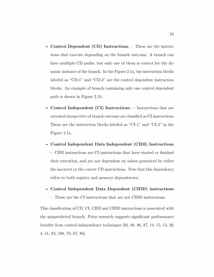
• Control Dependent (CD) Instructions — These are the instruc-
tions that execute depending on the branch outcome. A branch can
have multiple CD paths, but only one of them is correct for the dy-
namic instance of the branch. In the Figure 2.1a, the instruction blocks
labeled as “CD-1” and “CD-2” are the control dependent instruction
blocks. An example of branch containing only one control dependent
path is shown in Figure 2.1b.
• Control Independent (CI) Instructions — Instructions that are
executed irrespective of branch outcome are classified as CI instructions.
These are the instruction blocks labeled as “CI-1” and “CI-2” in the
Figure 2.1a.
• Control Independent Data Independent (CIDI) Instructions
— CIDI instructions are CI instructions that have started or finished
their execution, and are not dependent on values generated by either
the incorrect or the correct CD instructions. Note that this dependency
refers to both register and memory dependencies.
• Control Independent Data Dependent (CIDD) instructions
— These are the CI instructions that are not CIDD instructions.
This classification of CD, CI, CIDI and CIDD instructions is associated with
the mispredicted branch. Prior research suggests significant performance
benefits from control independence techniques [92, 88, 86, 87, 14, 15, 13, 26,
4, 41, 83, 108, 70, 67, 80].
25
CD-1
BR
CI
BR
Squ
ash
BR
CD-2
CIF
etch
& E
val
Squash Recovery
Br
CI
Squ
ash
Br
CI
CD-2
Fet
ch &
Eval
Sel
ecti
ve
Eval
Selective Recovery
Figure 2.2: Squash and selective misprediction recovery techniques.
In order to benefit from the control independence property, the following
steps are typically employed.
1. Selective Recovery: Figure 2.2 illustrates the difference between
squash and selective recoveries. Unlike squash recovery, which re-
moves all instructions younger than the mispredicted branch from the
machine, selective recovery removes only CD instructions from the
machine. The convergence point, usually provided by a predictor, is
used to stop instruction squashing.
2. Smart Fetch Redirect: After selective recovery, FE is redirected
to bring the correct CD path instructions into the machine. When

26
CI instruction fetch is detected, FE is redirected to resume fetching
instructions from the end of CI path.
3. Dependency Fix: After selectively removing incorrect CD instruc-
tions and inserting correct CD instructions, register and memory
dependences have to be fixed to supply correct operands to CI path.
This, typically, is a tedious task and various approaches have been
used in prior proposals.
Lam and Wilson published the seminal work on control flow limitations
on parallelism where they identified control independence [56]. The first
processor to utilize control independence was the Multiscalar processors [109]
which is described further in Section 2.3.1.
In trace processors [89, 122], dynamic instruction stream is divided into
frequently executed sequences called “traces”. After squashing the trace
containing a mispredicted branch, other traces selectively squashed till the
new set of traces are already present in the processing elements.
Sodani and Sohi propose instruction reuse buffer [108] as a way to exploit
control independence. The outputs of an instruction corresponding to its
inputs are recorded in a buffer. If a recurring instruction, looked up using
inputs, has an entry in the reuse buffer, the output results are reused from
the buffer instead of computing them again. On a resolving a mispredicted
branch address, all the younger instructions are removed from the machine.
27
However, due to source equivalence check, control independent instructions
with unchanged input operands will not re-execute.
Rotenberg and Smith [88] augment the ISA to encode the branch conver-
gence point, so that software can furnish it. CIDI instructions are determined
by source equivalence check similar to the instruction reuse proposal [108].
Selective branch recovery [26] uses control independence of if-then type
branches only by using a recovery buffer suggested in [3].
In Transparent Control Independence [4], Al-Zawawi et al. execution of
CIDI instructions is decoupled from the CD and CIDD instructions when
executing the predicted path of a branch. A structure called the re-execution
buffer or RXB in short, is used to store the CIDD instructions along with a
copy of their source values that are generated by a CIDI instruction. After
a branch misprediction is resolved and the correct CD path is inserted into
the machine, the self-sufficient recovery program in the RXB is inserted into
the machine.
Hilton and Roth proposed Ginger [41], which uses register tags to track
CIDI instructions and fix dependences for CIDD instructions. A register
tag search-and-replace operation is done on the CI path. The replaced tag
is obtained from the check-pointed rename map which was captured after
the incorrect CD path. The current rename map provides the replacer tag.
Some proposals for control independence rely on squash recovery instead
of selective recovery [15, 13, 83, 108]. Chou et al. propose to defer execution
of the CD path of a hard-to-predict branch till the branch’s direction

28
is resolved [15]. Skipper [13], proposed by Cher and Vijaykumar uses a
similar technique. A predictor is trained to gather information about the
predictability of a branch, its convergence point, resource consumption of
its possible CD paths and its CIDI instructions. After fetching a branch
of interest, FE uses this predictor information to skip ahead to fetch and
execute the CIDI instructions. Sufficient resources are reserved for the CD
path during this out-of-order fetch process.
In SYRANT [83], Premillieu and Seznec suggest that, when CI instruc-
tions are fetched again, they are allocated with the same physical register,
LSQ entry and ROB entry as they were in the first instance. Since the
results of a CIDI instruction are already preserved in the their destination
register, these instructions complete immediately.
To summarize, numerous proposals have identified the importance of
decreasing branch misprediction penalty. Proposals like dual path execution,
eager execution and predication increase energy consumption and can poten-
tially hurt performance when branches are predictable. Utilizing the control
independence property shows significant potential, but previous proposals
have been limited in either usage or implementability. This dissertation
derives concepts from these prior proposals to formulate a practical processor
that minimizes misprediction penalty significantly.

29
2.3 Execution Localized Scheduling Engines
A study of processor evolution reveals the design choices followed by modern
processors. Originating from an era with expensive logic components, simple
multi-cycle processors evolved into pipelined scalar cores. As the logic
component cost decreased, processors evolved from in-order scalar processors
to in-order superscalar processors and now into wide-issue out-of-order
processors. In the modern processor, reservation station, bypass network,
physical register files, reorder buffer, checkpoint tables and load-store queues
are required to support the wide-issue and out-of-order techniques to achieve
higher performance. However, there are other ways of achieving wide-issue
and out-of-order processing which do not need most of these units. Starting
from a new base, ELSE machines have some very lucrative features with
feasible challenges.
Many ELSEs have been proposed in the past to address the scalability
of conventional out-of-order processors. These proposed ELSE machines
share some basic features.
1. Processing elements or cores, that execute all operations, are replicated.
2. Each processing element has a localized instruction scheduling logic.
3. Processing elements communicate data and control via an intercon-
nection network.

30
Details of Multiscalar [109], RAW [115], TRIPS [93], Ultrascalar [39],
LEVO [121] and CRIB [30] are discussed in this section.
2.3.1 Multiscalar
Multiscalar [109], proposed by Sohi, Breach and Vijaykumar, is designed to
extract large quantities of instruction-level parallelism from single-threaded
programs. A single-thread program is divided into multiple tasks where,
each task can contain multiple instructions corresponding to a contiguous
regions of the program’s control flow graph. These tasks, which need not be
fully independent, are distributed across various scalar cores to be executed
in parallel. The abstract unified logical register and sharing of the memory
dependence unit across all the scalar cores resolves dependences across tasks.
In Multiscalar, the scalar cores are connected using a unidirectional ring
network. Dependency resolution are communicated using the ring network
and is orchestrated by the compiler. When all the instructions of a task
complete, the corresponding core commits by advancing the commit pointer
to the next scalar core on the ring network.
This architectural paradigm provides many benefits over traditional
processor architectures.
• Due to the task-oriented structure, Multiscalar processors can perform
selective branch prediction. As long as the global control flow is not
disturbed by a mispredicted branch, all tasks can keep executing in

31
parallel. A mispredicted branch within a task need not have any impact
on the global control flow and would not invalidate the younger program
tasks, which is a form of control independence [87]. This property
abates the branch misprediction penalty on Multiscalar processors.
• Multiscalar can effectively extract parallelism in much larger portions
of a program. While conventional processors use a limited size issue
queue to search for parallel instructions, Multiscalar has only a subset
of instructions per scalar core that are under consideration for execution
.
2.3.2 RAW
RAW [115], proposed by Taylor et al. is a tiled architecture with processor
tiles connected via a two-dimensional mesh network. Conventionally, the
inter-core communication is done via coherent memory interfaces, which
can have higher area, delay and energy costs. Inter-core communication is
exposed to the software by ISA extensions the expectation that compiler
driven inter-core communication will be more efficient and effective. Due to
reduced costs, hardware is expected to be more scalable.
The RAW processor has 16 cores connected using four 32-bit interconnec-
tion networks — two statically routed and two dynamically routed. Static
routing is configured by the compiler and dynamic routing is configured
at runtime. The ISA extensions expose these interconnection networks

32
by mapping them as “network registers” which are constructed as FIFO
queues. A platform specific compiler makes use of these operand networks
to distribute and coordinate work between multiple simple cores. Both
instruction-level and thread-level parallelism are explored in this work.
2.3.3 TRIPS
Sankaralingam et al. proposed TRIPS [93] processor that uses ISA extensions
to explicitly communicate data flow dependencies between the processing
tiles. There are 16 processing tiles interconnected via a single cycle inter-
connection. The compiler generates 128-instruction blocks and distributes
them as group of eight instructions across the 16 tiles. Since the compiler
has complete control on the placement of instructions within the instruction
tiles, any exposed communication latencies can be minimized. However,
interconnection latencies still have significant effect on the performance of
TRIPS machines.
2.3.4 LEVO
Uht proposed a general purpose out-of-order ELSE machine called LEVO [121]
which does not need any specific compiler support for its operation. This
machine enables use of aggressive speculative techniques like disjoint eager
execution and hardware-based predication to extract maximum instruction
level parallelism. LEVO has a scalable resource flow execution model and is

33
implemented using an execution window that is organized as a matrix of
“Active Stations” that hold instructions. Instructions are committed as one
Active Station column at a time after all instructions in that column have
finished execution.
Multiple Active Stations, referred to as “sharing group”, can share a
processing element that can perform all the operations required by the ISA.
A sharing group also shares a set of buses, called spanning buses, that carry
packets consisting of time-tag, address and data corresponding to a register.
These spanning buses are used by the active stations to obtain the source
register values and to drive the destination register values. Full values of
specific architectural registers are stored at the end of each sharing group to
provide any register values to the next sharing group. Buses in the reverse
direction can be used by the active stations to request values of registers
that are no longer broadcast actively.
LEVO does not have any explicitly defined set of architectural register
file. All operands are communicated via the spanning buses and time-tags.
Time-tags are associated with all the register values broadcast on the buses.
Time-tags are used by the Active Stations to grab the youngest of the older
values of source registers from the spanning buses. To perform this each
Active Station has comparators to match the register address and time-tags
begin broadcast on the spanning buses. Every time an Active-Station grabs
a older register value that is not older than the current captured value, it
requests for and, if granted, triggers execution of that instruction.

34
LEVO also performs full explicit predication conversion of branches
if the branch target is already in the machine. After an eligible branch
is determined, the fetch logic brings instructions according to the actual
instruction layout in the memory and associates predicate bits to these
instructions in hardware. Disjoint eager execution [120], where both paths
of a branch can be executed before a branch actually resolved, is also
implemented in LEVO. In their evaluation, the authors found that scaling up
the instruction window sizes results in committing more than ten instructions
per clock.
2.3.5 Ultrascalar
Ultrascalar processor [39], proposed by Henry, Kaszmaul and Viswanath,
aims to dramatically reduce the asymptotic critical-path length of a super-
scalar processor from O(n2) to O(logn). The processor is implemented as
a large collection of execution stations, each of which contains an ALU and
a router. These execution stations are connected by a network of parallel-
prefix tree circuits. Allocated in program order, these networks provide
full functionality of superscalar execution including renaming, out-of-order
execution and speculative execution. When scaled up, ultrascalar is limited
by the network and latch delays to effectively awaken dependent instructions
that are far in program order.

35
Part 2
Part 1
Part 0
Part 3
Complex
Int
FPU
LSQ
Figure 2.3: Top level view of CRIB unit.
2.4 CRIB
CRIB [30], proposed by Gunadi and Lipasti, is an ELSE machine where
partitions consist of a limited number of program-ordered instructions and
dependencies within them are resolved through data flow. The partitions
themselves are connected to each other using a unidirectional ring network
that carries positionally correct values of all architected registers. Each
partition consist of a fixed set of execution stations where each execution
station can execute one instruction.
As shown in Figure 1.6, CRIB uses the same fetch and decode units as
a conventional out-of-order. The Allocate unit bundles instructions into

36
ES 0
ES 1
ES 2
ES 3
R0, R1, … … R7
R0, R1, … … R7
Part
itio
n
Inst 3
Inst 2
Inst 1
Inst 0
Figure 2.4: Internals of a CRIB partition.
groups and assigns them to an appropriate partition, if it is available. The
rename table, reservation station, ALU, bypass network and the reorder
buffer are consolidated into a single structure called execution station (ES).
Physical register file is decentralized into sets of register latches at the head
of each partition.
Figure 2.3 shows the top level organization of of CRIB’s back-end, also
referred to as the execution-core. The execution core consists of multiple
partitions connected and managed in a circular queue fashion. Each partition,
as shown in Figure 2.4, consists of multiple ESs and the instruction bundle
allocated to the partition supply instructions for each ES. Each ES has
multiplexers to select the source operands, an ALU to perform operations on
these operands and an output router to drive the generated result. Internals
of an execution station are illustrated in Figure 2.5. When an instruction is
37
R0, R1, … … R7 R0, R1, … … R7
ALU
Done
Compute
R0, R1, … … R7
Input Select
Operation
Select
Output
Select
Done Exec
uti
on
Sta
tio
n
Figure 2.5: Internals of a CRIB execution station.
portioned to an ES, the Done bit is cleared and the input multiplexers, ALU
and output router are configured accordingly. This done bit is set when the
allotted instruction finishes execution. The interconnect carries full value
and the readiness of all the architecturally visible registers.
Each incoming and outgoing register lanes have a ready bit that indicates
the spatial readiness of the architectural register. Each ES drives ready
bit of the allocated instruction’s destination register using the Done bit.
Dependence resolution is done by using the spatial readiness of architectural
registers. Instruction starts executing as soon as all the incoming register
sources are ready. After the execution is complete, the done bit of the
ES is set and the new destination values are propagated out. Dependent

38
instructions, subject to the readiness of other sources, may wakeup and
start execution using this newly generated operand. Since independent
instructions may have all their sources ready at the same time, they can
execute in out-of-order fashion.
When all the ESs have finished execution, the partition is ready to
commit. An architected partition holds the oldest instruction bundle in the
machine and since Commit is done in program order, only the architected
partition is eligible for Commit. When committing a partition, the LSQ
resources allocated to it are reclaimed and the next partition is made as the
architected partition. As a partition is promoted to architected partition
state, the set of register latches, present at the input of this partition, are
made opaque and block all incoming propagations on the interconnect.
Complex structures like multipliers, floating point units, load store
queues or any other units that are expensive are shared by all the CRIB
partitions. Request queues allow data transfer between these shared units
and execution. Squash recovery is implemented by a signal from mispredicted
ES and invalidation of the younger ES. On receiving the invalidate signal,
ES releases any held resources, like the LSQ entries. Exception recovery is
complete as the Allocate unit resets the allocating partition to the partition
following the mispredicted partition.
In CRIB, LSQ entries are requested and assigned at execution time, after
the address of a load or store is complete. This significantly reduces the de-
sign size of the LSQ. In addition to the ready signal, each architected register
39
0.00
0.50
1.00
1.50
2.00
2.50
3.00
3.50
4.00
400
.per
lben
ch
401
.bzi
p2
403
.gcc
429
.mcf
445
.gob
mk
456
.hm
mer
458
.sje
ng
462
.lib
quan
tum
464
.h26
4re
f
471
.om
net
pp
473
.ast
ar
483
.xal
ancb
mk
Geo
mea
n
seq
-csr
seq
-lis
t
CINT2006 Graph500
IPC
Conv.OoO192
CRIB64
Figure 2.6: Comparison of baselines: Performance of CRIB with 64-entrywindow is compared to a convention out-of-order processor with 192-entrywindow.
propagation on the interconnect carries a re-execute signal. While cleared
on allocating an instruction, this bit is set by mispredicted loads to enable
dependent instructions to just re-execute instead of performing a squash
recovery. So simple, yet aggressive memory-disambiguation techniques can
be used.
Figure 2.6 shows the instructions-per-clock (IPC) of the baseline 64-
entry CRIB and the baseline 192-entry conventional out-of-order. Table 6.1
provides configuration details for these processors. This figure is intended
to present an idea of EMR performance comparisons with CRIB baseline

40
and not to analyze various contributing factors of CRIB’s performance —
which is throughly done in [30].
In this dissertation, the implementation of CRIB differs from the proposed
and evaluated model in [30]. A µop cache is added to make CRIB as a
comparable baseline. Considering the process improvements from 65nm to
22nm, larger instruction window CRIB is also assumed.
2.5 Summary
This chapter presented a large subset of prior work related to the main
proposal of this thesis. Previously published work in branch misprediction
penalty reduction has been explored, with a special emphasis on control in-
dependence techniques. Alternate implementations of out-of-order machines,
that fall into the ELSE category, were studied. The CRIB microarchitecture
is explained in detail to help some of the fundamentals of the proposed EMR
architecture.

41
3 express misprediction
recoveryThis thesis work is on reducing the misprediction penalty of branches by
using architectural enhancements to CRIB microarchitecture. Depending on
the criticality, architectural components of express misprediction recovery
(EMR) are segregated into core concepts and enhancements. Core concepts
of EMR are detailed in this chapter and enhancements to EMR are presented
in later chapters.
3.1 Motivating Example
EMR augments each CRIB execution partition with a localized instruction
cache(LOC$) that holds multiple instruction bundles. As the Allocate unit
inserts instruction bundles into appropriate partitions, branch instructions
along with their predicted control paths are cached in this local storage.
When a mispredicted branch completes execution, the resolved address is
sent to the next partition via the newly added control network. If the
instruction bundle corresponding to the incoming address is found in the
local instruction store of the next partition, it is selected for execution. In
steady state, these LOC$ hits are likely, which can dramatically reduce the
misprediction penalty.

42
Example Code
L3 R4 M[R0]
CMPS R4, 0
BEQ L1
R1 R1 + 1
JMP L2
L1 R2 R2 + 1
L2 R0 R0 + 1
CMPS R0, R3
BLT L3
(a) Example
LATCH
[Arch] LATCH
R4 M[R0]
CMPS R4, 0
BEQ L1
R1 R1 + 1
JMP L2
R0 R0 + 1
CMPS R0, R3
BLT L3
Par
titi
on
-0P
arti
tion
-1
LOC$
LOC$
(b) Predicted path executionand branch resolution
R2 R2 + 1
LATCH
[Arch] LATCH
R4 M[R0]
CMPS R4, 0
BEQ L1
No Op
R0 R0 + 1
CMPS R0, R3
BLT L3
Par
titi
on
-0P
arti
tion
-1
LOC$
LOC$
(c) Recovering from mispre-dict
Figure 3.1: Example illustrating basic EMR functionality. The branch withL1 as the target is the mispredicted branch.
As an example, consider steady-state execution of the loop presented in
Figure 3.1a which has a branch, BEQ L1, that is hard to predict. Assume
that in this iteration, the branch was predicted as "not-taken" and the
execution in a two-partition EMR is as shown in Figure 3.1b. This figure
shows the localized storage at the execution station (ES) level to improve
comprehensibility of the example. Now when the branch resolves as "taken",
partition-0 sends out address L1 as the input instruction address for partition-
1. As shown in Figure 3.1c, due to steady-state assumption, partition-1
finds this instruction bundle in the localized cache, selects and starts its
execution, thus reducing the ER delay. The instructions in ES1, ES2 and
43
ES3 of partition-1 are CIDI instructions that may have finished execution
and will not re-execute to further improve performance.
In general, when a mispredicted branch resolves, the correct path, if
cached, is selected in the subsequent partitions. During this selection process,
if control independent instructions are found, control independence is utilized
by avoiding re-execution the CIDI instructions and quickly commiting such
instructions when possible.
3.2 Architectural Overview
EMR enhances CRIB by introducing new architectural components to
implement the target functionality. This section presents an overview of
new architectural components in EMR.
Figure 3.2 shows the top level diagram of EMR. Each partition gains a
partition control unit(PCU) that coordinates program control with adjacent
PCUs via the newly added control interconnect. When required, a PCU
can also request for specific instructions to be fetched and allocated into
its corresponding partition. A demand fetch unit, marked as FE DF in
the Figure 3.2, is used to aggregate the requests from all the PCUs, and
redirects the front-end only when required. The PCU and demand Fetch
units are further discussed in the future sections of this chapter. A local
sequence number (LSN) that corresponds to program order is assigned to

44
Part
0
Part
1
Part
2
Part
3
PCU
PCU
PCU
PCU
FE
DF
Complex
Int
FPU
LSQ
To
Fetch
Figure 3.2: Overview of EMR architecture.
Inst. address µOp Number Valid BMP token
Figure 3.3: Control communication between the partition control unit.
each instruction instance in an ES. The LSN is used to prioritize fetch
requests, and to order memory operations correctly.
As shown in the Figure 3.3, the interconnect between the PCUs carries
four different components. Instruction Address is used to communicate
the address of next instruction from one PCU to another. Some instructions
have multiple µops and µop Number communicates the µop number of the
next instruction. A Valid bit signifies the validity of the incoming address
and enables different actions in the destination PCU.
45
LOC$Select
PropagateFE Com
PCU
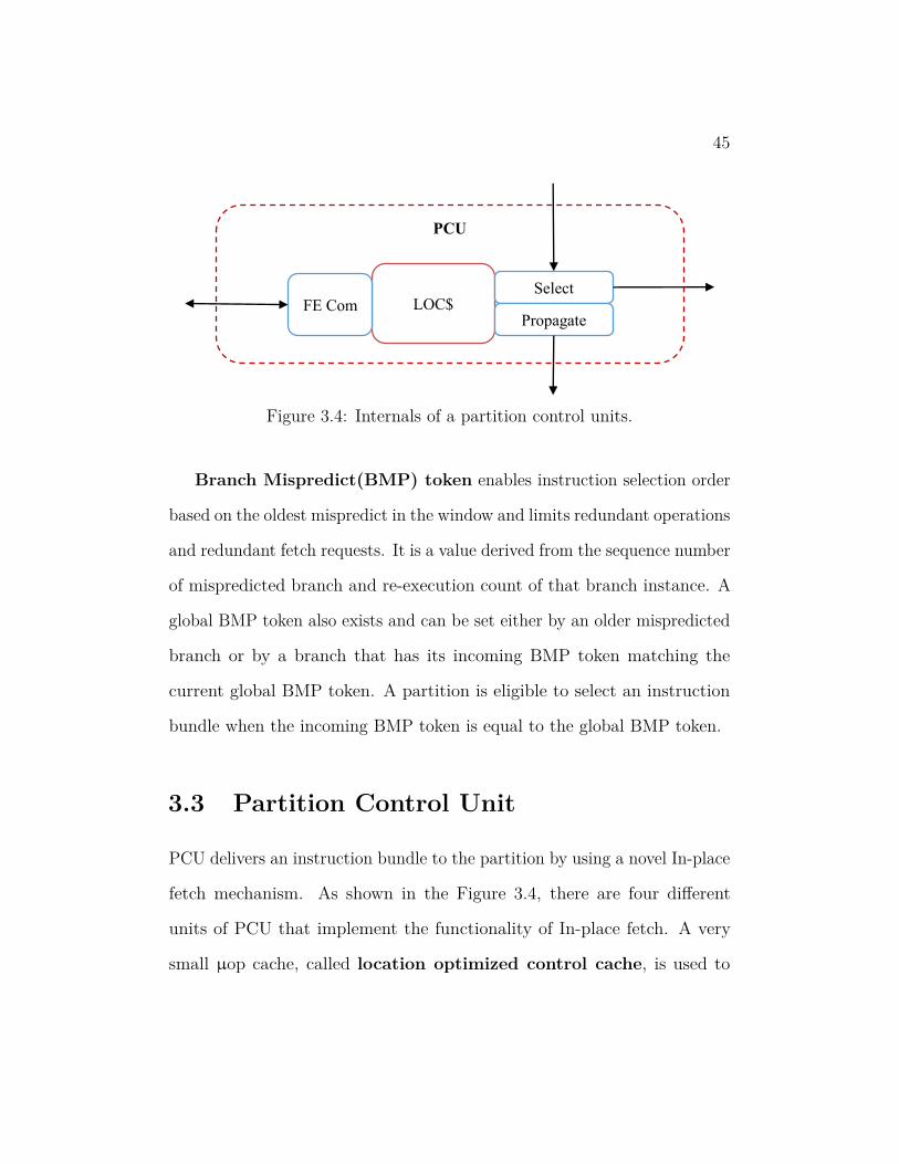
Figure 3.4: Internals of a partition control units.
Branch Mispredict(BMP) token enables instruction selection order
based on the oldest mispredict in the window and limits redundant operations
and redundant fetch requests. It is a value derived from the sequence number
of mispredicted branch and re-execution count of that branch instance. A
global BMP token also exists and can be set either by an older mispredicted
branch or by a branch that has its incoming BMP token matching the
current global BMP token. A partition is eligible to select an instruction
bundle when the incoming BMP token is equal to the global BMP token.
3.3 Partition Control Unit
PCU delivers an instruction bundle to the partition by using a novel In-place
fetch mechanism. As shown in the Figure 3.4, there are four different
units of PCU that implement the functionality of In-place fetch. A very
small µop cache, called location optimized control cache, is used to

46
store a trace of instruction bundles previously executed on the associated
partition. Based on the incoming address, the select unit looks up the
location optimized control cache and supplies instructions for execution.
The propagate unit generates the address of next instruction bundle based
on the incoming address. If an instruction bundle was not found in the
location optimized cache, the select unit generates a fetch request. This
fetch request is communicated to the demand fetch unit by the front end
communication interface.
3.3.1 Location Optimized Control Cache (LOC$):
LOC$ is envisioned as a small, associative µop cache that is written when
instruction bundles are allocated to the partition. This cache is envisioned
to typically hold four to 16 instruction bundles. Each entry is tagged by the
address of the first instruction in the instruction bundle.
As the name suggests, LOC$ is optimized for locality. Multiple LOC
caches are allowed to replicate instructions to quickly provide them to their
respective partitions. An alternative solution is to route the control path
back to the partition containing the required instructions. Such a solution
is most likely to increase the no-op filled partitions which can severely affect
performance due to decreased effective instruction window size.
The usage of LOC$ is a bit different than the normal caches. Normally,
a cache is looked up for an entry and data is filled into the cache only when
it is not present. In case of LOC$, instruction bundles can be speculatively

47
allocated which can result in multiple instances of an instruction bundle in a
LOC$. This lowers the effective capacity of a cache and is very undesirable.
Replication in the LOC$ can be avoided by checking if an instruction bundle
is already present in the LOC$ before inserting it. This requires a look up
preceding every write, which increases power consumption and, in some
cases, increases instruction delivery delay.
EMR employs three preventive measures to keep the power and delay in
check. First, the back end of EMR is conservatively marked as full when the
allocation pointer reaches the commit pointer. A more aggressive allocation
would have proceeded to allocate till all the LOC caches are full. This
conservative approach dramatically reduces LOC$ pollution and replication
while saving power. Second, each partition is provisioned with a separate
single-entry cache line, called fill buffer, that holds the allocated instructions.
When a partition needs to select an instruction bundle, both LOC$ and
the fill buffer are looked up. If the fill buffer has the instruction, its entries
are supplied for execution. Finally, the LOC$ is written with the entries
supplied for execution by the fill buffer, only if the LOC$ did not have
the corresponding instruction bundle. These three techniques increase the
effective capacity of the LOC caches. LOC$ replacement is managed by
pseudo-LRU policy.

48
3.3.2 Select Unit:
This unit performs an associative look up of the LOC$ using the incoming
instruction address and delivers the instruction bundle to the partition. If
the instruction bundle is not found in LOC$, this unit initiates a fetch
request by using the front end communication interface.
3.3.3 Propagate Unit:
Based on the incoming address and the type of instruction, this unit generates
the next instruction address, similar to the next address generator in the fetch
unit. When front end is turned off, this unit can use the branch predictor
to predict the outcome of branches supplied by the LOC$. Additional
discussion on branch prediction is presented in Section 3.5.
3.3.4 Front End Communication Interface:
On receiving a fetch request from the Select unit, this unit appends the
partition number and the LSN of the first ES to the received fetch request
before sending it to the demand fetch unit. Since only one instruction fetch
request is valid at a given time, the fetch communication interface could
interface with the demand fetch unit using a bus that is shared between
many PCUs. Bus master prioritization can be easily done on the basis of
the LSN of the requester.

49
ICU$FR FSM ArbTo
Fetch
Front-End Demand Fetch (FEDF)
Figure 3.5: Components of demand fetch unit.
3.4 Demand Fetch
If a target instruction bundle is not found in the LOC$, due to either a cold
or conflict miss, a request is placed with the demand fetch unit which selects
and services the oldest fetch request. Figure 3.5 presents the internals of the
demand fetch unit, which has three main sub-units. In presence of multiple
fetch requests, the Request Arbiter selects the fetch request with lowest
LSN. To reduce front end redirects, the oldest fetch request can be sent to
front end redirect unit only after determining that ICU$ can not service
the request. However, such serial process increases cycle count required for
front end redirect and can impede or even hurt performance. In order to
minimize the service delay, the oldest request is simultaneously sent to both
ICU$ and the front end redirect unit.
50
3.4.1 In-Core µop (ICU) Cache:
This cache is structurally similar to the µop cache in the baseline CRIB, but
supports both demand fetch, and speculative push to the LOC$. The selected
request from the arbiter looks up the ICU$ for the required instruction
bundle. If found, the request is serviced by the ICU$ and any front end
fetch triggers made simultaneously are cancelled. The serviced instruction
bundle is inserted into the requested partition.
In an effort to reduce the number of fetch requests, the ICU$ also
speculatively pushes subsequent instruction bundles in the following cycles.
Pushes continue till either a branch is encountered in the supplied stream or
the target bundle is not found in ICU$. These pushed instruction bundles
are inserted into LOC caches in consecutive partitions. The ICU$ and the
baseline µop cache are eight-way set-associative, managed with pseudo-LRU,
and hold an instruction bundle in every way of every set.
Since ICU$ is also a back end cache like LOC$, instruction bundles
can be inserted even when they are already present in the cache. Special
insertion policies are warranted to minimize data replication and maximize
effective cache capacity. Instruction bundles are looked up for presence
before insertion. Since ICU$ is written when it is not servicing any fetch
requests, delayed writes do not affect performance. Given that the number
of fetched instructions is low in most benchmarks, the energy increase due
to the additional look ups is lower. Since LOC and ICU caches are now

51
Idle
Normal
Service
Init
ial
Fet
chTrigger Fetch
Cancel Service
Forc
e F
etch
Tri
gger
Figure 3.6: Finite state machine at the demand fetch unit that indicatesthe state of the front-end.
present in the back end of the pipeline, they are henceforth also referred to
as back end caches.
3.4.2 Front End Redirect:
This unit uses a finite state machine (FSM) and fetch filtering to determine
when to redirect the front end. The FSM, illustrated in Figure 3.6, has three
states reflecting the status of the front end — Idle, Service and Normal.
When the FSM is in the “Idle” state, the front end is turned off. Front
end is is active in the other two states of the FSM. “Idle” on reset, the
initial fetch transitions the FSM to “Normal” state. In “Normal” state,
52
the front end is supplying instructions to the execution core, just like in
the traditional instruction delivery mechanism in baseline conventional
out-of-order processor and CRIB. If in “Idle” mode, a fetch request from
the request arbiter can trigger transitions of the FSM to “Service” state and
the front end will be redirected.
In “Service” mode, the front end is expected to deliver the instructions
that were not found in the back end caches (LOC and ICU caches). A
record of the fetch request, that is currently under service, is maintained to
allocate the requested instruction bundle to the requested partition. The
FSM transitions to the “Normal” state as soon as the first instruction
bundle corresponding to the requested address is allocated. A fetch request,
currently under service, could be cancelled due to a ICU$ hit or due to an
older branch mispredict. In such cases, the FSM goes into the Idle mode till
a new fetch request is made. An older fetch request can override the fetch
request that is currently under service. If requested address is different, a
new redirection of the front end is triggered. Otherwise, the information
about requested partition is updated in the service record.
After reaching a threshold number of LOC$ hits for the allocated instruc-
tion bundles, the front end can be turned off to save energy. In this case,
the FSM transitions from “Normal” state to “Idle” state. Typically, fetch
requests that occur during “Normal” state are ignored with an assumption
that the requested instructions are en route and may be delayed due to
the front end latencies. However, some fetch requests can force the FSM

53
to change from “Normal” to “Service” state when the front end is not
fetching the requested instructions. This happens when a mispredicted
branch provided by front end, finds part of correct path in LOC caches
and the front end continues to fetch from an incorrect path. To detect
this scenarios, a front end address table (FEAT) is used to maintain the
addresses of instructions in flight in the front end.
FEAT can be looked up associatively to determine if the requested
address is already en route. If not, the FSM transitions from “Normal”
state to “Service” state and redirects the front end to fetch the requested
instruction. The number of entries in FEAT is equal to the number of pipe
stages in the front end. This table is maintained in a first-in first-out fashion
to reflect the precise state of the front end pipe.
Redirecting the front end is expensive in EMR due to the additional
accesses to the back end caches. SAT can also be checked to prevent any
front end redirects if the requested instruction is already in flight. The
Allocate unit is augmented to use the service record and start allocating
instructions only when the instruction corresponding to this address is
delivered by the front end. All other instructions supplied by the front end
are discarded by the Allocate unit.
54
3.5 Back-End Branch Prediction
When instructions are steadily supplied by the back end caches, the entire
front end, including the branch predictor, can be turned off. Even with the
low instruction delivery time from the back end caches, branches need to be
predicted to avoid performance losses. Simple static prediction techniques,
like "always taken" or "backward taken, forward Not-taken" or "use previous"
can be used to speculate the next address. In an experiment, it was observed
that "use previous" severely limits performance gains of some benchmarks.
So, branch prediction accuracies affect the performance of EMR, albeit in
a less dramatic way. A second branch predictor can be used to perform
dynamic branch prediction of branches supplied by the back end caches, but
this may have prohibitive hardware costs. Instead, the EMR execution core
shares the branch predictor with the front end and uses it only when the
front end is idle.
In an effort to minimize predictor pollution, an upgrade bit is added to
the speculative branch records. Only upgraded branch records are eligible
to update the predictor tables. Branches predicted at the front end create
branch records with a cleared upgrade bit. This record is upgraded when
the corresponding branch is delivered to an ES for execution. If this branch
was never selected for execution, then its upgrade bit is never set and thus
preventing invalid updates. If a branch predictor is used to predict the

55
outcome of a branch supplied by the back end caches, the created branch
record is immediately upgraded.
If an instruction bundle is supplied by the back end caches, the front end
typically is turned off or is fetching instructions from an incorrect path. If
such an event occurs and the front end FSM is in "Normal" state, the FSM
goes into "Idle" state to conserve energy and avoid pollution of the back end
caches. This also enables more opportunities for the execution core to use
the branch predictor.
3.6 In-place Fetch and Misprediction
Recovery
EMR’s novelty stems from the innovative instruction delivery mechanisms.
The concepts of In-place fetch and In-place misprediction recovery have
been explained in the previous sections as a part of architectural component
functionality. These terms are formally introduced as functional concepts in
this section.
3.6.1 In-Place Fetch
In-place fetch is the term coined to describe the novel instruction delivery
process. In this new delivery process, the front end is used rarely to
obtain instructions. The PCU at each partition is able to generate the

56
next instruction address and pass it to the subsequent partition. The next
partition’s PCU will receive this instruction address and is likely to find
those instructions in the LOC$. The term “In-place” derives from this
observation that the instruction, present in the LOC$, is delivered to the
execution station and later committed without moving it across any pipe
stages. In-place fetch is essential to support the novel recovery mechanism.
3.6.2 In-Place Misprediction Recovery
On a branch mispredict, EMR employs selective recovery, where only the
control dependent instructions are squashed. In CRIB, the only resources
held by the allocated instructions are the execution stations and possibly
load or store queue entries. On a mispredict, CRIB releases resources of all
partitions younger than the mispredicted partition. Recovery is complete
as new instructions are fetched and allocated starting from the partition
subsequent to the mispredicted partition.
The release of load and store queue entries is modified in EMR. In
addition to the traditional release of any load queue or store queue entries
on commit, these resources are released when a new instruction is selected
before commit. Dependences are automatically resolved because of the
data-flow nature of CRIB’s data path.
After resolving the mispredicted branch’s address, PCU of the mis-
predicted partition sends the correct address to the subsequent partition.
Assuming that the entire correct path is already cached in the subsequent

57
partitions, each of these partitions select the correct instruction bundle from
the LOC$ and generate new address for the next partition. This way, EMR
recovers from a misprediction without moving any instructions across any
pipe stages and thus the name In-place misprediction recovery.
3.7 Summary
The main proposal of this thesis, Express Misprediction Recovery architec-
ture, was presented in this chapter. The chapter started with providing
functional and architectural overviews of EMR and then delved deep into
architectural components and their respective functionalities. The effect
and impact of the need for back end branch predictors is also explained.
The chapter also formally defines the concepts of In-place fetch and In-place
misprediction recovery.

58
4 control independenceIn-place-Fetch significantly reduces execution-resume delay. So, benefits
from control independence in EMR are predominantly from using the CIDI
instructions that have at least begun executing. The expected performance
gains from control independence are considerably lower than projections
from prior art. This chapter covers various aspects of utilizing control
independence in EMR.
4.1 Discovering Control Independence
Accurate discovery of control independent instructions is of critical impor-
tance to obtain performance gain from control independence. In previous
proposals, the merge point is predicted using a predictor, which is typically
70% accurate [4]. Instead, EMR, the merge point is precisely found by using
the properties of In-place fetch and control independence discovery.
A possible implementation of control independence discovery in EMR
would be to use two additional networks — one forward propagating network
for query, and a backward propagating network for response. To detect
control independence, EMR can issue a search for the control independent
instruction in the younger partitions using the forward propagating network.
If a younger partition responds on the backward propagating network,
control independence is discovered and all the intermediate partitions are
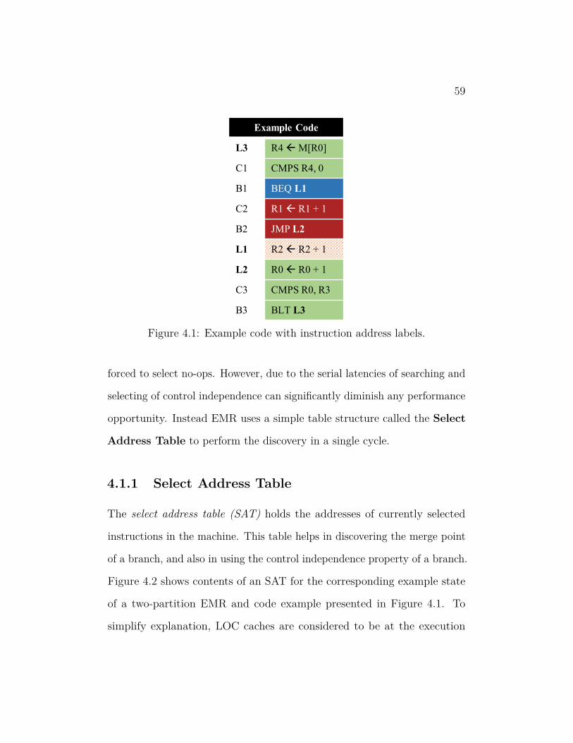
59
Example Code
L3 R4 M[R0]
C1 CMPS R4, 0
B1 BEQ L1
C2 R1 R1 + 1
B2 JMP L2
L1 R2 R2 + 1
L2 R0 R0 + 1
C3 CMPS R0, R3
B3 BLT L3
Figure 4.1: Example code with instruction address labels.
forced to select no-ops. However, due to the serial latencies of searching and
selecting of control independence can significantly diminish any performance
opportunity. Instead EMR uses a simple table structure called the Select
Address Table to perform the discovery in a single cycle.
4.1.1 Select Address Table
The select address table (SAT) holds the addresses of currently selected
instructions in the machine. This table helps in discovering the merge point
of a branch, and also in using the control independence property of a branch.
Figure 4.2 shows contents of an SAT for the corresponding example state
of a two-partition EMR and code example presented in Figure 4.1. To
simplify explanation, LOC caches are considered to be at the execution

60
LATCH
LATCH
R4 M[R0]
CMPS R4, 0
BEQ L1
R1 R1 + 1
JMP L2
R0 R0 + 1
CMPS R0, R3
BLT L3
SAT
L3
C1
B1
C2
B2
L2
C3
B3
LATCH
LATCH
R4 M[R0]
CMPS R4, 0
BEQ L1
R0 R0 + 1
CMPS R0, R3
BLT L3
SAT
L3
C1
B1
L1
L2
C3
B3
R2 R2 + 1
Figure 4.2: Examples of contents of select address table when two differentpaths of a branch are selected.
station granularity rather than the proposed partition granularity. The two
parts of the example show different SAT states when the branch selects one
path or the other.
SAT is mainly used to detect the first control independent instruction,
and hence the merge point of a control flow divergence. The aggressiveness
of control independence detection can also be controlled by the way SAT is
populated.

61
4.1.2 Merge Point Detection
Discovery of CI instruction is enabled after a mispredicted branch resolves.
Each partition younger than the mispredicted branch, will look up the SAT
and its LOC$ with the incoming address. When SAT is looked up with an
address, an associative search is done to find the oldest younger partition
that has selected this instruction bundle. If SAT look up results in a match,
the current partition selects no-ops and propagates input values to outputs.
In case SAT look up did not yield a match, LOC$ might supply the required
instruction bundle using In-place fetch. Thresholding the distance of CI
instruction can be done to limit the no-op partitions.
Consider the example illustrated in the Figure 4.2. When the branch
BEQ L1 resolves as a taken branch, instead of the predicted not-taken
branch, control independence discovery is enabled. When execution station
3 of the first partition receives the address L1, the SAT is looked up for this
address in parallel to the LOC$ look up. Since the instruction corresponding
to the target address (L1) is currently not selected at any of the entries
in the machine, the LOC$ of execution station 3 would have provided this
instruction. Following an LOC$ miss at the execution station 3 of the first
partition, the same look up procedure is repeated at execution station 0 of
the second partition. Since the instruction corresponding to the address L1
is present in the LOC$ of the execution station 0 of the second partition, it
is selected and the next address corresponding to the control independent
instruction R0<—R0+1 is generated. As execution station 1 of the second

62
partition looks up the SAT, it finds that this instruction is actually being
selected by an entry in the close proximity — in this case the same execution
station. This marks the end of control independence discovery and since the
incoming addresses did not change, existing selected instructions retain their
execution state and results. In CRIB, instructions are re-executed when the
source value changes. These changes in source values are detected by the
toggling of ready bits associated with the source registers. This is done so
that a mispredicted load instruction, instead of causing a pipeline squash,
requires only its dependent instructions to replay. The same technique is used
to take care of reevaluating any control independent data dependent(CIDD)
instructions.
4.2 Trade Offs in Control Independence
Control independence trade offs have been studied earlier by Agarwal et al.
where critical instruction fetch can be delayed due to utilization of control
independence [1]. Additionally, the effects of control independence on branch
predictors was presented by Michael and Koppelman [71]. In EMR, the
detrimental effect of pursuing control independence is the decreased effective
instruction window size.
The aggressiveness of CI instruction discovery can be controlled by
thresholding the distance of CI instruction’s partition from the current
partition, and by the way the SAT is populated. The distance of a control

63
independent instruction’s partition from the current partition that is search-
ing for the control independent instruction is obtained as the measure of
number of intermediate partitions that have to select no-ops in order to
propagate the precise architectural state to the control independent parti-
tion. Thresholding this distance can limit the discovery range of a control
independent instruction. The SAT can be populated either aggressively
or conservatively. An aggressive way is to update the SAT entry when
instruction bundle is selected by the corresponding partition. Alternatively,
a more conservative approach would be to update the SAT entry when at
least one of the instructions in the corresponding partition starts to execute.
While aggressive CI instruction discovery results in more opportunities,
they tend to hurt performance in many benchmarks. As intermediate
partitions select no-ops, they decrease the effective window size and limit
instruction level parallelism. Additionally, since completed CIDI instructions
are the main benefactors to performance, the conservative approach is
observed to be a better choice. A trade off analysis also showed that limiting
threshold distance, used to find the CI instruction, results in best overall
performance. This analysis is presented in Section 6.3.4 of Chapter 6.
4.3 Case Study of Astar
A-star, or 473.astar, is a SPEC2006 benchmark that is derived from a
portable two-dimensional path-finding library that is used in artificial in-
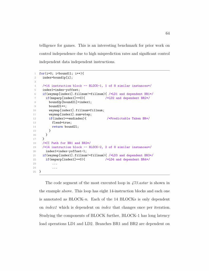
64
telligence for games. This is an interesting benchmark for prior work on
control independence due to high misprediction rates and significant control
independent data independent instructions.
1 for(i=0; i<bound1l; i++){2 index=bound1p[i];34 /*14 instruction block -- BLOCK-1, 1 of 8 similar instances*/5 index1=index-yoffset;6 if(waymap[index1].fillnum!=fillnum){ /*LD1 and dependent BR1*/7 if(maparp[index1]==0){ /*LD2 and dependent BR2*/8 bound2p[bound2l]=index1;9 bound2l++;
10 waymap[index1].fillnum=fillnum;11 waymap[index1].num=step;12 if(index1==endindex){ /*Predictable Taken BR*/13 flend=true;14 return bound2l;15 }16 }17 }18 /*CI Path for BR1 and BR2*/19 /*14 instruction block -- BLOCK-2, 2 of 8 similar instances*/20 index1=index-yoffset-1;21 if(waymap[index1].fillnum!=fillnum){ /*LD3 and dependent BR3*/22 if(maparp[index1]==0){ /*LD4 and dependent BR4*/23 ...24 ...25 }
The code segment of the most executed loop in 473.astar is shown in
the example above. This loop has eight 14-instruction blocks and each one
is annotated as BLOCK-n. Each of the 14 BLOCKs is only dependent
on index1 which is dependent on index that changes once per iteration.
Studying the components of BLOCK further, BLOCK-1 has long latency
load operations LD1 and LD2. Branches BR1 and BR2 are dependent on
65
these load operations and are hard to predict. With presence of significant
ILP across different BLOCKs, there are considerable long-latency control
independent data independent instructions for both BR1 and BR2 within
an acceptable distance. When BR1 or BR2 mispredict, the completed CIDI
instructions, LD3 and LD4 and their dependents, are used to further enhance
EMR performance.
4.4 Summary
A novel way to discover and utilize control independence was presented as
an extension to EMR. A select address table is used to precisely discover the
control independent instructions, if they exist in the machine. A through
evaluation is presented in Chapter 6.

66
5 amplified instruction
deliveryFlynn’s bottleneck is an observation that the instructions committed per
clock (IPC) can not exceed the instructions fetched per clock [117]. Although
a nuance, a more accurate statement, to encompass µop caches, loop buffers
or other such instruction storage, would be to say that IPC can not exceed
the instructions supplied for processing in a clock cycle.
The in-place-fetch mechanism in EMR enables optimizations to increase
the number of instructions that are delivered for execution without changing
the front-end bandwidth. In this chapter, the technique to amplify instruc-
tion delivery bandwidth to the execution cores is explained. Henceforth,
this thesis refers to this technique as AID. Like the loop buffers or µop
caches, this technique can also improve the transient fetch bandwidth of the
machine and can increase the Flynn’s bottleneck limit on performance.
5.1 Relaxing the Flynn’s Bottleneck Limit
EMR uses a novel speculative technique to supply instructions from the
partition-local caches to increase the number of instructions that can be,
in conventional terms, fetched in a single cycle. AID is supplemented by
increased commit bandwidth to boost performance. In this section, the
67
necessary modifications to increase commit bandwidth is discussed first,
followed by a detailed explanation of the amplified instruction delivery
technique.
5.1.1 Increased Commit Width
Committing more than one partition in a cycle requires simple, yet non-trivial
change in the baseline CRIB. While it is simple, due to Flynn’s bottleneck,
committing more than one partition per cycle boosts performance only
if more than one partition can be allocated in a cycle. If the front-end
bandwidth does not change, CRIB does not need to commit more than one
partition at a time.
Since EMR is a derivative of CRIB, the changes required to commit
more than one partition still remains straight forward. Although multiple
partitions can be committed per cycle, this work limits the number of
committed partitions to two. All the explanations relating to AID will be
explained assuming that two partitions are committed in a cycle. Once two
partitions are committed, AID can supply instructions to both partitions
in a single cycle. Assuming that each partition can hold four instructions,
AID can increase the theoretical limit of IPC from four to eight.
With increased commit width, when a partition is ready to commit, the
commit logic checks if more than one partition is ready to commit. If both
partitions are ready, a check for presence of instruction execution faults
has to be handled. In absence of any instruction faults, both partitions

68
are committed and the partition following the second of the committed
partitions is made as the architected partition.
5.1.2 Amplified Instruction Delivery
When a partition commits, the incoming address from the previous partition,
which is no longer blocked, will be used to select an appropriate instruction
bundle. In steady state, the committed partition is likely to select a new
instruction bundle and generate the instruction address for the following
partition. The partition following the committed partition will become the
architected partition signifying that the partition is executing the oldest
instruction bundle in the instruction window. If the newly promoted archi-
tected partition does not commit in a cycle, it can receive the address of
the instruction bundle that it has to select after commit.
Assume a two-partition i.e., eight instruction commit in EMR with
front end delivering four instructions per cycle. When two partitions are
committed in a cycle, the first partition immediately selects an instruction
bundle from LOC$ based on incoming address and delivers the first set of four
instructions. Since the second partition would get a valid incoming address
only after a cycle, in-place fetch would deliver only four instructions per
clock. So, Flynn’s bottleneck would still limit the theoretical performance
to four instructions per cycle.
An observation can be made that once a partition is promoted to be the
architected partition, the incoming address will no longer change. So the

69
partition control unit can be used to generate the instruction address for
the partition following the architected partition. Now, when two partitions
commit in a cycle, the second partition would have a valid instruction
address to select from. This way, two instruction bundles or up to eight
instructions can be selected in a single clock cycle after committing two
partitions. This technique fails if EMR consistently commits more than one
partition in a cycle.
5.1.3 Next-Index Prediction
Next-index prediction is used as a simple alternative to provide an instruction
bundle to the second of the two partitions that committed in a cycle, given
that pre-computation was not possible. The second partition uses a simple
next-index predictor to speculatively select an instruction bundle in the
same cycle as the first partition. The next-index predictor, local to each
partition, is a simple table that is accessed by using the current index of
the LOC$ and the entry provides the next-index of the LOC$. Instead of
an associative lookup, LOC$ data array is directly looked up using this
index value to obtain the instruction bundle. The prediction is verified and
corrected, if necessary, in the next cycle as the partition gets the actual
address. With invalid initial values, this predictor is updated every time the
associated partition selects based on incoming address.
As an example, consider the entries of this next-index predictor as shown
in Table 5.1, assuming eight entries per LOC$. The first four indices show

70
Current Index Next Index0 11 22 33 04 -5 46 47 7
Table 5.1: Example contents of Next-index predictor which is used to amplifyinstruction delivery.
a pattern of a long loop that is captured across multiple partitions across
multiple LOC$ entries. An entry, like the one at index four, can have an
invalid value to avoid predicting incorrectly. Entries at indices five and six
show a pattern of backward branches that can correspond to continue like
statements. There can be entries that have the same value as the select
index, implying that the loops are properly captured within the execution
window.
The performance impact of AID is dependent on factors other than the
accuracy of the next-index predictor. Program and machine characteristics
determine the scenarios where two partitions commit in a single cycle. Even
if such opportunities are frequent, long latency instructions and branch
mispredictions can limit the performance gains from AID. The performance
analysis of AID, double commit opportunity and the accuracy of next-index
predictor are presented in Section 6.2.3 in Chapter 6.
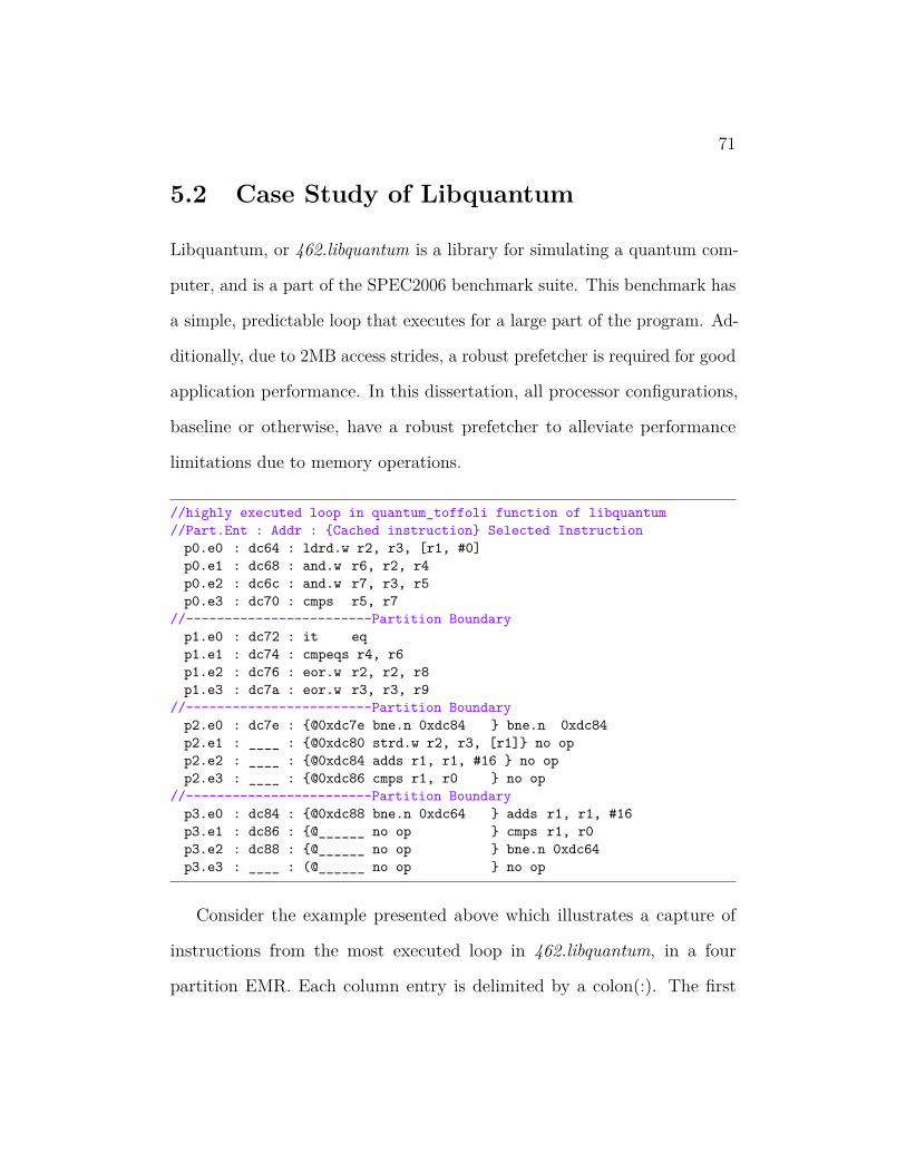
71
5.2 Case Study of Libquantum
Libquantum, or 462.libquantum is a library for simulating a quantum com-
puter, and is a part of the SPEC2006 benchmark suite. This benchmark has
a simple, predictable loop that executes for a large part of the program. Ad-
ditionally, due to 2MB access strides, a robust prefetcher is required for good
application performance. In this dissertation, all processor configurations,
baseline or otherwise, have a robust prefetcher to alleviate performance
limitations due to memory operations.
//highly executed loop in quantum_toffoli function of libquantum//Part.Ent : Addr : {Cached instruction} Selected Instruction
p0.e0 : dc64 : ldrd.w r2, r3, [r1, #0]p0.e1 : dc68 : and.w r6, r2, r4p0.e2 : dc6c : and.w r7, r3, r5p0.e3 : dc70 : cmps r5, r7
//------------------------Partition Boundaryp1.e0 : dc72 : it eqp1.e1 : dc74 : cmpeqs r4, r6p1.e2 : dc76 : eor.w r2, r2, r8p1.e3 : dc7a : eor.w r3, r3, r9
//------------------------Partition Boundaryp2.e0 : dc7e : {@0xdc7e bne.n 0xdc84 } bne.n 0xdc84p2.e1 : ____ : {@0xdc80 strd.w r2, r3, [r1]} no opp2.e2 : ____ : {@0xdc84 adds r1, r1, #16 } no opp2.e3 : ____ : {@0xdc86 cmps r1, r0 } no op
//------------------------Partition Boundaryp3.e0 : dc84 : {@0xdc88 bne.n 0xdc64 } adds r1, r1, #16p3.e1 : dc86 : {@______ no op } cmps r1, r0p3.e2 : dc88 : {@______ no op } bne.n 0xdc64p3.e3 : ____ : (@______ no op } no op
Consider the example presented above which illustrates a capture of
instructions from the most executed loop in 462.libquantum, in a four
partition EMR. Each column entry is delimited by a colon(:). The first
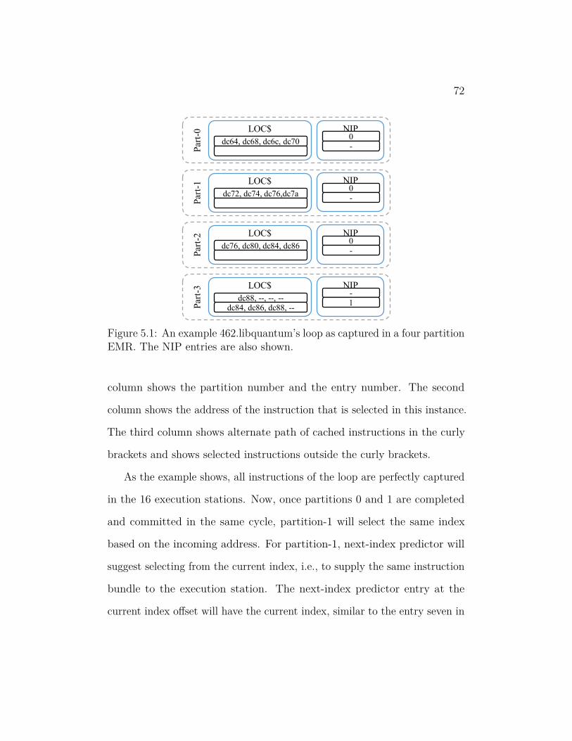
72
dc64, dc68, dc6c, dc70
Par
t-0 LOC$
dc72, dc74, dc76,dc7aP
art-
1 LOC$
dc76, dc80, dc84, dc86
Par
t-2 LOC$
dc88, --, --, --dc84, dc86, dc88, --P
art-
3 LOC$
NIP0-
NIP0-
NIP0-
NIP-1
Figure 5.1: An example 462.libquantum’s loop as captured in a four partitionEMR. The NIP entries are also shown.
column shows the partition number and the entry number. The second
column shows the address of the instruction that is selected in this instance.
The third column shows alternate path of cached instructions in the curly
brackets and shows selected instructions outside the curly brackets.
As the example shows, all instructions of the loop are perfectly captured
in the 16 execution stations. Now, once partitions 0 and 1 are completed
and committed in the same cycle, partition-1 will select the same index
based on the incoming address. For partition-1, next-index predictor will
suggest selecting from the current index, i.e., to supply the same instruction
bundle to the execution station. The next-index predictor entry at the
current index offset will have the current index, similar to the entry seven in

73
example presented in Table 5.1. Figure 5.1 shows a sample capture of the
loop in a four partition EMR with two LOC$ entries. The figure also shows
an example state of next-index predictor, which is correct most of the times.
As the loops are tightly packed, there is significant opportunity available in
462.libquantum, resulting in sizeable performance gains from AID.
5.3 Summary
This chapter presented a novel extension idea to EMR, AID, to increase
the number of instructions delivered to the back end without increasing the
front end bandwidth. AID uses a combination of pre-computation of next
address and next-index predictor to help relax the performance limit placed
by Flynn’s bottleneck in the baseline processors.

74
6 evaluationEMR has been thoroughly evaluated with a wide variety of benchmarks
using a cycle accurate simulator and energy estimation tool. Using these
tools, various characteristics of EMR, and various design trade offs have
been documented in this chapter. This chapter starts with the details on
the evaluation platform followed by presenting actual experiments and their
results.
In these evaluations, it is observed that EMR outperforms CRIB by
23%, 20%, 10.5% and 4% in CINT2006, MiBench, Graph500 and CFP2006
respectively. Additionally, on an average, EMR saves 16%, 17%, 13% and
25% of the baseline energy when running CINT2006, MiBench, Graph500
and CFP2006 respectively.
6.1 Evaluation Setup
The evaluation platform consists of a cycle accurate simulator, an energy
estimation tool, configurations of baseline and EMR machines and bench-
marks.
6.1.1 Cycle Accurate Simulator
A new cycle-accurate, execute-at-execute CRIB CPU model is implemented
in gem5 [7] and is thoroughly validated using SPEC 2006 [38], MiBench [31],

75
SDVBS [123] and Graph500 [75] benchmarks. Execute-at-execute enforces
tighter implementation requirements for functional correctness and provides
realistic scenarios when predictions are involved. Numerous parametric
studies with sanity, statistical and manual verifications boost confidence in
the accuracy of the implemented CRIB model. Some inconsistencies in the
O3 model of gem5, like the presence of unnecessary "bubbles" in the pipeline
are fixed to make a fair comparison in Figure 2.6. The LTAGE branch
predictor is implemented and verified against the LTAGE from the branch
predictor championships. Ideal branch prediction is achieved by dumping
the trace of actual outcomes and using them as predictions in a subsequent
run of the benchmark.
6.1.2 Machine Configurations
Table 6.1 shows configurations of different machines considered in this paper.
In various experiments, the execution window size, LOC$ and ICU$ sizes
are modified to observe the performance impact of these variables.
In CRIB, the instruction window size is determined by the number
of execution stations. The baseline conventional out-of-order processor is
modeled using the architectural parameters from Intel’s Haswell microarchi-
tecture [34]. To match the performance of this processor, the baseline CRIB
is configured to have 64 execution stations.
The issue queue entries in conventional out-of-order is assumed to be
a unified issue queue and is modelled using the state-of-the-art processors
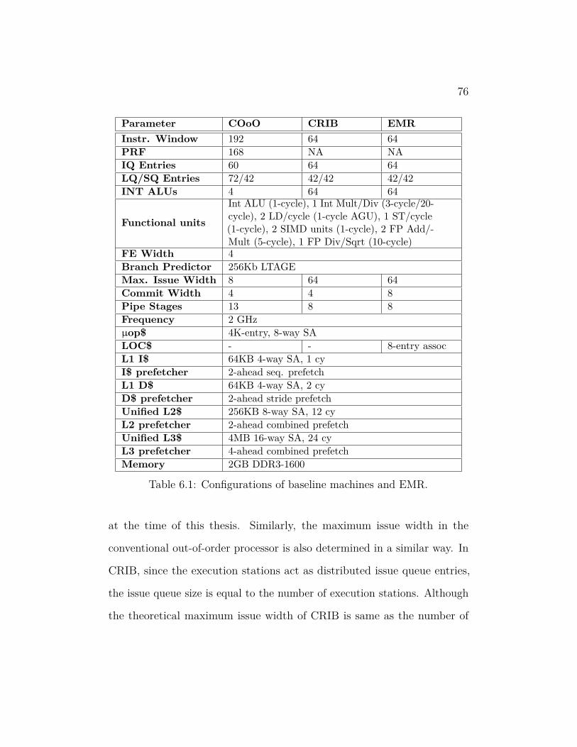
76
Parameter COoO CRIB EMRInstr. Window 192 64 64PRF 168 NA NAIQ Entries 60 64 64LQ/SQ Entries 72/42 42/42 42/42INT ALUs 4 64 64
Functional units
Int ALU (1-cycle), 1 Int Mult/Div (3-cycle/20-cycle), 2 LD/cycle (1-cycle AGU), 1 ST/cycle(1-cycle), 2 SIMD units (1-cycle), 2 FP Add/-Mult (5-cycle), 1 FP Div/Sqrt (10-cycle)
FE Width 4Branch Predictor 256Kb LTAGEMax. Issue Width 8 64 64Commit Width 4 4 8Pipe Stages 13 8 8Frequency 2 GHzµop$ 4K-entry, 8-way SALOC$ - - 8-entry assocL1 I$ 64KB 4-way SA, 1 cyI$ prefetcher 2-ahead seq. prefetchL1 D$ 64KB 4-way SA, 2 cyD$ prefetcher 2-ahead stride prefetchUnified L2$ 256KB 8-way SA, 12 cyL2 prefetcher 2-ahead combined prefetchUnified L3$ 4MB 16-way SA, 24 cyL3 prefetcher 4-ahead combined prefetchMemory 2GB DDR3-1600
Table 6.1: Configurations of baseline machines and EMR.
at the time of this thesis. Similarly, the maximum issue width in the
conventional out-of-order processor is also determined in a similar way. In
CRIB, since the execution stations act as distributed issue queue entries,
the issue queue size is equal to the number of execution stations. Although
the theoretical maximum issue width of CRIB is same as the number of

77
execution station entries, it is unlikely that all the instructions in a window
are ready to execute at the same time. The typical issue width of CRIB is
much lower than the theoretical maximum but higher than the typical issue
widths of the conventional out-of-order baseline.
In CRIB, load or store queue entries can be allocated after the address
of a load or a store are available. This reduces the required number of load
and store queue entries in CRIB. Additionally, load and store queues can be
banked based on the memory address resulting in reduced area, power and
access delays for these structures. Due to the consolidation of rename, issue
queue, bypass, ALUs, and reorder buffer into a single stage, the number of
pipelines in baseline CRIB are much lower than the baseline conventional
out-of-order processor.
Compared to CRIB presented in [30], the baseline CRIB modelled here
uses larger instruction window, larger number of load store queue entries
and unified integer and floating point CRIB. Additionally, the component
delays have been recalibrated to increase the propagation from four to eight.
The load queue and store queue sizes are appropriately sized for the 64 entry
instruction window and are two-way banked instead of four-way banked
assumption in Erika’s evaluation [30]. The Table 6.1 shows the cumulative
number of load and store queue entries for CRIB and EMR.

78
6.1.3 Energy Model
The power model of McPat [62] is modified to correlate to the CRIB power
numbers as presented in [30]. The energy savings due to µop cache are
also incorporated into McPat model to provide the power estimates of the
baseline CRIB processor. The µop$ is accessed in every active fetch cycle
and is written when the instruction bundle is not found in the µop cache.
The main energy savings in µop$ comes by reducing partial I$ energy and
full energies of variable length decode and decode units.
For the LOC$ access energy, the access energy obtained from Fabmem [16]
is correlated with the Cacti [74] model used in McPat. The LOC$ access
energy is doubled as a conservative estimate of additional component power
and incorporated these metrics into the McPat model. In addition, leakage
power of the LOC and ICU caches are considered for energy calculation. All
FE provided instructions, in addition to the FE energy, also consume energy
for writes into ICU$ and LOC$. However, when the FE is turned off, all of
I$, variable length decode and Decode energies are saved. Instead of looking
up on every fetch cycle, ICU$ is looked up only when LOC$ misses. When
ICU$ supplies an instruction to LOC$, in addition to the ICU$ read energy,
LOC$ write energy is also consumed. Irrespective of hit or miss, each LOC$
lookup consumes read energy. The power estimates from McPat and the
execution time of each program are used to generate energy estimates. It can
be observed from these static components that availability of instructions in
LOC$ will have a significant impact on energy consumption in EMR.
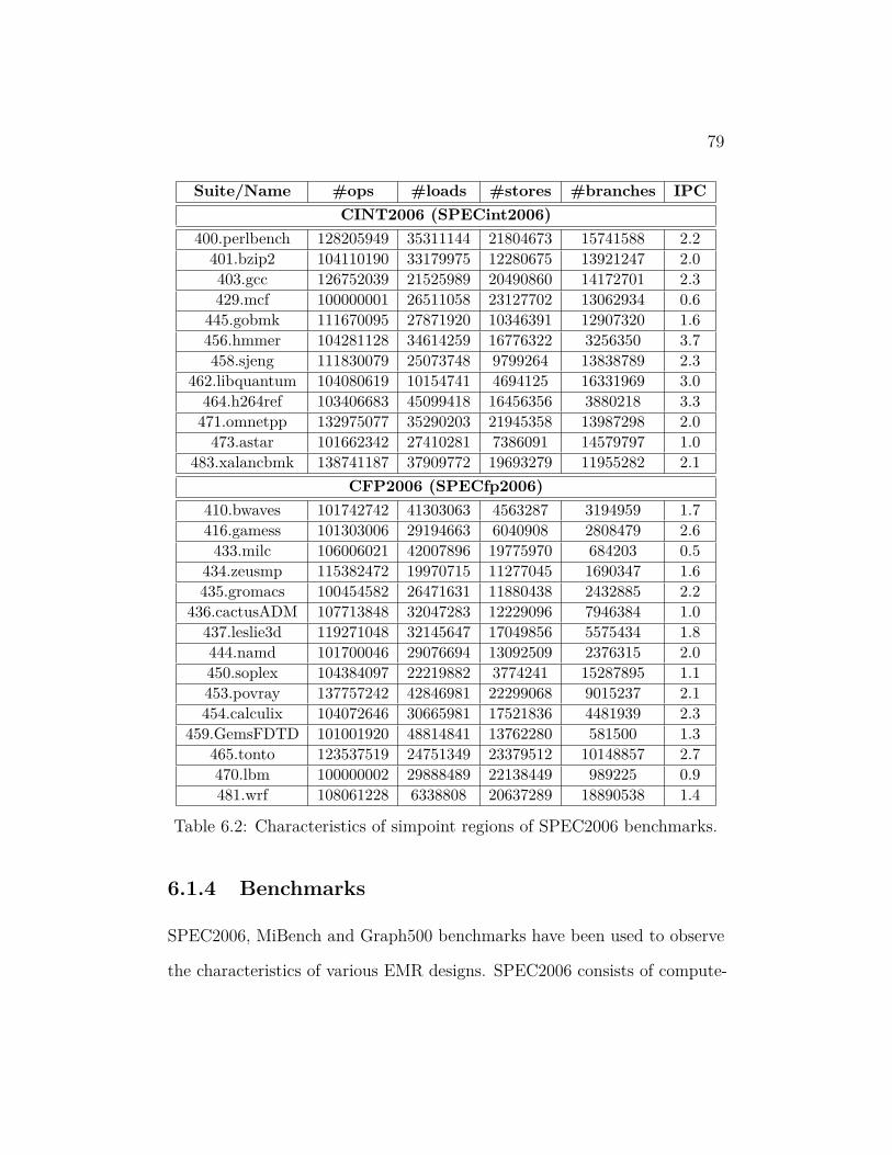
79
Suite/Name #ops #loads #stores #branches IPCCINT2006 (SPECint2006)
400.perlbench 128205949 35311144 21804673 15741588 2.2401.bzip2 104110190 33179975 12280675 13921247 2.0403.gcc 126752039 21525989 20490860 14172701 2.3429.mcf 100000001 26511058 23127702 13062934 0.6
445.gobmk 111670095 27871920 10346391 12907320 1.6456.hmmer 104281128 34614259 16776322 3256350 3.7458.sjeng 111830079 25073748 9799264 13838789 2.3
462.libquantum 104080619 10154741 4694125 16331969 3.0464.h264ref 103406683 45099418 16456356 3880218 3.3471.omnetpp 132975077 35290203 21945358 13987298 2.0
473.astar 101662342 27410281 7386091 14579797 1.0483.xalancbmk 138741187 37909772 19693279 11955282 2.1
CFP2006 (SPECfp2006)410.bwaves 101742742 41303063 4563287 3194959 1.7416.gamess 101303006 29194663 6040908 2808479 2.6433.milc 106006021 42007896 19775970 684203 0.5
434.zeusmp 115382472 19970715 11277045 1690347 1.6435.gromacs 100454582 26471631 11880438 2432885 2.2
436.cactusADM 107713848 32047283 12229096 7946384 1.0437.leslie3d 119271048 32145647 17049856 5575434 1.8444.namd 101700046 29076694 13092509 2376315 2.0450.soplex 104384097 22219882 3774241 15287895 1.1453.povray 137757242 42846981 22299068 9015237 2.1454.calculix 104072646 30665981 17521836 4481939 2.3
459.GemsFDTD 101001920 48814841 13762280 581500 1.3465.tonto 123537519 24751349 23379512 10148857 2.7470.lbm 100000002 29888489 22138449 989225 0.9481.wrf 108061228 6338808 20637289 18890538 1.4
Table 6.2: Characteristics of simpoint regions of SPEC2006 benchmarks.
6.1.4 Benchmarks
SPEC2006, MiBench and Graph500 benchmarks have been used to observe
the characteristics of various EMR designs. SPEC2006 consists of compute-

80
Suite/Name #ops #loads #stores # br IPCMiBench
auto.bitcnt 50560084 2480863 603897 4629619 2.5auto.qsort 71986654 13509620 10318829 9898641 2.1auto.susan.corners 22182996 8419240 2363952 1065980 2.8auto.susan.edges 64474732 25702689 8391782 2871161 2.9auto.susan.smoothing 263040999 76172718 502928 27005516 2.5cons.cjpeg 104434305 28750469 15563063 10196961 2.9cons.djpeg 23433699 6949167 3447864 1221973 3.4cons.lame 1129184352 331114418 133009996 70304970 1.9cons.mad 294506143 105603280 42671651 11333355 2.7cons.tiff2bw 147256337 39663390 19258287 10940661 3.9cons.tiff2rgba 386852520 116697880 56504695 63221593 2.5cons.tiffdither 606240672 68635779 54483073 35117089 3.0cons.tiffmedian 613275741 149526153 95415416 24917042 3.4net.dijkstra 190278062 37600689 19194753 42801675 1.8net.patricia 749955544 134358190 91376348 81983497 2.7off.rsynth 544214956 199957636 75818846 38322153 1.6off.stringsearch 5582534 727926 776150 1006129 3.0sec.blowfish 299822680 71262678 27229038 20100983 2.4sec.rijndael 457089776 138675069 70459927 16057901 3.4sec. sha 116469923 16464187 9049205 5646925 3.7tele.adpcm.compress 719189229 53355825 6692975 66629877 2.5tele.adpcm.decompress 519562195 33410731 13345775 46656613 3.5tele.crc 234766152 61162535 6958882 27693685 1.3tele.fft 14740146 1641187 1050285 868903 2.6tele.gsm 1171687816 366425136 149423693 67613735 2.0
Graph500seq-csr 441146604 34375030 26064063 20909240 2.7seq-list 440364969 33946970 24117953 24027246 2.1
Table 6.3: Characteristics of MiBench and Graph500.
intensive programs developed from real user applications, and are used
widely in evaluating various processor designs. For SPEC 2006 benchmarks,
Simpoint [100] analysis is done to determine the best performance correlating
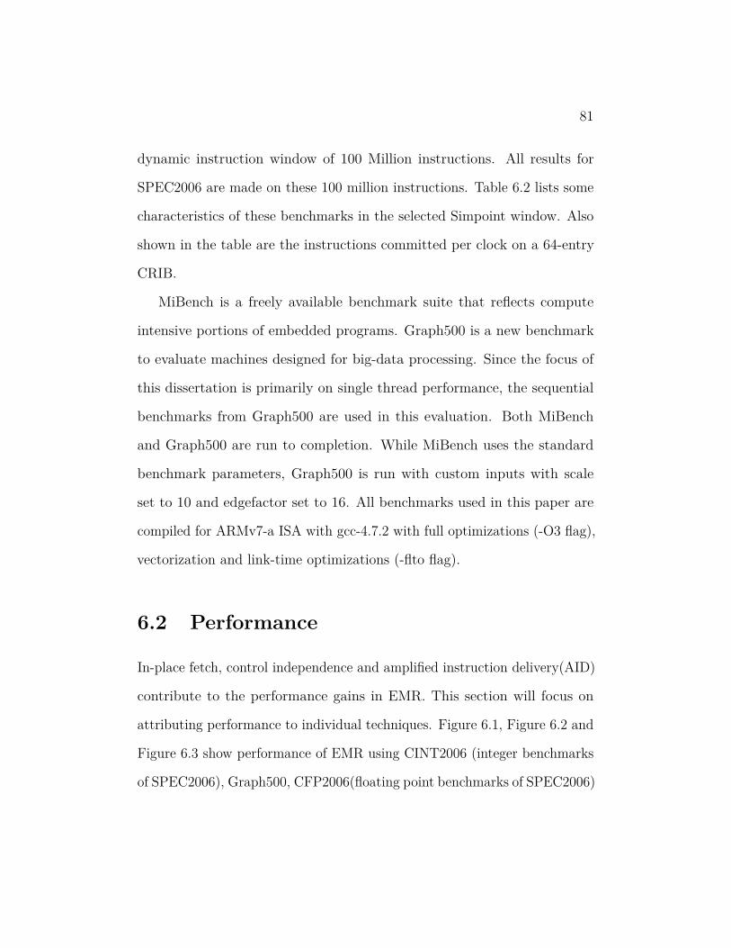
81
dynamic instruction window of 100 Million instructions. All results for
SPEC2006 are made on these 100 million instructions. Table 6.2 lists some
characteristics of these benchmarks in the selected Simpoint window. Also
shown in the table are the instructions committed per clock on a 64-entry
CRIB.
MiBench is a freely available benchmark suite that reflects compute
intensive portions of embedded programs. Graph500 is a new benchmark
to evaluate machines designed for big-data processing. Since the focus of
this dissertation is primarily on single thread performance, the sequential
benchmarks from Graph500 are used in this evaluation. Both MiBench
and Graph500 are run to completion. While MiBench uses the standard
benchmark parameters, Graph500 is run with custom inputs with scale
set to 10 and edgefactor set to 16. All benchmarks used in this paper are
compiled for ARMv7-a ISA with gcc-4.7.2 with full optimizations (-O3 flag),
vectorization and link-time optimizations (-flto flag).
6.2 Performance
In-place fetch, control independence and amplified instruction delivery(AID)
contribute to the performance gains in EMR. This section will focus on
attributing performance to individual techniques. Figure 6.1, Figure 6.2 and
Figure 6.3 show performance of EMR using CINT2006 (integer benchmarks
of SPEC2006), Graph500, CFP2006(floating point benchmarks of SPEC2006)
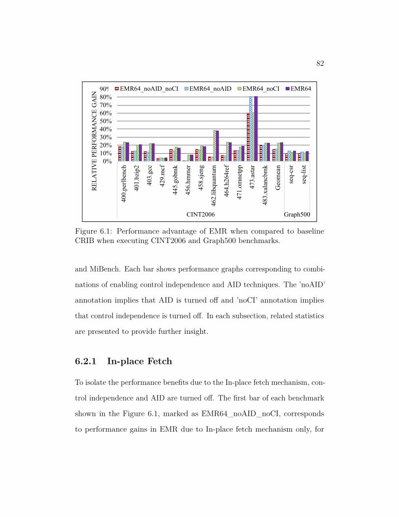
82
0%
10%
20%
30%
40%
50%
60%
70%
80%
90%
40
0.p
erlb
ench
40
1.b
zip2
40
3.g
cc
429.m
cf
44
5.g
obm
k
45
6.h
mm
er
458.s
jeng
462
.lib
qu
antu
m
46
4.h
264re
f
471
.om
net
pp
473
.ast
ar
483
.xal
ancb
mk
Geo
mea
n
seq
-csr
seq-l
ist
CINT2006 Graph500
RE
LA
TIV
E P
ER
FO
RM
AN
CE
GA
INEMR64_noAID_noCI EMR64_noAID EMR64_noCI EMR64
Figure 6.1: Performance advantage of EMR when compared to baselineCRIB when executing CINT2006 and Graph500 benchmarks.
and MiBench. Each bar shows performance graphs corresponding to combi-
nations of enabling control independence and AID techniques. The ’noAID’
annotation implies that AID is turned off and ’noCI’ annotation implies
that control independence is turned off. In each subsection, related statistics
are presented to provide further insight.
6.2.1 In-place Fetch
To isolate the performance benefits due to the In-place fetch mechanism, con-
trol independence and AID are turned off. The first bar of each benchmark
shown in the Figure 6.1, marked as EMR64_noAID_noCI, corresponds
to performance gains in EMR due to In-place fetch mechanism only, for

83
CINT2006 and Graph500. These performance gains are largely attributed to
reduced execution-resume delay. Other benefits from In-place fetch include
reduced pipeline stalls and front end squashes. These front end stalls can be
caused due to I$ access stalls. Branch check at the decode stage can squash
the front end to correct mispredicted targets of direct branches.
Benchmarks with significant branch mispredictions benefit a lot from
the reduced the ER delay. 471.astar leads the performance curve with a
massive 60% performance gain with a geometric mean performance gain of
14% in CINT2006 and 9.5% in Graph500. Most of the benchmarks have
this performance gain correlated to the branch predictor MPKI, as shown in
Figure 1.2. 429.mcf, due to high cache miss rate, has a low 4% benefit even
with significant branch predictor MPKI of 9.2. In contrast, 462.libquantum
and 464.h264ref have small performance gains even without any significant
branch predictor MPKI. This is because EMR, even without AID, can
remove many pipeline bubbles when delivering instructions from back end
caches.
The In-place fetch benefits in CFP2006 are shown in the first bar of the
Figure 6.2. The moderate to trivial performance gains are due to the fact that
most programs in the CFP2006 have much lesser opportunity, as observed
from Figure 1.3. In cases like 436.cactusADM, where sizeable opportunity
exists, high-latency floating point operations and long dependence chains
limit performance. Like 462.libquantum, 437.leslie3d and 465.tonto have
small performance gains as a result of reduced pipeline bubbles in the

84
0%
2%
4%
6%
8%
10%
12%
410
.bw
aves
41
6.g
ames
s
43
3.m
ilc
434.z
eusm
p
43
5.g
rom
acs
43
6.c
actu
sAD
M
437
.les
lie3
d
44
4.n
amd
450.s
ople
x
45
3.p
ovra
y
45
4.c
alcu
lix
45
9.G
emsF
DT
D
465
.ton
to
470.l
bm
481.w
rf
Geo
mea
n
RE
LA
TIV
E P
ER
FO
RM
AN
CE
GA
INEMR_noCI_noAID EMR_noAID EMR_noCI EMR
Figure 6.2: Performance gains of EMR relative to the performance of baselineCRIB when executing CFP2006.
front end. Overall, EMR, with in-place fetch alone, provides a 2% mean
performance boost to CFP2006 applications.
The first bar of Figure 6.3 shows the speedups in MiBench when only In-
place fetch mechanism is used in EMR. In MiBench, qsort, in the automotive
category executes 44% faster on EMR over the baseline. As Figure 1.4
shows, the 17 branch predictor MPKI provides substantial opportunity to
gain performance in this benchmark. With the exception of tiffbw, all other
benchmarks in the consumer category gain substantially from in-place fetch
mechanism. patricia in the network category frequently misses the back end
caches, resulting in lower performance gain than what can be expected from
7.5 branch predictor MPKI. As a benchmark suite, MiBench runs 8% faster
85
0%
10%
20%
30%
40%
50%
60%
70%
bit
cnt
qso
rtsu
san.c
..su
san.e
..su
san.s
..cj
peg
djp
egla
me
mad
tiff
2b
wti
ff2rg
ba
tiff
dit
her
tiff
med
ian
dij
kst
rapat
rici
ars
ynth
stri
ng
s..
blo
wfi
shri
jndae
lsh
aad
pcm
.c..
adp
cm.d
..cr
cff
tgsm
Geo
mea
n
Automotive Consumer Net Offi Security Telecom O
RE
LA
TIV
E P
ER
FO
RM
AN
CE
GA
INEMR_noCI_noAID EMR_noAID EMR_noCI EMR
Figure 6.3: Relative performance of EMR when compared with baselineCRIB while evaluating MiBench.
on EMR than the CRIB baseline, when control independence and AID are
disabled.
6.2.2 Control Independence
The second bar in the Figure 6.1 shows the CINT2006 performance gains
when control independence is enabled in EMR. AID is still disabled for this
evaluation.
As observed from the figure, there are mixed performance trends. On
the upside, 471.astar gains an additional 21% performance, resulting in a
phenomenal 81% performance boost over the baseline. This performance
lines up with the expectation from the case study presented in Section 4.3

86
of Chapter 4. Graph500 benchmarks also gain marginally from enabling
control independence. On the flip side, some benchmarks, like 445.gobmk
loose about 2% performance when control independence is enabled. Such
losses are observed due to the trade offs discussed in Section 4.2 of Chapter 4.
As can be seen from the Figure 6.2 and Figure 6.3, control independence
does not help any of these benchmarks and hurts performance in some cases.
A point to note here is that control independence in EMR does not include
the benefits due to the reduced execution-resume time. Benefits, where
present, are mainly from eliminating re-execution of CIDI instructions.
6.2.3 Amplified Instruction Delivery
In the Figure 6.1, the third bar reports performance gains of EMR when
control independence is disabled and AID is enabled. As discussed in
Section 5.1.2 of Chapter 5, the performance expectation from AID can be
partially influenced by the number of times two partitions commit in a
cycle. The percentage of double partition commits reflects the opportunity
to amplify instruction delivery. Additionally, the accuracy of the next-index
predictor influences the ability to exploit the available opportunity. The first
bar in Figure 6.4 shows the percentage of double partition commits in each
program. The second bar in this figure shows the accuracy of the next-index
predictor(annotated as NIP in the graph). It is interesting to note that
the accuracy of the next-index predictor shows an inversely proportional
relationship with branch predictor MPKI of a benchmark.

87
0%10%20%30%40%50%60%70%80%90%
100%
400.p
erlb
ench
40
1.b
zip2
403.g
cc
42
9.m
cf
44
5.g
obm
k
456
.hm
mer
45
8.s
jeng
462.l
ibqu
antu
m
464.h
264re
f
471.o
mnet
pp
473.a
star
483.x
alan
cbm
k
Geo
mea
n
seq-c
sr
seq-l
ist
CINT2006 Graph500
OP
PO
RT
UN
ITY
/AC
CU
RA
CY
Double Partition Commit
NIP_Accuracy
Figure 6.4: Opportunity to amplify instruction delivery and the cumu-lative accuracy of the next-index predictors in CINT2006 and Graph500benchmarks.
While most benchmarks benefit from AID, 462.libquantum has a domi-
nant 38% performance gain. As can be seen from Figure 6.4, 462.libquantum
has both opportunity and high accuracy of the next-index predictor. The
underpinnings of this behavior is explained in Section 5.2 of Chapter 5.
429.mcf, 471.astar and seq-list have almost no benefits from AID due to a
combination of load misses and next-index prediction misses. EMR, when
using AID, boosts performance of CINT2006 by 22% over the baseline.
Although most benchmarks do not hit Flynn’s bottleneck limit when con-
sidered over the entire run of a program, transient bursts provide significant
boost in performance.
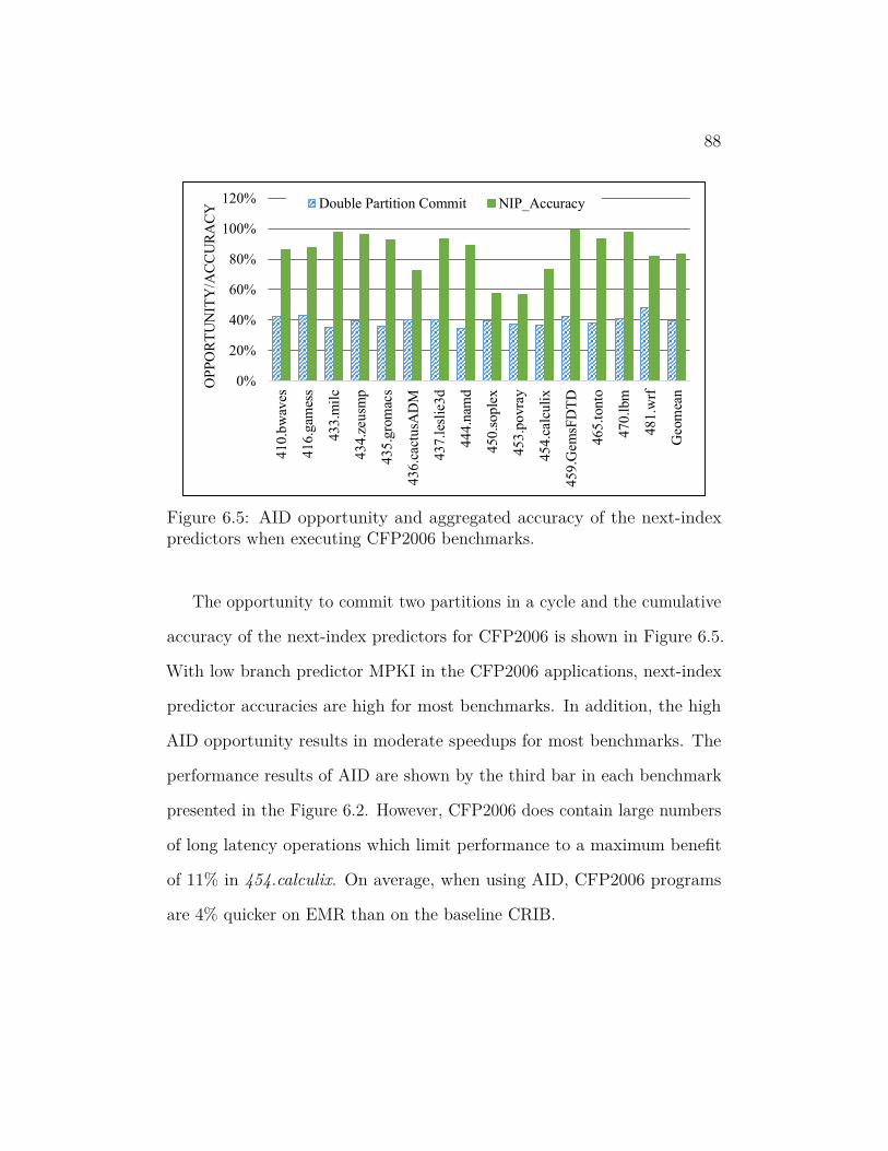
88
0%
20%
40%
60%
80%
100%
120%
410
.bw
aves
41
6.g
ames
s
43
3.m
ilc
434.z
eusm
p
43
5.g
rom
acs
43
6.c
actu
sAD
M
437
.les
lie3
d
44
4.n
amd
450.s
ople
x
45
3.p
ovra
y
454.c
alcu
lix
45
9.G
emsF
DT
D
46
5.t
on
to
47
0.l
bm
48
1.w
rf
Geo
mea
n
OP
PO
RT
UN
ITY
/AC
CU
RA
CY Double Partition Commit NIP_Accuracy
Figure 6.5: AID opportunity and aggregated accuracy of the next-indexpredictors when executing CFP2006 benchmarks.
The opportunity to commit two partitions in a cycle and the cumulative
accuracy of the next-index predictors for CFP2006 is shown in Figure 6.5.
With low branch predictor MPKI in the CFP2006 applications, next-index
predictor accuracies are high for most benchmarks. In addition, the high
AID opportunity results in moderate speedups for most benchmarks. The
performance results of AID are shown by the third bar in each benchmark
presented in the Figure 6.2. However, CFP2006 does contain large numbers
of long latency operations which limit performance to a maximum benefit
of 11% in 454.calculix. On average, when using AID, CFP2006 programs
are 4% quicker on EMR than on the baseline CRIB.
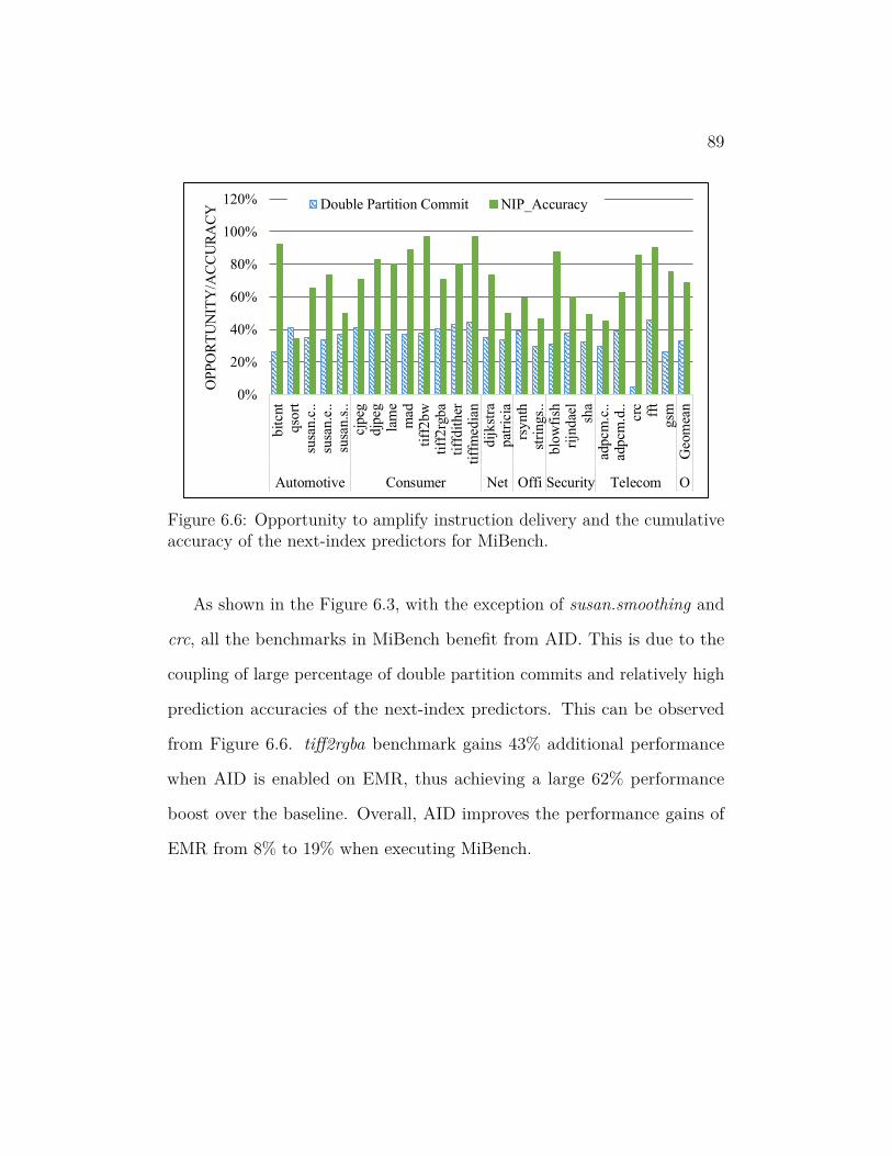
89
0%
20%
40%
60%
80%
100%
120%
bit
cnt
qso
rtsu
san.c
..su
san.e
..su
san.s
..cj
peg
djp
egla
me
mad
tiff
2b
wti
ff2rg
ba
tiff
dit
her
tiff
med
ian
dij
kst
rapat
rici
ars
ynth
stri
ng
s..
blo
wfi
shri
jndae
lsh
aad
pcm
.c..
adp
cm.d
..cr
cff
tgsm
Geo
mea
n
Automotive Consumer Net Offi Security Telecom O
OP
PO
RT
UN
ITY
/AC
CU
RA
CY Double Partition Commit NIP_Accuracy
Figure 6.6: Opportunity to amplify instruction delivery and the cumulativeaccuracy of the next-index predictors for MiBench.
As shown in the Figure 6.3, with the exception of susan.smoothing and
crc, all the benchmarks in MiBench benefit from AID. This is due to the
coupling of large percentage of double partition commits and relatively high
prediction accuracies of the next-index predictors. This can be observed
from Figure 6.6. tiff2rgba benchmark gains 43% additional performance
when AID is enabled on EMR, thus achieving a large 62% performance
boost over the baseline. Overall, AID improves the performance gains of
EMR from 8% to 19% when executing MiBench.
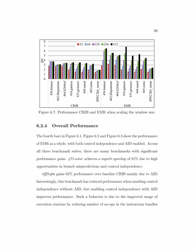
90
0
1
2
3
4
5
6
7
8
45
6.h
mm
er
462
.lib
qu
antu
m
46
4.h
264re
f
41
6.g
ames
s
435
.gro
mac
s
44
4.n
amd
465.t
onto
SP
EC
2k6_
mea
n
45
6.h
mm
er
462
.lib
qu
antu
m
46
4.h
264
ref
416
.gam
ess
435
.gro
mac
s
44
4.n
amd
465.t
onto
SP
EC
2k6_
mea
n
CRIB EMR
IPC
32 64 128 256 512
Figure 6.7: Performance CRIB and EMR when scaling the window size.
6.2.4 Overall Performance
The fourth bars in Figure 6.1, Figure 6.2 and Figure 6.3 show the performance
of EMR as a whole, with both control independence and AID enabled. Across
all three benchmark suites, there are many benchmarks with significant
performance gains. 473.astar achieves a superb speedup of 81% due to high
opportunities in branch mispredictions and control independence.
tiff2rgba gains 62% performance over baseline CRIB mainly due to AID.
Interestingly, this benchmark has reduced performance when enabling control
independence without AID, but enabling control independence with AID
improves performance. Such a behavior is due to the improved usage of
execution stations by reducing number of no-ops in the instruction bundles

91
0%
5%
10%
15%
20%
25%
30%
bit
cnt
qso
rt
susa
n.c
..
susa
n.e
..
susa
n.s
..
cjp
eg
djp
eg
lam
e
mad
tiff
2bw
tiff
2rg
ba
tiff
dit
her
tiff
med
ian
dij
kst
ra
pat
rici
a
rsy
nth
stri
ng
s..
blo
wfi
sh
rijn
dae
l
sha
adpcm
.c..
adpcm
.d..
crc
fft
gsm
Automotive Consumer Net Offi Security Telecom
NO
-OP
S /
PA
RT
ITIO
NEMR_noCI_noAID EMR_noAID EMR_noCI EMR
Figure 6.8: No-ops per partition in different configurations of EMR forMiBench.
when both AID and control independence are enabled and can be observed
from Figure 6.8.
Overall, when compared to the baseline, EMR has performance gain of
23% in CINT2006 and 12.5% in Graph500. Additional evaluations with
CFP2006 and MiBench show that EMR outperforms the baseline by 4%
and 20% respectively.
6.3 Performance Sensitivity Analysis
Various experiments were conducted to find the limitations and explore the
design space. In this section, a selected set of experiments and their results
on reduced set of benchmarks are presented.
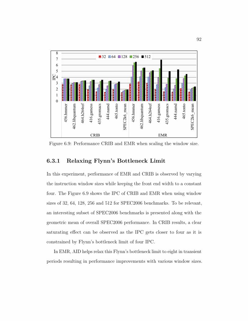
92
0
1
2
3
4
5
6
7
8
45
6.h
mm
er
462
.lib
qu
antu
m
46
4.h
264re
f
41
6.g
ames
s
435
.gro
mac
s
44
4.n
amd
465.t
onto
SP
EC
2k6_
mea
n
45
6.h
mm
er
462
.lib
qu
antu
m
46
4.h
264
ref
416
.gam
ess
435
.gro
mac
s
44
4.n
amd
465.t
onto
SP
EC
2k6_
mea
n
CRIB EMR
IPC
32 64 128 256 512
Figure 6.9: Performance CRIB and EMR when scaling the window size.
6.3.1 Relaxing Flynn’s Bottleneck Limit
In this experiment, performance of EMR and CRIB is observed by varying
the instruction window sizes while keeping the front end width to a constant
four. The Figure 6.9 shows the IPC of CRIB and EMR when using window
sizes of 32, 64, 128, 256 and 512 for SPEC2006 benchmarks. To be relevant,
an interesting subset of SPEC2006 benchmarks is presented along with the
geometric mean of overall SPEC2006 performance. In CRIB results, a clear
saturating effect can be observed as the IPC gets closer to four as it is
constrained by Flynn’s bottleneck limit of four IPC.
In EMR, AID helps relax this Flynn’s bottleneck limit to eight in transient
periods resulting in performance improvements with various window sizes.
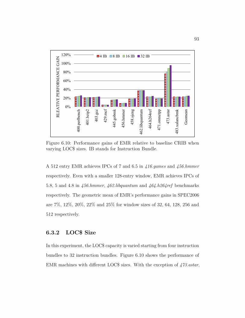
93
0%
20%
40%
60%
80%
100%
120%
400
.per
lben
ch
401.b
zip
2
403
.gcc
429
.mcf
44
5.g
obm
k
45
6.h
mm
er
45
8.s
jeng
46
2.l
ibq
uan
tum
464.h
264
ref
47
1.o
mnetp
p
47
3.a
star
48
3.x
alan
cbm
k
Geo
mea
n
RL
EA
TIV
E P
ER
FO
RM
AN
CE
GA
IN4 IB 8 IB 16 IB 32 IB
Figure 6.10: Performance gains of EMR relative to baseline CRIB whenvarying LOC$ sizes. IB stands for Instruction Bundle.
A 512 entry EMR achieves IPCs of 7 and 6.5 in 416.games and 456.hmmer
respectively. Even with a smaller 128-entry window, EMR achieves IPCs of
5.8, 5 and 4.8 in 456.hmmer, 462.libquantum and 464.h264ref benchmarks
respectively. The geometric mean of EMR’s performance gains in SPEC2006
are 7%, 12%, 20%, 22% and 25% for window sizes of 32, 64, 128, 256 and
512 respectively.
6.3.2 LOC$ Size
In this experiment, the LOC$ capacity is varied starting from four instruction
bundles to 32 instruction bundles. Figure 6.10 shows the performance of
EMR machines with different LOC$ sizes. With the exception of 473.astar,
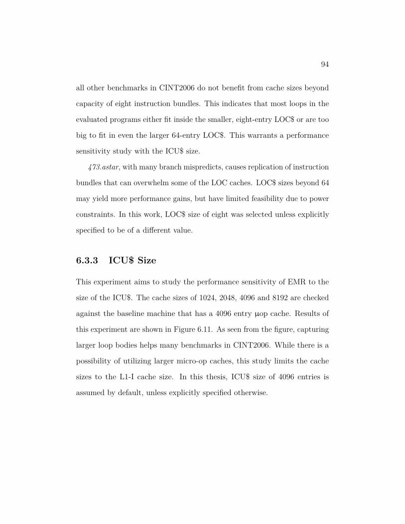
94
all other benchmarks in CINT2006 do not benefit from cache sizes beyond
capacity of eight instruction bundles. This indicates that most loops in the
evaluated programs either fit inside the smaller, eight-entry LOC$ or are too
big to fit in even the larger 64-entry LOC$. This warrants a performance
sensitivity study with the ICU$ size.
473.astar, with many branch mispredicts, causes replication of instruction
bundles that can overwhelm some of the LOC caches. LOC$ sizes beyond 64
may yield more performance gains, but have limited feasibility due to power
constraints. In this work, LOC$ size of eight was selected unless explicitly
specified to be of a different value.
6.3.3 ICU$ Size
This experiment aims to study the performance sensitivity of EMR to the
size of the ICU$. The cache sizes of 1024, 2048, 4096 and 8192 are checked
against the baseline machine that has a 4096 entry µop cache. Results of
this experiment are shown in Figure 6.11. As seen from the figure, capturing
larger loop bodies helps many benchmarks in CINT2006. While there is a
possibility of utilizing larger micro-op caches, this study limits the cache
sizes to the L1-I cache size. In this thesis, ICU$ size of 4096 entries is
assumed by default, unless explicitly specified otherwise.
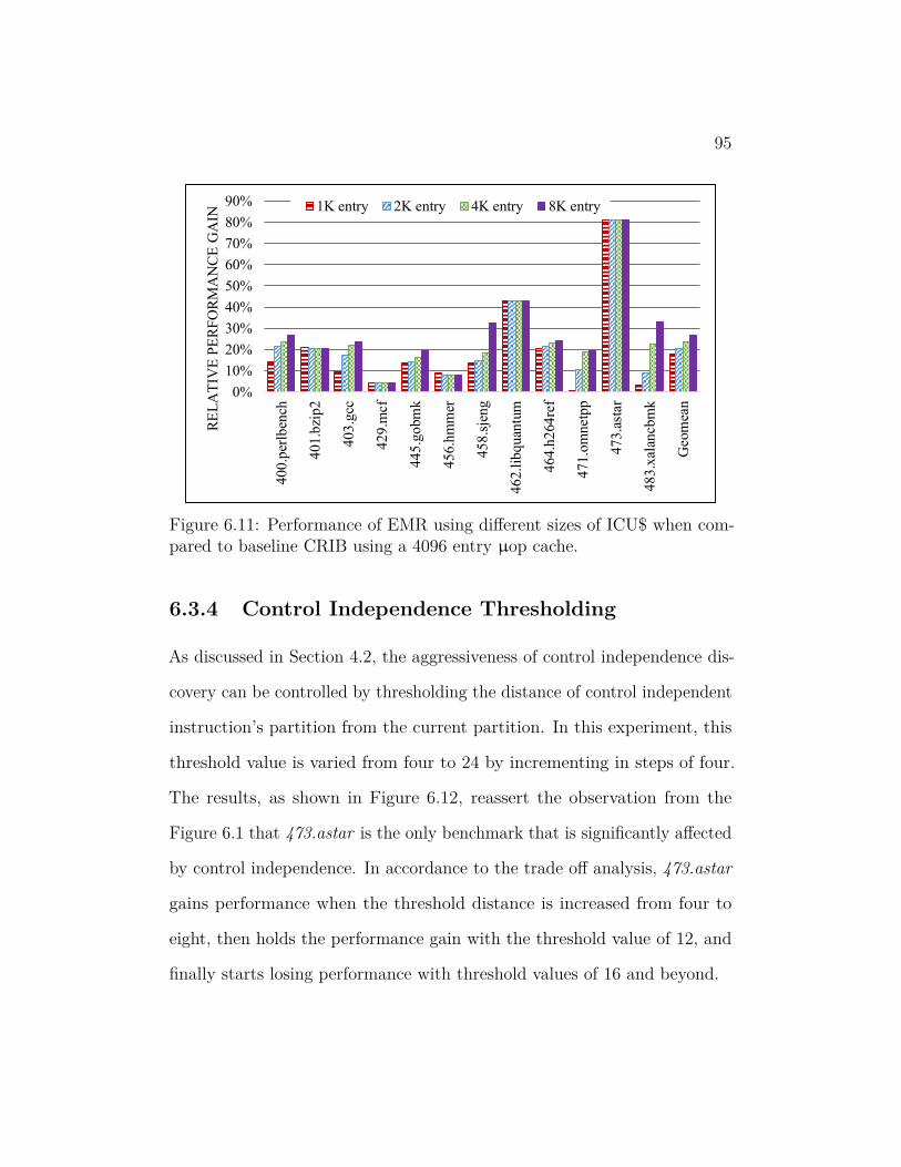
95
0%
10%
20%
30%
40%
50%
60%
70%
80%
90%
400
.per
lben
ch
401.b
zip
2
403
.gcc
429
.mcf
44
5.g
obm
k
45
6.h
mm
er
45
8.s
jeng
46
2.l
ibq
uan
tum
46
4.h
264
ref
47
1.o
mnetp
p
47
3.a
star
48
3.x
alan
cbm
k
Geo
mea
n
RE
LA
TIV
E P
ER
FO
RM
AN
CE
GA
IN1K entry 2K entry 4K entry 8K entry
Figure 6.11: Performance of EMR using different sizes of ICU$ when com-pared to baseline CRIB using a 4096 entry µop cache.
6.3.4 Control Independence Thresholding
As discussed in Section 4.2, the aggressiveness of control independence dis-
covery can be controlled by thresholding the distance of control independent
instruction’s partition from the current partition. In this experiment, this
threshold value is varied from four to 24 by incrementing in steps of four.
The results, as shown in Figure 6.12, reassert the observation from the
Figure 6.1 that 473.astar is the only benchmark that is significantly affected
by control independence. In accordance to the trade off analysis, 473.astar
gains performance when the threshold distance is increased from four to
eight, then holds the performance gain with the threshold value of 12, and
finally starts losing performance with threshold values of 16 and beyond.

96
0%
10%
20%
30%
40%
50%
60%
70%
80%
90%
400
.per
lben
ch
401.b
zip
2
403
.gcc
429
.mcf
44
5.g
obm
k
45
6.h
mm
er
45
8.s
jeng
46
2.l
ibq
uan
tum
464.h
264
ref
47
1.o
mnetp
p
47
3.a
star
48
3.x
alan
cbm
k
RE
LA
TIV
E P
ER
FO
RM
AN
CE
GA
INCI4 CI8 CI12 CI16 CI24
Figure 6.12: Split of instruction sources in EMR.
One of the main reasons that the negative performance trend is not
observed when increasing the threshold distance is due to the conservative
fill of the select address table as discussed in Section 4.2 of Chapter 4.
Irrespective of the threshold distance, if the target instruction is not found
in the select address table, it can not be selected. Throughout this thesis,
default assumption of the threshold value is 12.
6.3.5 ICU$ Access Delay
In most evaluations of EMR, ICU$ is assumed to be accessed in one cycle.
Note that this is just the ICU$ access time and not the ICU$ instruction
service time, which includes additional request and allocate latencies. ICU$
97
0%
10%
20%
30%
40%
50%
60%
70%
80%
90%
400
.per
lben
ch
401.b
zip
2
403
.gcc
429
.mcf
44
5.g
obm
k
45
6.h
mm
er
45
8.s
jeng
46
2.l
ibq
uan
tum
46
4.h
264
ref
47
1.o
mnetp
p
47
3.a
star
48
3.x
alan
cbm
k
Geo
mea
n
RE
LA
TIV
E P
ER
FO
RM
AN
CE
GA
INEMR_ICU$_d1 EMR_ICU$_d2 EMR_ICU$_d3
Figure 6.13: Performance gains of EMR over baseline CRIB when runningCINT2006 with varying ICU$ access time.
access of one cycle can be challenging in some processor designs as it can
limit clock speeds and reduce energy efficiency. In this experiment, the
performance of EMR is recorded when increasing the access delay of the
ICU$ from one to two, and to three cycles. Figure 6.13 shows the results
of this experiment. Note that in this experiment, the baseline CRIB’s µop
cache is still accessed in a single cycle across all the configurations.
Referring to the previous experiments, benchmarks like 471.omentpp,
483.xalancbmk and others that have high sensitivity to the LOC$ size are
impacted by the increased ICU$ delay. At the access delay of three, the
instruction service time from the ICU$ matches the instruction service time
from the µop cache in the baseline and thus the ICU$ has no advantage of
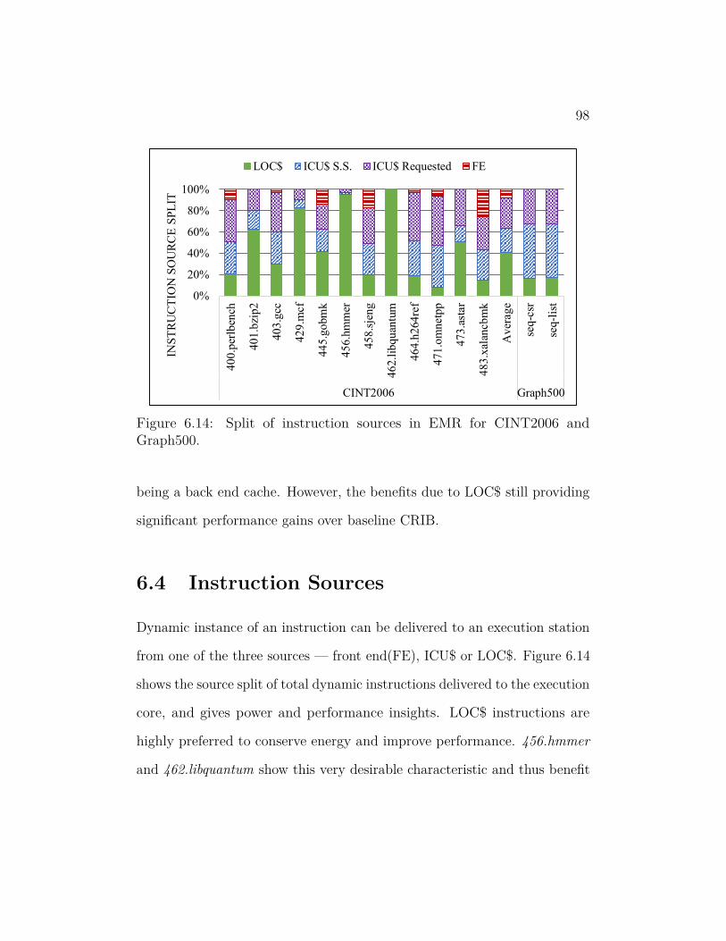
98
0%
20%
40%
60%
80%
100%
400.p
erlb
ench
40
1.b
zip2
403.g
cc
42
9.m
cf
44
5.g
obm
k
456
.hm
mer
45
8.s
jeng
462.l
ibqu
antu
m
464.h
264re
f
471.o
mnet
pp
473.a
star
483.x
alan
cbm
k
Av
erag
e
seq-c
sr
seq-l
ist
CINT2006 Graph500
INS
TR
UC
TIO
N S
OU
RC
E S
PL
ITLOC$ ICU$ S.S. ICU$ Requested FE
Figure 6.14: Split of instruction sources in EMR for CINT2006 andGraph500.
being a back end cache. However, the benefits due to LOC$ still providing
significant performance gains over baseline CRIB.
6.4 Instruction Sources
Dynamic instance of an instruction can be delivered to an execution station
from one of the three sources — front end(FE), ICU$ or LOC$. Figure 6.14
shows the source split of total dynamic instructions delivered to the execution
core, and gives power and performance insights. LOC$ instructions are
highly preferred to conserve energy and improve performance. 456.hmmer
and 462.libquantum show this very desirable characteristic and thus benefit

99
considerably from AID. ICU$ instructions take more energy for delivery
than the LOC$, but consume lower energy and deliver instructions faster
than front end instructions. Noticeably, most programs have large number
of instructions delivered from the back-end caches.
ICU$ accesses are broken down into two categories — ICU$ speculative
supply (annotated as ICU$ S.S. in the figure) and ICU$ requested. These
instructions are a "hit" in LOC$, but were speculatively inserted by the
ICU$. This classification helps understand the performance of benchmarks
like 464.h264ref, where the typical basic-block size is eight to 12 instructions
and multiple instruction bundles are speculatively serviced by the ICU$.
Though the graph in Figure 6.14 suggests poor LOC$ locality, the speculative
supplied instructions actually improve this locality and benefit AID. The
ICU$ requested instructions are the ones that are supplied to a partition on
an explicit request.
A few benchmarks, like 483.xalancbmk need instructions to be delivered
from the FE due to either cold, capacity or conflict misses in ICU$. Due to
the high penalty of redirecting the FE, it is only turned off when there is
significant confidence that it is not required.
Figure 6.15 shows the split of instruction sources for CFP2006 programs.
453.povray is the only benchmark with non-trivial number of front-end
instructions. All the programs seem to be captured well within the LOC
and ICU caches. 470.lbm is particularly interesting with almost a half way
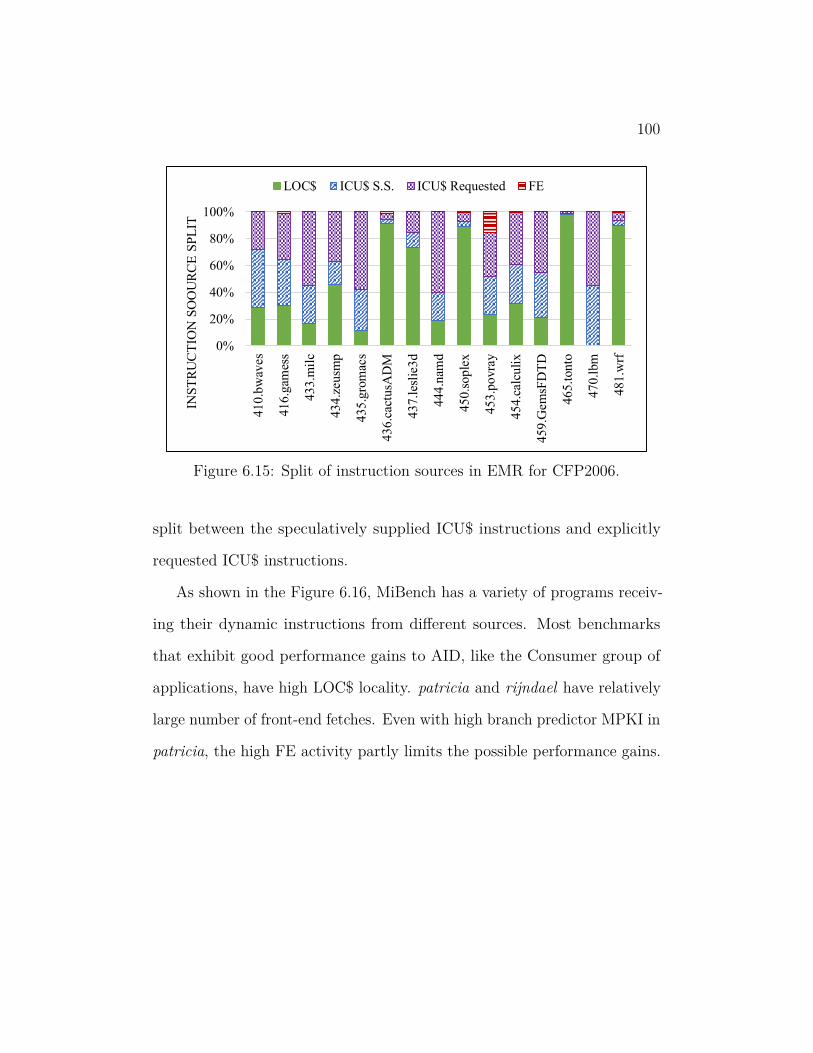
100
0%
20%
40%
60%
80%
100%
41
0.b
wav
es
41
6.g
ames
s
43
3.m
ilc
434
.zeu
smp
43
5.g
rom
acs
43
6.c
actu
sAD
M
437.l
esli
e3d
444.n
amd
450
.sople
x
45
3.p
ovra
y
45
4.c
alcu
lix
45
9.G
emsF
DT
D
465
.ton
to
470
.lbm
48
1.w
rf
INS
TR
UC
TIO
N S
OO
UR
CE
SP
LIT
LOC$ ICU$ S.S. ICU$ Requested FE
Figure 6.15: Split of instruction sources in EMR for CFP2006.
split between the speculatively supplied ICU$ instructions and explicitly
requested ICU$ instructions.
As shown in the Figure 6.16, MiBench has a variety of programs receiv-
ing their dynamic instructions from different sources. Most benchmarks
that exhibit good performance gains to AID, like the Consumer group of
applications, have high LOC$ locality. patricia and rijndael have relatively
large number of front-end fetches. Even with high branch predictor MPKI in
patricia, the high FE activity partly limits the possible performance gains.
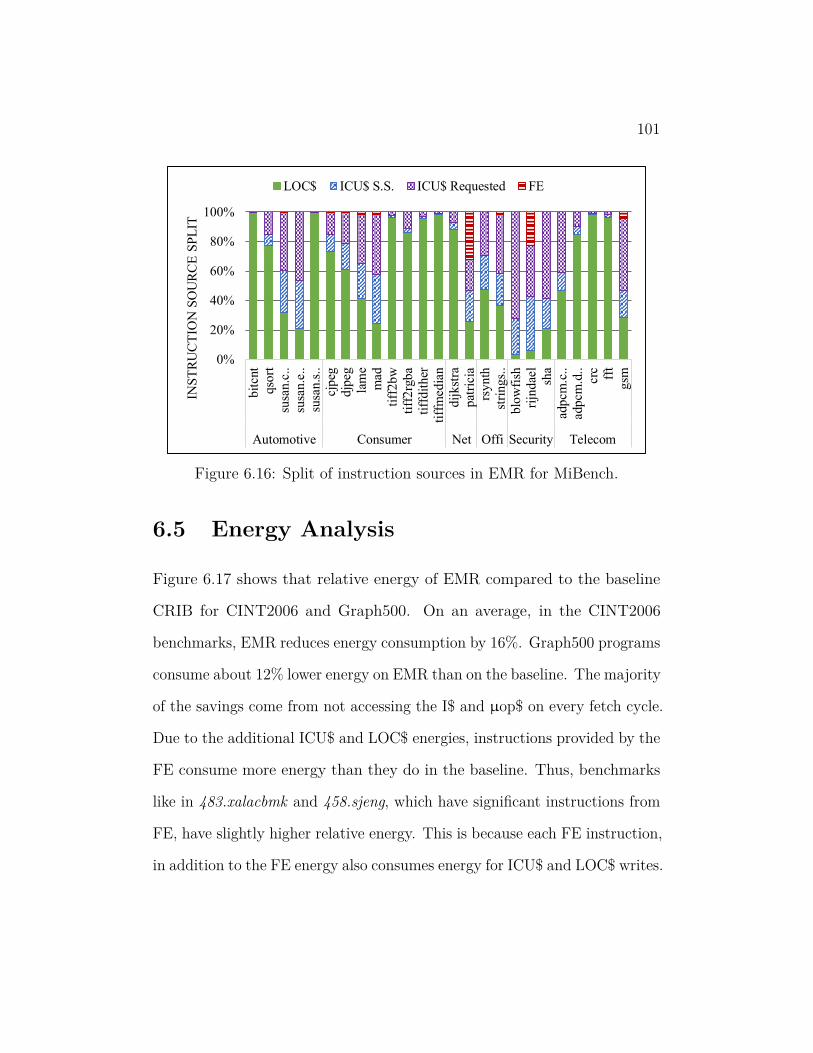
101
0%
20%
40%
60%
80%
100%
bit
cnt
qso
rt
susa
n.c
..
susa
n.e
..
susa
n.s
..
cjpeg
djp
eg
lam
e
mad
tiff
2b
w
tiff
2rg
ba
tiff
dit
her
tiff
med
ian
dij
kst
ra
pat
rici
a
rsynth
stri
ngs.
.
blo
wfi
sh
rijn
dae
l
sha
adp
cm.c
..
adp
cm.d
..
crc
fft
gsm
Automotive Consumer Net Offi Security Telecom
INS
TR
UC
TIO
N S
OU
RC
E S
PL
ITLOC$ ICU$ S.S. ICU$ Requested FE
Figure 6.16: Split of instruction sources in EMR for MiBench.
6.5 Energy Analysis
Figure 6.17 shows that relative energy of EMR compared to the baseline
CRIB for CINT2006 and Graph500. On an average, in the CINT2006
benchmarks, EMR reduces energy consumption by 16%. Graph500 programs
consume about 12% lower energy on EMR than on the baseline. The majority
of the savings come from not accessing the I$ and µop$ on every fetch cycle.
Due to the additional ICU$ and LOC$ energies, instructions provided by the
FE consume more energy than they do in the baseline. Thus, benchmarks
like in 483.xalacbmk and 458.sjeng, which have significant instructions from
FE, have slightly higher relative energy. This is because each FE instruction,
in addition to the FE energy also consumes energy for ICU$ and LOC$ writes.
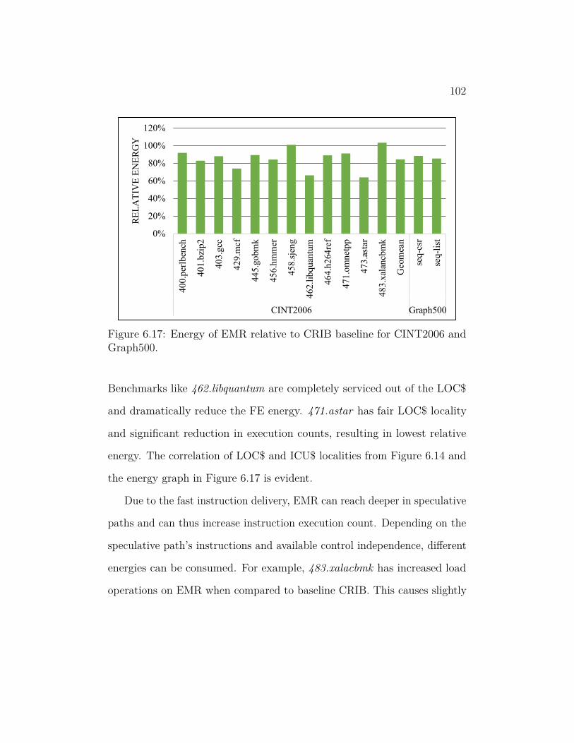
102
0%
20%
40%
60%
80%
100%
120%
400.p
erlb
ench
40
1.b
zip2
403.g
cc
42
9.m
cf
44
5.g
obm
k
456
.hm
mer
45
8.s
jeng
462.l
ibqu
antu
m
464.h
264re
f
471.o
mnet
pp
473.a
star
483.x
alan
cbm
k
Geo
mea
n
seq-c
sr
seq-l
ist
CINT2006 Graph500
RE
LA
TIV
E E
NE
RG
Y
Figure 6.17: Energy of EMR relative to CRIB baseline for CINT2006 andGraph500.
Benchmarks like 462.libquantum are completely serviced out of the LOC$
and dramatically reduce the FE energy. 471.astar has fair LOC$ locality
and significant reduction in execution counts, resulting in lowest relative
energy. The correlation of LOC$ and ICU$ localities from Figure 6.14 and
the energy graph in Figure 6.17 is evident.
Due to the fast instruction delivery, EMR can reach deeper in speculative
paths and can thus increase instruction execution count. Depending on the
speculative path’s instructions and available control independence, different
energies can be consumed. For example, 483.xalacbmk has increased load
operations on EMR when compared to baseline CRIB. This causes slightly

103
0%
10%
20%
30%
40%
50%
60%
70%
80%
90%
410
.bw
aves
41
6.g
ames
s
43
3.m
ilc
434.z
eusm
p
43
5.g
rom
acs
43
6.c
actu
sAD
M
437
.les
lie3
d
44
4.n
amd
450.s
ople
x
45
3.p
ovra
y
45
4.c
alcu
lix
45
9.G
emsF
DT
D
465
.ton
to
470.l
bm
481.w
rf
Geo
mea
n
RE
LA
TIV
E E
NE
RG
Y
Figure 6.18: Energy consumed by EMR as compared to baseline CRIB whenexecuting CFP2006 programs.
higher L1-D$ accesses which has significant impact on the consumed energy.
The high locality of instructions in the back end caches, as observed from
Figure 6.15, should result in energy savings for running CFP2006 benchmarks
on EMR. The results of the energy estimation tool, shown in Figure 6.18,
match this expectation. On an average, EMR uses only 75% of the energy
required by baseline CRIB to run CFP2006 benchmarks. 450.soplex uses
the lowest relative energy of 58% with 436.cactusADM following closely at
62%. Owing to high front end supplied instructions, energy savings from
executing 453.povray are lower on EMR. For benchmarks like 470.lbm, high
ICU$ accesses decrease the amount of energy that can be saved.

104
0%
20%
40%
60%
80%
100%
120%
bit
cnt
qso
rtsu
san.c
..su
san.e
..su
san.s
..cj
peg
djp
egla
me
mad
tiff
2b
wti
ff2rg
ba
tiff
dit
her
tiff
med
ian
dij
kst
rapat
rici
ars
ynth
stri
ng
s..
blo
wfi
shri
jndae
lsh
aad
pcm
.c..
adp
cm.d
..cr
cff
tgsm
Geo
mea
n
Automotive Consumer Net Offi Security Telecom O
RE
LA
TIV
E E
NE
RG
Y
Figure 6.19: Relative Energy of EMR as compared to the CRIB baselinewhen running MiBench programs.
As noted in the previous section, patricia and rijndael consume most
energy amongst the MiBench applications running on EMR. EMR consumes
4% and 9% more energy than the baseline crib to execute these programs.
However, there are many other programs in MiBench that offset this increase
with significant savings, leading to a geometric mean energy savings of 17%.
When run on EMR instead of baseline CRIB, tiff2rgba cuts down the energy
consumption by half.
Millions of instructions per second (MIPS) per watt, or millions of
instructions per joule, is a composite metric for evaluating performance and
energy consumption of a design. Figure 6.20, Figure 6.21 and Figure 6.22
show this metric for EMR relative to the baseline CRIB design for CINT2006,
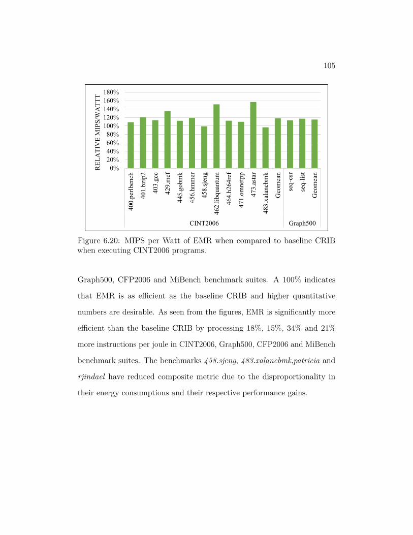
105
0%
20%
40%
60%
80%
100%
120%
140%
160%
180%
400
.per
lben
ch
401
.bzi
p2
403
.gcc
429
.mcf
445
.gob
mk
456
.hm
mer
458
.sje
ng
462
.lib
quan
tum
464
.h26
4re
f
471
.om
net
pp
473
.ast
ar
483
.xal
ancb
mk
Geo
mea
n
seq
-csr
seq
-lis
t
Geo
mea
n
CINT2006 Graph500
RE
LA
TIV
E M
IPS
/WA
TT
T
Figure 6.20: MIPS per Watt of EMR when compared to baseline CRIBwhen executing CINT2006 programs.
Graph500, CFP2006 and MiBench benchmark suites. A 100% indicates
that EMR is as efficient as the baseline CRIB and higher quantitative
numbers are desirable. As seen from the figures, EMR is significantly more
efficient than the baseline CRIB by processing 18%, 15%, 34% and 21%
more instructions per joule in CINT2006, Graph500, CFP2006 and MiBench
benchmark suites. The benchmarks 458.sjeng, 483.xalancbmk,patricia and
rjindael have reduced composite metric due to the disproportionality in
their energy consumptions and their respective performance gains.
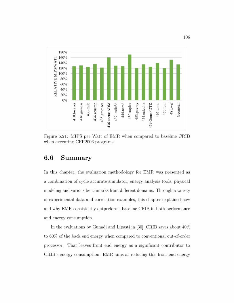
106
0%
20%
40%
60%
80%
100%
120%
140%
160%
180%
410
.bw
aves
416
.gam
ess
433
.mil
c
434
.zeu
smp
435
.gro
mac
s
436
.cac
tusA
DM
437
.les
lie3
d
444
.nam
d
450
.so
ple
x
453
.pov
ray
454
.cal
culi
x
459
.Gem
sFD
TD
465
.to
nto
470
.lb
m
481
.wrf
Geo
mea
n
RE
LA
TIV
E M
IPS
/WA
TT
Figure 6.21: MIPS per Watt of EMR when compared to baseline CRIBwhen executing CFP2006 programs.
6.6 Summary
In this chapter, the evaluation methodology for EMR was presented as
a combination of cycle accurate simulator, energy analysis tools, physical
modeling and various benchmarks from different domains. Through a variety
of experimental data and correlation examples, this chapter explained how
and why EMR consistently outperforms baseline CRIB in both performance
and energy consumption.
In the evaluations by Gunadi and Lipasti in [30], CRIB saves about 40%
to 60% of the back end energy when compared to conventional out-of-order
processor. That leaves front end energy as a significant contributor to
CRIB’s energy consumption. EMR aims at reducing this front end energy
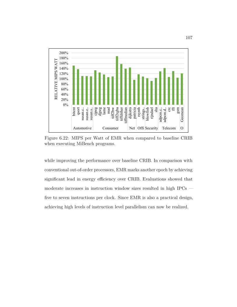
107
0%
20%
40%
60%
80%
100%
120%
140%
160%
180%
200%
bit
cnt
qso
rtsu
san.c
..su
san.e
..su
san.s
..cj
peg
djp
egla
me
mad
tiff
2bw
tiff
2rg
ba
tiff
dit
her
tiff
med
ian
dij
kst
rap
atri
cia
rsy
nth
stri
ng
s..
blo
wfi
shri
jndae
lsh
aad
pcm
.c..
adpcm
.d..
crc
fft
gsm
Geo
mea
n
Automotive Consumer Net Offi Security Telecom O
RE
LA
TIV
E M
IPS
/WA
TT
Figure 6.22: MIPS per Watt of EMR when compared to baseline CRIBwhen executing MiBench programs.
while improving the performance over baseline CRIB. In comparison with
conventional out-of-order processors, EMR marks another epoch by achieving
significant lead in energy efficiency over CRIB. Evaluations showed that
moderate increases in instruction window sizes resulted in high IPCs —
five to seven instructions per clock. Since EMR is also a practical design,
achieving high levels of instruction level parallelism can now be realized.

108
7 conclusionWith the end of Dennard scaling, increased core count and the inclusion
of uncore logic constrain the budget for a single processor core. With this
tightened budget, scaling traditional out-of-order cores can be limited due
to the exponential scaling of the architectural components. New paradigms
in computer architecture need to be explored to supply the performance
demands of future applications, while conforming to the allocated energy
budget. This dissertation work started with CRIB as the baseline with
an assumption that this practical architecture will see success in the near
future.
Advances in branch prediction have been instrumental in alleviating the
control dependence limitation on instruction level parallelism. However, the
existence of hard to predict branches and complexity limits seem to saturate
branch prediction accuracies. Additional performance from alleviating
control dependences can be achieved by either improving branch prediction
accuracies or by reducing the misprediction penalty. This thesis presented a
novel architecture, Express Misprediction Recovery, to reduce performance
and energy penalties associated with branch mispredictions.
EMR uses novel instruction delivery techniques to improve performance.
First, EMR dramatically reduces the execution-resume delay after a mispre-
diction by quickly providing the correct path instructions. Further more,
EMR uses a speculative next-index prediction to deliver more instructions

109
per cycle to the execution core and thus increases the Flynn’s bottleneck
limit on performance.
Program characteristics that are desirable for EMR are as follows:
1. Loops that can be captured within the location optimized caches of
EMR will reduce front end energy.
2. Low confidence branches in such loops can dramatically decrease the
execution resume delay.
3. Small, equally sized control dependent path of a low confidence branch
can improve the chances of exploiting control independence.
4. Since control independence in EMR does not affect the execution
resume delay, performance is impacted by the number of long latency
control independent instructions that are also data independent.
5. High instruction level parallelism provides more opportunities to utilize
amplified instruction delivery.
6. Loops with significant direct branches can result in wasteful pipeline
bubbles in the baseline and benefit EMR.
EMR is evaluated across multiple benchmarks using cycle accurate
simulators to observe the machine characteristics and explore the design
space. Overall, EMR outperforms baseline CRIB by 23%, 20%, 10.5% and
4% in CINT2006, MiBench, Graph500 and CFP2006 respectively. This

110
performance gains are due to a combination of In-place fetch, In-place
control independence and amplified instruction delivery. In-place fetch
boosts performance by reducing the execution resume delay after a branch
mispredict. The long latency control independent data independent opera-
tions are utilized by the In-place control independence to provide additional
performance gains. Amplified instruction delivery increases the theoretical
limits on the instructions committed per clock, thus providing additional
performance.
In addition to boosting performance, EMR also saves 16%, 17%, 13% and
25% of the baseline energy when running CINT2006, MiBench, Graph500
and CFP2006 respectively. As we scale up the window sizes, EMR can, with
its amplified instruction delivery, commit up to seven µops per cycle.
7.1 Future Work
During the course of this research, new frontiers seemed worthwhile of
exploration in the future. Hardware specific compiler optimizations have
traditionally improved usage of certain processor features and EMR may
also benefit from such compiler optimizations. Other research ideas included
extending the EMR architecture to enable eager execution, architectural
changes to CRIB to make it implementable and value based architectural
techniques.
111
7.1.1 Compiler Support for EMR
Compiler support can improve energy and performance of EMR. Knowledge
of the back end caches can be used to optimize loops in a way to minimize
front end activity. In the presented version of EMR, control independence can
be realized only when the incorrectly predicted path is longer than the correct
path. By balancing the number of instructions between pre-dominator and
post-dominator instructions, such a restriction can be avoided to enable
more control independence opportunities.
Knowledge of LOC$ size can be used by a compiler to optimize code
for high LOC$ locality. Effective capacities of back end caches and EMR
partitions can be optimized by generating code that can be dispatched as
groups of four.
7.1.2 Eager Execution
Eager execution in EMR would require an additional set of latches across
each partition to hold the speculative state. If a branch is not resolved and
the next partition has finished executing all the instructions, it can latch its
speculative state and start executing the alternate path. A special ability
with EMR is that eager execution can proceed at partition granularity and it
is likely that alternate path instructions are delivered from the LOC caches.
Possibly the biggest challenge is the performance expectation from eager
execution. Given that EMR already benefits from reducing execution-resume

112
time, and utilizes control independence, an accurate estimation has to be
made for the expected performance gains due to eager execution.
Other challenges are to look out for cases when the unresolved branch
is in the middle of a partition with younger data-generating instructions
within the same partition. Policies need to be explored on the course of
action when required instructions are not available in the back end caches.
To abide by the power constraints, eager execution is probably done for a
select set of branches [53]. Detection of such branches can be done by some
form of prediction.
7.1.3 Impediments to CRIB’s Implementation
Discussions with different computer architects and engineers have surfaced
some practical issues with CRIB. One major complaint is that the existing
data path can not scale well with increasing architectural registers. The
latest ARM 64-bit ISA has 32 architectural registers. This requires 2048
interconnection wires between each execution station.
Moving the complex router logic up to the partition level can largely
address this problem. Other solutions may exist to achieve this goal, like
exploring novel layout techniques using multiple metal layers.

113
7.1.4 Value Based Architectural Techniques
Many architectural optimizations are very simple with CRIB as the data is
available during the schedule time. Long latency instructions, like floating
point adds, can be avoided if one of the inputs results in elimination. Other
architectural techniques using partial instruction and data memoization
are also practical in CRIB due its inherent ability to repair dependencies
in-place.
114
bibliography[1] M. Agarwal et al. “Fetch-Criticality Reduction through Control
Independence”. In: Computer Architecture, 2008. ISCA ’08. 35thInternational Symposium on. 2008, pp. 13–24. doi: 10.1109/ISCA.2008.39.
[2] Pritpal S. Ahuja et al. “Multipath Execution: Opportunities andLimits”. In: Proceedings of the 12th International Conference onSupercomputing. ICS ’98. Melbourne, Australia: ACM, 1998, pp. 101–108. isbn: 0-89791-998-X. doi: 10.1145/277830.277854. url: http://doi.acm.org/10.1145/277830.277854.
[3] Haitham Akkary and Michael A. Driscoll. “A Dynamic Multithread-ing Processor”. In: Proceedings of the 31st Annual ACM/IEEE In-ternational Symposium on Microarchitecture. MICRO 31. Dallas,Texas, USA: IEEE Computer Society Press, 1998, pp. 226–236. isbn:1-58113-016-3. url: http : / / dl . acm . org / citation . cfm ? id =290940.290988.
[4] Ahmed S. Al-Zawawi et al. “Transparent Control Independence(TCI)”. In: Proceedings of the 34th Annual International Symposiumon Computer Architecture. ISCA ’07. San Diego, California, USA:ACM, 2007, pp. 448–459. isbn: 978-1-59593-706-3. doi: 10.1145/1250662.1250717. url: http://doi.acm.org/10.1145/1250662.1250717.
[5] D. W. Anderson, F. J. Sparacio, and R. M. Tomasulo. “The IBM Sys-tem/360 Model 91: Machine Philosophy and Instruction-Handling”.In: IBM Journal of Research and Development 11.1 (1967), pp. 8–24.issn: 0018-8646. doi: 10.1147/rd.111.0008.
[6] D. Bhandarkar and J. Ding. “Performance characterization of thePentium Pro processor”. In: High-Performance Computer Architec-ture, 1997., Third International Symposium on. 1997, pp. 288–297.doi: 10.1109/HPCA.1997.569689.
[7] Nathan Binkert et al. “The Gem5 Simulator”. In: SIGARCH Comput.Archit. News 39.2 (Aug. 2011), pp. 1–7. issn: 0163-5964. doi: 10.1145/2024716.2024718. url: http://doi.acm.org/10.1145/2024716.2024718.
115
[8] Werner Buchholz. Planning a Computer System: Project Stretch.Hightstown, NJ, USA: McGraw-Hill, Inc., 1962. isbn: B0000CLCYO.
[9] Mike Butler. “AMD "Bulldozer" Core-a new approach to multi-threaded compute performance for maximum efficiency and through-put”. In: IEEE HotChips Symposium on High-Performance Chips(HotChips 2010). 2010.
[10] B. Calder and D. Grunwald. “Fast and accurate instruction fetch andbranch prediction”. In: Computer Architecture, 1994., Proceedingsthe 21st Annual International Symposium on. 1994, pp. 2–11. doi:10.1109/ISCA.1994.288166.
[11] Po-Yung Chang, Marius Evers, and YaleN. Patt. “Improving branchprediction accuracy by reducing pattern history table interference”.English. In: International Journal of Parallel Programming 25.5(1997), pp. 339–362. issn: 0885-7458. doi: 10.1007/BF02699882.url: http://dx.doi.org/10.1007/BF02699882.
[12] Po-Yung Chang et al. “Branch Classification: A New Mechanism forImproving Branch Predictor Performance”. In: Proceedings of the27th Annual International Symposium on Microarchitecture. MICRO27. San Jose, California, USA: ACM, 1994, pp. 22–31. isbn: 0-89791-707-3. doi: 10.1145/192724.192727. url: http://doi.acm.org/10.1145/192724.192727.
[13] Chen-Yong Cher and T. N. Vijaykumar. “Skipper: A Microarchitec-ture for Exploiting Control-flow Independence”. In: Proceedings ofthe 34th Annual ACM/IEEE International Symposium on Microar-chitecture. MICRO 34. Austin, Texas: IEEE Computer Society, 2001,pp. 4–15. isbn: 0-7695-1369-7. url: http://dl.acm.org/citation.cfm?id=563998.564002.
[14] Yuan Chou, Jason Fung, and John Paul Shen. “Reducing BranchMisprediction Penalties via Dynamic Control Independence Detec-tion”. In: Proceedings of the 13th International Conference on Su-percomputing. ICS ’99. Rhodes, Greece: ACM, 1999, pp. 109–118.isbn: 1-58113-164-X. doi: 10.1145/305138.305175. url: http://doi.acm.org/10.1145/305138.305175.

116
[15] Yuan Chou, Jason Fung, and John Paul Shen. “Reducing BranchMisprediction Penalties via Dynamic Control Independence Detec-tion”. In: Proceedings of the 13th International Conference on Su-percomputing. ICS ’99. Rhodes, Greece: ACM, 1999, pp. 109–118.isbn: 1-58113-164-X. doi: 10.1145/305138.305175. url: http://doi.acm.org/10.1145/305138.305175.
[16] Niket K. Choudhary et al. “FabScalar: Composing Synthesizable RTLDesigns of Arbitrary Cores Within a Canonical Superscalar Tem-plate”. In: Proceedings of the 38th Annual International Symposiumon Computer Architecture. ISCA ’11. San Jose, California, USA: ACM,2011, pp. 11–22. isbn: 978-1-4503-0472-6. doi: 10.1145/2000064.2000067. url: http://doi.acm.org/10.1145/2000064.2000067.
[17] Weihaw Chuang and Brad Calder. “Predicate Prediction for Effi-cient Out-of-order Execution”. In: Proceedings of the 17th AnnualInternational Conference on Supercomputing. ICS ’03. San Fran-cisco, CA, USA: ACM, 2003, pp. 183–192. isbn: 1-58113-733-8. doi:10.1145/782814.782840. url: http://doi.acm.org/10.1145/782814.782840.
[18] L. Codrescu et al. “Qualcomm Hexagon DSP: An Architecture Opti-mized for Mobile Multimedia and Communications”. In: Hot Chips,2013.
[19] Lynn Conway. IBM-ACS: Reminiscences and Lessons Learned froma 1960’s Supercomputer Project. Springer, 2011.
[20] ARM Cortex. “a9 processor”. In: URL: http://www. arm. com/products/processors/cortex-a/cortex-a9. php.[Accessed 6 January 2014] (2011).
[21] A. N. Eden and T. Mudge. “The YAGS Branch Prediction Scheme”.In: Proceedings of the 31st Annual ACM/IEEE International Sympo-sium on Microarchitecture. MICRO 31. Dallas, Texas, USA: IEEEComputer Society Press, 1998, pp. 69–77. isbn: 1-58113-016-3. url:http://dl.acm.org/citation.cfm?id=290940.290962.
[22] Equator. “MAP1000 unfolds at Equator”. In: Microprocessor Report.1998.
117
[23] Marius Evers, Po-Yung Chang, and Yale N. Patt. “Using HybridBranch Predictors to Improve Branch Prediction Accuracy in thePresence of Context Switches”. In: Proceedings of the 23rd Annual In-ternational Symposium on Computer Architecture. ISCA ’96. Philadel-phia, Pennsylvania, USA: ACM, 1996, pp. 3–11. isbn: 0-89791-786-3.doi: 10.1145/232973.232975. url: http://doi.acm.org/10.1145/232973.232975.
[24] Paolo Faraboschi et al. “Lx: a technology platform for customizableVLIW embedded processing”. In: ISCA-27. 2000.
[25] Jose Fridman and Zvi Greenfield. “The TigerSHARC DSP Architec-ture”. In: IEEE Micro (2000).
[26] Amit Gandhi, Haitham Akkary, and Srikanth T. Srinivasan. “Reduc-ing Branch Misprediction Penalty via Selective Branch Recovery”.In: Proceedings of the 10th International Symposium on High Perfor-mance Computer Architecture. HPCA ’04. Washington, DC, USA:IEEE Computer Society, 2004, pp. 254–. isbn: 0-7695-2053-7. doi:10.1109/HPCA.2004.10004. url: http://dx.doi.org/10.1109/HPCA.2004.10004.
[27] J.S. Gardner. “CEVA Exposes DSP Six Pack”. In: MicroprocessorReport, March 2012.
[28] Simcha Gochman et al. “Introduction to Intel Core Duo ProcessorArchitecture.” In: Intel Technology Journal 10.2 (2006).
[29] G. F. Grohoski. “Machine organization of the IBM RISC System/6000processor”. In: IBM Journal of Research and Development 34.1 (1990),pp. 37–58. issn: 0018-8646. doi: 10.1147/rd.341.0037.
[30] Erika Gunadi and Mikko H. Lipasti. “CRIB: Consolidated Rename,Issue, and Bypass”. In: Proceedings of the 38th Annual InternationalSymposium on Computer Architecture. ISCA ’11. San Jose, California,USA: ACM, 2011, pp. 23–32. isbn: 978-1-4503-0472-6. doi: 10.1145/2000064.2000068. url: http://doi.acm.org/10.1145/2000064.2000068.
[31] M. R. Guthaus et al. “MiBench: A Free, Commercially Representa-tive Embedded Benchmark Suite”. In: Proceedings of the WorkloadCharacterization, 2001. WWC-4. 2001 IEEE International Workshop.WWC ’01. Washington, DC, USA: IEEE Computer Society, 2001,

118
pp. 3–14. isbn: 0-7803-7315-4. doi: 10.1109/WWC.2001.15. url:http://dx.doi.org/10.1109/WWC.2001.15.
[32] Linley Gwennap. “Hal reveals multichip SPARC processor”. In: Mi-croprocessor Report 9.3 (1995), pp. 1–11.
[33] Linley Gwennap. “Sandy Bridge spans generations”. In: Microproces-sor Report 9.27 (2010), pp. 10–01.
[34] Per Hammarlund et al. “Haswell: The Fourth-Generation Intel CoreProcessor”. In: Micro, IEEE 34.2 (2014), pp. 6–20. issn: 0272-1732.doi: 10.1109/MM.2014.10.
[35] Mitchell Hayenga, Vignyan Reddy Kothinti Naresh, and Mikko HLipasti. “Revolver: Processor Architecture for Power Efficient LoopExecution”. In: HPCA-20. 2014.
[36] Timothy H. Heil and James. E. Smith. Selective Dual Path Execution.Tech. rep. University of Wisconsin — Madison, 1996.
[37] John L Hennessy and David A Patterson. Computer architecture: aquantitative approach. Elsevier, 2012.
[38] John L. Henning. “SPEC CPU2006 Benchmark Descriptions”. In:SIGARCH Comput. Archit. News 34.4 (Sept. 2006), pp. 1–17. issn:0163-5964. doi: 10.1145/1186736.1186737. url: http://doi.acm.org/10.1145/1186736.1186737.
[39] D.S. Henry, B.C. Kuszmaul, and V. Viswanath. “The Ultrascalarprocessor-an asymptotically scalable superscalar microarchitecture”.In: Advanced Research in VLSI, 1999. Proceedings. 20th AnniversaryConference on. 1999, pp. 256–273. doi: 10.1109/ARVLSI.1999.756053.
[40] M.D. Hill and M.R. Marty. “Amdahl’s Law in the Multicore Era”.In: Computer 41.7 (2008), pp. 33 –38.
[41] Andrew D. Hilton and Amir Roth. “Ginger: Control IndependenceUsing Tag Rewriting”. In: Proceedings of the 34th Annual Interna-tional Symposium on Computer Architecture. ISCA ’07. San Diego,California, USA: ACM, 2007, pp. 436–447. isbn: 978-1-59593-706-3.doi: 10.1145/1250662.1250716. url: http://doi.acm.org/10.1145/1250662.1250716.
119
[42] P. Y T Hsu and E. S. Davidson. “Highly Concurrent Scalar Process-ing”. In: Proceedings of the 13th Annual International Symposiumon Computer Architecture. ISCA ’86. Tokyo, Japan: IEEE ComputerSociety Press, 1986, pp. 386–395. isbn: 0-8186-0719-X. url: http://dl.acm.org/citation.cfm?id=17407.17401.
[43] Roland N. Ibbett. “The MU5 instruction pipeline”. In: The ComputerJournal 15 (1 1972), pp. 42–50.
[44] Texas Instrucments Inc. “TMS320C62x/67x CPU and InstructionSet Reference Guide”. In: 1998.
[45] Texas Instruments. “TMS320C6745/C6747 Fixed/Floating- pointdigital signal processors (Rev.D)”. In: (2010).
[46] E. Jacobsen, E. Rotenberg, and J.E. Smith. “Assigning confidence toconditional branch predictions”. In: Microarchitecture, 1996. MICRO-29.Proceedings of the 29th Annual IEEE/ACM International Sympo-sium on. 1996, pp. 142–152. doi: 10.1109/MICRO.1996.566457.
[47] D.A Jimenez and C. Lin. “Dynamic branch prediction with percep-trons”. In: High-Performance Computer Architecture, 2001. HPCA.The Seventh International Symposium on. 2001, pp. 197–206. doi:10.1109/HPCA.2001.903263.
[48] Daniel A. Jiménez and Calvin Lin. “Neural Methods for DynamicBranch Prediction”. In: ACM Trans. Comput. Syst. 20.4 (Nov. 2002),pp. 369–397. issn: 0734-2071. doi: 10.1145/571637.571639. url:http://doi.acm.org/10.1145/571637.571639.
[49] David R. Kaeli and Philip G. Emma. “Branch History Table Pre-diction of Moving Target Branches Due to Subroutine Returns”. In:Proceedings of the 18th Annual International Symposium on Com-puter Architecture. ISCA ’91. Toronto, Ontario, Canada: ACM, 1991,pp. 34–42. isbn: 0-89791-394-9. doi: 10.1145/115952.115957. url:http://doi.acm.org/10.1145/115952.115957.
[50] David Kanter. “Silvermont, Intel’s Low Power Architecture”. In:URL:http://www.realworldtech.com/silvermont (2013).
[51] R. E. Kessler. “The Alpha 21264 microprocessor”. In: Micro, IEEE19.2 (1999), pp. 24–36. issn: 0272-1732. doi: 10.1109/40.755465.
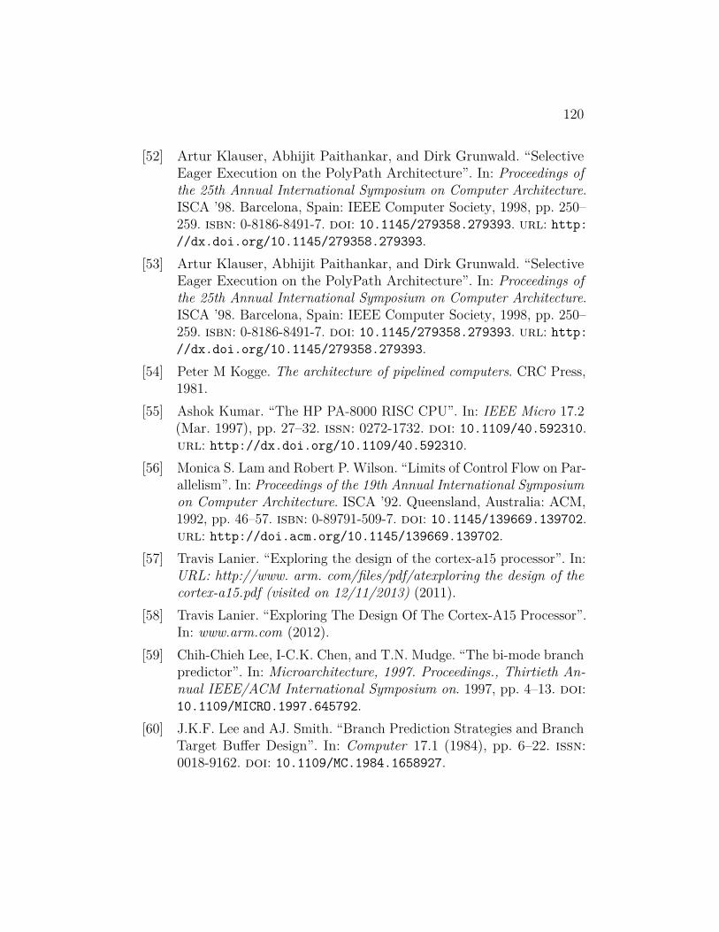
120
[52] Artur Klauser, Abhijit Paithankar, and Dirk Grunwald. “SelectiveEager Execution on the PolyPath Architecture”. In: Proceedings ofthe 25th Annual International Symposium on Computer Architecture.ISCA ’98. Barcelona, Spain: IEEE Computer Society, 1998, pp. 250–259. isbn: 0-8186-8491-7. doi: 10.1145/279358.279393. url: http://dx.doi.org/10.1145/279358.279393.
[53] Artur Klauser, Abhijit Paithankar, and Dirk Grunwald. “SelectiveEager Execution on the PolyPath Architecture”. In: Proceedings ofthe 25th Annual International Symposium on Computer Architecture.ISCA ’98. Barcelona, Spain: IEEE Computer Society, 1998, pp. 250–259. isbn: 0-8186-8491-7. doi: 10.1145/279358.279393. url: http://dx.doi.org/10.1145/279358.279393.
[54] Peter M Kogge. The architecture of pipelined computers. CRC Press,1981.
[55] Ashok Kumar. “The HP PA-8000 RISC CPU”. In: IEEE Micro 17.2(Mar. 1997), pp. 27–32. issn: 0272-1732. doi: 10.1109/40.592310.url: http://dx.doi.org/10.1109/40.592310.
[56] Monica S. Lam and Robert P. Wilson. “Limits of Control Flow on Par-allelism”. In: Proceedings of the 19th Annual International Symposiumon Computer Architecture. ISCA ’92. Queensland, Australia: ACM,1992, pp. 46–57. isbn: 0-89791-509-7. doi: 10.1145/139669.139702.url: http://doi.acm.org/10.1145/139669.139702.
[57] Travis Lanier. “Exploring the design of the cortex-a15 processor”. In:URL: http://www. arm. com/files/pdf/atexploring the design of thecortex-a15.pdf (visited on 12/11/2013) (2011).
[58] Travis Lanier. “Exploring The Design Of The Cortex-A15 Processor”.In: www.arm.com (2012).
[59] Chih-Chieh Lee, I-C.K. Chen, and T.N. Mudge. “The bi-mode branchpredictor”. In: Microarchitecture, 1997. Proceedings., Thirtieth An-nual IEEE/ACM International Symposium on. 1997, pp. 4–13. doi:10.1109/MICRO.1997.645792.
[60] J.K.F. Lee and AJ. Smith. “Branch Prediction Strategies and BranchTarget Buffer Design”. In: Computer 17.1 (1984), pp. 6–22. issn:0018-9162. doi: 10.1109/MC.1984.1658927.
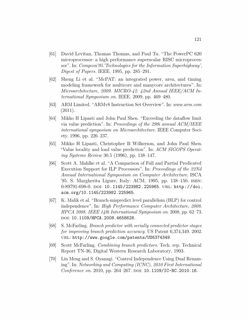
121
[61] David Levitan, Thomas Thomas, and Paul Tu. “The PowerPC 620microprocessor: a high performance superscalar RISC microproces-sor”. In: Compcon’95.’Technologies for the Information Superhighway’,Digest of Papers. IEEE. 1995, pp. 285–291.
[62] Sheng Li et al. “McPAT: an integrated power, area, and timingmodeling framework for multicore and manycore architectures”. In:Microarchitecture, 2009. MICRO-42. 42nd Annual IEEE/ACM In-ternational Symposium on. IEEE. 2009, pp. 469–480.
[63] ARM Limited. “ARMv8 Instruction Set Overview”. In: www.arm.com(2011).
[64] Mikko H Lipasti and John Paul Shen. “Exceeding the dataflow limitvia value prediction”. In: Proceedings of the 29th annual ACM/IEEEinternational symposium on Microarchitecture. IEEE Computer Soci-ety. 1996, pp. 226–237.
[65] Mikko H Lipasti, Christopher B Wilkerson, and John Paul Shen.“Value locality and load value prediction”. In: ACM SIGOPS Operat-ing Systems Review 30.5 (1996), pp. 138–147.
[66] Scott A. Mahlke et al. “A Comparison of Full and Partial PredicatedExecution Support for ILP Processors”. In: Proceedings of the 22NdAnnual International Symposium on Computer Architecture. ISCA’95. S. Margherita Ligure, Italy: ACM, 1995, pp. 138–150. isbn:0-89791-698-0. doi: 10.1145/223982.225965. url: http://doi.acm.org/10.1145/223982.225965.
[67] K. Malik et al. “Branch-mispredict level parallelism (BLP) for controlindependence”. In: High Performance Computer Architecture, 2008.HPCA 2008. IEEE 14th International Symposium on. 2008, pp. 62–73.doi: 10.1109/HPCA.2008.4658628.
[68] S. McFarling. Branch predictor with serially connected predictor stagesfor improving branch prediction accuracy. US Patent 6,374,349. 2002.url: http://www.google.com/patents/US6374349.
[69] Scott McFarling. Combining branch predictors. Tech. rep. TechnicalReport TN-36, Digital Western Research Laboratory, 1993.
[70] Lin Meng and S. Oyanagi. “Control Independence Using Dual Renam-ing”. In: Networking and Computing (ICNC), 2010 First InternationalConference on. 2010, pp. 264–267. doi: 10.1109/IC-NC.2010.16.

122
[71] C.J. Michael and D.M. Koppelman. “The effects on branch predictionwhen utilizing control independence”. In: Parallel Distributed Process-ing, Workshops and Phd Forum (IPDPSW), 2010 IEEE InternationalSymposium on. 2010, pp. 1–4. doi: 10.1109/IPDPSW.2010.5470794.
[72] Pierre Michaud. “A PPM-like, tag-based branch predictor”. In: Jour-nal of Instruction Level Parallelism 7.1 (2005), pp. 1–10.
[73] Pierre Michaud, André Seznec, and Richard Uhlig. “Trading Con-flict and Capacity Aliasing in Conditional Branch Predictors”. In:Proceedings of the 24th Annual International Symposium on Com-puter Architecture. ISCA ’97. Denver, Colorado, USA: ACM, 1997,pp. 292–303. isbn: 0-89791-901-7. doi: 10.1145/264107.264211.url: http://doi.acm.org/10.1145/264107.264211.
[74] Naveen Muralimanohar, Rajeev Balasubramonian, and Norman PJouppi. “CACTI 6.0: A tool to understand large caches”. In: Univer-sity of Utah and Hewlett Packard Laboratories, Tech. Rep (2009).
[75] Richard C Murphy et al. “Introducing the graph 500”. In: Cray User‘sGroup (CUG) (2010).
[76] Ravi Nair. “Dynamic Path-based Branch Correlation”. In: Proceedingsof the 28th Annual International Symposium on Microarchitecture.MICRO 28. Ann Arbor, Michigan, USA: IEEE Computer SocietyPress, 1995, pp. 15–23. isbn: 0-8186-7349-4. url: http://dl.acm.org/citation.cfm?id=225160.225168.
[77] NVIDIA. “NVIDIA Tegra 4 Family CPU Architecture”. In: (2013).url: http://www.nvidia.com/object/white-papers.html.
[78] R. R. Oehler and R. D. Groves. “IBM RISC System/6000 ProcessorArchitecture”. In: IBM J. Res. Dev. 34.1 (Jan. 1990), pp. 23–36. issn:0018-8646. doi: 10.1147/rd.341.0023. url: http://dx.doi.org/10.1147/rd.341.0023.
[79] C. Ozturk and R. Sendag. “An analysis of hard to predict branches”.In: Performance Analysis of Systems Software (ISPASS), 2010 IEEEInternational Symposium on. 2010, pp. 213–222. doi: 10.1109/ISPASS.2010.5452016.
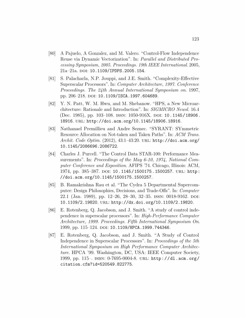
123
[80] A Pajuelo, A Gonzalez, and M. Valero. “Control-Flow IndependenceReuse via Dynamic Vectorization”. In: Parallel and Distributed Pro-cessing Symposium, 2005. Proceedings. 19th IEEE International. 2005,21a–21a. doi: 10.1109/IPDPS.2005.154.
[81] S. Palacharla, N.P. Jouppi, and J.E. Smith. “Complexity-EffectiveSuperscalar Processors”. In: Computer Architecture, 1997. ConferenceProceedings. The 24th Annual International Symposium on. 1997,pp. 206–218. doi: 10.1109/ISCA.1997.604689.
[82] Y. N. Patt, W. M. Hwu, and M. Shebanow. “HPS, a New Microar-chitecture: Rationale and Introduction”. In: SIGMICRO Newsl. 16.4(Dec. 1985), pp. 103–108. issn: 1050-916X. doi: 10.1145/18906.18916. url: http://doi.acm.org/10.1145/18906.18916.
[83] Nathanael Premillieu and Andre Seznec. “SYRANT: SYmmetricResource Allocation on Not-taken and Taken Paths”. In: ACM Trans.Archit. Code Optim. (2012), 43:1–43:20. url: http://doi.acm.org/10.1145/2086696.2086722.
[84] Charles J. Purcell. “The Control Data STAR-100: Performance Mea-surements”. In: Proceedings of the May 6-10, 1974, National Com-puter Conference and Exposition. AFIPS ’74. Chicago, Illinois: ACM,1974, pp. 385–387. doi: 10.1145/1500175.1500257. url: http://doi.acm.org/10.1145/1500175.1500257.
[85] B. Ramakrishna Rau et al. “The Cydra 5 Departmental Supercom-puter: Design Philosophies, Decisions, and Trade-Offs”. In: Computer22.1 (Jan. 1989), pp. 12–26, 28–30, 32–35. issn: 0018-9162. doi:10.1109/2.19820. url: http://dx.doi.org/10.1109/2.19820.
[86] E. Rotenberg, Q. Jacobson, and J. Smith. “A study of control inde-pendence in superscalar processors”. In: High-Performance ComputerArchitecture, 1999. Proceedings. Fifth International Symposium On.1999, pp. 115–124. doi: 10.1109/HPCA.1999.744346.
[87] E. Rotenberg, Q. Jacobson, and J. Smith. “A Study of ControlIndependence in Superscalar Processors”. In: Proceedings of the 5thInternational Symposium on High Performance Computer Architec-ture. HPCA ’99. Washington, DC, USA: IEEE Computer Society,1999, pp. 115–. isbn: 0-7695-0004-8. url: http://dl.acm.org/citation.cfm?id=520549.822775.

124
[88] Eric Rotenberg and Jim Smith. “Control Independence in TraceProcessors”. In: Proceedings of the 32Nd Annual ACM/IEEE Inter-national Symposium on Microarchitecture. MICRO 32. Haifa, Israel:IEEE Computer Society, 1999, pp. 4–15. isbn: 0-7695-0437-X. url:http://dl.acm.org/citation.cfm?id=320080.320084.
[89] Eric Rotenberg et al. “Trace Processors”. In: Proceedings of the 30thAnnual ACM/IEEE International Symposium on Microarchitecture.MICRO 30. Research Triangle Park, North Carolina, USA: IEEEComputer Society, 1997, pp. 138–148. isbn: 0-8186-7977-8. url:http://dl.acm.org/citation.cfm?id=266800.266814.
[90] C. Rowen et al. “The World’s Fastest DSP Core:Breaking the 100GMAC/s Barrier”. In: Hot Chips, 2011.
[91] Richard M. Russell. “The CRAY-1 Computer System”. In: Commun.ACM 21.1 (Jan. 1978), pp. 63–72. issn: 0001-0782. doi: 10.1145/359327.359336. url: http://doi.acm.org/10.1145/359327.359336.
[92] F. Samie and A Baniasadi. “Power and frequency analysis for data andcontrol independence in embedded processors”. In: Green ComputingConference and Workshops (IGCC), 2011 International. 2011, pp. 1–6.doi: 10.1109/IGCC.2011.6008593.
[93] Karthikeyan Sankaralingam et al. “TRIPS: A Polymorphous Ar-chitecture for Exploiting ILP, TLP, and DLP”. In: ACM Trans.Archit. Code Optim. 1.1 (Mar. 2004), pp. 62–93. issn: 1544-3566. doi:10.1145/980152.980156. url: http://doi.acm.org/10.1145/980152.980156.
[94] Herbert Schorr. “Design principles for a high-performance system”.In: Symp. on Computers and Automata, Polytechnic Institute ofBrooklyn,(April 1971). 1971.
[95] A Seznec. “Analysis of the O-GEometric history length branch predic-tor”. In: Computer Architecture, 2005. ISCA ’05. Proceedings. 32ndInternational Symposium on. 2005, pp. 394–405. doi: 10.1109/ISCA.2005.13.
[96] André Seznec. “The l-tage predictor”. In: Journal of Instruction LevelParallelism 9 (2007).
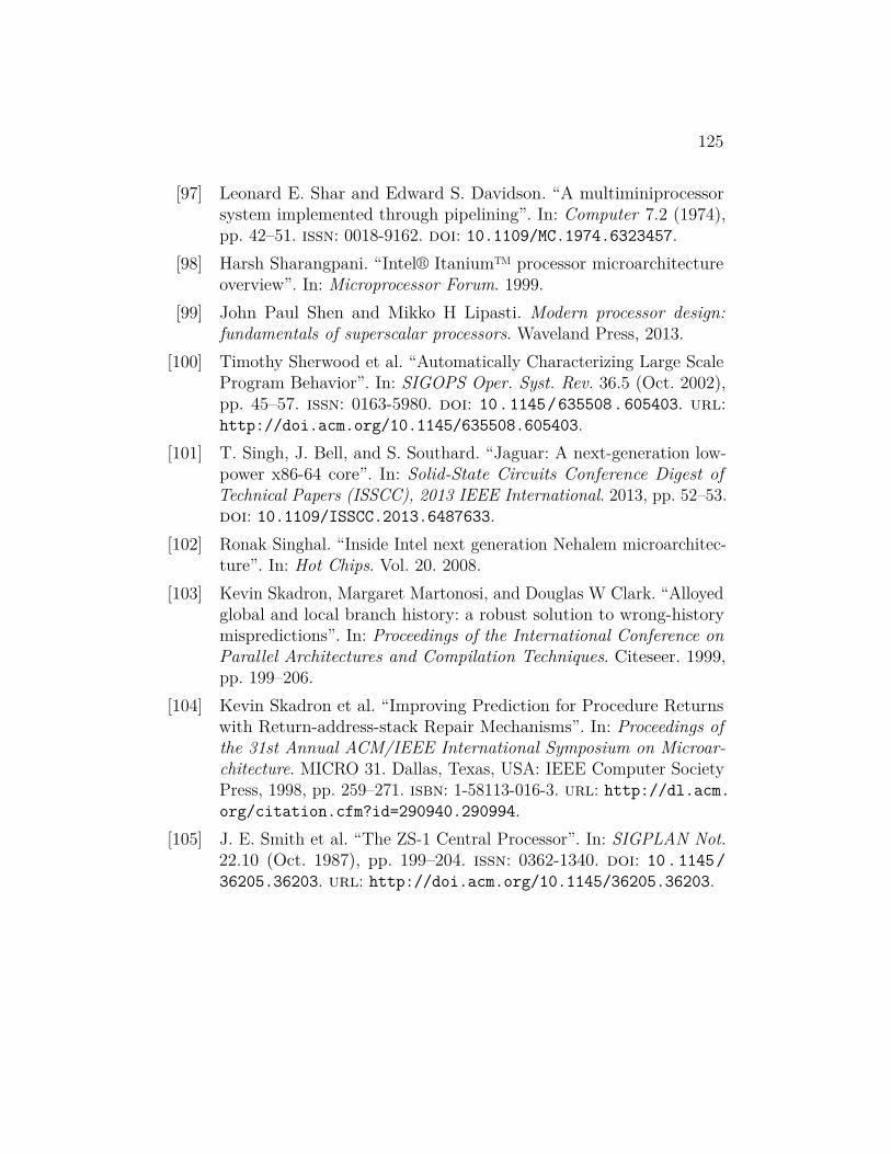
125
[97] Leonard E. Shar and Edward S. Davidson. “A multiminiprocessorsystem implemented through pipelining”. In: Computer 7.2 (1974),pp. 42–51. issn: 0018-9162. doi: 10.1109/MC.1974.6323457.
[98] Harsh Sharangpani. “Intel® Itanium™ processor microarchitectureoverview”. In: Microprocessor Forum. 1999.
[99] John Paul Shen and Mikko H Lipasti. Modern processor design:fundamentals of superscalar processors. Waveland Press, 2013.
[100] Timothy Sherwood et al. “Automatically Characterizing Large ScaleProgram Behavior”. In: SIGOPS Oper. Syst. Rev. 36.5 (Oct. 2002),pp. 45–57. issn: 0163-5980. doi: 10.1145/635508.605403. url:http://doi.acm.org/10.1145/635508.605403.
[101] T. Singh, J. Bell, and S. Southard. “Jaguar: A next-generation low-power x86-64 core”. In: Solid-State Circuits Conference Digest ofTechnical Papers (ISSCC), 2013 IEEE International. 2013, pp. 52–53.doi: 10.1109/ISSCC.2013.6487633.
[102] Ronak Singhal. “Inside Intel next generation Nehalem microarchitec-ture”. In: Hot Chips. Vol. 20. 2008.
[103] Kevin Skadron, Margaret Martonosi, and Douglas W Clark. “Alloyedglobal and local branch history: a robust solution to wrong-historymispredictions”. In: Proceedings of the International Conference onParallel Architectures and Compilation Techniques. Citeseer. 1999,pp. 199–206.
[104] Kevin Skadron et al. “Improving Prediction for Procedure Returnswith Return-address-stack Repair Mechanisms”. In: Proceedings ofthe 31st Annual ACM/IEEE International Symposium on Microar-chitecture. MICRO 31. Dallas, Texas, USA: IEEE Computer SocietyPress, 1998, pp. 259–271. isbn: 1-58113-016-3. url: http://dl.acm.org/citation.cfm?id=290940.290994.
[105] J. E. Smith et al. “The ZS-1 Central Processor”. In: SIGPLAN Not.22.10 (Oct. 1987), pp. 199–204. issn: 0362-1340. doi: 10.1145/36205.36203. url: http://doi.acm.org/10.1145/36205.36203.
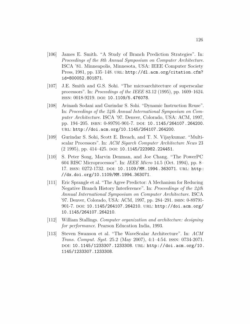
126
[106] James E. Smith. “A Study of Branch Prediction Strategies”. In:Proceedings of the 8th Annual Symposium on Computer Architecture.ISCA ’81. Minneapolis, Minnesota, USA: IEEE Computer SocietyPress, 1981, pp. 135–148. url: http://dl.acm.org/citation.cfm?id=800052.801871.
[107] J.E. Smith and G.S. Sohi. “The microarchitecture of superscalarprocessors”. In: Proceedings of the IEEE 83.12 (1995), pp. 1609–1624.issn: 0018-9219. doi: 10.1109/5.476078.
[108] Avinash Sodani and Gurindar S. Sohi. “Dynamic Instruction Reuse”.In: Proceedings of the 24th Annual International Symposium on Com-puter Architecture. ISCA ’97. Denver, Colorado, USA: ACM, 1997,pp. 194–205. isbn: 0-89791-901-7. doi: 10.1145/264107.264200.url: http://doi.acm.org/10.1145/264107.264200.
[109] Gurindar S. Sohi, Scott E. Breach, and T. N. Vijaykumar. “Multi-scalar Processors”. In: ACM Sigarch Computer Architecture News 23(2 1995), pp. 414–425. doi: 10.1145/223982.224451.
[110] S. Peter Song, Marvin Denman, and Joe Chang. “The PowerPC604 RISC Microprocessor”. In: IEEE Micro 14.5 (Oct. 1994), pp. 8–17. issn: 0272-1732. doi: 10.1109/MM.1994.363071. url: http://dx.doi.org/10.1109/MM.1994.363071.
[111] Eric Sprangle et al. “The Agree Predictor: A Mechanism for ReducingNegative Branch History Interference”. In: Proceedings of the 24thAnnual International Symposium on Computer Architecture. ISCA’97. Denver, Colorado, USA: ACM, 1997, pp. 284–291. isbn: 0-89791-901-7. doi: 10.1145/264107.264210. url: http://doi.acm.org/10.1145/264107.264210.
[112] William Stallings. Computer organization and architecture: designingfor performance. Pearson Education India, 1993.
[113] Steven Swanson et al. “The WaveScalar Architecture”. In: ACMTrans. Comput. Syst. 25.2 (May 2007), 4:1–4:54. issn: 0734-2071.doi: 10.1145/1233307.1233308. url: http://doi.acm.org/10.1145/1233307.1233308.
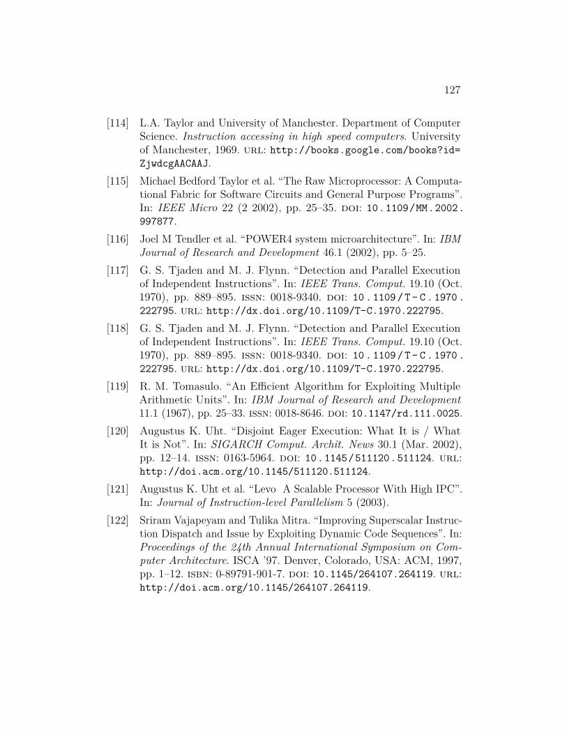
127
[114] L.A. Taylor and University of Manchester. Department of ComputerScience. Instruction accessing in high speed computers. Universityof Manchester, 1969. url: http://books.google.com/books?id=ZjwdcgAACAAJ.
[115] Michael Bedford Taylor et al. “The Raw Microprocessor: A Computa-tional Fabric for Software Circuits and General Purpose Programs”.In: IEEE Micro 22 (2 2002), pp. 25–35. doi: 10.1109/MM.2002.997877.
[116] Joel M Tendler et al. “POWER4 system microarchitecture”. In: IBMJournal of Research and Development 46.1 (2002), pp. 5–25.
[117] G. S. Tjaden and M. J. Flynn. “Detection and Parallel Executionof Independent Instructions”. In: IEEE Trans. Comput. 19.10 (Oct.1970), pp. 889–895. issn: 0018-9340. doi: 10 . 1109 / T - C . 1970 .222795. url: http://dx.doi.org/10.1109/T-C.1970.222795.
[118] G. S. Tjaden and M. J. Flynn. “Detection and Parallel Executionof Independent Instructions”. In: IEEE Trans. Comput. 19.10 (Oct.1970), pp. 889–895. issn: 0018-9340. doi: 10 . 1109 / T - C . 1970 .222795. url: http://dx.doi.org/10.1109/T-C.1970.222795.
[119] R. M. Tomasulo. “An Efficient Algorithm for Exploiting MultipleArithmetic Units”. In: IBM Journal of Research and Development11.1 (1967), pp. 25–33. issn: 0018-8646. doi: 10.1147/rd.111.0025.
[120] Augustus K. Uht. “Disjoint Eager Execution: What It is / WhatIt is Not”. In: SIGARCH Comput. Archit. News 30.1 (Mar. 2002),pp. 12–14. issn: 0163-5964. doi: 10.1145/511120.511124. url:http://doi.acm.org/10.1145/511120.511124.
[121] Augustus K. Uht et al. “Levo A Scalable Processor With High IPC”.In: Journal of Instruction-level Parallelism 5 (2003).
[122] Sriram Vajapeyam and Tulika Mitra. “Improving Superscalar Instruc-tion Dispatch and Issue by Exploiting Dynamic Code Sequences”. In:Proceedings of the 24th Annual International Symposium on Com-puter Architecture. ISCA ’97. Denver, Colorado, USA: ACM, 1997,pp. 1–12. isbn: 0-89791-901-7. doi: 10.1145/264107.264119. url:http://doi.acm.org/10.1145/264107.264119.
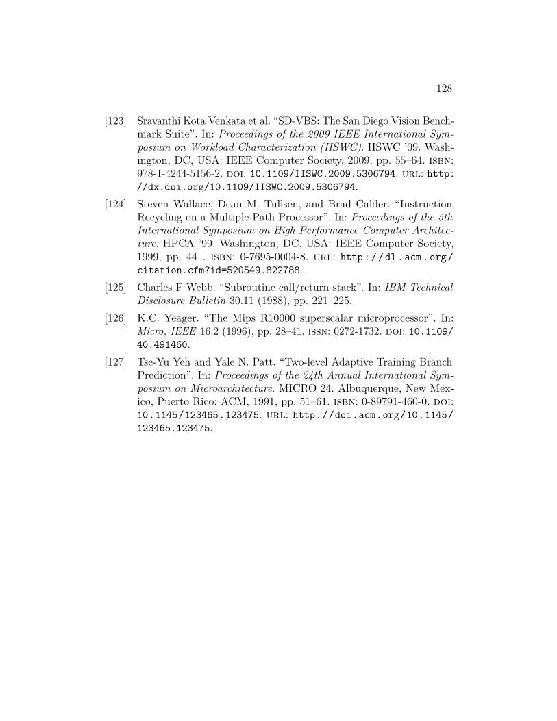
128
[123] Sravanthi Kota Venkata et al. “SD-VBS: The San Diego Vision Bench-mark Suite”. In: Proceedings of the 2009 IEEE International Sym-posium on Workload Characterization (IISWC). IISWC ’09. Wash-ington, DC, USA: IEEE Computer Society, 2009, pp. 55–64. isbn:978-1-4244-5156-2. doi: 10.1109/IISWC.2009.5306794. url: http://dx.doi.org/10.1109/IISWC.2009.5306794.
[124] Steven Wallace, Dean M. Tullsen, and Brad Calder. “InstructionRecycling on a Multiple-Path Processor”. In: Proceedings of the 5thInternational Symposium on High Performance Computer Architec-ture. HPCA ’99. Washington, DC, USA: IEEE Computer Society,1999, pp. 44–. isbn: 0-7695-0004-8. url: http://dl.acm.org/citation.cfm?id=520549.822788.
[125] Charles F Webb. “Subroutine call/return stack”. In: IBM TechnicalDisclosure Bulletin 30.11 (1988), pp. 221–225.
[126] K.C. Yeager. “The Mips R10000 superscalar microprocessor”. In:Micro, IEEE 16.2 (1996), pp. 28–41. issn: 0272-1732. doi: 10.1109/40.491460.
[127] Tse-Yu Yeh and Yale N. Patt. “Two-level Adaptive Training BranchPrediction”. In: Proceedings of the 24th Annual International Sym-posium on Microarchitecture. MICRO 24. Albuquerque, New Mex-ico, Puerto Rico: ACM, 1991, pp. 51–61. isbn: 0-89791-460-0. doi:10.1145/123465.123475. url: http://doi.acm.org/10.1145/123465.123475.