Express Introductory Training in ANSYS Fluent · PDF fileFluent will still use the default material in the cell zones. Since you cannot delete a material that is in use, this step

© 2012 ANSYS, Inc. September 19, 2013 1 Release 14.5

PRACE Autumn School 2013 - Industry Oriented HPC Simulations, September 21-27,

University of Ljubljana, Faculty of Mechanical Engineering, Ljubljana, Slovenia

Express Introductory Training in ANSYS Fluent

Workshop 02

Using the Discrete Phase Model (DPM)

Dimitrios Sofialidis

Technical Manager, SimTec Ltd.

Mechanical Engineer, PhD


14. 0 Release

Introduction to ANSYS Fluent

Workshop 02 Using the Discrete Phase Model (DPM)


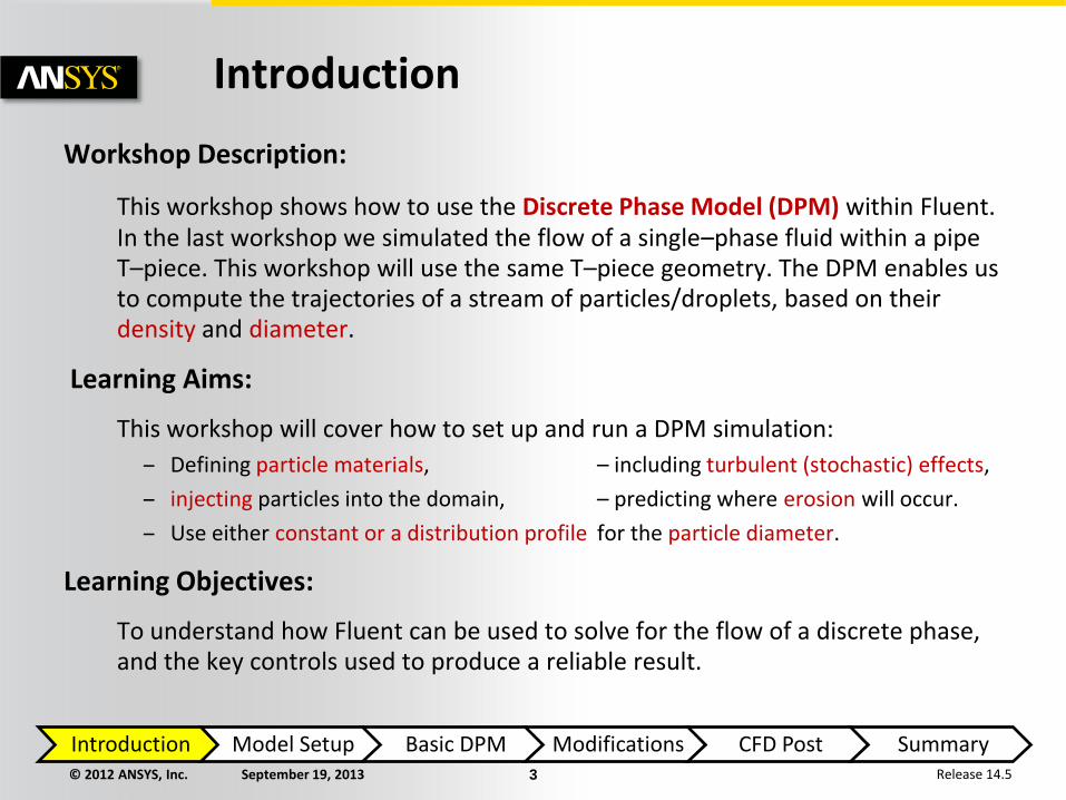
Workshop Description:

This workshop shows how to use the Discrete Phase Model (DPM) within Fluent. In the last workshop we simulated the flow of a single–phase fluid within a pipe T–piece. This workshop will use the same T–piece geometry. The DPM enables us to compute the trajectories of a stream of particles/droplets, based on their density and diameter.

Learning Aims:

This workshop will cover how to set up and run a DPM simulation:

– Defining particle materials, – including turbulent (stochastic) effects,

– injecting particles into the domain, – predicting where erosion will occur.

– Use either constant or a distribution profile for the particle diameter.

Learning Objectives:

To understand how Fluent can be used to solve for the flow of a discrete phase, and the key controls used to produce a reliable result.

I Introduction

Introduction Model Setup Basic DPM Modifications CFD Post Summary


Simulation to be performed

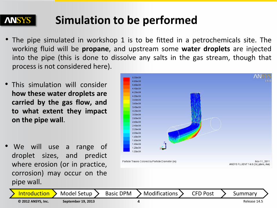
• The pipe simulated in workshop 1 is to be fitted in a petrochemicals site. The working fluid will be propane, and upstream some water droplets are injected into the pipe (this is done to dissolve any salts in the gas stream, though that process is not considered here).

• This simulation will consider how these water droplets are carried by the gas flow, and to what extent they impact on the pipe wall.

• We will use a range of droplet sizes, and predict where erosion (or in practice, corrosion) may occur on the pipe wall.



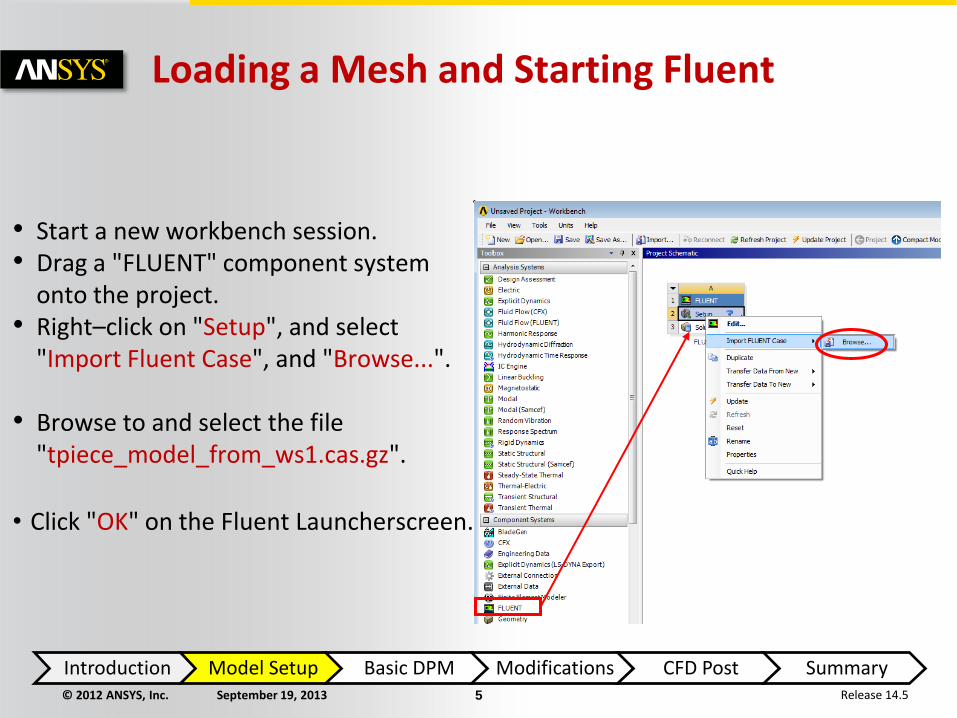
• Start a new workbench session. • Drag a "FLUENT" component system onto the project. • Right–click on "Setup", and select "Import Fluent Case", and "Browse...".

• Browse to and select the file "tpiece_model_from_ws1.cas.gz".

• Click "OK" on the Fluent Launcherscreen.

Loading a Mesh and Starting Fluent



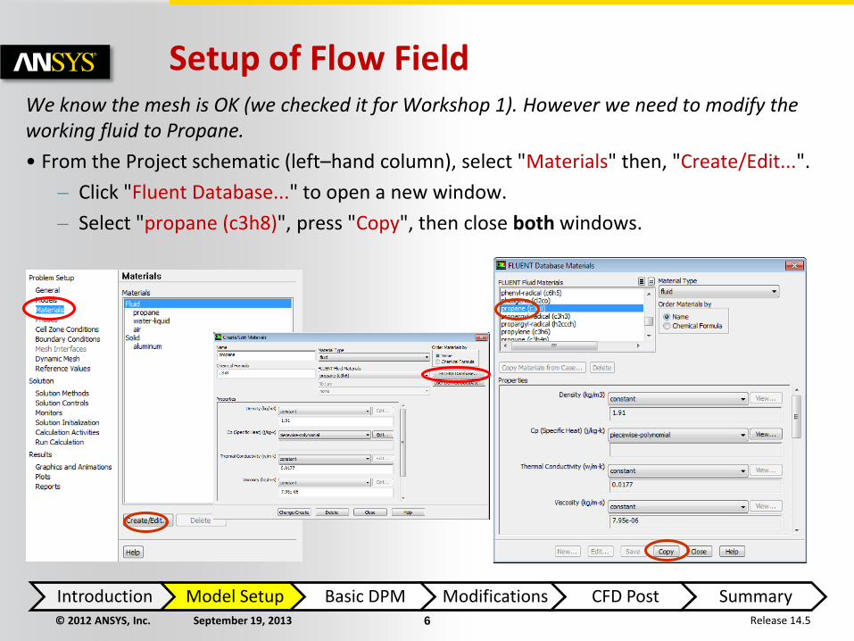
We know the mesh is OK (we checked it for Workshop 1). However we need to modify the working fluid to Propane.

• From the Project schematic (left–hand column), select "Materials" then, "Create/Edit...".

– Click "Fluent Database..." to open a new window.

– Select "propane (c3h8)", press "Copy", then close both windows.

Setup of Flow Field



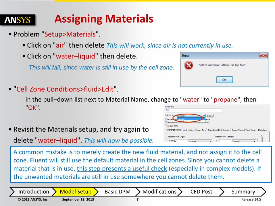
• Problem "Setup>Materials".

• Click on "air" then delete This will work, since air is not currently in use.

• Click on "water–liquid" then delete.

This will fail, since water is still in use by the cell zone.

• "Cell Zone Conditions>fluid>Edit".

– In the pull–down list next to Material Name, change to "water" to "propane", then "OK".

• Revisit the Materials setup, and try again to

delete "water–liquid". This will now be possible.

Assigning Materials

A common mistake is to merely create the new fluid material, and not assign it to the cell zone. Fluent will still use the default material in the cell zones. Since you cannot delete a material that is in use, this step presents a useful check (especially in complex models). If the unwanted materials are still in use somewhere you cannot delete them.



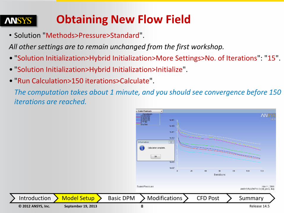
Obtaining New Flow Field • Solution "Methods>Pressure>Standard".

All other settings are to remain unchanged from the first workshop.

• "Solution Initialization>Hybrid Initialization>More Settings>No. of Iterations": "15".

• "Solution Initialization>Hybrid Initialization>Initialize".

• "Run Calculation>150 iterations>Calculate".

The computation takes about 1 minute, and you should see convergence before 150 iterations are reached.



Basic DPM Setup [1] • From the project schematic (left–hand toolbar), select "Models", "Discrete Phase", then

"Edit".

• On the "Discrete Phase Model" pane, select "Injections".

• In the "Injections" panel, select "Create".

This will open up the "Injections" panel.



Basic DPM Setup [2] • Setup a new injection as follows: • Set injection type to "surface".

• Pick surface "inlet–z".

• Keep default material "anthracite".

• Keep default diameter "uniform".

• "X–Velocity" "0 [m/s]"

• "Y–Velocity" "0 [m/s]"

• "Z–Velocity" "–1 [m/s]"

• "Diameter" "1e–04 [m]"

• "Temperature" "90 (c)"

• "Flow Rate" "1 [kg/s]"

• Tick "Scale Flow Rate by Face Area".

• Select "OK" to close this window.

• "Close" the "Injections" Window.

• "OK" on the "Discrete Phase Model"

window.

Only when we have set up a DPM injection can we get access to define the particle material. We will change this on the next slide.

There are many ways to introduce DPM particles (parcels). Although here we use a boundary surface present in the geometry, we could choose to inject at XYZ point co–ordinates anywhere within the model.



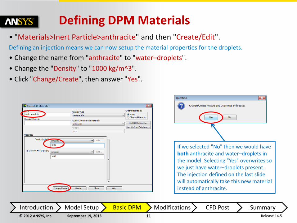
Defining DPM Materials • "Materials>Inert Particle>anthracite" and then "Create/Edit". Defining an injection means we can now setup the material properties for the droplets.

• Change the name from "anthracite" to "water–droplets".

• Change the "Density" to "1000 kg/m^3".

• Click "Change/Create", then answer "Yes".

If we selected "No" then we would have both anthracite and water–droplets in the model. Selecting "Yes" overwrites so we just have water–droplets present. The injection defined on the last slide will automatically take this new material instead of anthracite.



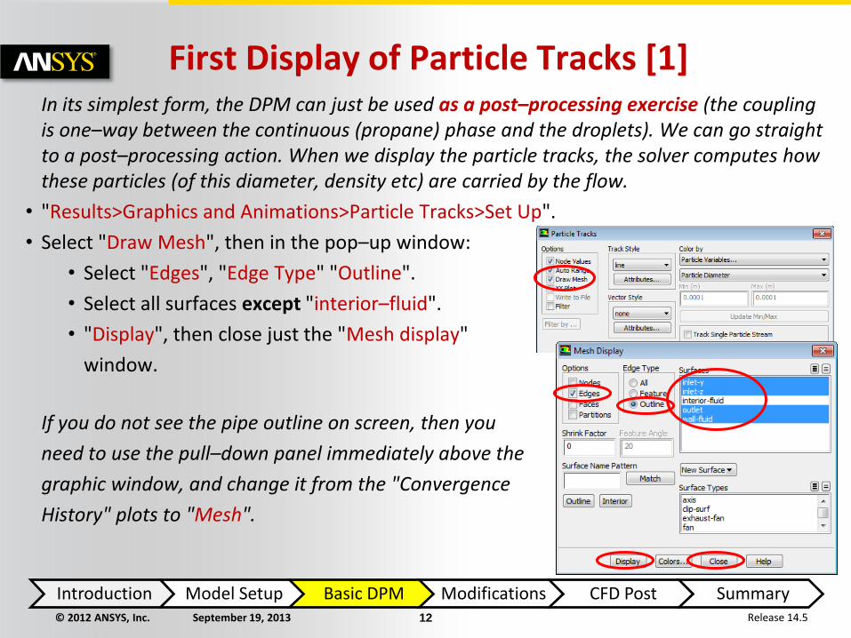
First Display of Particle Tracks [1] In its simplest form, the DPM can just be used as a post–processing exercise (the coupling

is one–way between the continuous (propane) phase and the droplets). We can go straight to a post–processing action. When we display the particle tracks, the solver computes how these particles (of this diameter, density etc) are carried by the flow.

• "Results>Graphics and Animations>Particle Tracks>Set Up".

• Select "Draw Mesh", then in the pop–up window:

• Select "Edges", "Edge Type" "Outline".

• Select all surfaces except "interior–fluid".

• "Display", then close just the "Mesh display"

window.

If you do not see the pipe outline on screen, then you

need to use the pull–down panel immediately above the

graphic window, and change it from the "Convergence

History" plots to "Mesh".



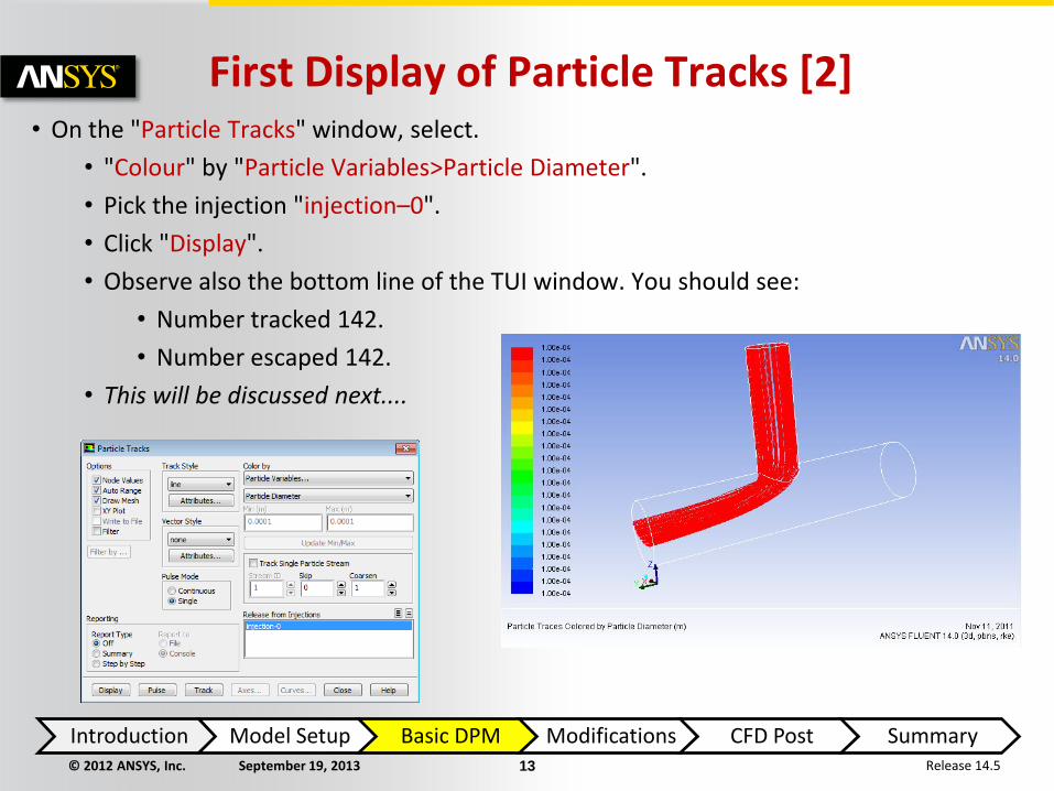
First Display of Particle Tracks [2] • On the "Particle Tracks" window, select.

• "Colour" by "Particle Variables>Particle Diameter".

• Pick the injection "injection–0".

• Click "Display".

• Observe also the bottom line of the TUI window. You should see:

• Number tracked 142.

• Number escaped 142.

• This will be discussed next....



Discussion on DPM [1]

In this example, Fluent has released one droplet from each face on the "outlet" boundary. There are 142 faces in the mesh here, hence 142 trajectories.

• Each droplet has a diameter of 1x10–4 [m], and a density of 1000 [kg/m3]. • Therefore each droplet has a mass of 5.2x10–10 [kg] (4/3 rpr3). • It is assumed that any droplet released from the same location with the same conditions

will follow the same trajectory. • Our mass flow rate is 1 [kg/s]. • So each of the 142 droplet trajectories computed is used to represent 1.3x106 actual

[droplets/s] 1/(5.2x10–10x142).

• The droplet (or particle) progresses through the domain through a large number of small steps. At each step, the solver computes the force balance acting on a single droplet (diameter 1x10–4 [m]) – hence considering the drag with the surrounding fluid, droplet inertia, and if applicable gravity. The mass transported is that of all the droplets in that stream (1.3x106 [droplets/s]).



Discussion on DPM [2]

• The coupling of the droplet (DPM) motion with that of the continuous phase can either be one–way or two–way coupled. The present example is one–way coupled. By this we mean that the fluid affects the momentum/energy of the DPM. But the surrounding fluid flow (propane) remains unaffected by the momentum/energy

exchange with the DPM. For this reason, we can use the DPM as a post–processing exercise, and quickly compute

the particle solution. • If required, two–way coupled behaviour can be enabled by setting "Interaction with Continuous

Phase" on the DPM set–up panel. One would then need to perform additional iterations of the (propane) flow field to

convergence. It is not usually necessary to solve the DPM at every flow iteration. Typically the DPM field

needs updating every 5–10 flow iterations.



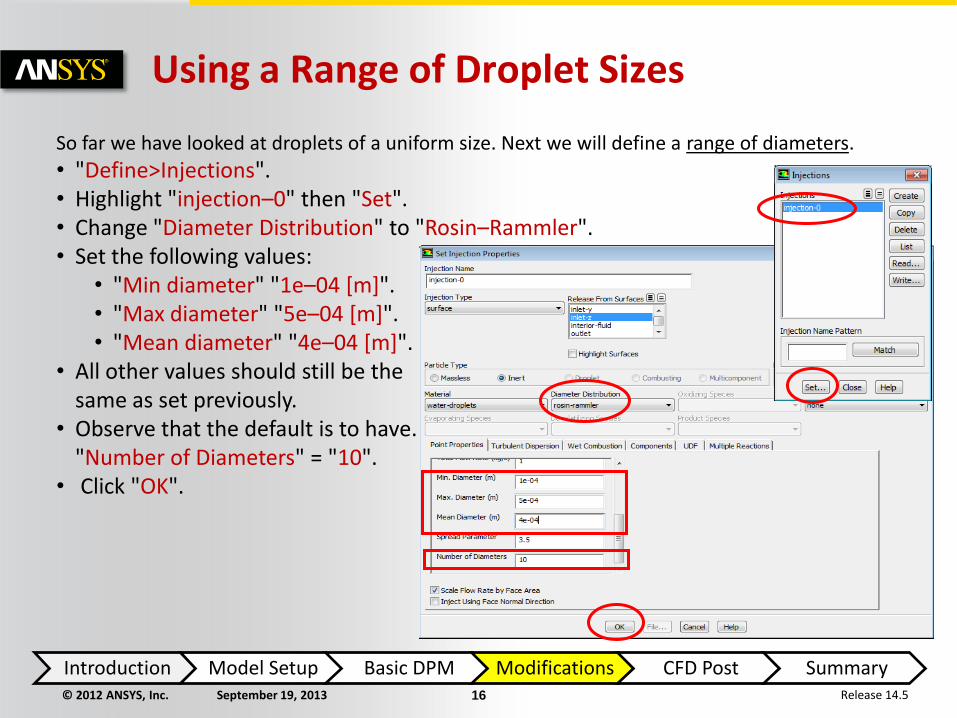
Using a Range of Droplet Sizes

So far we have looked at droplets of a uniform size. Next we will define a range of diameters.

• "Define>Injections". • Highlight "injection–0" then "Set". • Change "Diameter Distribution" to "Rosin–Rammler". • Set the following values:

• "Min diameter" "1e–04 [m]". • "Max diameter" "5e–04 [m]". • "Mean diameter" "4e–04 [m]".

• All other values should still be the same as set previously.

• Observe that the default is to have. "Number of Diameters" = "10". • Click "OK".



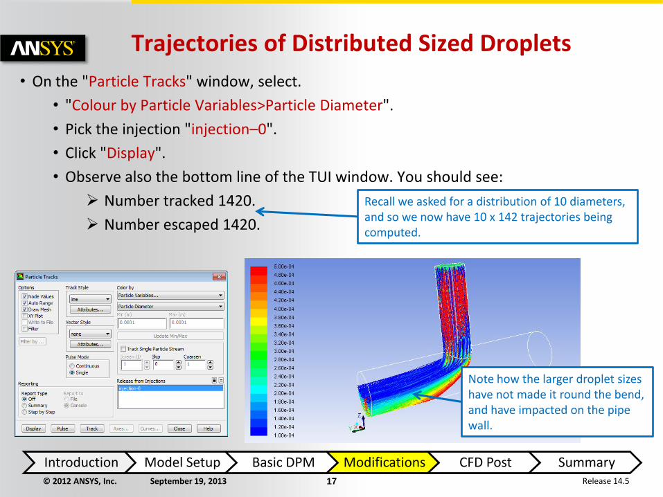
Trajectories of Distributed Sized Droplets

• On the "Particle Tracks" window, select.

• "Colour by Particle Variables>Particle Diameter".




Number tracked 1420.

Number escaped 1420.

Note how the larger droplet sizes have not made it round the bend, and have impacted on the pipe wall.

Recall we asked for a distribution of 10 diameters, and so we now have 10 x 142 trajectories being computed.



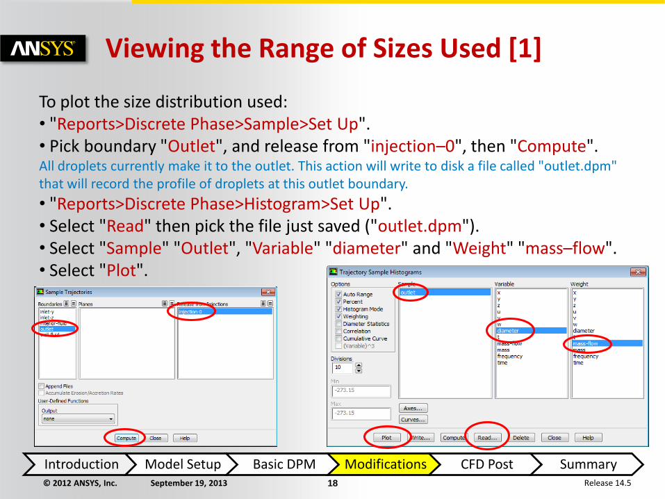
Viewing the Range of Sizes Used [1]

To plot the size distribution used: • "Reports>Discrete Phase>Sample>Set Up". • Pick boundary "Outlet", and release from "injection–0", then "Compute". All droplets currently make it to the outlet. This action will write to disk a file called "outlet.dpm" that will record the profile of droplets at this outlet boundary.

• "Reports>Discrete Phase>Histogram>Set Up". • Select "Read" then pick the file just saved ("outlet.dpm"). • Select "Sample" "Outlet", "Variable" "diameter" and "Weight" "mass–flow". • Select "Plot".



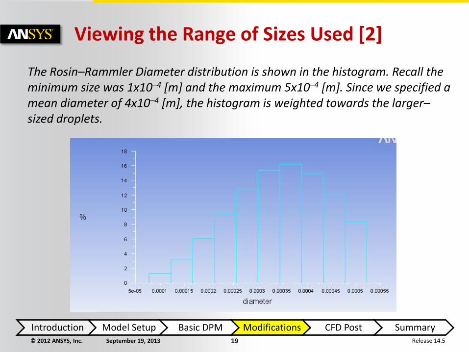
Viewing the Range of Sizes Used [2]

The Rosin–Rammler Diameter distribution is shown in the histogram. Recall the minimum size was 1x10–4 [m] and the maximum 5x10–4 [m]. Since we specified a mean diameter of 4x10–4 [m], the histogram is weighted towards the larger–sized droplets.



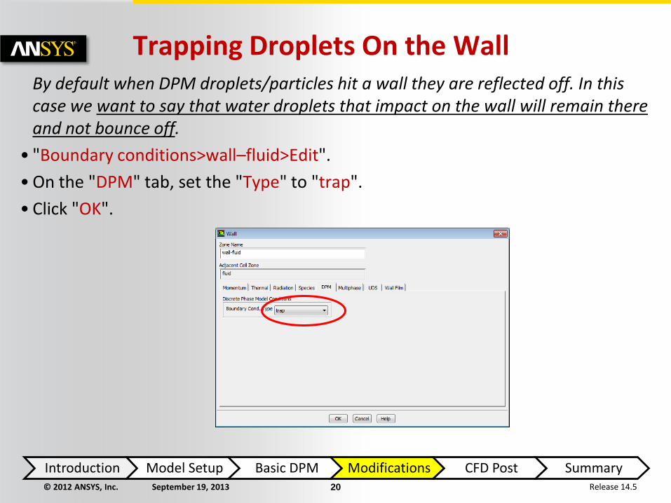
Trapping Droplets On the Wall By default when DPM droplets/particles hit a wall they are reflected off. In this

case we want to say that water droplets that impact on the wall will remain there and not bounce off.

• "Boundary conditions>wall–fluid>Edit".

• On the "DPM" tab, set the "Type" to "trap".

• Click "OK".



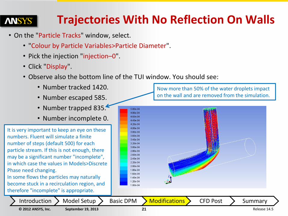
Trajectories With No Reflection On Walls • On the "Particle Tracks" window, select.







• Number trapped 835.

• Number incomplete 0.

Now more than 50% of the water droplets impact on the wall and are removed from the simulation.

It is very important to keep an eye on these numbers. Fluent will simulate a finite number of steps (default 500) for each particle stream. If this is not enough, there may be a significant number "incomplete", in which case the values in Models>Discrete Phase need changing. In some flows the particles may naturally become stuck in a recirculation region, and therefore "incomplete" is appropriate.



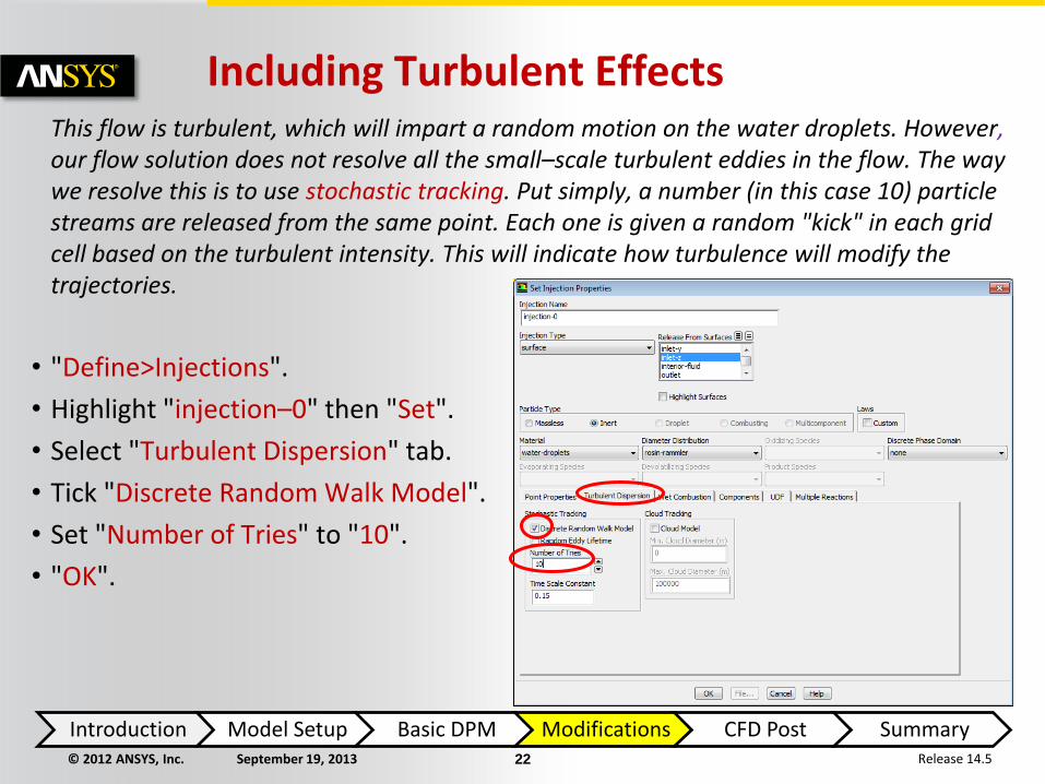
Including Turbulent Effects This flow is turbulent, which will impart a random motion on the water droplets. However,

our flow solution does not resolve all the small–scale turbulent eddies in the flow. The way we resolve this is to use stochastic tracking. Put simply, a number (in this case 10) particle streams are released from the same point. Each one is given a random "kick" in each grid cell based on the turbulent intensity. This will indicate how turbulence will modify the trajectories.

• "Define>Injections".

• Highlight "injection–0" then "Set".

• Select "Turbulent Dispersion" tab.

• Tick "Discrete Random Walk Model".

• Set "Number of Tries" to "10".

• "OK".



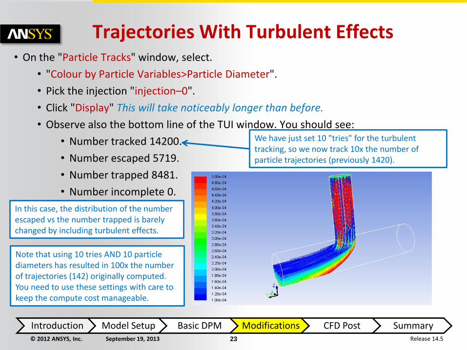
Trajectories With Turbulent Effects • On the "Particle Tracks" window, select.



• Click "Display" This will take noticeably longer than before.




• Number trapped 8481.

• Number incomplete 0.

We have just set 10 "tries" for the turbulent tracking, so we now track 10x the number of particle trajectories (previously 1420).

In this case, the distribution of the number escaped vs the number trapped is barely changed by including turbulent effects.

Note that using 10 tries AND 10 particle diameters has resulted in 100x the number of trajectories (142) originally computed. You need to use these settings with care to keep the compute cost manageable.



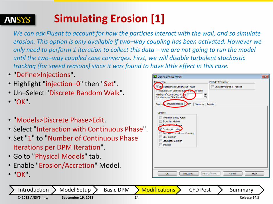
We can ask Fluent to account for how the particles interact with the wall, and so simulate erosion. This option is only available if two–way coupling has been activated. However we only need to perform 1 iteration to collect this data – we are not going to run the model until the two–way coupled case converges. First, we will disable turbulent stochastic tracking (for speed reasons) since it was found to have little effect in this case.

• "Define>Injections". • Highlight "injection–0" then "Set". • Un–Select "Discrete Random Walk". • "OK".

• "Models>Discrete Phase>Edit. • Select "Interaction with Continuous Phase". • Set "1" to "Number of Continuous Phase Iterations per DPM Iteration". • Go to "Physical Models" tab. • Enable "Erosion/Accretion" Model. • "OK".

Simulating Erosion [1]



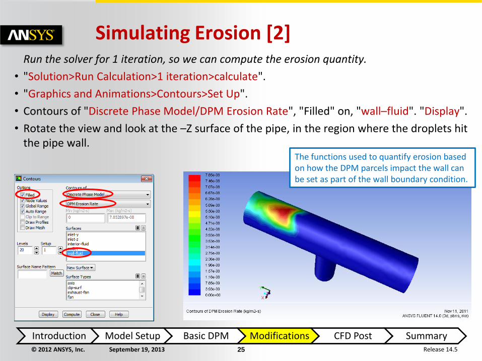
Run the solver for 1 iteration, so we can compute the erosion quantity.

• "Solution>Run Calculation>1 iteration>calculate".

• "Graphics and Animations>Contours>Set Up".

• Contours of "Discrete Phase Model/DPM Erosion Rate", "Filled" on, "wall–fluid". "Display".

• Rotate the view and look at the –Z surface of the pipe, in the region where the droplets hit the pipe wall.

Simulating Erosion [2]

The functions used to quantify erosion based on how the DPM parcels impact the wall can be set as part of the wall boundary condition.



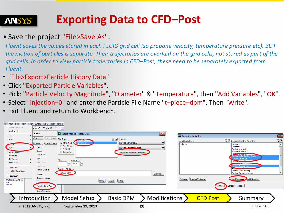
Exporting Data to CFD–Post

• Save the project "File>Save As". Fluent saves the values stored in each FLUID grid cell (so propane velocity, temperature pressure etc). BUT the motion of particles is separate. Their trajectories are overlaid on the grid cells, not stored as part of the grid cells. In order to view particle trajectories in CFD–Post, these need to be separately exported from Fluent.

• "File>Export>Particle History Data". • Click "Exported Particle Variables". • Pick: "Particle Velocity Magnitude", "Diameter" & "Temperature", then "Add Variables", "OK". • Select "injection–0" and enter the Particle File Name "t–piece–dpm". Then "Write". • Exit Fluent and return to Workbench.



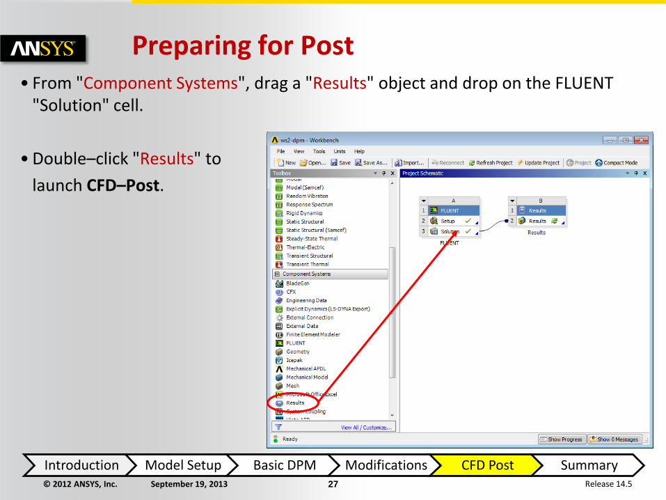
Preparing for Post • From "Component Systems", drag a "Results" object and drop on the FLUENT

"Solution" cell.

• Double–click "Results" to

launch CFD–Post.



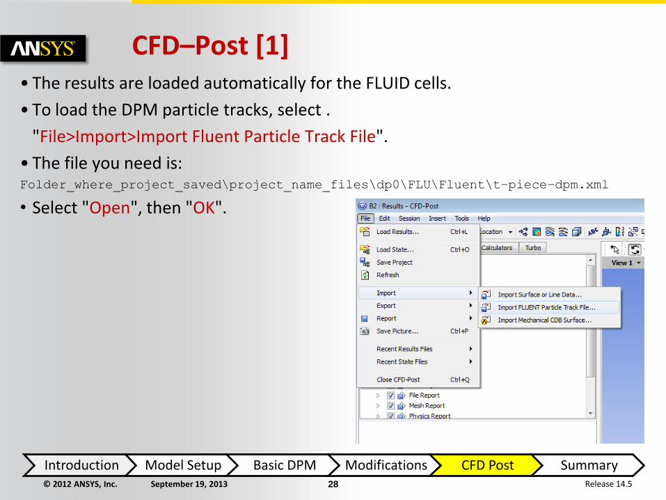
CFD–Post [1] • The results are loaded automatically for the FLUID cells.

• To load the DPM particle tracks, select .

"File>Import>Import Fluent Particle Track File".

• The file you need is: Folder_where_project_saved\project_name_files\dp0\FLU\Fluent\t–piece–dpm.xml

• Select "Open", then "OK".



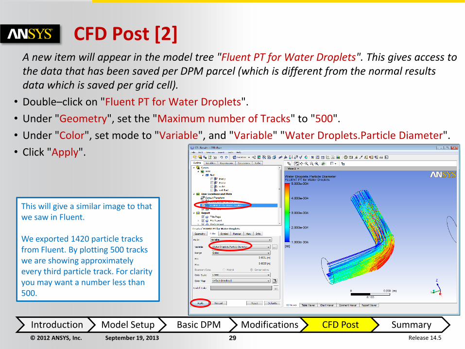
CFD Post [2] A new item will appear in the model tree "Fluent PT for Water Droplets". This gives access to

the data that has been saved per DPM parcel (which is different from the normal results data which is saved per grid cell).

• Double–click on "Fluent PT for Water Droplets".

• Under "Geometry", set the "Maximum number of Tracks" to "500".

• Under "Color", set mode to "Variable", and "Variable" "Water Droplets.Particle Diameter".

• Click "Apply".

This will give a similar image to that we saw in Fluent. We exported 1420 particle tracks from Fluent. By plotting 500 tracks we are showing approximately every third particle track. For clarity you may want a number less than 500.



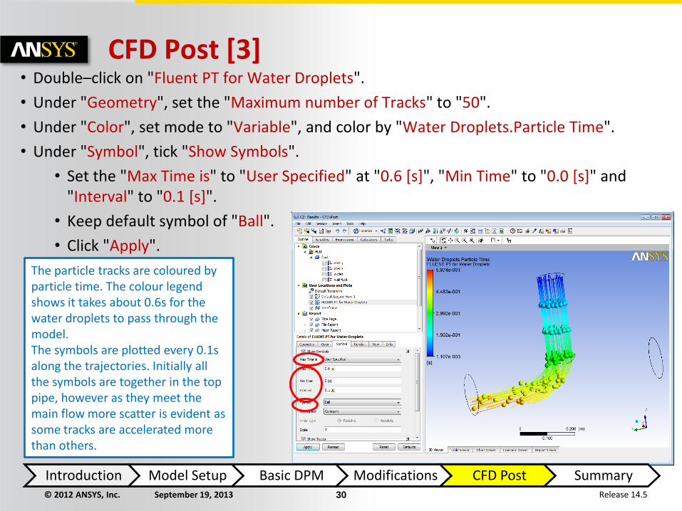
CFD Post [3] • Double–click on "Fluent PT for Water Droplets".

• Under "Geometry", set the "Maximum number of Tracks" to "50".

• Under "Color", set mode to "Variable", and color by "Water Droplets.Particle Time".

• Under "Symbol", tick "Show Symbols".

• Set the "Max Time is" to "User Specified" at "0.6 [s]", "Min Time" to "0.0 [s]" and "Interval" to "0.1 [s]".

• Keep default symbol of "Ball".

• Click "Apply".

The particle tracks are coloured by particle time. The colour legend shows it takes about 0.6s for the water droplets to pass through the model. The symbols are plotted every 0.1s along the trajectories. Initially all the symbols are together in the top pipe, however as they meet the main flow more scatter is evident as some tracks are accelerated more than others.



Wrap–Up [1]

This workshop has shown how Fluent can be used to simulate the motion of fluid droplets (or solid particles) that are carried along by the fluid.

• Regular CFD simulations are performed in an "Eulerian" reference frame. The mesh remains fixed, and material flows through the grid (aka mesh) cells. When simulating particle tracks, these move in a "Lagrangian" reference frame. The particles/droplets each have their own X,Y,Z co–ordinates and their properties are stored separately from the grid cell (normal data) file quantities.

• The user sets the diameter and density of the particles to be simulated. The trajectory through the domain is computed over a large number of small steps. At each step their relaxation time can be computed (from knowing their inertia, and the sum of the forces acting on each droplet/particle).

• Here we have performed several different particle–trajectory simulations to investigate:

• The effect of droplet diameter. • The effect of droplets being "trapped" as they hit a wall. • The effects of turbulence (random walk model/stochastic tracking).



Wrap–Up [2]

Using the discrete–phase model, there are several other enhancements to this basic setup that we could simulate:

• Coupling the DPM motion to that of the continuous phase (so that the surrounding propane has its own momentum/temperature modified by the presence of the droplets).

• Simulating multi–component particles: Sample application: An industrial spray drier. Solid particles are introduced

which have a moisture content. Thermal energy is taken from the surrounding fluid, the moisture is removed from the particles making them lighter. Simultaneously this water is added in vapour phase to the continuous phase.

• Simulating reacting particles: Sample application: A coal burner for a power station. The volatile components of the coal particle evaporate, and react with the surrounding air generating

heat.


Documents

Express Introductory Training in ANSYS Fluent · PDF fileFluent will still use the default material in the cell zones. Since you cannot delete a material that is in use, this step