Embed Size (px)
Citation preview
Exports and Growth Shocks:
How Export Growth Depends on Economic Development
Jesse Mora
(Occidental College)
Michael Olabisi∗
(Michigan State University)
Abstract
We offer a new decomposition approach that explains long-run export
growth, and how export growth varies by economic development. The
approach relies on a heterogeneous-firm model that defines the key mar-
gins for export growth: comparative advantage shocks, product growth
shocks, country-level growth shocks, global growth shocks, and growth
in destinations reached. From the model, we develop predictions that
link export growth at the country-product level to these margins, and
that show how the effect of each margin of trade depends on economic
development. In testing the predictions, we show systematic differences
between countries at different stages of economic development. Specif-
ically, we show that the product shock margin is a stronger driver of
exports for high-income countries, but is less so for middle-income and
low-income countries. The country shock margin is more important for
explaining export growth in middle-income countries, compared to other
country-groups. Global shock margin appear to benefit developed coun-
tries more, though those results are not as robust. Finally, having more
destinations is the most notable driver of the observed export growth in
our analysis. The findings hold up to several robustness checks.
DATA AVAILABILITY STATEMENT
The data that support the findings of this study are available from the corre-sponding author upon reasonable request.
∗Author contacts: [email protected]; [email protected] We are thankful to Renee Bowen, par-ticipants at the San Francisco Western Economic Association International conference, and AlanSpearot for insightful comments. All errors are our own.
I Introduction
The contours of global trade are changing, with developing countries’ share of global
exports surging from 21.4% in 1995 to 42% in 2015. Can the surge of the past
two decades offer export growth lessons for the years to come? Aggregate exports
increased by a factor of 3.4 between 1995 and 2015, but the increase was by a
factor of 2.3 for high-income countries, a factor of 6 for middle income countries,
and a factor of 7.5 for low-income countries. In that period, changing tastes and
technology drove exports of cassette tapes (HS 852421) from more than $540 million
in 1995 to zero in 2015, just as exports of computers (HS 847120) increased almost
tenfold, from $15 billion to $146 billion. Countries like Vietnam saw their exports
increase by a factor of 33 in the two-decade period, while Gambia witnessed a decrease
from $185 to $120 million. Given that GDP growth for most developing economies
is tied to export growth, and with trade as a larger share of GDP for low-income
countries, it is important to understand the internal or external factors driving export
growth, and, how different countries benefit differently from growth shocks that may
affect products and countries differently. The changes in global trade motivate us to
ask whether studying how exports increased in economies like Vietnam, China and
Colombia can be useful for economies like Gambia and Guatemala, where economic
growth still remains a pressing challenge.1
To explain export growth in this period, and how it differed for countries at dif-
ferent levels of economic development, we offer a novel approach to export growth
decomposition. The decomposition is derived from a heterogeneous-firm model that
follows the productivity and aggregation assumptions in Spearot (2016), while asso-
ciating the parameters of the assumed Pareto distribution of firm productivity in a
country with its level of economic development, as in Mora and Olabisi (2020). Rec-
ognizing that firm-size distributions vary with economic development, is necessary to
show that countries respond differently to economic shocks and export opportunities.
In the model, country-level exports will respond to one or more of five growth
drivers (or shocks): [1] demand changes for specific products, exogenous to any
specific country, usually from changing consumer tastes or technology, as in the
motivating example of cassette tapes, [2] country-level shocks that drive demand
1The scale and scope of export growth in developing economies is a notable component of theextensive literature on trade and economic growth (e.g., Zymek, 2015; Hanson, 2012; Feenstra andWei, 2010). Papers in this vein have emphasized a range of options for developing economies thatinclude complementary government policies, trade openness and export product diversification (e.g.,Chang, Kaltani, and Loayza, 2009; Harrison, 1996; Ventura, 1997)
1
for all products in a national export portfolio, usually due to exchange rates, trade
policies, or other advantages that affect all exports for a given country, [3] changes
to comparative advantage for a specific set of products in a country, making them
more attractive to consumers abroad, [4] broad-based export growth in trade-able
products for all countries as real incomes grow globally, with connections between
markets becoming easier, and [5] changes to the number of export destinations for
a country. We call the first four growth margins, product shocks, country shocks,
comparative advantage changes, and global shocks. By this definition, a country’s
exports will grow because, its export portfolio has the “right” products, it uses the
right policies to promote exports of all items, it gains the advantage in exporting for
specific items, it shares in the broad pattern of global trade expansion, or it increases
the number of export destinations. We use this decomposition to explain the export
growth of 183 economies.2
The model addresses a gap between policy and the economic literature. We an-
swer the question, “how do exports grow?” based on items policy-makers understand
– like which products are exported, the number of destinations served by each prod-
uct, and secular demand growth across exported goods. In the context of a trade and
development strategy, the framework matches the broad questions before the typi-
cal policymaker. The drivers of trade growth in the framework are product-specific
factors – which fits policy questions about which products to export or to export
next; country-specific factors and secular global growth shocks – in response to pol-
icy questions about how much domestic policy matters, or what policies to emulate
from other economies; comparative advantage – to fit policy concerns about enabling
specific sectors or products; and, finally, the number of destinations reached – which
matches a broad of set of policy initiatives on expanding market access.
The framework – our primary contribution, is flexible, yet tractable. It points to
where policy at the national level may or may not help to drive development through
export growth. Without identifying specific policies, it also helps to identify how past
export growth relative to other countries is attributable to national policies, global
trends, and sector-specific advantages for each country. Policy makers may want
to know: Which is more important – what you export, or how many destinations
you reach with what you export? Developing countries may also be interested in
knowing how differences related to economic development change the prospects for
export growth. The framework proposed in this paper is geared to address these
2As outlined above, we use the term growth shocks throughout the paper to mean all factors thatprompt a (positive or negative) growth in exports, not necessarily sudden or disruptive changes.
2
questions.
Model predictions: The theoretical model yields three key propositions : [1] any
of the four growth shocks (excluding destination count growth) will lead to propor-
tionally more exports for the least-developed countries, relative to high- and middle-
income countries; [2] growth in destination numbers, all else equal, will leads to a
similar increase in export values across country groups, and [3] country shocks play
a greater role than product shocks in explaining export growth. The predictions
digress notably from the usual concerns about productivity, and fixed or variable
trade costs that dominate published papers.
The sum of our effort is a new look at how trade grows, using a framework that can
help tailor policies to countries, given their product mix and their stage of economic
development. The arguments that what you export matters (Hausmann, Hwang,
and Rodrik, 2007; Hidalgo, Klinger, Barabasi, and Hausmann, 2007), and where
you export to matters (Brambilla, Lederman, and Porto, 2012; Baliamoune-Lutz,
2011; Bastos and Silva, 2010), can be measured side-by-side in our framework, as
a tool for guiding how growth priorities are set. Our work also helps to measure
the relative importance of the export growth options documented in earlier work –
specializing or diversifying products (Koren and Tenreyro, 2013; Besedes and Prusa,
2011; Hummels and Klenow, 2005) and diversifying destinations (Newfarmer, Shaw,
and Walkenhorst, 2009; Rose, 2007).
Our research question is closely related to the growing body of work on the mar-
gins of export growth. Papers in this literature explain growth in terms of product
variety (e.g., Hummels and Klenow, 2005; Besedes and Prusa, 2011; Cadot, Carrere,
and Strauss-Kahn, 2011), country-level and destination effects (Eaton, Kortum, and
Kramarz, 2011; Di Giovanni and Levchenko, 2012), and changes at the firm-level or
other combinations (e.g., Chaney, 2008; Eaton, Eslava, Kugler, and Tybout, 2007;
Amiti and Freund, 2010). While work in this area has largely emphasized high-
income and middle-income countries, we focus on countries with the greatest room
to grow economically, and to potentially benefit from a new perspective on the rele-
vant margins for export growth. The decomposition approach proposed in this paper
differs notably from earlier works that emphasize the intensive vs. extensive margins
(e.g., Mora and Olabisi, 2020; Besedes and Prusa, 2011; Schott, 2008), or studies that
emphasize factor inputs and productivity in explaining export growth (e.g., Egger
and Prusa, 2016; Egger and Nigai, 2016, 2015).
The export growth decomposition exercise uses the Base pour l’Analyse du Com-
3
merce International (BACI) dataset (Gaulier and Zignago, 2010). The dataset in-
cludes 21 years of exports (1995-2015), for more than 200 countries, at the detailed
HS 6-digit product level. The roughly 20 million observations in the collapsed version
of the data we use, represent unique exporter-product-year combinations that define
both the patterns and the scale of trade at highly dis-aggregated levels. The data,
and aggregates created from the data, allow us to observe the margins of export
growth in great detail.
Findings: As predicted by the model, export growth is driven by growth in the
number of destinations, as well as by trade shocks (product, country, global, and
destinations), even after controlling for country-product effects. Furthermore, we
identify differences between countries at different stages of economic development
(low-, middle-, and high-income countries). First, we find that greater demand for
a given country’s exportable products (the product shock) does not result in the
same improvements in exports for middle-income countries as it does for high-income
countries. Developing countries may not benefit from increased global demand for
particular products as much as high-income countries. The findings are largely con-
sistent across different specifications for the country-level trade variable. The results
are also fairly consistent across the standard international trade classification (SITC)
sectors.
Second, we find that country shocks are more important for middle-income coun-
tries, and less so for high-income countries and low-income countries. The finding
implies that policies for improving overall trade competitiveness within a country can
result in significant growth in overall exports for middle income countries. While the
estimated effect of country shocks imply that developing countries can do more at the
macro level to improve export competitiveness, it also means that negative policies
can have grave impact on exports in the countries. A puzzling finding is that exports
from low income countries benefit less than middle income countries from a similar
country shock. Third, after accounting for the other shocks, high income countries
seem to benefit the most from global shocks. The estimated effects of global shocks
change signs with specifications that include all the zero-trade observations (in the
robustness checks). Lastly, growth in the number of export markets moves in unison
with product growth, and this variable accounts for much of the variation in the ob-
served export growth. The last effect, is largely a result of firms adding and dropping
products from export portfolios. This finding implies countries would benefit from
spending resources to help firms enter new markets, not just from increasing access
in existing markets.
4
Our findings are consistent with papers that describe the rise of middle-income
countries like China, linking export growth to product sophistication, export-product
diversification, or market expansion (e.g., Amiti and Freund, 2010; Schott, 2008;
Broda and Weinstein, 2006). Like the foregoing, we find that export growth in
middle-income countries is more strongly linked to country-level exports, and by
implication, domestic policies that are likely to help all exporters from the same
country. This contrasts with the finding for high income countries where we find a
negative trade off between export growth in a particular product and overall export
growth. The findings for high-income countries fits the broad body of work that
describe sectoral and export specialization for countries after an initial diversification
(e.g., Parteka and Tamberi, 2013; Cadot et al., 2011; Imbs and Wacziarg, 2003),
as well as papers that show export growth is strongly linked to the number of a
country’s export destinations (e.g., Onder and Yilmazkuday, 2016). Our findings are
consistent with the results in Mora and Olabisi (2020), which showed that countries at
different stages of economic development grow exports differently, when the margins
are defined by new exporting firms, and average exports per firm. The findings in
that paper are largely derived from firm-level data covering more than 60 countries.
Mora and Olabisi (2020) showed that high-income countries grow exports through
existing firms and products, while this paper shows the same set of countries growing
exports in response to demand (product and global) growth for existing products;
for lower-income countries, however, that paper suggests that it is more important
to increase the number of exporters.
The rest of the paper is organized as follows. Section II presents the theoretical
model that links export growth to its sources: comparative advantage, country, prod-
uct, and global shocks. It also shows how the margins of export growth depend on a
country’s level of economic development. Section III describes the data and provides
stylized facts about export growth and the trade shocks. Section IV presents the
main results, and provides robustness checks. Section V concludes.
II Theoretical Framework
In this section, we present a tractable micro-founded framework for explaining export
growth. The framework outlines our simplifying assumptions and their limitations.
The section ends with a list of testable predictions, derived from the model.
Model: We develop a multi-sector, heterogeneous-firm, multi-country model, fol-
5
lowing the assumptions in prior work about productivity and aggregations to the
country level (Spearot, 2016, as in,). That is, the shape and location parameters of
firm-size distributions vary by country; these impact the distribution of firms, the
number of exporters, exporter size, and, thus, total export exports. We also asso-
ciate the shape parameter of the assumed Pareto distribution of firm productivity in
a country with its level of economic development, (c.f., Mora and Olabisi, 2020).
Consumer utility in the model depends on the consumption of differentiated vari-
eties (Qp) produced in p sectors, and consumer preferences in all countries are defined
by a standard constant elasticity of substitution (CES) utility function over varieties.
Utility takes the following form:
U =P∑p=0
θp lnQp,
whereP∑p=0
θp = 1, and θp ≥ 0.
θp is the share of income spent on sector p. To keep the model and the ensuing
analysis tractable, we assume the share of income spent on each sector p is the same
across countries; that is, θp is country-invariant.
Firms in the model pay FE to enter the market and get a cost draw (a), where
a is the labor needed to produce one unit. To reach market g from j, firms must
pay a fixed cost (wjFjg) and iceberg trade costs (djg). Firms are assumed to be
heterogeneous in terms of productivity (or cost a), with the latter following a Pareto
distribution with parameters that vary by country.
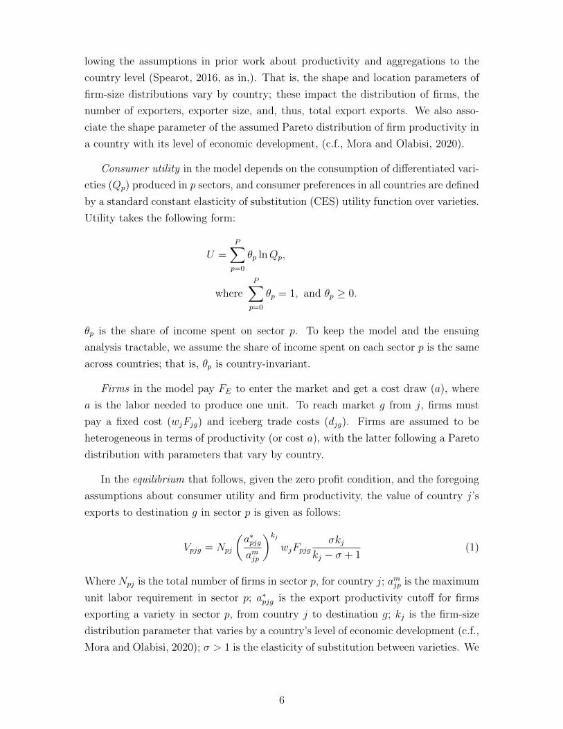
In the equilibrium that follows, given the zero profit condition, and the foregoing
assumptions about consumer utility and firm productivity, the value of country j’s
exports to destination g in sector p is given as follows:
Vpjg = Npj
(a∗pjgamjp
)kjwjFpjg
σkjkj − σ + 1
(1)
Where Npj is the total number of firms in sector p, for country j; amjp is the maximum
unit labor requirement in sector p; a∗pjg is the export productivity cutoff for firms
exporting a variety in sector p, from country j to destination g; kj is the firm-size
distribution parameter that varies by a country’s level of economic development (c.f.,
Mora and Olabisi, 2020); σ > 1 is the elasticity of substitution between varieties. We
6
will show that these variables, particularly σ and kj, not only impact total exports,
but also affect how countries respond to trade shocks.
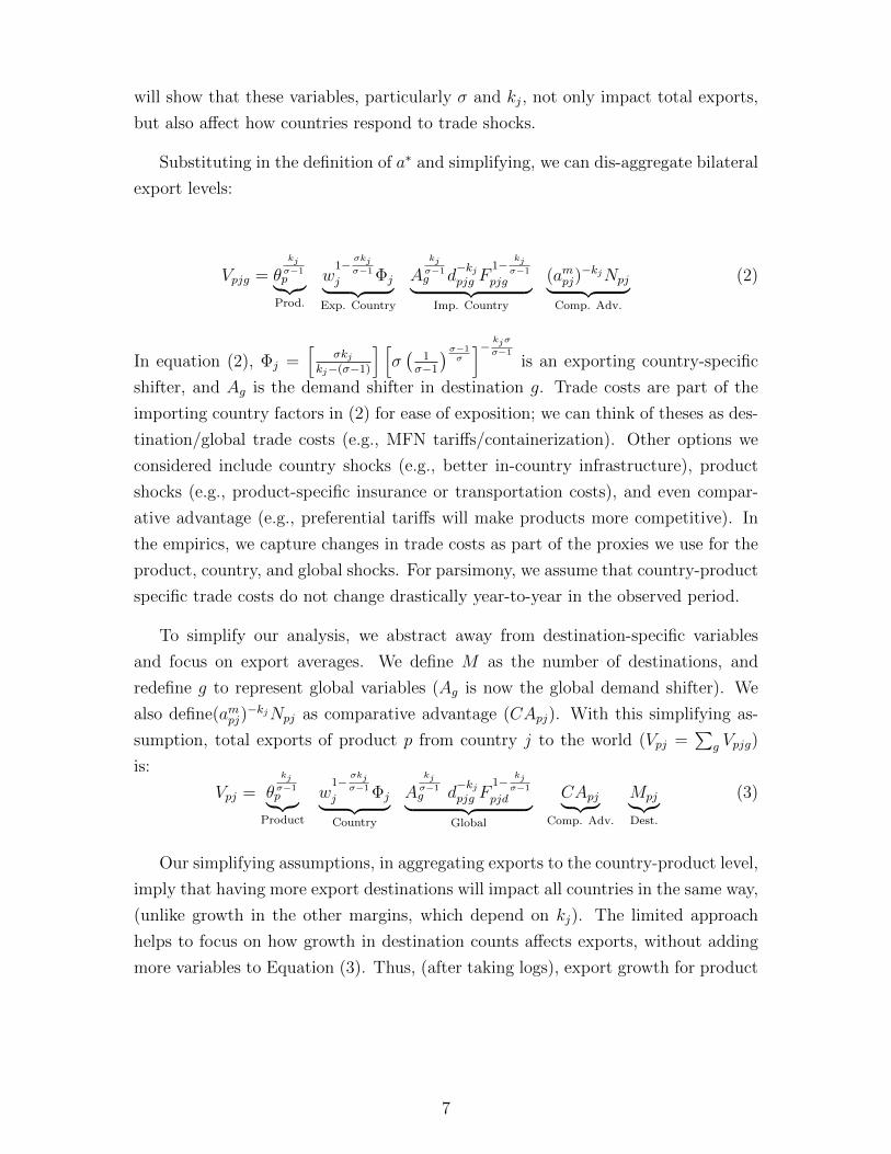
Substituting in the definition of a∗ and simplifying, we can dis-aggregate bilateral
export levels:
Vpjg = θkjσ−1p︸︷︷︸
Prod.
w1−
σkjσ−1
j Φj︸ ︷︷ ︸Exp. Country
Akjσ−1g d
−kjpjg F
1−kjσ−1
pjg︸ ︷︷ ︸Imp. Country
(ampj)−kjNpj︸ ︷︷ ︸
Comp. Adv.
(2)
In equation (2), Φj =[
σkjkj−(σ−1)
] [σ(
1σ−1
)σ−1σ
]− kjσ
σ−1
is an exporting country-specific
shifter, and Ag is the demand shifter in destination g. Trade costs are part of the
importing country factors in (2) for ease of exposition; we can think of theses as des-
tination/global trade costs (e.g., MFN tariffs/containerization). Other options we
considered include country shocks (e.g., better in-country infrastructure), product
shocks (e.g., product-specific insurance or transportation costs), and even compar-
ative advantage (e.g., preferential tariffs will make products more competitive). In
the empirics, we capture changes in trade costs as part of the proxies we use for the
product, country, and global shocks. For parsimony, we assume that country-product
specific trade costs do not change drastically year-to-year in the observed period.
To simplify our analysis, we abstract away from destination-specific variables
and focus on export averages. We define M as the number of destinations, and
redefine g to represent global variables (Ag is now the global demand shifter). We
also define(ampj)−kjNpj as comparative advantage (CApj). With this simplifying as-
sumption, total exports of product p from country j to the world (Vpj =∑
g Vpjg)
is:
Vpj = θkjσ−1p︸︷︷︸
Product
w1−
σkjσ−1
j Φj︸ ︷︷ ︸Country
Akjσ−1g d
−kjpjg F
1−kjσ−1
pjd︸ ︷︷ ︸Global
CApj︸ ︷︷ ︸Comp. Adv.
Mpj︸︷︷︸Dest.
(3)
Our simplifying assumptions, in aggregating exports to the country-product level,
imply that having more export destinations will impact all countries in the same way,
(unlike growth in the other margins, which depend on kj). The limited approach
helps to focus on how growth in destination counts affects exports, without adding
more variables to Equation (3). Thus, (after taking logs), export growth for product
7
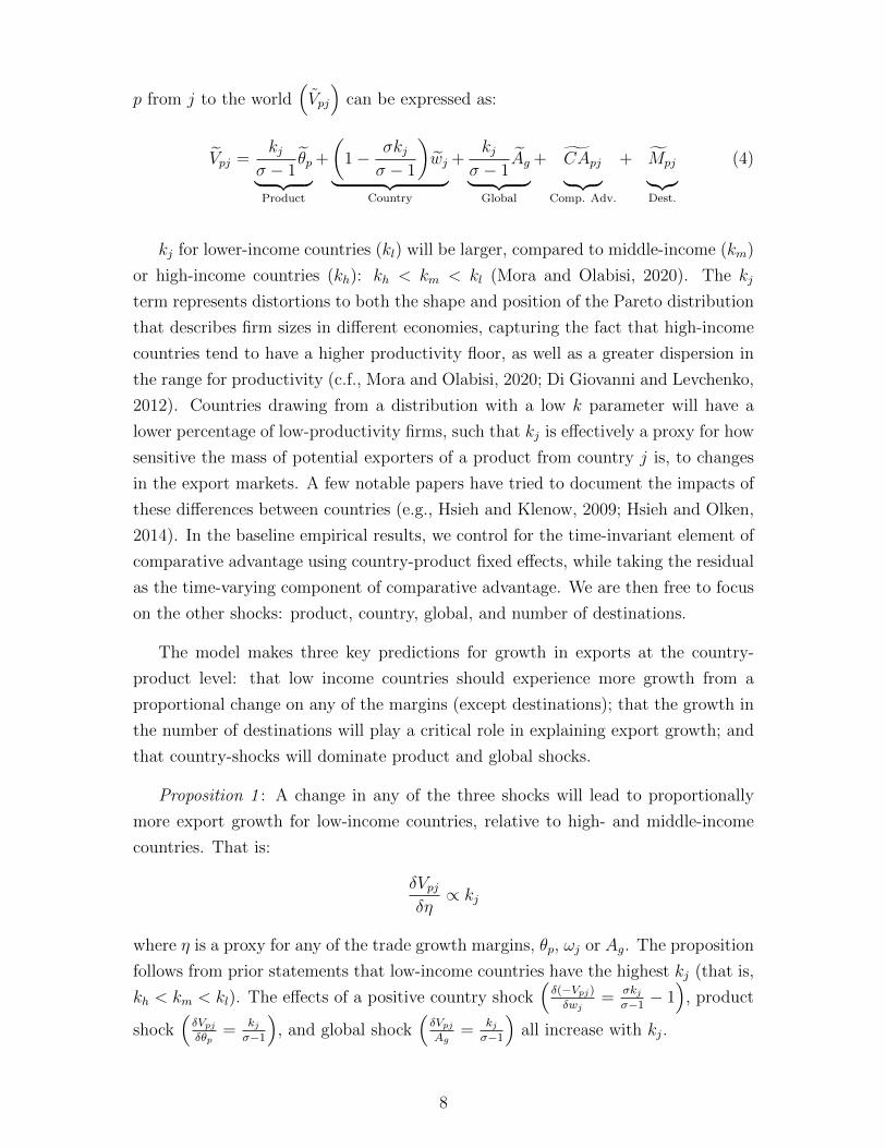
p from j to the world(Vpj
)can be expressed as:
Vpj =kj
σ − 1θp︸ ︷︷ ︸
Product
+
(1− σkj
σ − 1
)wj︸ ︷︷ ︸
Country
+kj
σ − 1Ag︸ ︷︷ ︸
Global
+ CApj︸ ︷︷ ︸Comp. Adv.
+ Mpj︸︷︷︸Dest.
(4)
kj for lower-income countries (kl) will be larger, compared to middle-income (km)
or high-income countries (kh): kh < km < kl (Mora and Olabisi, 2020). The kj
term represents distortions to both the shape and position of the Pareto distribution
that describes firm sizes in different economies, capturing the fact that high-income
countries tend to have a higher productivity floor, as well as a greater dispersion in
the range for productivity (c.f., Mora and Olabisi, 2020; Di Giovanni and Levchenko,
2012). Countries drawing from a distribution with a low k parameter will have a
lower percentage of low-productivity firms, such that kj is effectively a proxy for how
sensitive the mass of potential exporters of a product from country j is, to changes
in the export markets. A few notable papers have tried to document the impacts of
these differences between countries (e.g., Hsieh and Klenow, 2009; Hsieh and Olken,
2014). In the baseline empirical results, we control for the time-invariant element of
comparative advantage using country-product fixed effects, while taking the residual
as the time-varying component of comparative advantage. We are then free to focus
on the other shocks: product, country, global, and number of destinations.
The model makes three key predictions for growth in exports at the country-
product level: that low income countries should experience more growth from a
proportional change on any of the margins (except destinations); that the growth in
the number of destinations will play a critical role in explaining export growth; and
that country-shocks will dominate product and global shocks.
Proposition 1 : A change in any of the three shocks will lead to proportionally
more export growth for low-income countries, relative to high- and middle-income
countries. That is:
δVpjδη∝ kj
where η is a proxy for any of the trade growth margins, θp, ωj or Ag. The proposition
follows from prior statements that low-income countries have the highest kj (that is,
kh < km < kl). The effects of a positive country shock(δ(−Vpj)δwj
=σkjσ−1− 1)
, product
shock(δVpjδθp
=kjσ−1
), and global shock
(δVpjAg
=kjσ−1
)all increase with kj.
8
Developing countries are expected to be more sensitive to export markets, given
their greater values for kj, i.e., share of the mass of firms having productivity levels
below the exporting threshold. The firm-size distribution relative to the export
productivity threshold implies that an exogenous positive shock in global demand,
or to costs and productivity at the country-level – which we term global, product, or
country shocks, will stimulate more new exporters and higher export growth rates
in countries with high kj values, all else equal.
Proposition 2 : Growth in the number of destinations, everything else being equal,
will move in unison with growth in exports:
δVpjδM
' 1
While the number of destinations reached by a country may depend on the level
of economic development, the effect of a proportional increase in destinations will
not depend on the level of economic development. According to Equation 4, with
increasing numbers of export destinations for each product p, export values grow at
approximately the same rate, (barring distortions from variables, including kj, that
affect the value of Mpj).
Proposition 3 : For all countries, export growth will be more responsive to country
shocks, compared to product shocks. That is:
σ(kj − 1) + 1
σ − 1>
kjσ − 1
The scale factor in (4) associated with a positive country shock, wj < 0, is equal
toσkjσ−1− 1, compared to that for a proportional, positive product/global shock
kjσ−1
.
As the elasticity of substitution and the position parameter are greater than one
(σ > 1 and kj > 1 ), the country shock should have a greater impact on exports than
the other shocks, given the same kj. One policy implication of this prediction, is
that developing economies looking for export growth are more likely to succeed with
policies that broadly address export competitiveness and destination diversification,
rather than a focus on selecting or promoting successful products.
9
III Data and Descriptives
From theory to empirics: We use proxies for the variables in Equation 4 to capture
the shocks described in the previous section: [1] The global shock (Ag), is measured as
growth in world exports in non-p products (minus those from country j): V ∗gt = Agt;
[2] the product shock (θp) is measured as the growth in world exports of product p
(minus those from country j), V ∗pt, minus the global shock: V ∗
pt = V ∗pt− V ∗
gt = θpt, that
is, we can only have a positive shock if exports of that product grow at a greater
rate than that of overall world exports; [3] the country shock (wj), own-country en-
vironment, is replaced with growth in total exports from country j (minus exports in
product p), V ∗jt, minus the global shock: V ∗
jt = V ∗jt− V ∗
gt = −wjt, here, as for the prod-
uct shock, we can only have a positive shock in a country if exports of that country
grow at a greater rate faster than that of overall world exports; [4] the comparative
advantage shock, which we represent as the combination of constant trend changes
(a term, Ωpj, represents country-product fixed effects), and time-varying effects from
the regression residual term. Trade costs, be they country (eg, infrastructure im-
provements), product (eg. MFN tariffs), or global (eg. lower transportation costs),
are captured by our proxies; with this method, the only trade costs we don’t capture
are those that are country-product specific. The only directly observable variable in
our data is the growth in the exports destinations (Mpjt).
With our proxies, we can express Equation 4 as follows:
Vpjt = Ωpj︸︷︷︸Comp. Adv.
+kj
σ − 1V ∗pt︸ ︷︷ ︸
Product
+
(σkjσ − 1
− 1
)V ∗jt︸ ︷︷ ︸
Country
+kj
σ − 1V ∗gt︸ ︷︷ ︸
Global
+ Mpjt︸ ︷︷ ︸Dest.
(5)
In the following section, we take Equation 5 and trade data from the BACI database
to test the predictions of the model.
III.a Data
We use the BACI database for product-level international trade, developed by the
Centre d’etudes prospectives et d’informations internationales (CEPII). The dataset
is best described as the UN COMTRADE data at the 6-digit disaggregation level,
harmonized to the 1992 HS schedule definitions, and with bilateral reporting differ-
10
ences in trade reconciled.3 We have 21 years of data, 1995 to 2015. To match the
data to the model, we collapse the export data to the country-product-year level.
We define country groups based on the World Bank categories for economic de-
velopment: low-income, middle-income, or high-income. The original World Bank
classification scheme had five categories, which we summarized to three: 1) 53 low-
income countries, 2) 90 middle-income countries (includes lower-middle income and
upper-middle income countries), and 3) 45 high-income countries (includes high-
income OECD and high-income non-OECD countries). See Table A.1 for a complete
list of the countries and income categories.
To compare broad sectors across countries, we concorded the more than 5,000
HS 6-digit product (HS-6) definitions to 10 SITC product sectors. The broad sector
groups for analysis was motivated by the data. High-income countries are more
likely to have the advantage in terms of industrial and manufactured goods, while
low income countries tend to have comparative advantage in extractive industries and
the agricultural sector, much like the evidence in a long-running body of literature
(e.g., Balassa, 1979; Redding, 2002; Bernard, Redding, and Schott, 2007).
We lose a few observations to our data-cleaning process. We drop reporting
countries that do not have observations in every available year and drop HS products
that do not convert to SITC Rev. 3 product categories. Additionally, because
we organize countries by their level of economic development in the World Bank
classification scheme, we drop countries not classified by the World Bank. The
restrictions leave us with 183 countries – about 97% of our original observations, or
data losses that we consider minor.
III.b Descriptives
We identify margins of export growth that highlight the significant variation observed
in the data at the product-level. Figure A.1 shows that 2015 exports were higher
than 1995 exports for most products, at the narrowly-defined HS6 level, but the
growth ratio was higher than 10 for more than one hundred products (e.g., analog
wristwatches, diesel-electric locomotives), while global exports declined for more than
500 products, with a few declining all the way to zero in 2015 (e.g., cassette tapes -
HS 852421, and whole bovine skin leather - HS410410). This variation in the data for
3For a description of the procedure developed to reconcile the data, see Gaulier and Zignago(2010).
11

us, motivates an inquiry into how much of the observed historical growth in exports
is explained by product-specific trends, or by the other margins of trade growth,
after accounting for products.
Our motivation to revisit the ‘what drives export growth’ question, and to develop
a model with new margins of trade, rests largely on the data. Many of the products
whose exports fell over time, like cassette tapes, dropped because of changing tastes
and technology. Such changes do not affect all countries equally. Similarly, not all
countries gained from the boom in computer exports, so it becomes important to
explore how much of export growth is due to exporting the right products, compared
to other potential drivers of export growth.
The second panel of Figure A.1 highlights how export growth at the country-level
also varies significantly. Fewer than ten countries increased exports by more than
a factor of 50 between 1995 and 2015, but the most common increase was near the
global average of 3.4. Exports declined for more than twenty countries. As posited
earlier, the open question is, how much of the change can be attributed to the country,
not just to product or aggregate trends. With the foregoing, do we expect that the
rising tide of global trade lifts all countries? Or do we have some countries that do
particularly well? Or are the changes limited to some sectors and products?
Sector Composition and Economic Development
The patterns in Figure A.1 depend on economic development. The figure shows
what share of the countries in each growth bin belongs to the LICs, MICs or HICs
categories. First, high-income countries’ exports cover a broader range of products,
as documented in related papers on export growth (e.g., Hummels and Klenow, 2005;
Kehoe and Ruhl, 2013). Second, low income countries have more instances of product
exports declining to zero, noted in the early literature as the extensive margin of
trade (Besedes and Prusa, 2011; Cadot et al., 2011). They also have more instances
of exports increasing by a factor of 50 or more over two decades in the data, consistent
with other papers that document the big hits in exports (Freund and Pierola, 2012;
Cadot, Disdier, Jaud, and Suwa-Eisenmann, 2014). Middle income countries seem
to lie in the middle of the patterns for high-income and the lowest-income countries.
As exports for middle-income countries grew faster than high-income countries, on
average, by 2015, high income economies, even after 20 years of average positive
trade growth, had less than 60% of the global export market.
12
We observe notable changes in the global export shares of country-groups, as
well as changes in the sector composition of their exports. Table 1 shows the sector
composition of export growth – both the importance of each sector for the country-
groups, as well as changes to their shares of global exports between 1995 and 2015.
The sector composition of exports changed for low-income countries, challenging
the low-income commodity-exporter narrative. For the group, the sector with the
highest growth was sector 7 (Machinery and transport equipment), increasing by
13.7 percentage points from 4.4% of exports from the group in 1995. By comparison,
sector 8 increased by 5.3 percentage points, to remain the largest export sector
by value. Sector 0 (Food and live animals) and sector 6 (Manufactured goods)
saw significant decreases in the share of low income countries’ exports, -7.5 and -
9.5 percentage points respectively. Low-income countries also improved their global
export market share by almost 3 percentage points, more than doubling from their
2% share of global exports in 1995. The sector-level summaries reveal a pattern
of broadly positive, if uneven growth. The countries improved market share in all
sectors, ranging from increases of 1.2 percentage points for Sector 4 (Oils, fats and
waxes) to 5.8 percentage points for Sector 8 (Miscellaneous manufactured articles).
Middle-income countries improved even more than low-income countries – in-
creasing their global export market share by an impressive 18 percentage points,
almost doubling their 1996 share of 19.4%. In the sector-level detail data, we see
broad growth and increasing shares of global exports across the full range of sectors,
ranging from 2.2 for items not classified, to 27.9 percentage points for Sector 7 (Ma-
chinery and transport equipment). While the data clearly shows significant changes
in the sector composition of exports for middle-income countries, the changes appear
to differ from those of low-income countries. The sector with the greatest increase in
export market share for middle-income countries is also the sector with the greatest
global export growth in the period; sector 7, which increased from 23% to 39% of
MICs’ exports. Sector 0 (Food and live animals) and sector 6 (Manufactured goods)
saw significant decreases in export share, -4 and -4.6 percentage points respectively.
For HICs, the sector composition of exports varied little. The most notable
changes include the smaller share of exports from Sectors 6, 7, and 8, falling 3.9, 6.3,
and 1.1 percentage points respectively. The sector with the most increase in high-
income country export shares is Sector 3 (5.1 percentage points), followed closely
by Sector 5 (Chemicals and related products). Furthermore, high-income countries
(HICs) lost a non-trivial share of global exports (20.7 percentage points) in the
13
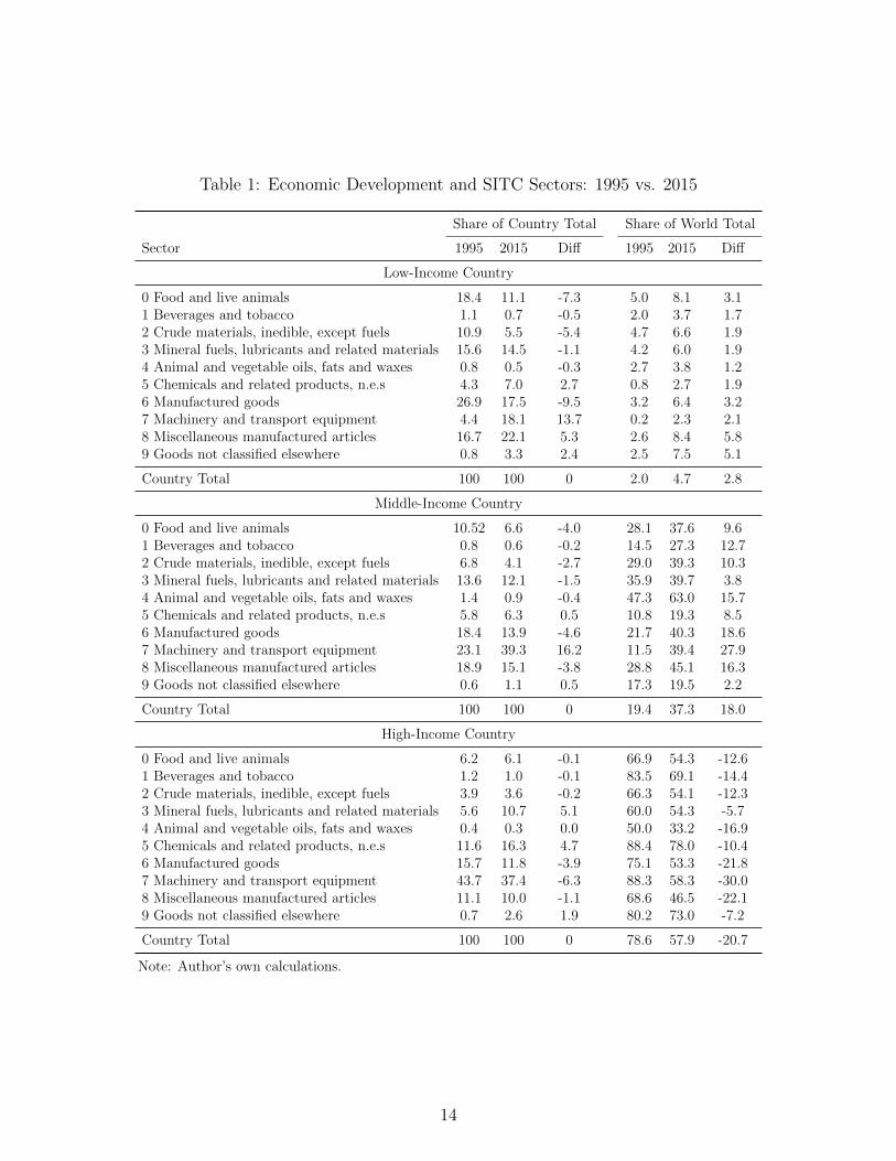
Table 1: Economic Development and SITC Sectors: 1995 vs. 2015
Share of Country Total Share of World Total
Sector 1995 2015 Diff 1995 2015 Diff
Low-Income Country
0 Food and live animals 18.4 11.1 -7.3 5.0 8.1 3.11 Beverages and tobacco 1.1 0.7 -0.5 2.0 3.7 1.72 Crude materials, inedible, except fuels 10.9 5.5 -5.4 4.7 6.6 1.93 Mineral fuels, lubricants and related materials 15.6 14.5 -1.1 4.2 6.0 1.94 Animal and vegetable oils, fats and waxes 0.8 0.5 -0.3 2.7 3.8 1.25 Chemicals and related products, n.e.s 4.3 7.0 2.7 0.8 2.7 1.96 Manufactured goods 26.9 17.5 -9.5 3.2 6.4 3.27 Machinery and transport equipment 4.4 18.1 13.7 0.2 2.3 2.18 Miscellaneous manufactured articles 16.7 22.1 5.3 2.6 8.4 5.89 Goods not classified elsewhere 0.8 3.3 2.4 2.5 7.5 5.1
Country Total 100 100 0 2.0 4.7 2.8
Middle-Income Country
0 Food and live animals 10.52 6.6 -4.0 28.1 37.6 9.61 Beverages and tobacco 0.8 0.6 -0.2 14.5 27.3 12.72 Crude materials, inedible, except fuels 6.8 4.1 -2.7 29.0 39.3 10.33 Mineral fuels, lubricants and related materials 13.6 12.1 -1.5 35.9 39.7 3.84 Animal and vegetable oils, fats and waxes 1.4 0.9 -0.4 47.3 63.0 15.75 Chemicals and related products, n.e.s 5.8 6.3 0.5 10.8 19.3 8.56 Manufactured goods 18.4 13.9 -4.6 21.7 40.3 18.67 Machinery and transport equipment 23.1 39.3 16.2 11.5 39.4 27.98 Miscellaneous manufactured articles 18.9 15.1 -3.8 28.8 45.1 16.39 Goods not classified elsewhere 0.6 1.1 0.5 17.3 19.5 2.2
Country Total 100 100 0 19.4 37.3 18.0
High-Income Country
0 Food and live animals 6.2 6.1 -0.1 66.9 54.3 -12.61 Beverages and tobacco 1.2 1.0 -0.1 83.5 69.1 -14.42 Crude materials, inedible, except fuels 3.9 3.6 -0.2 66.3 54.1 -12.33 Mineral fuels, lubricants and related materials 5.6 10.7 5.1 60.0 54.3 -5.74 Animal and vegetable oils, fats and waxes 0.4 0.3 0.0 50.0 33.2 -16.95 Chemicals and related products, n.e.s 11.6 16.3 4.7 88.4 78.0 -10.46 Manufactured goods 15.7 11.8 -3.9 75.1 53.3 -21.87 Machinery and transport equipment 43.7 37.4 -6.3 88.3 58.3 -30.08 Miscellaneous manufactured articles 11.1 10.0 -1.1 68.6 46.5 -22.19 Goods not classified elsewhere 0.7 2.6 1.9 80.2 73.0 -7.2
Country Total 100 100 0 78.6 57.9 -20.7
Note: Author’s own calculations.
14
1995–2015 period. The HICs lost export market share in all sectors, with the largest
decrease (30 percentage points) in sector 7 and the smallest decline (5.7 percentage
points) in sector 3 (Mineral fuels, lubricants and related materials).
In sum, Table 1 shows how trade changed over time, as well as how the changes
could have occurred. Country-shocks common to many developing countries could
have increased exports across all sectors, and it could be that the developing countries
that added sector 7 to their export portfolios enjoyed more growth as the world
demanded more machinery and transport equipment.
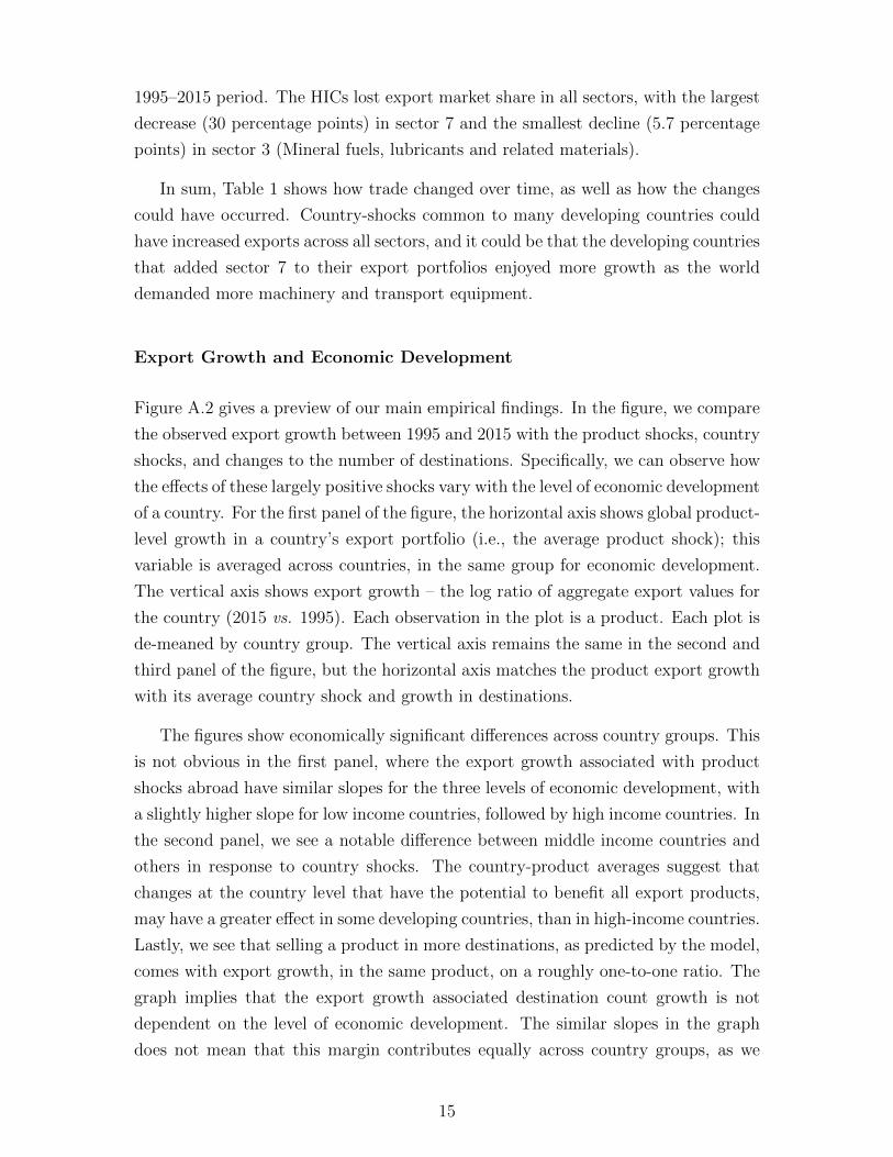
Export Growth and Economic Development
Figure A.2 gives a preview of our main empirical findings. In the figure, we compare
the observed export growth between 1995 and 2015 with the product shocks, country
shocks, and changes to the number of destinations. Specifically, we can observe how
the effects of these largely positive shocks vary with the level of economic development
of a country. For the first panel of the figure, the horizontal axis shows global product-
level growth in a country’s export portfolio (i.e., the average product shock); this
variable is averaged across countries, in the same group for economic development.
The vertical axis shows export growth – the log ratio of aggregate export values for
the country (2015 vs. 1995). Each observation in the plot is a product. Each plot is
de-meaned by country group. The vertical axis remains the same in the second and
third panel of the figure, but the horizontal axis matches the product export growth
with its average country shock and growth in destinations.
The figures show economically significant differences across country groups. This
is not obvious in the first panel, where the export growth associated with product
shocks abroad have similar slopes for the three levels of economic development, with
a slightly higher slope for low income countries, followed by high income countries. In
the second panel, we see a notable difference between middle income countries and
others in response to country shocks. The country-product averages suggest that
changes at the country level that have the potential to benefit all export products,
may have a greater effect in some developing countries, than in high-income countries.
Lastly, we see that selling a product in more destinations, as predicted by the model,
comes with export growth, in the same product, on a roughly one-to-one ratio. The
graph implies that the export growth associated destination count growth is not
dependent on the level of economic development. The similar slopes in the graph
does not mean that this margin contributes equally across country groups, as we
15
will explore later. Developing countries have expanded the number of their export
destinations more than high income countries.
In the empirics, we test the relationship between export growth at the country-
product level and each of the listed growth shocks.
IV Empirics
We begin with an empirical model derived from Equations (4) and (5), to explain
export growth for product p from country j at time t:
Vpjt = β0 + β1V∗pt + β2 V
∗jt + β3V
∗t + β4Mpjt + Ωpj + εpjt (6)
Where, β1 is the estimated effect of an external product shock(V ∗pt
), β2 is
the estimated effect of a change in the exporting country’s export competitiveness(V ∗jt
), β3 is the estimated effect of a global shock
(V ∗t
), and β4 is the estimated
effect of growing the number of destinations(M∗
pjt
). Ωpj captures country-product
fixed effects and is our proxy for the time-invariant comparative advantage com-
ponents. εpjt is the error term, which effectively captures the elements of com-
parative advantage that change from year to year. As described in the previous
section, we define the growth shock components, or margins, for country j export-
ing product p as: V ∗t =
2∗∑i 6=j
∑q 6=p(Vqit−Vqit−1)∑
i6=j∑q 6=p(Vqit+Vqit−1)
, V ∗pt =
2∗∑i 6=j(Vpit−Vpit−1)∑i6=j(Vpit+Vpit−1)
− V ∗t , and
V ∗jt =
2∗∑q 6=p(Vqjt−Vqjt−1)∑q 6=p(Vqjt+Vqjt−1)
− V ∗t .4
All four β terms are expected to be positive, as well as the comparative advantage
measure that includes the residual and Ωpj. We test for differences between developed
and developing countries, by using interactions with country-group dummy variables
for the β1, β2, and β3 terms.5 Equation 6 is similar to the revealed comparative
advantage (RCA) equation, with variables similarly defined, except that we exclude
country j exports and add destination growth (c.f., Balassa, 1979).
The model, as stated earlier, predicts the following: [1] similar shocks will affect
4We don’t include year fixed-effects in Equation (6) as the global shock mostly captures the yeareffects; unsurprisingly, there is little variation, within a year, for the global shock across countries.Including year fixed effects has minimal impact on the estimated effect of the product and countryshocks.
5Although we don’t show it in the baseline estimates, we also interact β4 with country-groupdummy variables as a robustness check.
16
countries differently, depending on their level of economic development: βpoori >
βrichi , ∀i = 1, 2, 3; [2] β4, the effect of increasing the number of destinations, is not
dependent on the level of economic development and should be equal to one; and [3]
country shocks matter more than product shocks for all countries; β2 > β1, β3. This
distinction is important as it implies that institutional differences effect how exports
grow in the countries, and also to what extent they benefit from globalization.6
IV.a Baseline Results: Annual Export Growth
Table 2 provides the baseline estimates for Equation 6. Column 1 shows that export
growth (for country-product combinations) increases with global product shocks in
the same year after controlling for country product fixed effects. We see that a 1
percent increase in aggregate product demand results in an estimated 0.36 percent
increase in exports of the same product. Changing the specification to include coun-
try shocks (Column 2) lowers the correlation between product shocks and export
growth slightly, while adding country and global shocks raises the estimated corre-
lation between export growth and product shocks. Positive country shocks predict
higher HS 6-digit product exports (see column 3); while exports have a stronger link
to the country shock variable (0.6), than to product shocks (0.4). The global shocks
variable, as expected, also has a positive effect.
Specifications that extend Equation 6 to include interaction terms with the coun-
try groups, reveal interesting differences between high-income and developing coun-
tries. The shock variables (product, country, and global) are interacted with dummies
for high-income countries and low-income countries, leaving middle-income countries
as the omitted baseline (see column 4). The dummy variables highlight notable differ-
ences between countries at different stages of economic development, some of which
is explained by the growth in the number of export destinations, as shown in column
5 of the table. First, the estimated effects of product shocks and country shocks di-
minish once we account for export destination growth, with middle-income countries
having estimates of 0.11 for product shocks and 0.12 for country shocks. Product
shocks for low-income and high-income countries are estimated to be 0.03 percent
lower and 0.04 percent higher respectively.
Country shocks, on the other hand, have a stronger link to exports for middle-
income countries, more than high-income and even more than low-income countries.
6We remove country j exports to avoid having the same export values in multiple variables andto avoid bias from having the same trade flow on both the right and left hand sides of the equation.
17
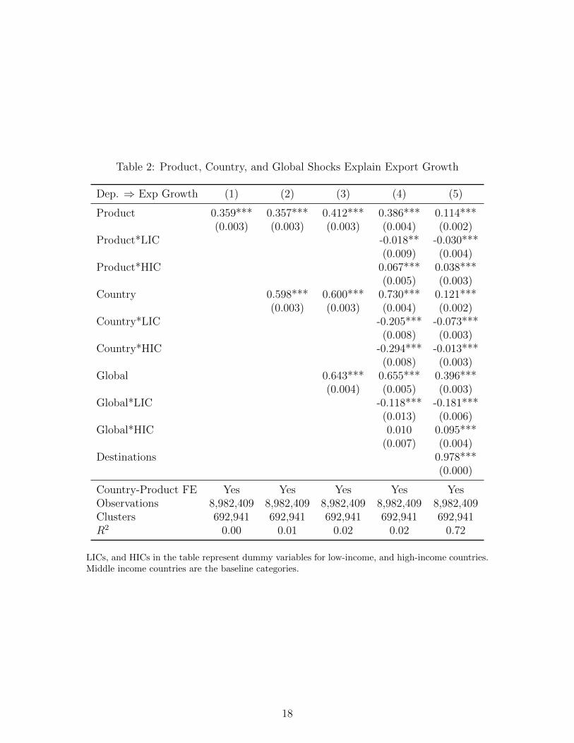
Table 2: Product, Country, and Global Shocks Explain Export Growth
Dep. ⇒ Exp Growth (1) (2) (3) (4) (5)
Product 0.359*** 0.357*** 0.412*** 0.386*** 0.114***(0.003) (0.003) (0.003) (0.004) (0.002)
Product*LIC -0.018** -0.030***(0.009) (0.004)
Product*HIC 0.067*** 0.038***(0.005) (0.003)
Country 0.598*** 0.600*** 0.730*** 0.121***(0.003) (0.003) (0.004) (0.002)
Country*LIC -0.205*** -0.073***(0.008) (0.003)
Country*HIC -0.294*** -0.013***(0.008) (0.003)
Global 0.643*** 0.655*** 0.396***(0.004) (0.005) (0.003)
Global*LIC -0.118*** -0.181***(0.013) (0.006)
Global*HIC 0.010 0.095***(0.007) (0.004)
Destinations 0.978***(0.000)
Country-Product FE Yes Yes Yes Yes YesObservations 8,982,409 8,982,409 8,982,409 8,982,409 8,982,409Clusters 692,941 692,941 692,941 692,941 692,941R2 0.00 0.01 0.02 0.02 0.72
LICs, and HICs in the table represent dummy variables for low-income, and high-income countries.Middle income countries are the baseline categories.
18
While the former fits the model’s prediction, the latter suggests that structural bar-
riers not included in our model assumptions diminish export growth in low income
countries. As outlined in Mora and Olabisi (2020), having fewer firms and at the
same time, a greater share of firms below the Melitz-style productivity threshold
for exports, means that low-income countries should be more responsive to drivers
of export growth. In principle, a larger share of resident firms make the transition
into exports with such positive shocks, as implied by the kj term in Equation (4).
So, a country-wide shock like trade reforms that increase exports across all prod-
ucts, should be more of a stimulus for export growth in a low-income country like
Bangladesh, relative to a high-income country like Belgium.
Global shocks show larger estimated effects on exports than either product or
country shocks, with the effect being lower for low-income and higher for high-income
economies. The higher estimated effects for global and product shocks may imply
that firms in high-income countries are not as constrained as in developing countries,
and can take advantage of sudden changes in demand than the theory predicts – both
for product shocks and global shocks. That said, our interpretation of the estimate
for this estimate comes with the caveat that it may be biased – the skewed nature
of trade, where 20% of countries account for more than 70% of exports, mean that
our measure of global shocks are not uniform across countries.7
Lastly, growth in the number of destinations decreases the effect of the product,
country and global shocks (in column 5). It also increases the model’s ability to
explain the variation in export growth (R2 jumps to .72). This implies that some of
the gains from product-shocks and country-shocks translate to growth in the number
of destinations for country-product combinations. Once we account for growth in the
number of markets served by exporters of a product from a given country, the effects
of the global shock overtakes those of product- and country shocks. Even if the sizes
of the estimated coefficients decrease, the signs and statistical significance of the
difference-in-difference estimates remain largely consistent.
7The deviation from the model’s predictions for the estimated effects of product and global shocksmay imply that the same constraints that shape the firm-size distributions and lead to larger kjs indeveloping economies, may work outside the firm size distribution to prevent export growth. Forproduct shocks, the observed estimates may simply be a reflection of portfolio size. The averagenumbers of HS6 products in 2015 export portfolios was roughly 1,100, 2,100 and 3,100 for LICS,MICS and HICs respectively. Having more items in the export portfolio means greater exposure toproduct shocks. It may also be that most export surges related to changing tastes consolidate themarket shares of the incumbent market leaders, who are mre likely to be in high-income countries.
19
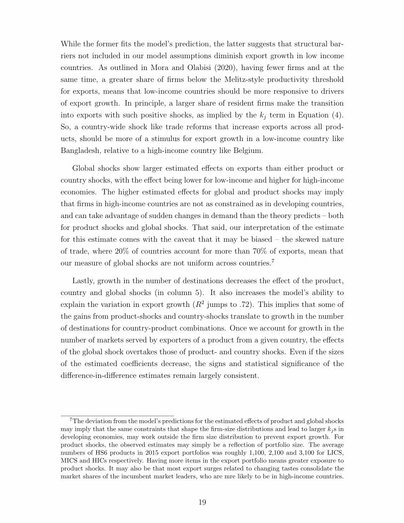
Table 3: Product, Country, and World Shocks Explain Export Growth: SITC Sectors
Dep. ⇒ Exp Growth Sect 0 Sect 1 Sect 2 Sect 3 Sect 4 Sect 5 Sect 6 Sect 7 Sect 8 Sect 9
Product 0.141*** 0.043 0.150*** 0.081*** 0.145*** 0.126*** 0.116*** 0.096*** 0.074*** 0.059*(0.006) (0.034) (0.006) (0.016) (0.015) (0.005) (0.003) (0.004) (0.004) (0.032)
Product*LIC -0.050*** 0.023 0.001 -0.023 -0.051 -0.035*** -0.033*** -0.041*** -0.009 -0.062(0.012) (0.064) (0.012) (0.029) (0.033) (0.012) (0.007) (0.008) (0.009) (0.054)
Product*HIC 0.016* 0.130** 0.006 0.042* 0.056*** 0.013* 0.042*** 0.069*** 0.036*** 0.020(0.009) (0.051) (0.009) (0.025) (0.021) (0.007) (0.005) (0.007) (0.006) (0.049)
Country 0.104*** 0.125*** 0.044*** 0.109*** 0.098*** 0.111*** 0.130*** 0.142*** 0.119*** 0.058(0.006) (0.020) (0.008) (0.023) (0.021) (0.005) (0.004) (0.004) (0.004) (0.058)
Country*LIC -0.064*** -0.039 -0.011 -0.003 -0.068** -0.047*** -0.083*** -0.090*** -0.073*** -0.034(0.009) (0.031) (0.013) (0.039) (0.033) (0.009) (0.006) (0.006) (0.007) (0.084)
Country*HIC 0.004 -0.070* 0.039** -0.036 -0.027 -0.002 -0.012* -0.029*** -0.016** -0.164*(0.011) (0.037) (0.016) (0.044) (0.038) (0.009) (0.007) (0.007) (0.007) (0.095)
Global 0.368*** 0.373*** 0.526*** 0.700*** 0.479*** 0.406*** 0.453*** 0.363*** 0.290*** 0.267***(0.009) (0.039) (0.013) (0.041) (0.034) (0.008) (0.006) (0.007) (0.007) (0.101)
Global*LIC -0.115*** -0.151* -0.121*** -0.320*** -0.142** -0.172*** -0.221*** -0.233*** -0.113*** 0.040(0.018) (0.079) (0.025) (0.086) (0.069) (0.017) (0.011) (0.013) (0.013) (0.170)
Global*HIC 0.068*** 0.027 0.070*** 0.017 0.117** 0.145*** 0.096*** 0.101*** 0.057*** 0.231(0.014) (0.059) (0.019) (0.063) (0.050) (0.012) (0.008) (0.010) (0.010) (0.149)
Destinations 0.973*** 0.971*** 0.970*** 0.971*** 0.979*** 0.980*** 0.977*** 0.985*** 0.975*** 0.965***(0.000) (0.002) (0.001) (0.002) (0.001) (0.000) (0.000) (0.000) (0.000) (0.004)
Country-Product FE Yes Yes Yes Yes Yes Yes Yes Yes Yes YesObservations 938,772 62,627 541,925 58,982 74,839 1,220,495 2,498,579 1,907,872 1,666,194 12,124Clusters 72,685 4,388 44,740 4,805 6,287 98,993 196,996 140,427 122,672 948R2 0.71 0.69 0.72 0.69 0.73 0.74 0.73 0.71 0.71 0.65
LICs, and HICs in the table represent dummy variables for low-income, and high-income countries. Middle income countries are the baseline categories.
20
The estimated effects of growth shocks are broadly similar across SITC sectors in
Table 3, especially when focusing on the manufacturing sectors (Sector 6 – 8). While
the difference-in-difference effects for the product and world shock are similar for the
agricultural and resource sectors (Sectors 0 – 3), the estimates are not statistically
significant. This is unsurprising, in part because the regressions in Table 3 control
for time-invariant comparative advantage through the use of product-country fixed
effects.
The shocks yield positive and statistically significant effects on growth across
most sectors in Table 3. Country shocks for middle-income countries are larger
in magnitude than product shocks for half of the 10 sectors, (the exceptions are
Sectors 0, 2, 4, 5, 9). The estimated effect of product shocks on Sector 1 (Beverages
and Tobacco), and of country shocks on Sector 9, are positive but not statistically
significant. Global secular growth appears to drive export growth more than either a
similar product or country shocks, across the sectors, as in the last column of Table
2. As discussed for column 5 of Table 2, product shocks and global shocks have a
higher impact for high-income countries, than for the developing economies. Finally,
destination growth explains most of the variation in export growth for all sectors,
just as it provides the largest predicted response (other than comparative advantage,
which is not shown in the table).
Predicted contributions to export growth: Table 4 shows the predicted share of
export growth from each of the margins in our model. The estimates are derived
from a version of Table 3 that is specific to country groups, where the coefficients
are multiplied by the observed proxy for each of the margins to generate the ex-
pected contribution to growth. At this point, we also estimate the contribution of
comparative advantage, i.e., the observed export growth minus the contributions of
the product, country, world, and destination shocks. To aggregate the contribution
for each of the shocks to the country-group level, we calculate the trade-weighted-
average, across time and countries, of the various margins. Finally, to calculate the
shares reported in the table, we take the trade-weighted average contributions and
divide them by the observed trade-weighted average export growth for the country
group and sector. Each row in the table represents one set of linear regression esti-
mates, equivalent to a column in Table 3 for the subset of countries in each country
group. The sector and country-level aggregates are reported separately for each of
the country groups by level of economic development.
Table 4 follows expectations, as it translates the estimated regression coefficients,
21
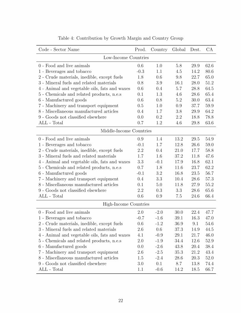
Table 4: Contribution by Growth Margin and Country Group
Code - Sector Name Prod. Country Global Dest. CA
Low-Income Countries
0 - Food and live animals 0.6 1.0 5.8 29.9 62.61 - Beverages and tobacco -0.3 1.1 4.5 14.2 80.62 - Crude materials, inedible, except fuels 1.8 0.6 9.8 22.7 65.03 - Mineral fuels and related materials 0.8 3.9 16.1 28.0 51.24 - Animal and vegetable oils, fats and waxes 0.6 0.4 5.7 28.8 64.55 - Chemicals and related products, n.e.s 0.1 1.3 4.6 28.6 65.46 - Manufactured goods 0.6 0.8 5.2 30.0 63.47 - Machinery and transport equipment 0.5 1.0 0.9 37.7 59.98 - Miscellaneous manufactured articles 0.4 1.7 3.8 29.9 64.29 - Goods not classified elsewhere 0.0 0.2 2.2 18.8 78.8ALL - Total 0.7 1.2 4.6 29.8 63.6
Middle-Income Countries
0 - Food and live animals 0.9 1.4 13.2 29.5 54.91 - Beverages and tobacco -0.1 1.7 12.8 26.6 59.02 - Crude materials, inedible, except fuels 2.2 0.4 21.0 17.7 58.83 - Mineral fuels and related materials 1.7 1.6 37.2 11.8 47.64 - Animal and vegetable oils, fats and waxes 3.3 -0.1 17.9 16.8 62.15 - Chemicals and related products, n.e.s 0.7 1.8 11.6 23.7 62.26 - Manufactured goods -0.1 3.2 16.8 23.5 56.77 - Machinery and transport equipment 0.4 3.3 10.4 28.6 57.38 - Miscellaneous manufactured articles 0.1 5.0 11.8 27.9 55.29 - Goods not classified elsewhere 2.2 0.3 3.3 28.6 65.6ALL - Total 0.6 0.9 7.5 24.6 66.4
High-Income Countries
0 - Food and live animals 2.0 -2.0 30.0 22.4 47.71 - Beverages and tobacco -0.7 -1.6 39.1 16.3 47.02 - Crude materials, inedible, except fuels 0.6 -1.2 36.9 9.1 54.63 - Mineral fuels and related materials 2.6 0.6 37.3 14.9 44.54 - Animal and vegetable oils, fats and waxes 4.1 -0.9 29.1 21.7 46.05 - Chemicals and related products, n.e.s 2.0 -1.9 34.4 12.6 52.96 - Manufactured goods 0.0 -2.6 43.8 20.4 38.47 - Machinery and transport equipment 2.6 -2.5 35.3 21.2 43.48 - Miscellaneous manufactured articles 1.5 -2.4 28.6 20.3 52.09 - Goods not classified elsewhere 3.0 0.1 8.7 13.8 74.4ALL - Total 1.1 -0.6 14.2 18.5 66.7
22
using what we know about trade growth. Product shocks contributed the least to
export growth in developing economies. For high-income economies, product shocks
contributed more than than country shocks, but still represented less than 2.5% of
all growth, with notable variation between sectors. The findings are consistent with
the top panel of Figure A.1, which shows exports for most products grew between
1995 and 2015, but only about half grew faster than the 3.4 ratio that was the global
average for the period. Combining the coefficients for product shocks (which were
the smallest of all the margins), with the small product shocks described in the
Figure, gives the expected low contribution of product shocks to aggregate growth.
In the low-income countries (LICs), the contribution of product shocks ranged from
-0.3% for the Beverages and Tobacco sector, as commodities like coffee and cocoa
saw increased price competition, to 1.8% for the crude materials sector, where other
commodities saw booms in demand from countries like China.
The higher coefficients for country shocks (relative to product shocks, even if less
than destination growth or global shocks), with the observed country shocks gives
the expected result that country shocks contributed more than product shocks to
export growth in developing economies in Table 4. Evidence for higher observed
country shocks is in the second panel of Figure A.1, which shows that exports for
most countries grew between 1995 and 2015, with about 60% of countries growing
faster than the 3.4 ratio that was the secular global average for the period.
Destination growth and global shocks contributed more than country or product
shocks to export growth across all country groups in Table 4. The findings suggest
that efforts focused on ‘what you export’ or national competitiveness have limited
effects on prompting above-average export growth, outside of complementary efforts
to sustain growth in the number of destinations. Secular growth over time accounted
for nearly 5% of growth in low-income economies – in a pattern that varied across
sectors, from a low of 0.9% for except for Sector 7 (Machinery and transport equip-
ment) to a high of 16.1% for Sector 3 (Mineral fuels and related materials). The
impact of global shocks differ for other country groups, accounting for 14.2% and
33.4% of growth for MICs and HICs, respectively, but with the highest impact for
HICs is in Sector 6 (Manufactured goods). The implication is that export growth in
a time of global trade recession is unlikely for any country or sector, especially if the
country is a high-income country.
A notable share of export growth cannot be explained by the margins we proposed
– product shocks, country shocks, global shocks, and destination growth. The com-
23
parative advantage term in our framework (captured by the residual combined with
the country-product fixed effects), explains the greatest share of export growth in
the data. About two-thirds of export growth in low-income, 60% of that in middle-
income, and 50% of that in high-income economies all come from factors specific
to country-product combinations. The contributions of comparative advantage vary
across sectors within the country-groups. Comparative advantage, which for example
may relate to ability of Cote d’Ivoire to produce cocoa, accounted for 80% of export
growth in sector 1 (Beverages and tobacco) for LICs, while the comparable number
for MICs and HICs was less than 60%. The contribution of comparative advantage
was highest for animal fats and chemicals sectors (4 and 5) in MICs , while it was
highest in HICs for sectors 2 and 5 (Crude materials, and Chemicals). We ignored
Sector 9 - Goods not classified elsewhere, in making the comparisons. The finding
that comparative advantage contributes the most to export growth is notable, but
not surprising.
Discussion: The results in Tables 2, 3, and 4 suggest that successful export growth
strategies cannot rely on finding products that are big hits. The leading contributors
to export growth in developing economies are efforts to find new destinations, as
well as country-product-specific factors that drive comparative advantage, much like
the firm-level productivity gains described in much of the empirical trade literature.
For high income countries, the mix is different: the leading contributors to export
growth are the secular global growth trend, and comparative advantage. Higher
destination numbers contribute to export growth for high-income countries, but not
at the same level as for developing countries. The reason for this is not hard to
deduce, high-income countries served more destinations ab initio, with the average
number of destinations reached with each product in 1995 at 4, 6 and 22 respectively
for LICs, MICs and HICs. Doubling the number of destinations from a finite set is
easier from a smaller base, like the LICs had in 1995.
Policy that enhances national export competitiveness across all products is more
likely to succeed in promoting exports, compared to chasing positive product shocks,
even if country-specific drivers are not the biggest observed contributor to export
growth in the past two decades. The results show that the dominance of country
shocks over product shocks is clearest for the countries and sectors that experienced
the greatest growth in the last two decades.
The contribution of global shocks in Table 4 implies one difference in growth
strategies for LICs, compared with HICs: global export downturns are less of a
24
barrier (and, also, less of a benefit) to growth for low-income countries than their
wealthier counterparts. This idea is consistent with other papers that suggest trade
in low income countries does not significantly respond to world income (e.g., Freund,
2009; Kose and Prasad, 2011). The sectoral regressions also show that exports for
some sectors (e.g., manufactured goods) are more sensitive to global growth shocks
than others (e.g., miscellaneous manufactured articles). Similarly, the contributions
of comparative advantage in the table implies that across country groups and sectors,
policies that create local advantage consistently support export growth.
IV.b Robustness Checks
Our findings remain largely robust to multiple definitions of export growth rates (see
Table 5). The first set of results repeats the findings in Table 2, with midpoint growth
rates; ”Midpoint 2” used the same growth rate measurement, but doesn’t delete own
country/product/country-product exports from the shock variables; “Avg” method
uses the simple growth rate equation to calculate growth; “∆Arsinh” calculates
the growth using inverse hyperbolic sine, which allows us to double the number of
observations by including country-product-year triads with missing zero values; and
“∆log” calculates growth rates using the difference in logged values.
The simple growth rate and hyper-sine specifications lead to big changes in the
number of observations, as observations with zero trade get dropped (or included).
When accounting for zero values, the estimated effects decrease and the difference-
in-difference effect for the global shock switches sign for high-income countries. That
said, the estimated coefficients of destination count growth are positive, statistically
significant and close to 1, for all three specifications linked to log growth. The
estimated coefficients are statistically significant for three, and positive for four of the
five specifications, while the country shocks are positive and statistically significant
for four of the five specifications. As predicted, country shock estimates are greater
than product shock estimates in all but one specification.
In continuing the robustness checks, Table 6 uses long-run growth from 1995 to
2015 as the dependent variable. This reduces the number of observations in the
regressions to the less than half-a-million unique non-zero country-product combi-
nations in the data. (The observations increase to almost a million when zero-trade
linkages are included, as in columns 4 and 5). The column definitions are identical
to Table 5, with an additional column for log differences with one added in levels, to
25
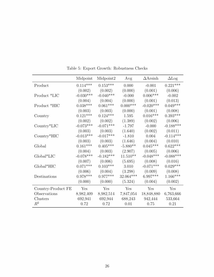
Table 5: Export Growth: Robustness Checks
Midpoint Midpoint2 Avg ∆Arsinh ∆Log
Product 0.114*** 0.153*** 0.000 -0.001 0.221***(0.002) (0.002) (0.000) (0.001) (0.006)
Product *LIC -0.030*** -0.040*** -0.000 0.006*** -0.002(0.004) (0.004) (0.000) (0.001) (0.013)
Product *HIC 0.038*** 0.061*** 0.000*** -0.020*** 0.049***(0.003) (0.003) (0.000) (0.001) (0.008)
Country 0.121*** 0.124*** 1.595 0.016*** 0.393***(0.002) (0.002) (1.389) (0.002) (0.006)
Country*LIC -0.073*** -0.071*** -1.797 -0.000 -0.188***(0.003) (0.003) (1.640) (0.002) (0.011)
Country*HIC -0.013*** -0.017*** -1.810 0.004 -0.114***(0.003) (0.003) (1.646) (0.004) (0.010)
Global 0.161*** 0.405*** -5.880** 0.045*** 0.622***(0.004) (0.003) (2.907) (0.005) (0.006)
Global*LIC -0.078*** -0.182*** 11.510** -0.048*** -0.088***(0.007) (0.006) (5.695) (0.008) (0.016)
Global*HIC 0.071*** 0.103*** 3.010 -0.071*** 0.029***(0.006) (0.004) (3.298) (0.009) (0.008)
Destinations 0.978*** 0.977*** 32.064*** 6.997*** 1.166***(0.000) (0.000) (5.324) (0.004) (0.002)
Country-Product FE Yes Yes Yes Yes YesObservations 8,982,409 8,982,514 7,847,054 18,848,880 6,763,666Clusters 692,941 692,944 688,243 942,444 533,664R2 0.72 0.72 0.01 0.75 0.21
26
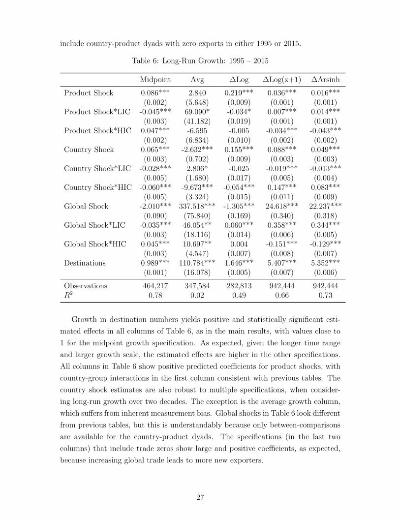
include country-product dyads with zero exports in either 1995 or 2015.
Table 6: Long-Run Growth: 1995 – 2015
Midpoint Avg ∆Log ∆Log(x+1) ∆Arsinh
Product Shock 0.086*** 2.840 0.219*** 0.036*** 0.016***(0.002) (5.648) (0.009) (0.001) (0.001)
Product Shock*LIC -0.045*** 69.090* -0.034* 0.007*** 0.014***(0.003) (41.182) (0.019) (0.001) (0.001)
Product Shock*HIC 0.047*** -6.595 -0.005 -0.034*** -0.043***(0.002) (6.834) (0.010) (0.002) (0.002)
Country Shock 0.065*** -2.632*** 0.155*** 0.088*** 0.049***(0.003) (0.702) (0.009) (0.003) (0.003)
Country Shock*LIC -0.028*** 2.806* -0.025 -0.019*** -0.013***(0.005) (1.680) (0.017) (0.005) (0.004)
Country Shock*HIC -0.060*** -9.673*** -0.054*** 0.147*** 0.083***(0.005) (3.324) (0.015) (0.011) (0.009)
Global Shock -2.010*** 337.518*** -1.305*** 24.618*** 22.237***(0.090) (75.840) (0.169) (0.340) (0.318)
Global Shock*LIC -0.035*** 46.054** 0.060*** 0.358*** 0.344***(0.003) (18.116) (0.014) (0.006) (0.005)
Global Shock*HIC 0.045*** 10.697** 0.004 -0.151*** -0.129***(0.003) (4.547) (0.007) (0.008) (0.007)
Destinations 0.989*** 110.784*** 1.646*** 5.407*** 5.352***(0.001) (16.078) (0.005) (0.007) (0.006)
Observations 464,217 347,584 282,813 942,444 942,444R2 0.78 0.02 0.49 0.66 0.73
Growth in destination numbers yields positive and statistically significant esti-
mated effects in all columns of Table 6, as in the main results, with values close to
1 for the midpoint growth specification. As expected, given the longer time range
and larger growth scale, the estimated effects are higher in the other specifications.
All columns in Table 6 show positive predicted coefficients for product shocks, with
country-group interactions in the first column consistent with previous tables. The
country shock estimates are also robust to multiple specifications, when consider-
ing long-run growth over two decades. The exception is the average growth column,
which suffers from inherent measurement bias. Global shocks in Table 6 look different
from previous tables, but this is understandably because only between-comparisons
are available for the country-product dyads. The specifications (in the last two
columns) that include trade zeros show large and positive coefficients, as expected,
because increasing global trade leads to more new exporters.
27
V Conclusion
The last two decades witnessed a remarkable increase in global trade, with developing
countries increasing their share of global goods exports. The pattern of increasing
trade was not uniform, and for developing economies the differences raise the broad
question of whether lessons from past export growth episodes can shape future growth
strategies. Understanding the drivers of export growth matters, because knowing
how exports and income levels increased in economies like China and Colombia can
be useful for economies where export growth is needed to stimulate economic growth.
In this paper we take a new approach to defining how country-level exports grow.
The framework helps us to assess export growth and how each of the following
reasons contribute: [a] a country exports during good economic times, when demand
and exports are growing for all products (a global shock); [b] a country increases
exports of a specific product in its export portfolio when technology or tastes drive
up demand for the product, even when other products are not growing (a product
shock); [c] a country improves comparative advantage for a product, so that its export
growth for the product is higher than average (comparative advantage shock), [d] a
country adopts policies designed to increase exports across the broad spectrum of
products in its portfolio, e.g., trade facilitation and reduction (a country shock), or
[e] a country expands its existing export portfolio to new markets. Exports growing
primarily because of factors internal to a country means that policymakers can make
a difference by committing to initiatives that increase the exports of all products from
the country (c.f., Freund and Pierola, 2015), or making investments that increase
their comparative advantage on a product-by-product basis.
We develop a heterogeneous-firm theoretical model that guides our thinking about
the link between the aforementioned margins and exports at the country-product
level. The model also explains how the links are affected by a country’s stage of
economic development. We estimate the correlation between the trade margins and
export values (as well as growth), using BACI data. We find positive associations
between exports and some of the trade shocks (or margins).
Discussion: Using the theory to guide our empirics, we test how growth shocks
(product, country, and global) and the addition of export destinations are associ-
ated with own country exports after controlling for trend changes in comparative
advantage, and whether or not this association depends on the level of economic
development. As mentioned earlier, differences in the link between the growth mar-
28
gins and the level of economic development will have important policy implications.
For example, how should countries, especially developing ones, spend limited gov-
ernment resources in attempts to improve exports? For example, countries could
focus on improving external market access, facilitating exports for preferred prod-
ucts, or enhancing the country’s advantage for a narrow set of products/sectors.
Alternatively, countries could be more broadly focused on polices that benefit all ex-
ports; for example, infrastructure improvements, ease of starting a business, export
licensing restrictions. Lastly, it may be that export growth depends on the global
environment, and the role of government in promoting exports is minimal; meaning
government policy should not even focus on policies specific to the exporting sector.
We find that countries at different stages of economic development generally have
different drivers of export growth. Relative to middle-income countries, product
and global shocks are more important in driving exports for high-income countries,
and less so for low-income countries. At the same time, country shocks are more
important for middle income countries’ exports, and less so for high-income and low-
income countries. Finally, the addition of export markets is an important driver in
export growth, and a main driver in the observed export growth.
The findings matter for policy: In the first place, policy initiatives and national-
level factors matter for trade growth, as earlier papers demonstrate for economic
growth (e.g., Snowberg, Wolfers, and Zitzewitz, 2007; Jones and Olken, 2005). For
better or worse, for developing countries, country-level factors explain export growth
better than product-level factors in our analysis. This implies that in the short
term, developing countries could benefit from inward-looking policies that help all
exporters, rather than trying to catch waves of export product booms. Notably,
we find a strong connection between growth and the number of export destinations,
which makes the case for efforts to improve market access abroad, and resonates with
prior work that links growth to export diversification (Eicher and Kuenzel, 2016).
Our findings also caution developing countries against emulating high-income coun-
tries’ growth strategies. Low income countries do not benefit as much from exogenous
positive demand shocks relative to their high-income peers (product or global). Our
model suggests that institutional differences and barriers shape firm-level growth and
firm-size distributions, and thus limit the responsiveness of developing countries to
export opportunities. Therefore, policies that reduce the growth constraints on firms
in the developing world could generate substantial export growth.
29
References
Amiti, Mary and Caroline Freund (2010), “The Anatomy of China’s Export Growth.”In China’s Growing Role in World Trade, 35–56, University of Chicago Press.
Balassa, Bela (1979), “The Changing Pattern of Comparative Advantage in Manu-factured Goods.” Review of Economics and Statistics, 259–266.
Baliamoune-Lutz, Mina (2011), “Growth by Destination (Where You Export Mat-ters): Trade With China and Growth in African Countries.” African DevelopmentReview, 23, 202–218.
Bastos, Paulo and Joana Silva (2010), “The Quality of a Firm’s Exports: WhereYou Export to Matters.” Journal of International Economics, 82, 99–111.
Bernard, Andrew B, Stephen J Redding, and Peter K Schott (2007), “ComparativeAdvantage and Heterogeneous Firms.” Review of Economic Studies, 74, 31–66.
Besedes, Tibor and Thomas J Prusa (2011), “The Role of Extensive and IntensiveMargins and Export Growth.” Journal of Development Economics, 96, 371–379.
Brambilla, Irene, Daniel Lederman, and Guido Porto (2012), “Exports, Export Des-tinations, and Skills.” American Economic Review, 102, 3406–38.
Broda, Christian and David E Weinstein (2006), “Globalization and the Gains fromVariety.” Quarterly Journal of Economics, 121, 541–585.
Cadot, Olivier, Celine Carrere, and Vanessa Strauss-Kahn (2011), “Export Diver-sification: What’s Behind the Hump?” Review of Economics and Statistics, 93,590–605.
Cadot, Olivier, Anne-Celia Disdier, Melise Jaud, and Akiko Suwa-Eisenmann (2014),“Export Big Hits.” Technical report, International Growth Center.
Chaney, Thomas (2008), “Distorted Gravity: The Intensive and Extensive Marginsof International Trade.” American Economic Review, 98, 1707–21.
Chang, Roberto, Linda Kaltani, and Norman V. Loayza (2009), “Openness Can BeGood for Growth: The Role of Policy Complementarities.” Journal of DevelopmentEconomics, 90, 33–49.
Di Giovanni, Julian and Andrei A Levchenko (2012), “Country Size, InternationalTrade, and Aggregate Fluctuations in Granular Economies.” Journal of PoliticalEconomy, 120, 1083–1132.
Eaton, Jonathan, Marcela Eslava, Maurice Kugler, and James Tybout (2007), “Ex-port Dynamics in Colombia: Firm-Level Evidence.” Technical report, NationalBureau of Economic Research.
Eaton, Jonathan, Samuel Kortum, and Francis Kramarz (2011), “An Anatomy ofInternational Trade: Evidence From French Firms.” Econometrica, 79, 1453–1498.
30
Egger, Peter and Jan Prusa (2016), “The Determinants of Trade Costs: A RandomCoefficient Approach.” Empirical Economics, 50, 51–58.
Egger, Peter H and Sergey Nigai (2015), “Structural Gravity With Dummies Only:Constrained ANOVA-Type Estimation of Gravity Models.” Journal of Interna-tional Economics, 97, 86–99.
Egger, Peter H and Sergey Nigai (2016), “World-Trade Growth Accounting.” CESifoWorking Paper Series.
Eicher, Theo S and David J Kuenzel (2016), “The elusive effects of trade on growth:Export diversity and economic take-off.” Canadian Journal of Economics/Revuecanadienne d’economique, 49, 264–295.
Feenstra, Robert C and Shang-Jin Wei (2010), China’s Growing Role in World Trade.University of Chicago Press.
Freund, Caroline (2009), “The Trade Response to Global Downturns.” In The GreatTrade Collapse: Causes, Consequences and Prospects (Richard Baldwin, ed.), 59–70, CEPR.
Freund, Caroline and Martha Denisse Pierola (2012), “Export Surges.” Journal ofDevelopment Economics, 97, 387–395.
Freund, Caroline and Martha Denisse Pierola (2015), “Export Superstars.” Reviewof Economics and Statistics, 97, 1023–1032.
Gaulier, Guillaume and Soledad Zignago (2010), “BACI: International TradeDatabase at the Product-Level (The 1994-2007 Version).” CEPII Working Paper2010-23.
Hanson, Gordon H (2012), “The Rise of Middle Kingdoms: Emerging Economies inGlobal Trade.” Journal of Economic Perspectives, 26, 41–64.
Harrison, A (1996), “Openness and Growth: A Time-Series, Cross-Country Analysisfor Developing Countries.” Journal of Development Economics, 48, 419–447.
Hausmann, Ricardo, Jason Hwang, and Dani Rodrik (2007), “What You ExportMatters.” Journal of Economic Growth, 12, 1–25.
Hidalgo, Cesar A, Bailey Klinger, A-L Barabasi, and Ricardo Hausmann (2007),“The Product Space Conditions the Development of Nations.” Science, 317, 482–487.
Hsieh, Chang-Tai and Peter J Klenow (2009), “Misallocation and ManufacturingTFP in China and India.” Quarterly Journal of Economics, 124, 1403–1448.
Hsieh, Chang-Tai and Benjamin A Olken (2014), “The Missing ”Missing Middle”.”Journal of Economic Perspectives, 28, 89–108.
31
Hummels, David and Peter J Klenow (2005), “The Variety and Quality of a Nation’sExports.” American Economic Review, 95, 704–723.
Imbs, Jean and Romain Wacziarg (2003), “Stages of Diversification.” American Eco-nomic Review, 93, 63–86.
Jones, Benjamin F and Benjamin A Olken (2005), “Do Leaders Matter? NationalLeadership and Growth Since World War II.” Quarterly Journal of Economics,120, 835–864.
Kehoe, Timothy J and Kim J Ruhl (2013), “How Important Is the New GoodsMargin in International Trade?” Journal of Political Economy, 121, 358–392.
Koren, Miklos and Silvana Tenreyro (2013), “Technological Diversification.” Ameri-can Economic Review, 103, 378–414.
Kose, M Ayhan and Eswar S Prasad (2011), Emerging Markets: Resilience andGrowth Amid Global Turmoil. Brookings Institution Press.
Mora, Jesse and Michael Olabisi (2020), “Economic Development and the Marginsof Trade: Are the Least Developed Countries Different?” Economic Inquiry.
Newfarmer, Richard, William Shaw, and Peter Walkenhorst (2009), Breaking IntoNew Markets: Emerging Lessons for Export Diversification. The World Bank.
Onder, Ali Sina and Hakan Yilmazkuday (2016), “Trade Partner Diversification andGrowth: How Trade Links Matter.” Journal of Macroeconomics, 50, 241–258.
Parteka, Aleksandra and Massimo Tamberi (2013), “Product Diversification, Rela-tive Specialisation and Economic Development: Import-Export Analysis.” Journalof Macroeconomics, 38, 121–135.
Redding, Stephen (2002), “Specialization Dynamics.” Journal of International Eco-nomics, 58, 299–334.
Rose, Andrew K (2007), “The Foreign Service and Foreign Trade: Embassies asExport Promotion.” World Economy, 30, 22–38.
Schott, Peter K (2008), “The Relative Sophistication of Chinese Exports.” EconomicPolicy, 23, 6–49.
Snowberg, Erik, Justin Wolfers, and Eric Zitzewitz (2007), “Partisan Impacts onthe Economy: Evidence From Prediction Markets and Close Elections.” QuarterlyJournal of Economics, 122, 807–829.
Spearot, Alan (2016), “Unpacking the Long-run Effects of Tariff Shocks: New Struc-tural Implications from Firm Heterogeneity Models.” American Economic Journal:Microeconomics, 8, 128–67.
Ventura, J (1997), “Growth and Interdependence.” Quarterly Journal of Economics,112, 57–84.
32
Zymek, Robert (2015), “Factor Proportions and the Growth of World Trade.” Jour-nal of International Economics, 95, 42–53.
33
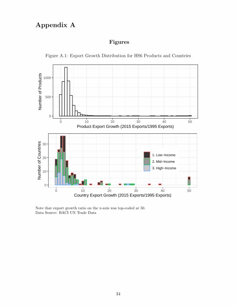
Appendix A
Figures
Figure A.1: Export Growth Distribution for HS6 Products and Countries
0
500
1000
0 10 20 30 40 50
Product Export Growth (2015 Exports/1995 Exports)
Num
ber
of P
rodu
cts
0
10
20
30
0 10 20 30 40 50Country Export Growth (2015 Exports/1995 Exports)
Num
ber
of C
ount
ries
1. Low−Income
2. Mid−Income
3. High−Income
Note that export growth ratio on the x-axis was top-coded at 50.Data Source: BACI UN Trade Data
34
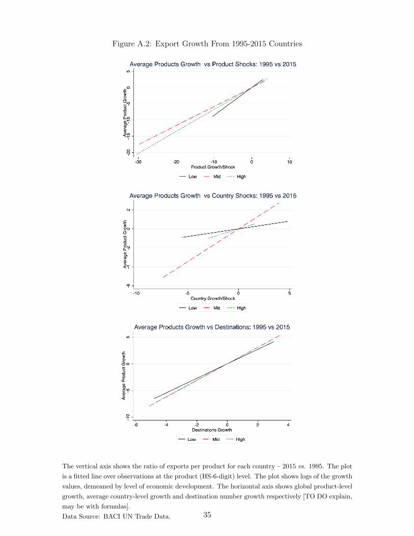
Figure A.2: Export Growth From 1995-2015 Countries
The vertical axis shows the ratio of exports per product for each country – 2015 vs. 1995. The plot
is a fitted line over observations at the product (HS-6-digit) level. The plot shows logs of the growth
values, demeaned by level of economic development. The horizontal axis shows global product-level
growth, average country-level growth and destination number growth respectively [TO DO explain,
may be with formulas].
Data Source: BACI UN Trade Data. 35
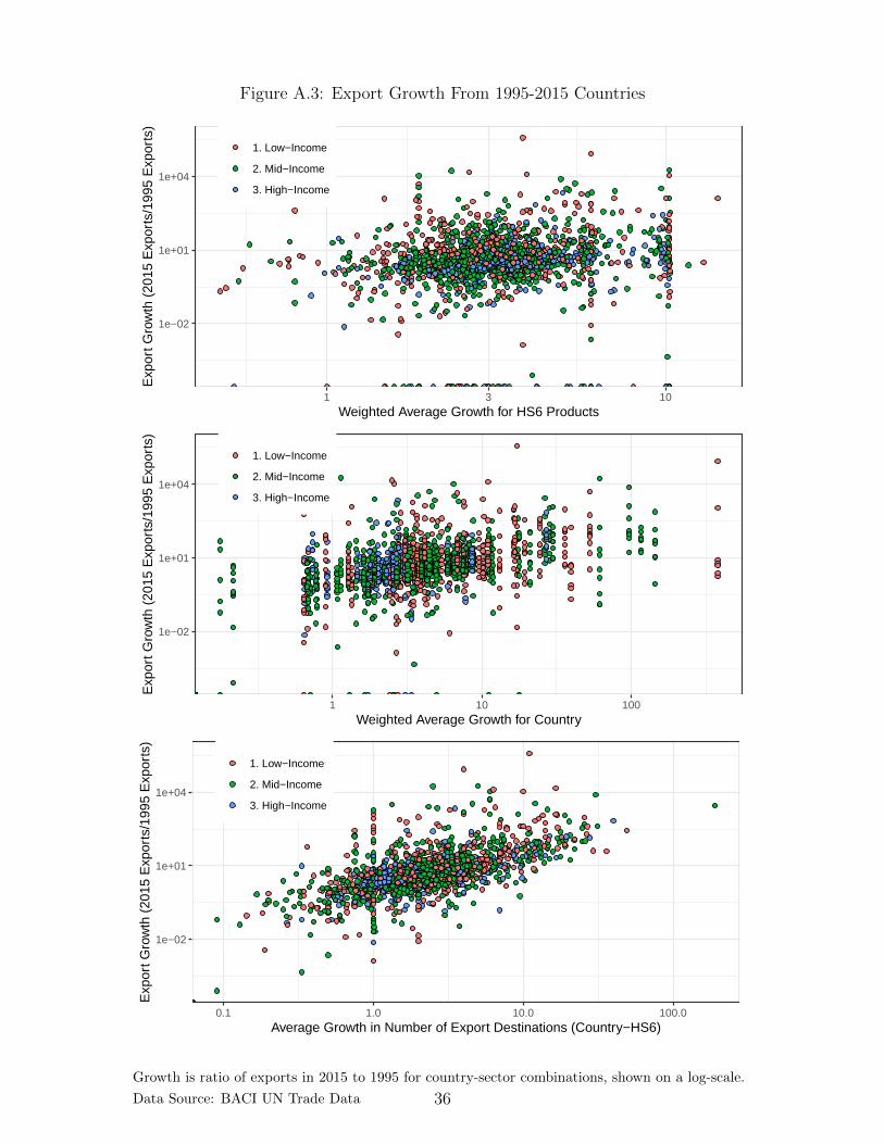
Figure A.3: Export Growth From 1995-2015 Countries
1e−02
1e+01
1e+04
1 3 10Weighted Average Growth for HS6 Products
Exp
ort G
row
th (
2015
Exp
orts
/199
5 E
xpor
ts)
1. Low−Income
2. Mid−Income
3. High−Income
1e−02
1e+01
1e+04
1 10 100Weighted Average Growth for Country
Exp
ort G
row
th (
2015
Exp
orts
/199
5 E
xpor
ts)
1. Low−Income
2. Mid−Income
3. High−Income
1e−02
1e+01
1e+04
0.1 1.0 10.0 100.0Average Growth in Number of Export Destinations (Country−HS6)
Exp
ort G
row
th (
2015
Exp
orts
/199
5 E
xpor
ts)
1. Low−Income
2. Mid−Income
3. High−Income
Growth is ratio of exports in 2015 to 1995 for country-sector combinations, shown on a log-scale.
Data Source: BACI UN Trade Data 36

Tables
37
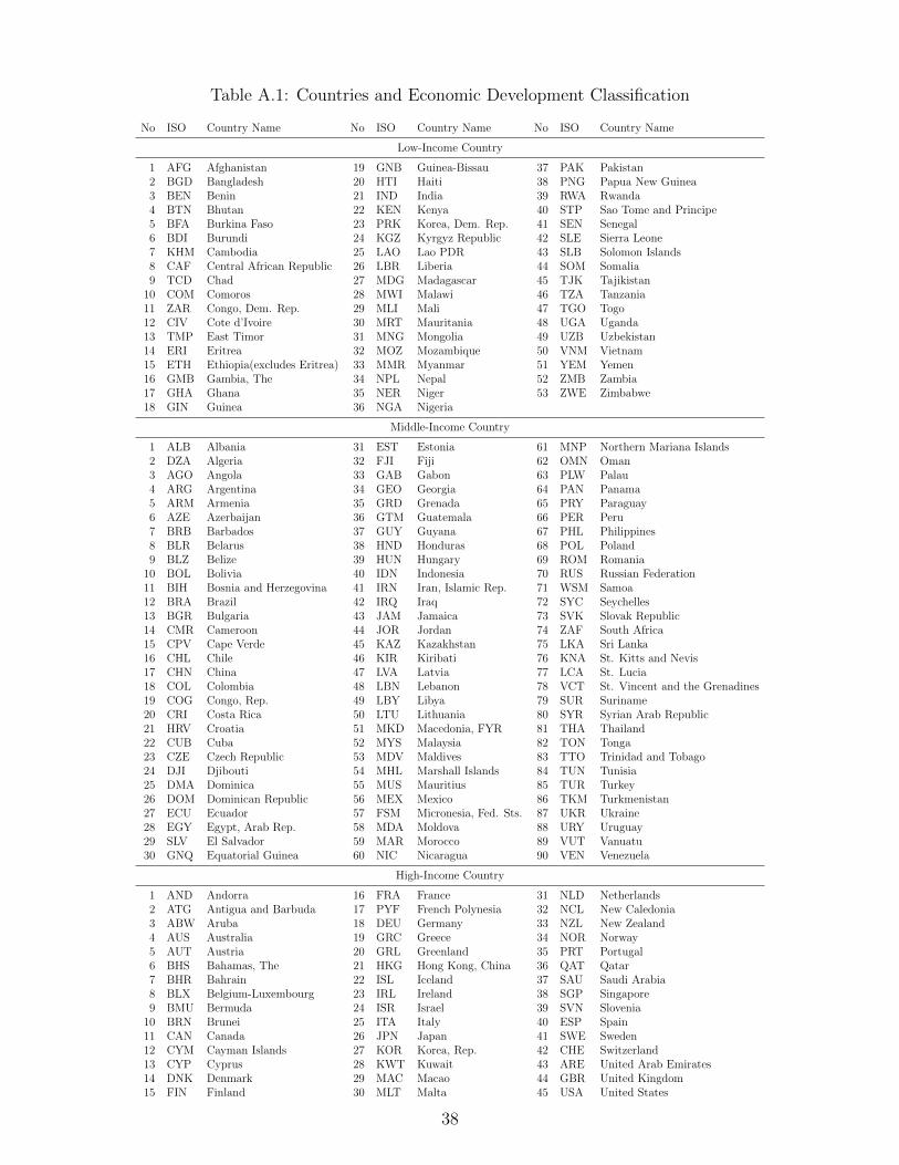
Table A.1: Countries and Economic Development Classification
No ISO Country Name No ISO Country Name No ISO Country Name
Low-Income Country
1 AFG Afghanistan 19 GNB Guinea-Bissau 37 PAK Pakistan2 BGD Bangladesh 20 HTI Haiti 38 PNG Papua New Guinea3 BEN Benin 21 IND India 39 RWA Rwanda4 BTN Bhutan 22 KEN Kenya 40 STP Sao Tome and Principe5 BFA Burkina Faso 23 PRK Korea, Dem. Rep. 41 SEN Senegal6 BDI Burundi 24 KGZ Kyrgyz Republic 42 SLE Sierra Leone7 KHM Cambodia 25 LAO Lao PDR 43 SLB Solomon Islands8 CAF Central African Republic 26 LBR Liberia 44 SOM Somalia9 TCD Chad 27 MDG Madagascar 45 TJK Tajikistan
10 COM Comoros 28 MWI Malawi 46 TZA Tanzania11 ZAR Congo, Dem. Rep. 29 MLI Mali 47 TGO Togo12 CIV Cote d’Ivoire 30 MRT Mauritania 48 UGA Uganda13 TMP East Timor 31 MNG Mongolia 49 UZB Uzbekistan14 ERI Eritrea 32 MOZ Mozambique 50 VNM Vietnam15 ETH Ethiopia(excludes Eritrea) 33 MMR Myanmar 51 YEM Yemen16 GMB Gambia, The 34 NPL Nepal 52 ZMB Zambia17 GHA Ghana 35 NER Niger 53 ZWE Zimbabwe18 GIN Guinea 36 NGA Nigeria
Middle-Income Country
1 ALB Albania 31 EST Estonia 61 MNP Northern Mariana Islands2 DZA Algeria 32 FJI Fiji 62 OMN Oman3 AGO Angola 33 GAB Gabon 63 PLW Palau4 ARG Argentina 34 GEO Georgia 64 PAN Panama5 ARM Armenia 35 GRD Grenada 65 PRY Paraguay6 AZE Azerbaijan 36 GTM Guatemala 66 PER Peru7 BRB Barbados 37 GUY Guyana 67 PHL Philippines8 BLR Belarus 38 HND Honduras 68 POL Poland9 BLZ Belize 39 HUN Hungary 69 ROM Romania
10 BOL Bolivia 40 IDN Indonesia 70 RUS Russian Federation11 BIH Bosnia and Herzegovina 41 IRN Iran, Islamic Rep. 71 WSM Samoa12 BRA Brazil 42 IRQ Iraq 72 SYC Seychelles13 BGR Bulgaria 43 JAM Jamaica 73 SVK Slovak Republic14 CMR Cameroon 44 JOR Jordan 74 ZAF South Africa15 CPV Cape Verde 45 KAZ Kazakhstan 75 LKA Sri Lanka16 CHL Chile 46 KIR Kiribati 76 KNA St. Kitts and Nevis17 CHN China 47 LVA Latvia 77 LCA St. Lucia18 COL Colombia 48 LBN Lebanon 78 VCT St. Vincent and the Grenadines19 COG Congo, Rep. 49 LBY Libya 79 SUR Suriname20 CRI Costa Rica 50 LTU Lithuania 80 SYR Syrian Arab Republic21 HRV Croatia 51 MKD Macedonia, FYR 81 THA Thailand22 CUB Cuba 52 MYS Malaysia 82 TON Tonga23 CZE Czech Republic 53 MDV Maldives 83 TTO Trinidad and Tobago24 DJI Djibouti 54 MHL Marshall Islands 84 TUN Tunisia25 DMA Dominica 55 MUS Mauritius 85 TUR Turkey26 DOM Dominican Republic 56 MEX Mexico 86 TKM Turkmenistan27 ECU Ecuador 57 FSM Micronesia, Fed. Sts. 87 UKR Ukraine28 EGY Egypt, Arab Rep. 58 MDA Moldova 88 URY Uruguay29 SLV El Salvador 59 MAR Morocco 89 VUT Vanuatu30 GNQ Equatorial Guinea 60 NIC Nicaragua 90 VEN Venezuela
High-Income Country
1 AND Andorra 16 FRA France 31 NLD Netherlands2 ATG Antigua and Barbuda 17 PYF French Polynesia 32 NCL New Caledonia3 ABW Aruba 18 DEU Germany 33 NZL New Zealand4 AUS Australia 19 GRC Greece 34 NOR Norway5 AUT Austria 20 GRL Greenland 35 PRT Portugal6 BHS Bahamas, The 21 HKG Hong Kong, China 36 QAT Qatar7 BHR Bahrain 22 ISL Iceland 37 SAU Saudi Arabia8 BLX Belgium-Luxembourg 23 IRL Ireland 38 SGP Singapore9 BMU Bermuda 24 ISR Israel 39 SVN Slovenia
10 BRN Brunei 25 ITA Italy 40 ESP Spain11 CAN Canada 26 JPN Japan 41 SWE Sweden12 CYM Cayman Islands 27 KOR Korea, Rep. 42 CHE Switzerland13 CYP Cyprus 28 KWT Kuwait 43 ARE United Arab Emirates14 DNK Denmark 29 MAC Macao 44 GBR United Kingdom15 FIN Finland 30 MLT Malta 45 USA United States
38