Exporting Behavior of Foreign A¢ liates:Theory and Evidence�

Jiangyong Lua, Yi Lub, and Zhigang Taoba Peking University

b University of Hong Kong

March 2010

Abstract

Firms have increasingly conducted di¤erent stages of production indi¤erent countries. In particular, they may set up operations in low-cost countries (those operations are referred to as foreign a¢ liates inthose countries) either as platforms for export or serving the growingmarkets there. What is the exporting behavior of foreign a¢ liates? Inthis paper, using data from China, we �nd that among foreign a¢ li-ates exporters are less productive than non-exporters. We then o¤era theoretical explanation by incorporating into the standard �rm het-erogeneity model the possibility that �rms could have di¤erent stagesof production in di¤erent countries.

Keywords: Foreign A¢ liates, Exporting Behavior, Firm Hetero-geneityJEL Codes: F12, F23, L22, D24, L60

�We would to thank a co-editor and two anonymous referees for valuable comments andsuggestions, and Linhui Yu for expert research assistance. The �rst author acknowledges�nancial support from National Natural Science Foundation of China (70703017) andGuanghua Leadership Institute in Collaboration with Cisco, and the other two authorsthank Hong Kong Research Grants Council and University of Hong Kong for �nancialsupport.

1

1 Introduction

Since mid-1990s, there has been increasing evidence suggesting that export-ing behavior varies signi�cantly across �rms even after controlling for indus-try e¤ects (see, for example, Bernard and Jensen, 1995, 1999). A unanimous�nding in the literature is that exporters are more productive than non-exporters (called export premium), e.g., Bernard and Jensen (1995, 1999,2004) for the study of the United States; Bernard and Wagner (1997) forthe study of Germany; Clerides, Lach, and Tybout (1998) for the study ofColumbia, Mexico and Morocco; and Greenaway and Kneller (2004) for thestudy of the United Kingdom. A dominant theoretical explanation for theexport premium result is based on the existence of �xed costs of export-ing, under which more productive �rms self-select to become exporters (e.g.,Bernard, Eaton, Jensen, and Kortum, 2003; Melitz, 2003; and Bernard, Red-ding, and Schott, 2007).1

However, almost all the existing studies implicitly focus on the exportingbehavior of domestic �rms, or at least they do not explicitly di¤erentiate do-mestic �rms from foreign a¢ liates (foreign-invested �rms operating in thosecountries).2 As transport and communications costs decrease, �rms haveincreasingly conducted di¤erent stages of production in di¤erent countries.In particular, �rms may set up their production plants in low-cost countriessuch as Brazil, China, India, and Russia as their export platforms, whichis referred to as vertical foreign direct investment (or FDI) in the literature(e.g., Hummels, Ishii, and Yi, 2001; Yeaple, 2003; Yi, 2003; Grossman, Help-man, and Szeidl, 2006; Ekholm, Forslid, and Markusen, 2007).3 As a result, asigni�cant percentage of export from those low-cost countries is made by for-eign a¢ liates in the countries. Is the exporting behavior of foreign a¢ liatessimilar to that of domestic �rms? In this paper, we �ll the void by investi-gating empirically the exporting behavior of foreign a¢ liates using data fromChina, and then o¤er a theoretical explanation for the empirical �ndings.4

1Some recent studies, however, show that there also exists learning from exporting(e.g., Blalock and Gertler, 2004; Van Biesebroeck, 2005; De Loecker, 2007).

2Baldwin and Gu (2003) and Kneller and Pisu (2004) are two exceptions, using datafrom Canada and UK respectively, but neither has found any signi�cant di¤erence betweendomestic �rms and foreign a¢ liates. Presumably, the sample sizes of foreign a¢ liates inthese two countries are not large enough.

3It should be pointed out that foreign multinationals may also have direct investmentin those countries to serve the growing markets there, and such investment is referred toas horizontal FDI in the literature (Markusen, 2002).

4Here exporting behavior refers to how foreign a¢ liates with di¤erent productivitychoose to set up di¤erent stages of production in di¤erent countries and the associatedexport status.

2

China o¤ers an ideal setting to investigate this issue. Between 1979 and2005, China has attracted more than US$1,285 billion FDI (China StatisticalYearbook, 2006). Meanwhile, China was the second largest exporter in theworld in 2007 (The World Factbook, 2007). More importantly, much ofChina�s export has been made by foreign a¢ liates, not China�s domestic�rms (Manova and Zhang, 2008).Our dataset comes from annual surveys of manufacturing �rms conducted

by the National Bureau of Statistics of China for the period of 1998 to 2005.We �nd that among China�s domestic �rms, exporters are indeed more pro-ductive than non-exporters, similar to the unanimous �nding in the existingliterature. Surprisingly, for foreign a¢ liates in China, exporters are foundto be less productive. Moreover, we �nd that, among foreign a¢ liates, thoseselling all their output in China have the highest productivity, followed bythose having sales in China and also exporting some of their output, and�nally those exporting all their output. These �ndings remain robust to anumber of sensitivity checks, such as an alternative measure of productivity,an alternative estimation method, an alternative de�nition of foreign a¢ li-ates, exclusion of outlying observations, inclusion of �rm size as an additionalcontrol variable, and estimation of productivity separately for domestic �rmsand foreign a¢ liates.We next construct a simple model to explain the exporting behavior of

foreign a¢ liates. It is a standard 2� 2� 2 trade model à la Grossman, Help-man, and Szeidl (2006), with two sectors (i.e., homogenous good sector anddi¤erentiated goods sector), two factors (i.e., skilled labor and unskilled la-bor), and two countries (i.e., China and the United States). Similar to Melitz(2003)�s setting, �rms di¤er in their productivity, which is drawn from a com-mon distribution. There are two vertically-related stages of the productionprocess, i.e., design and manufacturing. The United States has a cost advan-tage in design whereas China has a cost advantage in manufacturing. Forsimplicity, we assume there is a negligible transport cost for shipping the de-sign product to the manufacturing plant, thereby the design stage is alwayslocated in the United States. But the transport cost for shipping the �nalproduct to an abroad market is non-trivial, thereby �rms can choose to setup their manufacturing plant in either the United States, or China, or both.Firms can also choose to sell their output in the United States, or China,or both. There is a �xed cost for setting up a manufacturing plant in anyof these two countries, and also a �xed cost of selling in any of these twomarkets.Under this framework, there are nine possible strategies in organization

choice and market orientation, i.e., manufacturing plant in either the UnitedStates, or China, or both, and selling in either the United States, or China, or

3

both. We can show that in equilibrium there are four strategies correspond-ing to the three types of foreign a¢ liates observed in our dataset: foreigna¢ liates selling all their output in China, those exporting all their output,and those having sales in China and exporting some of their output. Thecomparison among these four strategies in terms of their productivity o¤ersan explanation for the puzzling exporting behavior of foreign a¢ liates (i.e.,exporters have lower productivity than non-exporters among foreign a¢ li-ates).5 Intuitively, the choice among the di¤erent strategies depends on thetrade-o¤ between �xed costs and production e¢ ciency (determined by thesize of the markets and the unit cost of production). Compare, for example,the strategy of exporting all their output with the strategy of having salesin China and exporting some of their output. The latter strategy gains anextra market (i.e., the market in China) but needs to incur a �xed cost ofselling in China. Clearly the more productive foreign a¢ liates choose thelatter strategy given the trade-o¤ between �xed costs and market size.Our paper builds upon a large literature of �rm heterogeneity and trade.

What di¤erentiates our paper from the literature is its focus on the export-ing behavior of foreign a¢ liates, which are increasingly prevalent in today�sglobal economy. We show that the relation between productivity and ex-porting behavior for foreign a¢ liates is just the opposite of the unanimous�nding in the literature which focuses on domestic �rms. Theoretically, byincorporating into the standard �rm heterogeneity model (Melitz, 2003) thepossibility that �rms could set up di¤erent stages of production in di¤erentcountries à la Grossman, Helpman, and Szeidl (2006), we are able to ob-tain richer predictions on the relation between productivity and exportingbehavior.The remainder of the paper is structured as follows. Section 2 describes

data, and Section 3 presents our empirical �ndings. In Section 4, we o¤era theoretical model to explain our empirical �ndings. The paper concludeswith Section 5.

2 Data and Descriptive Statistics

Our data is from annual surveys of manufacturing �rms conducted by theNational Bureau of Statistics of China for the period of 1998 to 2005. Theseannual surveys covered all state-owned enterprises, and those non-state-owned enterprises with annual sales of �ve million Chinese currency (about

5Our framework can also show that, for domestic �rms in China, it is the more pro-ductive ones that export, which is consistent with our empirical �ndings and in line withthe predictions of other theoretical models in the literature.

4

US$650,000) or more. The data provides detailed information on �rms�iden-ti�cation, operations and performance, including �rm ownership and export,which are of special interest to this study. As reported in Table 1a, thenumber of manufacturing �rms with valid information of total output andexport varies from over 140,000 in the late 1990s to over 243,000 in 2005.The percentage of China�s total exports contributed by �rms in our datasetwas just below 70% in late 1990s, and was as high as 76% in 2005, indicatingthat our data set is highly comprehensive.The focus of this study is on the exporting behavior of foreign a¢ liates.

According to the classi�cation of the National Bureau of Statistics of China,foreign a¢ liates are �rms in which 25% or more equity shares are held byforeign multinationals.6 We use this de�nition of foreign a¢ liates in mostof our analysis. As a robustness check, we also use �rm�s ownership typereported in the dataset to de�ne foreign a¢ liates. Speci�cally, there are �vetypes of ownership: state-owned �rms, collectively-owned �rms, joint-stockcompanies, privately-owned �rms, and foreign-invested �rms. We treat �rmswith foreign-invested ownership type as foreign a¢ liates.As shown in Table 1b, over the period of 1998 to 2005, an average of

27.14% of China�s manufacturing �rms (including both domestic �rms andforeign a¢ liates) exported. Foreign a¢ liates are much more export-orientedthan do domestic �rms: 62.95% of foreign a¢ liates are exporters whereas thecorresponding number for domestic �rms is 18.68%. The di¤erence betweenthese two types of �rms in export intensity is even greater: the percentage ofexport in total output hovered around 10.48% for China�s domestic �rms overthe sample period, whereas that for foreign a¢ liates increased from 39.23%in 1998 to 44.60% in 2005.7 Taken together, the percentage of China�s totalexport by foreign a¢ liates increased from 59.66% in 1998 to 70.98% in 2005,showing that foreign a¢ liates are the main driver behind the spectacular riseof China�s export.Exporting behavior of China�s manufacturing �rms varies signi�cantly

across its geographic areas.8 As shown in Table 1c, foreign a¢ liates located

6Our main results remain robust if �rms from Hong Kong, Macau and Taiwan areexcluded from the sample.

7From the 2002 U.S. census of manufacturers, it is found that 20% of U.S. manufac-turing plants exported and the exporters shipped 15% of their output abroad (Bernard,Jensen, Redding, and Schott, 2007). The percentage of exporters in the French manufac-turing industries is also 20%, though the export intensity is lower at 10% (Eaton, Kortumand Kramarz, 2004).

8During the sample period, China�s administrative boundaries and consequently itscounty, city, or even provincial codes experienced some changes. For example, new countieswere established, while existing counties were combined into larger ones or even elevated tocities. From 1998 to 2005, the number of counties in China increased from 2,496 to 2,862 (a

5

in China�s coastal area have higher propensities to export and higher exportintensities than those located in China�s central area, which in turn havehigher propensities to export and higher export intensities than those lo-cated in China�s western area. Presumably, foreign a¢ liates located in thecentral and western areas focus more on China�s domestic markets than theircounterparts located in the coastal area. Meanwhile, China�s domestic �rmshave lower propensities to export and lower export intensities than foreigna¢ liates in each of the three areas. There is little di¤erence in the propen-sity to export between domestic �rms located in the coastal area and thosein the central area, though the former have much higher export intensitythan the latter. Overall, 93.8% percent of China�s total exports are made by�rms located in the coastal area, and 71.4% of these exports are from foreigna¢ liates in this area.Besides the di¤erences across geographic areas, there are also signi�cant

variations in exporting behavior across industries.9 As the technology contentof China�s exports has become an interesting topic, we look at the patternsof exporting behavior across the low-tech, medium-tech, and high-tech in-dustries classi�ed according to the OECD standard. Several patterns emergefrom the results summarized in Table 1d: (1) 51.8% of China�s export isfrom the high-tech industries, followed by 32.0% in the low-tech industriesand 16.2% in the medium-tech industries. Given China�s comparative ad-vantage in low-tech industries, it seems puzzling that China exports largeamounts of high-tech goods as well as low-tech goods (Rodrik, 2006; Wangand Wei, 2008; Lu and Xu, 2009). (2) In the high-tech industries and low-tech industries, compared with the national averages, both foreign a¢ liatesand domestic �rms have higher propensities to export and higher export in-tensities, accounting for the high export in these two types of industries.

total of 366), while the number of changes in the county codes was 648. From 1998 to 2005,the number of prefecture-level cities or above increased from 231 (4 municipalities, 15 viceprovincial cities, and 212 prefecture-level cities) to 287 (4 municipalities, 15 vice provincialcities, and 268 prefecture-level cities). Using the 1999 National Standard (promulgatedat the end of 1998 and called GB/T 2260-1999) as the benchmark codes, we convert theregional codes of all the �rms to these benchmark codes to achieve consistency for theregional codes in the whole sample period.

9In 2003, a new classi�cation system for industry codes (called GB/T 4754-2002) wasadopted to replace the old classi�cation system (called GB/T 4754-1994) that had beenused from 1995 to 2002. To achieve consistency in the industry codes for the wholesample period (1998-2005), we convert the industry codes in the 2003-2005 data to theold classi�cation system by using a concordance table (in the case of a new four-digitcode corresponding to an old four-digit code or several new four-digit codes correspondingto an old four-digit code) or by assigning a new code for an old code based on productinformation (in the case of several old four-digit codes corresponding to a new 4-digitcode).

6

(3) Foreign a¢ liates are responsible for 82.8% percentage of export in thehigh-tech industries, indicating that much of the worry about the increasingcompetitiveness of China�s exports in the high-tech industries might well bemisguided as export in the high-tech industries are made by foreign a¢ liatesrather than China�s domestic �rms.Table 1e provides further descriptive statistics regarding the exporting

behavior of foreign a¢ liates, which is the focus of this paper. Over theperiod of 1998-2005, on average, 37.05% of foreign a¢ liates sell all theiroutput in China, 39.22% of foreign a¢ liates have sales in China and alsoexport some of their output, and 23.73% of foreign a¢ liates export all theiroutput. Meanwhile, during this period, the percentage of foreign a¢ liateshaving both sales in China and export increases at the expenses of foreigna¢ liates selling all their output in China and those exporting all their output.

3 Empirical Analysis

In this section, we empirically investigate the exporting behavior of foreigna¢ liates in China. The key performance indicator used in the literature todocument the possible di¤erence between exporters and non-exporters is thetotal factor productivity (TFP), e.g., Bernard and Jensen (1995, 1999, 2004),Bernard and Wagner (1997), Clerides, Lach, and Tybout (1998), Greenawayand Kneller (2004), and De Loecker (2007). Speci�cally, we estimate thefollowing equation:

TFPfirt = �+ � � Exportfirt + �i + �r + �t + "firt (1)

where TFPfirt is the TFP of �rm f in industry i, region r and year t;Exportfirt is a dummy variable indicating whether �rm f is an exporter;�i, �r and �t are 4-digit industry dummy, region dummy,

10 and year dummy,respectively; and "firt is the error term.Four variables are used to estimate TFP: output, labor, capital, and

intermediate inputs. After deleting observations with missing informationrelated to these four variables, we obtain a balanced sample of 31,057 �rmsthat appeared in the dataset for all eight years from 1998 to 2005. Anadditional 51 �rms are deleted because of missing information about export.As the focus of our study is on the exporting behavior of foreign a¢ liates, wefurther exclude �rms that switched, one time or more, from foreign a¢ liatesto domestic �rms, or vice versa. Speci�cally, a total of 3,158 �rms are deleted

10Region here refers to 22 provinces, 4 province-level municipalities, and 5 minorityautonomous regions in China.

7

when foreign a¢ liates are de�ned as �rms with 25% or more equity sharesheld by foreign multinationals, whereas a total of 1,104 �rms are deletedwhen foreign a¢ liates are de�ned by their reported ownership type.We �rst use the ordinary-least-squares (OLS) regression method to es-

timate the TFP for �rms in each 2-digit industry and each year (denotedby TFP OLS) (see also Bernard and Jensen, 1999). Speci�cally, we usethe constant value of output, and de�ate capital by the �xed-assets invest-ment price index and intermediate inputs by the producer price index. TheOLS estimation of TFP, however, may su¤er from the simultaneity problem,speci�cally, input choices could be endogenously determined by unobserv-able productivity shocks. This may lead to an upward bias in the estimationcoe¢ cients of more variable inputs such as labor (Van Biesebroeck, 2007,2008).We therefore use an alternative estimation method, i.e., Levinsohn and

Petrin (2003)�s TFP estimation method (denoted by TFP LP ), in whichthe intermediate inputs are used as a proxy for unobservable productivityshocks to deal with the simultaneity problem.11 As Levinsohn and Petrin(2003)�s TFP estimation method relies on the panel estimation of �rms thatremain in the same industries throughout the estimation period, we thereforedelete those �rms that experienced changes in their 2-digit industry a¢ lia-tions during the sample period. We end up with a reduced sample of 22,549�rms. The average coe¢ cients for labor, capital and intermediate inputs are0.055, 0.032 and 0.743 respectively (the estimated coe¢ cients of inputs foreach 2-digit industry are available online). For comparison, we also use theOLS method to estimate TFP for this reduced sample in each 2-digit indus-try and each year (denoted by TFP OLSR) (results are available online).The average coe¢ cients for labor, capital and intermediate inputs under theOLS estimation are 0.062, 0.036 and 0.891 respectively. Consistent with the�ndings in Levinsohn and Petrin (2003) and Van Biesebroeck (2008), thecoe¢ cient for labor is over-estimated under the OLS method.Moreover, as a further robustness check, we re-estimate the TFP at more

disaggregated industry level. Speci�cally, we use the OLS method to estimatethe TFP in each 3-digit industry and each year (denoted by TFP OLS3D),and the Levinsohn and Petrin (2003)�s method in each 3-digit industry (de-noted by TFP LP 3D).12

11An alternative method for dealing with the endogeneity problem is Olley and Pakesmethod (1996), which uses investment as a proxy for unobservable productivity shocks.However, there is a large number of missing information on investment in our dataset(i.e, only 5,943 �rms out of 27,848 have positive investment). Therefore Olley and Pakesmethod is not econometrically e¢ cient in our case.12In the OLS estimation, as some industry-year cells have very few observations, we

8

Benchmark regression results for equation (1) are reported in Table 2. Asshown in Column 1, when all �rms are included in the regression analysis,Exportfirt has a positive and statistically signi�cant e¤ect on TFP estimatedusing the OLS method, which is similar to the �ndings reported in the lit-erature. Next, we carry out the analysis for the two sub-samples, one fordomestic �rms and the other for foreign a¢ liates, and report the resultsin Columns 2-3 of Table 2, respectively. Surprisingly, we �nd contrastingpatterns of exporting behavior between domestic �rms and foreign a¢ liates.The estimated coe¢ cient of Exportfirt for foreign a¢ liates becomes negativeand statistically signi�cant, though that for domestic �rms remains positiveand statistically signi�cant. The negative coe¢ cient of Exportfirt for foreigna¢ liates remains robust when the TFP is estimated using Levinsohn andPetrin (2003)�s method (Column 4 of Table 2); when the TFP is estimatedusing the OLS method for the same reduced sample as used in the Levinsohnand Petrin (2003)�s estimation (Column 5 of Table 2); and when the TFP isestimated using the OLS and the Levinsohn and Petrin (2003)�s method atthe 3-digit industry level (Columns 6-7 of Table 2).As there are three types of foreign a¢ liates (i.e., foreign a¢ liates with

domestic sales only, those with both domestic sales and export, and thosewith export only), we therefore replace the export dummy of equation (1)by two dummy variables: one for foreign a¢ liates with domestic sales only(denoted by Domestic Sales Onlyfirt), and the other for foreign a¢ liateswith export only (denoted by Export Onlyfirt). As shown in Columns 8-12of Table 2, the coe¢ cients for Domestic Sales Onlyfirt are positive albeitstatistically insigni�cant when the TFP is estimated using the OLS method,but they are both positive and statistically signi�cant when the TFP is es-timated using the Levinsohn and Petrin (2003)�s method. Meanwhile, thecoe¢ cients for Export Onlyfirt are always negative and statistically signi�-cant. These results o¤er a �ner ranking of foreign a¢ liates in terms of theirproductivity. Speci�cally, foreign a¢ liates with domestic sales only have thehighest productivity, followed by those with both domestic sales and export,and �nally those with export only.13

Note that our analysis thus far is based on the balanced sample of �rms forthe period of 1998-2005. As China continues its rapid economic growth, there

exclude those cells with observations below 10 to reduce possible estimation biases. Inthe Levinsohn and Petrin (2003)�s estimation, we exclude those �rms that changed their3-digit industry a¢ liations during the sample period.13The ranking of the average TFP (estimated using Levinsohn and Petrin (2003)�s

method) among these three types of foreign a¢ liates in each of the twenty-eight two-digitmanufacturing industries is in general consistent with our regression results (availableonline).

9

has been a surge of foreign direct investment aiming at capturing the Chinesemarket in more recent years. Thus it would be interesting to investigateif newly established foreign a¢ liates behave di¤erently from those in thebalanced sample. We then use the full sample of �rms in 2005, and reportthe regression results in Table 3. It is found that the coe¢ cient of dummyvariable Export Onlyfirt remains negative albeit statistically insigni�cant(Column 1 of Table 3), generally consistent with our results in Table 2. InColumn 2, we replace the dummy variable Export Onlyfirt by two otherdummy variables (Domestic Sales Onlyfirt, and Export Onlyfirt), and �ndthat the coe¢ cients of these two dummy variables are both negative andstatistically signi�cant. These results imply that foreign a¢ liates exportingall their output are less productive than those having both sales in Chinaand exporting some of their output (consistent with our results in Table 2),but that foreign a¢ liates selling all output in China become less productivethan those having both sales in China and exporting some of their output(in contrast with those in Table 2). As our theoretical analysis will show,there are two types of foreign a¢ liates selling all their output in China, onefocuses exclusively on the Chinese market and the other has presence in bothChinese and world markets. The contrasting �nding between Table 2 andTable 3 can be explained as that foreign a¢ liates entering into China after1998 may predominantly focus exclusively on the growing market in China,thereby overshadowing those older foreign a¢ liates having presence in boththe Chinese and world markets.In the remaining part of this section, we conduct a series of robustness

checks regarding the relation between �rm productivity and exporting behav-ior for foreign a¢ liates. To save space, we only report the results using theTFP estimated by Levinsohn and Petrin (2003)�s method as the dependentvariable and using the balanced sample for the period 1998-2005.First, we use an alternative de�nition of foreign a¢ liates � the o¢ cial

ownership type reported by the �rm in the survey �instead of that impliedby foreign equity ownership. As shown in Column 1 of Table 4, our mainresults remain robust to this de�nition of foreign a¢ liates.Second, to address the concern that our results could be driven by some

outlying observations, we exclude the top and bottom 1% observations in oursample and repeat the analysis. As shown in Column 2 of Table 4, our mainresults remain robust to the exclusion of outlying observations.Third, to make sure that our results are not entirely driven by �rm size, we

incorporate Firm Size (de�ned as the logarithm of capital) in the regressionanalysis. The result reported in Column 3 of Table 4 reveal that our �ndingsremain robust to the inclusion of Firm Size.Lastly, to deal with the concern that foreign a¢ liates may have di¤erent

10

production functions from domestic �rms, we re-estimate the TFP of foreigna¢ liates using only the sub-sample of foreign a¢ liates. As shown in Column4 of Table 4, our main �ndings remain robust to this alternative estimationof TFP.Taken together, the empirical analysis in this section shows that for for-

eign a¢ liates, those exporting all their output are less productive than thosehaving both sales in China and also exporting some of their output, whichin turn are generally less productive than those selling all their output inChina. To the best of our knowledge, this is the �rst study reporting thatexporters are less productive than non-exporters in the literature. Our studyis also one of the few studies on the exporting behavior of foreign a¢ liates.

4 Theoretical Analysis

In this section, we build a simple model based on Grossman, Helpman, andSzeidl (2006) to explain our empirical �ndings regarding the exporting be-havior of foreign a¢ liates documented in the previous section.

4.1 Model Setup

It is a standard 2 � 2 � 2 trade model, in which there are two countries(i.e., China (C) and the United States (A)), two sectors (i.e., a homogeneousgood (X) produced with a constant return to scale technology and a contin-uum of di¤erentiated goods (Y ) produced with an increasing return to scaletechnology), and two factors (i.e., skilled labor and unskilled labor).Following the literature (i.e., Dixit and Stiglitz, 1977), we take the ho-

mogeneous good (X) as a numéraire and assume the utility function for thedi¤erentiated goods (Y ) to be a constant elasticity of substitution function.Then the demand function for any di¤erentiated good in country l can bederived as:

yl = ���1�� I l(pl)

�11�� ; 0 < � < 1 (2)

where l 2 fA;Cg is the index for the country; yl is the consumption of thedi¤erentiated good in country l; I l is the aggregate demand level (or marketsize) in country l; and pl is the price of the di¤erentiated good in country l.There are two vertically-related stages for producing any variety of the

di¤erentiated goods, i.e., design (d) and manufacturing (m). It is assumedthat the design stage is more intensive in the usage of skilled labor than doesthe manufacturing stage, and that the United States has a lower wage ofskilled labor but a higher wage of unskilled labor than does China. Thus

11

the United States has a cost-advantage in design while China has a cost-advantage in manufacturing, i.e., the design cost in the United States (dA)is lower than that in China (dC), but the manufacturing cost in the UnitedStates (mA) in higher than that in China (mC). The unit cost for producingthe �nal product is then given by c(dl;ml)=�, where the �rst term of c(:; :)indicating the design cost and the second term indicating the manufacturingcost, and � is the �rm-speci�c productivity measure, which is drawn from acommon distribution as in Melitz (2003).There is a �xed cost associated with setting up a plant of design or man-

ufacturing in any of the two countries. We assume that the �xed cost usesthe same intensity of skilled labor and unskilled labor as the unit produc-tion cost (for the use of same assumption, see for example Baldwin, Forslid,Martin, Ottaviano, and Robert-Nicoud, 2003; Bernard, Redding, and Schott,2007). Thus the �xed cost of setting up a design plant in the United States(fAd ) is lower than that in China (f

Cd ) whereas the �xed cost of setting up a

manufacturing plant in the United States (fAm) in higher than that in China(fCm).There is also a �xed cost involved with the sales of the �nal product, e.g.,

the costs of setting up a distribution network. To take into account of thepossible heterogeneity in selling costs, we assume that the �xed cost of sellingthe di¤erentiated good in any of the two countries is fs if the manufacturingof the �nal product takes place in the same country, but is increased tofs +�fs if the manufacturing takes place in a di¤erent country.It is assumed that the transport cost for the design product is negligible

(e.g., the design product could be transmitted by E-mail or sent by expressmail), but there is a non-zero transport cost for shipping the �nal productto an abroad market. Speci�cally, the transport cost takes the form of aniceberg cost, i.e., one needs t > 1 units of �nal product in order to ship 1unit to an abroad market. It is further assumed that the transport cost forthe �nal product is non-trivial, i.e., for the market in the United States, theunit cost for the �nal product is higher when the �nal product is importedfrom China than when it is produced in the United States (called the tari¤-jumping assumption). Without this assumption, manufacturing is alwaysconducted in China, which makes the analysis less interesting.14

A �rm needs to make two decisions, one is where to set up its designand manufacturing plants and the other is where to sell its �nal product.As there is a negligible transport cost for the design product and the United

14More generally, if this assumption is not satis�ed, production processes are completelydisintegrated with each production stage located in the country with the comparativeadvantage.

12

States has cost-advantages in both the �xed cost and the unit productioncost for the design stage, the design plant is always located in the UnitedStates.15 However, for the manufacturing plant, it could be located in theUnited States only (A), China only (C), or both the United States and China(AC). Meanwhile, a �rm can sell its �nal product in the United States only(A), China only (C), or both the United States and China (AC).Let �(:; :; :) denote a strategy for the �rm, where the �rst entry represents

the location of the design plant, the second entry represents the location ofthe manufacturing plant, and the last entry represents the location of the �nalproduct market. There are altogether nine possible strategies: �(A;A;A),�(A;A;C), �(A;A;AC), �(A;C;A), �(A;C;C), �(A;C;AC), �(A;AC;A),�(A;AC;C), and �(A;AC;AC).

4.2 Equilibrium Strategy

Given the above setup, we can derive the equilibrium pro�t function for eachpossible strategy (�(�)). In analyzing the optimal strategy, we adopt theiterated elimination method, i.e., once a possible strategy is dominated byanother, it is eliminated from the choice.Step 1: �(A;A;C), �(A;AC;A), and �(A;AC;C) are dominated strate-

gies.�(A;A;C) (design and manufacturing in the United States, and selling

in China) is dominated by �(A;C;C) (design in the United States, and man-ufacturing and selling in China), because the latter enjoys a lower manu-facturing cost and does not need to incur any transport cost for the �nalproduct.�(A;AC;A) (design in the United States, manufacturing in both the

United States and China, and selling in the United States) is dominated byeither �(A;A;A) (design, manufacturing and selling in the United States).Because of the tari¤-jumping assumption, the market in the United States isonly served by the manufacturing plant in the United States. As a result, theformer strategy incurs a redundant �xed cost of setting up a manufacturingplant in China.�(A;AC;C) (design in the United States, manufacturing in both the

United States and China, and selling in China) is dominated by �(A;C;C)(design in the United States, and manufacturing and selling in China). Inthis case, the market in China is only served by the manufacturing plant

15It is commonly assumed in the literature that the design stage is always located inthe United States and �rms only decide where to set up their manufacturing plants, e.g.,Antras (2003), Antras and Helpman (2004), and Helpman and Grossman (2005).

13

in China due to the lower manufacturing cost in China and the saving oftransport costs. As a result, the former strategy incurs a redundant �xedcost of setting up a manufacturing plant in the United States.Step 2: �(A;A;A) and �(A;A;AC) are not observed in our dataset.Both �(A;A;A) (design, manufacturing and selling in the United States)

and �(A;A;AC) (design and manufacturing in the United States, and sellingin both the United States and China) represent the American domestic �rmsas all their production takes place in the United States. In the �rst case, the�rm sells all its output in the United States, and in the second case the �rmexports some of its output to China (to China it is import). Thus, these twocases are not foreign a¢ liates in China and not observed in our dataset.Step 3: the comparison among �(A;C;C), �(A;C;A), �(A;C;AC), and

�(A;AC;AC).Now we are left with only four possible strategies: �(A;C;C) represents

the strategy with design in the United States, manufacturing in China, andselling in China; �(A;C;A) represents the strategy with design in the UnitedStates, manufacturing in China, and selling in the United States; �(A;C;AC)is the strategy with design in the United States, manufacturing in China,and selling in both the United States and China; and �(A;AC;AC) is thestrategy with design in the United States, manufacturing and selling in boththe United States and China (and due to the tari¤-jumping assumption, themanufacturing plant in the United States serves only the market there whilethe manufacturing plant in China serves only the Chinese market).The pro�t functions for foreign a¢ liates adopting these four strategies

can be shown as follows:8>>>>>><>>>>>>:

�(�(A;C;C)) = (1��)ICC(dA;mC)

�� (fAd + fCm + fs)

�(�(A;C;A)) =(1��) I

A

T

C(dA;mC)�� (fAd + fCm + fs +�fs)

�(�(A;C;AC)) =(1��)

�IC+ IA

T

�C(dA;mC)

�� (fAd + fCm + 2fs +�fs)�(�(A;AC;AC)) =

�(1��)ICC(dA;mC)

+ (1��)IAC(dA;mA)

��� (fAd + fAm + fCm + 2fs)

;

(3)where � � �

�1�� is a monotonic transform of productivity �; C(:; :) �

c (:; :)�

1�� is a monotonic transform of unit production cost c (:; :); T � t�

1��

is a monotonic transform of transport cost t; and I l is the market size incountry l, l 2 fA;Cg.It is clear that the pro�t function for each of these four strategies is a

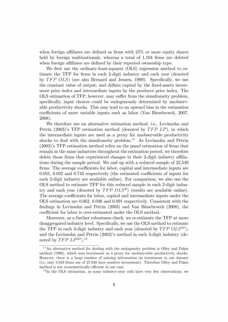
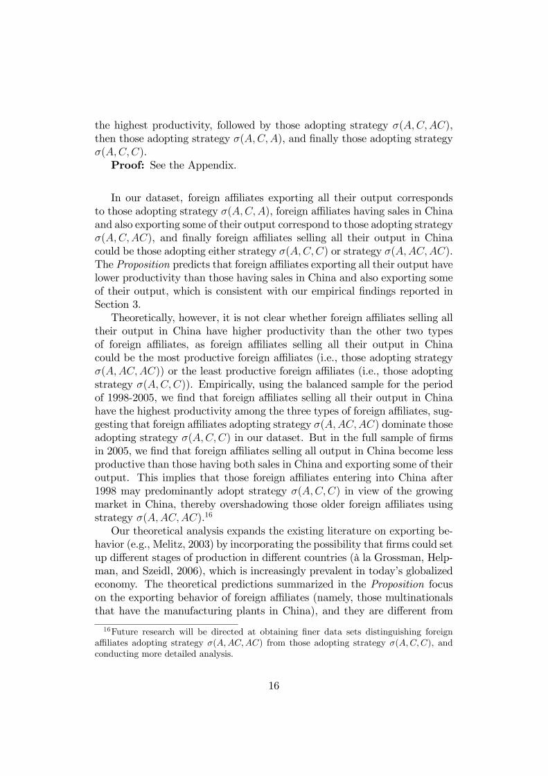
linear function of �, and it just di¤ers in the slope term (denoted by �) andthe intercept term (the negative of the �xed costs, denoted by F ) across thedi¤erent strategies (see the Figure for illustration).

14

The comparison of the �xed costs across the four strategies is straight-forward. Speci�cally, as strategy �(A;C;C) has design in the United Statesand manufacturing in China to serve the market in China, the �xed costs areequal to F�(A;C;C) � fAd + fCm + fs. Strategy �(A;C;A) involves design in theUnited States but manufacturing in China to serve the market in the UnitedStates, and so the �xed costs increase to F�(A;C;A) � fAd + fCm + fs+�fs dueto the extra selling costs involved when the market is served by manufac-turing plant located in a di¤erent country. Strategy �(A;C;AC) has designin the United States and manufacturing in China to serve both the marketin China and the market in the United States, and its �xed costs increasefurther to F�(A;C;AC) � fAd +fCm+2fs+�fs due to the additional selling costin China. Finally, strategy �(A;AC;AC) has design in the United States,and manufacturing plants in both the United States and China to serve therespective markets, and thus, compared with strategy �(A;C;AC), there isan increase in the manufacturing costs in the United States but a decrease inthe selling costs in the United States (i.e., F�(A;AC;AC) � fAd +fAm+fCm+2fs).It is expected that F�(A;AC;AC) is higher than F�(A;C;AC) as the additionalmanufacturing costs (fAm) are generally greater than the additional sellingcosts (�fs). So we have the following ranking of the �xed costs for thesefour strategies:

F�(A;C;C) < F�(A;C;A) < F�(A;C;AC) < F�(A;AC;AC): (4)

The slope term (�) is determined by the unit cost of production (thedenominator, C(:; :)) and the size of the markets (the nominator, I l, adjustedby relevant transport cost T ). For strategies �(A;C;C), �(A;C;A) and�(A;C;AC), they have the same unit cost of production, but di¤er in the sizeof the market. Assuming that the United States market is su¢ ciently largerthan the China market (i.e., I

A

T> IC), then the slope increases as one moves

from �(A;C;C) to �(A;C;A), and to �(A;C;AC). Strategy �(A;AC;AC)has the same size of the markets as strategy �(A;C;AC), but enjoys a lowerunit production cost than strategy �(A;C;AC) due to the tari¤-jumpingassumption. So we have the following ranking of the slope term for thesefour strategies:

��(A;C;C) < ��(A;C;A) < ��(A;C;AC) < ��(A;AC;AC): (5)

With inequalities (4) and (5), it follows that the optimal strategy for aforeign a¢ liate depends on its productivity:

Proposition: Given that neither the American market nor the Chinesemarket is negligible, foreign a¢ liates adopting strategy �(A;AC;AC) have

15

the highest productivity, followed by those adopting strategy �(A;C;AC),then those adopting strategy �(A;C;A), and �nally those adopting strategy�(A;C;C).Proof: See the Appendix.

In our dataset, foreign a¢ liates exporting all their output correspondsto those adopting strategy �(A;C;A), foreign a¢ liates having sales in Chinaand also exporting some of their output correspond to those adopting strategy�(A;C;AC), and �nally foreign a¢ liates selling all their output in Chinacould be those adopting either strategy �(A;C;C) or strategy �(A;AC;AC).The Proposition predicts that foreign a¢ liates exporting all their output havelower productivity than those having sales in China and also exporting someof their output, which is consistent with our empirical �ndings reported inSection 3.Theoretically, however, it is not clear whether foreign a¢ liates selling all

their output in China have higher productivity than the other two typesof foreign a¢ liates, as foreign a¢ liates selling all their output in Chinacould be the most productive foreign a¢ liates (i.e., those adopting strategy�(A;AC;AC)) or the least productive foreign a¢ liates (i.e., those adoptingstrategy �(A;C;C)). Empirically, using the balanced sample for the periodof 1998-2005, we �nd that foreign a¢ liates selling all their output in Chinahave the highest productivity among the three types of foreign a¢ liates, sug-gesting that foreign a¢ liates adopting strategy �(A;AC;AC) dominate thoseadopting strategy �(A;C;C) in our dataset. But in the full sample of �rmsin 2005, we �nd that foreign a¢ liates selling all output in China become lessproductive than those having both sales in China and exporting some of theiroutput. This implies that those foreign a¢ liates entering into China after1998 may predominantly adopt strategy �(A;C;C) in view of the growingmarket in China, thereby overshadowing those older foreign a¢ liates usingstrategy �(A;AC;AC).16

Our theoretical analysis expands the existing literature on exporting be-havior (e.g., Melitz, 2003) by incorporating the possibility that �rms could setup di¤erent stages of production in di¤erent countries (à la Grossman, Help-man, and Szeidl, 2006), which is increasingly prevalent in today�s globalizedeconomy. The theoretical predictions summarized in the Proposition focuson the exporting behavior of foreign a¢ liates (namely, those multinationalsthat have the manufacturing plants in China), and they are di¤erent from

16Future research will be directed at obtaining �ner data sets distinguishing foreigna¢ liates adopting strategy �(A;AC;AC) from those adopting strategy �(A;C;C), andconducting more detailed analysis.

16

the �ndings reported in the literature. It should be pointed out, however,that our theoretical framework can generate the same type of predictionson exporting behavior as in the existing literature if it is focused on domes-tic �rms (namely, �rms having both design and manufacturing in China).Among this type of �rms, it is the less productive ones that have domes-tic sales only while the more productive ones have both domestic sales andexport.

5 Conclusion

Firms have increasingly conducted di¤erent stages of production in di¤erentcountries (e.g., Hummels, Ishii, and Yi, 2001; Yi, 2003). In particular, theyhave set up operations in low-cost countries for labor-intensive production,and then used them as export platforms. As a result, a signi�cant percentageof export from those low-cost countries is made by foreign a¢ liates in thesecountries. Despite its importance, however, much of the existing literaturehas not formally examined the exporting behavior of foreign a¢ liates.In this paper, we �ll the void by empirically and theoretically investigating

the exporting behavior of foreign a¢ liates. Using annual surveys of manu-facturing �rms in China for the period of 1998 to 2005, we �nd that amongforeign a¢ liates in China exporters are less productive than non-exporters,in contrast to the unanimous �nding in the literature that exporters are moreproductive than non-exporters.To explain this puzzling �nding, we build up a standard trade model,

with �rm heterogeneity and location choices of vertically-related stages ofproduction (e.g., Melitz, 2003; Grossman, Helpman, and Szeidl, 2006). Wecan show that in equilibrium there are four strategies corresponding to thethree types of foreign a¢ liates observed in our dataset: foreign a¢ liates sell-ing all their output in China, foreign a¢ liates exporting all their output, andforeign a¢ liates having sales in China and exporting some of their output.The comparison among these four strategies in terms of their productivityo¤ers an explanation for our empirical �nding that among foreign a¢ liatesexporters are less productive than non-exporters.Our paper contributes to the growing literature of �rm heterogeneity and

trade by focusing on the exporting behavior of foreign a¢ liates, which areincreasingly prevalent in today�s globalized economy. To the best of ourknowledge, our study is the �rst one reporting that exporters are less pro-ductive than non-exporters. In addition, by incorporating into the standard�rm heterogeneity model (Melitz, 2003) the possibility that �rms could setup di¤erent stages of production in di¤erent countries (Grossman, Helpman,

17

and Szeidl, 2006), we are able to obtain much richer predictions on the rela-tion between �rm productivity and exporting behavior.

18

References

[1] Antràs, P. (2003). "Firms, Contracts, and Trade Structure." QuarterlyJournal of Economics 118: 1375-1418.

[2] Antràs, P. and E. Helpman (2004). "Global Sourcing." Journal of Po-litical Economy 112: 552-580.

[3] Baldwin, R.E., R. Forslid, P. Martin, G. Ottaviano, and F. Robert-Nicoud (2003). Economic Geography and Public Policy. Princeton Uni-versity Press.

[4] Baldwin, J. R. and W. Gu (2003). "Export-market participation andproductivity performance in Canadian manufacturing." Canadian Jour-nal of Economics 36(3): 634-657.

[5] Bernard, A. B., J. Eaton, J. B. Jensen, and S. Kortum (2003). "Plantsand Productivity in International Trade." American Economic Review93(4): 1268-1290.

[6] Bernard, A. B. and J. B. Jensen (1995). "Exporters, Jobs, and Wagesin the U.S. Manufacturing: 1976-1987." Brookings Papers on EconomicActivity: Microeconomics: 67-119.

[7] Bernard, A. B. and J. B. Jensen (1999). "Exceptional Exporter Perfor-mance: Cause, E¤ect, or Both?" Journal of International Economics47(1): 1-25.

[8] Bernard, A. B. and J. B. Jensen (2004). "Why Some Firms Export."Review of Economics and Statistics 86(2): 561-569.

[9] Bernard, A. B., J. B. Jensen, S. J. Redding, and P. K. Schott (2007)."Firms in International Trade." Journal of Economic Perspectives 21(3):105-130.

[10] Bernard, A. B., S. J. Redding, and P. K. Schott (2007). "Compara-tive Advantage and Heterogeneous Firms." Review of Economic Studies74(1): 31-66.

[11] Bernard, A. B. and J. Wagner (1997). "Exports and Success in GermanManufacturing." Weltwirtschaftliches Archiv 133: 134-157.

[12] Blalock, G. and P. J. Gertler (2004). "Learning from exporting revisitedin a less developed setting." Journal of Development Economics 75(2):397-416.

19

[13] Clerides, S. K., S. Lach, and J. R. Tybout (1998). "Is Learning by Ex-porting Important? Micro-Dynamic Evidence from Colombia, Mexico,and Morocco." Quarterly Journal of Economics 113(3): 903-947.

[14] De Loecker, J. (2007). "Do Exports Generate Higher Productivity? Evi-dence from Slovenia." Journal of International Economics 73(1): 69�98.

[15] Dixit, A.K. and J.E. Stiglitz. (1977). "Monopolistic Competition andOptimum Product Diversity." American Economic Review 67(3): 297-308.

[16] Eaton, J., S. Kortum, and F. Kramarz (2004). "Dissecting Trade: Firms,Industries, and Export Destinations." American Economic Review, Pa-pers and Proceedings 94(2): 150-154.

[17] Ekholm, K., R. Forslid, and J. Markusen. (2007). "Export-Platform For-eign Direct Investment.�Journal of the European Economic Association5: 776-795.

[18] Greene, William H. 2008. Econometric Analysis, Prentice Hall.

[19] Greenaway, D. and R. Kneller (2004). "Exporting and Productivity inthe United Kingdom." Oxford Review of Economic Policy 20(3): 358-371.

[20] Grossman, G. and E. Helpman (2005). "Outsourcing in a Global Econ-omy." Review of Economic Studies 72: 135-160.

[21] Grossman, G., E. Helpman, and A. Szeidl (2006). "Optimal IntegrationStrategies for the Multinational Firm." Journal of International Eco-nomics 70(1): 216-238.

[22] Hummels, D., J. Ishii, and K.M. Yi (2001). "The Nature and Growth ofVertical Specialization in World Trade." Journal of International Eco-nomics 54(1), 75-96.

[23] Kneller, R. and M. Pisu (2004). "Export-oriented FDI in the UK." Ox-ford Review of Economic Policy 20(3): 424-439.

[24] Levinsohn, J. and A. Petrin (2003). "Estimating Production FunctionsUsing Inputs to Control for Unobservables." Review of Economic Studies70(2): 317-342.

20

[25] Lu, J. and B. Xu (2009). "Foreign Direct Investment, Processing Trade,and China�s Export Sophistication." China Economic Review, forthcom-ing.

[26] Manova, K. and Z.W. Zhang (2008). "China�s Exporters and Importers:Firms, Products, and Trade Partners", working paper.

[27] Markusen, J. R. (2002). Multinational Firms and the Theory of Inter-national Trade. Cambridge, MA, MIT Press.

[28] Melitz, M. J. (2003). "The Impact of Trade on Intra-industry Real-locations and Aggregate Industry Productivity." Econometrica 71(6):1695-1725.

[29] Olley, G.S. and A. Pakes (1996). "The Dynamics of Productivity inthe Telecommunications Equipment Industry." Econometrica 64: 1263-1297.

[30] Rodrik, D. (2006). "What�s So Special about China�s Exports?" NBERWorking Paper No.11947.

[31] Van Biesebroeck, J. (2005). "Exporting Raises Productivity in Sub-Saharan African Manufacturing Firms." Journal of International Eco-nomics 67(2): 373-391.

[32] Van Biesebroeck, J. (2007). "Robustness of Productivity Estimates."Journal of Industrial Economics 55(3): 529-569.

[33] Van Biesebroeck, J. (2008). �The Sensitivity of Productivity Estimates:Revisiting Three Important Debates.� Journal of Business and Eco-nomic Statistics 26(3): 311-328.

[34] Wang, Z. and S.J. Wei. (2008). "What Accounts for the Rising Sophis-tication of China�s Exports?" NBER working paper w13771.

[35] Yeaple, S.R. (2003). "The Complex Integration Strategies of Multina-tionals and Cross Country Dependencies in the Structure of Foreign Di-rect Investment." Journal of International Economics 60(2): 293-314.

[36] Yi, K.M. (2003). "Can Vertical Specialization Explain the Growth ofWorld Trade?" Journal of Political Economy 111(1): 52-102.

21

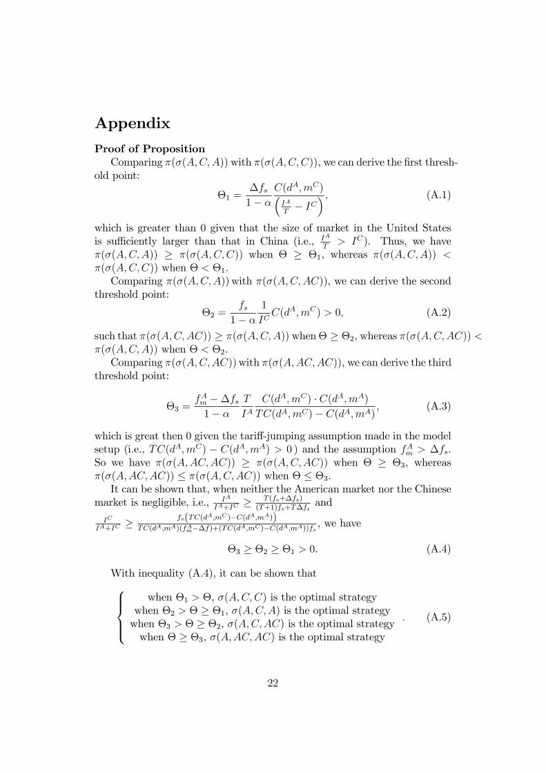
Appendix

Proof of PropositionComparing �(�(A;C;A)) with �(�(A;C;C)), we can derive the �rst thresh-

old point:

�1 =�fs1� �

C(dA;mC)�IA

T� IC

� ; (A.1)

which is greater than 0 given that the size of market in the United Statesis su¢ ciently larger than that in China (i.e., IA

T> IC). Thus, we have

�(�(A;C;A)) � �(�(A;C;C)) when � � �1, whereas �(�(A;C;A)) <�(�(A;C;C)) when � < �1.Comparing �(�(A;C;A))with �(�(A;C;AC)), we can derive the second

threshold point:

�2 =fs1� �

1

ICC(dA;mC) > 0; (A.2)

such that �(�(A;C;AC)) � �(�(A;C;A)) when� � �2, whereas �(�(A;C;AC)) <�(�(A;C;A)) when � < �2.Comparing �(�(A;C;AC))with �(�(A;AC;AC)), we can derive the third

threshold point:

�3 =fAm ��fs1� �

T

IAC(dA;mC) � C(dA;mA)

TC(dA;mC)� C(dA;mA); (A.3)

which is great then 0 given the tari¤-jumping assumption made in the modelsetup (i.e., TC(dA;mC) � C(dA;mA) > 0 ) and the assumption fAm > �fs.So we have �(�(A;AC;AC)) � �(�(A;C;AC)) when � � �3, whereas�(�(A;AC;AC)) � �(�(A;C;AC)) when � � �3.It can be shown that, when neither the American market nor the Chinese

market is negligible, i.e., IA

IA+IC� T (fs+�fs)

(T+1)fs+T�fsand

IC

IA+IC� fs(TC(dA;mC)�C(dA;mA))

TC(dA;mA)(fAm��f)+(TC(dA;mC)�C(dA;mA))fs, we have

�3 � �2 � �1 > 0. (A.4)

With inequality (A.4), it can be shown that8>><>>:when �1 > �, �(A;C;C) is the optimal strategy

when �2 > � � �1, �(A;C;A) is the optimal strategywhen �3 > � � �2, �(A;C;AC) is the optimal strategywhen � � �3, �(A;AC;AC) is the optimal strategy

: (A.5)

22

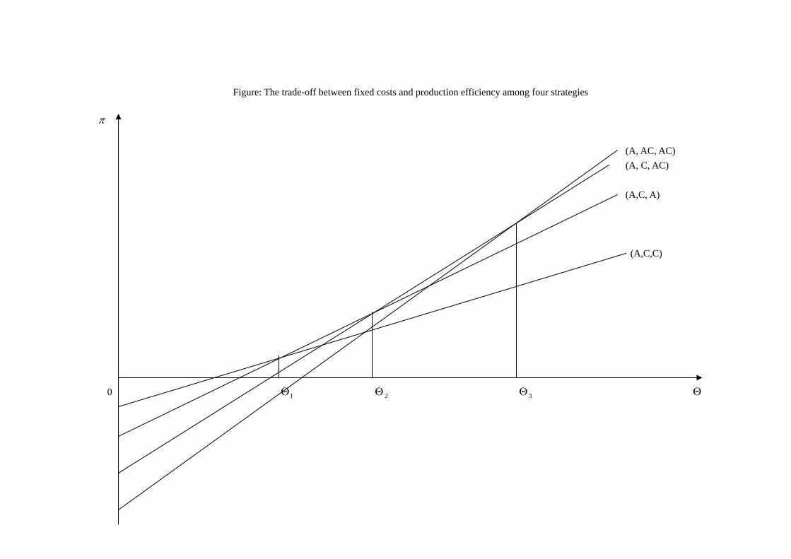
Figure: The trade-off between fixed costs and production efficiency among four strategies

(A, AC, AC) (A, C, AC)

(A,C, A)

(A,C,C)

0 1 2 3

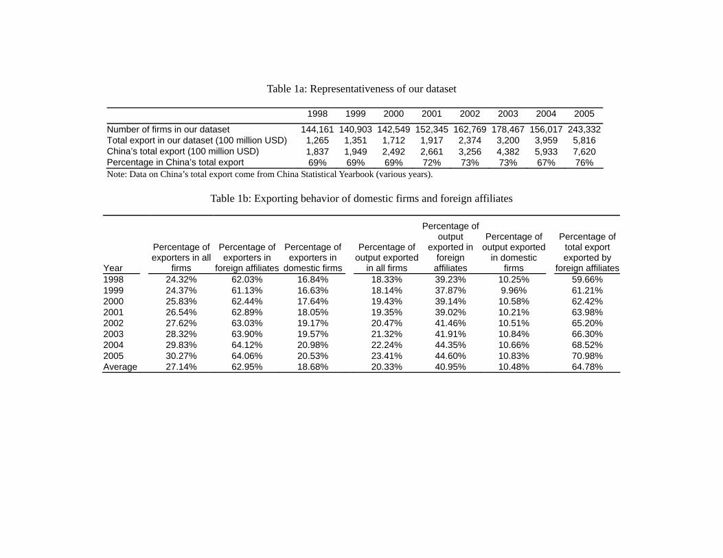
Table 1a: Representativeness of our dataset

1998 1999 2000 2001 2002 2003 2004 2005

Number of firms in our dataset 144,161 140,903 142,549 152,345 162,769 178,467 156,017 243,332Total export in our dataset (100 million USD) 1,265 1,351 1,712 1,917 2,374 3,200 3,959 5,816China’s total export (100 million USD) 1,837 1,949 2,492 2,661 3,256 4,382 5,933 7,620Percentage in China’s total export 69% 69% 69% 72% 73% 73% 67% 76% Note: Data on China’s total export come from China Statistical Yearbook (various years).

Table 1b: Exporting behavior of domestic firms and foreign affiliates

Year

Percentage of exporters in all

firms

Percentage of exporters in

foreign affiliates

Percentage of exporters in

domestic firms

Percentage of output exported

in all firms

Percentage of output

exported in foreign

affiliates

Percentage of output exported

in domestic firms

Percentage of total export exported by

foreign affiliates1998 24.32% 62.03% 16.84% 18.33% 39.23% 10.25% 59.66% 1999 24.37% 61.13% 16.63% 18.14% 37.87% 9.96% 61.21% 2000 25.83% 62.44% 17.64% 19.43% 39.14% 10.58% 62.42% 2001 26.54% 62.89% 18.05% 19.35% 39.02% 10.21% 63.98% 2002 27.62% 63.03% 19.17% 20.47% 41.46% 10.51% 65.20% 2003 28.32% 63.90% 19.57% 21.32% 41.91% 10.84% 66.30% 2004 29.83% 64.12% 20.98% 22.24% 44.35% 10.66% 68.52% 2005 30.27% 64.06% 20.53% 23.41% 44.60% 10.83% 70.98% Average 27.14% 62.95% 18.68% 20.33% 40.95% 10.48% 64.78%

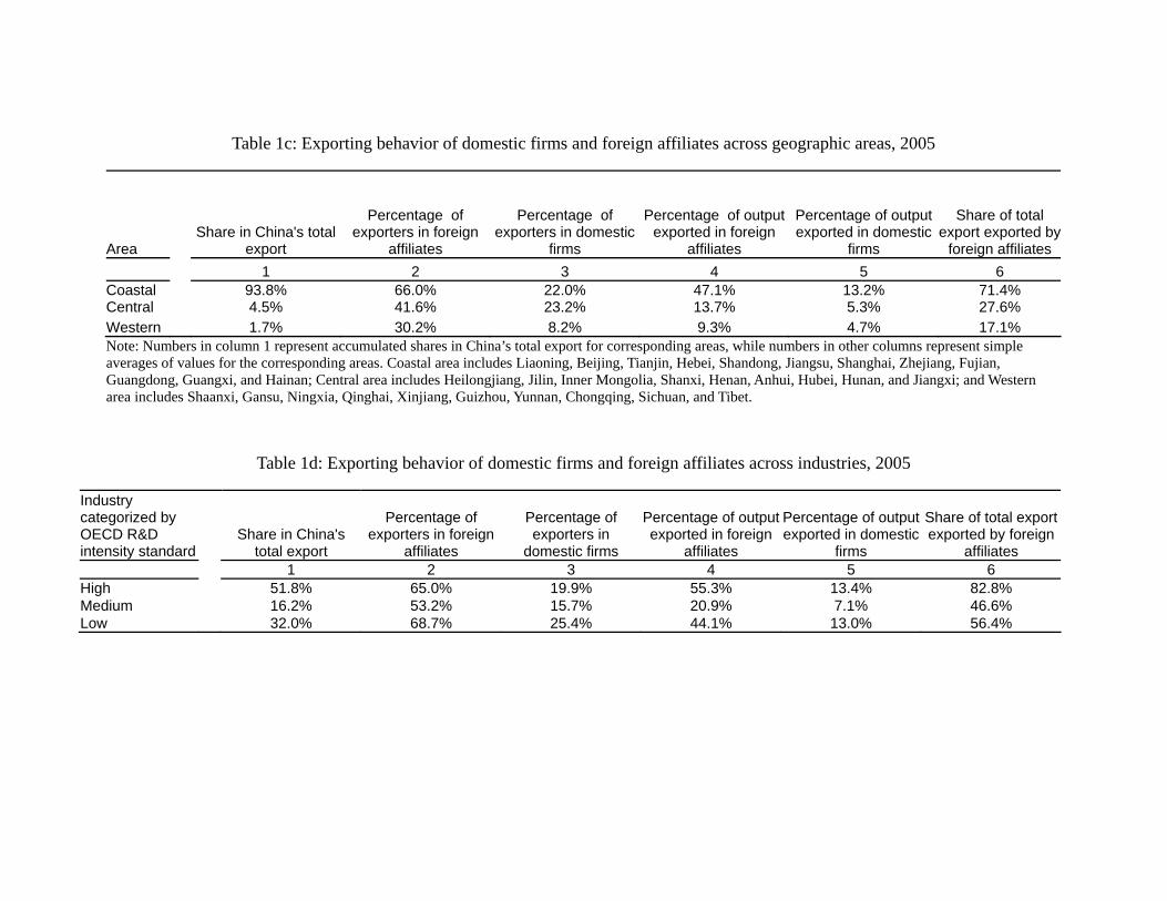
Table 1c: Exporting behavior of domestic firms and foreign affiliates across geographic areas, 2005

Area Share in China's total

export

Percentage of exporters in foreign

affiliates

Percentage of exporters in domestic

firms

Percentage of output exported in foreign

affiliates

Percentage of output exported in domestic

firms

Share of total export exported by

foreign affiliates 1 2 3 4 5 6 Coastal 93.8% 66.0% 22.0% 47.1% 13.2% 71.4% Central 4.5% 41.6% 23.2% 13.7% 5.3% 27.6% Western 1.7% 30.2% 8.2% 9.3% 4.7% 17.1% Note: Numbers in column 1 represent accumulated shares in China’s total export for corresponding areas, while numbers in other columns represent simple averages of values for the corresponding areas. Coastal area includes Liaoning, Beijing, Tianjin, Hebei, Shandong, Jiangsu, Shanghai, Zhejiang, Fujian, Guangdong, Guangxi, and Hainan; Central area includes Heilongjiang, Jilin, Inner Mongolia, Shanxi, Henan, Anhui, Hubei, Hunan, and Jiangxi; and Western area includes Shaanxi, Gansu, Ningxia, Qinghai, Xinjiang, Guizhou, Yunnan, Chongqing, Sichuan, and Tibet.

Table 1d: Exporting behavior of domestic firms and foreign affiliates across industries, 2005

Industry categorized by OECD R&D intensity standard

Share in China's total export

Percentage of exporters in foreign

affiliates

Percentage of exporters in

domestic firms

Percentage of output exported in foreign

affiliates

Percentage of output exported in domestic

firms

Share of total export exported by foreign

affiliates 1 2 3 4 5 6 High 51.8% 65.0% 19.9% 55.3% 13.4% 82.8% Medium 16.2% 53.2% 15.7% 20.9% 7.1% 46.6% Low 32.0% 68.7% 25.4% 44.1% 13.0% 56.4%

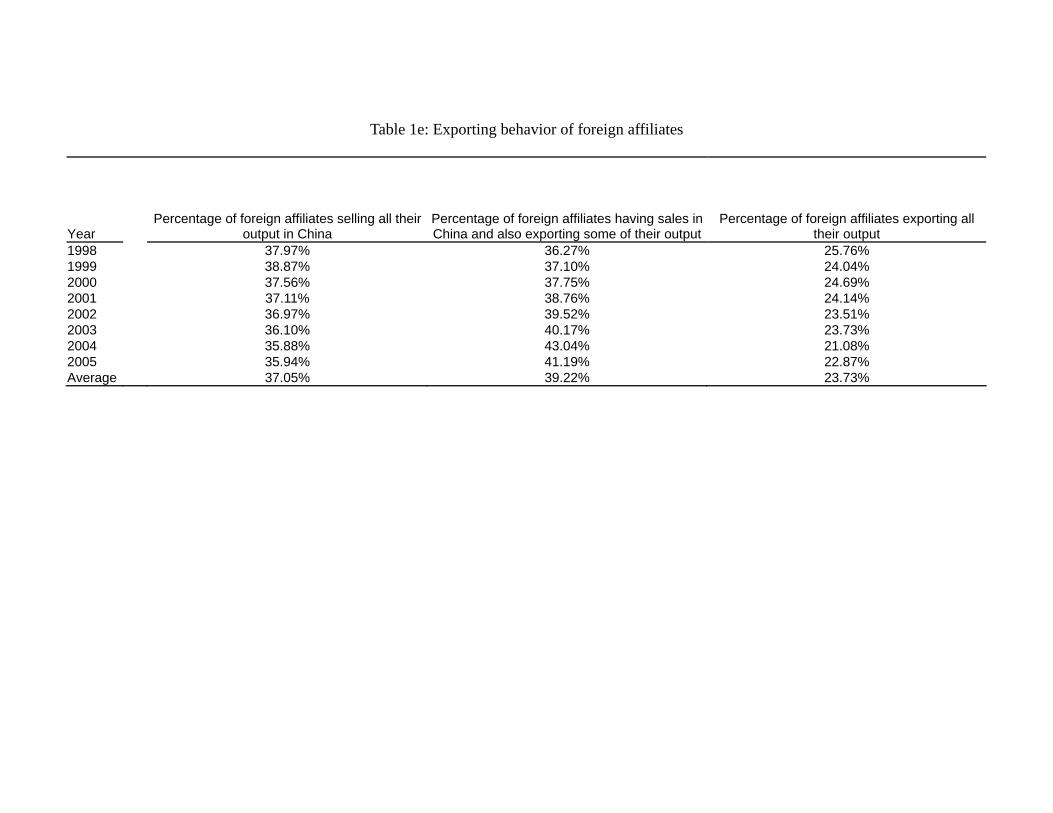
Table 1e: Exporting behavior of foreign affiliates

Year Percentage of foreign affiliates selling all their

output in China Percentage of foreign affiliates having sales in China and also exporting some of their output

Percentage of foreign affiliates exporting all their output

1998 37.97% 36.27% 25.76% 1999 38.87% 37.10% 24.04% 2000 37.56% 37.75% 24.69% 2001 37.11% 38.76% 24.14% 2002 36.97% 39.52% 23.51% 2003 36.10% 40.17% 23.73% 2004 35.88% 43.04% 21.08% 2005 35.94% 41.19% 22.87% Average 37.05% 39.22% 23.73%

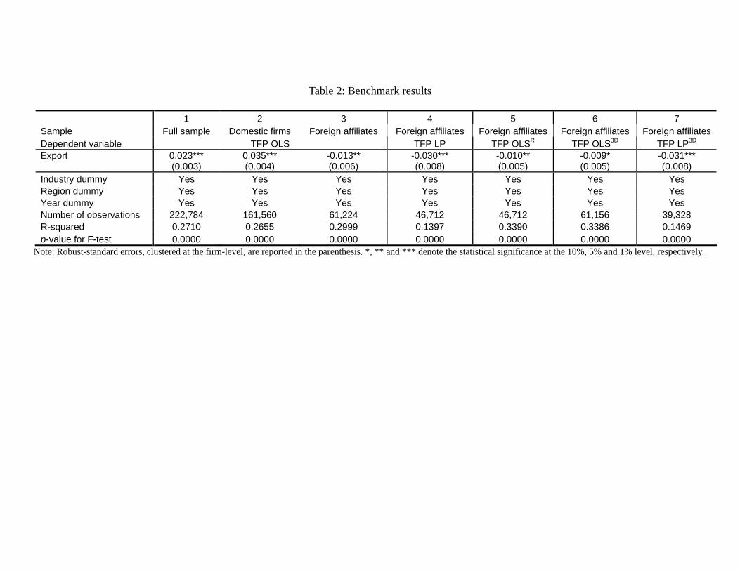
Table 2: Benchmark results

1 2 3 4 5 6 7 Sample Full sample Domestic firms Foreign affiliates Foreign affiliates Foreign affiliates Foreign affiliates Foreign affiliates Dependent variable TFP OLS TFP LP TFP OLSR TFP OLS3D TFP LP3D

Export 0.023*** (0.003)

0.035*** (0.004)

-0.013** (0.006)

-0.030*** (0.008)

-0.010** (0.005)

-0.009* (0.005)

-0.031*** (0.008)

Industry dummy Yes Yes Yes Yes Yes Yes Yes Region dummy Yes Yes Yes Yes Yes Yes Yes Year dummy Yes Yes Yes Yes Yes Yes Yes Number of observations 222,784 161,560 61,224 46,712 46,712 61,156 39,328 R-squared 0.2710 0.2655 0.2999 0.1397 0.3390 0.3386 0.1469 p-value for F-test 0.0000 0.0000 0.0000 0.0000 0.0000 0.0000 0.0000

Note: Robust-standard errors, clustered at the firm-level, are reported in the parenthesis. *, ** and *** denote the statistical significance at the 10%, 5% and 1% level, respectively.

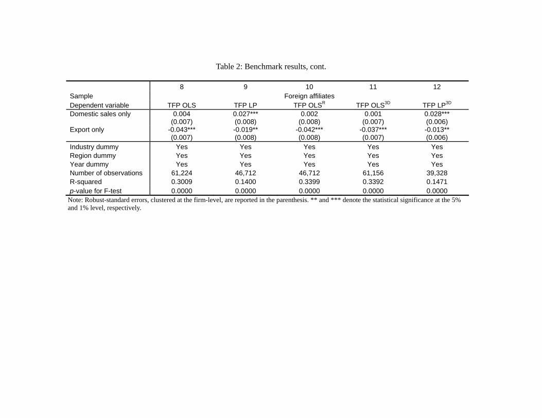
Table 2: Benchmark results, cont.

8 9 10 11 12 Sample Foreign affiliates Dependent variable TFP OLS TFP LP TFP OLSR TFP OLS3D TFP LP3D

Domestic sales only 0.004 (0.007)

0.027*** (0.008)

0.002 (0.008)

0.001 (0.007)

0.028*** (0.006)

Export only -0.043*** (0.007)

-0.019** (0.008)

-0.042*** (0.008)

-0.037*** (0.007)

-0.013** (0.006)

Industry dummy Yes Yes Yes Yes Yes Region dummy Yes Yes Yes Yes Yes Year dummy Yes Yes Yes Yes Yes Number of observations 61,224 46,712 46,712 61,156 39,328 R-squared 0.3009 0.1400 0.3399 0.3392 0.1471 p-value for F-test 0.0000 0.0000 0.0000 0.0000 0.0000

Note: Robust-standard errors, clustered at the firm-level, are reported in the parenthesis. ** and *** denote the statistical significance at the 5% and 1% level, respectively.

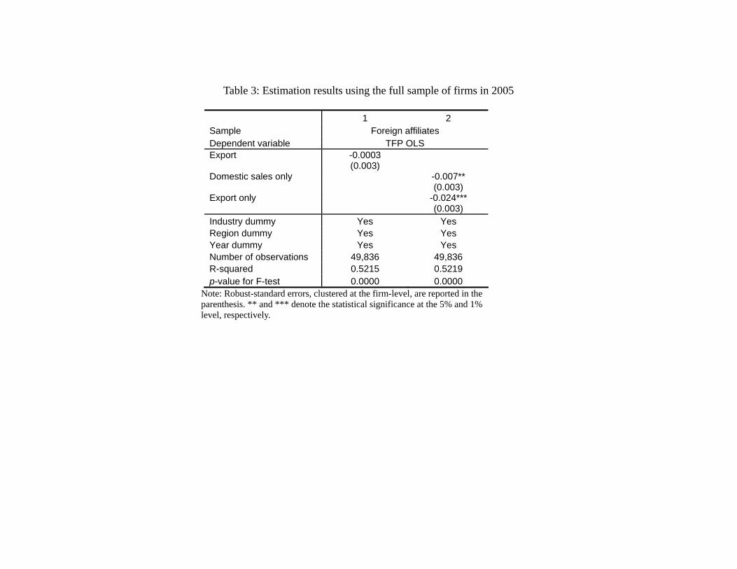
Table 3: Estimation results using the full sample of firms in 2005

1 2 Sample Foreign affiliates Dependent variable TFP OLS Export -0.0003

(0.003) Domestic sales only

-0.007** (0.003)

Export only

-0.024*** (0.003)

Industry dummy Yes Yes Region dummy Yes Yes Year dummy Yes Yes Number of observations 49,836 49,836 R-squared 0.5215 0.5219 p-value for F-test 0.0000 0.0000

Note: Robust-standard errors, clustered at the firm-level, are reported in the parenthesis. ** and *** denote the statistical significance at the 5% and 1% level, respectively.

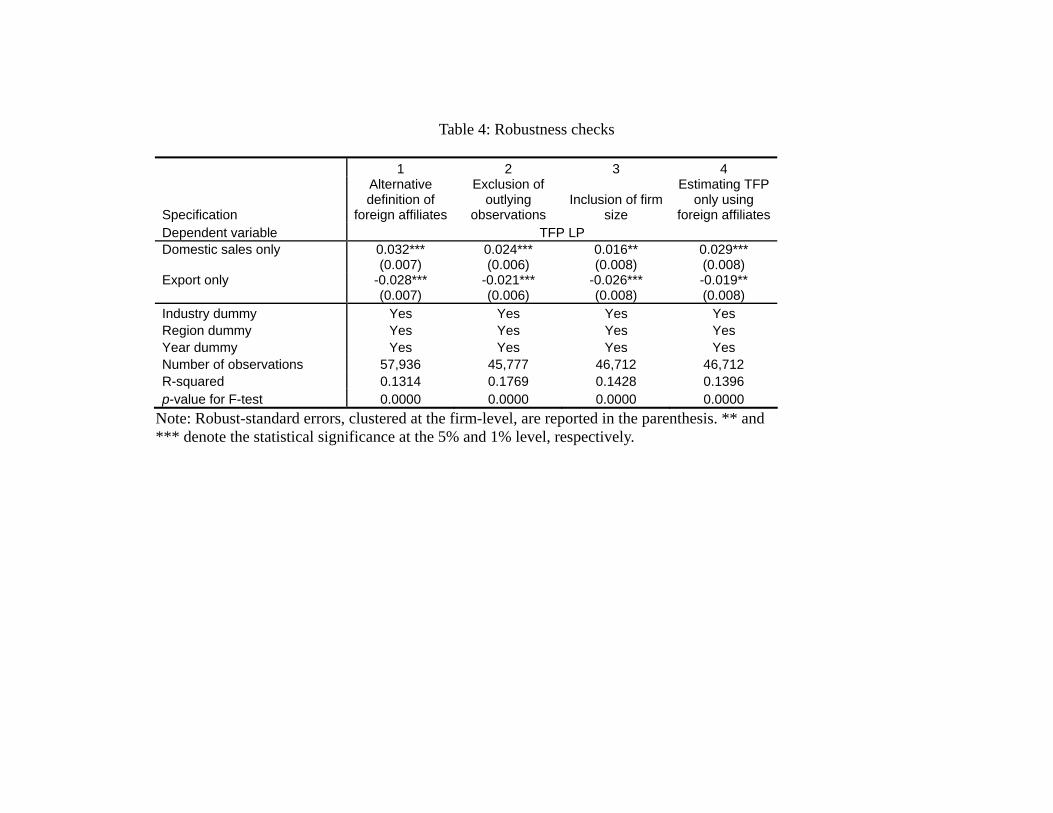
Table 4: Robustness checks

1 2 3 4

Specification

Alternative definition of

foreign affiliates

Exclusion of outlying

observations Inclusion of firm

size

Estimating TFP only using

foreign affiliatesDependent variable TFP LP Domestic sales only 0.032***

(0.007) 0.024*** (0.006)

0.016** (0.008)

0.029*** (0.008)

Export only -0.028*** (0.007)

-0.021*** (0.006)

-0.026*** (0.008)

-0.019** (0.008)

Industry dummy Yes Yes Yes Yes Region dummy Yes Yes Yes Yes Year dummy Yes Yes Yes Yes Number of observations 57,936 45,777 46,712 46,712 R-squared 0.1314 0.1769 0.1428 0.1396 p-value for F-test 0.0000 0.0000 0.0000 0.0000

Note: Robust-standard errors, clustered at the firm-level, are reported in the parenthesis. ** and *** denote the statistical significance at the 5% and 1% level, respectively.