1

Export Potential Assessments

A methodology to identify export opportunities for developing countries

Yvan Decreux and Julia Spies1

with contributions from Dzmitry Kniahin , Jie Sheng and Maria Del Mar Cantero

Draft version as of December 2016

Abstract In order to assist developing countries in identifying promising products for inclusion into export promotion activities, the International Trade Centre (ITC) has developed an export potential assessment methodology. It is based on a decomposition of a country’s potential exports of a product to a given target market into three factors: supply, demand and easiness to trade. Depending on the country’s particular needs, two approaches are available. (i) The Export Potential Indicator (EPI) serves countries that aim to support established export sectors in increasing their exports to existing and new markets. Inspired by a gravity-type framework, the EPI identifies products in which the exporting country has already proven to be internationally competitive and which have good prospects of export success in a given target market. (ii) The Product Diversification Indicator (PDI) serves countries that aim to diversify and develop new export sectors. Based on Hausmann and Hidalgo's notion of the product space, the PDI identifies products which the exporting country does not yet competitively export but which seem feasible given the country's current export basket and the export baskets of similar countries. Additional indicators that reflect policy objectives allow refining the selection of promising products. Results prove to be stable over time, turning them into a suitable information base for a country’s medium-term export strategies or development programmes.

1 The authors are highly indebted to the below listed colleagues for their valuable contributions. Lionel Fontagné has thoroughly reviewed the paper and provided comments that helped improving it considerably. Thanks go also to participants of seminars at ITC and WTO during which the methodology was presented and discussed.

2

Introduction

Purpose Trade and economic well-being rely on the availability and the sound governance of resources. Horizontal policies aiming at improving the efficiency of border procedures, harmonizing regulations on products and services, and increasing transparency of these rules are ways to create an environment that is conducive to an optimal use of resources. Nevertheless, governments do not limit themselves to horizontal policies but set up specialized agencies, seek developmental aid and negotiate trade rules that are by no means sector-neutral. Against this reality, Hausmann and Rodrik (2006) state that “interventions that increase the size and profitability of certain activities are legitimate if they contribute to the rest of society through taxes and higher productivity jobs” and conclude “we may be doomed to choose, but we should only choose when the maximum amount of information has been revealed.”

In order to bring transparency into the selection of products, sectors and markets for export promotion activities, the International Trade Centre (ITC) has developed an export potential assessment methodology. Based on detailed trade and market access information, it allows identifying – depending on the needs of the country – existing products with high export potential and/or diversification opportunities in a given target market:

The Export Potential Indicator (EPI) serves countries that aim to support established export sectors in increasing their exports to new or existing target markets. It identifies products in which the exporting country has already proven to be internationally competitive and which have good prospects of export success in specific target market(s) (intensive product margin).

The Product Diversification Indicator (PDI) serves countries that aim to diversify and develop new export sectors that face promising demand conditions in new or existing target markets. It identifies products which the exporting country does not yet export competitively but which seem feasible based on the country’s current export basket and the export baskets of similar countries (extensive product margin).

Conceptually, export potential assessments are based on the assumption that in a world without frictions trade flows can be described as a combination of supply performance, easiness to export and total demand. While a country’s capacity to supply existing products (EPI) is captured through projected market shares, its capacity to diversify into new products (PDI) relies on Hausmann and Hidalgo’s concept of the product space (Hausmann and Klinger, 2007, Hausmann et al., 2007 and Hidalgo et al., 2007) that establishes links between products through an assessment of how frequently they are found together in the export baskets of countries.

The first approach – the EPI – is based on a structural model that (i) identifies potential export values from supply capacities in the exporting country, demand conditions in the target market and bilateral linkages between the two. This corresponds to an empirical specification with exporter × product, importer × product and exporter × importer fixed effects but avoids computational constraints when working at a detailed product level.2 Any gap between what countries could export and what they actually do export is then argued to result from factors that trade advisors may address together with local companies, such as for example lacking information about the rules and regulations of the target market or difficulties in complying with them or in meeting the (quality) preferences of its consumers.

The second approach – the PDI – is based on the concept of the product space. The export potential assessment methodology improves the purely outcome-based measure of linkages to new products by accounting for natural endowments that are pivotal for the capacity of a country to produce certain

2 See Head and Mayer (2014).

3

products. It also responds to recent criticisms of the product space of being entirely supply-side driven (see e.g. Harrison and Rodriguez-Clare, 2011 or Lederman and Maloney, 2012) by combining it with demand and market access information. Since the descriptive nature of the product space does not allow for any meaningful estimate of potential trade values, we present rankings of diversification opportunities in a given country or regional market.

Very few attempts to give data-based guidance to developing countries on export opportunities have been made. One of them is the Decision Support Model (DSM) that starts by analysing the macroeconomic conditions of a large number of potential target markets and then, using a filtering approach, systematically screens possible product-market combinations (according to criteria such as import growth, size, market concentration and accessibility) until a shortlist of the most promising, ‘realistic’ opportunities remains (Cuyvers et al., 2012). The DSM differs from export potential assessments in that it relies on filters. Starting with all possible product-country combinations, it differentiates only at the end between products that fall within a country’s demonstrated export (supply) capacity and those that fall outside of it. In this way, new potential product-target market combinations are the residual of the filtering process and not derived from a dedicated approach to capture the extensive margin of trade. With the recent advances of the product space, a number of institutions (including UNCTAD and the World Bank) have started advising on diversification opportunities based on supply-side linkages between products. As mentioned above, these approaches disregard demand and market access factors that impact a country’s export decisions.

This paper starts with describing the methodology to measure the export and diversification potential of products in given target markets. It continues explaining in detail how data was processed and treated in order to achieve robust and reliable results for all countries in the world. For each product deemed “feasible”, indicators assessing its “desirability” from a social and developmental perspective are introduced. Finally, an exemplary output for one country, Iraq, is discussed along with checks of robustness based on all countries’ results.

Limitations Export potential assessments are a quantitative approach to identify promising export sectors and markets on a global scale, largely based on trade and market access data.

While the EPI is derived from a structural decomposition of trade into supply, demand and bilateral linkages and provides with an estimate of potential export values, the PDI is based on the descriptive, outcome-based concept of the product space. Export potential assessments therefore refrain from reporting any potential dollar value that could be associated with the identified diversification opportunities and provide only within-market ranks of products. In addition to the measurable components of export potential, there are other, often intangible, factors to consider when selecting sectors and products to target through trade development programmes. These include for example, the willingness and possibility to attract foreign direct investment, the possibilities of marketing and branding and the existence of synergic development plans or sector strategies. Export potential assessments also abstract from the costs related to export promotion activities. All of these factors may however influence the “feasibility” of exporting (more of) certain products. Trade advisors should therefore look at results with a critical eye and engage in further investigations notably with regards to the suggested options for diversification.

A few measurable indicators shed additional light upon the “desirability” of the identified products (e.g. does the product allow stabilizing export revenues? Does it support the participation of women?), but most developmental, environmental or social aspects cannot be captured with quantitative trade data. Often, they depend more on production practices than on the choice of products.

4

In light of these limitations, export potential assessments should be seen as a starting point in an export promotion decision-making process that needs to be followed up with further desk research and consultations with public and private sector stakeholders in the country.

Related literature Export potential assessments are linked to two different strands of trade literature. The EPI is based on the idea that trade between two countries is positively associated with the level of product supply and demand and negatively associated with trade impediments in the form of customs duties or geographic distance and naturally relates to gravity models. Early attempts to use the gravity model for predicting bilateral trade (especially in the context of East-West integration, see e.g. Wang and Winters, 1991; Baldwin, 1994 or Gros and Gonciarz, 1996) have been subject to fundamental critique. Egger (2002) argues that large deviations of actual from predicted trade rather indicate a misspecification of the model than an untapped opportunity and advocates out-of-sample estimations where the model is fitted on a reference group of countries. A few authors have used (out-of-sample) gravity models to determine sector trade potentials of certain countries. While some studies (e.g. Melchior et al., 2009 or Shepotylo, 2009) apply coefficients obtained from country characteristics to infer the potential trade of sectors, others (e.g. Fontagné et al., 2002; Helmers and Pasteels, 2006) suggest that without disaggregated information on the key determinants of sector level trade, results will be inaccurate. Product level production and consumption data however is not available and inferring these from exports and imports would introduce an endogeneity problem that eventually leads to biased coefficients.

More recently, theory-consistent in-sample estimation methods have gained prominence in the gravity literature (for a summary, see Head and Mayer, 2014). Cross-country and cross-sector specifications however would require the estimation of an enormous amount of coefficients and become computationally burdensome. Specifications with country-product, product-market and country-market fixed effects furthermore bear the disadvantage that the source of the potential export value remains opaque making results difficult to communicate to policymakers and trade advisers that may have most interest in using them. Predicting export potential values on the basis of detailed product level data therefore requires a different, more practical approach such as the one used in export potential assessments.

The PDI makes use of the concept of the product space as developed by Hausmann and Klinger (2007), Hausmann et al. (2007) and Hidalgo et al. (2007). In the framework of the product space countries will find it easier to venture into new products if they are frequently exported together with products that the country already exports. The underlying assumption is that these products require a set of capabilities similar to those that the country already possesses. A number of studies have applied this concept to provide guidance to developing countries on products they may become able to export in the future (for a recent example, see Fortunato et al., 2015). These studies have invariably focused on supply capacities without asking whether the suggested products have any prospect for export success in potential target markets.

To the best of our knowledge, the DSM is the only other approach that combines supply, demand and market access conditions in order to provide advice on export opportunities at a detailed product level. The DSM relies on a filtering process that eliminates unrealistic markets or products on a step-by-step basis. Trade potential values are consequently inferred from the market value of competitors in remaining product × market combinations, and are not derived from a structural model that accounts directly for the capacity of the exporter to supply a given target market. In the DSM, diversification opportunities comprise all products outside the country’s demonstrated supply capacity while export potential assessment identify and rank these opportunities based upon their linkages to the country’s current export basket and their chances of export success in given target markets.

5

6

Methodology Export potential assessments consist of two indicators: the EPI indicates potential export values of existing export products in a given target market. The PDI indicates relative ranks of product diversification opportunities in a given target market. The two indicators differ in the way supply capacities are captured. Demand and market access conditions are the same.

Export Potential Indicator3 The methodology to estimate export potential is inspired by a gravity model specified at the product level. The starting point is the assumption that in a world without frictions, trade flows could be described by a combination of exporter × product, importer × product and exporter × importer factors,

𝑣𝑖𝑗𝑘 = 𝛼𝑖𝑘𝛽𝑖𝑗𝛾𝑗𝑘 (1)

where 𝑣𝑖𝑗𝑘 corresponds to exports from exporter 𝑖 of product 𝑘 to market 𝑗. The parameter 𝛼𝑖𝑘

describes exporter 𝑖’s performance in exporting product 𝑘, 𝛾𝑗𝑘 market reflects 𝑗’s demand for product

𝑘 and 𝛽𝑖𝑗 the easiness to export any good from 𝑖 to 𝑗.

Equation (1) could be estimated econometrically and the differences between fitted and actual values may be interpreted as unused potential. The approach is inconvenient in this context for several reasons: first, the size of a model specified at the detailed product and country level would be very large. Second, the quality of three-dimensional data (𝑣𝑖𝑗𝑘) is low as experience shows that countries

find it difficult to accurately identify their trade partners. Third, in the absence of detailed production and consumption statistics, fixed effects would be used to capture 𝑖𝑘, 𝑖𝑗 and 𝑗𝑘 specific characteristics. A model estimated with fixed effects however makes communication about the drivers of the resulting export potential values difficult – a key requirement for achieving impact.

Export potential assessments therefore take a different approach and infer potential export values at 𝑖𝑗𝑘 level from a multiplicative model based on two-dimensional data,

𝑣𝑖𝑗�̃� = 𝛼𝑖�̃�𝛽𝑖�̃�𝑣𝑗𝑘 =𝑣𝑖𝑘

𝑣𝑘

𝑣𝑖𝑗

∑ (𝑣𝑖𝑘𝑣𝑘

𝑣𝑗𝑘)𝑘

𝑣𝑗𝑘 (2)

where the first term corresponds to exporter 𝑖’s world market share in product 𝑘. The second term is a measure of bilateral trade relative to what trade would be if the exporter had the same share in world markets as it has in market 𝑗. The third term simply reflects total imports. Annex I formally shows that in a world without frictions potential export values correspond to actual export values under certain assumptions:

Perfect competition within each country (supply is perfectly elastic but does not feature economies of scale);

Preferences specifying how imports of a given product are allocated among supplying countries are the same in all markets and take the form of a CES function;

Bilateral trade costs are ad valorem and do not depend on products;4

The average import price changes from market to market in the same proportion for all products;

3 Exporter-product combinations are considered to have export potential if they reach a total export potential value to the world of at least US$ 200,000 or if they are at least partly covered by the 95% cumulative export potential of products ranked in descending order for that exporter. Products below that threshold are perceived as having insufficient current potential but may be indicated as a diversification opportunity. 4 A correction is introduced later to take into account product-specific trade cost variations in the form of (i) tariffs and (ii) sensitivity to distance.

7

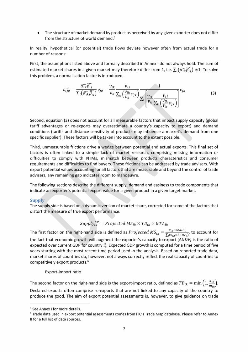
The structure of market demand by product as perceived by any given exporter does not differ from the structure of world demand.5

In reality, hypothetical (or potential) trade flows deviate however often from actual trade for a number of reasons:

First, the assumptions listed above and formally described in Annex I do not always hold. The sum of

estimated market shares in a given market may therefore differ from 1, i.e. ∑ (𝛼𝑖�̃�𝛽𝑖�̃�)𝑖 ≠1. To solve

this problem, a normalisation factor is introduced.

𝑣𝑖𝑗�̃� =

𝛼𝑖�̃�𝛽𝑖�̃�

∑ (𝛼𝑖�̃�𝛽𝑖�̃�)𝑖

𝑣𝑗𝑘 =𝑣𝑖𝑘

𝑣𝑘

𝑣𝑖𝑗

∑ (𝑣𝑖𝑘𝑣𝑘

𝑣𝑗𝑘)𝑘

1

∑ [𝑣𝑖𝑘𝑣𝑘

𝑣𝑖𝑗

∑ (𝑣𝑖𝑘𝑣𝑘

𝑣𝑗𝑘)𝑘

]𝑖

𝑣𝑗𝑘 (3)

Second, equation (3) does not account for all measurable factors that impact supply capacity (global tariff advantages or re-exports may overestimate a country’s capacity to export) and demand conditions (tariffs and distance sensitivity of products may influence a market’s demand from one specific supplier). These factors will be taken into account to the extent possible.

Third, unmeasurable frictions drive a wedge between potential and actual exports. This final set of factors is often linked to a simple lack of market research, comprising missing information or difficulties to comply with NTMs, mismatch between products characteristics and consumer requirements and difficulties to find buyers. These frictions can be addressed by trade advisers. With export potential values accounting for all factors that are measurable and beyond the control of trade advisers, any remaining gap indicates room to manoeuvre.

The following sections describe the different supply, demand and easiness to trade components that indicate an exporter’s potential export value for a given product in a given target market.

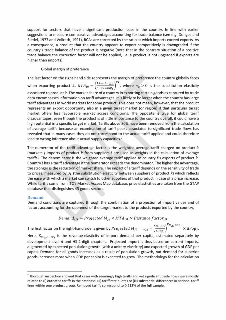
Supply The supply side is based on a dynamic version of market share, corrected for some of the factors that distort the measure of true export performance:

𝑆𝑢𝑝𝑝𝑙𝑦𝑖𝑘𝐸𝑃 = 𝑃𝑟𝑜𝑗𝑒𝑐𝑡𝑒𝑑 𝑀𝑆𝑖𝑘 × 𝑇𝐵𝑖𝑘 × 𝐺 𝑇𝐴𝑖𝑘

The first factor on the right-hand side is defined as 𝑃𝑟𝑜𝑗𝑒𝑐𝑡𝑒𝑑 𝑀𝑆𝑖𝑘 =𝑣𝑖𝑘×∆𝐺𝐷𝑃𝑖

∑ (𝑣𝑖𝑘×∆𝐺𝐷𝑃𝑖)𝑖, to account for

the fact that economic growth will augment the exporter’s capacity to export (∆𝐺𝐷𝑃𝑖 is the ratio of expected over current GDP for country 𝑖). Expected GDP growth is computed for a time period of five years starting with the most recent time period used in the analysis. Based on reported trade data, market shares of countries do, however, not always correctly reflect the real capacity of countries to competitively export products.6

Export-import ratio

The second factor on the right-hand side is the export-import ratio, defined as 𝑇𝐵𝑖𝑘 = min (1,𝑥𝑖𝑘

𝑚𝑖𝑘).

Declared exports often comprise re-exports that are not linked to any capacity of the country to produce the good. The aim of export potential assessments is, however, to give guidance on trade

5 See Annex I for more details. 6 Trade data used in export potential assessments comes from ITC’s Trade Map database. Please refer to Annex II for a full list of data sources.

8

support for sectors that have a significant production base in the country. In line with earlier suggestions to measure comparative advantages accounting for trade balance (see e.g. Donges and Riedel, 1977 and Vollrath, 1991), RCAs are corrected by the ratio at which imports exceed exports. As a consequence, a product that the country appears to export competitively is downgraded if the country’s trade balance of the product is negative (note that in the contrary situation of a positive trade balance the correction factor will not be applied, i.e. a product is not upgraded if exports are higher than imports).

Global margin of preference

The last factor on the right-hand side represents the margin of preference the country globally faces

when exporting product 𝑘, 𝐺 𝑇𝐴𝑖𝑘 = (1+av. tariff𝑖𝑘

1+av. tariff𝑘

)𝜎𝑘

, where 𝜎𝑘 > 0 is the substitution elasticity

associated to product 𝑘. The market share of a country in exporting certain goods as captured by trade data encompasses information on tariff advantages. It is likely to be larger when the country has large tariff advantages in world markets for some product. This does not mean, however, that the product represents an export opportunity also in a given target market (or region) if that particular target market offers less favourable market access conditions. The opposite is true for global tariff disadvantages: even though the product is of little importance to the country overall, it could have a high potential in a specific target market. Tariffs above 80% have been removed from the calculation of average tariffs because an examination of tariff peaks associated to significant trade flows has revealed that in many cases they do not correspond to the actual tariff applied and could therefore lead to wrong inference about actual supply capacities.7

The numerator of the tariff advantage factor is the weighted average tariff charged on product 𝑘 (markets 𝑗 imports of product 𝑘 from suppliers 𝑖 are used as weights in the calculation of average tariffs). The denominator is the weighted average tariff applied to country 𝑖’s exports of product 𝑘. Country 𝑖 has a tariff advantage if the numerator exceeds the denominator. The higher the advantage, the stronger is the reduction of market share. The impact of a tariff depends on the sensitivity of trade to prices, measured by 𝜎𝑘 (the substitution elasticity between suppliers of product k) which reflects the ease with which a market can switch to other suppliers of that product in case of a price increase. While tariffs come from ITC’s Market Access Map database, price elasticities are taken from the GTAP database that distinguishes 43 goods sectors.

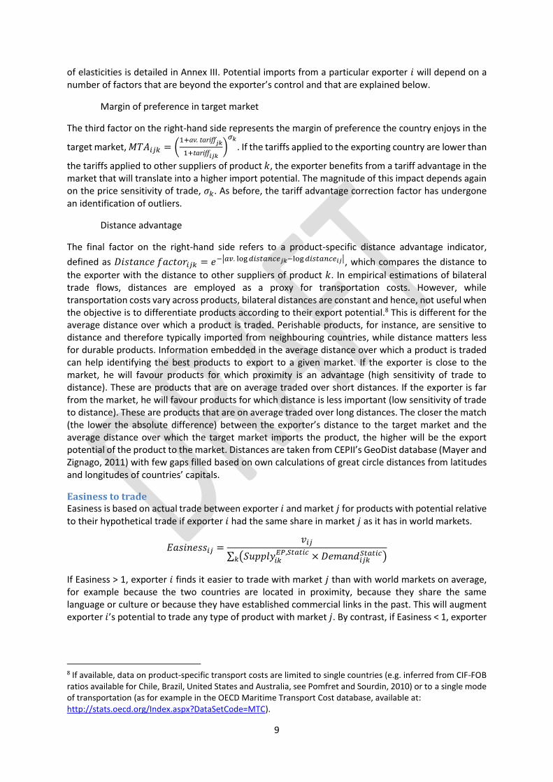
Demand Demand conditions are captured through the combination of a projection of import values and of factors accounting for the openness of the target market to the products exported by the country,

𝐷𝑒𝑚𝑎𝑛𝑑𝑖𝑗𝑘 = 𝑃𝑟𝑜𝑗𝑒𝑐𝑡𝑒𝑑 𝑀𝑗𝑘 × 𝑀 𝑇𝐴𝑖𝑗𝑘 × 𝐷𝑖𝑠𝑡𝑎𝑛𝑐𝑒 𝑓𝑎𝑐𝑡𝑜𝑟𝑖𝑗𝑘

The first factor on the right-hand side is given by 𝑃𝑟𝑜𝑗𝑒𝑐𝑡𝑒𝑑 𝑀𝑗𝑘 = 𝑣𝑗𝑘 × (∆GDP𝑗

∆Pop𝑗)

EM𝑑𝑐,GDP𝑗× ∆Pop𝑗.

Here, EM𝑑𝑐,GDP𝑗 is the revenue-elasticity of import demand per capita, estimated separately by

development level 𝑑 and HS 2-digit chapter 𝑐. Projected import is thus based on current imports, augmented by expected population growth (with a unitary elasticity) and expected growth of GDP per capita. Demand for all goods increases as a result of population growth, but demand for superior goods increases more when GDP per capita is expected to grow. The methodology for the calculation

7 Thorough inspection showed that cases with seemingly high tariffs and yet significant trade flows were mostly related to (i) outdated tariffs in the database, (ii) tariff rate quotas or (iii) substantial differences in national tariff lines within one product group. Removed tariffs correspond to 0.213% of the full sample.

9

of elasticities is detailed in Annex III. Potential imports from a particular exporter 𝑖 will depend on a number of factors that are beyond the exporter’s control and that are explained below.

Margin of preference in target market

The third factor on the right-hand side represents the margin of preference the country enjoys in the

target market, 𝑀𝑇𝐴𝑖𝑗𝑘 = (1+av. tariff𝑗𝑘

1+tariff𝑖𝑗𝑘

)𝜎𝑘

. If the tariffs applied to the exporting country are lower than

the tariffs applied to other suppliers of product 𝑘, the exporter benefits from a tariff advantage in the market that will translate into a higher import potential. The magnitude of this impact depends again on the price sensitivity of trade, 𝜎𝑘. As before, the tariff advantage correction factor has undergone an identification of outliers.

Distance advantage

The final factor on the right-hand side refers to a product-specific distance advantage indicator,

defined as 𝐷𝑖𝑠𝑡𝑎𝑛𝑐𝑒 𝑓𝑎𝑐𝑡𝑜𝑟𝑖𝑗𝑘 = 𝑒−|𝑎𝑣. log 𝑑𝑖𝑠𝑡𝑎𝑛𝑐𝑒𝑗𝑘−log 𝑑𝑖𝑠𝑡𝑎𝑛𝑐𝑒𝑖𝑗|, which compares the distance to

the exporter with the distance to other suppliers of product 𝑘. In empirical estimations of bilateral trade flows, distances are employed as a proxy for transportation costs. However, while transportation costs vary across products, bilateral distances are constant and hence, not useful when the objective is to differentiate products according to their export potential.8 This is different for the average distance over which a product is traded. Perishable products, for instance, are sensitive to distance and therefore typically imported from neighbouring countries, while distance matters less for durable products. Information embedded in the average distance over which a product is traded can help identifying the best products to export to a given market. If the exporter is close to the market, he will favour products for which proximity is an advantage (high sensitivity of trade to distance). These are products that are on average traded over short distances. If the exporter is far from the market, he will favour products for which distance is less important (low sensitivity of trade to distance). These are products that are on average traded over long distances. The closer the match (the lower the absolute difference) between the exporter’s distance to the target market and the average distance over which the target market imports the product, the higher will be the export potential of the product to the market. Distances are taken from CEPII’s GeoDist database (Mayer and Zignago, 2011) with few gaps filled based on own calculations of great circle distances from latitudes and longitudes of countries’ capitals.

Easiness to trade Easiness is based on actual trade between exporter 𝑖 and market 𝑗 for products with potential relative to their hypothetical trade if exporter 𝑖 had the same share in market 𝑗 as it has in world markets.

𝐸𝑎𝑠𝑖𝑛𝑒𝑠𝑠𝑖𝑗 =𝑣𝑖𝑗

∑ (𝑆𝑢𝑝𝑝𝑙𝑦𝑖𝑘𝐸𝑃,𝑆𝑡𝑎𝑡𝑖𝑐 × 𝐷𝑒𝑚𝑎𝑛𝑑𝑖𝑗𝑘

𝑆𝑡𝑎𝑡𝑖𝑐)𝑘

If Easiness > 1, exporter 𝑖 finds it easier to trade with market 𝑗 than with world markets on average, for example because the two countries are located in proximity, because they share the same language or culture or because they have established commercial links in the past. This will augment exporter 𝑖’s potential to trade any type of product with market 𝑗. By contrast, if Easiness < 1, exporter

8 If available, data on product-specific transport costs are limited to single countries (e.g. inferred from CIF-FOB ratios available for Chile, Brazil, United States and Australia, see Pomfret and Sourdin, 2010) or to a single mode of transportation (as for example in the OECD Maritime Transport Cost database, available at: http://stats.oecd.org/Index.aspx?DataSetCode=MTC).

10

𝑖 finds it relatively more difficult to trade with market 𝑗, lowering its potential to trade with that market irrespective of the product under analysis.

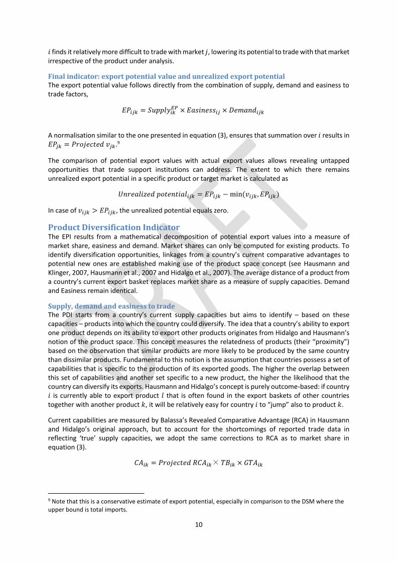
Final indicator: export potential value and unrealized export potential The export potential value follows directly from the combination of supply, demand and easiness to trade factors,

𝐸𝑃𝑖𝑗𝑘 = 𝑆𝑢𝑝𝑝𝑙𝑦𝑖𝑘𝐸𝑃 × 𝐸𝑎𝑠𝑖𝑛𝑒𝑠𝑠𝑖𝑗 × 𝐷𝑒𝑚𝑎𝑛𝑑𝑖𝑗𝑘

A normalisation similar to the one presented in equation (3), ensures that summation over 𝑖 results in 𝐸𝑃𝑗𝑘 = 𝑃𝑟𝑜𝑗𝑒𝑐𝑡𝑒𝑑 𝑣𝑗𝑘.9

The comparison of potential export values with actual export values allows revealing untapped opportunities that trade support institutions can address. The extent to which there remains unrealized export potential in a specific product or target market is calculated as

𝑈𝑛𝑟𝑒𝑎𝑙𝑖𝑧𝑒𝑑 𝑝𝑜𝑡𝑒𝑛𝑡𝑖𝑎𝑙𝑖𝑗𝑘 = 𝐸𝑃𝑖𝑗𝑘 − min (𝑣𝑖𝑗𝑘 , 𝐸𝑃𝑖𝑗𝑘)

In case of 𝑣𝑖𝑗𝑘 > 𝐸𝑃𝑖𝑗𝑘, the unrealized potential equals zero.

Product Diversification Indicator The EPI results from a mathematical decomposition of potential export values into a measure of market share, easiness and demand. Market shares can only be computed for existing products. To identify diversification opportunities, linkages from a country’s current comparative advantages to potential new ones are established making use of the product space concept (see Hausmann and Klinger, 2007, Hausmann et al., 2007 and Hidalgo et al., 2007). The average distance of a product from a country’s current export basket replaces market share as a measure of supply capacities. Demand and Easiness remain identical.

Supply, demand and easiness to trade The PDI starts from a country’s current supply capacities but aims to identify – based on these capacities – products into which the country could diversify. The idea that a country’s ability to export one product depends on its ability to export other products originates from Hidalgo and Hausmann’s notion of the product space. This concept measures the relatedness of products (their “proximity”) based on the observation that similar products are more likely to be produced by the same country than dissimilar products. Fundamental to this notion is the assumption that countries possess a set of capabilities that is specific to the production of its exported goods. The higher the overlap between this set of capabilities and another set specific to a new product, the higher the likelihood that the country can diversify its exports. Hausmann and Hidalgo’s concept is purely outcome-based: if country 𝑖 is currently able to export product 𝑙 that is often found in the export baskets of other countries together with another product 𝑘, it will be relatively easy for country 𝑖 to “jump” also to product 𝑘.

Current capabilities are measured by Balassa’s Revealed Comparative Advantage (RCA) in Hausmann and Hidalgo’s original approach, but to account for the shortcomings of reported trade data in reflecting ‘true’ supply capacities, we adopt the same corrections to RCA as to market share in equation (3).

𝐶𝐴𝑖𝑘 = 𝑃𝑟𝑜𝑗𝑒𝑐𝑡𝑒𝑑 𝑅𝐶𝐴𝑖𝑘× 𝑇𝐵𝑖𝑘 × 𝐺𝑇𝐴𝑖𝑘

9 Note that this is a conservative estimate of export potential, especially in comparison to the DSM where the upper bound is total imports.

11

where 𝑅𝐶𝐴𝑖𝑘 =𝑣𝑖𝑘

𝑣𝑘⁄

𝑣𝑘𝑣⁄

.

The link, 𝜑𝑘𝑙, from product k to product l is then defined based on the conditional probability 𝑃(. |. ) that a country has a comparative advantage in product 𝑘 if it already has one in product 𝑙:

𝜑𝑘𝑙 = 𝑃(𝐶𝐴𝑖𝑘′ |𝐶𝐴𝑖𝑙

′ ) ∀ 𝑖

where 𝐶𝐴𝑖𝑙′ = {

1 𝑖𝑓 𝐶𝐴𝑖𝑙 ≥ 1 0 𝑜𝑡ℎ𝑒𝑟𝑤𝑖𝑠𝑒

. 10 By using information on export bundles from all countries

worldwide, a measure of a country’s supply capacities can be calculated as the average proximity of a country to a new potential export product,

𝐷𝑒𝑛𝑠𝑖𝑡𝑦𝑖𝑘 =

∑ (𝐶𝐴𝑖𝑙′ 𝜑𝑘𝑙)𝑙

∑ 𝜑𝑘𝑙𝑙

A high density means that the country has developed comparative advantages in many products surrounding product 𝑘 and that product 𝑘 can be reached relatively easily. By contrast, a low value means that the product is far from the country’s current export structure and hence, an unlikely candidate for export diversification.

Even products with very high densities cannot necessarily be exported: first, the trade data-based measure of density cannot always correctly reflect endowments that are necessary to start producing and exporting new products. Boschma and Capone (2014) and Kniahin (2014) have assessed the predictive power of densities and shown that comparative advantages are positively associated with densities but that much of their variation is linked to other factors. For products strongly depending on natural resources the original product space approach is therefore modified to further refine suggested diversification opportunities:11

A GTAP dataset on land endowments has been exploited to detect the relevant moisture regimes and climatic zones enabling the exports of agricultural products. If a product is suggested for a country that does not possess any of the relevant land types, the product will not be considered as a feasible diversification opportunity (for details on this approach, see Annex IV).

Sea-related products that are currently not exported with comparative advantage and positive trade balance by any landlocked country are disregarded if suggested as diversification opportunities to landlocked countries.

Transformed products that are (almost) entirely based on excluded raw products from Chapter 71 (pearls, precious stones, metals, coins etc.) are not considered. Similarly, inorganic chemicals, precious metal compounds and isotopes (Chapter 28) are excluded because their

10 Note that the inventors of the product space suggest taking the minimum of both conditional probabilities 𝑃(𝐶𝐴′𝑖𝑙|𝐶𝐴′𝑖𝑘) and 𝑃(𝐶𝐴′𝑖𝑘|𝐶𝐴′𝑖𝑙) to avoid cases where a country is the only exporter of a particular good which would imply “that the conditional probability of exporting any other good given that one would be equal to one for all other goods exported by that country” (Hidalgo et al., 2007, p. 2 of the annex). In the context of this study both versions were computed and differences between them appear minimal. To save computational time and remain closer to the idea that linkages are based on a country’s current exports, unidirectional conditional probabilities are used. 11 Note that manufactured products are not filtered. Even though a country may currently not have the right resources to produce the good, it could invest (or receive foreign investment) into their future development thus bringing it closer to realizing the diversification potential.

12

production requires rare earths or other elements that may generally not be available in all countries.

Second, products that are feasible for the country may not be demanded by those markets with which the exporter finds it easy to trade. Or, even if they are in demand, the tariffs the exporter faces in this market may be unusually high. Harrison and Rodriguez-Clare (2011) and Lederman and Maloney (2012) argue that demand factors could be so favourable that being located in an isolated area of the product space (in particular if there is little competition) is preferable to being located in a dense area. This trade-off is not discussed in the original product space literature and disregarded in its applications. To identify diversification opportunities with good chances of export success, densities are combined with the same demand side and easiness to trade indicators that were used already in the EPI.

Final indicator: product diversification rank Densities differ from market shares in various ways and therefore have to be normalized before combining them with easiness and demand. First, the PDI supply indicator varies on a much smaller scale across products for a given country than corrected market shares and would therefore be given, if not adjusted, a small weight as compared to the demand side. The transformation 𝐷𝑒𝑛𝑠𝑖𝑡𝑦𝑖𝑘

′ =

𝐷𝑒𝑛𝑠𝑖𝑡𝑦𝑖𝑘

𝑙𝑜𝑔 𝑀𝑆𝑖𝑘1−𝑙𝑜𝑔 𝑀𝑆𝑖𝑘𝑁

𝑙𝑜𝑔 𝐷𝑒𝑛𝑠𝑖𝑡𝑦𝑖𝑘1−𝑙𝑜𝑔 𝐷𝑒𝑛𝑠𝑖𝑡𝑦𝑖𝑘𝑁 ensures that

𝐷𝑒𝑛𝑠𝑖𝑡𝑦𝑖𝑘1′

𝐷𝑒𝑛𝑠𝑖𝑡𝑦𝑖𝑘𝑁′ =

𝑀𝑆𝑖𝑘1

𝑀𝑆𝑖𝑘𝑁

, where 𝑁 is the rank of the last

product for which comparative advantage is computed and 𝑀𝑆𝑖𝑘 is the market share of country 𝑖 in the world market of product 𝑘. Note that accounting for the number of products that appear in the EPI of the country implies assuming that countries with a limited export basket also have limited capacity to diversify. Since these few products are spread over the full scale of comparative advantages, the density indicator (or, in other words, the supply side of the PDI) in countries with few current export products is given more weight than the density indicator in countries that have a big current export basket.

Second, while market shares are a relative concept, densities are an absolute measure meaning that many countries can have a high density around the same product. Therefore, the total diversification potential does not equal expected bilateral trade. Yet, a rough correspondence with total expected export capacity by country and total expected world demand by product is desirable. Densities are therefore rescaled in two steps:

𝐷𝑒𝑛𝑠𝑖𝑡𝑦𝑖𝑘′′ = 𝐷𝑒𝑛𝑠𝑖𝑡𝑦𝑖𝑘

′ ×∑ 𝐸𝑥𝑝 𝑣𝑖𝑗𝑘𝑗𝑘

∑ 𝑃𝐷𝐼𝑖𝑗𝑘𝑗𝑘 so that 𝑃𝐷𝑖

′ = 𝑃𝑟𝑜𝑗𝑒𝑐𝑡𝑒𝑑 𝑣𝑖

𝐷𝑒𝑛𝑠𝑖𝑡𝑦𝑖𝑘′′′ = 𝐷𝑒𝑛𝑠𝑖𝑡𝑦𝑖𝑘

′′ ×∑ 𝐸𝑥𝑝 𝑣𝑖𝑗𝑘𝑖𝑗

∑ 𝑃𝐷𝐼𝑖𝑗𝑘′

𝑖𝑗 so that 𝑃𝐷𝑘

′′ = 𝑃𝑟𝑜𝑗𝑒𝑐𝑡𝑒𝑑 𝑣𝑘

where 𝐸𝑥𝑝 𝑣 corresponds to trade augmented by expected GDP growth.

Assuming that the new supply indicator is given by normalised density, 𝑆𝑢𝑝𝑝𝑙𝑦𝑖𝑘𝑃𝐷 = 𝐷𝑒𝑛𝑠𝑖𝑡𝑦𝑖𝑘

′′′, and combining it with easiness to trade and demand gives:

𝑃𝐷𝑖𝑗𝑘 = 𝑆𝑢𝑝𝑝𝑙𝑦𝑖𝑘𝑃𝐷 × 𝐸𝑎𝑠𝑖𝑛𝑒𝑠𝑠𝑖𝑗 × 𝐷𝑒𝑚𝑎𝑛𝑑𝑖𝑗𝑘

A final normalisation is applied to 𝑆𝑢𝑝𝑝𝑙𝑦𝑖𝑘𝑃𝐷 × 𝐸𝑎𝑠𝑖𝑛𝑒𝑠𝑠𝑖𝑗 to ensure that market shares sum up to 1

in every market and 𝑃𝐷𝑗𝑘 = 𝑃𝑟𝑜𝑗𝑒𝑐𝑡𝑒𝑑 𝑣𝑗𝑘.12

12 Note that this normalization is sufficient to ensure 𝑃𝐷𝑘 = 𝑃𝑟𝑜𝑗𝑒𝑐𝑡𝑒𝑑 𝑣𝑘 but does not allow computing the factor 𝐷𝑒𝑛𝑠𝑖𝑡𝑦𝑖𝑘

′′′ that is visualized in the Export Potential Map tool (http://exportpotential.intracen.org).

13

As the resulting values are subject to much greater uncertainty than values originating from the export potential equation, only within market ranks of products are presented.

Aggregation and presentation of results Export and diversification potential values are calculated for every exporter × product × market combination. To aggregate to the level of sectors or regions, potential values can be simply summed up,

𝐸𝑃(𝑃𝐷)𝐼𝐽𝐾 = ∑ 𝐸𝑃(𝑃𝐷)𝑖𝑗𝑘

𝑖∈𝐼,𝑗∈𝐽,𝑘∈𝐾

In the EPI, the extent of unrealized potential can be aggregated as well:

𝑈𝑛𝑟𝑒𝑎𝑙𝑖𝑧𝑒𝑑 𝑝𝑜𝑡𝑒𝑛𝑡𝑖𝑎𝑙𝐼𝐽𝐾 = ∑ 𝐸𝑃𝑖𝑗𝑘

𝑖∈𝐼,𝑗∈𝐽,𝑘∈𝐾

− ∑ min (𝑣𝑖𝑗𝑘 , 𝐸𝑃𝑖𝑗𝑘)

𝑖∈𝐼,𝑗∈𝐽,𝑘∈𝐾

Taking the minimum ensures that overused potentials of some exporters, markets or products do not wipe out underused potentials elsewhere. Thus, only untapped potentials are aggregated to identify the extent of unrealized potential for a group of exporters, markets or products.

14

Data Export potential assessments can be implemented for any country and year for which trade data is available at a detailed product level. The following sections explain which data are used and how they are processed and cross-checked in order to obtain sound and reliable results.

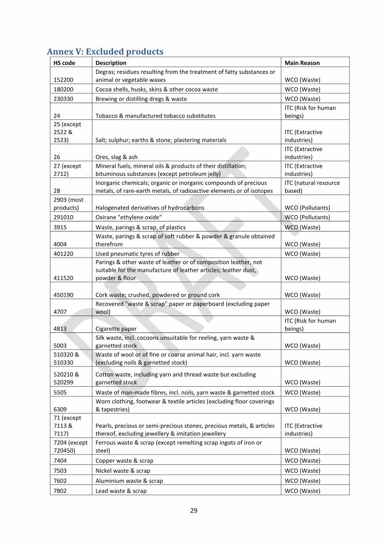
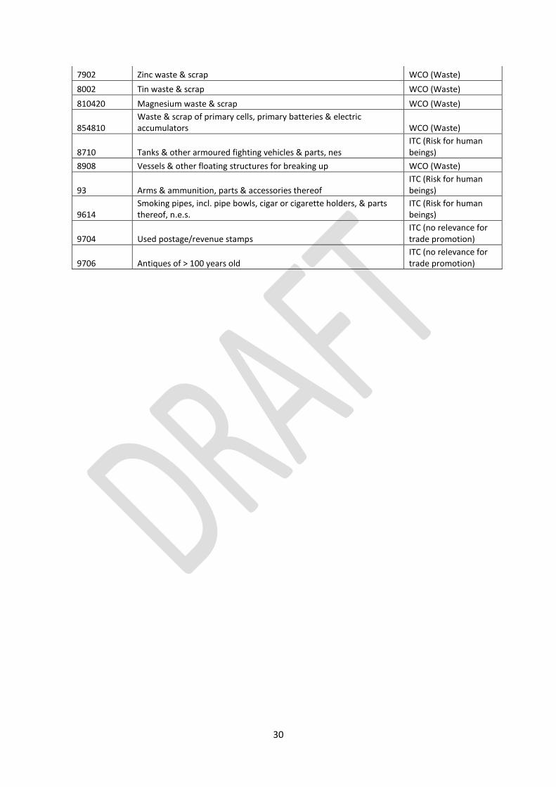
Coverage Trade data for 222 countries and territories comes from ITC’s Trade Map. The analyses start from the full list of products as defined at the 6-digit level of the Harmonized System (HS) classification; however, certain products not compatible with international conventions (e.g. products that have damaging effects on the environment)13, highly dependent on natural resources (extractive industries) or not in line with ITC’s work program (e.g. wastes, antiques, etc.) are excluded. Please refer to Annex V for a full list of excluded products. In light of revision changes of the HS, consistency across years and countries is achieved by introducing product groups that encompass all items that have ever fallen under the redefined HS code.14 There is one exception to this rule: product groups spread over different HS2 chapters are split into sub-groups so that every group fits within a single chapter. Manual checks have indicated that misallocations of trade in these cases are negligible. Export potential assessments therefore distinguish 4,034 HS 6-based product groups instead of the 5,205 HS 6 products that form the HS 2012 revision.15

Reliability of trade flows Four data reports are normally available for every country pair: country A’s declaration of exports to and imports from country B and country B’s declaration of exports to and imports from country A. Ideally, what A exports to B (as declared by country A) should match what B imports from A (as declared by country B) with only a small difference stemming from the fact that import values include insurance and freight costs (CIF) while export values are reported “free on board” (FOB). In reality, however, differences between direct reports and the so-called mirror reports are often substantial and it is not straightforward to identify the best source of data.

Export potential assessments aim to rank products according to their export or diversification potential. As these rankings could eventually determine to which projects public funds will be allocated, a major concern is the identification of “false positives”, thus projects that appear interesting from a data perspective but are in reality not very promising. Export potential assessments rely on a set of measures to ensure that misreported data does not affect the robustness of results: first, to even out bad data reports in single years, the sum of exports and imports over the past five years is used in the calculation of indicators. A product must be exported in the three most recent years, and imported in the five most recent years to remain in the analysis. Second, an iterative reliability check compares in every year a country’s reports of its exports and imports with those of its reliable trade partners. Reporters identified as unreliable are excluded from the next iteration and the process is repeated until the set of reliable reporters (by year and direction of trade flow) remains stable (for details, please see Annex VI). Third, for reliable data reporters, export potential assessments use a geometric average of both available data sources – direct and mirror reports – to mitigate the impact of misreported trade by one of the trade partners:16

13 The World Customs Organization (WCO) publishes correlation tables between the HS and several international conventions, available at: http://www.wcoomd.org/en/topics/nomenclature/instrument-and-tools/interconnection-table.aspx. 14 Note that HS 1992 (revision 0) is no longer in use. Product groups are therefore built on redefined codes between HS 1996 and HS 2012. 15 A correspondence table between HS 2012 6-digit codes and ITC product groups is available upon request. 16 There is one exception: bilateral trade data 𝑥𝑖𝑗𝑘 used to compute unused potential and total bilateral trade

rely on arithmetic averages of direct and mirror data because partners are often misidentified, so that using a geometric average would result in a significant reduction of trade flows. Furthermore, the concern of presenting

15

𝐸𝑠𝑡𝑖𝑚𝑎𝑡𝑒𝑑 𝑡𝑟𝑎𝑑𝑒 = √𝐷𝑖𝑟 × 𝑀𝑖𝑟

Compared to arithmetic averages, geometric averages downgrade products with big differences in reported trade, thus giving a more conservative estimate of the true trade value. In the extreme case of a country reporting exports of a given product while no partner country reports imports of that product, or of a country not confirming a flow reported by one or several of its partners, the estimated export value is zero. This is in line with the objective of export potential assessments to avoid listing products that are not confirmed by both sides.

With this method however, if a reporting country exports (imports) certain products exclusively to (from) partners that do not (reliably) report their trade, the geometric average for these products would be zero because all mirror flows would be zero. To avoid this, the estimated trade value relies on the geometric average of total direct flows to reliable reporting partners 𝑅𝐶 (and areas not elsewhere specified) and total mirror flows, and is augmented by total direct flows to non-reporting partners. Thus,

𝐸𝑠𝑡𝑖𝑚𝑎𝑡𝑒𝑑 𝑡𝑟𝑎𝑑𝑒𝑖(𝑗)𝑘 = √ ∑ 𝐷𝑖𝑟𝑖𝑗𝑘 × ∑ 𝑀𝑖𝑟𝑖𝑗𝑘

𝑗(𝑖)∈𝑅𝐶𝑗(𝑖)∈𝑅𝐶

+ ∑ 𝐷𝑖𝑟𝑖𝑗𝑘

𝑗(𝑖)∈𝑁𝑅𝐶

Missing data When data on tariffs, distances or GDP are missing, the following treatments are adopted:

Tariffs: in a few cases, countries report the tariffs they apply under the different tariff regimes in place but not on all products. The average tariff advantage or disadvantage the exporter faces in the country is then used for the products with missing tariff information.

Distances: gaps in the CEPII database are filled with great circle distances calculated from latitudes and longitudes of the country’s capitals. In extremely rare cases, bilateral distances are available but the distance indicator still cannot be calculated because markets import the product only from n.e.s. areas. These products are assigned the average distance correction factor for other products exported by the country to those markets.

Economic growth: if forecasts of the gross domestic product (GDP) are missing, the world GDP growth rate is used.

“false positives” does not apply for these values. As bilateral trade data are used to rescale potential shares and compute potential values, the overall magnitude of trade potentials is not affected by the choice of relying on geometric averages to compute potential shares.

16

Assessment of policy objectives The selected products may entail very different prospects for future economic development. Countries that want to meet certain policy objectives can narrow down their specific list of high potential export products through additional indicators that reflect whether the identified products are also “desirable” from a developmental perspective and associated policy considerations. A broad range of topics could be considered in this context. Four of the most common ones for which data are available are:

technology content

stability of export revenue

presence of SMEs and

participation of female employees

The objective of each additional indicator is to assess the product’s capacity to help the country improve along the measured dimension.

Technology content With input-output data not available for a wide range of countries, measures of technology intensity of products that rely on trade (and GDP) data only, have become popular. Hausmann, Hwang and Rodrik (2007) propose one the most commonly used indicators, the ‘PRODY,’ that calculates the weighted average per-capita income level associated with products, where the weights are Balassa’s RCAs. One of the inconveniences of the PRODY is that products of resource rich economies are associated with high GDP per capita levels even though their production may not be technology-intensive. Furthermore, using uncorrected RCAs gives a high weight to small countries that more often engage in re-exporting than large countries. The result is a product ranking that may overall be correlated with the technology intensity of production but is of limited use for giving specific advice as to which product exactly would help an exporter move up to more complex production stages in the global value chain.

We therefore modify the original PRODY and indicate products as technology-enhancing if the minimum GDP per capita level of the poorest country exporting them with comparative advantage and positive trade balance is at least as high or higher than exporter 𝑖’s per-capita GDP. Balassa RCA is corrected for overall tariff preferences: if a product is exported with a Balassa RCA only thanks to a preference on world markets, the country is not considered as having a comparative advantage in exporting that product.

𝑇𝐴𝑘 = 𝐷𝑖𝑘 min𝑖

𝐺𝐷𝑃𝑖

𝑃𝑜𝑝𝑖

where 𝐷𝑖𝑘 = {1 𝑖𝑓 𝑅𝐶𝐴𝑖𝑘 ≥ 1 𝑎𝑛𝑑 𝑇𝐵𝑖𝑘 > 0

0 𝑜𝑡ℎ𝑒𝑟𝑤𝑖𝑠𝑒.

Stability of export revenue Concentrating export promotion activities on products with strongly fluctuating prices can be a risky strategy for developing countries as it will confront them with unsecure and hardly predictable export revenues. Desirable products therefore feature rather stable prices. CEPII publishes annual trade unit values by HS 6 product and bilateral trading pair for the years 2003-2014. Each product group’s price volatility is measured as the standard deviation of its deflated average unit value in logarithms over the entire timeframe.17

17 Deflation is achieved by dividing the unit value by the mean unit value of all product groups in a given year.

17

A product is said to contribute to stability of export revenues if its prices have fluctuated less than the price of the country’s export basket on average over the considered timeframe.

Prospects for SMEs and female labour Even though the identified products are promising for the country overall, they may not favour the participation of all economic actors in the international value chain. Data from the World Bank Enterprise Surveys on

Firm size and

Permanent full-time female employees

are used to provide an indication of whether the sector under which the product group falls is predominantly made up of SMEs18 and employs many women.19 The information is currently available for 139 countries and 40 sectors distinguished in ISIC. To allocate the sector information from the enterprise surveys correctly to the ITC product groups, a correspondence between the two classifications has been established.

A product group is said to be favourable to the participation of SMEs and women if it belongs to a sector in which more SMEs or women are active than in the economy on average.

18 The World Bank Enterprise Surveys define SMEs as firms with 5 to 99 employees. 19 Note that data has been collected in different years. The indicator uses the latest available year per country.

18

Conclusion In response to the need of developing countries to learn about export opportunities, ITC has developed an export potential assessment methodology. Based on supply conditions at home and demand and market access conditions in target market(s), it brings transparency into and supports the selection of projects for export promotion activities. The methodology allows to either focus on products which the country already competitively exports (EPI) or on products which the country does not yet competitively export but which are likely candidates for diversification (PDI).

Conceptually, export potential assessments are based on a decomposition of potential export values into exporter × product, product × market and exporter × market factors. By this, they resemble a gravity equation specified at the product level while bypassing the latter’s computational problems. All analyses are based on data that has undergone a thorough treatment to ensure that results are not driven by misreported trade flows, measurement errors or wrong attribution. Elasticities establish the impact of each sub-indicator on potential export values. They are either taken from the literature or have been estimated exclusively for the purpose of the export potential assessment methodology. Robustness checks have shown that product rankings remain largely stable over time.

For each product listed in export potential assessments, additional indicators inform about the likelihood that it will help the country meet certain policy objectives, such as moving towards the exports of more technology-incorporating goods, stabilizing export revenues or increasing the presence of SMEs or of women in the economy.

In sum, backed up with sound scientific underpinnings, export potential assessments are a hands-on approach that provides guidance to governments and trade advisors in developing countries to

identify existing or new export opportunities, that are likely to generate high export revenues or offer untapped potentials, vis-à-vis a specific target market, a region or the entire world.

19

References Baldwin, R. (1994), Towards an Integrated Europe, Centre for Economic Policy Research, London.

Berthou, A., Emlinger, C. (2011), The Trade Unit Values Database, CEPII Working Paper 2011-10.

Boschma, R., Capone., G. (2014), Relatedness and Diversification in the EU-27 and ENP countries, Utrecht University Papers in Evolutionary Economic Geography 14.07.

Bussière, M., Callegari, G., Ghironi, F., Sestieri, G., Yamano, N. (2011), Estimating Trade Elasticities: Demand Composition and the Trade Collapse of 2008-09, American Economic Journal: Macroeconomics, American Economic Association, 5(3), 118-51.

Cuyvers, L., Steenkamp, E., Viviers, W. (2012), The methodology of the Decision Support Model (DSM), in: Cuyvers, L., Viviers, W. (eds.) Export Promotion: a Decision Support Model Approach. South Africa: Sun Media Metro.

Donges, J., Riedel, J. (1977), The expansion of manufactured exports in developing countries: An empirical assessment of supply and demand issues, Review of World Economics (Weltwirtschaftliches Archiv), 113(1), 58-87.

Egger, P. (2002), An Econometric View of the Estimation of Gravity Models and the Calculation of Trade Potentials, World Economy 25(2), 297-312.

Fontagné, L., Pajot, M., Pateels, J. (2002), Potentiels de commerce entre économies hétérogènes : un petit mode d’emploi des modèles de gravité, Economie internationale, 1(152-153), 115-139.

Fortunato, P., Razo, C., Vrolijk, K. (2015), Operationalizing the Product Space: A Road Map to Export Diversification, UNCTAD Discussion Papers No. 219.

Gros, D., Gonciarz, A. (1996), A note of the Trade Potential of Central and Eastern Europe, European Journal of Political Economy, 12(4): 709-721.

Harrison, A., Rodríguez-Clare, A. (2011), Trade, Foreign Investment, and Industrial Policy for Developing Countries, NBER Working Paper No. 15261.

Hausmann, R., Hwang, J., Rodrik, D. (2007), What you export matters, Journal of Economic Growth, 12(1): 1-25.

Hausmann, R., Rodrik, D. (2006), Doomed to choose: Industrial policy as predicament, Center for International Development Blue Sky Conference, September 9 2006, Cambridge, MA.

Hausmann, R., Klinger, B. (2007), Structural Transformation and Patterns of Comparative Advantage in the Product Space, Harvard Centre for International Development Working Paper No. 128.

Head, K., Mayer, T. (2014), Gravity Equations: Workhorse, Toolkit, and Cookbook, in: Gopinath, G., Helpman, E., Rogoff, K. (eds.) Handbook of International Economics vol. 4. Elsevier, 131-195.

Helmers. C., Pasteels, J. (2006), Assessing Bilateral Trade Potential at the Commodity Level: An Operational Approach, ITC Working Paper.

Hertel, T.H., Hummels, D., Ivanic, M., Keeney, R. (2004), How Confident Can We Be in CGE-Based Assessments of Free Trade Agreements?, GTAP Working Paper No. 26.

Hidalgo, C., Klinger, B., Barabasi, A.L., Hausmann, R. (2007), The product space conditions the development of nations, Science 317, 482-487.

20

Houthakker, H. S., Magee, P. (1969), Income and Price Elasticities in World Trade, The Review of Economics and Statistics, 51(2), 111-125.

Kniahin, D. (2014), Modeling International Trade Patterns with the Product Space Methodology, Master thesis.

Lederman, D., Maloney, W. (2012), Does What You Export Matter? In Search of Empirical Guidance for Industrial Policies, Washington, D.C.: The World Bank.

Mayer, T., Zignago, S. (2011), Notes on CEPII’s distances measures: the GeoDist Database, CEPII Working Paper 2011-25.

Melchior, A., Zheng, J., Johnsen, A. (2009), Trade barriers and export potential: Gravity estimates for Norway’s exports, Paper written for the Ministry of Trade and Industry, Norway.

Pomfret, R., Sourdin, P. (2010), Trade Facilitation and the Measurement of Trade Costs, Journal of International Commerce, Economics and Policy, 1(1), 145-163.

Shepotylo, O. (2009), Gravity with Zeros: Estimating Trade Potential of CIS countries, Kyiv School of Economics Discussion Paper No. 16.

Vollrath, T. (1991), A Theoretical Evaluation of Alternative Trade Intensity Measures of Revealed Comparative Advantage, Review of World Economics (Weltwirtschaftliches Archiv), 127(2).

Wang, Z., Winters, A. (1991), The Trading Potential of Eastern Europe, CEPR Discussion Paper No. 610.

21

Annex I: Theoretical underpinnings of the decomposition of potential export shares The export potential assessment methodology is based on the assumption that actual world trade differs from what it would be in a world without frictions (such as non-tariff trade obstacles). Its objective is to provide a means to estimate how trade flows would be distributed in this idealized world.

The paragraphs below show that under certain assumptions world trade values would take the following simple multiplicative form:

𝑣𝑖𝑗𝑘 = 𝛼𝑖𝑘𝛽𝑖𝑗𝛾𝑗𝑘

With:

𝑖 Exporting country

𝑗 Market

𝑘 Product (4,034 products based on the HS6 nomenclature)

𝑣𝑖𝑗𝑘 Trade value

The three factors can be interpreted as follows:

𝛼𝑖𝑘 Relative supply performance, in terms of cost and quality

𝛽𝑖𝑗 Relative easiness to export from country 𝑖 to market 𝑗

𝛾𝑗𝑘 Total demand

Potential trade is defined as what trade would be in this theoretical world. Potential trade can depart significantly from actual trade for a number of reasons: unseized opportunities, non-tariff measures, etc.

Model

Demand

Assumption 1: differentiation by supplier

Products exported by different exporters are perceived as different by consumers and companies purchasing them. For a given product, demand behaviour results from the optimization of a Constant Elasticity of Substitution (CES) function (Armington assumption).

CES functions are supposed to be the same in all markets. This assumption is necessary to derive a country’s capacity to export to a new market from its observed performance in other markets.

𝑣𝑖𝑗𝑘

𝑣𝑗𝑘= 𝛼𝑖𝑘 (

𝑝𝑗𝑘

𝑝𝑖𝑗𝑘)

𝜎𝑘−1

With ∑ 𝛼𝑖𝑘𝑖 = 1 (this assumption sets the price-volume split of the “composite good” but does not imply any additional restriction on demand behaviour).

Assumption 2: demand elasticity

While 𝑣𝑗𝑘 can be influenced by income growth in market 𝑗, it is assumed not to depend on prices (the

elasticity of aggregate import to aggregate price is supposed equal to 1).

22

Supply

Assumption 3: product homogeneity

Products exported by a given exporter to different markets are assumed to be the same.

Assumption 4: supply elasticity

Supply is assumed perfectly elastic: export prices do not depend on exported quantities.

Assumption 5: trade costs

𝑝𝑖𝑗𝑘 can be decomposed into a factor reflecting the production cost in country 𝑖 and a bilateral factor,

𝑝𝑖𝑗𝑘1−𝜎𝑘 = 휀𝑖𝑘𝜃𝑖𝑗

For simplicity, the volume of product 𝑘 exported by country 𝑖 is defined so that 휀𝑖𝑘 = 1. This does not imply any additional restriction. Any difference in cost or quality between two suppliers is reflected in the 𝛼𝑖𝑘 Armington parameter. Product-specific trade costs and barriers are introduced later.

Calculation The optimization of the CES function leads to:

𝑝𝑗𝑘1−𝜎𝑘 = ∑(𝛼𝑖𝑘𝑝𝑖𝑗𝑘

1−𝜎𝑘 )

𝑖

= ∑(𝛼𝑖𝑘𝜃𝑖𝑗)

𝑖

The price of composite good 𝑘 in market 𝑗 is higher if the trade costs of the most competitive suppliers (characterized by larger 𝛼𝑖𝑘) to that market are large (i.e. 𝜃𝑖𝑗 is small; for instance as a result of physical

or cultural distance between 𝑖 and 𝑗).

It follows:

𝑣𝑖𝑗𝑘 =

𝛼𝑖𝑘𝜃𝑖𝑗

∑ (𝛼𝑖𝑘𝜃𝑖𝑗)𝑖

𝑣𝑗𝑘 (A1)

Interpretation of the denominator: for a given demand 𝑣𝑗𝑘 and a given 𝛼𝑖𝑘 and 𝜃𝑖𝑗, the potential value

𝑣𝑖𝑗𝑘 is larger if the most competitive suppliers are “far” from market 𝑗.

Approximation 1:

𝑝𝑗𝑘1−𝜎𝑘 = ∑ (𝛼𝑖𝑘𝜃𝑖𝑗)𝑖 is assumed to depend only on the market: if a market is “far” from competitive

suppliers, it is assumed as “far” for all products.

∑(𝛼𝑖𝑘𝜃𝑖𝑗)

𝑖

= 𝜗𝑗

We define

𝛽𝑖𝑗 =𝜃𝑖𝑗

𝜗𝑗

Equation (A1) becomes

𝑣𝑖𝑗𝑘 = 𝛼𝑖𝑘𝛽𝑖𝑗𝑣𝑗𝑘

(A2)

23

Estimation

Strategy

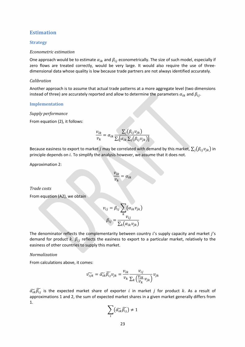
Econometric estimation

One approach would be to estimate 𝛼𝑖𝑘 and 𝛽𝑖𝑗 econometrically. The size of such model, especially if

zero flows are treated correctly, would be very large. It would also require the use of three-dimensional data whose quality is low because trade partners are not always identified accurately.

Calibration

Another approach is to assume that actual trade patterns at a more aggregate level (two dimensions instead of three) are accurately reported and allow to determine the parameters 𝛼𝑖𝑘 and 𝛽𝑖𝑗.

Implementation

Supply performance

From equation (2), it follows:

𝑣𝑖𝑘

𝑣𝑘= 𝛼𝑖𝑘

∑ (𝛽𝑖𝑗𝑣𝑗𝑘)𝑗

∑ [𝛼𝑖𝑘 ∑ (𝛽𝑖𝑗𝑣𝑗𝑘)𝑗 ]𝑖

Because easiness to export to market 𝑗 may be correlated with demand by this market, ∑ (𝛽𝑖𝑗𝑣𝑗𝑘)𝑗 in

principle depends on 𝑖. To simplify the analysis however, we assume that it does not.

Approximation 2:

𝑣𝑖𝑘

𝑣𝑘= 𝛼𝑖𝑘

Trade costs

From equation (A2), we obtain

𝑣𝑖𝑗 = 𝛽𝑖𝑗 ∑(𝛼𝑖𝑘𝑣𝑗𝑘)

𝑘

𝛽𝑖𝑗 =𝑣𝑖𝑗

∑ (𝛼𝑖𝑘𝑣𝑗𝑘)𝑘

The denominator reflects the complementarity between country 𝑖’s supply capacity and market 𝑗’s demand for product 𝑘. 𝛽𝑖𝑗 reflects the easiness to export to a particular market, relatively to the

easiness of other countries to supply this market.

Normalization

From calculations above, it comes:

𝑣𝑖𝑗�̃� = 𝛼𝑖�̃�𝛽𝑖�̃�𝑣𝑗𝑘 =𝑣𝑖𝑘

𝑣𝑘

𝑣𝑖𝑗

∑ (𝑣𝑖𝑘𝑣𝑘

𝑣𝑗𝑘)𝑘

𝑣𝑗𝑘

𝛼𝑖�̃�𝛽𝑖�̃� is the expected market share of exporter 𝑖 in market 𝑗 for product 𝑘. As a result of

approximations 1 and 2, the sum of expected market shares in a given market generally differs from 1.

∑(𝛼𝑖�̃�𝛽𝑖�̃�)

𝑖

≠ 1

24

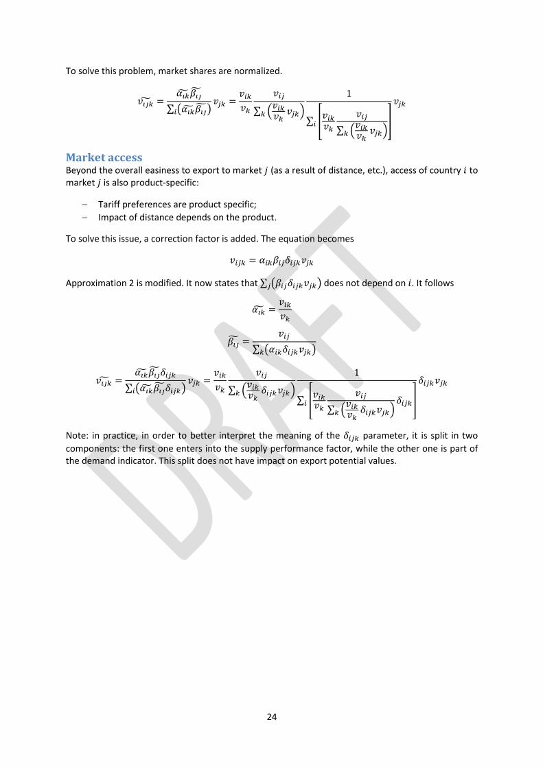
To solve this problem, market shares are normalized.

𝑣𝑖𝑗�̃� =𝛼𝑖�̃�𝛽𝑖�̃�

∑ (𝛼𝑖�̃�𝛽𝑖�̃�)𝑖

𝑣𝑗𝑘 =𝑣𝑖𝑘

𝑣𝑘

𝑣𝑖𝑗

∑ (𝑣𝑖𝑘𝑣𝑘

𝑣𝑗𝑘)𝑘

1

∑ [𝑣𝑖𝑘𝑣𝑘

𝑣𝑖𝑗

∑ (𝑣𝑖𝑘𝑣𝑘

𝑣𝑗𝑘)𝑘

]𝑖

𝑣𝑗𝑘

Market access Beyond the overall easiness to export to market 𝑗 (as a result of distance, etc.), access of country 𝑖 to market 𝑗 is also product-specific:

Tariff preferences are product specific;

Impact of distance depends on the product.

To solve this issue, a correction factor is added. The equation becomes

𝑣𝑖𝑗𝑘 = 𝛼𝑖𝑘𝛽𝑖𝑗𝛿𝑖𝑗𝑘𝑣𝑗𝑘

Approximation 2 is modified. It now states that ∑ (𝛽𝑖𝑗𝛿𝑖𝑗𝑘𝑣𝑗𝑘)𝑗 does not depend on 𝑖. It follows

𝛼𝑖�̃� =𝑣𝑖𝑘

𝑣𝑘

𝛽𝑖�̃� =𝑣𝑖𝑗

∑ (𝛼𝑖𝑘𝛿𝑖𝑗𝑘𝑣𝑗𝑘)𝑘

𝑣𝑖𝑗�̃� =𝛼𝑖�̃�𝛽𝑖�̃�𝛿𝑖𝑗𝑘

∑ (𝛼𝑖�̃�𝛽𝑖�̃�𝛿𝑖𝑗𝑘)𝑖

𝑣𝑗𝑘 =𝑣𝑖𝑘

𝑣𝑘

𝑣𝑖𝑗

∑ (𝑣𝑖𝑘𝑣𝑘

𝛿𝑖𝑗𝑘𝑣𝑗𝑘)𝑘

1

∑ [𝑣𝑖𝑘𝑣𝑘

𝑣𝑖𝑗

∑ (𝑣𝑖𝑘𝑣𝑘

𝛿𝑖𝑗𝑘𝑣𝑗𝑘)𝑘

𝛿𝑖𝑗𝑘]𝑖

𝛿𝑖𝑗𝑘𝑣𝑗𝑘

Note: in practice, in order to better interpret the meaning of the 𝛿𝑖𝑗𝑘 parameter, it is split in two

components: the first one enters into the supply performance factor, while the other one is part of the demand indicator. This split does not have impact on export potential values.

25

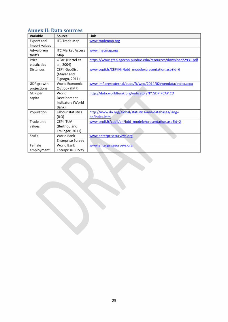
Annex II: Data sources Variable Source Link

Export and import values

ITC Trade Map www.trademap.org

Ad-valorem tariffs

ITC Market Access Map

www.macmap.org

Price elasticities

GTAP (Hertel et al., 2004)

https://www.gtap.agecon.purdue.edu/resources/download/2931.pdf

Distances CEPII GeoDist (Mayer and Zignago, 2011)

www.cepii.fr/CEPII/fr/bdd_modele/presentation.asp?id=6

GDP growth projections

World Economic Outlook (IMF)

www.imf.org/external/pubs/ft/weo/2014/02/weodata/index.aspx

GDP per capita

World Development Indicators (World Bank)

http://data.worldbank.org/indicator/NY.GDP.PCAP.CD

Population Labour statistics (ILO)

http://www.ilo.org/global/statistics-and-databases/lang--en/index.htm

Trade unit values

CEPII TUV (Berthou and Emlinger, 2011)

www.cepii.fr/cepii/en/bdd_modele/presentation.asp?id=2

SMEs World Bank Enterprise Survey

www.enterprisesurveys.org

Female employment

World Bank Enterprise Survey

www.enterprisesurveys.org

26

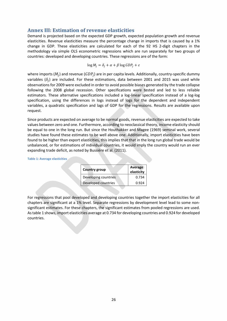
Annex III: Estimation of revenue elasticities Demand is projected based on the expected GDP growth, expected population growth and revenue elasticities. Revenue elasticities measure the percentage change in imports that is caused by a 1% change in GDP. These elasticities are calculated for each of the 92 HS 2-digit chapters in the methodology via simple OLS econometric regressions which are run separately for two groups of countries: developed and developing countries. These regressions are of the form:

log 𝑀𝑗 = 𝛿𝑗 + 𝛼 + 𝛽 log 𝐺𝐷𝑃𝑗 + 휀

where imports (𝑀𝑗) and revenue (𝐺𝐷𝑃𝑗) are in per capita levels. Additionally, country-specific dummy

variables (𝛿𝑗) are included. For these estimations, data between 2001 and 2015 was used while

observations for 2009 were excluded in order to avoid possible biases generated by the trade collapse following the 2008 global recession. Other specifications were tested and led to less reliable estimators. These alternative specifications included a log-linear specification instead of a log-log specification, using the differences in logs instead of logs for the dependent and independent variables, a quadratic specification and lags of GDP for the regressions. Results are available upon request.

Since products are expected on average to be normal goods, revenue elasticities are expected to take values between zero and one. Furthermore, according to neoclassical theory, income elasticity should be equal to one in the long run. But since the Houthakker and Magee (1969) seminal work, several studies have found these estimates to be well above one. Additionally, import elasticities have been found to be higher than export elasticities, this implies that that in the long run global trade would be unbalanced, or for estimations of individual countries, it would imply the country would run an ever expanding trade deficit, as noted by Bussière et al. (2011).

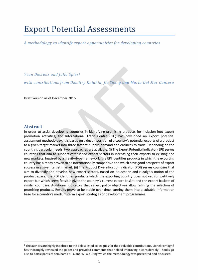
Table 1: Average elasticities

Country group Average elasticity

Developing countries 0.734

Developed countries 0.924

For regressions that pool developed and developing countries together the import elasticities for all chapters are significant at a 1% level. Separate regressions by development level lead to some non-significant estimates. For these chapters, the significant estimates from pooled regressions are used. As table 1 shows, import elasticities average at 0.734 for developing countries and 0.924 for developed countries.

27

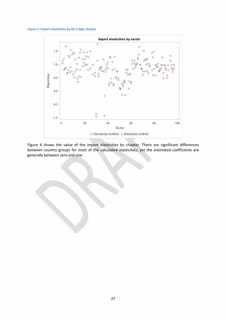
Figure 1: Import elasticities by HS 2-digit chapter

Figure 4 shows the value of the import elasticities by chapter. There are significant differences between country groups for most of the calculated elasticities, yet the estimated coefficients are generally between zero and one.

28

Annex IV: Land endowments The product space approach relies upon linkages between products inferred from trade data. But these linkages could result from a statistical coincidence without being truly related to production capacities (e.g. the mere fact that products 𝑙 and 𝑘 are jointly exported by many countries does not necessarily mean that any country currently exporting 𝑙 could also diversify into 𝑘). In order to refine the list of suggested products, information on actual endowments from a GTAP dataset that distinguishes 17 agro-ecological zones (AEZs) is used. AEZs are available for 114 individual countries and for all other countries at the level of their respective region. A country or region is considered as producing a product if it has exported it with comparative advantage and a strictly positive trade balance in the three most recent years of the analysis.

For each agricultural product (product groups 060110 to 140490, 1701, 1801, 4001, 4401 to 4403, 440710, 440722, 440725, 440726, 440791, 440792, 440910, 450110, 5201, 5202, 5301 to 5303), an iterative process identifies all land types suitable for its production. For each region we compute the rent associated with each land type and associate this information with the agricultural products exported by each region. By product we rank the land types in descending order of rent, and then enlarge the list of suitable land types one at a time until all current exporters are associated with this product.

With this method, between one and fourteen AEZs are considered as relevant for the production of a particular good. If the product space approach identifies strong links from the country’s current export basket to one of these products but the country does not possess any of the relevant AEZs, the product is removed from the list of feasible diversification opportunities for this country.

29

Annex V: Excluded products HS code Description Main Reason

152200 Degras; residues resulting from the treatment of fatty substances or animal or vegetable waxes WCO (Waste)

180200 Cocoa shells, husks, skins & other cocoa waste WCO (Waste)

230330 Brewing or distilling dregs & waste WCO (Waste)

24 Tobacco & manufactured tobacco substitutes ITC (Risk for human beings)

25 (except 2522 & 2523) Salt; sulphur; earths & stone; plastering materials

ITC (Extractive industries)

26 Ores, slag & ash ITC (Extractive industries)

27 (except 2712)

Mineral fuels, mineral oils & products of their distillation; bituminous substances (except petroleum jelly)

ITC (Extractive industries)

28 Inorganic chemicals; organic or inorganic compounds of precious metals, of rare-earth metals, of radioactive elements or of isotopes

ITC (natural resource based)

2903 (most products) Halogenated derivatives of hydrocarbons WCO (Pollutants)

291010 Oxirane "ethylene oxide" WCO (Pollutants)

3915 Waste, parings & scrap, of plastics WCO (Waste)

4004 Waste, parings & scrap of soft rubber & powder & granule obtained therefrom WCO (Waste)

401220 Used pneumatic tyres of rubber WCO (Waste)

411520

Parings & other waste of leather or of composition leather, not suitable for the manufacture of leather articles; leather dust, powder & flour WCO (Waste)

450190 Cork waste; crushed, powdered or ground cork WCO (Waste)

4707 Recovered "waste & scrap" paper or paperboard (excluding paper wool) WCO (Waste)

4813 Cigarette paper ITC (Risk for human beings)

5003 Silk waste, incl. cocoons unsuitable for reeling, yarn waste & garnetted stock WCO (Waste)

510320 & 510330

Waste of wool or of fine or coarse animal hair, incl. yarn waste (excluding noils & garnetted stock) WCO (Waste)

520210 & 520299

Cotton waste, including yarn and thread waste but excluding garnetted stock WCO (Waste)

5505 Waste of man-made fibres, incl. noils, yarn waste & garnetted stock WCO (Waste)

6309 Worn clothing, footwear & textile articles (excluding floor coverings & tapestries) WCO (Waste)

71 (except 7113 & 7117)

Pearls, precious or semi-precious stones, precious metals, & articles thereof, excluding jewellery & imitation jewellery

ITC (Extractive industries)

7204 (except 720450)

Ferrous waste & scrap (except remelting scrap ingots of iron or steel) WCO (Waste)

7404 Copper waste & scrap WCO (Waste)

7503 Nickel waste & scrap WCO (Waste)

7602 Aluminium waste & scrap WCO (Waste)

7802 Lead waste & scrap WCO (Waste)

30

7902 Zinc waste & scrap WCO (Waste)

8002 Tin waste & scrap WCO (Waste)

810420 Magnesium waste & scrap WCO (Waste)

854810 Waste & scrap of primary cells, primary batteries & electric accumulators WCO (Waste)

8710 Tanks & other armoured fighting vehicles & parts, nes ITC (Risk for human beings)

8908 Vessels & other floating structures for breaking up WCO (Waste)

93 Arms & ammunition, parts & accessories thereof ITC (Risk for human beings)

9614 Smoking pipes, incl. pipe bowls, cigar or cigarette holders, & parts thereof, n.e.s.

ITC (Risk for human beings)

9704 Used postage/revenue stamps ITC (no relevance for trade promotion)

9706 Antiques of > 100 years old ITC (no relevance for trade promotion)

31

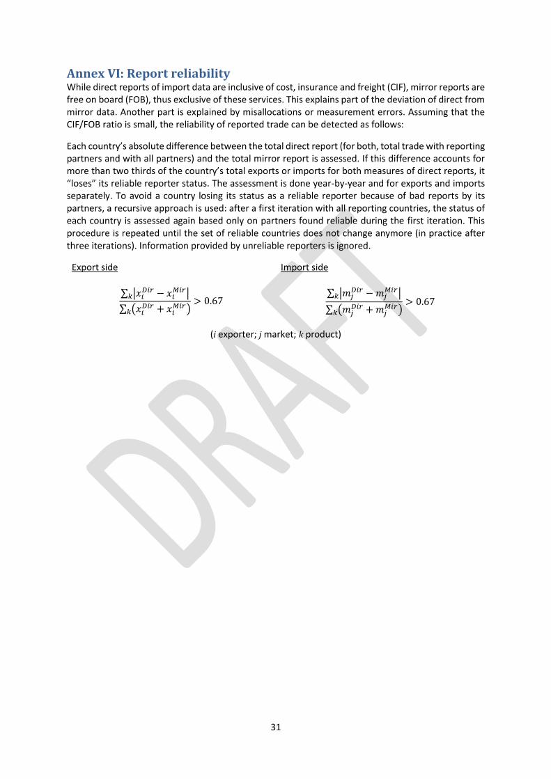
Annex VI: Report reliability While direct reports of import data are inclusive of cost, insurance and freight (CIF), mirror reports are free on board (FOB), thus exclusive of these services. This explains part of the deviation of direct from mirror data. Another part is explained by misallocations or measurement errors. Assuming that the CIF/FOB ratio is small, the reliability of reported trade can be detected as follows:

Each country’s absolute difference between the total direct report (for both, total trade with reporting partners and with all partners) and the total mirror report is assessed. If this difference accounts for more than two thirds of the country’s total exports or imports for both measures of direct reports, it “loses” its reliable reporter status. The assessment is done year-by-year and for exports and imports separately. To avoid a country losing its status as a reliable reporter because of bad reports by its partners, a recursive approach is used: after a first iteration with all reporting countries, the status of each country is assessed again based only on partners found reliable during the first iteration. This procedure is repeated until the set of reliable countries does not change anymore (in practice after three iterations). Information provided by unreliable reporters is ignored.

Export side

Import side

∑ |𝑥𝑖𝐷𝑖𝑟 − 𝑥𝑖

𝑀𝑖𝑟|𝑘

∑ (𝑥𝑖𝐷𝑖𝑟 + 𝑥𝑖

𝑀𝑖𝑟)𝑘

> 0.67

∑ |𝑚𝑗𝐷𝑖𝑟 − 𝑚𝑗

𝑀𝑖𝑟|𝑘

∑ (𝑚𝑗𝐷𝑖𝑟 + 𝑚𝑗

𝑀𝑖𝑟)𝑘

> 0.67

(i exporter; j market; k product)