Export Diversification Effects of the WTO Trade

The ‘center of excellence’ FIW (http://www.fiw.ac.at/), is a project of WIFO, wiiw, WSR and Vienna University of Economics and Business, University of Vienna, Johannes Kepler University Linz on behalf of the BMWFW

FIW – Working Paper

Export Diversification Effects of the WTO Trade Facilitation Agreement

Cosimo Beverelli1

Simon Neumueller2

Robert Teh3

We estimate the effects of trade facilitation on export diversification, as measured by two extensive margins: the number of products exported by destination and the number of export destinations served by product. To address the issue of causality, we employ an identification strategy whereby only exports of new products, or exports to new destinations, are taken into account when computing the respective margins of trade. We find a positive impact of trade facilitation on the extensive margins of trade. The results are robust to alternative definitions of extensive margins, different sets of controls and various estimation methods. Simulation results suggest substantial extensive margin gains from trade facilitation reform in Sub-Saharan Africa and Latin America and the Caribbean. JEL : F13, F14, F17 Keywords: Trade facilitation, Export diversification, International trade

agreements, WTO

1 Economic Research Division, World Trade Organization, 1211 Geneva, Switzerland, E-Mail: [email protected]

2 Graduate Institute of International and Development Studies, 1202 Geneva, Switzerland, E-Mail : [email protected]

3 Economic Research Division, World Trade Organization, 1211 Geneva, Switzerland, E-Mail: [email protected]

Abstract

The authors

FIW Working Paper N° 137 January 2015

mailto:[email protected]�



Export Diversification Effects of

the WTO Trade Facilitation Agreement*

Cosimo Beverelli�� Simon Neumueller�� Robert Teh�

This draft: 16 December 2014

Abstract

We estimate the effects of trade facilitiation on export diversification, as measured by two extensive

margins: the number of products exported by destination and the number of export destinations served

by product. To address the issue of causality, we employ an identification strategy whereby only exports

of new products, or exports to new destinations, are taken into account when computing the respective

margins of trade. We find a positive impact of trade facilitation on the extensive margins of trade. The

results are robust to alternative definitions of extensive margins, different sets of controls and various

estimation methods. Simulation results suggest substantial extensive margin gains from trade facilitation

reform in Sub-Saharan Africa and Latin America and the Caribbean.

Keywords: Trade facilitation, Export diversification, International trade agreements, WTO

JEL Classification: F13, F14, F17

*This is a working paper, and hence it represents research in progress. The opinions expressed in this paper should beattributed to its authors. They are not meant to represent the positions or opinions of the WTO and its Members and arewithout prejudice to Members’ rights and obligations under the WTO. Any errors are attributable to the authors. Withoutimplicating them, we thank Richard Baldwin, Nicolas Berman, Mauro Boffa, Rainer Lanz, Alberto Osnago, Stela Rubınova,Yoto Yotov and participants at the ETSG 2014 (Munich) and seminar participants at the Graduate Institute (Geneva) forhelpful discussions and comments. We are also grateful to Evdokia Moıse for kindly providing the OECD Trade FacilitationIndicators.

�Economic Research Division, World Trade Organization. Rue de Lausanne 154, CH-1211, Geneva, Switzerland. E-mail:[email protected] (corresponding author); [email protected].

�Graduate Institute of International and Development Studies, Maison de la Paix, Chemin Eugene-Rigot 2, 1202 Geneva,Switzerland. E-mail: [email protected].

1 Introduction

Trade economists have for some time now emphasized the need to bring down trade costs, which by many

estimates remain quite sizeable. Even for a “representative rich country”, Anderson and van Wincoop (2004)

have estimated that the ad valorem equivalent of trade costs could be as high as 170%. As shown by Arvis et al.

(2013), customs formalities and trade procedures that result in unnecessary delays or complexities to traders

constitute an important component of trade costs. Recognizing this, the WTO 1996 Ministerial Conference

in Singapore agreed “to undertake exploratory and analytical work” on this issue. The simplification of the

trade procedures has been part of the WTO’s negotiating agenda since August 2004. In December 2013,

WTO members concluded negotiations on a Trade Facilitation Agreement at the Bali Ministerial Conference.

The new agreement will enter into force and become an integral part of the WTO Agreement once two-thirds

of WTO members complete their domestic ratification process.

An example of how trade facilitation can simplify trade procedures and make them more transparent can be

taken from a country which became a WTO Member in 2013 – the Lao People’s Democratic Republic. An

online portal for trade has been operative since 2012.1 On this website, all trade-related laws, regulations,

measures, restrictions, licensing requirements and tariffs are indexed, cross-referenced, and made searchable

by commodity code. The website also includes detailed process maps of business procedures for importing

and exporting; full listings of national standards for products; procedures for clearing goods at the border;

downloadable forms; and e-alerts which traders can customize to receive information.

The importance of achieving success in the WTO negotiations on trade facilitation has been underlined by

a fair amount of empirical work. Various approaches for measuring the benefit of a multilateral agreement

on trade facilitation have been pursued, including how much it will reduce trade costs, how much trade will

increase, as well as the positive impact on jobs and on GDP. One effect that seems not to have been explored

in sufficient depth is the effect on export diversification. To the extent that trade and customs procedures act

like fixed costs, they prevent exporters from entering new markets or selling a wider array of products. The

benefit of export diversification over selling more of the same product or selling more to the same market is

the resulting reduction in risk from shocks to international trade. Exporters with diversified export baskets

1See http://www.laotradeportal.gov.la/index.php?r=site/index.

1

http://www.laotradeportal.gov.la/index.php?r=site/index

or destinations are likely to be better insulated from shocks to specific markets or sectors than others.

There are various approaches taken in the literature to measure, more or less directly, trade facilitation. Sev-

eral studies the World Bank’s Logistics Performance Index (LPI) and Doing Business indicators as proxies.

The LPI is based on a worldwide survey of operators on the ground, providing feedback on the logistics

‘friendliness’ of the countries in which they operate and those with which they trade. In addition, survey

data is supplemented with quantitative data on the performance of key components of the logistics chain in a

given country. This includes the quality of trade and transport infrastructure. Doing Business indicators use

data on the time and cost (excluding tariffs) associated with exporting and importing a standardized cargo

of goods by sea transport. The time and cost necessary to complete every official procedure for exporting

and importing the goods are included as well.

The OECD has developed indicators on import, export and transit trade that are closely related, and can

be readily mapped on, to the families of measures included in the WTO Trade Facilitation Agreement –

Information availability, Involvement of the trade community, Advance Rulings, Appeal Procedures, Fees

and charges, Formalities, Cooperation, Consularization, Governance and Impartiality and Transit proceed-

ings – see Appendix Table A-1. As explained in Moıse et al. (2011) and Moıse and Sorescu (2013), sixteen

indicators were constructed based on the relevant provisions of the WTO Trade Facilitation Agreement. The

indicators are in turn broken down further into some ninety-seven variables, whose values are drawn from

questionnaire replies as well as publicly available data. The variables seek to reflect not only the regulatory

framework in the surveyed country but also the state of implementation of the trade facilitation measures.

Each of these variables is scored following a ‘multiple binary scheme’ where the score of two corresponds to

the best performance, zero corresponds to the worst performance and a score of one to performance that lies

in between.

This paper makes use of the OECD TFIs to estimate the impact of trade facilitation on export diversifi-

cation, as measured by extensive margins of trade. In the baseline estimations, we consider two types of

extensive margins: the number of products (HS sub-headings) by export destination, and the number of

export destinations by product. We also consider theory-based extensive margins: the bilateral extensive

margin suggested by Hummels and Klenow (2005), and an exporter-product extensive margin that, to the

2

best of our knowledge, has not previously been explored in the literature.

While we are not the first to study the extensive-margin effects of trade facilitation, we are the first to do so

using the OECD TFIs. Moreover, we add to the existing literature by considering an exporter-product, not

only a bilateral dimension of trade margins. A third novel contribution of this paper is the quantification of

the effect of implementing trade facilitation under two realistic scenarios: (i) trade facilitation reform that

moves countries that are below the median of their region to that benchmark; and (ii) reform that moves

countries that are below the global median to that level.

Throughout this study, we focus on trade facilitation in the exporting country. When analyzing the num-

ber of destinations by product, this is the only viable option. When analyzing the number of products by

destination, we are aware that increases in importers’ trade facilitation are likely to have a positive effect.

The empirical question of interest, however, concerns the effects of own’s trade facilitation for given levels of

trade facilitation in destination markets.

The remainder of this paper is organized as follows. The next section provides an overview of the literature

on trade facilitation. Section 3 discusses the empirical methodology to estimate the effect of trade facilitation

on trade margins. We first define the indicators for the different trade margins used in the empirical analysis.

Next, we specify the econometric model. In Section 4, we present the empirical results. Section 5 presents

estimations that use alternative measurements of trade margins and of trade facilitation. It also discusses

various methodologies employed to test whether the effects are heterogeneous across counties and sectors.

Section 6 includes the results of simulations under the two scenarios of convergence to the regional median

and convergence to the global median. Section 7 concludes.

2 Literature

Trade facilitation has a significant potential to reduce trade costs. This effect has been quantified by a series

of empirical studies that follow the methodology of Novy (2013) to infer trade costs from the observed pattern

of production and trade across countries. Chen and Novy (2009) estimate that technical barriers to trade,

taken as a whole, explain 4.5% of the variation in trade costs across 11 European Union member countries

3

between 1999 and 2003.2 Arvis et al. (2013) estimate trade costs in agriculture and manufactured goods in

178 countries for the 1995-2010 period. They find that a one standard deviation improvement in the World

Bank’s LPI is associated with a trade cost reduction of 0.2− 0.5 standard deviations. Using the OECD TFIs

as a measure of trade facilitation, Moıse et al. (2011) estimate a cost reduction potential of around 10% of

overall trade costs. In a follow-up study, Moıse and Sorescu (2013) disaggregate the cost-reduction potential

across income groups. They estimate this potential to be 14.5% in low income countries, 15.5% in lower

middle income countries and 13.2% in upper middle income countries.

Trade facilitation is likely to impact both variable and fixed trade costs. The formalities and requirements

of a country’s customs have to be met each time a shipment crosses a border. There are, however, also one-

time costs such as those incurred by a firm to acquire information on border procedures. The number and

complexity of the documents required for clearance can also be seen as a fixed cost. Traders have a one-time

cost of learning how to fill in the forms. As the WTO Trade Facilitation Agreement contains provisions

requiring countries to publish and make available information on border procedures as well as to decrease

and simplify documentation requirements, it should reduce fixed costs and create new trading opportunities.

Firms that did not export before may be able to do so now, since their revenues could cover the lower fixed

costs of exporting (Melitz, 2003). Trade facilitation can, therefore, both expand existing trade flows (intensive

margin effect) and create new trade flows (extensive margin effect).

Empirical evidence on the intensive margin effects is provided by several authors. Iwanow and Kirkpatrick

(2009) find that trade facilitation positively contributes to bilateral exports of manufactured products. More

recently, Moıse and Sorescu (2013) estimate a positive effect on bilateral trade flows of bilateral measures

of trade facilitation constructed from the OECD TFIs. A related literature highlights the importance of

time for trade. Since trade facilitation is likely to reduce the time it takes for products to cross borders,

this literature is also relevant in this context. In a recent contribution, Zaki (2014) shows that the time

to import (export) is equivalent to a mean ad valorem tax of 34.2% (17.6%) for developing countries. A

study by Hummels and Schaur (2013) shows that each day in transit is worth 0.6%-2% of the value of the

2Their preferred specification explains 80.8% of the variation in trade costs. 42.8% is attributable to the 3-digit industryfixed effects. Of the 38% that the remaining regressors explain, geography and transport costs alone are responsible for about25%; policy variables explain 7.6%, with technical barriers to trade (TBTs) being the most important policy factor (4.5%).TBTs therefore explain 11.8% of the variation in trade costs not accounted for by unobservable industry characteristics.

4

good and that time is particularly important for intermediate goods. However, Freund and Rocha (2011)

find that when comparing the effects of transit, documentation, and ports and customs delays on trade, the

most significant effect comes from inland transit delays. Each additional day that a product is delayed prior

to being shipped reduces trade by at least 1 per cent, as found by Djankov et al. (2010). A result which

combines the effects of time and costs is obtained by Hausman et al. (2013). In their study, a 1% reduction

in processing costs/time leads to 0.49%-0.37% of increased bilateral trade. There is also firm-level evidence

showing the adverse effect of customs delays on trade. Using a sample of Uruguayan firms, Volpe Martincus

et al. (2013) show that an increase by two days in the duration of export inspections reduces exports by

16.4%. Moreover, exports would be 5.9% larger if all exports could be processed within one day.3

Some studies in this literature use econometric results from gravity equations to perform counterfactual

analysis. Hoekman and Nicita (2011) simulate the effect of policy convergence by low income countries to the

average of middle income countries. The percentage increase in exports (imports) of low income countries

that would result from a combined convergence of the Doing Business ‘cost of trading’ indicator and of the

LPI score to the average of middle income countries would be 17% (13.5%).4 Portugal-Perez and Wilson

(2012) simulate the effects of improving trade facilitation (broadly encompassing physical infrastructure,

information and communications technology, border and transport efficiency as well as business and regulatory

environment). Their benchmark is an improvement half-way to the level of the top performing country in

the region. The ‘ad valorem tariff-cut equivalents’ they estimate are heterogeneous across regions, with

investment in physical infrastructure generally resulting in the largest trade gains. Hufbauer et al. (2013)

perform a thought experiment in which countries lift their trade facilitation halfway to the region’s top

performer in each category. They estimate an increase in total merchandise exports of developing countries

of $569 billion (9.9%) and an increase in total exports of developed countries of $475 billion (4.5%).

The empirical evidence on the extensive margins effects of trade facilitation is more limited than the one

on the intensive margins. Nordas et al. (2006) were among the first to show the negative effects of time

to export on the probability to export. Dennis and Shepherd (2011) estimate the impact of various Doing

Business indicators on the number of products that developing countries export to and import from the

3See Fernandes and Hillberry (2014) for a similar firm-level study using Albanian custom data.4The LPI index alone has a higher effect than the Doing Business ‘cost of trading’ indicator. This is because improvements

in the LPI also capture improvements in the quality of a country’s infrastructure.

5

European Union. They find that poor trade facilitation has a negative impact on developing country export

diversification. Another approach is taken by Feenstra and Ma (2014). They proxy trade facilitation with

port efficiency and estimate its impact on export variety, a theory-based measure of the extensive margin.

They show a positive and significant effect of port efficiency on export variety. Finally, Persson (2013)

distinguishes between the effects of trade facilitation (measured using the number of days needed to export

from the World Bank’s Doing Business indicators) on homogenous and differentiated products. She finds

that trade facilitation has a higher impact on differentiated products. Reducing export transaction costs

increases the number of differentiated products by 0.7% and by 0.4% for homogenous products.

3 Empirical methodology

In this section, we define trade margins and trade facilitation indicators. Next, we outline the econometric

approach.

3.1 Trade margins

We consider the relationship between trade facilitation and two indicators of trade margins: the number of

exported products by destination and the number of export destinations by product.

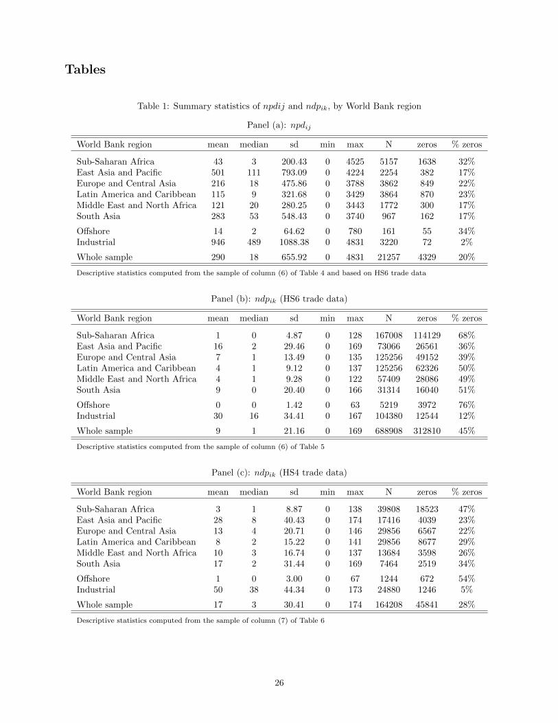
The number of exported products by destination, npdij , counts how many products country i exports to

destination j. As a baseline, we define ‘products’ as HS sub-headings (6 digit HS codes). In the HS 2002

classification that we use, there are 5224 sub-headings. For each ij pair, npdij can therefore theoretically range

between 0 (no trade) and 5224 (country i exports all products to j). Panel (a) of Table 1 presents in-sample

summary statistics for npdij . Overall, the variable varies between 0 and 4831 (the latter being npdUSA−CAN

– the number of HS6 sub-headings exported by the United States to Canada). Disaggregating over World

Bank regions (and excluding ‘Offshore’ and ‘Industrial’ to focus on developing and emerging economies), the

mean of npdij varies between 43 for Sub-Saharan Africa to 501 for East Asia and Pacific. The incidence of

zeros is also highest in Sub-Saharan Africa (32% of observations) and lowest in Asia (together with Middle

East and North Africa). There is, however, considerably less variation across Sub-Saharan African countries

than across countries from other regions.

6

The number of destinations by product, ndpik, counts how many destinations are served by country i’s

exports of product k. In this case, too, the baseline definition of ‘product’ is an HS sub-heading. Panel (b)

of Table 1 presents summary statistics for ndpik. Overall, the variable varies between 0 and 169 (the latter

being the number of Chinese export destinations of HS sub-heading 392690 – ‘Other Articles of Plastics’; HS

sub-heading 830140 – ‘Other locks of Base Metal’; and HS sub-heading 940320 – ‘Other Metal Furniture’).

Again, the disaggregation over World Bank regions reveals relatively low scores for Sub-Saharan Africa (with

an average of 1 destination served by product), and relatively high scores for Asian countries (with an

average of 16 and 9 destinations served by product by East Asia and Pacific and South Asia, respectively).

The incidence of zeros is also highest in Sub-Saharan Africa (68% of observations). The same incidence

ranges between 36% and 51% for other regions.

Panel (c) of Table 1 presents the summary statistics for ndpik computed using HS4 trade data, that is,

defining ‘products’ as HS headings. The number of observations and the percentage of zeros are clearly lower

than for ndpik computed from HS6 trade data. Conversely, in the ij sample the sample size is determined

by the number of exporting and importing countries, not by the level of sectoral disaggregation.

< Table 1 about here >

In the construction of npdij and of ndpik, we rely on mirror trade data to the extent possible because import

data tend to be more complete than export data. We therefore measure exports of country i in product k

using the reported imports of country j in the same product. For the few country-years for which mirror

data is not available, we rely on reported export data.5

3.2 Trade Facilitation Indicators

The sample used for the regressions includes data for 133 countries for which OECD Trade Facilitation

Indicators (TFIs) are available.6 Table 2 presents summary statistics for the variable TFI. This is the simple

average of the country-specific indicators TFIAi , TFIBi , . . . , TFILi .7 The average is unweighted because there

5Mirror data is not available for the years 2010, 2011 and 2012 for the following countries with TFI information: Antiguaand Barbuda, Brunei Darussalam, Cuba, The Gambia, Indonesia, Iran, Kuwait, Mali, Mongolia, Papua New Guinea, Qatar andSuriname.

6The full list of countries by World Bank region group, with information on the date of WTO (GATT, where applicable)membership, is available in Appendix Table A-2.

7We only have information on indicators A-L.

7

is no criterion in the WTO Trade Facilitation Agreement or in its previous drafts to rank different indicators

in terms of their relevance. Since each sub-indicator ranges between 0 and 2, so does TFI. Among developing

and emerging economies, the scores are lowest in Sub-Saharan Africa and highest in Europe and Central

Asia.8 There is however substantial variation within these regions, and especially within Sub-Saharan Africa

(where the best-performing country, Mauritius, has a score of 1.93). The fact that the best performer in

Sub-Saharan Africa (the region with the lowest average of TFI) has the highest score in the data suggests

that a scenario in which all countries in the region move to the best performer’s value is unlikely. We will

take this into account in the simulations of Section 6.


3.3 Econometric model

The TFI data does not vary over time. We therefore estimate cross-sectional regressions for the year 2009.

We choose this year for two reasons. First, this is suggested by Moıse and Sorescu (2013). Second, this

allows us to construct measures for npdij and ndpik that are respectively based on new products and new

destinations, to address endogeneity concerns (see Section 4).9

3.3.1 ij regressions

The ij regressions use, as dependent variable, the number of exported products, npdij . This is a bilateral

measure of trade outcomes. It is therefore natural to employ a gravity framework, with the conditional mean

of the dependent variable expressed as:

E [npdij ∣x1i, ri,gij ,mij ,dj ] = g (x′1iβ + r′iθ + g′ijδ +m′

ijη + d′jγ) (3.1)

In equation (3.1), g(⋅) is a function; x1i is a vector of variables that only vary across exporters i’s; ri is a

vector of exporter-specific region dummies;10 wij is a vector of standard bilateral gravity variables; mij is a

vector of multilateral resistance terms, constructed using the methodology outlined in Baier and Bergstrand

8It is important to note that the latter region does not include industrialized OECD countries – see Table A-2.9The results with all time-varying variables averaged between 2002 and 2010 are very similar to the ones presented here and

are available upon request.10World Bank region dummies are included because in the simulations of Section 6 we average results over such regions.

8

(2009);11 dj is a vector of importer (j)-specific effects; β, θ, δ, η and γ are vectors of coefficients to be

estimated. Appendix Table A-3 provides a description of all the variables, including the data sources.12

Table 3 presents summary statistics for all control variables.


As a first step, we estimate a linear fixed effects model by OLS, with the dependent variable in logs, condi-

tioning on importer-specific effects. In this case, g(⋅) in (3.1) is the identity function. Since the dependent

variable is a count variable, a model for count data is more appropriate (Dennis and Shepherd, 2011; Persson,

2013). Accordingly, we also adopt conditional Poisson and Negative Binomial (NB) Maximum Likelihood

estimations, with the dependent variable in levels (always conditioning on importer-specific effects). In this

case, g(⋅) in (3.1) is the exponential function.13

Appendix Table A-4 presents the in-sample correlations between all variables in the ij sample.

3.3.2 ik regressions

The ik regressions use, as dependent variable, the number of export destinations, ndpik. This measure of

trade outcomes does not have any bilateral dimension, since it varies by exporting country i and by product

k. We express the conditional mean of the dependent variable as:

E [ndpik ∣x2i, ri,hk ] = g (x′2iα + r′iφ + h′kλ) (3.2)

In equation (3.2), g(⋅) is a function; hk is a vector vector of product (k)-specific effects; α, φ and λ are vectors

of coefficients to be estimated. The vectors x2i and x1i differ from one another in the following respects.

x2i, but not x1i, contains the variable Log(remoteness) – a weighted average of partners’ (j’s) world GDP

11In what Head and Mayer (2013) call the ‘structural’ representation of the gravity model, the multilateral resistance termsare exporter and importer specific. In cross-section estimation, it is possible to incorporate these terms as importer and exporterfixed effects a la Feenstra (2003). But since our measure of trade facilitation, TFI, is exporter specific, it is impossible to takethis approach. Instead, given that the multilateral resistance terms enter multiplicatively in the gravity equation, we incorporatethem as a pair or dyadic variable and estimate just one coefficient that measures their combined effect on the number of exportedproducts.

12All variables listed in Appendix Table A-3 are self-explanatory, with the exception of the Market Access Trade Restric-tiveness Index (TRI). The TRI captures the trade policy distortions imposed by the trading partners on i’s export bundle. Itmeasures the uniform tariff equivalent of the partner country tariff and non-tariff barriers (NTB) that would generate the samelevel of i’s export value in a given year. The TRI index is constructed using applied tariffs.

13Both the Poisson and the NB fixed effect estimators are consistent even in short panels. The NB fixed effect estimator yieldsmore efficient estimation in the presence of overdispersion (Cameron and Trivedi, 2013, p. 357). However, it does not allowfor cluster-robust estimation of the variance-covariance matrix. The results are not qualitatively affected by the methodologyadopted.

9

shares, with the inverse distance between i and j as weight (Head and Mayer, 2013). Further, x1i, but not

x2i, contains the variable Log(weighted j’s TFI) – a weighted average of partners’ (j’s) TFI indicators, with

the inverse distance between i and j as weight.14

In this case, too, we present a fixed effect linear specification (OLS with dependent variable in logs) as a

first step. g(⋅) in (3.2) is the identity function in this case. We then adopt conditional Poisson and Negative

Binomial (NB) Maximum Likelihood estimations with the dependent variable in levels. g(⋅) in (3.2) is the

exponential function in this case. We always condition on product-specific effects.

Appendix Table A-5 presents the in-sample correlations between all variables in the ik sample.

4 Results

4.1 ij regressions

The results of the ij regressions are in Table 4. In the OLS regressions, the dependent variable is in logs, while

it is in levels in the Poisson and NB regressions. In both cases, however, the coefficients on the explanatory

variables in logs can be interpreted as elasticities.15


The baseline results are in columns (1), (2) and (6), respectively for OLS, Poisson and NB regressions. The

coefficient on the variable of interest, Log(TFI), is positive and statistically significant in all specifications.

In the specification of column (6), the elasticity is 0.305, implying that a 1% increase in the average trade

facilitation indicator is roughly associated with a 0.3% increase in the number of HS6 products exported by

destination.

The coefficients on the control variables are correctly signed and statistically significant. Although the de-

pendent variable is different, it is useful to compare the distance coefficients with the standard results from

gravity studies. As reported in Table of 4 Head and Mayer (2013), the mean of the distance coefficient

estimated in 159 papers ranges between -0.93 and -1.1, with a standard deviation of 0.40-0.41. The distance

14We are grateful to Richard Baldwin for suggesting the use of this variable.15See Cameron and Trivedi (2013, p. 346). In the OLS regressions, there are fewer observations because all the observations

for which npdij = 0 are dropped. The Poisson and NB regressions drop all observations with npdij = 0 across all destinations,because they do not contribute to the conditional likelihoods.

10

elasticity we obtain is in line with Table 4 of Head and Mayer (2013) for the OLS estimation. In the Poisson

and NB model it is lower, but it is a well-established fact in the literature that the distance coefficient is

lower when using count-data models. Moreover, our result is very similar to the one obtained by Persson

(2013), which is the most comparable study to ours.

We see two possible concerns with the baseline estimations. First, and foremost, we cannot exclude reverse

causation, that is the possibility that trade outcomes affect the incentives to invest in trade facilitation, and

consequently the trade facilitation scores. In the spirit of Freund and Rocha (2011) and Portugal-Perez and

Wilson (2012), we address possible reverse causality using only ‘new products’ (HS sub-headings) in the

construction of the dependent variable. We proceed as follows: when computing how many products country

i exported to country j in 2009, we only include the subset of products for which: (i) there were no exports

from i to j (zero or missing) recorded in any of the years between 2002 and 2007; and (ii) there were positive

exports from i to j recorded in at least one year between 2008 and 2010. Since npdij is, in this case, the count

of new HS6 products that were not traded before 2008, it is less likely to be endogenous to trade facilitation

than the indicator calculated using the set of products traded in 2009.

The use of ‘new products’ has an additional advantage. We do not necessarily exclude products that dropped

from a country’s bilateral export basket during the big trade collapse of 2009. As long as a product that was

not exported in any year between 2002 and 2007 started to be exported in any year before 2008 and 2010, it

counts for the construction of npdij .

The results are in columns (3) and (7) of Table 4. The coefficients are slightly lower than in the baseline

regressions (indicating the possibility of a small downward bias induced by reverse causality), but still positive

and statistically significant.

The second possible concern with the baseline estimations of Table 4 relates to the measurement of trade

facilitation. So far, we have used TFI – the unweighted average of the country-specific OECD Trade Fa-

cilitation Indicators. As an alternative, we have created a trade facilitation indicator based on Principal

Component Analysis (PCA). The results of Poisson estimations are in columns (4) and (5). They are very

similar to the corresponding results of columns (2) and (3).16

16To save space, we do not report NB results with TFI computed using Principal Component Analysis (PCA). They aresimilar to the results in columns (6) and (7) and available upon request.

11

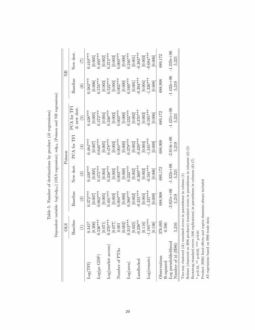
4.2 ik regressions

The results of ik regressions are in Table 5. The structure of the table is similar to that of Table 4.


The coefficient on Log(TFI) is positive and significant in all specifications. The estimated elasticity in column

(6) is 0.383. This implies that a 1% increase in the average trade facilitation indicator is roughly associated

with a 0.38% increase in the number of destinations to which an HS6 product is exported.

In columns (3) and (7) we address possible reverse causality concerns using only ‘new destinations’ in the

computation of the dependent variable. The procedure is very similar in spirit to the one described above

in the case of ij regressions. When computing how many destination countries were served by country i in

exporting product k in 2009, we only include the subset of destinations for which: (i) there were no exports

of product k (zero or missing) recorded in any of the years between 2002 and 2007; (ii) there were positive

exports of product k recorded in at least one year between 2008 and 2010. In this case, therefore, ndpik

becomes the count of new destinations that were not served before 2008.

Also in this case, the use of ‘new destinations’ has the additional advantage that we do not necessarily exclude

destinations that ceased to be served by country i in sector k during the big trade collapse of 2009. As long

as a destination that was not served in any year between 2002 and 2007 started to get served in any year

before 2008 and 2010, it counts for the construction of ndpik.

In the regressions with new destinations, the estimated coefficient on Log(TFI) is slightly larger than the

baseline coefficient, both in the Poisson and in the NB specifications.

In columns (5) and (5) we present the results of the regressions that use a measure of TFI based on Principal

Component Analysis, rather than the simple mean across indicators. Again, the results do not change

significantly.17

17NB results are available upon request.

12

5 Robustness

5.1 Trade margins based on HS4 trade data

The results of ij and ik regressions using trade margins based on HS4 trade data are in Table 6. For

ij regressions, Poisson and NB baseline results should be compared with columns (2) and (6) of Table 4,

respectively. Results with new products (columns (2) and (4)) shoud be compared with columns (3) and (7)

of Table 4. For ik regressions, columns (5) and (7) should be compared with columns (2) and (6) of Table

5, while columns (6) and (8) should be compared with columns (3) and (7) of Table 5. All coefficients on

Log(TFI) are quite similar across comparable regressions. This implies that our results are not affected by

the level of product disaggregation of the data.


5.2 Hummel-Klenow trade margins

In this section, we present econometric estimates using the theory-based ‘Hummels-Klenow extensive margins’

as dependent variables. In the regressions with country pairs, we use the following variable, directly from

Hummels and Klenow (2005):

emij =∑k∈Kij

Xwjk

∑k∈KXwjk(5.1)

In equation (5.1), Kij is the set of goods which country i exports to country j; w is the reference country

that has positive exports to j in all products k (in the empirical implementation, it is the rest of the world);

K is the set of all products; Xwjk are the exports of country w to country j in product k. emij is therefore

the share of those exports to j only in goods k that country i exports in total exports to country j.

In the regressions with country-product observations, we construct a similar measure (not previously used in

the reviewed literature):

emik =∑j∈Jik

Xwjk

∑j∈J Xwjk(5.2)

In equation (5.2), Jik is the set of destinations to which country i exports product k; w is the reference

country that has positive exports of k to all destinations j (in the empirical implementation, it is the rest

13

of the world); J is the set of all destinations; Xwjk are – as in equation (5.1) – the exports of country w

to country j in product k. emik is therefore the share of exports of k only to destinations j that country i

exports to in total exports of product k to all destinations.18

The summary statistics for the Hummels-Klenow extensive margins emij and emik are in Appendix Table

A-6. In the developing world, Hummels-Klenow extensive margins, and therefore export diversification, are

lowest in Sub-Saharan Africa and highest in East Asia and Pacific. From a qualitative standpoint, these

descriptive statistics are in line with the ones presented in Table 1 for npdij and ndpik. In fact, the sample

correlation between npdij and emij is equal to 0.89, while the sample correlation between ndpik and emik is

equal to 0.83.19

Table 7 present the results of ij and ik regressions using, as dependent variable, the Hummels-Klenow

extensive margins emij and emik, respectively. The dependent variable ranges between zero and one. As

suggested by Baum (2008), we use a Generalized Linear Model (GLM) with a logit transformation of the

response variable and the binomial distribution. Odd-numbered columns present baseline results, in which

the respective trade margin is calculated using trade data from 2009. In even-numbered columns we address

concerns related to reverse causality and construct the dependent variable using only the subset of new

products (in the case of emij) or new destinations (in the case of emik).20


In the ij regressions, controlling for country characteristics, partner j dummies, region dummies and bilateral

control variables, the coefficient on Log(TFI) is positive, but it loses statistical significance in column (2). In

the ik regressions, where we control for country characteristics, product k dummies and region dummies, only

the coefficient on Log(TFI) in column (3) is correctly signed and statistically significant. When we use the

definition of the Hummels-Klenow extensive margin emik based on new destinations, this coefficient turns

negative and statistically significant. There is no easy way to explain this counter-intuitive result. It should

be mentioned, however, that the coefficient on Log(TFI) is correctly signed and statistically significant if we

perform the same regression of column (4) of Table 7 using HS4 headings in the construction emik.

18We use the Stata module developed by Ansari (2013) to compute emij and emik.19Sample correlations computed from columns (1) and (3) of Table 7, respectively.20See Section 4.1 for details on the procedure.

14

5.3 World Bank Doing Business indicators

Following, among others, Hoekman and Nicita (2011) and Dennis and Shepherd (2011), we also perform

regressions that use, as proxies for trade facilitation, the ‘Trading across borders’ indicators of the World

Bank Doing Business database. In this database, there are three indicators relevant for our purposes: number

of documents to export;21 number of days required to export;22 and cost to export (US$ per container).23

To increase comparability with the results that use the OECD TFIs, we transform these variables as follows.

First, we compute their inverse. Then, we rescale them between 0 (least facilitation) and 2 (most facilitation).

Appendix Table A-7 presents the in-sample correlations among these variables, and the correlations between

these variables and TFI.

The results are in Table 8. All the coefficients on DB docs, DB cost and DB time are consistently positive

across all specifications, both in the ij and in the ik regressions. It should be noted that ij regressions use

the same set of explanatory variables as Table 4 and ik regressions use the same set of explanatory variables

as Table 5.


5.4 The elusive quest for heterogeneous effects

Beyond the central results of Section 4, we also investigate possible heterogeneity in the impact of trade

facilitation on the extensive margins of trade. An important potential source of heterogeneity is between

country pairs that have a PTA in place and country pairs that do not have one. There is ample evidence

that most PTAs include trade facilitation provisions (see for instance Neufeld, 2014). Maur (2011) argues

that in areas such as product standards and technical regulations, trade facilitation through policies such

as harmonization between PTA members has the potential to introduce discrimination vis-a-vis excluded

countries. Conversely, aspects of trade facilitation such as transparency and simplification of rules and

procedures (the narrow definition of trade facilitation that we use in this paper and that is reflected in the

21The total number of documents required per shipment to export goods. Documents required for clearance by governmentministries, customs authorities, port and container terminal authorities, health and technical control agencies and banks aretaken into account.

22The time necessary to comply with all procedures required to export goods.23The cost associated with all procedures required to export goods. It includes the costs for documents, administrative fees

for customs clearance and technical control, customs broker fees, terminal handling charges and inland transport.

15

OECD TFIs), should be non-discriminatory in nature and therefore benefit all trading partners equally. If

this is the case, one should not expect any heterogeneous effect of exporter’s trade facilitation on the extensive

margin of bilateral trade across importers with a PTA with the exporter and importers without.

To test this prediction, we augment the ij regressions with an interaction term between the PTA dummy and

Log(TFI). We do not obtain any consistent pattern in the results. In most regressions, the marginal effect

when the PTA dummy is equal to one is not statistically different from the marginal effect when the PTA

dummy is equal to zero. The evidence that an exporting country’s trade facilitation does not have a higher

impact on the bilateral extensive margin with importers with which it has a PTA provides indirect support

for the idea that the trade facilitation provisions captured by the OECD TFIs (and disciplined by the WTO

Trade Facilitation Agreement) are non-discriminatory.

In a similar way, we investigate the effects of having a common border (without any significant result) or a

common language. Although obtaining significant results in a few instances, indicating that trade facilitation

is even more important if the trading partners have different languages, we do not find consistent results

across all specifications.24

One might be concerned that our results might be driven by developed countries only. To rule this out,

we split the ij sample in four subsamples: DD (both exporter i and importer j are developed);25 DG (i is

developed, j is developing); GD (i is developing, j is developed); GG (both i and j are developing). As

shown in Table 9, each of these subsample covers approximately one quarter of the ij dataset. Although

varying in magnitude across different specifications, the results are qualitatively similar across sub-samples.

We therefore reject the hypothesis that our results are driven by developed countries.


We further check whether the effect of trade facilitation on the extensive margins differs between final and

intermediate products. Yi (2003) developes a model in which trade costs hamper vertically-specialized trade

(i.e. trade along supply chains) relatively more than trade in final products.26 Martinez-Zarzoso and Marquez-

24The results are available upon request.25We consider ‘developed’ countries classified by the World Bank as High-income or Upper-middle-income economies. Low-

income and Lower-middle-income economies are considered ‘developing’.26Yi’s model shows the magnifying trade effects of tariff reductions when vertically specialized goods cross multiple borders

while they are being produced. He argues that reductions in transportation costs and trade reforms more general than tariffliberalization also have a magnifying effect on trade. Ferrantino (2012) makes the link with trade facilitation explicit. He argues

16

Ramos (2008) show that improvements in the Doing Business indicators ‘Number of days’ and ‘Document

required’ to export/import have a relatively larger effect on technology-intensive goods and on differentiated

products, as opposed to homogeneous ones. Marti et al. (2014) argue that improvements in the LPI have an

effect which is larger for goods that are relatively more complex to transport. In a more direct test of Yi’s

hypothesis, Saslavsky and Shepherd (2012) show that trade in parts and components – which they assume

takes place largely within production networks – is more sensitive to improvements in logistics performance

than trade in final goods. These papers focus on the intensive margin of trade (bilateral trade value in a gravity

framework). As discussed in Section 2, Persson (2013) applies similar ideas to the extensive margins of trade.

She does not explicitly consider trade in intermediate products as her focus is on product differentiation. She

finds that trade facilitation has a higher extensive margin impact on trade in differentiated products than on

trade in homogenous products.

In the spirit of this literature, we test for heterogeneous effects on the extensive margins of trade between

intermediate and non-intermediate and products. We use two alternative definitions of intermediate products,

a narrow one and a broad one. The narrow definition, adopted by WTO (2011), includes the HS sub-headings

corresponding to codes 42 and 53 of the Broad Economic Categories (BEC) classification, supplemented

with unfinished textile products in HS chapters 50-63. The broad definition includes the HS sub-headings

corresponding to the intermediate goods of the BEC classification.

As a first step, we estimate the ij regressions in two sub-samples: one in which the dependent variable

is computed across the subset of intermediate products; one in which the dependent variable is computed

across the subset of all other products. We are not able to find any significant difference between estimated

coefficients across these specifications. To test this result further, in the ik sample we augment the regressions

with an interaction term between a dummy equal to one if the product is intermediate and the Log(TFI)

variable. We do not find the coefficient of this interaction term to be significant in most specifications.27

This leads us to conclude that the effect of trade facilitation on the extensive margin does not differ between

intermediate and final products.

that NTMs and trade facilitation can be compared using a common metric. Efforts to reduce NTMs and efforts to increasetrade facilitation should both have larger effects on trade in complex supply chains that on trade in simple supply chains. Seealso U.S. Chamber of Commerce (2014) and UNECA (2013) for less formal expositions, respectively by the business communityand by an international organization, of the idea that trade facilitation should matter most for intermediate goods trade.

27The results are available upon request.

17

6 Simulation results

In this section, we present the results of counterfactual analysis aimed at providing insights into the economic

significance of our results. We estimate the percentage increase in the number of export destinations and in

the number of exported products under two different scenarios. As shown in the ‘sd’ column of Table 2, there

is wide variation in TFI scores across countries belonging to the same geographical region. This suggests that

a scenario involving convergence to the top regional performer would be very unrealistic. Such a scenario is,

therefore, discarded a priori. Instead we consider two realistic scenarios. The first scenario is one in which

each country with a TFI score below the median of the geographical region it belongs to increases its TFI to

the regional median. The second scenario considers an increase to the global median.

It is important to note that results of counterfactual analysis have to be taken cautiously. First, because they

are only as good as the underlying econometric model. Although we have taken care in addressing omitted

variable and reverse causality biases, we cannot control for every possible country-specific variable correlated

with trade facilitation and we cannot completely exclude the endogenous co-determination of trade outcomes

and trade facilitation infrastructure. Second, the counter-factual analysis does not take into account that

regional (global) median values would be affected by changes in trade facilitation occurring in all countries

in the region (world).

With these caveats in mind, the baseline results, grouped by region, are presented in Table 10 for ij regressions

and Table 11 for ik regressions. To remain on the conservative side, we have chosen to base the simulations

on the Negative Binomial (NB) results, which generally yield smaller estimated coefficients on Log(TFI) than

the coefficients of Poisson regressions.28

For ease of interpretation, it is useful to keep in mind that the entries in tables 10 and 11 represent the

percentage change in the variable of interest (respectively, npdij and ndpik) that, based on the estimated

regression coefficients, are predicted if country i moves from below the regional (global) median to the relevant

median. The results are then averaged across regions. All countries at, or above, the relevant median are

dropped from the calculation of the regional average percentage increase in the trade margin. If, say, in a

given region there are 16 countries, 8 of which are below the regional median and 15 below the global median,

28The simulation results using the coefficients from Poisson regressions are available upon request.

18

the results under the regional median scenario are averaged over the 8 bottom countries in terms of TFI,

while the results under the global median scenario are averaged over all countries with the exclusion of the

top regional performer.

Tables 10 and 11 have two panels each. In the upper panel, we present results based on regressions using HS6

trade data. In the lower panel, we present results based on regressions using HS4 trade data. We use both

the ‘baseline’ NB and the NB specifications with new products and new destinations. Since the estimates

obtained in the latter specifications address the issue of reverse causality, we take them as our preferred

results. We therefore discuss only the results of even-numbered columns.

< Tables 10 and 11 about here >

As expected, the estimated gains in terms of number of products exported by destination (npdij) are quite

similar in panels (a) and (b) of Table 10 (the correlation between npdij computed from HS6 trade data and

npdij computed from HS4 trade data is 0.98), but also in panels (a) and (b) of Table 11. The percentage gains

range from 4.1% in the case of South Asia (HS4 data, both scenarios) to 15.7% in the case of Sub-Saharan

Africa (HS6 data, global median scenario). It is apparent from the table that the gains are largest in two

regions, namely Sub-Saharan Africa and Latin America and the Caribbean.

In the case of the number of export destinations by product (ndpik), the estimated gains range from 7.2%

for South Asia (regional median scenario, HS4 regressions) to 27.9% for Sub-Saharan Africa (global median

scenario, HS6 regressions). In this case, too, the gains are largest in Sub-Saharan Africa and Latin America

and the Caribbean.

7 Conclusions

This is the first paper to focus exclusively on, and to provide detailed estimates of, the prospective effect of

the WTO Trade Facilitation Agreement on export diversification, as measured by the extensive margins of

trade. We do so by using direct measures of trade facilitation that map into the obligations of the agreement,

namely, the OECD Trade Facilitation Indicators. We explore a variety of measures of the extensive margins

of trade – the number of products a country exports to a given destination (npdij), the number of destinations

19

to which a country exports a given product (ndpik), the Hummels-Klenow measure of the bilateral extensive

margin (emij) and a similar measure of the country-product extensive margin (emik) that has not previously

been explored in the literature.

The estimation results are convincing, with the coefficient on the trade facilitation variable being positive

and statistically significant across almost all specifications. Using these estimates, we simulate the impact

of implementing the agreement on developing countries’ extensive margin of trade. Implementation of the

agreement is measured using two alternative realistic scenarios – convergence to the regional median and

convergence to the global median. Developing countries are likely to experience a substantial increase in the

number of products exported and of destination markets. For Sub-Saharan African countries, our simulations

suggest they could see an increase of up to 15.7% in the number of products exported by destination and an

increase of up to 27.9% in the number of export destinations by product. For countries in Latin America and

the Caribbean, our simulations suggest they could see an increase of up to 12.2% in the number of products

exported by destination and an increase of up to 21.7% in the number of export destinations by product. For

the reasons outlined in Section 6, these numbers have to be treated with caution. Nonetheless, they imply

potentially sizeable impacts of the Trade Faciliation Agreement on extensive margins of export, and therefore

on export diversification.

We see three potential avenues for further research. First, the analysis could be conducted at the level of

specific TFI indicators. Such analysis would shed light on which provisions of the WTO Trade Facilitation

Agreement have the most effect on the extensive margins of trade. Second, simulations could be based on

actual implementation schedules which will have to be notified by WTO members. Third, research should

focus on the effect of trade facilitation on trade margins computed from firm-level, as opposed to sector-level

data.

Finally, we emphasize that we make no claim about the welfare effects of implementing the WTO Trade

Facilitation Agreement. This would require us to estimate not only the benefits but also the costs of imple-

menting the agreement. Notwithstanding this qualification, we know from the available literature that the

costs of implementation of trade facilitation initiatives are relatively small (OECD, 2009; UNECA, 2013). At

the same time, our estimations do not capture several other potential benefits of the agreement. A proper

20

welfare analysis would also factor in the value of locking in commitments in a multilateral agreement and

other positive spillovers, such as, for instance, the reduction in the extent of rent-seeking behaviour or the

environmental benefit of lower fuel consumption from shorter waiting times at the border. These topics

need to be investigated further to get a more comprehensive understanding of the effects of the WTO Trade

Facilitation Agreement.

21

References

Anderson, J. E., and E. van Wincoop, 2004, “Trade Costs,” Journal of Economic Literature, 42, 691–751.

Ansari, M. R., 2013, “HUMMELS: Stata module to compute intensive and extensive trade margins,” Statis-

tical Software Components, Boston College Department of Economics.

Arvis, J.-F., Y. Duval, B. Shepherd, and C. Utoktham, 2013, “Trade costs in the developing world: 1995-

2010,” World Bank Policy Research Working Paper No. 6309.

Baier, S. L., and J. H. Bergstrand, 2009, “Bonus vetus OLS: A simple method for approximating international

trade-cost effects using the gravity equation,” Journal of International Economics, 77, 77–85.

Baum, C. F., 2008, “Stata tip 63: Modeling proportions,” The Stata Journal, 8, 299–303.

Cameron, A. C., and P. K. Trivedi, 2013, Regression analysis of count data, Econometric Society monograph

No. 53, Cambridge University Press, New York, second edn.

Chen, N., and D. Novy, 2009, “International Trade Integration: A Disaggregated Approach,” CEP Discussion

Paper No. 0908, Centre for Economic Performance, LSE.

Dennis, A., and B. Shepherd, 2011, “Trade Facilitation and Export Diversification,” The World Economy,

34, 101–122.

Djankov, S., C. Freund, and C. S. Pham, 2010, “Trading on time,” The Review of Economics and Statistics,

92, 166–173.

Feenstra, R. C., 2003, Advanced international trade: theory and evidence, Princeton University Press, Prince-

ton, NJ.

Feenstra, R. C., and H. Ma, 2014, “Trade Facilitation and the Extensive Margin of Exports,” Japanese

Economic Review, 65, 158–177.

Fernandes, A. M., and R. Hillberry, 2014, “Customs reform and trade growth: Evidence from Albania,”

Presented at the Third Annual WTO/IMF/World Bank Trade Workshop, Washington, D.C., 7 November.

22

Ferrantino, M. J., 2012, “Using Supply Chain Analysis to Examine the Costs of Non-Tariff Measures (NTMs)

and the Benefits of Trade Facilitation,” WTO Staff Working Paper No. ERSD-2012-02.

Freund, C., and N. Rocha, 2011, “What Constrains Africa’s Exports?,” World Bank Economic Review, 25,

361–386.

Hausman, W. H., H. L. Lee, and U. Subramanian, 2013, “The Impact of Logistics Performance on Trade,”

Production and Operations Management, 22, 236–252.

Head, K., and T. Mayer, 2013, “Gravity equations: Workhorse, toolkit, and cookbook,” in E. Helpman, K.

Rogoff, and G. Gopinath (ed.), Handbook of International Economics, 4: 131-195, Elsevier, Oxford and

Amsterdam.

Head, K., T. Mayer, and J. Ries, 2010, “The erosion of colonial trade linkages after independence,” Journal

of International Economics, 81, 1–14.

Hoekman, B., and A. Nicita, 2011, “Trade Policy, Trade Costs, and Developing Country Trade,” World

Development, 39, 2069–2079.

Hufbauer, G., J. Schott, C. Cimino, and J. Muir, 2013, “Payoff from the World trade agenda,” Report to the

ICC Research Foundation, Peterson Institute for International Economics.

Hummels, D., and P. J. Klenow, 2005, “The Variety and Quality of a Nation’s Exports,” American Economic

Review, 95, 704–723.

Hummels, D. L., and G. Schaur, 2013, “Time as a Trade Barrier,” American Economic Review, 103, 2935–

2959.

Iwanow, T., and C. Kirkpatrick, 2009, “Trade Facilitation and Manufactured Exports: Is Africa Different?,”

World Development, 37, 1039 – 1050.

Kee, H. L., A. Nicita, and M. Olarreaga, 2009, “Estimating Trade Restrictiveness Indices,” Economic Journal,

119, 172–199.

23

Marti, L., R. Puertas, and L. Garcıa, 2014, “Relevance of trade facilitation in emerging countries’ exports,”

The Journal of International Trade & Economic Development, 23, 202–222.

Martinez-Zarzoso, I., and L. Marquez-Ramos, 2008, “The Effect of Trade Facilitation on Sectoral Trade,”

The B.E. Journal of Economic Analysis & Policy, 8, 1–46.

Maur, J. C., 2011, “Trade facilitation,” in J.-P. Chauffour, and J. C. Maur (ed.), Preferential trade Agreement

Policies for Development, The World Bank, Washington, D.C.

Melitz, M. J., 2003, “The Impact of Trade on Intra-Industry Reallocations and Aggregate Industry Produc-

tivity,” Econometrica, 71, 1695–1725.

Moıse, E., T. Orliac, and P. Minor, 2011, “Trade Facilitation Indicators: The Impact on Trade Costs,” OECD

Trade Policy Paper No. 118.

Moıse, E., and S. Sorescu, 2013, “Trade Facilitation Indicators: The Potential Impact of Trade Facilitation

on Developing Countries’ Trade,” OECD Trade Policy Paper No. 144.

Neufeld, N., 2014, “Trade Facilitation Provisions in Regional Trade Agreements – Traits and Trends,” WTO

Staff Working Paper No. ERSD-2014-01.

Nordas, H. K., E. Pinali, and M. Geloso Grosso, 2006, “Logistics and Time as a Trade Barrier,” OECD Trade

Policy Paper No. 35.

Novy, D., 2013, “Gravity Redux: Measuring International Trade Costs With Panel Data,” Economic Inquiry,

51, 101–121.

Organization for Economic Co-operation and Development (OECD), 2009, Overcoming Border Bottlenecks:

The Costs and Benefits of Trade Facilitation, OECD, Paris.

Persson, M., 2013, “Trade facilitation and the extensive margin,” The Journal of International Trade &

Economic Development, 22, 658–693.

Portugal-Perez, A., and J. S. Wilson, 2012, “Export Performance and Trade Facilitation Reform: Hard and

Soft Infrastructure,” World Development, 40, 1295 – 1307.

24

Saslavsky, D., and B. Shepherd, 2012, “Facilitating international production networks : the role of trade

logistics,” Policy Research Working Paper No. 6224, The World Bank.

United Nations Economic Commission for Africa (UNECA), 2013, Trade Facilitation from an African Per-

spective, Economic Commission for Africa, Addis Ababa, Ethiopia.

U.S. Chamber of Commerce, 2014, “Global Supply Chain, Customs and

Trade Facilitation,” available at https://www.uschamber.com/issue-brief/

global-supply-chain-customs-and-trade-facilitation. [Accessed 6 October 2014].

Volpe Martincus, C., J. Carballo, and A. Graziano, 2013, “Customs as Doorkeepers: What Are Their Effects

on International Trade?,” available at http://www.usitc.gov/research_and_analysis/documents/

Customs_as-Doorkeepers-What_Are_Their_Effects_on_International_Trade.pdf.

World Trade Organization (WTO), 2011, World Trade Report 2011. The WTO and preferential trade agree-

ments: From co-existence to coherence, World Trade Organization, Geneva.

Yi, K.-M., 2003, “Can Vertical Specialization Explain the Growth of World Trade?,” Journal of Political

Economy, 111, pp. 52–102.

Zaki, C., 2014, “An empirical assessment of the trade facilitation initiative: econometric evidence and global

economic effects,” World Trade Review, 13, 103–130.

25

https://www.uschamber.com/issue-brief/global-supply-chain-customs-and-trade-facilitation

https://www.uschamber.com/issue-brief/global-supply-chain-customs-and-trade-facilitation

http://www.usitc.gov/research_and_analysis/documents/Customs_as-Doorkeepers-What_Are_Their_Effects_on_International_Trade.pdf

http://www.usitc.gov/research_and_analysis/documents/Customs_as-Doorkeepers-What_Are_Their_Effects_on_International_Trade.pdf

Tables

Table 1: Summary statistics of npdij and ndpik, by World Bank region

Panel (a): npdij

World Bank region mean median sd min max N zeros % zeros

Sub-Saharan Africa 43 3 200.43 0 4525 5157 1638 32%East Asia and Pacific 501 111 793.09 0 4224 2254 382 17%Europe and Central Asia 216 18 475.86 0 3788 3862 849 22%Latin America and Caribbean 115 9 321.68 0 3429 3864 870 23%Middle East and North Africa 121 20 280.25 0 3443 1772 300 17%South Asia 283 53 548.43 0 3740 967 162 17%

Offshore 14 2 64.62 0 780 161 55 34%Industrial 946 489 1088.38 0 4831 3220 72 2%

Whole sample 290 18 655.92 0 4831 21257 4329 20%

Descriptive statistics computed from the sample of column (6) of Table 4 and based on HS6 trade data

Panel (b): ndpik (HS6 trade data)




Whole sample 9 1 21.16 0 169 688908 312810 45%

Descriptive statistics computed from the sample of column (6) of Table 5

Panel (c): ndpik (HS4 trade data)




Whole sample 17 3 30.41 0 174 164208 45841 28%


26

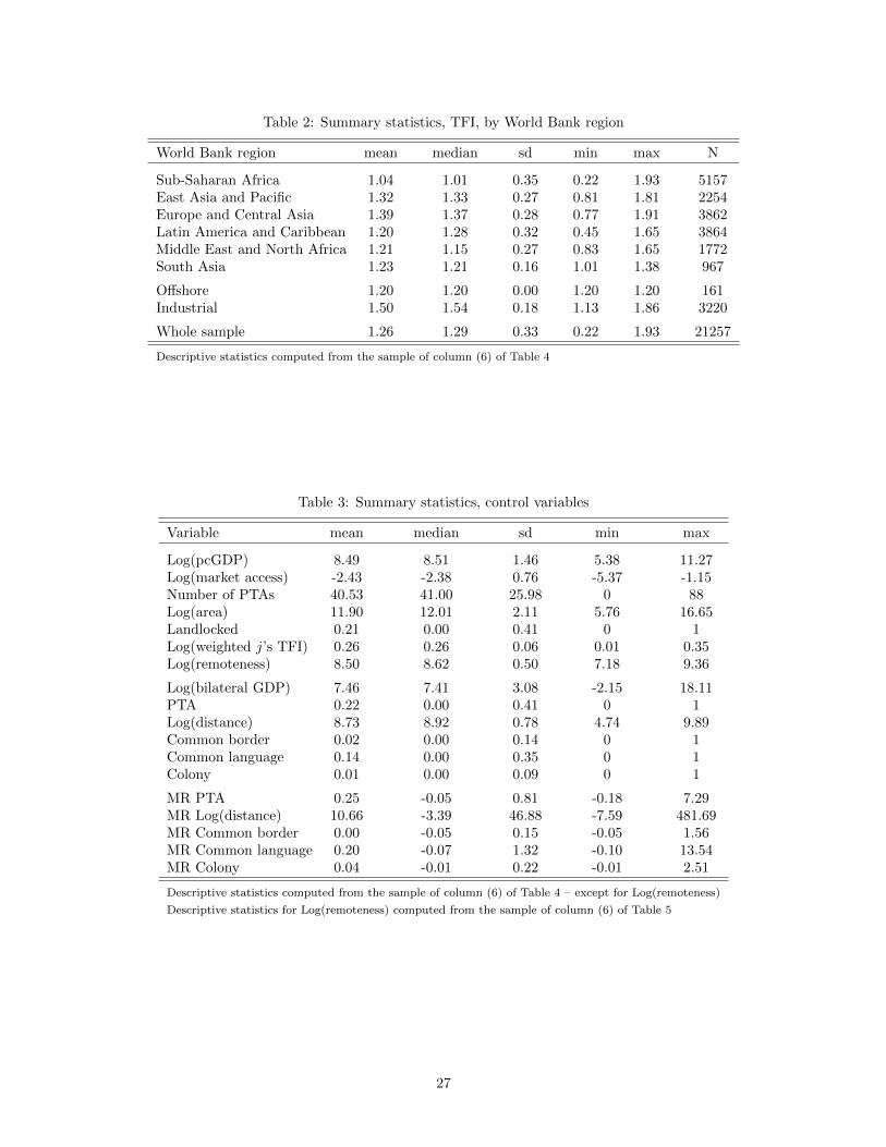
Table 2: Summary statistics, TFI, by World Bank region

World Bank region mean median sd min max N

Sub-Saharan Africa 1.04 1.01 0.35 0.22 1.93 5157East Asia and Pacific 1.32 1.33 0.27 0.81 1.81 2254Europe and Central Asia 1.39 1.37 0.28 0.77 1.91 3862Latin America and Caribbean 1.20 1.28 0.32 0.45 1.65 3864Middle East and North Africa 1.21 1.15 0.27 0.83 1.65 1772South Asia 1.23 1.21 0.16 1.01 1.38 967

Offshore 1.20 1.20 0.00 1.20 1.20 161Industrial 1.50 1.54 0.18 1.13 1.86 3220

Whole sample 1.26 1.29 0.33 0.22 1.93 21257


Table 3: Summary statistics, control variables

Variable mean kk median kk sd kk min kk max

Log(pcGDP) 8.49 8.51 1.46 5.38 11.27Log(market access) -2.43 -2.38 0.76 -5.37 -1.15Number of PTAs 40.53 41.00 25.98 0 88Log(area) 11.90 12.01 2.11 5.76 16.65Landlocked 0.21 0.00 0.41 0 1Log(weighted j’s TFI) 0.26 0.26 0.06 0.01 0.35Log(remoteness) 8.50 8.62 0.50 7.18 9.36

Log(bilateral GDP) 7.46 7.41 3.08 -2.15 18.11PTA 0.22 0.00 0.41 0 1Log(distance) 8.73 8.92 0.78 4.74 9.89Common border 0.02 0.00 0.14 0 1Common language 0.14 0.00 0.35 0 1Colony 0.01 0.00 0.09 0 1

MR PTA 0.25 -0.05 0.81 -0.18 7.29MR Log(distance) 10.66 -3.39 46.88 -7.59 481.69MR Common border 0.00 -0.05 0.15 -0.05 1.56MR Common language 0.20 -0.07 1.32 -0.10 13.54MR Colony 0.04 -0.01 0.22 -0.01 2.51

Descriptive statistics computed from the sample of column (6) of Table 4 – except for Log(remoteness)

Descriptive statistics for Log(remoteness) computed from the sample of column (6) of Table 5

27

Tab

le4:

Nu

mb

erof

pro

du

cts

by

des

tin

ati

on

(ij

regre

ssio

ns)

Dep

enden

tva

riable

:log(n

pdij)(

OL

Sre

gre

ssio

n);

npdij

(Pois

son

and

NB

regre

ssio

ns)

OL

SP

ois

son

NB

Bas

elin

eB

ase

lin

eN

ewH

S6

PC

Afo

rT

FI

PC

Afo

rT

FI

Base

lin

eN

ewH

S6

&n

ewH

S6

(1)

(2)

(3)

(4)

(5)

(6)

(7)

Log

(TF

I)0.

290*

**0.5

49***

0.3

46***

0.6

08***

0.3

19***

0.3

05***

0.2

30***

[0.0

38]

[0.0

57]

[0.0

78]

[0.0

64]

[0.0

81]

[0.0

24]

[0.0

28]

Log

(pc

GD

P)

0.11

3***

0.0

97***

0.0

88***

0.0

93***

0.0

90***

0.2

18***

0.1

02***

[0.0

18]

[0.0

25]

[0.0

30]

[0.0

25]

[0.0

30]

[0.0

17]

[0.0

19]

Log

(mar

ket

acce

ss)

0.43

3***

0.4

01***

0.3

04***

0.3

94***

0.3

04***

0.3

20***

0.2

37***

[0.0

13]

[0.0

18]

[0.0

21]

[0.0

18]

[0.0

21]

[0.0

10]

[0.0

09]

Nu

mb

erof

PT

As

-0.0

02**

*0.0

02***

0.0

01*

0.0

02**

0.0

01

0.0

03***

0.0

02***

[0.0

01]

[0.0

01]

[0.0

01]

[0.0

01]

[0.0

01]

[0.0

00]

[0.0

00]

Log

(are

a)-0

.058

***

-0.0

48***

-0.0

21**

-0.0

47***

-0.0

20**

0.0

40***

0.0

15**

[0.0

07]

[0.0

09]

[0.0

09]

[0.0

09]

[0.0

09]

[0.0

08]

[0.0

07]

Lan

dlo

cked

-0.2

48**

*0.0

11

-0.1

56***

0.0

15

-0.1

55***

-0.0

78***

-0.2

00***

[0.0

24]

[0.0

28]

[0.0

27]

[0.0

28]

[0.0

27]

[0.0

23]

[0.0

12]

Log

(wei

ghte

dj’

sT

FI)

4.71

8***

1.6

57***

1.0

82***

1.7

96***

1.0

96***

0.7

18***

0.7

08***

[0.2

91]

[0.4

32]

[0.3

39]

[0.4

31]

[0.3

43]

[0.2

31]

[0.1

86]

Log

(bil

ater

alG

DP

)0.

788*

**0.7

35***

0.4

76***

0.7

30***

0.4

75***

0.3

97***

0.3

66***

[0.0

14]

[0.0

21]

[0.0

27]

[0.0

21]

[0.0

26]

[0.0

22]

[0.0

15]

PT

A0.

115*

**0.0

54

0.0

04

0.0

51

0.0

05

0.0

50

-0.0

02

[0.0

41]

[0.0

39]

[0.0

33]

[0.0

39]

[0.0

33]

[0.0

30]

[0.0

29]

Log

(dis

tan

ce)

-0.9

31**

*-0

.598***

-0.4

31***

-0.6

00***

-0.4

32***

-0.4

77***

-0.2

93***

[0.0

36]

[0.0

41]

[0.0

35]

[0.0

41]

[0.0

35]

[0.0

30]

[0.0

28]

Com

mon

bor

der

0.48

2***

-0.0

36

-0.1

10

-0.0

33

-0.1

09

-0.1

84***

-0.5

26***

[0.1

16]

[0.0

86]

[0.1

03]

[0.0

85]

[0.1

03]

[0.0

66]

[0.1

33]

Com

mon

lan

guag

e0.

757*

**0.3

91***

0.4

22***

0.3

83***

0.4

20***

0.3

65***

0.3

06***

[0.0

51]

[0.0

55]

[0.0

46]

[0.0

55]

[0.0

46]

[0.0

40]

[0.0

40]

Col

ony

0.77

7***

0.5

82***

0.3

71***

0.5

89***

0.3

74***

0.3

37***

0.2

59**

[0.1

35]

[0.1

06]

[0.1

08]

[0.1

06]

[0.1

08]

[0.1

02]

[0.1

26]

Ob

serv

atio

ns

16,9

2821,2

57

21,3

88

21,2

57

21,3

88

21,2

57

21,3

88

R-s

qu

ared

0.74

0L

ogp

seu

dol

ikel

ihood

-1.3

49e+

06

-784586

-1.3

45e+

06

-784897

-97952

-99089

Nu

mb

erof

id(j

’s)

162

162

163

162

163

162

163

Rob

ust

(clu

ster

edon

part

ner

j)st

an

dard

erro

rsin

pare

nth

eses

inco

lum

ns

(1)-

(5)

Boots

trap

stan

dard

erro

rs(1

00

rep

lica

tion

s)in

pare

nth

eses

inco

lum

ns

(6)-

(7)

*p<0.1

0,

**

p<0.0

5,

***

p<0.0

1

Part

ner

jfi

xed

effec

ts,

regio

nd

um

mie

san

dM

Rco

ntr

ols

alw

ays

incl

ud

ed

All

regre

ssio

ns

base

don

HS

6tr

ad

ed

ata

28

Tab

le5:

Nu

mb

erof

des

tin

ati

on

sby

pro

du

ct(ik

regre

ssio

ns)

Dep

enden

tva

riable

:log(n

dpik)(

OL

Sre

gre

ssio

n);

ndpik

(Pois

son

and

NB

regre

ssio

ns)

OL

SP

ois

son

NB

Bas

elin

eB

ase

lin

eN

ewd

est.

PC

Afo

rT

FI

PC

Afo

rT

FI

Base

lin

eN

ewd

est.

&n

ewd

est.

(1)

(2)

(3)

(4)

(5)

(6)

(7)

Log

(TF

I)0.

345*

0.3

72***

0.4

39***

0.4

84***

0.4

38***

0.3

83***

0.4

10***

[0.2

00]

[0.0

07]

[0.0

05]

[0.0

07]

[0.0

05]

[0.0

06]

[0.0

05]

Log

(pc

GD

P)

0.53

6***

0.6

62***

0.4

75***

0.6

46***

0.4

72*

**

0.5

76***

0.4

93***

[0.0

71]

[0.0

05]

[0.0

04]

[0.0

05]

[0.0

04]

[0.0

03]

[0.0

02]

Log

(mar

ket

acce

ss)

0.37

0***

0.4

91***

0.3

38***

0.4

78***

0.3

36***

0.5

22***

0.3

74***

[0.0

77]

[0.0

03]

[0.0

03]

[0.0

03]

[0.0

03]

[0.0

03]

[0.0

03]

Nu

mb

erof

PT

As

0.00

10.0

04***

0.0

03***

0.0

04***

0.0

03*

**

0.0

02***

0.0

03***

[0.0

02]

[0.0

00]

[0.0

00]

[0.0

00]

[0.0

00]

[0.0

00]

[0.0

00]

Log

(are

a)0.

313*

**0.3

80***

0.2

32***

0.3

79***

0.2

32***

0.3

49***

0.2

46***

[0.0

25]

[0.0

02]

[0.0

02]

[0.0

02]

[0.0

02]

[0.0

01]

[0.0

01]

Lan

dlo

cked

-0.2

38**

-0.3

31***

-0.3

69***

-0.3

29***

-0.3

70***

-0.3

94***

-0.3

83***

[0.1

16]

[0.0

04]

[0.0

03]

[0.0

04]

[0.0

03]

[0.0

04]

[0.0

03]

Log

(rem

ote)

-1.1

85**

*-1

.237***

-0.5

91***

-1.2

45***

-0.5

95***

-1.3

26***

-0.6

84***

[0.1

36]

[0.0

09]

[0.0

06]

[0.0

09]

[0.0

06]

[0.0

08]

[0.0

06]

Ob

serv

atio

ns

376,

095

688,9

08

689,1

72

688,9

08

689,1

72

688,9

08

689,1

72

R-s

qu

ared

0.59

0L

ogp

seu

dol

ikel

ihood

-2.6

21e+

06

-1.4

22e+

06

-2.6

14e+

06

-1.4

21e+

06

-1.4

32e+

06

-1.2

35e+

06

Nu

mb

erof

id(H

S6)

5,21

65,2

19

5,2

21

5,2

19

5,2

21

5,2

19

5,2

21

Tw

o-w

ay

clu

ster

ed(ik)

stan

dard

erro

rsin

pare

nth

eses

inco

lum

n(1

)

Rob

ust

(clu

ster

edon

HS

6p

rod

uct

s)st

an

dard

erro

rsin

pare

nth

eses

inco

lum

ns

(2)-

(5)

Boots

trap

stan

dard

erro

rs(1

00

rep

lica

tion

s)in

pare

nth

eses

inco

lum

ns

(6)-

(7)

*p<0.1

0,

**

p<0.0

5,

***

p<0.0

1

Pro

du

ct(H

S6)

fixed

effec

tsan

dre

gio

nd

um

mie

salw

ays

incl

ud

ed

All

regre

ssio

ns

base

don

HS

6tr

ad

ed

ata

29

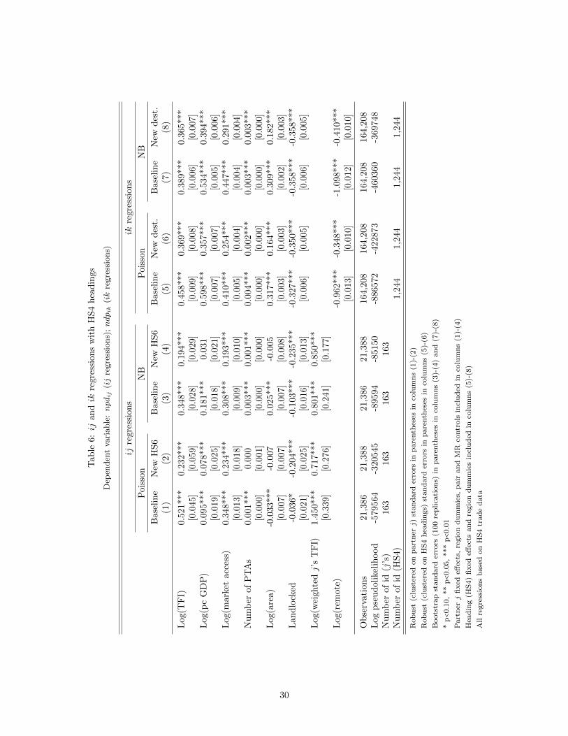
Tab

le6:ij

an

dik

regre

ssio

ns

wit

hH

S4

hea

din

gs

Dep

enden

tva

riable

:npdij

(ij

regre

ssio

ns)

;ndpik

(ik

regre

ssio

ns)

ijre

gre

ssio

ns

ikre

gre

ssio

ns

Poi

sson

NB

Pois

son

NB

Bas

elin

eN

ewH

S6

Base

lin

eN

ewH

S6

Base

lin

eN

ewd

est.

Base

lin

eN

ewd

est.

(1)

(2)

(3)

(4)

(5)

(6)

(7)

(8)

Log

(TF

I)0.

521*

**0.

232***

0.3

48***

0.1

94***

0.4

58***

0.3

69***

0.3

89***

0.3

65***

[0.0

45]

[0.0

59]

[0.0

28]

[0.0

29]

[0.0

09]

[0.0

08]

[0.0

06]

[0.0

07]

Log

(pc

GD

P)

0.09

5***

0.0

78***

0.1

81***

0.0

31

0.5

98***

0.3

57***

0.5

34***

0.3

94***

[0.0

19]

[0.0

25]

[0.0

18]

[0.0

21]

[0.0

07]

[0.0

07]

[0.0

05]

[0.0

06]

Log

(mar

ket

acce

ss)

0.34

8***

0.234***

0.3

08***

0.1

93***

0.4

10***

0.2

54***

0.4

47***

0.2

91***

[0.0

13]

[0.0

18]

[0.0

09]

[0.0

10]

[0.0

05]

[0.0

04]

[0.0

04]

[0.0

04]

Nu

mb

erof

PT

As

0.00

1***

0.0

00

0.0

03***

0.0

01***

0.0

04***

0.0

02***

0.0

03***

0.0

03***

[0.0

00]

[0.0

01]

[0.0

00]

[0.0

00]

[0.0

00]

[0.0

00]

[0.0

00]

[0.0

00]

Log

(are

a)-0

.033

***

-0.0

07

0.0

25***

-0.0

05

0.3

17***

0.1

64***

0.3

09***

0.1

82***

[0.0

07]

[0.0

07]

[0.0

07]

[0.0

08]

[0.0

03]

[0.0

03]

[0.0

02]

[0.0

03]

Lan

dlo

cked

-0.0

36*

-0.2

04***

-0.1

03***

-0.2

35***

-0.3

27***

-0.3

50***

-0.3

58***

-0.3

58***

[0.0

21]

[0.0

25]

[0.0

16]

[0.0

13]

[0.0

06]

[0.0

05]

[0.0

06]

[0.0

05]

Log

(wei

ghte

dj’

sT

FI)

1.45

0***

0.717***

0.8

01***

0.8

50***

[0.3

39]

[0.2

76]

[0.2

41]

[0.1

77]

Log

(rem

ote)

-0.9

62***

-0.3

48***

-1.0

98***

-0.4

10***

[0.0

13]

[0.0

10]

[0.0

12]

[0.0

10]

Ob

serv

atio

ns

21,3

8621,3

88

21,3

86

21,3

88

164,2

08

164,2

08

164,2

08

164,2

08

Log

pse

ud

olik

elih

ood

-579

564

-320545

-89594

-85150

-886572

-422873

-460360

-369748

Nu

mb

erof

id(j

’s)

163

163

163

163

Nu

mb

erof

id(H

S4)

1,2

44

1,2

44

1,2

44

1,2

44

Rob

ust

(clu

ster

edon

part

ner

j)st

an

dard

erro

rsin

pare

nth

eses

inco

lum

ns

(1)-

(2)

Rob

ust

(clu

ster

edon

HS

4h

ead

ings)

stan

dard

erro

rsin

pare

nth

eses

inco

lum

ns

(5)-

(6)

Boots

trap

stand

ard

erro

rs(1

00

rep

lica

tion

s)in

pare

nth

eses

inco

lum

ns

(3)-

(4)

an

d(7

)-(8

)

*p<0.1

0,

**

p<0.0

5,

***

p<0.0

1

Part

ner

jfi

xed

effec

ts,

regio

nd

um

mie

s,p

air

an

dM

Rco

ntr

ols

incl

ud

edin

colu

mn

s(1

)-(4

)

Hea

din

g(H

S4)

fixed

effec

tsan

dre

gio

nd

um

mie

sin

clu

ded

inco

lum

ns

(5)-

(8)

All

regre

ssio

ns

base

don

HS

4tr

ad

ed

ata

30

Table 7: Hummels-Klenow extensive margins

Dependent variable: emij (ij regressions); emik (ik regressions)

ij regressions ik regressions

x Baseline x x New HS6 x x Baseline x x New dest. x(1) (2) (3) (4)

Log(TFI) 0.457*** 0.118 0.339*** -0.180***[0.054] [0.091] [0.015] [0.017]

Log(pc GDP) 0.249*** 0.134*** 0.599*** 0.586***[0.023] [0.041] [0.008] [0.006]

Log(market access) 0.285*** 0.155*** 0.504*** 0.387***[0.019] [0.030] [0.006] [0.006]

Number of PTAs -0.001* -0.001 0.004*** 0.003***[0.000] [0.001] [0.000] [0.000]

Log(area) -0.018** -0.009 0.428*** 0.283***[0.008] [0.012] [0.002] [0.002]

Landlocked -0.087*** -0.200*** -0.172*** -0.202***[0.028] [0.045] [0.008] [0.008]

Log(weighted j’s TFI) 0.592 0.219[0.386] [0.658]

Log(remote) -1.608*** -0.932***[0.012] [0.011]

Observations 16,881 18,478 370,035 407,097Log pseudolikelihood -3994.8 -2127.7 -118261.8 -94469.8

Generalized Linear Model (GLM) regressions in all columns

Robust (clustered on partner j) standard errors in parentheses in columns (1)-(2)

Robust (clustered on HS6 products) standard errors in parentheses in columns (3)-(4)

* p<0.10, ** p<0.05, *** p<0.01

Partner j dummies, region dummies, pair and MR controls included in columns (1)-(2)

Product (HS6) and region dummies included in columns (3)-(4)

All regressions based on HS6 trade data

31

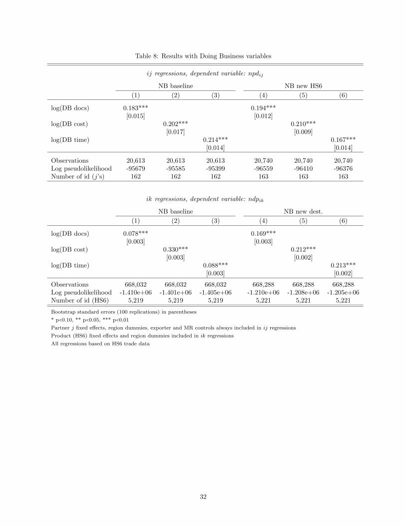
Table 8: Results with Doing Business variables

ij regressions, dependent variable: npdij

NB baseline NB new HS6

(1) (2) (3) (4) (5) (6)

log(DB docs) 0.183*** 0.194***[0.015] [0.012]

log(DB cost) 0.202*** 0.210***[0.017] [0.009]

log(DB time) 0.214*** 0.167***[0.014] [0.014]

Observations 20,613 20,613 20,613 20,740 20,740 20,740Log pseudolikelihood -95679 -95585 -95399 -96559 -96410 -96376Number of id (j’s) 162 162 162 163 163 163

ik regressions, dependent variable: ndpik

NB baseline NB new dest.

(1) (2) (3) (4) (5) (6)

log(DB docs) 0.078*** 0.169***[0.003] [0.003]

log(DB cost) 0.330*** 0.212***[0.003] [0.002]

log(DB time) 0.088*** 0.213***[0.003] [0.002]

Observations 668,032 668,032 668,032 668,288 668,288 668,288Log pseudolikelihood -1.410e+06 -1.401e+06 -1.405e+06 -1.210e+06 -1.208e+06 -1.205e+06Number of id (HS6) 5,219 5,219 5,219 5,221 5,221 5,221

Bootstrap standard errors (100 replications) in parentheses

* p<0.10, ** p<0.05, *** p<0.01

Partner j fixed effects, region dummies, exporter and MR controls always included in ij regressions

Product (HS6) fixed effects and region dummies included in ik regressions


32

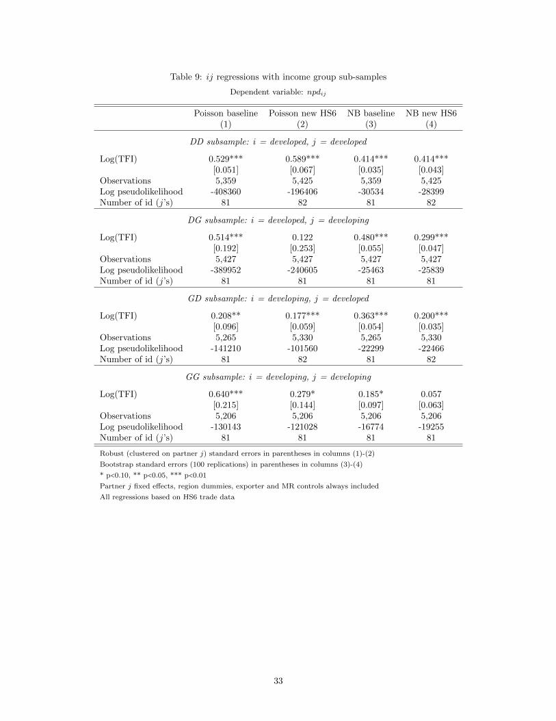
Table 9: ij regressions with income group sub-samples

Dependent variable: npdij

Poisson baseline Poisson new HS6 NB baseline NB new HS6(1) (2) (3) (4)

DD subsample: i = developed, j = developed

Log(TFI) 0.529*** 0.589*** 0.414*** 0.414***[0.051] [0.067] [0.035] [0.043]

Observations 5,359 5,425 5,359 5,425Log pseudolikelihood -408360 -196406 -30534 -28399Number of id (j’s) 81 82 81 82

DG subsample: i = developed, j = developing

Log(TFI) 0.514*** 0.122 0.480*** 0.299***[0.192] [0.253] [0.055] [0.047]


GD subsample: i = developing, j = developed

Log(TFI) 0.208** 0.177*** 0.363*** 0.200***[0.096] [0.059] [0.054] [0.035]


GG subsample: i = developing, j = developing

Log(TFI) 0.640*** 0.279* 0.185* 0.057[0.215] [0.144] [0.097] [0.063]


Robust (clustered on partner j) standard errors in parentheses in columns (1)-(2)

Bootstrap standard errors (100 replications) in parentheses in columns (3)-(4)

* p<0.10, ** p<0.05, *** p<0.01

Partner j fixed effects, region dummies, exporter and MR controls always included


33

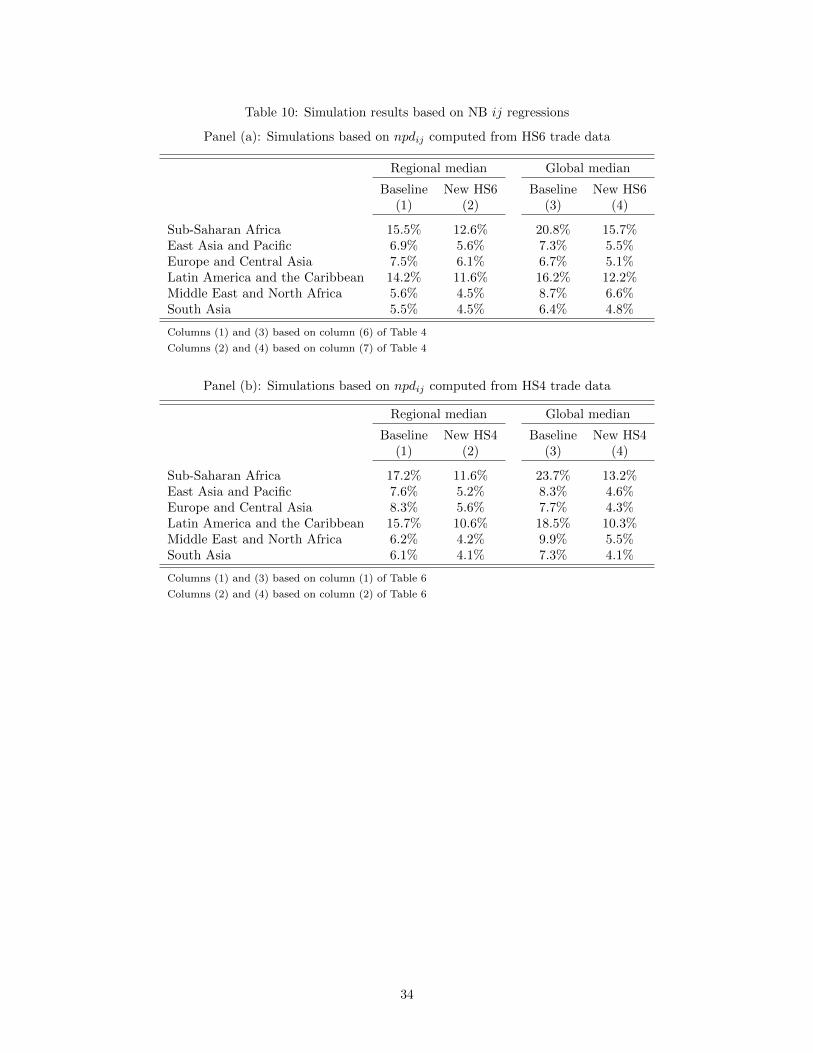
Table 10: Simulation results based on NB ij regressions

Panel (a): Simulations based on npdij computed from HS6 trade data

Regional median Global median

Baseline New HS6 Baseline New HS6(1) (2) (3) (4)

Sub-Saharan Africa 15.5% 12.6% 20.8% 15.7%East Asia and Pacific 6.9% 5.6% 7.3% 5.5%Europe and Central Asia 7.5% 6.1% 6.7% 5.1%Latin America and the Caribbean 14.2% 11.6% 16.2% 12.2%Middle East and North Africa 5.6% 4.5% 8.7% 6.6%South Asia 5.5% 4.5% 6.4% 4.8%

Columns (1) and (3) based on column (6) of Table 4


Panel (b): Simulations based on npdij computed from HS4 trade data


Baseline New HS4 Baseline New HS4(1) (2) (3) (4)




34

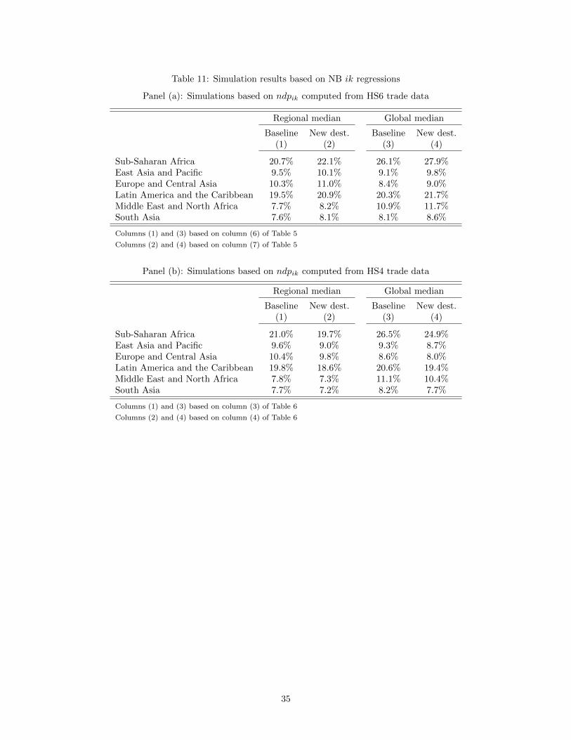
Table 11: Simulation results based on NB ik regressions

Panel (a): Simulations based on ndpik computed from HS6 trade data


Baseline New dest. Baseline New dest.(1) (2) (3) (4)




Panel (b): Simulations based on ndpik computed from HS4 trade data


Baseline New dest. Baseline New dest.(1) (2) (3) (4)




35

Appendix tables

Table A-1: Mapping of OECD TFIs into DCNT and TFA provisions

Indicator DCNT Rev. 18 TFA

A. Information availability Articles 1 and 2 Articles 1 and 2B. Involvement of the trade community Article 2 Article 2C. Advance Rulings Article 3 Article 3D. Appeal Procedures Article 4 Article 4E. Fees and charges Article 6.1 and 6.2 Article 6.1 and 6.2F. Formalities – Documents Articles 7 and 10 Articles 7 and 10G. Formalities – Automation Articles 7 and 10 Articles 7 and 10H. Formalities – Procedures Articles 5, 7 and 10 Articles 5, 7 and 10I. Cooperation – Internal Articles 9.1 and 12 Articles 8.1 and 12J. Cooperation – External Articles 9.2 and 12 Articles 8.2 and 12K. Consularization Article 8 –L. Governance and Impartiality – –M. Transit fees and charges Article 11 Article 11N. Transit formalities Article 11 Article 11O. Transit guarantees Article 11 Article 11P. Transit agreements and cooperation Article 11 Article 11

TFI’s stand for “Trade Facilitation Indicators”

DCNT stands for (WTO’s) “Draft Consolidated Negotiating Text”

TFA stands for (WTO’s) “Trade Facilitation Agreement”

Source: Moıse et al. (2011)

36

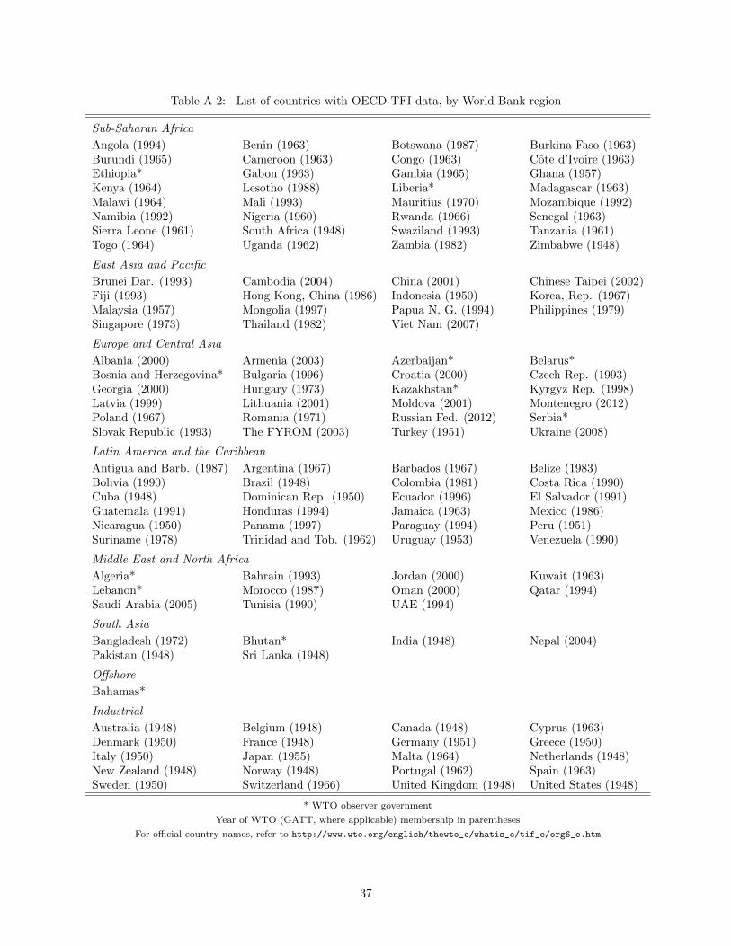
Table A-2: List of countries with OECD TFI data, by World Bank region

Sub-Saharan Africa

Angola (1994) Benin (1963) Botswana (1987) Burkina Faso (1963)Burundi (1965) Cameroon (1963) Congo (1963) Cote d’Ivoire (1963)Ethiopia* Gabon (1963) Gambia (1965) Ghana (1957)Kenya (1964) Lesotho (1988) Liberia* Madagascar (1963)Malawi (1964) Mali (1993) Mauritius (1970) Mozambique (1992)Namibia (1992) Nigeria (1960) Rwanda (1966) Senegal (1963)Sierra Leone (1961) South Africa (1948) Swaziland (1993) Tanzania (1961)Togo (1964) Uganda (1962) Zambia (1982) Zimbabwe (1948)

East Asia and Pacific

Brunei Dar. (1993) Cambodia (2004) China (2001) Chinese Taipei (2002)Fiji (1993) Hong Kong, China (1986) Indonesia (1950) Korea, Rep. (1967)Malaysia (1957) Mongolia (1997) Papua N. G. (1994) Philippines (1979)Singapore (1973) Thailand (1982) Viet Nam (2007)

Europe and Central Asia

Albania (2000) Armenia (2003) Azerbaijan* Belarus*Bosnia and Herzegovina* Bulgaria (1996) Croatia (2000) Czech Rep. (1993)Georgia (2000) Hungary (1973) Kazakhstan* Kyrgyz Rep. (1998)Latvia (1999) Lithuania (2001) Moldova (2001) Montenegro (2012)Poland (1967) Romania (1971) Russian Fed. (2012) Serbia*Slovak Republic (1993) The FYROM (2003) Turkey (1951) Ukraine (2008)

Latin America and the Caribbean

Antigua and Barb. (1987) Argentina (1967) Barbados (1967) Belize (1983)Bolivia (1990) Brazil (1948) Colombia (1981) Costa Rica (1990)Cuba (1948) Dominican Rep. (1950) Ecuador (1996) El Salvador (1991)Guatemala (1991) Honduras (1994) Jamaica (1963) Mexico (1986)Nicaragua (1950) Panama (1997) Paraguay (1994) Peru (1951)Suriname (1978) Trinidad and Tob. (1962) Uruguay (1953) Venezuela (1990)

Middle East and North Africa

Algeria* Bahrain (1993) Jordan (2000) Kuwait (1963)Lebanon* Morocco (1987) Oman (2000) Qatar (1994)Saudi Arabia (2005) Tunisia (1990) UAE (1994)

South Asia

Bangladesh (1972) Bhutan* India (1948) Nepal (2004)Pakistan (1948) Sri Lanka (1948)

Offshore

Bahamas*

Industrial

Australia (1948) Belgium (1948) Canada (1948) Cyprus (1963)Denmark (1950) France (1948) Germany (1951) Greece (1950)Italy (1950) Japan (1955) Malta (1964) Netherlands (1948)New Zealand (1948) Norway (1948) Portugal (1962) Spain (1963)Sweden (1950) Switzerland (1966) United Kingdom (1948) United States (1948)

* WTO observer government

Year of WTO (GATT, where applicable) membership in parentheses

For official country names, refer to http://www.wto.org/english/thewto_e/whatis_e/tif_e/org6_e.htm

37

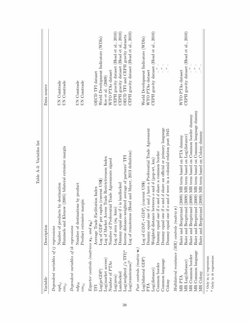
http://www.wto.org/english/thewto_e/whatis_e/tif_e/org6_e.htm

Tab

leA

-3:

Vari

ab

les

list

Var

iab

leD

escr

ipti

onD

ata

sou

rce

Dep

enden

tva

riabl

esofij

regr

essi

on

s

npdij

Nu

mb

erof

pro

du

cts

by

des

tin

ati

on

UN

Com

trad

eem

ijH

um

mel

san

dK

len

ow(2

005)

bilate

ral

exte

nsi

vem

arg

inU

NC

om

trad

e

Dep

enden

tva

riabl

esofik

regr

essi

on

s

ndpik

Nu

mb

erof

des

tin

atio

ns

by

pro

du

ctU

NC

om

trad

eem

ijP

rod

uct

exte

nsi

vem

arg

inU

NC

om

trad

e

Exp

ort

erco

ntr

ols

(matr

ices

x1,

an

dx2)

TF

IA

vera

geT

rad

eF

acil

itati

on

Ind

exO

EC

DT

FI

data

set

Log

(pcG

DP

)L

ogof

GD

Pp

erca

pit

a(c

urr

ent

US$)

Worl

dD

evel

op

men

tIn

dic

ato

rs(W

DIs

)L

og(m

arke

tac

cess

)L

ogof

Mar

ket

Acc

ess

Tra

de

Res

tric

tive

nes

sIn

dex

Kee

etal.

(2009)

Nu

mb

erof

PT

As

Nu

mb

erof

Pre

fere

nti

al

Tra

de

Agre

emen

tssi

gn

edW

TO

PT

As

data

set

Log

(are

a)L

ogof

area

(sq.

km

s)C

EP

IIgra

vit

yd

ata

set

(Hea

det

al.

,2010)

Lan

dlo

cked

Du

mm

yeq

ual

one

ifi

isla

nd

lock

edC

EP

IIgra

vit

yd

ata

set

(Hea

det

al.

,2010)

Log

(wei

ghte

dj’

sT

FI)

aIn

vers

ed

ista

nce

-wei

ghte

dav

erage

of

part

ner

s’T

FI

OE

CD

TF

Ian

dC

EP

IIgra

vit

yd

ata

sets

Log

(rem

oten

ess)

bL

ogof

rem

oten

ess

(Hea

dan

dM

ayer

,2013

defi

nit

ion

)C

EP

IIgra

vit

yd

ata

set

(Hea

det

al.

,2010)

Pair

con

trols

(matr

ixw

)

Log

(bil

ater

alG

DP

)L

ogofGDPi∗GDPj

(cu

rren

tU

S$)

Worl

dD

evel

op

men

tIn

dic

ato

rs(W

DIs

)P

TA

Du

mm

yeq

ual

one

ifi

an

dj

hav

ea

Pre

fere

nti

al

Tra

de

Agre

emen

tW

TO

PT

As

data

set

Log

(dis

tan

ce)

Wei

ghte

dd

ista

nce

bet

wee

no

an

dd

(pop

-wt,

km

)C

EP

IIgra

vit

yd

ata

set

(Hea

det

al.

,2010)

Com

mon

bor

der

Du

mm

yeq

ual

one

ifo

an

dd

share

aco

mm

on

bord

er–

”–

Com

mon

lan

guag

eD

um

my

equ

alon

eifo

an

dd

share

an

offi

cial

or

pri

mary

lan

gu

age

–”

–C

olon

yD

um

my

equ

alon

eifo

an

dd

wer

ein

aco

lon

ial

rela

tion

post

1945

–”

–

Mu

ltil

ate

ral

resi

stan

ce(M

R)

con

trols

(matr

ixr)

MR

PT

AB

aier

and

Ber

gstr

and

(2009)

MR

term

base

don

PT

Ad

um

my

WT

OP

TA

sd

ata

set

MR

Log

(dis

tan

ce)

Bai

eran

dB

ergs

tran

d(2

009)

MR

term

base

don

Log(d

ista

nce

)C

EP

IIgra

vit

yd

ata

set

(Hea

det

al.

,2010)

MR

Com

mon

bor

der

Bai

eran

dB

ergs

tran

d(2

009)

MR

term

base

don

Com

mon

bord

erd

um

my

–”

–M

RC

omm

onla

ngu

age

Bai

eran

dB

ergs

tran

d(2

009)

MR

term

base

don

Com

mon

lan

gu

age

du

mm

y–

”–

MR

Col

ony

Bai

eran

dB

ergs

tran

d(2

009)

MR

term

base

don

Colo

ny

du

mm

y–

”–

aO

nly

inij

regre

ssio

ns

bO

nly

inik

regre

ssio

ns

38

Tab

leA

-4:

Corr

elati

on

s(ij

sam

ple

)

npd

Log(TFI)

Log(pcGDP)

Log(marketaccess)

NumberofPTAs

Log(area)

Landlocked

Log(weightedj’sTFI)

Log(bilateralGDP)

PTA

Log(distance)

Commonborder

Commonlanguage

Colony

np

d1

Log

(TF

I)0.

22*

1L

og(p

cGD

P)

0.35

*0.

39*

1L

og(m

arke

tac

cess

)-0

.00

0.10

*-0

.26*

1N

um

ber

ofP

TA

s0.

23*

0.26

*0.3

3*

0.1

1*

1L

og(a

rea)

0.19

*0.

03*

-0.1

7*

-0.1

0*

-0.0

3*

1L

and

lock

ed-0

.15*

-0.0

5*-0

.32*

0.0

4*

-0.2

1*

0.0

01

Log

(wei

ghte

dj’

sT

FI)

0.19

*0.

23*

0.3

8*

-0.1

0*

0.2

3*

-0.0

6*

0.0

5*

1L

og(b

ilat

eral

GD

P)

0.57

*0.

29*

0.4

0*

-0.1

0*

0.2

4*

0.3

2*

-0.2

1*

0.1

4*

1P

TA

0.25

*0.

09*

0.0

9*

0.0

4*

0.3

2*

-0.0

0-0

.08*

0.0

6*

0.1

7*

1L

og(d

ista

nce

)-0

.29*

-0.0

2*-0

.053

0.0

7*

-0.1

4*

0.0

6*

-0.0

5*

-0.1

1*

-0.0

7*

-0.4

0*

1C

omm

onb

ord

er0.

23*

0.01

-0.0

1-0

.01

0.0

10.0

5*

0.0

2*

0.0

10.0

5*

0.2

1*

-0.3

7*

1C

omm

onla

ngu

age

0.05

*-0

.06*

-0.0

8*

0.1

0*

-0.0

4*

-0.0

4*

-0.0

1-0

.18*

-0.1

3*

0.1

1*

-0.1

1*

0.1

2*

1C

olon

y0.

12*

0.02

*0.0

5*

0.0

00.0

5*

0.0

2*

-0.0

2*

0.0

3*

0.0

8*

0.0

3*

-0.0

3*

0.0

5*

0.1

4*

1

Corr

elati

on

sco

mp

ute

dfr

om

the

sam

ple

of

colu

mn

(6)

of

Tab

le4

*p<0.0

5

39

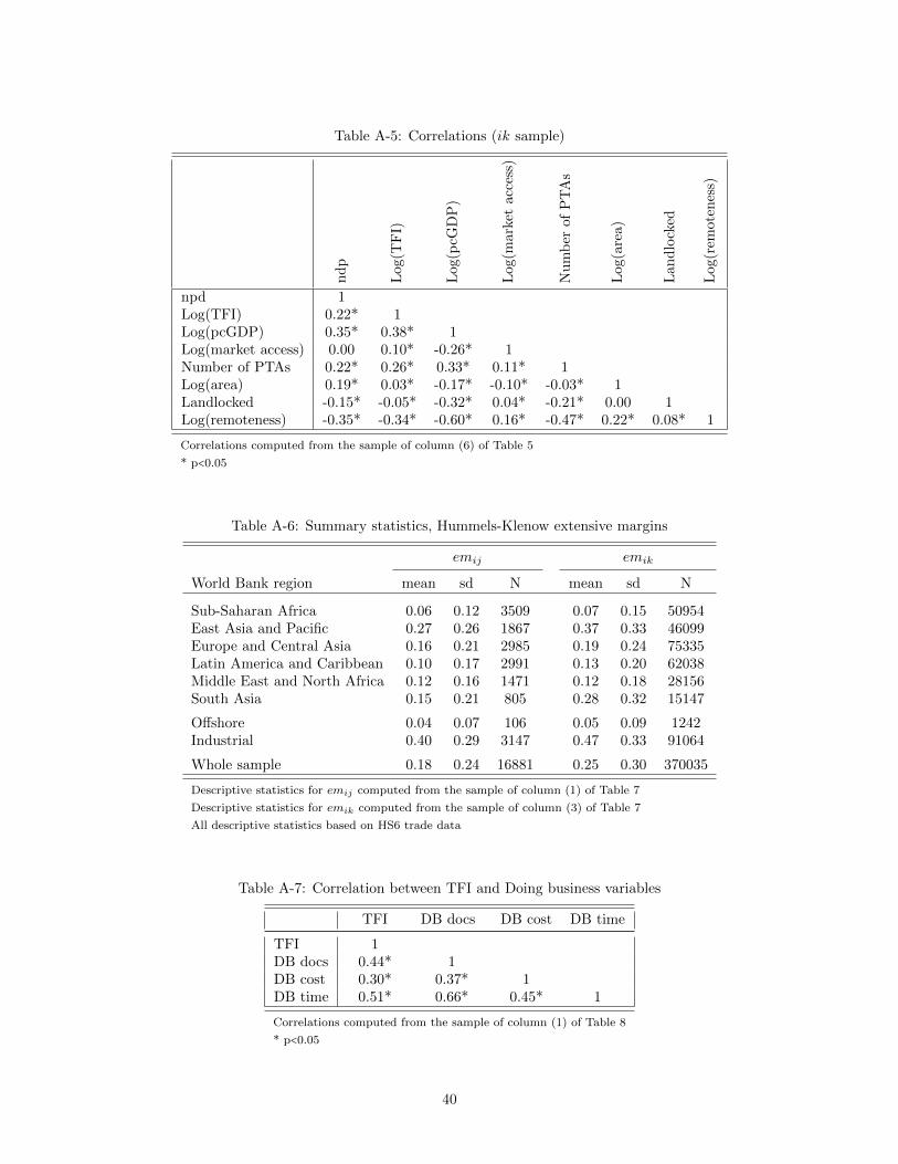
Table A-5: Correlations (ik sample)

nd

p

Log(

TF

I)

Log(

pcG

DP

)

Log(

mar

ket

acc

ess)

Nu

mb

erof

PT

As

Log(

are

a)

Lan

dlo

cked

Log(

rem

ote

nes

s)

npd 1Log(TFI) 0.22* 1Log(pcGDP) 0.35* 0.38* 1Log(market access) 0.00 0.10* -0.26* 1Number of PTAs 0.22* 0.26* 0.33* 0.11* 1Log(area) 0.19* 0.03* -0.17* -0.10* -0.03* 1Landlocked -0.15* -0.05* -0.32* 0.04* -0.21* 0.00 1Log(remoteness) -0.35* -0.34* -0.60* 0.16* -0.47* 0.22* 0.08* 1

Correlations computed from the sample of column (6) of Table 5

* p<0.05

Table A-6: Summary statistics, Hummels-Klenow extensive margins

emij emik

World Bank region mean sd N mean sd N

Sub-Saharan Africa 0.06 0.12 3509 0.07 0.15 50954East Asia and Pacific 0.27 0.26 1867 0.37 0.33 46099Europe and Central Asia 0.16 0.21 2985 0.19 0.24 75335Latin America and Caribbean 0.10 0.17 2991 0.13 0.20 62038Middle East and North Africa 0.12 0.16 1471 0.12 0.18 28156South Asia 0.15 0.21 805 0.28 0.32 15147

Offshore 0.04 0.07 106 0.05 0.09 1242Industrial 0.40 0.29 3147 0.47 0.33 91064

Whole sample 0.18 0.24 16881 0.25 0.30 370035

Descriptive statistics for emij computed from the sample of column (1) of Table 7

Descriptive statistics for emik computed from the sample of column (3) of Table 7

All descriptive statistics based on HS6 trade data

Table A-7: Correlation between TFI and Doing business variables

xxTFIxx DB docsx DB cost DB time

TFI 1DB docs 0.44* 1DB cost 0.30* 0.37* 1DB time 0.51* 0.66* 0.45* 1

Correlations computed from the sample of column (1) of Table 8

* p<0.05

40