Export Composition and Growth.

Fergal McCann

School of Economics

University College Dublin

August 2007

Export Composition and Growth

TABLE OF CONTENTS Acknowledgements i Preface ii 1: Introduction 1 2: Literature Review 5 3: Empirics 18

3.1: EXPY Calculation 18

3.2: Data and Methodology 20 3.3: Results 23

4: Growth Regressions 29

4.1: Data and Methodology 29

4.2: Regressions and Results 29

5: A look at the Irish story 32 6: Conclusion 43 Bibliography 46 Appendix: Tables 50

Export Composition and Growth

Index of Tables Table 1: Sample Size by Year Table 2: PRODY Results by Year and Sector Table 3: Global EXPY Average by Year Table 4a-4f: Selected EXPY Results by Year, 1980-2003 Table 5: Countries Included in Panel Growth Regression 1 Table 6a: High-Income Countries Included in Panel Growth

Regression 2

Table 6b: Low-Income Countries Included in Panel Growth Regression 3 Table 7: Panel Regression Results

Export Composition and Growth

ABSTRACT The relationship between exports and growth has been formalized in the Export-Led-Growth (ELG) hypothesis. A huge literature has grown around the testing of this hypothesis, with mixed results and scepticism regarding direction of causality. The importance of the composition, rather than the volume of a country’s export basket has been given less attention in the literature. This study, using the technique applied by Rodrik, Hausman and Hwang (2006), aims to present the importance of export composition in economic growth. Using World Development Indicators data across ten export sectors for a sample of countries ranging from 77 to 117, an index PRODY is calculated to measure the “sophistication” level of each export sector. The underlying thought for this calculation is the Heckscher-Ohlin view of the global economy, whereby richer countries should export more technologically sophisticated goods. An EXPY index of the sophistication of each country’s export basket is calculated from the weighted sum of PRODY values, with weight given to the share of each sector in each country’s exports. EXPY is included in a balanced panel growth regression and evidence of a causal effect from EXPY to growth is found. When the panel is divided into upper and lower income countries, the effect is accentuated for lower-income countries, giving rise to interesting policy implications for economic development.

i

Introduction

1 INTRODUCTION

The idea that trade can be the engine of economic growth goes back as far as

Adam Smith, and his theories on specialization. Despite this long historical

theoretical link, throughout the twentieth century many writers offered their

views on why trade was bad for development. Authors such as Prebisch and

Singer developed theories such as the “Import Substitution Industrialization”

theory. This was based on the view that a secular decline in raw materials

prices would cause the gap between developed and developing countries to

worsen due to the fact that developing countries usually exported heavily in

raw materials. Therefore, poorer countries would need to industrialize to

develop, and to do this would need protection in the form of trade barriers in

order to nurture indigenous infant industry. Marxist writers went further and

said that poor countries should not trade at all with the so-called “north”.

Despite these anti-trade theories, there exists a vast literature on the links

between trade and economic growth and development. A lot of the literature

consists of analysis and testing of the Export-Led Growth (ELG) hypothesis.

This hypothesis states that promotion of the export sector is the best way to

achieve economic growth. This is a valid hypothesis and there are many

explanations as to why exports are a crucial way to obtain growth. The

demand-side argument is that domestic markets severely limit the scope for

sales of a domestically produced product, and that exports open domestic

industries up to foreign markets, hugely increasing the potential demand for

the product. This increase in potential market size can lead to increasing

returns, whereas the home market may have been too small to achieve

optimal scale. The economies of scale that can be achieved from exporting

lead to increased capacity utilization, which results in greater product variety

and productivity gains. Greater exposure to world markets may induce

competitive pressures and may spur innovation and facilitate technological

advancement and knowledge spillovers into the domestic economy, that lead

to technological upgrading and efficiency gains in production and

management practices. Evidence of this effect, which will be cited quite

1

Introduction

1regularly, comes in Gorg and Strobl (2005). Exports also generate much-

needed foreign exchange, which can be used to provide the public funds

needed to divert production towards the most growth-enhancing industries.

This specialization towards more productive export industries and away from

relatively inefficient sectors increases human capital through an increase in

the general skill level of the country. Another argument for the ELG

hypothesis is that it may be seen as part of the product and industry lifecycle

hypothesis. This hypothesis describes economic growth as a cycle that begins

with exports of primary goods. Over time, economic growth and knowledge

change the structure of the domestic economy, including consumer demand,

which propels the more technology-intensive domestic industry to begin

exporting. As domestic demand ebbs, economic growth arises from

technologically advanced exports.

The author’s view, which sets the context for the rest of this paper, is

that trade is not an end in itself. It is not simply the case that a country can

simply increase its exports per se and be sure of experiencing economic

growth, but rather it is the composition and the concentration of these exports

that counts.

The structure of a country’s export basket is the important factor in

encouraging economic growth through exports. How the structure of a

country’s export basket comes about can be viewed through the lens of

Heckscher-Ohlin trade theory. This theory assumes identical production

technology everywhere and assumes that the only difference between

countries is in their relative abundances of capital and labour. The varying

factor proportions between countries determine a country’s basket of goods

produced. Countries that produce technologically more intensive goods are

those with a relatively high capital-labour ratio. Another possibility is that the

level of human capital in such countries is high, which is evidenced by a high

skilled-to-unskilled labour ratio. Such countries are usually developed

countries. Poorer countries usually have a lower capital-labour ratio, a low

skilled-to-unskilled labour ratio and thus, produce goods that are more labour

intensive and less technologically sophisticated. In general, one can posit that

2

Introduction

countries tend to export goods whose production makes intensive use of

resources of which they have a relatively large supply and, conversely, to

import goods which require large inputs of resources that are locally scarce.

Later exponents of Heckscher-Ohlin theory, e.g. Mayer & Wood (2001) regard

the following three resources as those whose variation affects export

composition: skill (human capital acquired through education or training), land

(meaning natural resources of all sorts) and labour. Capital is omitted as it has

become an almost completely freely tradable commodity and, therefore,

cannot be regarded as giving a country a relative comparative advantage from

being part of its resource endowment. If a country has a comparative

advantage in a resource such as zinc or copper or labour, it can easily obtain

the capital needed to develop this resource and to set up an export industry

around this resource. While this is a very simplistic model with many strong

assumptions, the basic findings of it are very relevant to any analysis of export

composition across countries. While this paper will not look in detail at the

explanation behind countries’ export compositions, this Heckscher-Ohlin

analysis will provide a good background that can be referred to when looking

at the results presented in Section 3.

Section 2 will provide a review of the literature on the ELG hypothesis,

and, more specifically on the link between export composition and growth.

Section 3 will take from the work of Hausmann, Hwang and Rodrik (2005),

who calculate an index, which they call EXPY, which is a measure of the

sophistication of a country’s export basket. It is this index that forms the main

empirical section of this paper. Further detail on the intuition behind this index

and its calculation will be provided in Section 3. Section 3 will also provide the

sources and explanation of all data used. In Section 4, standard growth

regressions will be presented, with the inclusion of EXPY for each country as

an independent variable. A more formal analysis of the effect of export

composition on growth will be possible from these regressions. Conclusions

will be drawn from the study in Section 5.

3

Literature Review

2 LITERATURE REVIEW A brief overview of the Export-Led Growth (ELG) literature will be carried out,

before moving on to the literature on export composition. There are many

plausible reasons within trade theory to support the ELG hypothesis. Broadly,

the focus of the ELG debate is on whether a country is better served by

orienting trade policies towards export promotion or import substitution.

Examples such as the economic success of the outward-oriented Asian “tiger”

economies would seem to suggest the ELG hypothesis is valid. The

effectiveness of export promotion as an engine for economic growth is, in the

end, an empirical issue.

Most authors who look at the ELG hypothesis will cite the same logical

reasons for supporting the ELG in their introductions. Where they differ

however, is in their methods of testing the hypothesis. They vary in the

econometric techniques used, in the samples of countries used, and in the

indicator for exports used.

Early work examining the ELG hypothesis includes that of Michaely

(1977) and Balassa (1978). These papers use the rank correlation technique

with Michaely using averaged GNP per capita growth and averaged growth in

export share, and Balassa using average growth in real GNP and growth in

real exports. Both authors find a statistically significant positive export-

economic growth relationship. Michaely’s findings must be qualified further

however, as he finds that a minimum threshold of development is needed

before the association can exist. This is a plausible hypothesis that appears

quite regularly in the literature – that the poorest countries cannot use exports

as an engine for growth; they must first reach a certain ‘threshold’ level of

development before this is possible. Balassa also carries out an OLS growth

regression with averaged GNP growth as the independent variable, and

averaged growth in real exports, averaged labour force growth, averaged

domestic investment as a share of output and averaged foreign investment as

a share of output as the dependant variables. From this growth regression, he

also finds a positive export-economic growth relationship, although the results

from a simple OLS regression must be viewed with caution, as they do not

take the possible endogeneity of exports into account. Giles and Williams

4

Literature Review

(2000) claim that the positive association that these types of cross-country

studies find “is as compatible with GLE as with ELG or feedback effects”,

where GLE refers to Growth-Led Exports and the issue of reverse causality.

Other studies to carry out variants of OLS growth regressions include

Balassa (1981), Jaffee (1985), Kohli and Singh (1989), Fosu (1990) and Park

and Prime (1997). All of these studies use some combination of investment,

education or human capital, population growth and labour force growth, along

with export growth or export share of GDP, as their dependent variables. All

find a positive relationship between exports and economic growth. Once

more, any OLS cross-country results must be viewed skeptically.

The work of Feder (1983) is seen as something of a seminal

contribution to the export literature. According to Ibrahim and MacPhee

(2003), this study was “the first attempt to model an explicit link between trade

and growth”. In the study, Feder hypothesizes that there is one mechanism

causing the link between trade and growth, namely the higher productivity of

the export sector relative to the domestic non-export sector. Feder puts

forward a number of reasons as to why this productivity differential can lead to

increased growth across the whole economy. Examples of reasons for the

export sector becoming more productive include the need for domestic

management practices to become more efficient in the face of stiff foreign

competition; increased awareness of technical progress abroad creating

incentives for innovation at home; firms taking advantage of economies of

scale due to the ability to increase production in the face of the increased

demand from new markets. Feder tested his proposition using a dataset of 31

developing countries for the years 1964-73. He found the productivity

differential to be significant for all countries.

With reference to the impact of the export sector on the rest of the

economy, Feder (1983) proposed the following reasons for an externality

effect from the export to the domestic sector: the training of higher quality

labour; a steady flow of imported inputs; introduction of new production

techniques. Feder tested this hypothesis and found a positive and statistically

significant externality coefficient.

Ibrahim and MacPhee (2003) themselves use Feder's model but apply

new data for 30 developing countries from the years 1974 to 1993. Feder's

5

Literature Review

extremely strong support for the ELG is not supported by their econometric

analysis. They found that for 18 of the 30 countries analyzed, there is a

positive and statistically significant productivity differential for the export sector

relative to the domestic sector and that 13 countries have positive and

significant externality coefficients. Support for Feder's hypothesis is still found,

but it is not as strong. Interestingly from the viewpoint of this study the authors

find that the export-non-export differential seems to be strongest in those

countries that export manufactured products rather than primary goods. They

also find that “strong – or moderate – outward orientation, a well-diversified

export structure and highly processed export products generally characterize

countries with export sectors that generate positive externalities for the non-

export sector”.

Unlike the cross-country literature, there is much less consensus on

the ELG hypothesis in the time-series literature. There is a much higher

proportion of authors who reject the ELG hypothesis than in the cross-country

literature. Giles and Williams (2000), in their survey of the empirical literature

on the ELG, point out that 74 per cent of the time series literature reviewed

used some form of Granger’s causality test, with the other 26 per cent using

time series data to estimate regression models that do not incorporate

dynamic effects. Emphasis is put on the ‘atheoretical’ nature of Granger’s test,

in that no a priori restrictions are put on the relationships between the

variables of interest.

Examples of time-series studies that find support for the ELG

hypothesis include Abou-Stait (2005) for Egypt, Awokuse (2002) Canada. In

contrast to these two studies, Henriques and Sadorsky (1996) find that

economic growth in fact precedes exports, i.e., support for the GLE (Growth-

Led Exports) hypothesis. Others find bi-directional causality, and some, such

as Darrat (1986), Grabowski et al. (1990) and Serletis (1992) find no causality

at all for some of the countries or time periods of their study.

Herzer, Nowak-Lehmann and Siliverstovs (2004) examine the ELG

hypothesis for Chile using annual time series data in a production function

framework. It differs from other time series work in that it disaggregates total

exports into primary and manufactured exports, looking at their effect on

productivity growth, rather than simply on the effect of aggregate exports.

6

Literature Review

Primary product exports were found to have a statistically significant negative

impact, whereas manufacturing exports were found to have a statistically

significant positive impact on non-export GDP. These results were shown to

be robust to different estimation techniques. The authors claim, “in connection

with the theoretical foundations underpinning our model, the estimation results

can be interpreted as evidence of productivity-enhancing effects of

manufactured exports and of productivity-limiting effects of primary exports”.

They identify one of the main issues put forward in the introduction to this

paper when trying to explain the link between export composition and growth:

“manufactured exports might offer greater potential for knowledge spillovers

and other externalities than primary exports”.

Crespo-Cuaresma and Wörz (2005) group manufacturing industries

into two broad groups, referred to as low and high-technology activities, based

on the classification by Hatzichronoglou (1997). This is a classification based

on R&D intensity in a specific industry taking into account purchases of

intermediaries and capital goods from other sectors. In their model GDP

growth is regressed on share of investment in GDP, population growth, non-

manufacturing exports, low-technology exports and high technology or

technology-intensive exports. High-tech exports are found to have a

significant positive effect, with low technology manufacturing now exhibiting a

significant negative effect.

One final interesting result from this study arises when the sample of

countries is divided into OECD and non-OECD countries. For the group of

industrialized countries, there is no significant effect of the productivity

differential of the export sector relative to the domestic sector on economic

growth. This significant positive effect exists only for developing countries.

This would concur with the view of Balassa (1981): ‘for given increments of

capital, labour and exports, the rate of economic growth will be higher the

lower is the level of development’. Thus, the authors conclude that developing

countries can experience gains from opening up to international trade via

“improved resource allocation as a result of their exposure to international

competition”, while learning effects and other positive externalities are found

to not be of much importance.

7

Literature Review

In Greenaway et al. (1999) exports are disaggregated further in this

study into fuel, food, metals, other primary, machinery, textiles, and other

manufactures, making it the most similar in terms of aggregation to this paper.

They introduce exports into a traditional growth theory framework, with GDP

per capita being explained by initial GDP (to pick up ‘catch up’ effects), level

of secondary school enrollment, a terms of trade index, population, share of

investment in GDP and, in the first regression, an export ratio variable, and

secondly, share of each export sector in GDP. The first regression carried out

is, thus, effectively a test of the ELG hypothesis. Even after controlling for

endogeneity of the export variable and correcting the dependent variable for

growth accounting effects, the export variable still has a positive and

statistically significant effect on economic growth. Once exports are divided

into the above-mentioned categories, fuels, metals and textiles appear to be

the most important drivers of economic growth. The authors point out that this

should be expected, due to the relative importance of the textile sector to

developing countries and due to metals and fuels being inputs in industrialized

countries.

Schott (2006) provides a useful theoretical explanation for export

composition. Embedded within the Hecksher-Ohlin framework, he is able to

explain China’s export composition, which is more sophisticated than would

be expected, which is also found in the empirical section of this paper. The

reason proffered relates to factor distribution “lumpiness”. As a whole, China

should specialise in labour-intensive goods due to its factor endowment.

However, the reality is there are certain areas within the country that are in

fact skill-abundant, thus having a comparative advantage in skill-intensive

products. Thus China’s export composition is not as labour-intensive as one

would expect at first glance. This phenomenon is to be expected in larger

countries, which by definition should have a higher level of factor variation

within their borders. It is certainly a possible explanation for some results in

this paper.

The studies that have most influenced this paper are Hausmann, Hwang and

Rodrik (2005); 'What you export matters', and Rodrik (2006); 'What's so

special about China's exports?' These studies are the first to make use of the

PRODY and EXPY indices as methods of calculating measures of export

8

Literature Review

sophistication. Details on the intuition behind these indices and their

calculation are included in Section 3. The authors argue, citing Hausmann

and Rodrik (2003); 'Economic development as self-discovery', that it is not

only the normal fundamentals such as endowments and institutional quality

that determine a country's specialization pattern, but also the number of

entrepreneurs in a country that embark on ventures which, if successful, will

lead to huge positive externalities for other potential investors in that

economy. It is this characteristic which the authors refer to as the

“idiosyncratic” element in the determination of a country’s export composition,

i.e., that which cannot be explained by normal fundamentals. They argue that

such entrepreneurs are effectively testing the cost structure of the economy

for all other potential investors, carrying huge personal risk as they delve into

the “unknown”. While if they succeed, the emulation of their venture by other

investors in effect “socializes” the externality, if they do not succeed, the

losses remain private. This leads to a sub-optimal amount of the knowledge

externality in the economy unless the government can find a way to

internalize the externality. An example of such a mechanism being put in

place is the Korean government's subsidizing and offering of cheap bank

credit to many firms, particularly in the electronics industry. This was done

with the aim of overcoming the sub-optimal provision of the positive externality

associated with enterprising projects. Where the Korean government differed

from other state-sponsored schemes was through their controlling of the

available credit through state-owned commercial banks. They were very quick

to pull support for enterprises if available information suggested that

productivity would lag. They could freeze bank credit on any poorly performing

ventures that they had aided. Through this scheme, only truly exceptional

performers made it through, the result being the spectacular performance of

the Korean economy as the century wore on, with the electronics industry

serving as an engine for economic growth. As an example of the

government's ruthlessness, only three of the top ten performing government-

aided enterprises in 1965 made it onto the same list in 1975, with only seven

from the 1975 list making it onto the 1985 list. Taiwan's similar economic

success has its roots in an identical strategy aimed at the textiles industry,

which started in the 1950's, as did Japan with its computer industry.

9

Literature Review

The link between this hypothesis and the calculation of PRODY and

EXPY indices can be summarized by quoting Hausmann, Hwang and Rodrik

(2005): “some traded goods are associated with higher productivity levels

than others and … countries that latch on to higher productivity goods

(through the cost discovery process just described) will perform better”. It is

through this thought process and with this logic that the authors justify the

calculation of PRODY and EXPY. These indices aim to identify products that

have high sophistication levels and, therefore, growth-enhancing effects.

Once identified, it is postulated that countries that can position themselves

such that their export basket is comprised mainly of goods with high levels of

PRODY (thus ensuring a high EXPY level as EXPY is the weighted sum of

the PRODY values of goods exported) are the countries with the greatest

potential for growth and development. The authors find some interesting

results. Two of the most important results are those for China and India.

These are two countries that have experienced great growth in recent years.

The results from this study show both countries, and in particular China, to

have EXPY levels far greater than would have been expected given their

income levels. It is this revelation that inspired Rodrik (2006) to investigate

further in the study ‘What’s so special about China’s exports?’ China and

India’s relatively high EXPY ratings imply that these countries are exporting a

range of goods that is far more sophisticated than one would have thought. As

was demonstrated in the work of Schott (2006), China does not fit into the

multiple-cone equilibrium of the Heckscher-Ohlin framework, which suggests

that it would produce only low-skilled labour-intensive goods, in line with its

factor endowments. The fact that this is not the case for China can be

explained by Schott’s idea of lumpiness of the distribution of factors within the

country, with some areas high in physical and human capital accounting for

the surprisingly sophisticated export structure, perhaps more so than by the

self-discovery idea of Hausmann and Rodrik (2003). The Indian case has

proven even harder to explain. It is the Information Technology (IT) sector that

has been the motor for India's high economic growth, yet India is certainly not

a country that would be expected to have a comparative advantage in IT. It

has low levels of IT penetration indicators, has not latched on to any other

high-tech sectors, and is relatively highly endowed in low-skilled workers. One

10

Literature Review

reason given is the fact that work sent from the US at close of business that is

being processed in cities such as Bangalore is ready at the start of business

in the US due to the time difference, making this outsourcing a very efficient

option. The proficiency of many Indians in the English language, along with

the impressive structure of Indian Institutes of Technology, are also

mentioned.

In summarizing the work of Hausmann et al. (2005), the clear

implication is, like in many of the studies cited above, that gains from trade

occurring due to globalization are not unlimited and unqualified. For a country

to gain from trade, it must be able to latch onto certain industries that are

placed highly along the quality spectrum, proxied in this study by the PRODY

index.

11

Empirics

3 EMPIRICS 3.1 EXPY Calculation It would be constructive at this point to introduce Balassa’s (1965) concept of

Revealed Comparative Advantage (RCA). RCA for country i and industry j is

defined as

ii

ij

iijij XX

XXRCA

//

1∑=

=

If we take the example of Ireland’s RCA for Insurance and Financial services,

the figure calculated is the share of Ireland’s export share in this industry

relative to the share of motor vehicles in total world exports. From this

calculation, we can say that if RCA Ireland, Insurance and Financial Services >1, then

Ireland has a Revealed Comparative Advantage in this sector. This is the

essence of the Balassa measure. RCA is used as a weight for every country

exporting in a sector below in the calculation of PRODY, which is the proxy

measure used here of a product or sector’s Total Factor Productivity.

EXPY is a measure of the sophistication of a country’s export basket. In order

to calculate EXPY for each country, PRODY must first be calculated, which is

a weighted average of the incomes of the countries exporting a good.

Because higher-income countries tend to be more capital-abundant, and thus

through the lens of the Heckscher-Ohlin framework should produce more skill

or capital-intensive goods, this RCA-weighted average of incomes is a valid

proxy for the productivity or sophistication of a particular export good. Let

countries be indexed by j and sectors be indexed by k. Total exports of

country j are thus given by

∑=k

jkj xX

By denoting the per-capita GDP of country j as Yj, the following expression for

PRODYk is arrived at:

jj j jjk

jjkk Y

XxXx

PRODY ∑∑≡

)(

12

Empirics

What this means is that PRODY is an RCA-weighted average of the incomes

of countries exporting that good, where the weights correspond to the RCA of

each country in good k. The mapping of an RCA-weighted index to

productivity has the potential to cause controversy. Yi (2003) points to the

work of Davis (1995) to allay such fears. Davis presents a model in which

interindustry trade is determined by Heckscher-Ohlin forces, while

intraindustry trade is determined by Ricardian forces. Davis’ theoretical

framework confirms a positive relationship between the relative productivity of

an industry and its RCA. Yi also calculates correlation between manufacturing

relative TFP measures drawn from Harrigan (1997a, 1997b, 1999) and RCAs

computed from OECD input-output tables for 1985. The correlation found is

.31, which is taken to be sufficient to demonstrate a link between the two. This

gives us the theoretical and empirical backing to continue with PRODY being

used as a proxy for Total Factor Productivity in an industry. To quote form Yi:

As the number of goods for which a country has higher relative productivity

increases, exports from that industry will increase, as will the country’s RCA.

This quantitative index also allows the idea of Hausmann et al. (2005)

regarding the “idiosyncratic” element of the determination of a country’s export

basket to be factored in, whereby certain countries will have export baskets

that are more sophisticated than would have been expected in a H-O world,

given their endowment. Some examples of this appear in the results section,

where countries appear towards the top of global EXPY standings despite

having a per-capita GDP that would lead us to predict a much lower EXPY

value.

Focus can now be turned to the calculation of the EXPY index for each

country j. EXPYj is defined as the sophistication level associated with a

country’s export basket. It is calculated simply as the weighted sum of the

PRODY values for each sector k where the weights are the value share of

sector k in country j’s export basket.

kk j

jkj PRODY

Xx

EXPY ∑=

This gives the weighted averages of the GDP per capita of all countries

exporting the same goods as country j, where the weights are as described

13

Empirics

above. This can then be interpreted as the quality or sophistication level of

country j’s export basket. Some aforementioned reasons can be cited to

explain the importance of a high EXPY value. These include the greater

potential for knowledge and technology spillovers into the domestic sector

from skill and capital intensive activities, the exposure to more efficient foreign

management practices and the incentive for innovation brought about by

exposure to foreign competition.

To put the values that countries attain given the data in this paper in

context, it is possible to put lower and upper bounds on EXPY. 2003 values

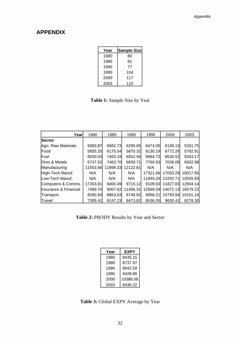
are arbitrarily cited for demonstration purposes (see Table 2). The lower

bound would be attained if a country had 100% of its exports in the sector with

the lowest PRODY rating. In this paper that would imply an EXPY of

$5,331million, in 2003, which would be attained if a country had 100% of its

exports in the Agricultural Raw Materials sector. The upper bound, on the

other hand, would be attained if a country had 100% of its exports in the

sector with the highest PRODY score. In this paper, for 2003, this would imply

an EXPY value of $16,579million, which would be attained if a country had

100% of its exports in the Insurance and Financial Services sector.

In this, the first empirical section of this paper, EXPY values for samples of

countries for the years 1980, 1985, 1990, 1995, 2000 and 2003 will be

calculated. In doing this the sectors with the highest PRODY values will be

identified. The countries that have the highest EXPY values and how these

values have evolved over time will also be identified, thus giving an idea of

which countries have derived the greatest advantage from their export basket.

The calculation of PRODY and EXPY values attempts to identify the most

growth-enhancing sectors and to show which countries are employing the

“best” export strategies.

3.2 Data and Methodology GDP per capita data are from the World Development Indicators (WDI) for

2005, obtained from the World Bank. The series used is GDP per capita, PPP

(constant 2000 international $). By using such a measure for GDP, correction

is made both for differences across time (inflation) and differences across

14

Empirics

countries (deviations from purchasing power parity). This means that all

PRODY and EXPY calculated using this measure of income will be fully

comparable across all time periods and countries.

All export data have also been taken from the WDI. The years examined

are 1980, 1985, 1990, 1995, 2000 and 2003. The data are given in millions of

current US Dollars. For the years 1980, 1985 and 1990, total exports are

broken down by country into 9 sectors, which come in two categories. The

first category is referred to as ”Merchandise Exports”. This category contains

the following sectors:

• Agricultural Raw Materials

• Food

• Ores and Metals

• Fuels

• Manufacturing

The second category is referred to as “Commercial Service Exports”, and

contains the following sectors:

• Transport Services

• Travel Services

• Insurance and Financial Services

• Computer and Communications Services

The only difference between this breakdown and that for the years 1995,

2000 and 2003 is that the sector entitled “Manufacturing” no longer exists and

is instead broken down and replaced by the sectors entitled “High-Tech

Manufacturing” and “Low-Tech Manufacturing”. This leads to a total of 10

sectors for the final three years examined. A limitation of this data is that the

level of aggregation does not allow for heterogeneity within sectors to be

accounted for. For example, within a sector such as Manufacturing, there are

products with hugely varying sophistication levels, yet a PRODY value is

given for the sector as a whole. This means that countries that could in fact be

exporting quite different products within a given sector are being attributed the

same value for that sector in the calculation of their EXPY value. Despite this,

15

Empirics

the data does still allow a good opportunity for global trends in trade to be

observed over the sample period.

The size of the sample of countries for which EXPY could be calculated

is reported in Table 1. It ranges from a maximum of 117 in 2000 to a minimum

of 77 in 1990. One reason for this inconsistency is that a number of the

countries reporting in the latter years of the survey did not exist until the early

1990’s. They include the former Yugoslav states such as Croatia, Slovenia

etc., and former Soviet states such as Armenia, Estonia, Latvia, Lithuania,

Belarus, Ukraine, etc., as well as the Czech Republic and Slovakia. Aside

from the fact that these countries are missing, however, one must be very

wary of smaller sample sizes, as the non-reporting of data is generally found

to be highly negatively correlated with income.

The data that were used in calculating PRODY and EXPY for each

year will now be specified. Separate PRODY scores are calculated for each of

the years in the sample, applying the WDI export data to the formula specified

in Section 3.1. The PRODY score for each separate year is used in

calculating each country’s EXPY value for that particular year. An alternative

approach is used by Hausmann et al. (2005). They calculate PRODY values

for each year, but then take an average figure from the three years that had

the highest number of countries reporting. It is this average PRODY value that

is used to calculate EXPY in each year. This method is disadvantageous as it

fails to take account of changes in global trade patterns over the period.

Rather, it simply tracks how the composition has changed within countries,

with no regard for the fact that the sophistication of sectors, as measured by

the RCA-weighted sum of the countries exporting them, may also change

over time. The downside to using PRODY for each year is that there should

be a tendency for EXPY to grow over time, seeing as PRODY should grow

with GDP growth. Despite this expectation, we still see PRODY figures drop

across certain time periods, meaning that EXPY figures can indeed decrease

over time if export baskets are oriented towards the wrong sectors. It is not

lost on the author however that this property does render the ordinal ranking

of EXPY more important than the cardinal. It is still felt that this is a worthwhile

approach in that the global trends in trade are not glossed over by using an

average PRODY figure.

16

Empirics

In the results section, it is clear that over the different years of the

sample, the importance of some sectors, notably the Insurance and Financial

Services sector, has increased relentlessly, while other sectors have

remained stagnant and have even decreased in their sophistication levels,

proxied by the weighted average of the incomes of the countries exporting

them. The issue of non-comparability of data does not arise, as the data used

are PPP-adjusted, constant 2000 international $, meaning that even if

PRODY is calculated for different years using different income levels, they are

still fully comparable.

An advantage of the methodology used to calculate PRODY is

explained using an example. The rationale behind using comparative

advantage as a weight is so that country size does not distort the rankings. If

weighted averages were not used, the raw figures for the exports of the

world’s richest countries would render the data for poorer countries negligible.

As an example, the exports of Agricultural Raw Materials for Benin and Brazil

will be examined. In 2000, Benin’s exports in this sector amounted to

$281.82million, whereas Brazil’s amounted to $2.62billion. This figure for

Benin accounted for 54.37% of their exports in 2000, whereas the figure for

Brazil accounted for a mere 4.15%. This means that in the weighted method

of calculating PRODY for Agricultural Raw Materials, Benin’s income will have

a larger weighting than Brazil’s income, even though Brazil’s absolute volume

of Agricultural Raw Materials exports is far larger than Benin’s. This property

means that the results expected by the underlying Heckscher-Ohlin

framework are more likely to occur. Low-income countries with heavy

dependence on low-sophistication sectors will account for relatively larger

amounts of the PRODY figure for these sectors, with rich countries’ incomes,

due to their small export share in these sectors such as Agricultural Raw

Materials, not giving much weight to that sector’s PRODY. Conversely, rich

counties with relatively large export shares in more sophisticated sectors will

drive high PRODY values for these sectors.

3.3 Results PRODY results for each year are given in Table 2. Some interesting patterns

can be seen in the evolution of global trade from these results. In 1980, the

17

Empirics

most sophisticated sector going by the countries that exported it was the

Computer and Communications sector. The lowest PRODY values were

those for the Food sector, followed by Agricultural Raw Materials and Ores

and Metals. This ranking is consistent with the predictions of Heckscher-Ohlin

theory, whereby the least sophisticated sectors are those produced by

countries that have relatively high labour-capital ratios or alternatively

unskilled-skilled labour ratios, i.e., lower income countries. This is borne out in

the PRODY results obtained here in that the three sectors mentioned above

are those that generally take up a high proportion of the export basket of

countries with low per-capita GDPs. When considering the top of the rankings

the same intuition holds, as High-Tech Manufacturing and the Insurance and

Financial sector are those that hold the highest PRODY values across all

years. These are the sectors that would be expected to take up relatively

higher proportions of skill and capital-abundant countries’ export baskets. It

can be said from these rankings that the PRODY results are consistent with

the underlying theoretical framework. An interesting case is that of the

Insurance and Financial Services sector. At the start of the sample period, it

had a PRODY value of $7,489million, leaving it fourth of the nine sectors at

the time. This sector has increased steadily every year since, and in 2003 was

the most sophisticated of the ten export sectors, with a PRODY value of

$16,579million. This shows an important trend in global trade towards so-

called “weightless” service exports. This sector does not comprise a large

percentage of any particular country’s export basket, but its high values are

instead driven by steady (between 5% and 10%) shares in the export baskets

of all the world’s richest countries such as the USA, UK, Switzerland,

Germany, France, Belgium and even Ireland. Other notable trends include the

decline in fuel in the eighties followed by a revival in its sophistication level to

over $9,000million by 2003, the steady increase of the Transport sector,

reaching over $10,000million for 2003, and the continued appearance of the

primary sectors of Agricultural Raw Materials, Food and Ores & Metals at the

bottom of the PRODY rankings. These are important trends that must be

taken into account, and which are influential in the evolution of countries’

EXPY values over time.

18

Empirics

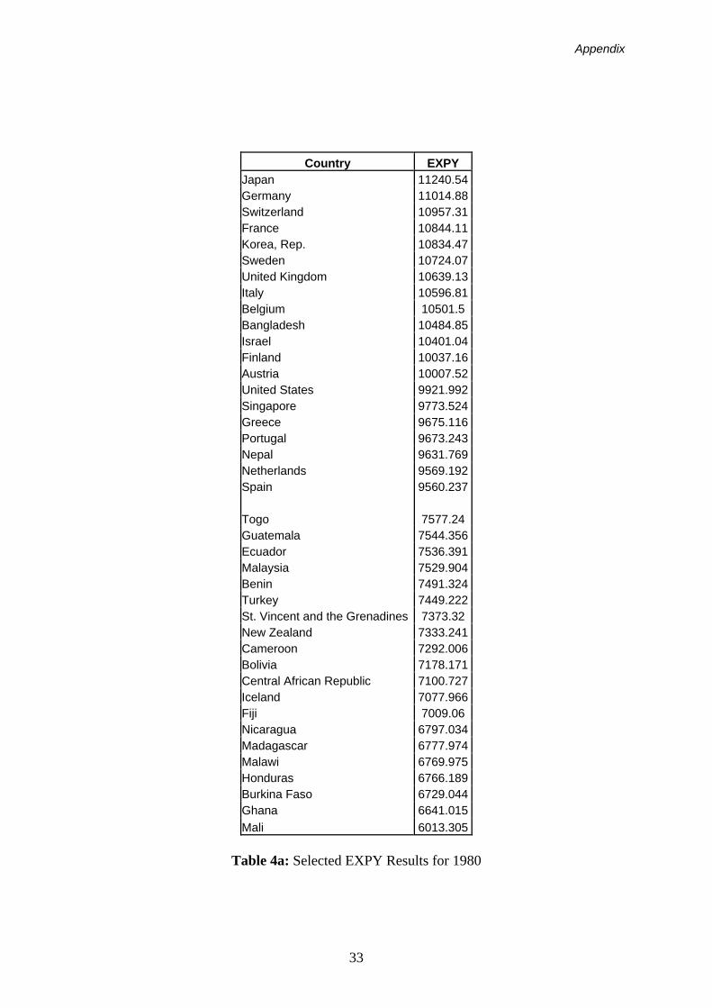
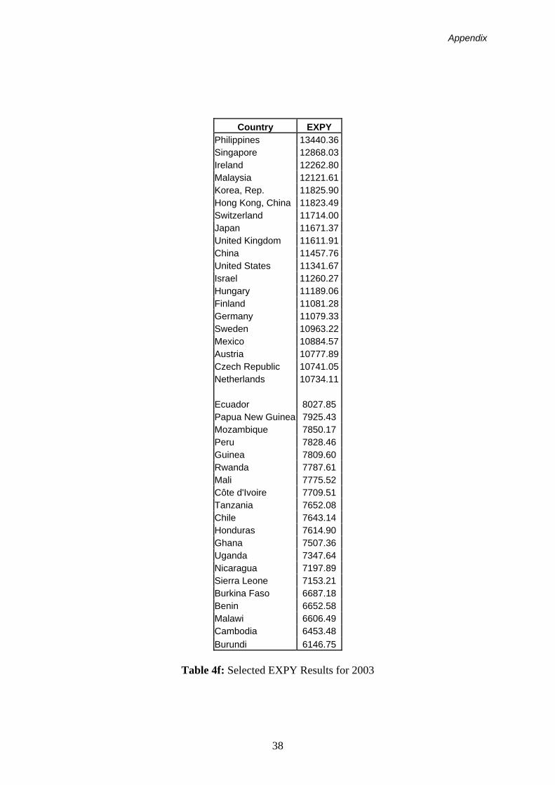
Moving onto the results for EXPY, the twenty highest and twenty lowest

EXPY values are shown for each year in Table 4. The global average for

EXPY is given in Table 3.

In each year, there are always some countries that have disproportionately

high EXPY values due to a reliance on one particular sector, thus not truly

reflecting a strong export composition. An example is that of Petro-states such

as Algeria, which in 1980 had 95% of its exports in Fuel. In 1980, Fuel was

ranked 3rd out of the nine sectors in terms of PRODY. Over the sample it

hovers around 6th or 7th in the rankings. Its PRODY value of between

$6,500million and $9,600million is nonetheless high enough that if

exceptionally large (often over 90%) proportions of exports lie within it, it will

lead to disproportionately high EXPY ratings. Countries such as Congo and

Trinidad & Tobago in 1980 and Nigeria in 2000 also have similar fuel-

dominated EXPY values. While these countries still do not feature towards the

top of the global EXPY rankings, this huge reliance on Fuel ensures that they

hover around the global average. Without Fuel having such a high PRODY

relative to other sectors prominent in countries of similar GDP, it would be

expected that the above-mentioned countries would feature at the bottom end

of the rankings, where countries of similar GDP per capita find themselves.

These other low-income countries are those that fit into the underlying

theoretical framework, with high percentages of their exports in the low

PRODY sectors such as Agricultural Raw Materials, Food and Ores & Metals.

An example of a lower-income country that has gained from its export

composition is Egypt, which in 1980 had 23% of its exports in Transport, 11%

in Travel, 9% in Computers and Communications, 9% in Agricultural Raw

Materials, 4% in Food, 6% in Manufacturing along with 36% in Fuel. This is an

example of a so-called “second world” country that has a well-diversified,

relatively highly productive export basket, managing to stay above the global

average from 1980 to 1995. Most European countries (along with the USA

and Canada) that appear in the top twenty in any given year are developed

countries that do not rely heavily on any given sector, but have quite high

proportions of their export basket in all the high-PRODY sectors. This is not

the case for Japan and Korea, and even Germany, which feature at the top of

the early EXPY ratings, however. These countries had up to 80% of their

19

Empirics

exports in Manufacturing in these early years, ensuring very high PRODY

values. The former is clearly the situation to which developing countries would

aspire in the long run. It is often, however, very difficult to move towards this

aim in the short run, due to what some commentators on export composition

and growth, such as Michaely (1977) and Tyler (1981), have termed the

“threshold effect”. This means that countries must attain a certain level of

development before they will see the gains from the composition of their

exports. One possible reason for this is that low income is usually correlated

with poor institutional quality and poor governance, two causes that are often

cited when explaining poor (in particular African) countries’ lack of economic

growth.

In the latter years of the sample, some unexpected countries are seen

towards the top of the EXPY tables. The majority of these countries have high

reliance on certain sectors, just as the Petro-states mentioned above, but in

this case the reliance is on more stable, less risk-bearing, higher PRODY

sectors such as High and Low-Tech Manufacturing. See Tables 4e and 4f for

rankings. In 2003, the Philippines had 61% of its exports in High-Tech

Manufacturing and 22% in Low-Tech Manufacturing, with all other sectors

taking up just 15%. These figures are almost identical for 2000. Singapore

shows similar trends, though without such an extreme concentration. The

same two sectors take up 69% in 1995, and 74% in 2000 and 2003.

Singapore also had higher GDP per capita and higher growth over 1995, 2000

and 2003, something which could be attributed to its higher level of economic

development, thus rendering it better able to exploit the gains from its exports.

Another example of a country that experienced rapid growth is

Malaysia. For the years 1990, 1995 and 2000, Malaysia averaged 9% growth.

This was one of the success stories of the “Asian Tiger” era, which also

included Singapore, as discussed above, along with Korea and Taiwan. As

can be seen from Tables 4c to 4e, in this period Malaysia features very high

up the list of EXPY values, as does Korea. From the results presented in this

paper, these countries can also be shown to confirm the importance of

diversifying exports into high productivity-enhancing activities in order to

achieve growth. A similar situation to the East Asian countries discussed

above exists for China, the major rising economic power. It is a source of

20

Empirics

major comment and debate, with Hausmann, Hwang and Rodrik (2005) giving

it special mention, and Rodrik (2006) focusing purely on China’s exports.

China has an EXPY value on a par with Switzerland, the UK, Germany,

France and Japan and the USA in the years 1995, 2000 and 2003. These are

countries that had income levels several times larger than China’s in these

years. On examination of the data which goes back quite a number of years,

the comparison can be made that China’s EXPY in the 1980’s was merely in

the middle of the global rankings, whereas it has shot up to rival that of the

major economic powers since the mid nineties. This time period is in line with

the period of China’s rapid and unprecedented economic growth, which is

causing such comment and analysis worldwide. Rodrik’s (2006) hypothesis is

that this rapid growth has been fuelled in no small way by China having an

export basket consisting of high-PRODY goods. This hypothesis is confirmed

by the findings in this paper, particularly when the comparison with China’s

earlier EXPY values is taken into account. Again, like Singapore, the

Philippines and Malaysia, the major reliance is on the Manufacturing sectors.

However, a closer look at the data reveals that China's export basket is

certainly moving in a healthy direction. In 1995, it had 8% in high-tech

Manufacturing and 68% in low-tech. By 2000 these figures had become 15%

and 64%, respectively, and by 2003 were 22% and 59%, respectively. As can

be seen, China has been moving into higher technology, more productivity-

enhancing, skill-intensive sectors as the economic boom has progressed. This

progression can be used as part explanation for this rapid growth, as argued

by Rodrik (2006).

At the opposite end of the rankings, examples such as that of Benin

can be cited, with 26% of its exports in Agricultural Raw Materials and 46% in

food in 2003. These are the low-skill sectors that the Heckscher-Ohlin

framework associates with low-income countries, and are those that offer the

least possibilities for knowledge spillovers and other positive externalities into

the domestic economy. Similar situations exist for the majority of countries

cited in the bottom twenty listed in Tables 4a to 4f. A surprising entry in this

list is Iceland for 2000. Despite having an impressive GDP per capita of some

$28,000, Iceland's export basket is not composed of products that would be

expected for such an income. The main driver of the low EXPY is Food, taking

21

Empirics

up 44%, while Ores & Metals take up 13%, with both Manufacturing sectors

and Insurance and Financial Services accounting for just 10% altogether.

Similar anecdotal evidence is available for other primary-oriented exporters

such as Argentina in 1985 and New Zealand in 1990. These countries were

also plagued with low growth over the period, with New Zealand growing by

less than 1% up until 2000, when it catapulted to 4%. Argentina in fact

experienced negative growth in each year of the sample since 1985, although

this country has had many other well-documented problems regarding its

macroeconomic management. These examples can be tied in with the

literature on the natural resource curse and “Dutch disease”

The impact of EXPY on growth has been presented in an anecdotal

form in this section, with many examples given of countries that have grown in

tandem with increased sophistication of their export baskets. This relationship

will be tested formally in the next section using panel regression analysis.

22

Growth Regressions

4 GROWTH REGRESSIONS 4.1 Data and Methodology Attention will now be turned to the relationship between EXPY and growth.

For the growth regressions, the y-variable is GDP growth (annual %). This

series was also taken from the WDI (2005) database, along with population

growth (annual %). As an indicator for educational attainment, the percentage

of the over 25 population for whom secondary education is the highest level

achieved is used. This was obtained from Barro and Lee’s “International Data

on Educational Attainment: Updates and Implications” published in 2000. The

share of investment in GDP is also included in the growth regression. This

data was obtained from the Penn World Table database. As the data came

from different sources, it was inevitable that certain countries would have

missing observations in some of the series. As a result, the final sample size

for the balanced panel is 50 countries, for the years 1980, 1985, 1990, 1995

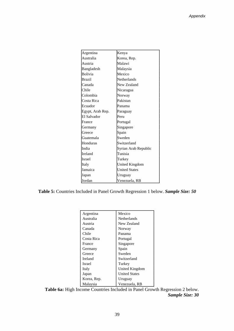
and 2000, thus leading to 250 observations. A list of the countries included in

the panel is given in Table 5.

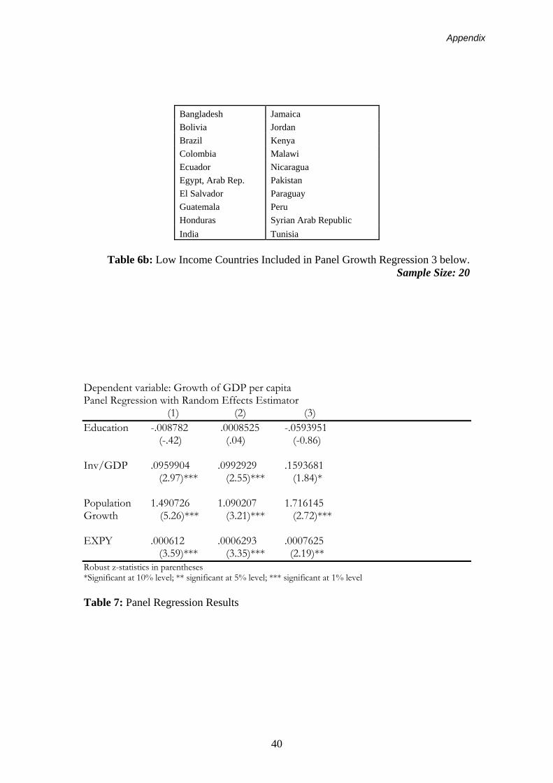
4.2 Regressions and Results A panel regression is carried out using the random effects estimator with GDP

growth (annual %) as the dependent variable, and education,

investment/GDP, population growth and EXPY as the independent variables.

This is referred to as Regression 1 in the results, which are given in Table 7.

EXPY enters into this panel with a positive impact of 0.00061, significant at

the 1% level. This means that a one-unit increase in EXPY leads to a 0.00061

of a per cent increase in growth. Considering EXPY values average between

$8,000 and $10,000 (where the unit is millions of dollars), a more relevant

observation would be that a 1,000-unit increase in EXPY (equating to in and

around a 10% increase) leads to approximately a three fifths of a percent

increase in growth. This is significant at the one percent level. Increases (and

decreases) of over 500 units have occurred regularly across the 5-year

periods in the sample studied, meaning that this is not a negligible impact.

Aside from EXPY, the education variable shows no significant effect on

23

Growth Regressions

growth in this sample, while population growth and the investment to GDP

ratio show the expected positive effects, significant at the one percent level.

The balanced panel was then divided into two sub-samples, high and

low-income countries. These are defined by the WDI (2005). The sample of

high-income countries comprised those defined as “high-income, OECD”,

“high-income, non-OECD” and “upper middle income”, with a sample size of

30. The low-income sub sample comprised countries defined as “lower middle

income” and “low-income”, with a sample size of 20. The division of the

countries between these two samples is given in Tables 6a and 6b. The aim

was to investigate whether or not some of the results could be attributed to a

strong influence from one of the income groups. The same regression as

before was carried out with the regression of the high-income countries

referred to as Regression 2 and the regression of low-income countries

referred to as Regression 3. Results are given in Table 7.

For the sub-sample of high-income countries, the impact of EXPY

remains almost identical at 0.63 of a percent for a 1000-unit increase in

EXPY. This is significant at the one percent level. A more interesting result is

that for the sub-sample of lower income countries. For this sample the impact

of EXPY is significant only at the 5% level, but has an increased effect of

three-quarters of a percent on growth for a 1000-unit increase. Population

growth is significant at the 1% level for both sub-samples, with there being a

stronger effect for lower income countries, as would be expected. The

investment to GDP ratio is significant at the 1% level for rich countries, while

only at the 10% level for lower income countries. It also has a greater impact

on lower income countries. The importance of the results found in this section

should not be underestimated. It has been found that export sophistication

can have growth-enhancing effects, with countries that increase the

sophistication of their export basket by roughly 10-12% standing to increase

growth by three fifths of a percent. A more interesting observation is that the

effect of EXPY on growth is compounded when low-income countries are

viewed, with the effect rising to three-quarters of a percent on growth. This

observation for low-income countries has interesting connotations for

economic development, leading to policy implications that should be the

subject of further debate and discussion.

24

A Look at the Irish Story

25

Conclusion

5 CONCLUSION The export led growth (ELG) hypothesis states that an increase in the volume

of exports can drive economic growth. In this paper, the principal aim was to

go further than this, and test whether it was the composition of exports, rather

than the volume, that was more important for economic growth. Reasons cited

for why this may be the case included the fact that exporting in more

sophisticated sectors allows the transmission of knowledge and skills into the

domestic economy through exposure to foreign competition and more efficient

modern business practices. These competitive pressures spur innovation and

technological advancement at home, leading to an increased skill level in the

domestic economy. The explanation for why a country exports the type of

products that it does was given through the Heckscher-Ohlin framework,

whereby countries produce and export goods for which they have a

comparative endowment advantage. Countries that have high capital-labour

and high skilled-unskilled labour ratios are typically rich, developed countries.

It is for this reason that the weighted average of the GDP per capita of all

countries exporting a product is used as a proxy for product sophistication in

this paper. This weighted average is known as PRODY. The weights in

PRODY calculation correspond to revealed comparative advantage in the

particular sector.

PRODY was calculated for 11 sectors across 6 different years. The

results were in line with the underlying theoretical framework, with the highest

PRODY figures being for sectors exported predominantly by developed

countries such as High-Tech Manufacturing and Insurance and Financial

Services. The lowest PRODY values were for primary sectors, which typically

take up a higher share of less developed countries’ exports.

The sophistication level of a country’s export basket is then calculated

simply as the weighted average of the PRODY for each sector, where the

weights are the value share of each sector in the country’s exports. This gives

an index referred to as EXPY. The results section in this study shows that

developed countries such as Japan, Germany, France, USA, UK and in later

years Ireland, take their place towards the top of global EXPY rankings. It can

also be seen, interestingly, that growing countries such as China, Singapore,

26

Conclusion

Malaysia and the Philippines have also been toward the top of the global

tables over the years. This surprising result, given these countries’ GDP per

capita levels, can be viewed as evidence that a high EXPY level can be an

engine for economic growth.

To test this anecdotal evidence more formally, in Section 4 panel

growth regressions were reported with EXPY included as an explanatory

variable along with the standard education, population growth and investment

variables. EXPY entered into this model with a positive effect, significant at

the one percent level. An increase of roughly 10% in EXPY increases GDP

growth by three fifths of a percentage point. This formalized the hypothesis of

the paper. Even more interestingly, when the countries of the panel were

divided into poor and rich countries, the effect stayed identical for rich

countries, and increased further to three quarters of a percentage point for the

poor countries of the sample. These important findings have implications for

thinking in economic development, in that perhaps underdeveloped countries

need to be encouraged to diversify their export baskets towards more

sophisticated sectors in order to move away from their current economic

status. Clearly, there is a great deal of complexity involved in such a move,

and much investment in capital, human and otherwise, required, which should

be the subject of much discussion in further research.

An economy must align its export composition so as to be able to latch

onto highly sophisticated export sectors. In the case where the export sector

is reliant on foreign investment, it must also however have the systems

available for learning to take place so that knowledge diffusion can occur into

the domestic economy. It seems that the combination of these two is the

ideal, yet difficult-to-attain, situation for a country to be in, in order to ensure

that the gains from its exports are converted into increases in economic

growth. Such a strategy should be adopted to help sustain economic growth,

particularly in the developing countries of the world.

27

Bibliography

BIBLIOGRAPHY Abou-Stait, F. (2005) Are exports the engine of economic growth? An application of cointegration and causality analysis for Egypt, 1977-2003. African Development Bank Economic Research Working Papers, no. 76. Amable, B. (2000) International Specialisation and Growth. Structural Change and Economic Dynamics, 11:4, 413-432. Awokuse, T.O. (2002) Is the Export-Led Growth hypothesis valid for Canada? Department of Food and Research Economics, University of Delaware, FREC, SP 02-01. Balassa, B. (1978) Exports and economic growth: further evidence. Journal of Development Economics 5, 181–9. Balassa, B. (1981) The Newly Industrializing Countries in the World Economy. New York: Pergamon Press. Barro, R.J. and Lee, J.W. (2000) International Data on Educational Attainment: Updates and Implications. CID Working Paper No. 42, April 2000. Burkett, J.P. (2000) Cones of diversification in a model of international comparative advantage. Journal of International Trade & Economic Development, 9:2, 193–211. Burney, N.A. (1996) Exports and economic growth: evidence from cross country analysis. Applied Economics Letters, 3, 369–73. Crespo-Cuaresma, J. and Wörz, J. (2005) On export composition and growth. Review of World Economics/Weltwirtschaftliches Archiv, 141, 33-49. Darrat, A.F. (1986) Trade and development: the Asian experience. Cato Journal, 6, 695–9. Davis, D.R. (1995) Intra-industry trade: a Heckscher–Ohlin–Ricardo approach, Journal of International Economics 39, pp. 201–226. Doyle, E., (1998) Export-output causality: the Irish case 1953-93, Atlantic Economic Journal, 26: 2, 147-62. Evenson, R. E. and Westphal, L.E. 1995. Technological Change and Technology Strategy, in Hollis B. Chenery and T.N. Srinivasan, Eds. Handbook of Development Economics, Vol. 3., Amsterdam: North-Holland, 2211- 2298. Feder, G. (1983) On Exports and Economic Growth. Journal of Development Economics, 12, 59-73.

28

Bibliography

Findlay, C. and Watson, A. (1996) Economic growth and trade dependency in China. DP #96/5, Chinese Economies Research Centre, University of Adelaide. Fosu, A.K. (1990) Exports and economic growth: the African case. World Development, 18, 831–5.

Frankel, J.A. and Romer, D. (1999) Does Trade Cause Growth? The American Economic Review, 89: 3. 379-399. Giles, J.A., and Williams, C.L. (2000) Export-Led Growth: a survey of the empirical literature and some non-causality results. Part 1. Journal of International Trade & Economic Development, 9:3, 261–337.

Gorg, H. and Strobl, E. (2005) Spillovers from foreign firms through worker mobility: an empirical investigation. Scandinavian Journal of Economics, 107: 4, 693-709. Greenaway, D., Morgan, W. and Wright, P. (1999) Exports, export composition and growth. Journal of International Trade and Economic Development, 8:1, 41-51. Grabowski, R., Sharma, S.C. and Dhakal, D. (1990) Exports and Japanese economic development. Economics Letters, 32, 127–32. Harrigan, J. (1999) Estimation of Cross-Country Differences in Industry Production Functions.” Journal of International Economics 47, 267–93. Harrigan, J. (1997a) Cross-Country Comparisons of Industry Total Factor Productivity: Theory and Evidence. Research Paper no. 9734. New York: Fed. Reserve Bank, November 1997. Harrigan, J. (1997b) Technology, Factor Supplies, and International Specialization: Estimating the Neoclassical Model.” American Economic Review 87 475–94. Hatzichronoglou, T. (1997) Revision of the high-technology sector and product classification, Paris: OECD, STI Working Papers, 1997/2. Hausmann, R., Hwang, J. and Rodrik, D.(2005) What You Export Matters. KSG Working Paper No. RWP05-063. Hausmann, R. and Rodrik, D. (2003) Economic Development as Self-Discovery. Journal of Development Economics, December 2003. Henriques, I. and Sadorsky, P. (1996) Export-Led Growth or Growth-driven Exports? The Canadian Case. Canadian Journal of Economics, 12:3, 540-555. Herzer, D., Nowak-Lehmann, F. and Siliverstovs, B. (2004) Export-Led Growth in Chile: Assessing the Role of Export Composition in Productivity

29

Bibliography

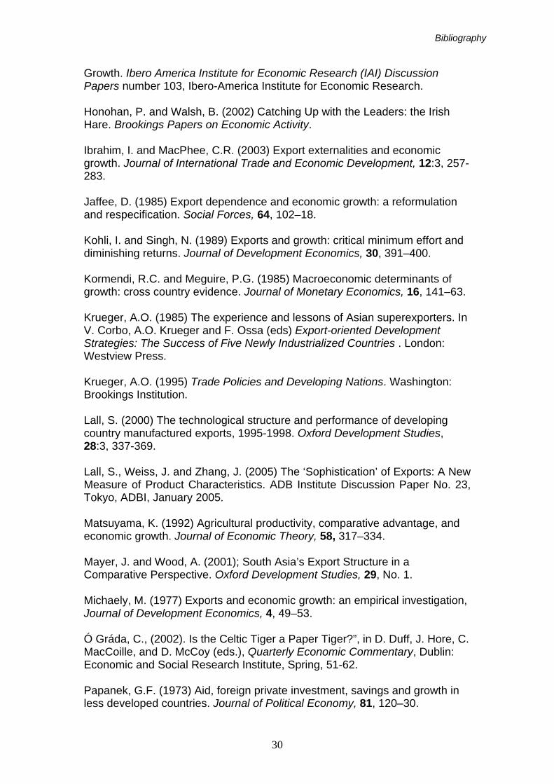
Growth. Ibero America Institute for Economic Research (IAI) Discussion Papers number 103, Ibero-America Institute for Economic Research. Honohan, P. and Walsh, B. (2002) Catching Up with the Leaders: the Irish Hare. Brookings Papers on Economic Activity. Ibrahim, I. and MacPhee, C.R. (2003) Export externalities and economic growth. Journal of International Trade and Economic Development, 12:3, 257-283. Jaffee, D. (1985) Export dependence and economic growth: a reformulation and respecification. Social Forces, 64, 102–18. Kohli, I. and Singh, N. (1989) Exports and growth: critical minimum effort and diminishing returns. Journal of Development Economics, 30, 391–400. Kormendi, R.C. and Meguire, P.G. (1985) Macroeconomic determinants of growth: cross country evidence. Journal of Monetary Economics, 16, 141–63. Krueger, A.O. (1985) The experience and lessons of Asian superexporters. In V. Corbo, A.O. Krueger and F. Ossa (eds) Export-oriented Development Strategies: The Success of Five Newly Industrialized Countries . London: Westview Press. Krueger, A.O. (1995) Trade Policies and Developing Nations. Washington: Brookings Institution. Lall, S. (2000) The technological structure and performance of developing country manufactured exports, 1995-1998. Oxford Development Studies, 28:3, 337-369. Lall, S., Weiss, J. and Zhang, J. (2005) The ‘Sophistication’ of Exports: A New Measure of Product Characteristics. ADB Institute Discussion Paper No. 23, Tokyo, ADBI, January 2005. Matsuyama, K. (1992) Agricultural productivity, comparative advantage, and economic growth. Journal of Economic Theory, 58, 317–334. Mayer, J. and Wood, A. (2001); South Asia’s Export Structure in a Comparative Perspective. Oxford Development Studies, 29, No. 1. Michaely, M. (1977) Exports and economic growth: an empirical investigation, Journal of Development Economics, 4, 49–53. Ó Gráda, C., (2002). Is the Celtic Tiger a Paper Tiger?”, in D. Duff, J. Hore, C. MacCoille, and D. McCoy (eds.), Quarterly Economic Commentary, Dublin: Economic and Social Research Institute, Spring, 51-62. Papanek, G.F. (1973) Aid, foreign private investment, savings and growth in less developed countries. Journal of Political Economy, 81, 120–30.

30

Bibliography

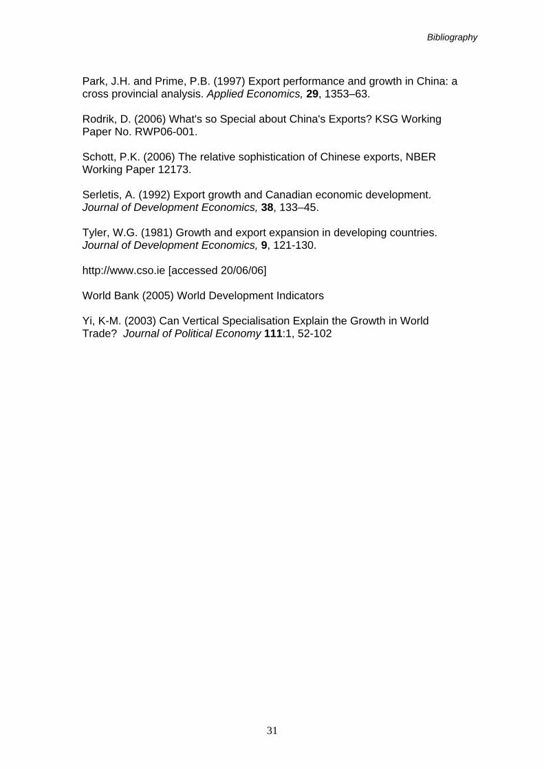
Park, J.H. and Prime, P.B. (1997) Export performance and growth in China: a cross provincial analysis. Applied Economics, 29, 1353–63. Rodrik, D. (2006) What's so Special about China's Exports? KSG Working Paper No. RWP06-001. Schott, P.K. (2006) The relative sophistication of Chinese exports, NBER Working Paper 12173. Serletis, A. (1992) Export growth and Canadian economic development. Journal of Development Economics, 38, 133–45. Tyler, W.G. (1981) Growth and export expansion in developing countries. Journal of Development Economics, 9, 121-130. http://www.cso.ie [accessed 20/06/06] World Bank (2005) World Development Indicators Yi, K-M. (2003) Can Vertical Specialisation Explain the Growth in World Trade? Journal of Political Economy 111:1, 52-102

31

Appendix

APPENDIX

Year Sample Size1980 80 1985 81 1990 77 1995 104 2000 117 2003 110

Table 1: Sample Size by Year

Year 1980 1985 1990 1995 2000 2003 Sector Agri. Raw Materials 5083.87 6682.73 6299.65 6474.05 6139.13 5331.75Food 5855.20 6175.54 5870.32 6130.19 6772.26 5792.91Fuel 8030.03 7463.18 6552.56 8964.72 8530.52 9343.17Ores & Metals 6747.52 7463.70 6659.71 7760.63 7038.08 6502.98Manufacturing 11553.56 11899.33 12122.81 N/A N/A N/A High-Tech Manuf. N/A N/A N/A 17321.66 17093.29 16017.65Low-Tech Manuf. N/A N/A N/A 11845.26 12292.71 10555.93Computers & Comms. 17263.81 9400.49 9715.12 9109.63 11827.83 12904.14Insurance & Financial 7489.70 9067.62 11406.31 12569.59 14072.13 16579.22Transport 8280.93 8863.63 8748.92 8958.21 10793.94 10191.14Travel 7395.41 8147.23 8473.82 8536.35 9630.41 8278.30

Table 2: PRODY Results by Year and Sector

Year EXPY 1980 8435.151985 8737.971990 8942.591990 9428.862000 10386.082003 9436.22

Table 3: Global EXPY Average by Year

32

Appendix

Country EXPY Japan 11240.54Germany 11014.88Switzerland 10957.31France 10844.11Korea, Rep. 10834.47Sweden 10724.07United Kingdom 10639.13Italy 10596.81Belgium 10501.5Bangladesh 10484.85Israel 10401.04Finland 10037.16Austria 10007.52United States 9921.992Singapore 9773.524Greece 9675.116Portugal 9673.243Nepal 9631.769Netherlands 9569.192Spain 9560.237 Togo 7577.24Guatemala 7544.356Ecuador 7536.391Malaysia 7529.904Benin 7491.324Turkey 7449.222St. Vincent and the Grenadines 7373.32New Zealand 7333.241Cameroon 7292.006Bolivia 7178.171Central African Republic 7100.727Iceland 7077.966Fiji 7009.06Nicaragua 6797.034Madagascar 6777.974Malawi 6769.975Honduras 6766.189Burkina Faso 6729.044Ghana 6641.015Mali 6013.305

Table 4a: Selected EXPY Results for 1980

33

Appendix

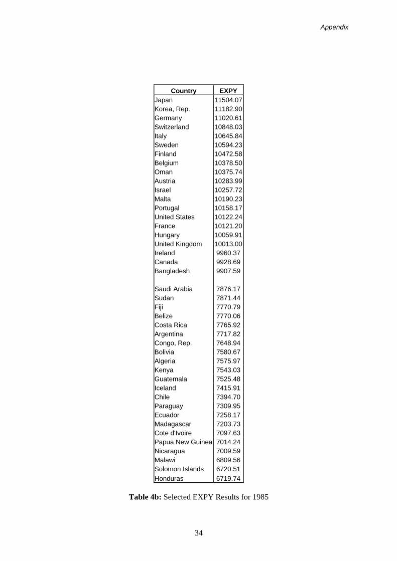
Country EXPY Japan 11504.07Korea, Rep. 11182.90Germany 11020.61Switzerland 10848.03Italy 10645.84Sweden 10594.23Finland 10472.58Belgium 10378.50Oman 10375.74Austria 10283.99Israel 10257.72Malta 10190.23Portugal 10158.17United States 10122.24France 10121.20Hungary 10059.91United Kingdom 10013.00Ireland 9960.37Canada 9928.69Bangladesh 9907.59 Saudi Arabia 7876.17Sudan 7871.44Fiji 7770.79Belize 7770.06Costa Rica 7765.92Argentina 7717.82Congo, Rep. 7648.94Bolivia 7580.67Algeria 7575.97Kenya 7543.03Guatemala 7525.48Iceland 7415.91Chile 7394.70Paraguay 7309.95Ecuador 7258.17Madagascar 7203.73Cote d'Ivoire 7097.63Papua New Guinea 7014.24Nicaragua 7009.59Malawi 6809.56Solomon Islands 6720.51Honduras 6719.74

Table 4b: Selected EXPY Results for 1985

34

Appendix

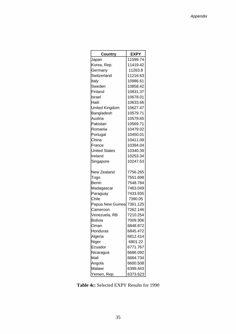
Country EXPY Japan 11599.74Korea, Rep. 11419.42Germany 11263.8Switzerland 11216.63Italy 10986.61Sweden 10858.42Finland 10831.37Israel 10678.01Haiti 10633.66United Kingdom 10627.47Bangladesh 10579.71Austria 10579.65Pakistan 10569.71Romania 10479.02Portugal 10450.01China 10411.09France 10394.04United States 10340.39Ireland 10253.34Singapore 10247.53 New Zealand 7756.265Togo 7551.698Benin 7548.784Madagascar 7463.049Paraguay 7433.935Chile 7390.05Papua New Guinea 7361.125Cameroon 7262.146Venezuela, RB 7210.254Bolivia 7009.306Oman 6848.872Honduras 6845.472Algeria 6812.414Niger 6801.22Ecuador 6771.767Nicaragua 6686.092Mali 6684.734Angola 6600.508Malawi 6399.443Yemen, Rep. 6373.623

Table 4c: Selected EXPY Results for 1990

35

Appendix

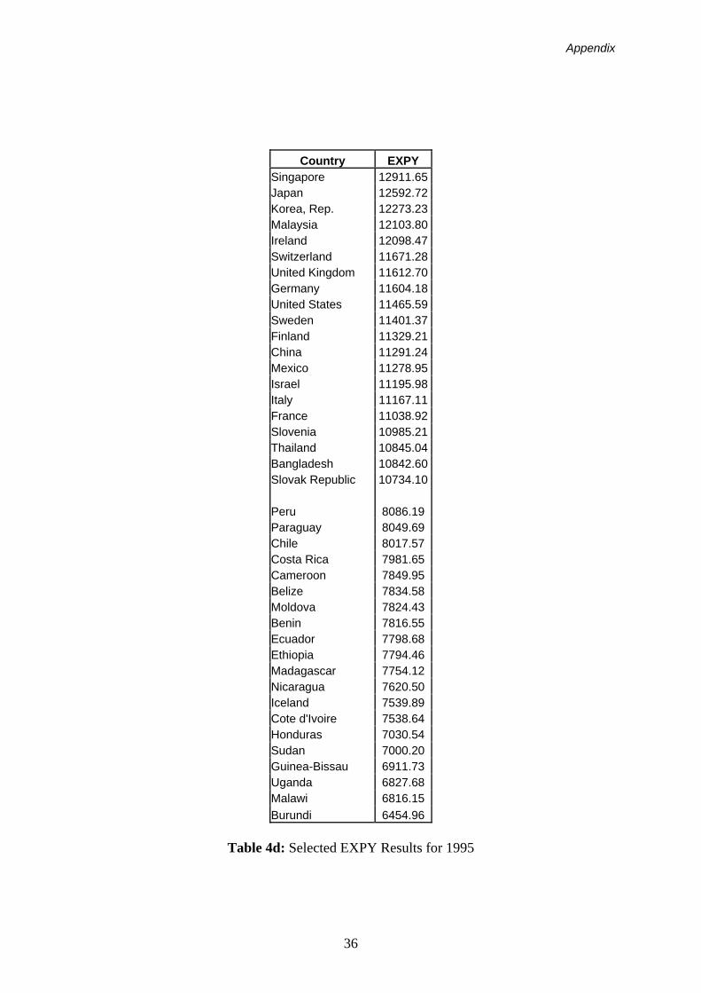
Country EXPY Singapore 12911.65Japan 12592.72Korea, Rep. 12273.23Malaysia 12103.80Ireland 12098.47Switzerland 11671.28United Kingdom 11612.70Germany 11604.18United States 11465.59Sweden 11401.37Finland 11329.21China 11291.24Mexico 11278.95Israel 11195.98Italy 11167.11France 11038.92Slovenia 10985.21Thailand 10845.04Bangladesh 10842.60Slovak Republic 10734.10 Peru 8086.19Paraguay 8049.69Chile 8017.57Costa Rica 7981.65Cameroon 7849.95Belize 7834.58Moldova 7824.43Benin 7816.55Ecuador 7798.68Ethiopia 7794.46Madagascar 7754.12Nicaragua 7620.50Iceland 7539.89Cote d'Ivoire 7538.64Honduras 7030.54Sudan 7000.20Guinea-Bissau 6911.73Uganda 6827.68Malawi 6816.15Burundi 6454.96

Table 4d: Selected EXPY Results for 1995

36

Appendix

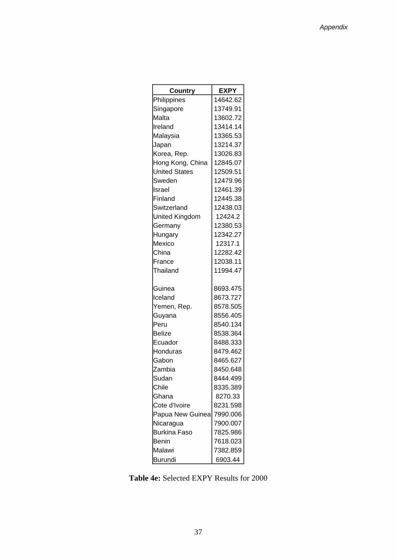
Country EXPY Philippines 14642.62Singapore 13749.91Malta 13602.72Ireland 13414.14Malaysia 13365.53Japan 13214.37Korea, Rep. 13026.83Hong Kong, China 12845.07United States 12509.51Sweden 12479.96Israel 12461.39Finland 12445.38Switzerland 12438.03United Kingdom 12424.2Germany 12380.53Hungary 12342.27Mexico 12317.1China 12282.42France 12038.11Thailand 11994.47 Guinea 8693.475Iceland 8673.727Yemen, Rep. 8578.505Guyana 8556.405Peru 8540.134Belize 8538.364Ecuador 8488.333Honduras 8479.462Gabon 8465.627Zambia 8450.648Sudan 8444.499Chile 8335.389Ghana 8270.33Cote d'Ivoire 8231.598Papua New Guinea 7990.006Nicaragua 7900.007Burkina Faso 7825.986Benin 7618.023Malawi 7382.859Burundi 6903.44

Table 4e: Selected EXPY Results for 2000

37

Appendix

Country EXPY Philippines 13440.36Singapore 12868.03Ireland 12262.80Malaysia 12121.61Korea, Rep. 11825.90Hong Kong, China 11823.49Switzerland 11714.00Japan 11671.37United Kingdom 11611.91China 11457.76United States 11341.67Israel 11260.27Hungary 11189.06Finland 11081.28Germany 11079.33Sweden 10963.22Mexico 10884.57Austria 10777.89Czech Republic 10741.05Netherlands 10734.11 Ecuador 8027.85Papua New Guinea 7925.43Mozambique 7850.17Peru 7828.46Guinea 7809.60Rwanda 7787.61Mali 7775.52Côte d'Ivoire 7709.51Tanzania 7652.08Chile 7643.14Honduras 7614.90Ghana 7507.36Uganda 7347.64Nicaragua 7197.89Sierra Leone 7153.21Burkina Faso 6687.18Benin 6652.58Malawi 6606.49Cambodia 6453.48Burundi 6146.75

Table 4f: Selected EXPY Results for 2003

38

Appendix

Argentina Kenya Australia Korea, Rep. Austria Malawi Bangladesh Malaysia Bolivia Mexico Brazil Netherlands Canada New Zealand Chile Nicaragua Colombia Norway Costa Rica Pakistan Ecuador Panama Egypt, Arab Rep. Paraguay El Salvador Peru France Portugal Germany Singapore Greece Spain Guatemala Sweden Honduras Switzerland India Syrian Arab Republic Ireland Tunisia Israel Turkey Italy United Kingdom Jamaica United States Japan Uruguay Jordan Venezuela, RB

Table 5: Countries Included in Panel Growth Regression 1 below. Sample Size: 50

Argentina Mexico Australia Netherlands Austria New Zealand Canada Norway Chile Panama Costa Rica Portugal France Singapore Germany Spain Greece Sweden Ireland Switzerland Israel Turkey Italy United Kingdom Japan United States Korea, Rep. Uruguay Malaysia Venezuela, RB

Table 6a: High Income Countries Included in Panel Growth Regression 2 below. Sample Size: 30

39

Appendix

Bangladesh Jamaica Bolivia Jordan Brazil Kenya Colombia Malawi Ecuador Nicaragua Egypt, Arab Rep. Pakistan El Salvador Paraguay Guatemala Peru Honduras Syrian Arab Republic India Tunisia

Table 6b: Low Income Countries Included in Panel Growth Regression 3 below.

Sample Size: 20 Dependent variable: Growth of GDP per capita Panel Regression with Random Effects Estimator (1) (2) (3) Education -.008782 .0008525 -.0593951 (-.42) (.04) (-0.86) Inv/GDP .0959904 .0992929 .1593681 (2.97)*** (2.55)*** (1.84)* Population 1.490726 1.090207 1.716145 Growth (5.26)*** (3.21)*** (2.72)*** EXPY .000612 .0006293 .0007625 (3.59)*** (3.35)*** (2.19)** Robust z-statistics in parentheses *Significant at 10% level; ** significant at 5% level; *** significant at 1% level Table 7: Panel Regression Results

40