Exponential Distribution and the Process of Radioactive Decay

Chapter 6

Exponential Distribution andthe Process of RadioactiveDecay

The problem of radioactive decay is one of the simplest examples which show theconnection between deterministic models and stochastic approach. We emphasize thatthe stochastic model is not an alternative to the deterministic approach, rather it is ageneralization: a satisfactory stochastic model gives a derivation for the deterministicmodel and more.

The deterministic model for radioactive decay��

is a simple linear differ-ential equation ��

��

where��

is the number of atom�

and�

is the rate of decay. To solve this ODE withinitial condition

�� , we have�� ! #"%$(6.1)

If we observe the decay of atom�

one by one, then one realizes that the time atwhich

�transforming to

�&�is random. Hence the microscopic process of radioactive

decay has to be modeled by a stochastic model. Specifically, if we denote ' as thelifetime of

�, ' is a continuous, positive random variable. How do we determine the

probability distribution for ' ? The basic assumption for the stochastic model is thatthe decay of

�, as a random event, is independent of the time the atom being in

�. In

other words, the conditional probability

(&)+*-,+. '0/ !13254 '0/ %6 � (&)7*-,8. '0/ 296�$

As we will soon see, this assumption is sufficient to determine the probability distribu-tion of ' . It is known as the exponential distribution.

35

36 Hong Qian/AMATH 423

6.1 Exponential Distribution

The exponential distribution has the very important property known as memoriless:

(&)7*-,8. '0/ !132 4 '0/ %6 �� "�� ! #" � � �! �� (&)7*-,8. '0/ 296�$

In fact, this nice property is the defining character of the exponential distribution. Con-sider a RV ' with

(&)7*-,8. '0/ !13296 � (&)7*-,8. '0/ 9132 4 '0/ %6 (&)7*-,8. '0/ %6� (&)7*-,8. '0/ 296 (&)7*-,8. '0/ %6�$

Let �� (&)7*-,8. '0/ %6 then �� 1 2 � � �� 2 �

�� 1 2 � � �� 2 � � � �� 2 �

��

� � 2 � � 2 � � ��

�� i.e., ' is exponential

(&)+*-,+. '�� %6 �� ! #" $ (6.2)

6.2 Microscopic versus Macroscopic Models

What is the relation between Eqn. 6.1 and Eqn. 6.2. Afterall, both are mathematicalmodels for the radioactive decay. The relation lies upon the a system of

number of

independent atoms with very large

. From Eqn. 6.2, we note that at any time , the

atom is still in�

with probability� �! �"

and in�&�

with probability � � � �� " . This is abinary distribution. Hence, for

��iid, we have

(&)7*-,8.�� " �� 6 � ��

� � �� #"�� "! �"�# �� (6.3)

where RV� "

is the number of atoms being�

at time t. So the expectation and variancefor

� "are

$&% � "(' � �� " )+* ),% � "-' � �� "�� "! which indicates that Eqn. 6.1 is simply the mean of the

� ". The stochastic model,

however, also provide an estimation for the variance. It is shown that for a large �

onthe order of �

��. �, the relative broadness of the distribution

Applied Stochastic Analysis 37

) * ) % � " '$&% � "(' . �� $

This proves that the deterministic model is a very good approximation if one deals withlarge number of atoms, i.e., macroscopic. It also shows when studying system of onlya few number of atoms (microscopic), the stochastic model is more general.


Chapter 7

Poisson Processes

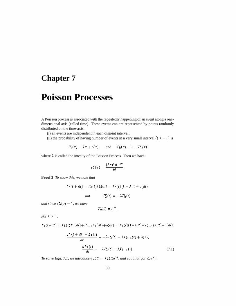
A Poisson process is associated with the repeatedly happening of an event along a one-dimensional axis (called time). These evetns can are represented by points randomlydistributed on the time-axis.

(i) all events are independent in each disjoint interval;(ii) the probability of having number of events in a very small interval

� 1 � � is

(�� 1 * � � � and( �� (��

where�

is called the intesity of the Poisson Process. Then we have:

(�� ! �� $

Proof 3 To show this, we note that

( � �� 91 �� ( � �� ( � � � �� ( � �� % � � � � 1 * �� '�� ( �� ( � ��

and since( � �� , we have ( �� " $

For�� ,

(� � %1&� �� (�� ( � �� 1 (� � � (�� %1 * � � �� (�� 1 (�� %1 * �� ( � �� !1 �� ( � �� (� � �� 1 � (�� 1 * � � �

� (� � �� (�� 1 � (� � � �� $(7.1)

To solve Eqn. 7.1, we introduce �� (� �� " , and equation for �

� ��:

39


� ��

�� ( � �� 7 �"91 � � � ��

� �� 1 � � � � �� 1 � � ��

with condition ��

. We therefore have

��

� � �� and

( � �� $

7.1 Properties of a Poisson Process

There are two aspects of a Poisson process: the distribution for the time intervalsand the distribution for the corresponding counting process.

(i) if � � , � . , ..., �� are independent Poisson random variables, then

� � � � 1 � . 1 $ $ $81 ��is still Poisson.

Homework. Try to use the method of generating function to show that the randomsum of � � 1 � . 1 $ $ $+1 �� where � is a Poisson RV with mean

�, and

�’s are iid binary RVs with

(&)7*-,8.�� 6 �� and

(&)7*-,8.�� 6 � � � � , is still Poisson.

(ii) The waiting distribution. What is the probability distribution of first arrivingevent? Let’s denote the time by a RV � � , then

(&)7*-,8. � � � %6 � � � (&)7*-,8. � � / %6� � � (&)7*-,8.�� " � � 6� � � � �! #"

where� "

is the number of event before time

(counting process). The pdf for � � isobtained by derivative: � � � �� " $Hence, Poisson process is intimately related to the exponential distribution.

Similarly, let’s consider � � :(&)7*-,8. � � � %6 � � � (&)7*-,8. � � / %6� � � (&)7*-,8.�� " � �� 6

� � ��

� � �� "� � $


Again, differentiation with respect to , we have pdf:

�� (&)7*-,8. � � � %6 � �

� � ��

� � � � ��

�� ! �"

� ��

� � .� ��

� � � �� "

� � 1 � � ��

� � � �� ! �"

� �� "� ��

which is called gamma distribution. When� � � , � � is called exponentially dis-

tributed.(iii) We now show that gamma distribution of order

�is just the sum of

�exponential

distributions:

� � � � � 1 � � . � � � � 1 � �� . �91 $ $ $+1 � � � � � � � � � where the waiting times for

�th event �� are independent.

Proof 4 We first find out the characteristic function for gamma distribution:�� ! �"� � � � � �� " ��

� 1 �� "

� �� 1 �� .� �� " ��

� $ $ $� �

� 1 �� $Note that �

� 1 �� " � � �� " �� is the characteristic function of an exponential distribution.

(iv) The mean of the gamma distribution is�� 1 �� 1 ��

as expected. �� is the mean waiting time.

7.2 Uniform Distribution and Poisson Processes

If points generated by a Poisson process are labeled on a time axis, what is theirdistribution? The answer is they are uniform with density

�. This is not a very intuitive


result. The key is that the statement is conditioned on a fixed total number of events inan interval !

Let � � , � . , ... be the occurrence times in a Poisson process of intensity�

. Con-ditioned on

� " � � , the random variable � � , � . , ..., � � are uniformly distributed onthe interval

% � �� .We prove a simplified version of this result: � �� . We know joint pdf for RVs � �

and � . :(&)7*-,8. � � �� 91 �� . � � 1 � � 6 � � . ��! #" �� "�� / ��

therefore,

(&)7*-,8. � � � � 1 �� . � � 6 � �� . � �� " � �� "�� ! �� / �� $

Hence,

(&)+*-,+. � � �� 91 �� #4 � . � � 6 � (&)7*-,8. � � � � 91 � � . � � 6(&)+*-,+. � . � � 6� � � �

� � � � � � �! �� ! ��

��

��

� � � � $

This is a uniform distribution on% � � � . Note that if without the condition,

(&)7*-,8. � � �� 91 �� %6 � � � �� " �� $

This result shows how important the condition is to a probabilistic problem.

7.3 Poissonization

Poisson processes not only offer models for biological problems, they also providean approach to some problems that at first sight seem totally unrelated. Formulatingsuch problems in terms of Poisson processes is called Poissonization. The relation-ship between a Poisson process and the uniform distribution is the foundation for thisapproach.

Let’s consider, for instance, computing the expectation$ � ��

of the total numberof children

� �� born to a couple who stop reproducing when they reach their goal of

at least,

boys and at least � girls. For simplicity, we assume that each birth representsan independent trail with the two possible outcomes, boy, with probability � , and gilr,with probability � �� .

How do Poisson processes possibly come into play? It is useful to view the birthsas spaced events in time according to the random times generated by a Poisson processof unit intensity

� � �� . Thus, on average � births occur during% � � � for any positive

integer � . When births are classified by sex, the random number of boys born during


% � �� is independent of the random number of girls born during% � �� for every

��. Therefore, in essence there are two independent Poisson processes operating in

parallel. Let � � and � � be the waiting time times until the birth of,

boys and � girls,respectively. The waiting time until at least

,boys and � girls arrive is

� �� *�� 9$Therefore,

$&% � �� ' � � � (&)7*-,8. � � � / %6+� � � � % � � (&)7*-,8. � �� %6 ' �� % � � (&)7*-,8. � � � %6 (&)7*-,8. � � � %6 ' �� (&)7*-,8. � � / %6+� 91 � � (&)7*-,8. � � / %68�� (&)7*-,8. � � / %6 (&)7*-,8. � � / %68��

and � � and � � are gamma distributions. Hence

$&% � � � ' � ,� 1 � � �

� � ��

� � ��

� � 1 � � ��

�$

(7.2)

We now show that this result is consistent with an alternative derivation. It is easyto show that the

$&% � �� 'satisfies the following difference equation:

$&% �� ' �� $&% � � � � ' 1 � �91 � � $&% �� ' 1 � � � � $&% � � � � ' 1 � $&% �� ' 1 �

with boundary conditions

$&% �� ' � $&% �� ' 1 � 1 � � � 1�� . � 1 $ $ $� $&% � � � � ' 1 �

�� and similarly,

$&% �� ' � , � � $We now show that Eqn. 7.2 is the solution. We first note that for any

,and � ,


��

��1 � � �� 1

��

� , 1 � � �� , � � � � � ��

��

��1 � � � � �� 1 � � � � � � �� 1 ��

� �� , 1 � � �� , � � � � � �

�

��

��1 � � � � �� 1

��

��1 ��

�� 1 � �

� � 1 ��

� , 1 � � �� , � � � � � ��

��

��1 � � � � �� 1

��

��1 ��

��

��

��1 � � �� 1

��

� , 1 � � �� , � � � � � ��

��

��1 � � � � �� 1

� � ��

��1 � � ��

��

��1 � � �� 1

��

� , 1 � � �� , � � � � � ��

��

��1 � � � � ��

� , 1 � � �, � � � � � � � � � 1��

� , 1 � � �� , � � � � � ��

��

��1 � � � � �� 1

� � ��

� , 1 � � �� , � � � � � ��

(i.e., we have reduced � by 1)

� ��

��1 � � � � $

Therefore,

� $ % � � � � � ' 1 � $&% � �� ' 1 �

� , � � 1 � ��

� � .��

� � ��

� � 1 � � ��

�1 � ,� 1

� � � � ��

� � .� ��

� � 1 � � ��

�1 �

� ��1 ,� � � 1 �

� � ��

� , 1 � � � � �� , � � � � � � � � � � ��1��

� � 1 � � � � ��

� � ��

� � 1 � � ��

�

� ��1 ,� �

� � ��

� � ��

� � 1 � � ��

�

� $&% � �� '

7.4 Radioactive Decay of Few Atoms and Bulk Mate-rial

We have shown that the number of decay events up to time

for total �

atoms at � �is


(&)7*-,8. �" �� 6 � � �

� � � �� " # �� " � � � � �! #"! � $

On the other hand, it is well known that the arriving of a X-ray particle due to radioac-tive decay is a Poission process. That means the number of decay event up to time

is

(&)7*-,8. �" � � 6 ��

� ��+" $

The relationship between these two models is that the latter is a bulk material with �� but

� � � � . In fact, it can be shown that in the limit of � � � �

��

�� " # � � �� " � � � �� " � � � �� " # #" � � ��

��

� ��+" $

This reveals that the intensity � for the Poisson process is in fact proportional to the to-tal radioactive material. It is important to realize that for two independent exponentiallydistributed RVs ' � and ' . , the distribution for � � � � � . ' � ' . 6 is

(&)7*-,8. � /��6 � (&)7*-,8. ' � /��

6 (&)7*-,8. ' . /��6 � � � . � $

Hence, the pdf for � � �� . ��

which has twice the rate of ' ’s.


Chapter 8

Markov Chains

8.1 A Genetic Model (S. Wright)

We deal with fixed population of�

genes composed of type * and�

individuals.Let ' � denote the number of type * gene in the � th generation. If ' � �� , that is

*�� then the make-up of the the next generation is determined by

� independent binomial

trials with each trial giving * with probability �� and giving�

with probability� �� . The process of generation after generation is a Markov process withtransition probability

(&)7*-,8. ' � � � � � 4 ' � �� 6 � ( � � � � � � � �� . " � �� $

If there are spontaneous mutations with probability � for each * � �prior to the

formation of the new generation, and probability for each� � * , then one has

� � � �� 1 � � ��

and

� � � � � �� 1 � �� $8.2 A Disease Spreading Model

A very simple model for the spread of a disease assumes a population of totalindividualsi, of whiich some are diseased and the remainder are healthy. During

any single period of time, two people are selected at random from the population andassumed to have an encounter. If one of the two people is diseased and the other not,then with probability � (known as transmission coefficient) the disease is transmitted

47


to teh healthy person. Otherwise, no disease transmission takes place. Let ' � be thenumber of diseased persons in the polulation at the end of � th period.

If ' � � � , then at the end of �1 � period, there is either still � or �

1 � diseasedpersons. The corresponding probabilities are:

( . ' � � � �� 1 � 4 ' � �� 6 � ��

and ( . ' � � � �� 4 ' � �� 6 � � � ��

where �� is the total number of possible number of pairing in the whole pop-

ulation, �� is the possible number of paring between a diseased and a healthy

individual, �� is the possible number of paring among the diseased popula-

tion, and�� #�� is the possilbe number of paring among the healthy

individuals:

� � � � � �� 1 � �� 91� � � � � � � � � ��

� � � �� $

8.3 Markov Matrix and Stationary State

A Markovian matrix of order � is a � � � square matrix( � % � � � ' :

� � � � � �� $

It is easy to show that a Markov matrix has a right eigen vector� � � $ $ $ � � with corre-

sponding eigenvalue 1. Let’s denote the corresponding left eigenvector� � �� . $ $ $ � �� ,

then �� $

. � � 6 is called stationary distribution.For a Markov chain with discrete steps and states, the transition probability - the

conditional probability from step � to �1 � - is a Markov matrix. A markov chain

with a constant transition matrix at each step is called homogeneous. It is easy to showthat matrix

( .is the transition probability from step � to �

1 �, and matrix

( � is thetransition probability from step � to �

1� . In the limit of �

� �,� ( � � � � � � �� $

Hence the stationary state is also the limiting distribution of a Markov chain, which isindependent of the initial distribution. To show this, note first that none of the eigen-values of a Markov matrix is no greater than 1.

We now give two theorems which are sufficient and necessary for( � � being Marko-

vian.


Theorem 9 A diagonalizable matrix( � � is Markovian if and only if:

( � � � �� * �� , ��where: �

� � � *�� , �� * � � , � � ��

and: � � � � *� � / � � � *

� � � � ,�� *+)�� 4 � � 4 � � ��

� � � � $

Proof 5 The proof for neccesary condition can be in any text book on positive matrix.Now let’s consider the sufficient condition:

( � � � �� * �� , �� *� � 1 �� * �� , ��

hence if the second term is non-negative,( � � � � , if it is negative but

�� :( � � � *

� � 1 �� * �� , �� *� � � 4 �� * �� , �� 4 � *

� � � 4 �� 4 � � 4 * �� , �� 4� *

� � � 4 �� * �� , �� 4 � *� � � 4 �� * �� , �� *

� � 4 � *� � � 4 � * � � 4 � �

if� �� , then:

( �� *� � � 4 �� * �� , �� 4 � *

� � � 4 �� 4 4 �� * �� , �� 4 � *� � � 4 �� * �� , �� *

� � 4and:� � ( � � � � 1 � � �� * �� , �� 1 ��

� � � � *�� , �� 1 ��

� � � � *�� , � � , ��

8.4 Reversibility of a Markov Chain

Let’s now consider a 2-state markov chain: � � � � . � � .� . � � � � . � �Its stationary state is

� � �� . � � � . �� . 1 � . � � � .� � . 1 � . � � $That is � �� . � � �. � . � (8.1)


This result is similar to the equlibrium in chemical kinetics. The stationarity is sus-tained by a balance.

Will such a balance necessary for the stationary state of a Markov chain? Let’sconsider a 3-state Markov chain:�� . � � � � � � . � � �� . � � � � . � � � . � � . �� . � � � � � � � � .

��

Solving for the stationary state leads to

� �� . � � �. � . � � � �. � . � � � �� . � � �� (8.2)

It is clear that Eqn. 8.1 implies that all terms in Eqn. 8.2 equal 0. Clearly, this is not anecessary condition for the stationarity. Such a situation is called reversibility or detailbalance, two important concept in equilibrium thermodynamics.

Detail balance requires that � � . � . � � � �� . � � � . � � � ��

or � � �� . � . �� . � � � . (8.3)

These formula should be familiar to chemists and physicits. Eqn. 8.3 suggests that thereversible system has path independent properties. Hence a potential function can beintroduced. The potential function is the well-known free energy.

For irreversible system, its stationary state is sustained by a nonzero flux. Such aflux generates entropy, and has to be “pumped” by external energy. This flux is knownin Onsager-Hill’s theory of irreversible thermodynamics.

8.5 Further Mathematics on Markov Matrix (Optional)

If all elements of a Markov matrix are positive, then the matrix is said irreducible.

Frobenius Theorem. If a matrix(

is irreducible, then (a) it has an positive eigen-value

� �with corresponding eigenvector also being positive (probability distribution).

(b)� � �� . (c)

� �is the spectral radius of matrix

(. (d) The eigenvector is unique.

(a) Let’s consider all the real numbers�

to each of which corresponding a vector� � �

� � � . $ $ $ � �

�� / � and � ( � � � (8.4)

We define� � � �� . � 6 is the lowest upper-bound of all

�.

One can show that� � � �� where � is the largest element of

(. That is to say

no � will give �( � �� . This is because for any � ,

�� ( � � � ��

� � � �� ( � � � � ��

� � � �� $


for all the component�

of the �(

. On the other hand, if there was a � which satisfies� ( � �� . Then there would be at least one � so that � � � � � � . Hence�

� ( � � � �� This is a contridiction. Similarly, one can show that

� � � � � where � / �is the

smallest element of(

.We now show that

� �is an eigenvalue of

(. By the definition of

� �, we have a

sequence ��, �., ...

� � �and vector �

�, �., ... Since this sequence of vectors are

bound, i.e., their components lie in the interval% � � ' , there is a subsequence which

converge to ��. Clearly, �

� ( �� . We now show that �� ( � � � � � , for otherwise,

� � ( / � � � � . There we can find a� � / � �

such that �� ( / � � � � . That contradicts

� �being the upper-bound of

�.

Therefore,� �

is positive and an eigenvalue of(

. Its corresponding eiganvector ispositive.

(b) Following (a), we have:

� � � � � � �� ( � � � � � ��

��

(c) Let� ��

be any other eigenvalue of(

. We now show4 � 4 � � �

. This isbecause 4 � 4 4 � 4 � 4

� ( 4 � 4�4 (

where x is the corresponding eigenvector for�

. Hence, as the upper-bound,� � � 4 � 4

.(d) Let’s have another eigenvector � �� , where � is any constant. Then we can

find a � such that�� is still the eigenvector of

� �,�� but with at least

one component being�. This contradicts (a).

The probability distribution � � � � is called the stationary distribution of theMarkov chain with transition probability

( � � :�� ( � ��


Chapter 9

Continuous Time MarkovChains

9.1 From Deterministic to Stochastic

Rate equations and mass-action. Let’s consider the simplest chemical reaction:

��

where the forward and backforward rate constants are� �

and� �

, respectively.�

and�can be the two possible conformation of a six-carbon ring (cyclohexane) molecule

which can be either a “boat” or a “chair” conformation. The freshman chemistry taughtus that two rate equations can be set up:� % � '�� % � ' 1 � � % � ' (9.1)� % � '�� % � ' � � � % � ' $

(9.2)

One can solve this equation, given initial a condition, to learn all about the kinetics thissimple chemical reaction.

However, if one looks only a few molecules, what do you expect? How aboutwhen only a single molecule is under observation? This simple question leads to thegeneralization of the rate equations above in terms of a Markov process. The aboveequations are based on the “law of mass action”. “mass” here means a large number ofmolecules.

The single molecule is constantly going back-and-forth between conformations�

and�

. When it is in�

, its probability of going to�

is like the radioactive decay withan exponential distribution, i.e., linear rate equation.� ( �� ( � and

� (�� ( � $

53


Similarly, if the molecule is in�

, then� ( �� ( � and

� ( �� ( � $

Therefore we have a set of equations:� ( �� ( � 1 � � (�� (9.3)� ( �� ( � � � � ( � $(9.4)

This is the model for unimolecular reation in terms of a continuous time Markov chain.

Analysis of the stochastic unimolecular reaction. We now carry out an analysisfor the stochastic model in terms of Eqs. 9.3 and 9.4. Clearly,

( � 1 (�� . What isthe interpretation for the stationary solution:

( � � � �� 1 � � ( � � � �

� � 1 � �$

How is Eqs. 9.3 and 9.4 related to Eqs. 9.1 and 9.2?The answer to the first question is that at stationary state, the molecule spends a

fraction of( �

time in state�

and a fraction of( �

time in state�

. To show this, wenote that the life-time of the molecule in state

�(or�

) is an exponential distributionwith pdf

� � � � �� "(or

� � � � � � " ). Hence the mean life-time (also known as the sojourntime) is � � � � for state

�and � � � � for state

�.

To answer the second question, let’s consider a system of

identical but indepen-dent molecules, each follows the stochastic model. This leads to a binomial distributionwith expectations for RVs

�and

�satisfying the Eqs. 9.1 and 9.2.

Continuous-time and discrete-time markov chain. The general continuous-timeMarkov chain is a generalization of the Eqs. 9.3 and 9.4:

� (�� . 1 � � � 1 $ $ $+1 � � � � (� 1 � . �#( . 1 � � � ( � 1 $ $ $81 � � �#( �� ( .� � � � . (�� . � 1 � . � 1 $ $ $71 � . � � (�� 1 � . � ( � 1 $ $ $+1 � � . ( �$ $ $(9.5)� ( �� ( � 1 � . � ( . 1 $ $ $ � � � � � ( � � � � � � � � 1 � � . 1 $ $ $81 � � � � � � ( �

This equation is sometime known as the master equation in physics. The � � � matrix� � % � � � ' has the following properties:

� � � � � � � ��

� � � � � $It can be shown that all the eigenvalues are negative except one which is 0. We nowintroduce an exponential matrix representation for the continuous-time Markov chain.


If we choose �

as a time step, then( � � � � �� is a transition probability for a discrete-

time Markov chain. Solving the linear ODE in Eqn. 9.6, we have

( � � � � �� "�� $ (9.6)

The matrix�

is called infinitesimal transition rate:

� �� ( � � � � ��

� $

Note that( � � �� .

9.2 Some Basic Equations

The Chapman-Kolmogorov Equation. Let ��

be a homogeneous, continuoustime Markov chain on the states

� �,� .

,...,� �

,... Suppose( � � � �� is the probability that

the process is in state� � at time

, given it starts in state

� � at time 0:

( � � �� (&)7*-,8. � � 91 � � �� 4 � � � � � � 6$Then ( � � � 1 � � � �

� � �( � � � �� ( � � � � � $ (9.7)

This equation states that in order to move from state� � to state

� � in time 51 �

, ��

moves to some state� �

in time

and then from� �

to� � in the remaining time

�. This is

the continuous-time analog of matrix multiplication for discrete-time Markov chains.

Equation (1) can be transformed into differential equations for( � � � �� if we know

the infinitesimal transition rates� � � for the continuous-time Markov chains. For a very

small ,( � � � �� represents approximately the probability that the process has not escaped

from� � . Hence ( �� ! �� " 1 * � �� !1 * � ��

where� � � �� . Similarly,

( � � � �� 91 * � ��Now using the Chapman-Kolmogorov equation (1) we have

( � � � 132 � � ( � � �� ( � � � 2 � 1 �� ( � � � �� (�� 2 �� ( � � �� 2 �51 �� ( � � �� 2�1 * � 2 �

Therefore,


The Forward Equation.� ( � � � �� ( � � � ��51 �� ( � � �� (9.8)

The forward equation are deduced by decomposing the time interval�� 1 2 �

,where

2is positive and small, into two periods��

��

�� 132 �

and examing the transitions in each period separately. The initial condition for thedifferential equation is ( � � � �� A different result arises from splitting the time interval

� � 9132 �

into the two periods� �2 �

� 2 1 2 �

and adapting the preceding analysis. We then have

The Backward Equation.� ( � � �� ( � � � ��51 �� 7(� � �� $ (9.9)

The forward and backword equations can be best understood if we consider Eqn.9.6. Differntiate it with respect to

:� ( � � � �� " � �� " � $

Hence, the forward and backward equations are commutation of the product of matrix�and

(. Note that Eqn. 9.6 is a special case of the forward and backward equa-

tions which in general have time-dependent�

’s. The master equation characterizes aconstant-rates continuous-time markov chain.

9.3 The Pure Birth Processes

A birth process is a Markov process ��

with a family of increasing staircasefunctions. The �

� ��takes value 1,2,3,... and increases by 1 at the discontinuous point � (birth time). The transition rates

� � � are nonzero only if

� � � � � � � � $All other non-diagonal

� � � are zero, and the diagonal

�� $


The pure birth process is a generalization of the Poisson process where � �� .Just as a Poisson process can be understood from either its counting process or the

time-invervals, a pure birth process can also be understood by considering the randomsojourn time

� �. RV

� �is the time between the

�th and the

� � 1 � � th birth events.Hence,

( � � �� (&)7*-, � � � �� $

It is easy to show that, as in a Poisson process, all� �

have exponetial distribution withrespective mean

� �.

A particular birth process which characterizes the growth of a population with iden-tical and independent individuals is the Yule process which has

� � � � � �� . The �is known as the growth rate per capita per time, the same � in the deterministic expo-nential growth model

� � �� .9.4 The Birth&Death Processes

Similar to the birth processes, one can define a death process which has nonzero� � � � � . The birth&death process is a generalization of the pure birth and pure deathprocesses. It is the continuous-time analogue of a random walk with non-uniform bias.

The stationary solution to a birth&death processes can be explicitly obtained. Wenote that the stationary probability � �� satisfies

� �� $ (9.10)

Therefore, we have

� ��

�� $

(9.11)

The � in the equation is a normalization factor which can be determined noting� � � � � �� .

One specific Birth&Death process is the Kendall’s birth-death-immigration processin which

� � � � � �� , representing the rate of death, and� � � � � �� 1 � � representing

the rate of birth ( � � � ) and a constant rate of immigration ( ).The equation for the probability distribution at time

follows the systems of equa-

tions� � �� 1 � � � � �� 1 � � 1 � � � � � � �� 1 � 1 � � � � � � � � � � � � �� 1 � � 1 � � � � � � � � �� $ $ $ �To deal with the time-dependent solution to this set of equations, we define generatingfunction � � ��

� � � � ��

� � � � � (9.12)


and we have: � � � �� 1 � � � � � � � �� $ (9.13)

If the initial state of the Markov process is in state�, then

� � �� correspondingto� � � �� . To obtain the moments for the birth-death-immigration process, the PDEcan be simplified to ODEs. Take the mean as an example,

� � � � � �� $Hence, differentiating (9.12) with respect to

�:

�� .� � � � � ��

� � � � � �� 1 and �

� �� . This ODE can be solved and we have

�� #�� 1 � "� � � �� $

For the special case of constant, time-independent � , � and , we have

�� " 1

� � �� " � �� $

When � � � , that is the birth rate is less than the death rate,

��

� � � as � � �

Another example for the continuous-time Markov chain is the non-homogeneousPoisson process, which is a pure birth process with �

� �� , but is not a

constant but a function of time, �� . One can show that the Eq. (9.13) is valid evenwhen � , � and are functions of time. Then for initial condition

� � �, we have the

equation for a non-homogeneous Poisson process�� #��

( � � � �� # � � �� "� � � � � � � �

� �$


9.5 Birth& Death Process with Mutation

Interestingly, the population model for both linear birth and death, as well as mutation,can be represented by the simple chemical reaction. Be more specific, let � and �are the numbers of individuals in two related populations, each with its own birth anddeath. However, there is a mutation from population � to � . Now consider a chemicalreaction system in which the number of molecules for species � and � (by abusingthe notation intentionally) change with time according to the reaction scheme

� 1 � � � � �

�� 1 ��

1� (9.14)

in which the parameters� � �� are the birth rate, death rate, and mutation rate, respec-

tively. Similarly, for the � , we have

� 1� ��

� �� $(9.15)

The� � � � might or might not be the same as the

� � .


Documents

Exponential Distribution and the Process of Radioactive Decay