S~dhan& Vol. 18, Part 1, March 1993, pp. 31-37. © Printed in India.

TECHNICAL NOTE

Exponential and input-output stability are equivalent for linear time-varying systems

R RAVI l and P P KHARGONEKAR 2

tControl Systems Laboratory, General Electric Research and Development Center, Schenectady, NY 12301, USA 2Electrical Engineering and Computer Science, The University of Michigan, Ann Arbor, MI 48109, USA

MS received 28 July 1992

Abstract. We present a new proof showing that for finite dimensional linear time-varying (FDLTV) systems stabilizable by output feedback, exponential and input-output stability are equivalent. This proof does not involve the notion of a dual system as has been done elsewhere and makes use instead of the existence of coprime factorizations. This result is analogous to that in the linear time-invariant case, but because of the time-varying nature of the matrices involved, is not as obvious.

Keywords. Exponential stability; input-output stability; coprime factoriz- ation; time-varying systems.

1. Introduction

A system can be described in at least two different, but related, ways. It can be described in terms of a set of first-order differential equations, commonly known as a state-space model, or it can be described as an operator mapping an input space into an output space. In this note we investigate how the notion of stability with respect to one description is related to that with respect to the other. As is well known, when dealing with state-space models we define stability in terms of the exponential decay of initial states uniformly with respect to time. On the other hand, the operator theoretic description of stability is in terms of the boundedness of the operator norm. We show here that when the system has a stabilizable and detectable realization, these two concepts are identical. This result applies to a broad class of time-varying systems and complements an analogous result in the time-invariant case.

This paper grew out of a technical note that was written a few years ago (Ravi & Khargonekar 1989). After we had written the note we found that the same result had already been shown for discrete-time systems in Anderson (t982). Apart from the fact that our proof is for continuous-time systems, we believe that our approach to the problem is substantially different in comparison to that of Anderson (1982). Indeed, we do not rely on the dual system to prove our result and only use the fact that for systems with stabilizable and detectable realizations we can readily construct

31

32 R Ravi and P P Khargonekar

coprime factorizations. More importantly, the definitions of stabilizability and detectability in the present paper and in Anderson (!982) are different.

In § 1 we introduce the reader to some standard notation and a few preliminary lemmas. Section 2 contains the statement and proof of our main theorem.

2. Preliminaries

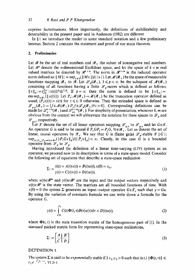
Let ~ be the set of real numbers and ~+ the subset of nonnegative real numbers. Let ~" denote the n-dimensional Euclidean space, and let the space of k x m real valued matrices be denoted by ~k ×,,. The norm in ~k × m is the induced operator norm defined as: II M[I: = s upx,,0(ll Mx II)All x ll ). Let J / ( ~ + ) be the space of measurable functions mapping ~+ to ~. Let ~p(~+) , 1 ~< p < oo be the subspace of . / / (~+) consisting of all functions having a finite ~p-norm which is defined as follows: Ilxll~,:=(~ollx(t)ll~'dt I/p. If p = o o then the norm is defined to be Ilxll~'= ess sup~+ (11 x(t)II ). Let P,:. / /(~+ ) - - . . / / (~ + ) be the truncation operator defined as usual; (Ptx)(z)= x(z) for z ~< t; 0 otherwise. Then the extended space is defined as ~p.~(~+): = { fe . / / (~+) :P , f eL~p(~+)¥ t > 0}. Corresponding definitions can be made for ~ × m ( ~ + ) and k×m ~p.~ (~ + ). For simplicity of presentation, whenever k, m are obvious from the context we will abbreviate the notation for these spaces to ~ p and ~p.~, respectively.

Let ~ denote the set of all linear operators mapping ~'p,e to ~q°p. e and let G~X. An operator G is said to be causal if P~GP t =PtG, Vte~+. Let us denote the set of linear, causal operators by 5f¢. We say that G is (finite gain) ~p-stable if II a I1: sup~e~,..p,x,,0,t~+(ll P, Gx II~)/(ll Ptx I[~) < o~. Clearly, in this case G is a bounded operator from L~ to ~ .

Having introduced the definition of a linear time-varying (LTV) system as an operator, we proceed now to its description in terms of a state-space model. Consider the following set of equations that describe a state-space realization

Yc(t) = A( t )x ( t ) + B(t)u(t) , x(O) = Xo,

y(t) = C(t)x(t) + D(t)u(t), (1)

where u ( t ) ~ m and y ( t ) e~ p are the input and the output vectors respectively and x(t)e~t" is the state vector. The matrices are all bounded functions of time. With x(0) = 0 the system E generates an input-output operator G~X c such that y = Gu. By using the variation of constants formula we can write down a formula for the operator G,

;o y(t) = C(t)~(t, z)B(z)u(r)dz + D(t)u(t), (2)

where ~ ( t , r ) is the state transition matrix of the homogeneous part of (1). In the standard packed matrix form for representing state-space realizations,

DEFINITION 1.

The system E is said to be exponentially stable if 3 cl ,¢2 ~" 0 such that (s.t.) [I O(t, z)11 cle -c2(t-r~, Vt >~ z.

Stability in linear time-varyin9 systems 33

DEFINITION 2.

The system 2 is said to be stabilizable (respectively detectable) if there exists a bounded function K(t) (respectively L(t)) such that system 2(t) = (A - BK)( t )x( t ) (respectively 2(0 = (A - LC)(t)x(t)) is exponentially stable.

It is our intent here to show that the finite gain stability is equivalent to exponential stability for stabilizable and detectable systems.

We end this section with a few results that will be needed in the proof of our main result.

Lemma 2.1. (Desoer & Vidyasagar 1975, p. 115) Let G~Xc. Then G is .~q2p-stable for each 1 <<, p <~ ~ iff G is ~ l-stable and Sly-s table .

Lemma 2.2. Let G ~ X c be the input-output operator correspondin 9 to the system Z as in (1). Let A, B, C, D be bounded functions of time. I f Y, is exponentially stable then G is ~_-w 1 -stable and 5 f ~-stable.

Proof. Easy to derive from the definition of exponential stability.

Lemma 2.3. (Brockett 1970, p. 193) Let ~(t , r ) be the state transition matrix of the system Z with A e S f ~. Then if 3 T > 0 s.t.

iitD(to + T, to)] I 1 ~< ~-Vto~+,

the system is exponentially stable.

3. Main result

Theorem 3.1. Let GE X c be the input-output operator correspondin9 to the system Z

2(0 = A(t)x(t) + B(t)u(t),

y(t) = C(t)x(t) + D(t)u(t). (4)

Let Z be stabilizable and detectable and let 1 <<, p <~ ~ . Then

(1) G is Lfp-stable,

(2) Y~ is exponentially stable.

Proof. (2)=~(t). Follows directly from 1emma (2.1) and lemma (2.2). (1)~(2).

From the definition of stabilizability there exists a bounded function K such that ( A - BK) describes an exponentially stable system. Define v: = u + Kx . Then (4) becomes

2 = A~x + Bv,

y = C ~ x + Dv,

u = v -- Kx , (5)

34 R Ravi and P P Khargonekar

where A l : = (A - B K ) and C1:= ( C - DK). Let T~v denote the operator from v to x. As A 1 is internally stable we have, from lemma (2.2), that T~v is bounded. If Ol(t,z) is the state transition matrix of the system :~ = A ~ x we have

x(t) = ~ l (t, r)B(r)v(~)dr, e f'

y(t) = C, (t)~P l (t, r )B(z)v(r )dz + D(t)v(t),

o

f, u(t) = v(t) - K( t )Ol ( t , z )B(z )v ( z )dr . (6) t o

This means

y = Nv, u = Mv, (7)

where N and M have a state-space realization EN and GM given by

LG I OA' ~ " - [ - ~ J (8)

From the hypothesis, if MvELP; then Nv~LPp. Now let us define two systems X and Y in terms of their realizations Ex and E r as

K K 7 (9)

From the assumption of detectability there is an L such that A - LC is exponentially stable hence both X and Y are exponentially stable. By using simple algebra we can show that

X N + Y M = I. (10)

Multiplying by M-1 on the right,

X N M -1 + Y = M -1

II M-1 II <~ I1 s JI }1G II + II Y II

:~llvllp~<(llXll I/Gtl + 1I YlI)Ilullp (from (7))

II x II p ~< !1 T I1(11S II II G II + II Y II)tl u lip (from (5)).

Set ~ : = II T~olI(IIXII Ilall + II Eli), Consider now the system £1 described below

= A x + u,

y = x , (11)

and let G~ denote the corresponding input-output operator. Clearly E is exponentially stable iff E1 is exponentially stable. We now define a new system that is equivalent to G1 in the input-output sense.

f~l -~- (A - B K ) x l + u, (12)

Stability in linear time-varying systems 35

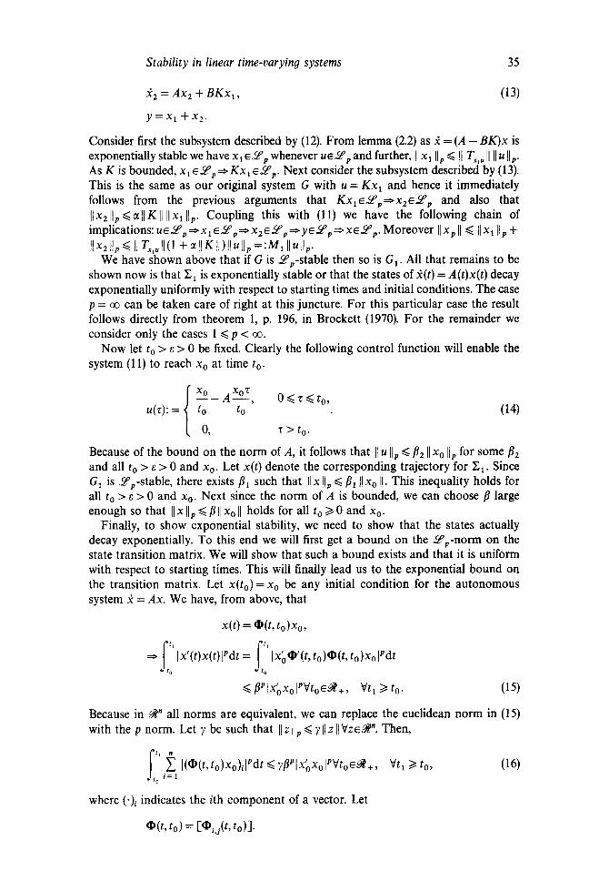
fc 2 = A x 2 + B K x l , (13)

y = x , "+ X 2 .

Consider first the subsystem described by (12). From lemma (2.2) as Y¢ = (A - BK)x is exponentially stable we have x, eZ, ep whenever U~p and further, II x , lip ~< II Tx, u II II u lip. As K is bounded, x , ~ p =~Kx~ e.~p. Next consider the subsystem described by (13). This is the same as our original system G with u = K x , and hence it immediately follows from the previous arguments that K x l e . ~ p ~ x 2 e ~ p and also that IIx211p<<.~Jlgllllx, llp. Coupling this with (11) we have the following chain of implications: U~p=~x,E..,.q~p=>x2e.,q~p:=>yf.~,~'p=>xE.~'p. Moreover Ilxpll ~< IIx~ lip + ]Ix2 Hp ~ < I1Z.,~ 1t(1 +~l]gt l )]]u] lp=:Mx ]lultp.

We have shown above that if G is ~p-stable then so is G~. All that remains to be shown now is that £ , is exponentially stable or that the states of ~(t) = A(t)x(t) decay exponentially uniformly with respect to starting times and initial conditions. The case p = oo can be taken care of right at this juncture. For this particular case the result follows directly from theorem 1, p. 196, in Brockett (1970). For the remainder we consider only the cases 1 ~< p < oo.

Now let to > e > 0 be fixed. Clearly the following control function will enable the system (11) to reach x0 at time to.

x O _ A X ° Z 0~<z~<to ' u(z): = to to (14)

0, z > t o.

Because of the bound on the norm of A, it follows that II u lip ~</~2 II Xo lip for some f12 and all to > e > 0 and Xo. Let x(t) denote the corresponding trajectory for Yq. Since G1 is ~p-stable, there exists fll such that I1 x tip ~</7, II xo ll- This inequality holds for all to > e > 0 and x o. Next since the norm of A is bounded, we can choose fl large enough so that II x lip ~/~ II Xo II holds for all to >/0 and Xo.

Finally, to show exponential stability, we need to show that the states actually decay exponentially. To this end we will first get a bound on the .~qp-norm on the state transition matrix. We will show that such a bound exists and that it is uniform with respect to starting times. This will finally lead us to the exponential bound on the transition matrix. Let X(to)= Xo be any initial condition for the autonomous system £ = Ax. We have, from above, that

x(t) = ~(t , to)Xo,

~ Ix'(t)x(t)lPdt = Ix'o~'(t, to)~(t , to)xolPdt

<, flPlXoXolPVtoe~t +, Mr1 >i to. (15)

Because in ,~n all norms are equivalent, we can replace the euclidean norm in (15) with the p norm. Let y be such that II z ilp ~< '/II z IIVze~". Then,

f " ~ I(~(t, to)Xo),lPdt <~ Vt, >1 (16) yf lPlXoXolPVto~ + , to, i = ,

o

where (')i indicates the ith component of a vector. Let

• (t, to) = [ % / t , to)].

36 R Ravi and P P Khargonekar

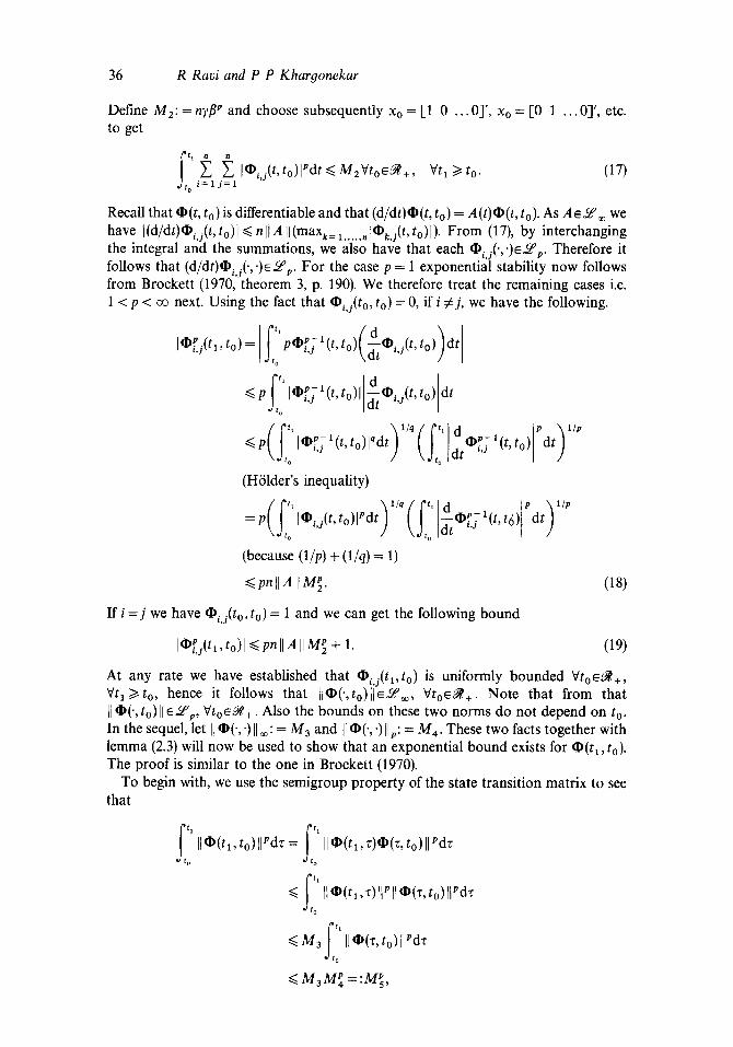
Define M2: =n?fl p and choose subsequently x o = [1 0 . . .0] ' , Xo = [0 1 . . .0] ' , etc. to get

f/ l ~ ~ [*i,J (t'tollpdt<~M2¥to~yl+' Vtl >>'to" (17) o i = l j = l

Recall that ~(t , to) is differentiable and that (d/dt)~(t, to) = A(t)~(t, to). As A e ~ ® we have I(d/dt)~i,j(t, to)l <<. n I1 a II (maxk= 1 ...... r~k,j(t, to)l). From (17), by interchanging the integral and the summations, we also have that each ~i.j(',')~Lep" Therefore it follows that (d/dt)~i,j(., ")e~p. For the case p = 1 exponential stability now follows from Brockett (1970, theorem 3, p. 190). We therefore treat the remaining cases i.e. 1 < p < oo next. Using the fact that ~i.j(to, to) = 0, if i ~ j , we have the following.

I*~,j(t~,to)= f/o' p*~.f ~(t, to)( d ",.~(t, to))dt

<~ p f/o~l~PPf ~(t, to)l dtoP,,j(t, to) dt

<~p I*~,f'(t, to)lqdt) ( | *~,f'(t, • 2 t o / \ q¢ t o

(H61der's inequality)

d _¢pe- (t, t6) dt) =P(f/o'lO'd(t't°)lPdt)'/q(fto ' d t L J 1 P X ~ l / P

(because (I/p) + (l/q) = 1)

<~ pn II AII M~. (18)

If i = j we have ~ij(to, to) = 1 and we can get the following bound

[lll~,j(tl, to)l ~< pn II A II M~ + 1. (19)

At any rate we have established that ~.i(t~,to) is uniformly bounded V t o ~ + , Vta>~to, hence it follows that II~(',to)ll~LP~, V t o ~ ÷ . Note that from that II~(', to)II ~ p , V t o ~ + . Also the bounds on these two norms do not depend on to. In the sequel, let II ~( ' , ')II ® := M3 and II ~(',')I1~: = M4. These two facts together with lemma (2.3) will now be used to show that an exponential bound exists for ~ ( t l , to). The proof is similar to the one in Brockett (1970).

To begin with, we use the semigroup property of the state transition matrix to see that

~ 'o' II O(q , to)llPdv =

~<

~<

~<

f " ii~(q,v)~(~,to)llPdv to

f '~ IL*(tl, 3)IL ~ 11"(3, to)IVdz o

M3 II ~(3, to)HPd3 o

M 3 M~ = :M~,

Stability in linear time-varyin 9 systems 37

from which it follows that

(t 1 - to)l/Pll®(tl , to)[l <~ M 5.

Now define T: = (2M5) v to get

1 I]~(to+ T, t0)[[ ~< .

2

The conclusion that G is exponentially stable now follows straight from lemma (2.3). •

This work was supported in part by the National Science Foundation under grant ECS-8451519, in part by a grant from GE, and in part by US Air Force Office of Scientific Research under grant AFOSR-88-0020. The first author was also supported by a University of Minnesota Graduate Dissertation Fellowship.

References

Anderson B D O 1982 Internal and external stability of linear time-varying systems. SIAM J Control Optimization 20:408-413

Brockett R W 1970 Finite dimensional linear systems (New York: John Wiley) Desoer C A, Vidyasagar M 1975 Feedback systems: Input-output properties (New York:

Academic Press) Ravi R, Khargonekar P P 1989 On the equivalence between exponential stability and input-

output stability for linear time-varying continuous-time systems, Tech. Report, Department of Electrical Engineering, University of Minnesota, Minneapolis, September