Embed Size (px)
Citation preview
Exploring Scatterer Anisotropyin Synthetic Aperture Radarvia Sub-aperture Analysis
by
Andrew J. Kim
B.E.E., Georgia Institute of Technology, 1995S.M.E.E., Massachusetts Institute of Technology, 1997
Submitted to the Department of Electrical Engineering and Computer Sciencein partial fulfillment of the requirements for the degree of
Doctor of Philosophyin Electrical Engineering and Computer Scienceat the Massachusetts Institute of Technology
September 2001
c© 2001 Massachusetts Institute of TechnologyAll Rights Reserved.

2
Exploring Scatterer Anisotropyin Synthetic Aperture Radarvia Sub-aperture Analysis
by Andrew J. Kim
Submitted to the Department of Electrical Engineering and Computer Scienceon August 31, 2001 in Partial Fulfillment of the Requirements
for the Degree of Doctor of Philosophyin Electrical Engineering and Computer Science
Abstract
Scattering from man-made objects in SAR imagery exhibits aspect and frequencydependencies which are not always well modeled by standard SAR imaging techniquesbased on the ideal point scattering model. This is particularly the case for high-resolution wide-band and wide-aperture data where model deviations are even morepronounced. If ignored, these deviations will reduce recognition performance due tothe model mismatch, but when appropriately accounted for, these deviations from theideal point scattering model can be exploited as attributes to better distinguish scat-terers and their respective targets. With this in mind, this thesis develops an efficientmodeling framework based on a sub-aperture pyramid to utilize scatterer anisotropy forthe purpose of target classification. Two approaches are presented to exploit scattereranisotropy using the sub-aperture pyramid. The first is a nonparametric classifier thatlearns the azimuthal dependencies within an image and makes a classification decisionbased on the learned dependencies. The second approach is a parametric attributionof the observed anisotropy characterizing the azimuthal location and concentration ofthe scattering response. Working from the sub-aperture scattering model, we developa hypothesis test to characterize anisotropy. We start with an isolated scatterer modelwhich produces a test with an intuitive interpretation. We then address the problem ofrobustness to interfering scatterers by extending the model to account for neighboringscatterers which corrupt the anisotropy attribution. The development of the anisotropyattribution culminates with an iterative attribution approach that identifies and com-pensates for neighboring scatterers. In the course of the development of the anisotropyattribution, we also study the relationship between scatterer phenomenology and ouranisotropy attribution. This analysis reveals the information provided by the anisotropyattribution for two common sources of anisotropy. Furthermore, the analysis explicitlydemonstrates the benefit of using wide-aperture data to produce more stable and moredescriptive characterizations of scatterer anisotropy.
Thesis Supervisor: Alan S. WillskyTitle: Edwin S. Webster Professor of Electrical Engineering

4
Acknowledgments
First and foremost, I thank my advisor Alan Willsky. Any words that I use will lackthe eloquence to convey how deeply I appreciate Alan’s help over the past six years.His guidance and support have significantly helped me mature as a researcher. Notonly has he helped my research with his vast technical insight, but he has also helpedme to define, analyze, and explain to others the underlying problems that need to beaddressed.
I would also like to thank the members of my thesis committee: John Fisher, JeffShapiro, and Paul Viola. Their comments and assistance have also significantly con-tributed to my research. Particular thanks must be made to John Fisher. I have hadthe great opportunity to interact with John who has served as both a member of mycommittee and a research scientist in Alan’s group. With his ideas and contributions,John has been like a second advisor to me. John has also been a great friend, Orlandotour guide, and football pool participant.
Throughout my years in college, my life has been influenced by many people. Iconsider myself most fortunate to have made such friends. Walter Sun has a strengthof character in him that I have never seen in anyone else. Our friendship started while wewere undergraduates and continues to be strong even though separated by thousands ofmiles these past few years. Every season, I can look forward to disagreeing with Walteron the relative strength of collegiate teams in various sports. Dewey Tucker is anothergreat friend that I have had the pleasure of knowing since our days at Georgia Tech.Though I tease Dewey a lot for “following me to MIT and the SSG lab1”, I am glad heis around. Dewey is a great friend with whom I have had great times and been able totalk to during difficult times.
Besides Dewey Tucker and John Fisher, there are a number of great people in theSSG lab that I have enjoyed being around these past six years. John Richards hasbeen a great friend, fellow SAR grouplet member, officemate, classmate, SPIE travelcompanion, and football pool participant. John could always be counted on for hisposting of highlights from “The Onion”, jokes about Canadians, and Big-10 sports bias.Alex Ihler and I have shared many interests. I most thank Alex for getting me involvedin Shotokan Karate. I will miss our discussions and shared efforts in administering the
1He will probably also “follow” me back to Atlanta.
5
6
SSG computer network, “examining video compression formats”, and anime. CedricLogan is the founding father of the “manifesto board” and fellow SAR grouplet member.I will miss our (John R.’s, Cedric’s, and my) regular trips to the food trucks (I’ll missour trips and discussions – not the food). Conversations with fellow officemate MikeSchneider will also be missed. Mike could always be counted on to provide a stimulatingdiscussion on technical trends, software copyrights, social issues, and many other topics.Being the lone Canadian in the group, Martin Wainwright has amicably served as theobject of all of our Canadian jokes (but it is not as if he had a choice). And, despitehis disparaging comments of American society, we recognize that those comments areonly out of envy. Taylore Kelly serves as the keystone holding the group together. Thegroup could not function as smoothly without her support and would not be as much funwithout her humor. In addition to these people, I would also like to thank other groupmembers Mike Daniel, Seema Jaggi, Rachel Learned, Terrance Ho, Charlie Fosgate,Ilya Pollak, Austin Frakt, Andy Tsai, Junmo Kim, Erik Sudderth, Jason Johnson,Mujdat Cetin, Ben Halpern, Gerald Spica, and Paula Place-Cordiero for their help andfriendship throughout the years.
I would also like to recognize members of the MIT SKA dojo. My only regret intaking karate is not having started earlier. The rewards of the physical and mentalconditioning cannot be put into words, but a person needs only to see the intenseefforts that students put into their training to understand that these rewards must besomething special. Dojo instructor Johnson Chung taught me physical technique, mind-set, and self-discipline. In addition to being a wonderful teacher during the practice, heis a great friend outside of practice. Club captain Alex Ihler introduced me to karateand is always willing to answer any question I have throughout the day. My seniors havealso helped with my training and served as good friends. These are: Jesse Winch, EstiKassovicz, Renata Gebauer, Elizabeth Fong, Kang Liu, Edem Tsikata, Ben Holland,Jeff Miller, Tolulope Okusanya, and Pablo Serafini.
Three other close friends at MIT deserve mention. Nick Laneman and EdmundYeh, who I met my first week at MIT, have been through a lot with me from classesand doctoral qualifying exams to regular (and then irregular) lunch meetings. GaryCheng, my first year roommate and fellow PAC-10 fan, has endure the east-coast biasthat prevails not only the everyday people here but also the local press. I can alwayscount on Gary to inform me of when UCLA accomplishes something worthwhile.
I am infinitely indebted to my parents Chang and Theresa Kim and my siblings JoeKim, Cecilia Kim, Tina Engle, and Patrick Kim. They have been a source of supportand advice not just through my graduate studies but throughout my life. Without theirhelp, I would not have been able to persevere through many difficult times and attainwhat I have in life.
Contents
Abstract 3
Acknowledgments 5
List of Figures 11
List of Tables 19
Notational Conventions 21Mathematical Notation . . . . . . . . . . . . . . . . . . . . . . . . . . . . . . 21Commonly Used Variables . . . . . . . . . . . . . . . . . . . . . . . . . . . . . 21Common Acronyms . . . . . . . . . . . . . . . . . . . . . . . . . . . . . . . . 22
1 Introduction 231.1 Premise . . . . . . . . . . . . . . . . . . . . . . . . . . . . . . . . . . . . 251.2 Previous Efforts . . . . . . . . . . . . . . . . . . . . . . . . . . . . . . . . 251.3 Thesis Objective . . . . . . . . . . . . . . . . . . . . . . . . . . . . . . . 281.4 Thesis Organization . . . . . . . . . . . . . . . . . . . . . . . . . . . . . 30
1.4.1 Background . . . . . . . . . . . . . . . . . . . . . . . . . . . . . . 301.4.2 Sub-aperture Analysis . . . . . . . . . . . . . . . . . . . . . . . . 301.4.3 Nonparametric Estimation of Anisotropy . . . . . . . . . . . . . 301.4.4 Sub-aperture Anisotropy Attribution . . . . . . . . . . . . . . . . 311.4.5 Anisotropy Phenomenology . . . . . . . . . . . . . . . . . . . . . 311.4.6 Iterative Anisotropy Attribution . . . . . . . . . . . . . . . . . . 321.4.7 Conclusions . . . . . . . . . . . . . . . . . . . . . . . . . . . . . . 32
2 Background 332.1 Conventional SAR . . . . . . . . . . . . . . . . . . . . . . . . . . . . . . 33
2.1.1 Matched Filter Range Compression . . . . . . . . . . . . . . . . . 362.1.2 Matched Filter Cross-Range Compression . . . . . . . . . . . . . 372.1.3 Deramp Pulse Compression . . . . . . . . . . . . . . . . . . . . . 40
2.2 Spectral Estimation and SAR . . . . . . . . . . . . . . . . . . . . . . . . 43
7
8 CONTENTS
2.2.1 Conventional Beamformer . . . . . . . . . . . . . . . . . . . . . . 462.2.2 Capon’s Beamformer . . . . . . . . . . . . . . . . . . . . . . . . . 46
2.3 Nonideal Scattering . . . . . . . . . . . . . . . . . . . . . . . . . . . . . . 472.4 Machine Learning . . . . . . . . . . . . . . . . . . . . . . . . . . . . . . . 52
2.4.1 Kernel Based Density Estimation . . . . . . . . . . . . . . . . . . 522.4.2 Information and Entropy . . . . . . . . . . . . . . . . . . . . . . 542.4.3 KL-Based Classification Technique . . . . . . . . . . . . . . . . . 55
3 Sub-aperture Representation 593.1 Sub-aperture Pyramid . . . . . . . . . . . . . . . . . . . . . . . . . . . . 613.2 Sub-aperture Reflectivity . . . . . . . . . . . . . . . . . . . . . . . . . . 623.3 Interpretations . . . . . . . . . . . . . . . . . . . . . . . . . . . . . . . . 65
3.3.1 Time-Frequency Plane Tilings . . . . . . . . . . . . . . . . . . . . 653.3.2 Matched Filter Bank . . . . . . . . . . . . . . . . . . . . . . . . . 67
4 Nonparametric Estimation of Anisotropy 694.1 Problem Setting . . . . . . . . . . . . . . . . . . . . . . . . . . . . . . . 704.2 Nonparametric Sub-aperture Based Classifier . . . . . . . . . . . . . . . 70
4.2.1 Sub-aperture Feature Vector . . . . . . . . . . . . . . . . . . . . 704.2.2 Density Estimation . . . . . . . . . . . . . . . . . . . . . . . . . . 724.2.3 Density Comparison . . . . . . . . . . . . . . . . . . . . . . . . . 734.2.4 Feature Space Discretization . . . . . . . . . . . . . . . . . . . . 744.2.5 Kernel Width Selection . . . . . . . . . . . . . . . . . . . . . . . 77
4.3 Experimental Results . . . . . . . . . . . . . . . . . . . . . . . . . . . . . 784.3.1 Kernel Width . . . . . . . . . . . . . . . . . . . . . . . . . . . . . 784.3.2 ROC curves . . . . . . . . . . . . . . . . . . . . . . . . . . . . . . 80
5 Sub-aperture Anisotropy Attribution 855.1 Anisotropy Attribution – Isolated Scatterer Model . . . . . . . . . . . . 86
5.1.1 Observation Model . . . . . . . . . . . . . . . . . . . . . . . . . . 865.1.2 Hypothesis Test Example . . . . . . . . . . . . . . . . . . . . . . 885.1.3 GLLR . . . . . . . . . . . . . . . . . . . . . . . . . . . . . . . . . 905.1.4 Comparison to Chaney and Allen . . . . . . . . . . . . . . . . . . 945.1.5 Modified GLLR . . . . . . . . . . . . . . . . . . . . . . . . . . . . 965.1.6 Sub-aperture Scattering Model Deviations . . . . . . . . . . . . . 975.1.7 Experimental Results . . . . . . . . . . . . . . . . . . . . . . . . 98
5.2 Anisotropy Attribution – Multiple Scatterer Model . . . . . . . . . . . . 1025.2.1 Model and Test . . . . . . . . . . . . . . . . . . . . . . . . . . . . 1025.2.2 Experimental Results . . . . . . . . . . . . . . . . . . . . . . . . 106
5.3 Decision-Directed Telescopic Testing . . . . . . . . . . . . . . . . . . . . 1075.3.1 Telescopic Algorithm . . . . . . . . . . . . . . . . . . . . . . . . . 1085.3.2 Results . . . . . . . . . . . . . . . . . . . . . . . . . . . . . . . . 109
5.4 Results on MSTAR Data . . . . . . . . . . . . . . . . . . . . . . . . . . 110
CONTENTS 9
5.4.1 Images of Anisotropy . . . . . . . . . . . . . . . . . . . . . . . . . 1115.4.2 Confusion Matrices . . . . . . . . . . . . . . . . . . . . . . . . . . 1125.4.3 Summary of MSTAR Results . . . . . . . . . . . . . . . . . . . . 113
6 Relation between Phenomenology and Anisotropy Attribution 1176.1 Geometric Anisotropy . . . . . . . . . . . . . . . . . . . . . . . . . . . . 1196.2 Volumetric Anisotropy . . . . . . . . . . . . . . . . . . . . . . . . . . . . 1246.3 Extensions to Wide-Aperture Data . . . . . . . . . . . . . . . . . . . . . 1266.4 Additional Wide-aperture Hypotheses . . . . . . . . . . . . . . . . . . . 1316.5 Wide-aperture GUS Data . . . . . . . . . . . . . . . . . . . . . . . . . . 134
7 Iterative Anisotropy Attribution 1417.1 Algorithm Overview . . . . . . . . . . . . . . . . . . . . . . . . . . . . . 1427.2 Pixel Aggregation . . . . . . . . . . . . . . . . . . . . . . . . . . . . . . . 145
7.2.1 Problem Setup . . . . . . . . . . . . . . . . . . . . . . . . . . . . 1457.2.2 Aggregation Likelihood . . . . . . . . . . . . . . . . . . . . . . . 1467.2.3 Greedy Aggregation Algorithm . . . . . . . . . . . . . . . . . . . 1487.2.4 Aggregation Results . . . . . . . . . . . . . . . . . . . . . . . . . 149
7.3 Anisotropy Re-attribution . . . . . . . . . . . . . . . . . . . . . . . . . . 1527.3.1 Re-attribution Algorithm . . . . . . . . . . . . . . . . . . . . . . 1537.3.2 Comments about the Algorithm . . . . . . . . . . . . . . . . . . 157
7.4 Experimental Results . . . . . . . . . . . . . . . . . . . . . . . . . . . . . 159
8 Contributions and Suggestions for Future Research 1758.1 Summary of Contributions . . . . . . . . . . . . . . . . . . . . . . . . . . 1758.2 Suggestions for Future Research . . . . . . . . . . . . . . . . . . . . . . . 179
A DeBonet’s Wavelet-based Classifier 183A.1 Wavelet-based Representation . . . . . . . . . . . . . . . . . . . . . . . . 183A.2 Learning Dependencies . . . . . . . . . . . . . . . . . . . . . . . . . . . . 186A.3 Decision Rule . . . . . . . . . . . . . . . . . . . . . . . . . . . . . . . . . 186
B MSTAR Data Set 189
Bibliography 191

10 CONTENTS
List of Figures
1.1 SAR Imaging scenario. . . . . . . . . . . . . . . . . . . . . . . . . . . . 24
2.1 Terminology used in SAR imaging. . . . . . . . . . . . . . . . . . . . . 342.2 Illustration of the imaging planes (shaded region) for (a) SAR and (b)
photographical imagery. . . . . . . . . . . . . . . . . . . . . . . . . . . . 352.3 Multiple cross-range sensor measurements of the target field. . . . . . . 382.4 Mixing the received signal with a delayed extended chirp. . . . . . . . . 412.5 Mixing signals to produce a sinusoid whose frequency is proportional to
the distance from the center of the footprint. . . . . . . . . . . . . . . . 422.6 Illustration of the array processing scenario for a uniform linear array.
(a) Far-field source and incident plane waves. (b) Antenna pattern for agiven set of sensor weights. . . . . . . . . . . . . . . . . . . . . . . . . . 44
2.7 Illustrations of canonical scatterers. . . . . . . . . . . . . . . . . . . . . 492.8 Azimuthal responses for canonical scatterers from the PO model. . . . 502.9 Example of Parzen density estimation. . . . . . . . . . . . . . . . . . . 53
3.1 Illustration of a sub-aperture pyramid. . . . . . . . . . . . . . . . . . . 593.2 Illustration of how different azimuthal responses (bottom) are repre-
sented on the sub-aperture pyramid (top). . . . . . . . . . . . . . . . . 603.3 Three examples of sub-aperture pyramids. (a) Disjoint, half-aperture
pyramid. (b) Half-overlapping, half-aperture pyramid. (c) Eighth-incrementing,half-aperture pyramid. . . . . . . . . . . . . . . . . . . . . . . . . . . . 62
3.4 The response of a 1m× 1m flat plate and a depiction of the reflectivityestimate for each of the sub-apertures. Lighter shaded sub-aperturesconvey larger reflectivity estimates. . . . . . . . . . . . . . . . . . . . . 64
11
12 LIST OF FIGURES
3.5 Left: Disjoint, half-aperture pyramid. Right: Corresponding sub-apertureimages of a BMP-2 at a 17◦ elevation and 0◦ azimuth. For each image,the front of the vehicle is the portion nearest the left edge of the image.The azimuthal flash due to the front of the tank can be seen from thequarter-aperture images to be predominantly contained in the middlesection of the aperture. However, while providing more azimuthal in-formation about the scattering, these smaller sub-aperture images sufferfrom severe sidelobe artifacts as can be seen from the front plate responsecorrupting the reflectivity estimates in neighboring cross-range pixels. . 64
3.6 Tilings of the azimuth–cross-range plane. (a) Full-aperture tiling. (b)Half-aperture tiling. (c) Quarter-aperture tiling. . . . . . . . . . . . . . 66
3.7 Tilings of the azimuth–cross-range plane and how they represent a dis-tributed scatterer. (a) The underlying scatterer’s energy coverage inazimuth and cross-range. (b) Full-aperture representation. (c) Half-aperture representation. (d) Quarter-aperture representation. . . . . . 67
3.8 (a) Wavelet tiling of the azimuth–cross-range plane. (b) A level of a“pyramid” which would produce such a tiling. . . . . . . . . . . . . . . 67
4.1 The dyadic tree structure for pixels that results from using a half-aperturesplitting scheme in the sub-aperture pyramid. The feature vector for theshaded pixel is indicated by the shaded branch. . . . . . . . . . . . . . 71
4.2 The relationship between (left) the half-overlapping, half-aperture sub-aperture pyramid and (right) the corresponding feature vector tree. . . 72
4.3 Flow diagram illustrating the clustering procedure used to generate auniform sampling over the union of the supports of the reference densities. 75
4.4 Two densities used to illustrate the difference in emphasis between tra-ditional density estimation and density estimation for the purpose ofdiscrimination. . . . . . . . . . . . . . . . . . . . . . . . . . . . . . . . . 78
4.5 Flow diagram illustrating the kernel width selection procedure. . . . . . 794.6 Coordinate descent optimization of the kernel width using the KLD rule
in Eq. (4.3). (a) Optimizing over the coarsest scale h(2) with h(0) = 5.3and h(1) = 2.6. (b) Optimizing over h(1) with h(0) = 5.3 and h(2) = 17.4.(c) Optimizing over the finest scale h(0) with h(1) = 2.6 and h(2) = 17.4. 80
4.7 Coordinate descent optimization of the kernel width using the χ2 rule inEq. (4.4). (a) Optimizing over the coarsest scale h(2) with h(0) = 15.0 andh(1) = 14.6. (b) Optimizing over h(1) with h(0) = 15.0 and h(2) = 17.2.(c) Optimizing over the finest scale h(0) with h(1) = 14.6 and h(2) = 17.2. 80
4.8 ROC detection curves for the (a) BMP-2, (b) BTR-70, and (c) T-72using the KLD rule with hKL (solid curve), the χ2 rule with hχ2 (dashedcurve), and the KLD rule with with hχ2 (dashed-dotted curve). . . . . 82
LIST OF FIGURES 13
4.9 ROC detection curves for the (a) BMP-2, (b) BTR-70, and (c) T-72 usingthe χ2 rule with hχ2 (solid curve), DeBonet’s algorithm (dashed curve),and the WPAFB template matching algorithm (dashed-dotted curve). . 83
5.1 Illustration of how an interfering scatterer can cause a false anisotropyclassification with the GLLR in Eq. (5.16). . . . . . . . . . . . . . . . . 96
5.2 Log-magnitude image of the SAR data used to examine the anisotropyattribution methods. (a) Image without scatterer labels. (b) Image withtrue scatterer labels. . . . . . . . . . . . . . . . . . . . . . . . . . . . . 99
5.3 Results of using: (a,b) the reflectivity statistic; (c,d) the basic GLLR; and(e,f) the modified GLLR on the SAR data in Figure 5.2. Left column:images of degree of anisotropy. Right column: images of sub-aperturereflectivity. . . . . . . . . . . . . . . . . . . . . . . . . . . . . . . . . . . 101
5.4 Results of using a pre-screening threshold with: (a,b) the reflectivitystatistic; (c,d) the basic GLLR; and (e,f) the modified GLLR on theSAR data in Figure 5.2. Left column: images of degree of anisotropy.Right column: images of sub-aperture reflectivity. . . . . . . . . . . . . 103
5.5 Results of using the anisotropy test based on the MSM statistic appliedto the SAR data in Figure 5.2. Images of (a) degree of anisotropy and(b) sub-aperture reflectivity. . . . . . . . . . . . . . . . . . . . . . . . . 107
5.6 Results of using the anisotropy test based on the MSM statistic with apre-screening threshold applied to the SAR data in Figure 5.2. Imagesof (a) degree of anisotropy and (b) sub-aperture reflectivity. . . . . . . 107
5.7 Illustration of how the anisotropy testing can be done in a decision-directed fashion by starting with the full-aperture, and at each scale,inspecting only the children of the most likely sub-aperture. The test-ing terminates as soon as the parent is sufficiently more likely than itschildren or the bottom of the pyramid is reached. Lighter shadings ofthe sub-apertures indicate higher likelihoods. Dashed lines denote whichhypotheses are tested, and solid lines denote the branch traversed. . . . 109
5.8 Results of using the telescopic testing procedure (a-b) with the modi-fied GLLR and (c-d) with the MSM statistic. Images of (a,c) degree ofanisotropy and (b,d) sub-aperture reflectivity. . . . . . . . . . . . . . . 110
5.9 Results of using the telescopic testing procedure and a pre-screeningthreshold (a-b) with the modified GLLR and (c-d) with the MSM statis-tic. Images of (a,c) degree of anisotropy and (b,d) sub-aperture reflec-tivity. . . . . . . . . . . . . . . . . . . . . . . . . . . . . . . . . . . . . . 111
5.10 Anisotropy characterization of a BMP-2 at (first row) 0◦ azimuth, (sec-ond row) 30◦ azimuth, (third row) 60◦ azimuth, and (fourth row) 90◦
azimuth. First column: Images of log-magnitude reflectivities. Middlecolumn: Image of anisotropy classifications. Last column: Image of sub-aperture reflectivities. . . . . . . . . . . . . . . . . . . . . . . . . . . . . 115
14 LIST OF FIGURES
6.1 Instances of azimuthal scattering by a (a) geometric scatterer and (b)volumetric scatterer with the real and imaginary components of the re-sponse shown in the solid and dashed lines respectively. . . . . . . . . . 118
6.2 Anisotropy plots for a square plate in Gaussian noise at 20dB PSNR and(a) no azimuthal and location uncertainty; (b) maximal azimuthal uncer-tainty and no location uncertainty; (c) maximal azimuthal uncertaintyand location uncertainty given by peak extraction. . . . . . . . . . . . . 120
6.3 Azimuthal response for different plate sizes: (a) 0.9m, (b) 1.6m, and (c)2.6m. . . . . . . . . . . . . . . . . . . . . . . . . . . . . . . . . . . . . . 121
6.4 Anisotropy plots for volumetric scatterers with a scattering density of(a) 1, (b) 10, and (c) 100 scatterers per resolution cell. . . . . . . . . . 126
6.5 Anisotropy plots based on wide-aperture data for the canonical flat platescatterer using (a) the coarse-resolution peak extraction and (b) the fine-resolution peak extraction. . . . . . . . . . . . . . . . . . . . . . . . . . 129
6.6 Anisotropy plots based on wide-aperture data for volumetric scattererswith scattering density of 10 scatterers per coarse-resolution cell using(a) the coarse-resolution peak extraction and (b) the fine-resolution peakextraction. . . . . . . . . . . . . . . . . . . . . . . . . . . . . . . . . . . 130
6.7 Anisotropy plots using the hybrid-resolution peak extraction for (a) thecanonical flat plate scatterer and (b) the volumetric scatterer with 10scatterers per coarse resolution cell. . . . . . . . . . . . . . . . . . . . . 131
6.8 Anisotropy plots for the canonical flat plate scatterer using the aug-mented hypothesis set and (a) the coarse-resolution peak extraction, (b)the fine-resolution peak extraction, and (c) the hybrid-resolution peakextraction. . . . . . . . . . . . . . . . . . . . . . . . . . . . . . . . . . . 132
6.9 Anisotropy plots for volumetric scatterers with a scattering density of10 scatterers per coarse resolution cell using the augmented hypothesisset and (a) the coarse-resolution peak extraction, (b) the fine-resolutionpeak extraction, and (c) the hybrid-resolution peak extraction. . . . . . 133
6.10 Anisotropy characterization of peaks from wide-aperture data for vehicle1. (a) Narrow-aperture log-magnitude image. (b) Narrow-aperture imagewith anisotropy overlays. (c) Wide-aperture log-magnitude image. (d)Wide-aperture image with anisotropy overlays. . . . . . . . . . . . . . . 135
6.11 Anisotropy characterization of peaks from wide-aperture data for vehicle2. (a) Narrow-aperture log-magnitude image. (b) Narrow-aperture imagewith anisotropy overlays. (c) Wide-aperture log-magnitude image. (d)Wide-aperture image with anisotropy overlays. . . . . . . . . . . . . . . 136
6.12 Anisotropy characterization of peaks from 3 instances of clutter in theGUS data. Left: Narrow-aperture anisotropy attributions. Right: Wide-aperture anisotropy attributions. . . . . . . . . . . . . . . . . . . . . . . 138
7.1 The iterative attribution algorithm used to classify anisotropy. . . . . . 143
LIST OF FIGURES 15
7.2 Standard log-magnitude image of the synthesized SAR data used inChapter 5 (a) without annotations and (b) with annotations describ-ing the individual scatterers. A circle denotes an isotropic scatterer; asquare denotes a half-aperture scatterer; and a triangle denotes a quarter-aperture scatterer. The large ellipses denote which scatterers are used todefine a particular down-range value (i.e. DR1, DR2, DR3, and DR4). . 150
7.3 (a) Reflectivity of all cross-range pixels at down-range DR3 containingthe isotropic scatterer A6 and quarter-aperture scatterer C1. (b) Seg-mentation for pixels at down-range DR3. . . . . . . . . . . . . . . . . . 151
7.4 (a) Reflectivity of all cross-range pixels at down-range DR4 containingthe half-aperture scatterersD1 andD2 and the quarter-aperture scattererC2. (b) Segmentation for pixels at down-range DR4. . . . . . . . . . . 152
7.5 Illustration of reducing the model order of A by removing neighboring,on-scatterer components to produce A. . . . . . . . . . . . . . . . . . . 155
7.6 Illustration of why the reflectivity is incorrectly estimated in the earlystages of the telescopic test on a spatially distributed scatterer. The sincfunction is centered at the scattering center, but the sinc associated withthe hypothesis being tested is too narrow. The point we are trying tofit (labeled with a cross-hatch) corresponds to a sidelobe of the sinc, butthe observation model in Eq. (7.15) assumes that the sinc mainlobe spansthe entire scatterer. Thus, the estimated reflectivity is in gross error andseverely distorts the anisotropy characterization. . . . . . . . . . . . . . 157
7.7 Results of the iterative anisotropy attribution on the synthesized data inFigure 7.2. First column: images of the degree of anisotropy. Second col-umn: images of the resulting sub-aperture reflectivities. First row: initialattribution using the MSM statistic from Chapter 5. Second row: firstanisotropy re-attribution. Third row: second anisotropy re-attribution. 161
7.8 Segmentation of pixels at down-range DR1 in Figure 7.2. (a) Full-aperturereflectivity. (b) Segmentation based on the initial anisotropy attribution.(c) Segmentation based on the first anisotropy re-attribution. (d) Seg-mentation based on the second anisotropy re-attribution. . . . . . . . . 163
7.9 Segmentation of pixels at down-range DR2 in Figure 7.2. (a) Full-aperturereflectivity. (b) Segmentation based on the initial anisotropy attribution.(c) Segmentation based on the first anisotropy re-attribution. (d) Seg-mentation based on the second anisotropy re-attribution. . . . . . . . . 164
7.10 Segmentation of pixels at down-range DR3 in Figure 7.2. (a) Full-aperturereflectivity. (b) Segmentation based on the initial anisotropy attribution.(c) Segmentation based on the first anisotropy re-attribution. (d) Seg-mentation based on the second anisotropy re-attribution. . . . . . . . . 165
16 LIST OF FIGURES
7.11 Segmentation of pixels at down-range DR4 in Figure 7.2. (a) Full-aperturereflectivity. (b) Segmentation based on the initial anisotropy attribution.(c) Segmentation based on the first anisotropy re-attribution. (d) Seg-mentation based on the second anisotropy re-attribution. . . . . . . . . 166
7.12 Log-magnitude image of the SAR data with closely spaced scatterers (a)without annotations and (b) with annotations. . . . . . . . . . . . . . . 167
7.13 Results of the iterative anisotropy attribution on the synthesized datain Figure 7.12. First column: images of the degree of anisotropy. Sec-ond column: images of the resulting sub-aperture reflectivities. Firstrow: initial attribution using the MSM statistic from Chapter 5. Sec-ond row: first anisotropy re-attribution. Third row: second anisotropyre-attribution. . . . . . . . . . . . . . . . . . . . . . . . . . . . . . . . . 168
7.14 Segmentation of pixels at down-range DR2 in Figure 7.12. (a) Full-aperture reflectivity. (b) Segmentation based on the initial anisotropy at-tribution. (c) Segmentation based on the first anisotropy re-attribution.(d) Segmentation based on the second anisotropy re-attribution. . . . . 169
7.15 Segmentation of pixels at down-range DR3 in Figure 7.12. (a) Full-aperture reflectivity. (b) Segmentation based on the initial anisotropy at-tribution. (c) Segmentation based on the first anisotropy re-attribution.(d) Segmentation based on the second anisotropy re-attribution. . . . . 170
7.16 Segmentation of pixels at down-range DR4 in Figure 7.12. (a) Full-aperture reflectivity. (b) Segmentation based on the initial anisotropy at-tribution. (c) Segmentation based on the first anisotropy re-attribution.(d) Segmentation based on the second anisotropy re-attribution. . . . . 171
7.17 Standard full-aperture log-magnitude reflectivity image of a BMP-2 tankat an (a) 0◦ azimuth and (b) 90◦ azimuth. . . . . . . . . . . . . . . . . 172
7.18 Anisotropy attributions and reflectivity images of the BMP-2 at a 0◦
azimuth. First column: images of the anisotropy attributions. Sec-ond column: images of the associated sub-aperture reflectivities. Firstrow: initial anisotropy attribution. Second row: fourth iteration of theanisotropy attribution. . . . . . . . . . . . . . . . . . . . . . . . . . . . 173
7.19 Anisotropy attributions and reflectivity images of the BMP-2 at a 90◦
azimuth. First column: images of the anisotropy attributions. Sec-ond column: images of the associated sub-aperture reflectivities. Firstrow: initial anisotropy attribution. Second row: fourth iteration of theanisotropy attribution. . . . . . . . . . . . . . . . . . . . . . . . . . . . 174
A.1 Generation of the wavelet-based feature vectors. Left-hand side: Con-struction of the multiresolution SAR images Gm. Right-hand side: Fil-tering of multiresolution images to reveal image structure. . . . . . . . 184
LIST OF FIGURES 17
A.2 Illustration a multiresolution feature vector used by DeBonet. Eachvector-valued image is composed of the filtered images for the corre-sponding resolution. Each branch (such as the heavily shaded path) inthe resulting quad-tree constitutes a feature vector. . . . . . . . . . . . 185

18 LIST OF FIGURES

List of Tables
5.1 Cost matrix used to establish thresholds in the GLLR-based decision rules. 995.2 Anisotropy confusion matrix for 2S1, BMP-2, BRDM-2, D7, T-72, ZIL-
131, and ZSU-23/4. . . . . . . . . . . . . . . . . . . . . . . . . . . . . . . 1135.3 Anisotropy confusion matrix for vehicles at near-cardinal and off-cardinal
angles. . . . . . . . . . . . . . . . . . . . . . . . . . . . . . . . . . . . . . 114
6.1 GLLR’s for noiseless 2.6m plate response (assuming an PSNR of 20dB). 1226.2 Anisotropy classification correspondences for clutter with narrow and
wide-aperture data using the same anisotropy hypotheses. . . . . . . . . 1376.3 Anisotropy classification correspondences for clutter with narrow and
wide-aperture data using the augmented hypothesis set for wide-aperturedata. . . . . . . . . . . . . . . . . . . . . . . . . . . . . . . . . . . . . . . 139
19

20 LIST OF TABLES

Notational Conventions
Mathematical Notation
·∗ conjugation, e.g. a∗
· ∗ ·· convolution, e.g. x(t) ∗ y(t)·H hermitian transpose
P−→N→∞
convergence in probability as N tends to infinity
∼ distributed according to·T transpose
‖ · ‖W vector norm derived from an inner product with weighting matrix W ,i.e. ‖x‖W � x′Wx
χ2(·, ··) Chi-square divergenceD(·‖ · ·) Kullback-Leiber divergence
E[·] expectation of a random variable/vectorF {·} Fourier transform
F−1 {·} inverse Fourier transformIm{·} imaginary part of a complex numberO(·) computational order of an algorithm
Re{·} real part of a complex number
Commonly Used Variables
ei Euclidean basis vector for component iH set of all sub-aperture anisotropy hypotheses associated with a sub-aperture
pyramidI identity matrixm scale with m=0 denoting the finest scale associated with the full-aperture and
m = M denoting coarsest scale associated with the smallest sub-apertureqM set of sub-aperture reflectivity measurements at scale MSm,i sub-aperture at scale m and offset i
S sub-aperture pyramidSm set of sub-apertures at scale m of a pyramidSm,i specific sub-aperture at scale m and offset i in a pyramid
21
22 NOTATIONAL CONVENTIONS
Common Acronyms
FFT fast-Fourier transformFM frequency modulated
GLLR generalized log-likelihood ratioGLRT generalized likelihood ratio testGTD geometric theory of diffractioni.i.d. independent and identically distributedKL Kullback-Leibler
k-NN k nearest neighborLLN law of large numbersLLR log-likelihood ratioLRT likelihood ratio testMC Monte CarloML maximum likelihood
MSM multiple scatterer modelpdf probability density function
PMF probability mass functionPSNR peak signal-to-noise ratioROC receiver operating characteristicRMS root-mean-squareSAR synthetic aperture radarSNR signal-to-noise ratio
Chapter 1
Introduction
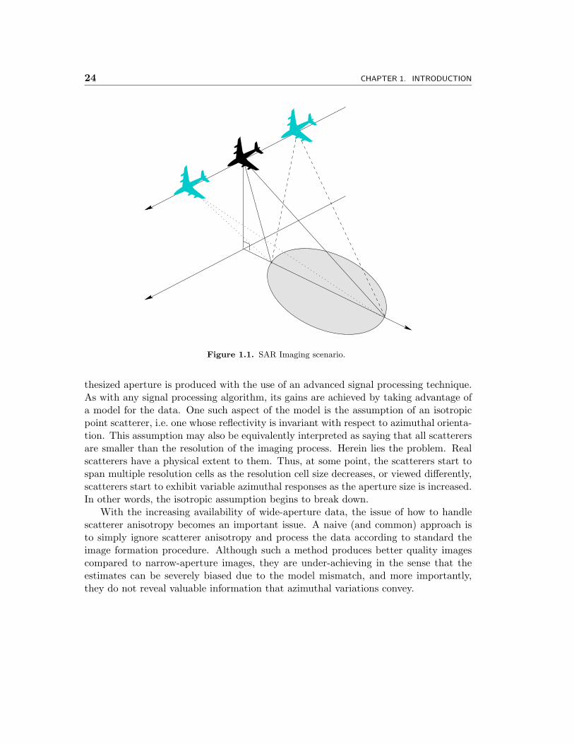
Synthetic aperture radar (SAR)[17, 42, 43, 52] is a microwave radar[58] imaging sys-tem frequently used in fields such as remote sensing, surveillance, and automatic targetrecognition (ATR). Its popularity is due in large part to its ability to attain a highimaging resolution, rapidly cover large areas of terrain, supply its own illumination, andoperate in inclement weather. The SAR imaging scenario is illustrated in Figure 1.1where a radar is mounted on an airborne or spaceborne craft and takes multiple mea-surements of a scene. In conventional radar, the cross-range resolution is the width ofthe shaded footprint illustrated. This width is proportional to the distance between theradar and the target area; and, it is inversely proportional to the size of the antenna.SAR achieves a high resolution by effectively manipulating the latter. In particular,it uses the measurements taken from the different positions along the flight path andfuses them together to synthesize an aperture the length of the integrated flight path,thus producing higher fidelity and higher resolution imagery than that of conventionalradar imaging.
The application for SAR by which this thesis is motivated is ATR[8, 9, 23]. Thisinvolves using attributes of the SAR data to classify the contents of the image scene.Any ATR algorithm can be loosely regarded as a feature extraction and comparisonprocess. The features may be as simple as the reflectivity value at each pixel, e.g. asused in simple image correlation techniques[56]. They may also be as complicated asprecise descriptions of the geometrical structure of the target[25, 34, 13] or as abstracttransformations of the data which do not have a clear physical interpretation[10]. Amotif of this thesis is the development of a feature to be used in ATR which providesboth distinguishing information for discrimination and a physically meaningful inter-pretation. The need for the former is clear in that the feature should help differentiatevarious targets of interest. The latter is useful because it allows for an intuitive un-derstanding of what information the feature represents thus guiding its use in ATRalgorithms. Furthermore, although the proposed features are designed with ATR inmind, the information they convey is useful in many other contexts due to their physi-cal interpretation.
The features with which this thesis is concerned are motivated by a shortcoming ofstandard SAR imaging. As technology progresses, the desire for higher resolution im-agery drives the development of SAR systems with larger synthetic apertures. The syn-
23
24 CHAPTER 1. INTRODUCTION
✈✈
✈
Figure 1.1. SAR Imaging scenario.
thesized aperture is produced with the use of an advanced signal processing technique.As with any signal processing algorithm, its gains are achieved by taking advantage ofa model for the data. One such aspect of the model is the assumption of an isotropicpoint scatterer, i.e. one whose reflectivity is invariant with respect to azimuthal orienta-tion. This assumption may also be equivalently interpreted as saying that all scatterersare smaller than the resolution of the imaging process. Herein lies the problem. Realscatterers have a physical extent to them. Thus, at some point, the scatterers start tospan multiple resolution cells as the resolution cell size decreases, or viewed differently,scatterers start to exhibit variable azimuthal responses as the aperture size is increased.In other words, the isotropic assumption begins to break down.
With the increasing availability of wide-aperture data, the issue of how to handlescatterer anisotropy becomes an important issue. A naive (and common) approach isto simply ignore scatterer anisotropy and process the data according to standard theimage formation procedure. Although such a method produces better quality imagescompared to narrow-aperture images, they are under-achieving in the sense that theestimates can be severely biased due to the model mismatch, and more importantly,they do not reveal valuable information that azimuthal variations convey.
Sec. 1.1. Premise 25
� 1.1 Premise
This thesis is based on the premise that scatterer anisotropy is present and exploitablein SAR. Not only is scatterer anisotropy predicted by scattering physics[48, 61], but ithas also been observed in real data[2, 12, 51]. Neglecting anisotropy naturally leads tosuboptimal use of the SAR data due to the model mismatch as demonstrated by Yeanget. al.[61].
Scatterer anisotropy need not degrade SAR quality. In fact, it can offer significantimprovements to SAR imaging and ATR. From an imaging standpoint, a better scat-tering model allows for more accurate reflectivity estimates since the weighting in theimage formation process can be adjusted according to the azimuthal scattering pat-tern (e.g. with a matched filter). Knowledge of anisotropy may also be used to bettersuppress interfering scatterers in super-resolution image formation algorithms. In ad-dition to improving reflectivity estimation, knowledge of the anisotropy of a scattereris useful as a feature in and of itself. For a canonical scatterer, one can infer propertiesabout its geometric shape and size from its anisotropy. Knowledge of the geometry ofthe individual scatterers on an object may then be considered in tandem to aid theclassification of the target under investigation. Anisotropy information may also beuseful to characterize the stability of a scatterer. In particular, the specular responsefrom an anisotropic canonical scatterer appears over a smaller range in azimuth leadingto an observability that is more sensitive to azimuthal orientation. Knowledge of thisanisotropy however allows such sensitivity to be incorporated into algorithms such aspeak matching which should improve ATR performance.
� 1.2 Previous Efforts
Previous efforts to deal with scatterer anisotropy in SAR can loosely be divided intotwo categories: those which are based on precise canonical scattering models and thosebased on the more general sub-aperture scattering models. Physical optics (PO)[48]and the geometric theory of diffraction (GTD)[33] give accurate predictions of the scat-terer response for what are called canonical or atomic scatterers. These are scatteringprimitives which have very simple geometries and include as examples the flat plate,cylinder, sphere, top-hat, dihedral, and trihedral.
Canonical scattering models are a natural tool for exploiting scatterer anisotropydue to their precise modeling. Their application in SAR has generally fallen into oneof two classes. The first is their use to estimate the canonical type and the associ-ated parameters of scatterers in SAR data. Moses, Potter, and Chiang take such anapproach where they use GTD models. Potter and Moses[45], use a maximum likeli-hood framework to estimate the scatterer type and associated parameters from imagedata. This work is extended by Chiang[13] to evaluate the improvement in SAR ATRperformance that such estimates could provide. McClure and Carin[40] have also usedcanonical models to estimate the scatterer type and associated parameters. In theirapproach, they populate a “dictionary” of basis functions with the GTD responses for
26 CHAPTER 1. INTRODUCTION
various scatterers of interest in addition to other families of models1. They use thisdictionary of basis functions in a matching-pursuit framework to decompose SAR datainto constituent scatterers. In the mentioned approaches, very high fidelity data isnecessary for accurate estimation. This is required because over a single image, it isoften difficult to differentiate responses from different geometrical configurations. Per-formance degrades even more so in the presence of interfering scatterers. Richards[46]addresses this problem in a context in which many images from various orientationsare available such as in an automated target model generation framework. He usesthe iterative expectation-maximization algorithm to perform scatterer correspondenceamong the various images and to estimate the parameters of each of the scatterers.The use of a large amount of observation data in this approach successfully allows foraccurate estimation of the scatterers.
The success of the approaches mentioned in the previous paragraph depends heavilyon the availability of large amounts of data or high fidelity data with little interferenceamong scatterers. However, it is often the task in ATR to classify an object using onlyone or a few images which contain many scatterers. This motivates the other, less ambi-tious, use of canonical models which is to use them to improve the images of reflectivityestimates. Benitz[4, 7, 5] takes this approach by employing canonical scatterer modelsin super-resolution methods. In particular, he uses a canonical scatterer response asthe model in a variant on Capon’s method and in the MUSIC algorithm. The result isan image of reflectivities specifically tuned for the model scatterer. Because the imageis tuned for a particular scatterer, this imaging process is performed for a series ofpre-specified scatterer geometries thus giving rise to a vector of images or what Benitzcalls high definition vector imaging (HDVI).
Chaney et. al.[12] and Allen et. al.[2] follow approaches similar in spirit to Benitz’smethods but with some significant differences. Allen and Chaney are both concernedwith low-frequency SAR which has a lower resolution where only large scatterers, mea-suring on the order of a meter or more, are apparent in the imagery. For a vehicle,these scatterers are typically the broadside response associated with the front, back, orside of the target. However, tree trunks also produce strong responses. Allen uses thedifferences in azimuthal dependencies between the flat plate and the cylindrical treetrunk to differentiate the two. He does so using a bank of approximate matched filtersto generate reflectivity estimates. The matched filters are approximate in the sensethat they are based on sub-aperture scattering models, i.e. models which assume theazimuthal response is uniform over a section of the aperture and zero elsewhere. Inparticular, he uses a sequence of overlapping sub-apertures each of which has the samelength. Allen uses the resulting sub-aperture reflectivity estimates in two ways. First, todistinguish a vehicle’s broadside response from a tree trunk’s isotropic response, Allenuses the maximum sub-aperture reflectivity to characterize the scatterer. Although theflat plate and tree trunk produce similar reflectivities when the entire aperture is used,
1Besides the canonical scatterer models, McClure and Carin use resonance models to account forcavities and chirp models to account for dispersive structures.
Sec. 1.2. Previous Efforts 27
the flat plate produces a very directive response resulting in a very strong response con-centrated in a few of the sub-apertures, whereas the tree trunk produces an isotropicresponse resulting in a constant but smaller reflectivity among all the sub-apertures.Thus, the vehicle appears significantly brighter than trees in Allen’s image of maximumsub-aperture reflectivities. Allen also uses the sub-aperture reflectivities to estimatethe azimuthal location and width of the directive flat plate response. He does so byplotting the sub-aperture reflectivities as the sub-apertures transition from one end ofthe aperture to the other thus displaying how the response varies in azimuth. Thecharacteristics of the directive response are then measured from this plot.
Chaney independently takes an approach similar to Allen’s. In particular, Chaneyforms a series of sub-aperture reflectivity estimates and chooses the sub-aperture pro-ducing the maximum estimate. Doing this for every pixel, Chaney obtains an imageof matched reflectivity estimates. The most significant difference between Allen’s andChaney’s approaches is that Chaney varies the size the sub-aperture to adapt to theazimuthal width of the response, whereas Allen uses a fixed pre-specified azimuthalwidth. Varying the size of the sub-aperture, however, also produces reflectivity esti-mates with different spatial resolutions. Thus, to limit the artifacts that such changesmay produce in the image, Chaney also regularizes the sub-aperture selection to limitthe fluctuations as one moves throughout the image.
There are two primary differences between the approach taken by Benitz and thosetaken by Allen and Chaney. The first is that Allen and Chaney use the simpler sub-aperture scattering model and are thus not overwhelmed by the myriad images theyneed to generate. They are only concerned with the gross-level scatterer anisotropywhich one can observe. The second difference is that Benitz provides a vector of images(one image of estimates under each scatterer model), whereas Allen and Chaney providea single image (choosing a single estimate from among all the models). The latter ismore amenable to direct inclusion into existing image based ATR algorithms, but thefashion in which the estimate is chosen leads to sub-optimal resolution. In particular,Allen uses sub-apertures of a pre-specified length, thus imposing a fixed resolutionwhich is not adapted to individual scatterers. Chaney, in contrast, uses sub-aperturesof varying lengths, and, for each pixel, selects the sub-aperture which produces themaximum reflectivity estimate. This approach, however, leads to an excessively coarseresolution because the method neglects the higher noise variance in smaller sub-apertureestimates. In particular because the sub-aperture reflectivity estimate from too smallan aperture has an unbiased error, the higher noise variance increases the probabilitythat the maximum reflectivity is produced in one of the smaller sub-apertures.
Smith[51] takes an approach similar to Allen’s by dividing the full-aperture intooverlapping sub-apertures of constant length. However, instead of looking to detectand measure anisotropy from canonical scatterers, Smith’s goal is to characterize thestability of the scatterer. In particular, for each peak location determined through aseparate peak extraction step, a number is assigned to the scatterer characterizing thefluctuations of the sub-aperture reflectivities. This peak stability is then used as a
28 CHAPTER 1. INTRODUCTION
confidence measure for that scatterer in a peak matching classification algorithm. Thisstability weighting is motivated by the idea that more stable peaks (i.e. those whichexhibit less azimuthal variation) should be weighted more heavily since they are morelikely to be matched in another image of the target. Although this thesis argues thatanisotropy is useful and should not be discarded, Smith’s approach is reasonable in itscontext of application to existing ATR peak matching algorithms which use standardSAR image formation based on the isotropic scattering assumption.
Subotic et. al.[53] have also worked with sub-aperture models, but not in the contextof anisotropy. In his work, he examines the reflectivities produced by a nested sequenceof sub-apertures. Treating the sequence as a multi-scale process, he then examinesseveral statistical tests for the detection of isotropic scatterers. Subotic’s contributionis significant because of its specific focus on how the varying size of the resolution cellimpacts the statistical behavior of the reflectivity estimates. All of the other methodsmentioned in this section do not address this issue with the exception of Chaney whoaddresses it indirectly by regularizing the sub-aperture selection process.
Irving et. al.[31] has also proposed modeling SAR data as a multi-scale stochasticprocess. Instead of varying the size of the sub-aperture to change the resolution, Irvingcoherently averages 2 × 2 pixel blocks in a recursive fashion to generate a quad-treerepresentation of the SAR data. He then uses an auto-regressive model in scale todescribe the behavior of the log-magnitude of the reflectivities on the quad-tree. Thisis motivated by the idea that clutter is composed of many small independent scatter-ers and thus should have little scale-to-scale dependence because the random phaseson each of the scatterers cause them to interfere with each other in a chaotic fashionas resolution is varied. In contrast, larger scattering objects, such as trees or targets,should demonstrate strong scale-to-scale dependence as they share a common phase overthe scatterer and thus constructively interfere to produce a stronger response as scaleis coarsened. Multi-scale modeling is thus used by Irving to differentiate anomalousman-made targets from natural clutter according to their scale auto-regressive behav-ior. This idea is also used for terrain segmentation by Fosgate et. al.[24] where grassand forest terrain are differentiated based on their respective multi-scale dependencies.Fosgate also proposes a multi-scale anomaly detector to detect the extremely high scale-to-scale correlation that is characteristic of man-made targets. Kim et. al.[36] enhancesthe segmentation algorithm of Fosgate by incorporating model deviations and subse-quently develops a segmentation-based compression algorithm exploiting the revealeddependencies for each terrain class.
� 1.3 Thesis Objective
The results of both Allen and Chaney demonstrate that anisotropy can be used toimprove ATR performance on acquired SAR data. This thesis builds upon their sub-aperture analysis to develop robust methods to exploit scatterer anisotropy in ATR.In particular, we present a more robust representation of the data and a statistical
Sec. 1.3. Thesis Objective 29
framework which improves upon that of Allen and Chaney by providing more accurateanisotropy characterizations and higher resolution imagery.
The first main issue to be addressed in this thesis is that of data representation.While it is theoretically true that any invertible transformation of the data is equallysuitable for subsequent estimation, the packaging of the data significantly impacts theclarity and practical implementation of the estimation. For the case of SAR, thereis a fundamental trade-off in being able to obtain measurements with high azimuthalresolution (i.e. the ability to observe azimuthal variations) and high imaging resolution.The methods mentioned in the previous section do not directly address this issue andthus suffer from this trade-off as they must exchange one form of resolution for theother. However, this thesis proposes a multi-resolution pyramid representation of theSAR data at a variety of resolution trade-offs that permits a decision-directed approachwhich produces estimates with both high imaging and azimuthal resolution.
Having addressed the first issue of data representation, this thesis proceeds to itsprimary goal of exploiting anisotropy for ATR. Even with the sub-aperture representa-tion in place, there are still issues which require consideration. First, there is the issueof how anisotropy is to be exploited to aid ATR. Two approaches are taken towardsthis end. One is to apply machine learning to solve the classification problem. In thisapproach, the anisotropy dependencies conditioned on a particular target classes arelearned via a nonparametric estimator. The learned densities are then directly usedto implement a classifier. The drawback to this approach is that it limits the degreeto which physical modeling and intuition can be leveraged to analyze and improve theclassifier. In particular, the learned densities are driven by the data and do not conveyobvious physical information about the target. Thus, the role which an ATR analyst canplay is limited. This motivates the second approach to improving ATR which extendsthe efforts of Allen and Chaney. In particular, the sub-aperture scattering model isused to describe the concentration of scattering in azimuth. An optimal sub-aperture ischosen and subsequently used to provide an enhanced reflectivity estimate. In additionto the sub-aperture reflectivity estimates, the specifics about the chosen sub-apertureare also provided to convey information about the geometry of the scatterer. The ef-forts of Allen and Chaney are extended in three significant ways. The first is that theirmodel for the sub-aperture measurements is improved upon thereby producing a moreaccurate test. The second improvement is that the structure of the sub-aperture pyra-mid is leveraged to obtain both high imaging and high azimuthal resolution throughthe use of a decision-directed procedure exploiting the presence of multiple resolutions.The third extension is that the effects of neighboring scatterers are included in ouranalysis. Addressing the issue of interfering scatterers is essential as they corrupt theobserved azimuthal response resulting in anisotropy misclassifications and, in effect,reduced spatial resolution when ignored.
30 CHAPTER 1. INTRODUCTION
� 1.4 Thesis Organization
The remainder of this thesis addresses these issues and is organized as follows.
� 1.4.1 Background
Chapter 2 provides the necessary background in SAR and machine learning needed toaddress the issues of concern in this thesis. The chapter begins by discussing the fun-damentals of SAR. Such details are important in that the processing used to achieveSAR’s high resolution are strongly based on the ideal point-scattering model which ig-nores scatterer anisotropy. SAR image formation is also presented from a beamformingperspective which allows the inclusion of models other than the ideal point scatterermodel. The chapter concludes with a description of nonparametric density estimationand how it can be used for classification.
� 1.4.2 Sub-aperture Analysis
Chapter 3 introduces the sub-aperture pyramid which serves as the fundamental struc-ture for all of the analysis in this thesis. In this structure, the sub-apertures are arrangedin a pyramidal fashion according to their size and azimuthal location. The sub-aperturepyramid is used both to estimate reflectivity and define the models for anisotropy. Theframework can be interpreted in a multi-scale setting, where each scale provides a dif-ferent azimuthal versus spatial resolution trade-off. This structure is also viewed in thecontext of other works. In particular, it can be seen as
• a multiple-basis representation offering different tilings of the azimuthal-imageplane2 a la wavelet packet dictionaries[59].
• an extension of the sub-aperture work by Allen and Chaney,
• an instance of the vector imaging work by Benitz,
� 1.4.3 Nonparametric Estimation of Anisotropy
Chapter 4 presents an extension of the nonparametric approach of DeBonet et. al.[20].The fundamental change is the use of the sub-aperture pyramid motivated by scatteringphysics in contrast to steerable wavelets motivated by visual attributes. Because thesub-aperture scattering model approximates the aspect dependent scattering producedby canonical scatterers, the sub-aperture pyramid captures such responses in a clearmanner. The advantage of this machine learning approach is that data dependencies areautomatically learned with a nonparametric estimator. However, there are several issuesconcerning the implementation of this nonparametric approach which are addressed inthis chapter. Classification performance is measured and analyzed with the MSTAR[1]data set.
2This is traditionally called the time-frequency plane in signal processing, but is not done so here toprevent confusion with SAR terminology.
Sec. 1.4. Thesis Organization 31
� 1.4.4 Sub-aperture Anisotropy Attribution
Chapter 5 deals with the topic of attributing a given spatial pixel with an anisotropy la-bel and associated reflectivity estimate. Allen and Chaney choose the sub-aperture withmaximum reflectivity because of its matched-filter interpretation. However, Allen im-poses a pre-specified sub-aperture size and thus cannot adapt the sub-aperture to matchthe width of the azimuthal response. Chaney, in contrast, varies the sub-aperture size,but he does not account for the resulting change in the sub-aperture noise variance.Based on the sub-aperture pyramid, a consistent statistical model and test for sub-aperture anisotropy are presented. The result is an intuitively simple test providingbetter imaging resolution and more accurate anisotropy labels than Allen and Chaney.The anisotropy characterization also reveals why the sub-aperture selection used byAllen and Chaney leads to an excessively coarse imaging resolution. Several modifi-cations on the proposed anisotropy test are discussed. The first modification changesthe estimation of an auxiliary parameter to address the lack of an explicit model forinterfering scatterers which distort the azimuthal response and hence the classification.The second modification also addresses the issue of interfering scatterers but does sothrough a telescopic decision-directed testing procedure on the sub-aperture pyramidwhich also reduces computational complexity. The third modification addresses devi-ations from the sub-aperture scattering models through a model perturbation term.Results demonstrating the utility provided by the anisotropy attribution are providedon the MSTAR data set.
� 1.4.5 Anisotropy Phenomenology
The results on MSTAR data at the end of Chapter 5 strongly argue for two differentsources of anisotropy. The study of these two modes is the topic of Chapter 6. Thesetwo classes are called geometric and volumetric scatterers. Geometric scatterers arelarge structured scatterers such as canonical scatterers and scatterers with slight devia-tions from canonicity. Volumetric scatterers on the other hand are actually a collectionof many unresolvable scatterers which happen to coherently combine to produce ananisotropic response over the observed azimuth. Not surprisingly, anisotropy from vol-umetric scatterers is not stable due to the chaotic nature of its azimuthal response, andthus it provides no utility to ATR. Anisotropy from geometric scatterers is however verystable and provides significant information about the underlying scatterer, and thus itprovides significant utility for ATR. Unfortunately, it is difficult, if not impossible, todetermine the source of anisotropy based on a single observation from moderate reso-lution (i.e. moderate aperture) SAR. However, the use of wide-aperture SAR decreasesthe incidence of anisotropy from volumetric scatterers by utilizing the increased rangeof azimuthal data to assess the stability3 of the azimuthal response.
3This notion of azimuthal stability is more general than that of Smith’s[51] who considers devia-tions from the point scattering model as compared to deviations from canonical anisotropic responsesconsidered in this thesis.
32 CHAPTER 1. INTRODUCTION
� 1.4.6 Iterative Anisotropy Attribution
Chapter 7 returns to the topic of anisotropy attribution by improving the modeling andestimation proposed in Chapter 5. In particular, this chapter extends the modeling ofneighboring scatterers by allowing the consideration of anisotropic neighbors. Ratherthan attempting the monumental task of simultaneously estimating the anisotropy ofall the pixels, an iterative approach is taken in which the azimuthal contributions fromneighboring scatterers is modeled using the anisotropy classification from the previousiteration. Special care must be taken in using the information from the previous iter-ation so as to appropriately account for the contributions from neighboring scatterers.In particular, a distinction must be made between pixels and scatterers. Consider forexample, removing the azimuthal distortion produced by a physically large interfer-ing scatterer that spans several, say N , pixels. If one were to simply subtract off itseffect for every pixel, then that would be equivalent to saying that there are N scat-terers exhibiting this response (one for each of the pixel locations) instead of the oneunderlying scatterer. Thus, the modeling of neighboring scatterers must be carefullytaken into account in order to prevent over-compensating for their azimuthal distor-tion. While it is necessary to remove the interference from neighboring scatterers, theeffects from on-scatterer pixels should be preserved. On-scatterer pixels are pixels cor-responding to the same scatterer as the pixel being examined. If their contribution isremoved, then another form of distortion is introduced which cancels part of the re-sponse from the scatterer in question thus corrupting the anisotropy classification. Inorder to address these issues, an additional processing step is used which aggregatespixels into their underlying scatterers. The segmentation algorithm used is based ona greedy maximum-likelihood algorithm. The segmentation is then used to distinguishoff-scatterer pixels from on-scatterer pixels so that only the contribution from interfer-ing scatterers are removed. The chapter concludes with a presentation of experimentalresults demonstrating the performance of both the anisotropy attribution and scatterersegmentation.
� 1.4.7 Conclusions
The thesis concludes with Chapter 8. A summary of the contributions in this thesisis first provided. This is followed by a discussion of opportunities for future researchutilizing or extending the anisotropy analysis we have developed.
Chapter 2
Background
The work in this thesis focuses on the development of techniques that exploit non-ideal scattering in synthetic aperture radar (SAR) imagery for the purpose of targetrecognition. In this background chapter, the fundamentals describing relevant areas ofSAR and machine learning are presented. These are broad topics incapable of beingsummarized in a single chapter. Focus is thus restricted to those aspects which aremost pertinent to the work in this thesis. Section 2.1 presents the fundamentals of con-ventional SAR image formation. Section 2.2 describes SAR from a spectral estimationperspective motivated by array processing which helps provide intuition about SAR.Section 2.3 discusses the issue of nonideal scattering along with some current efforts toaddress it. Section 2.4 concludes the chapter with a discussion of nonparametric den-sity estimation and how it can be used for the problem of classification. A footnote foreach sub-section heading indicates the bibliographical sources from which the materialis obtained and where more details may be found.
� 2.1 Conventional SAR
Active radar imaging systems are frequently used in remote sensing and surveillanceapplications. SAR is a special case of microwave radar imaging that uses sophisti-cated signal processing to achieve a high imaging resolution. In the SAR scenario, aradar is mounted on an airborne or spaceborne craft where it illuminates the regionof interest and measures the corresponding reflectivity. Using a microwave band radarsystem has several advantages. Since it is an active imaging system, it provides itsown illumination in the form of microwave radiation, thus allowing it to be used forboth day and night operation. Furthermore, because microwave radiation is not sig-nificantly attenuated by atmospheric components such as common gases, dense fog, orcloud cover, microwave-frequency radar systems produce images that are unimpairedby such natural phenomena.
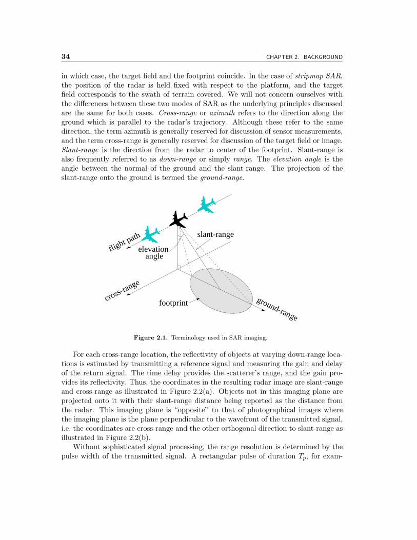
The radar imaging scenario is illustrated in Figure 2.1 along with some commonlyused terms. The footprint refers to the ground area illuminated by the radar andrepresents the region for which the reflectivity is being measured. The target field is thecumulative area covered by the footprint as the radar is moved. In the case of spotlightSAR, the radar is continuously steered such that the area of illumination is constant,
33
34 CHAPTER 2. BACKGROUND
in which case, the target field and the footprint coincide. In the case of stripmap SAR,the position of the radar is held fixed with respect to the platform, and the targetfield corresponds to the swath of terrain covered. We will not concern ourselves withthe differences between these two modes of SAR as the underlying principles discussedare the same for both cases. Cross-range or azimuth refers to the direction along theground which is parallel to the radar’s trajectory. Although these refer to the samedirection, the term azimuth is generally reserved for discussion of sensor measurements,and the term cross-range is generally reserved for discussion of the target field or image.Slant-range is the direction from the radar to center of the footprint. Slant-range isalso frequently referred to as down-range or simply range. The elevation angle is theangle between the normal of the ground and the slant-range. The projection of theslant-range onto the ground is termed the ground-range.
✈footprint
flight path
✈✈
ground-range
cross-range
slant-range
angleelevation
Figure 2.1. Terminology used in SAR imaging.
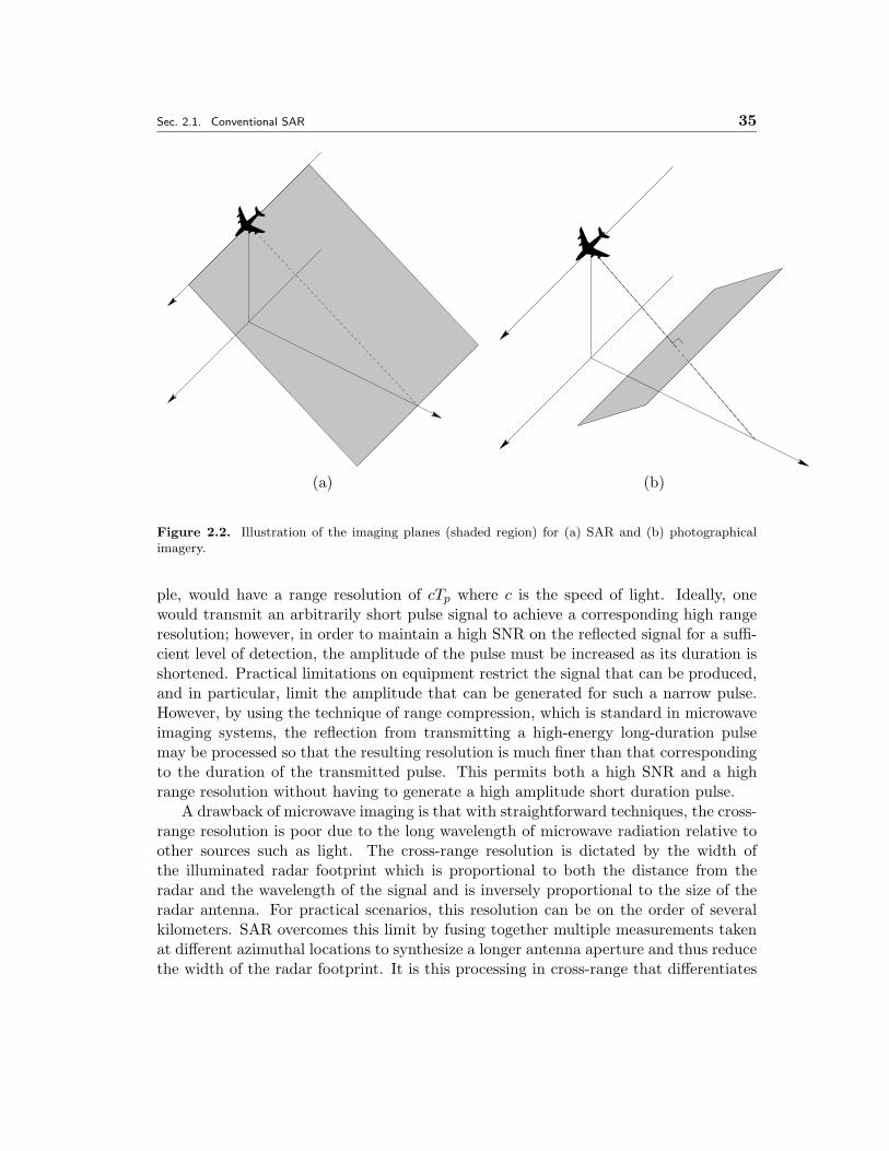
For each cross-range location, the reflectivity of objects at varying down-range loca-tions is estimated by transmitting a reference signal and measuring the gain and delayof the return signal. The time delay provides the scatterer’s range, and the gain pro-vides its reflectivity. Thus, the coordinates in the resulting radar image are slant-rangeand cross-range as illustrated in Figure 2.2(a). Objects not in this imaging plane areprojected onto it with their slant-range distance being reported as the distance fromthe radar. This imaging plane is “opposite” to that of photographical images wherethe imaging plane is the plane perpendicular to the wavefront of the transmitted signal,i.e. the coordinates are cross-range and the other orthogonal direction to slant-range asillustrated in Figure 2.2(b).
Without sophisticated signal processing, the range resolution is determined by thepulse width of the transmitted signal. A rectangular pulse of duration Tp, for exam-
Sec. 2.1. Conventional SAR 35
✈ ✈
(a) (b)
Figure 2.2. Illustration of the imaging planes (shaded region) for (a) SAR and (b) photographicalimagery.
ple, would have a range resolution of cTp where c is the speed of light. Ideally, onewould transmit an arbitrarily short pulse signal to achieve a corresponding high rangeresolution; however, in order to maintain a high SNR on the reflected signal for a suffi-cient level of detection, the amplitude of the pulse must be increased as its duration isshortened. Practical limitations on equipment restrict the signal that can be produced,and in particular, limit the amplitude that can be generated for such a narrow pulse.However, by using the technique of range compression, which is standard in microwaveimaging systems, the reflection from transmitting a high-energy long-duration pulsemay be processed so that the resulting resolution is much finer than that correspondingto the duration of the transmitted pulse. This permits both a high SNR and a highrange resolution without having to generate a high amplitude short duration pulse.
A drawback of microwave imaging is that with straightforward techniques, the cross-range resolution is poor due to the long wavelength of microwave radiation relative toother sources such as light. The cross-range resolution is dictated by the width ofthe illuminated radar footprint which is proportional to both the distance from theradar and the wavelength of the signal and is inversely proportional to the size of theradar antenna. For practical scenarios, this resolution can be on the order of severalkilometers. SAR overcomes this limit by fusing together multiple measurements takenat different azimuthal locations to synthesize a longer antenna aperture and thus reducethe width of the radar footprint. It is this processing in cross-range that differentiates
36 CHAPTER 2. BACKGROUND
SAR from other microwave imaging systems. In the remainder of this section, thetechniques used to achieve high range and cross-range resolution are described.
� 2.1.1 Matched Filter Range Compression 1
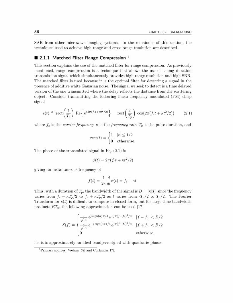
This section explains the use of the matched filter for range compression. As previouslymentioned, range compression is a technique that allows the use of a long durationtransmission signal which simultaneously provides high range resolution and high SNR.The matched filter is used because it is the optimal filter for detecting a signal in thepresence of additive white Gaussian noise. The signal we seek to detect is a time delayedversion of the one transmitted where the delay reflects the distance from the scatteringobject. Consider transmitting the following linear frequency modulated (FM) chirpsignal
s(t) � rect(
t
Tp
)Re{ej2π(fct+κt2/2)
}= rect
(t
Tp
)cos
(2π(fct+ κt2/2)
)(2.1)
where fc is the carrier frequency, κ is the frequency rate, Tp is the pulse duration, and
rect(t) =
{1 |t| ≤ 1/20 otherwise.
The phase of the transmitted signal in Eq. (2.1) is
φ(t) = 2π(fct+ κt2/2)
giving an instantaneous frequency of
f(t) =12π
d
dtφ(t) = fc + κt.
Thus, with a duration of Tp, the bandwidth of the signal is B = |κ|Tp since the frequencyvaries from fc − κTp/2 to fc + κTp/2 as t varies from -Tp/2 to Tp/2. The FourierTransform for s(t) is difficult to compute in closed form, but for large time-bandwidthproducts BTp, the following approximation can be used [17]
S(f) =
1√|κ| e
j sign(κ)π/4 e−jπ(f−fc)2/κ |f − fc| < B/21√|κ| e
−j sign(κ)π/4 ejπ(f−fc)2/κ |f + fc| < B/2
0 otherwise,
i.e. it is approximately an ideal bandpass signal with quadratic phase.1Primary sources: Wehner[58] and Curlander[17].
Sec. 2.1. Conventional SAR 37
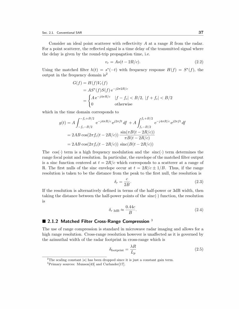
Consider an ideal point scatterer with reflectivity A at a range R from the radar.For a point scatterer, the reflected signal is a time delay of the transmitted signal wherethe delay is given by the round-trip propagation time, i.e.
vr = As(t− 2R/c). (2.2)
Using the matched filter h(t) = s∗(−t) with frequency response H(f) = S∗(f), theoutput in the frequency domain is2
G(f) = H(f)Vr(f)
= AS∗(f)S(f) e−j2π2R/c
=
{A e−j4πR/c |f − fc| < B/2, |f + fc| < B/20 otherwise
which in the time domain corresponds to
g(t) = A
∫ −fc+B/2
−fc−B/2e−j4πR/c ej2πft df +A
∫ fc+B/2
fc−B/2e−j4πR/c ej2πft df
= 2AB cos(2πfc(t− 2R/c))sin(πB(t− 2R/c))πB(t− 2R/c)
= 2AB cos(2πfc(t− 2R/c)) sinc(B(t− 2R/c))
The cos(·) term is a high frequency modulation and the sinc(·) term determines therange focal point and resolution. In particular, the envelope of the matched filter outputis a sinc function centered at t = 2R/c which corresponds to a scatterer at a range ofR. The first nulls of the sinc envelope occur at t = 2R/c ± 1/B. Thus, if the rangeresolution is taken to be the distance from the peak to the first null, the resolution is
δr =c
2B. (2.3)
If the resolution is alternatively defined in terms of the half-power or 3dB width, thentaking the distance between the half-power points of the sinc(·) function, the resolutionis
δr 3dB ≈ 0.44cB
. (2.4)
� 2.1.2 Matched Filter Cross-Range Compression 3
The use of range compression is standard in microwave radar imaging and allows for ahigh range resolution. Cross-range resolution however is unaffected as it is governed bythe azimuthal width of the radar footprint in cross-range which is
δfootprint =λR
Lp(2.5)
2The scaling constant |κ| has been dropped since it is just a constant gain term.3Primary sources: Munson[43] and Curlander[17].
38 CHAPTER 2. BACKGROUND
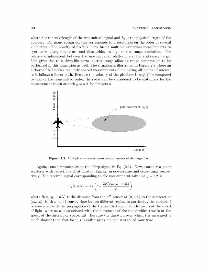
where λ is the wavelength of the transmitted signal and Lp is the physical length of theaperture. For many scenarios, this corresponds to a resolution on the order of severalkilometers. The novelty of SAR is in its fusing multiple azimuthal measurements tosynthesize a larger aperture and thus achieve a higher cross-range resolution. Therelative displacement between the moving radar platform and the stationary targetfield gives rise to a chirp-like term in cross-range allowing range compression to beperformed in this dimension as well. The situation is illustrated in Figure 2.3 where anairborne SAR makes regularly spaced measurements illuminating all points of interestas it follows a linear path. Because the velocity of the platform is negligible comparedto that of the transmitted pulse, the radar can be considered to be stationary for themeasurement taken at each y = n∆ for integers n.
0 0(x ,y )
∆
✈
Range (x)
Cro
ss R
ange
(y)
✴
point scatterer at
Figure 2.3. Multiple cross-range sensor measurements of the target field.
Again, consider transmitting the chirp signal in Eq. (2.1). Now, consider a pointscatterer with reflectivity A at location (x0, y0) in down-range and cross-range respec-tively. The received signal corresponding to the measurement taken at y = n∆ is
vr(t, n∆) = As
(t− 2R(x0, y0 − n∆)
c
)where R(x0, y0 − n∆) is the distance from the nth sensor at (0, n∆) to the scatterer at(x0, y0). Both n and t convey time but on different scales. In particular, the variable tis associated with the propagation of the transmitted signal which travels at the speedof light, whereas n is associated with the movement of the radar which travels at thespeed of the aircraft or spacecraft. Because the duration over which t is measured ismuch shorter than that for n, t is called fast time and n is called slow time.
Sec. 2.1. Conventional SAR 39
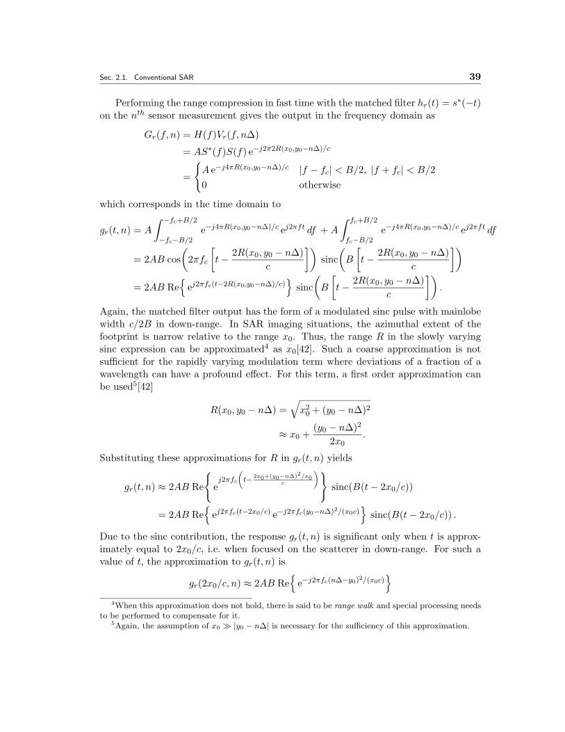
Performing the range compression in fast time with the matched filter hr(t) = s∗(−t)on the nth sensor measurement gives the output in the frequency domain as
Gr(f, n) = H(f)Vr(f, n∆)
= AS∗(f)S(f) e−j2π2R(x0,y0−n∆)/c
=
{A e−j4πR(x0,y0−n∆)/c |f − fc| < B/2, |f + fc| < B/20 otherwise
which corresponds in the time domain to
gr(t, n) = A
∫ −fc+B/2
−fc−B/2e−j4πR(x0,y0−n∆)/c ej2πft df +A
∫ fc+B/2
fc−B/2e−j4πR(x0,y0−n∆)/c ej2πft df
= 2AB cos(2πfc
[t− 2R(x0, y0 − n∆)
c
])sinc
(B
[t− 2R(x0, y0 − n∆)
c
])= 2AB Re
{ej2πfc(t−2R(x0,y0−n∆)/c)
}sinc
(B
[t− 2R(x0, y0 − n∆)
c
]).
Again, the matched filter output has the form of a modulated sinc pulse with mainlobewidth c/2B in down-range. In SAR imaging situations, the azimuthal extent of thefootprint is narrow relative to the range x0. Thus, the range R in the slowly varyingsinc expression can be approximated4 as x0[42]. Such a coarse approximation is notsufficient for the rapidly varying modulation term where deviations of a fraction of awavelength can have a profound effect. For this term, a first order approximation canbe used5[42]
R(x0, y0 − n∆) =√
x20 + (y0 − n∆)2
≈ x0 +(y0 − n∆)2
2x0.
Substituting these approximations for R in gr(t, n) yields
gr(t, n) ≈ 2AB Re
{ej2πfc
(t− 2x0+(y0−n∆)2/x0
c
)}sinc(B(t− 2x0/c))
= 2AB Re{ej2πfc(t−2x0/c) e−j2πfc(y0−n∆)2/(x0c)
}sinc(B(t− 2x0/c)) .
Due to the sinc contribution, the response gr(t, n) is significant only when t is approx-imately equal to 2x0/c, i.e. when focused on the scatterer in down-range. For such avalue of t, the approximation to gr(t, n) is
gr(2x0/c, n) ≈ 2AB Re{e−j2πfc(n∆−y0)2/(x0c)
}4When this approximation does not hold, there is said to be range walk and special processing needs
to be performed to compensate for it.5Again, the assumption of x0 � |y0 − n∆| is necessary for the sufficiency of this approximation.
40 CHAPTER 2. BACKGROUND
which is similar in form to a delayed version of the transmitted chirp in Eq. (2.1) withthe time variable denoted as n∆, a carrier frequency of 0, and a frequency rate of−2fc/(x0c). A rect(·) function is absent from the above equation for gr(2x0/c, n), soinstead of processing it with a matched filter (spanning all n), it is cross correlated witha windowed version of the chirp signal. This filter is
ha(n;x0) = Re{ej2πfcn2/(x0c)
}rect(n∆/La)
where La is the length of the synthetic aperture and implicitly determines the numberof cross-range measurements used since they are assumed to be uniformly spaced. Notethat the filter is parameterized with the range location, in addition to slow-time, becausethe frequency rate of the chirp in the filter varies with range to correctly focus inazimuth. Because multiple measurements are used, the effective aperture length La ismuch larger than the physical aperture, and thus the name synthetic aperture radar.
By, approximating the cross correlation of gr(2x0/c, n) with ha(n;x0) as the au-tocorrelation of ha(n;x0) and subsequently following similar steps as for the rangecompression, the time domain output becomes
gr,a(2x0/c, n) =4ABLafc
x0csinc
(2Lafcx0c
(n∆− y0)).
As for the matched filtering in range compression, when the cross-range resolution istaken as the distance between the peak of the sinc and the nearest null, this gives anazimuthal resolution of
δa =cx0
2fcLa=
λcx02La
. (2.6)
Alternatively, using the half-power bandwidth as the resolution,
δa 3dB ≈ 0.44cx0fcLa
=0.44λcx0
La. (2.7)
The expression for resolution in Eq. (2.6) is quite similar to that for conventional radarin Eq. (2.5), but note that Eq. (2.6) uses the synthesized aperture length La, which iscontrolled as a parameter, whereas Eq. (2.5) uses the physical aperture length Lp whichis limited by physical constraints.
� 2.1.3 Deramp Pulse Compression 6
This section presents a slightly different algorithm called the deramp-FFT method toapproximate the matched filter image formation for SAR data. The purpose of itsinclusion here is not because of its popularity, but more importantly, because it helpsprovide a bridge to connect SAR to ideas in spectral estimation for far field arrayprocessing. This association is further described in Section 2.2.
6Primary sources: Curlander[17] and Munson[43].
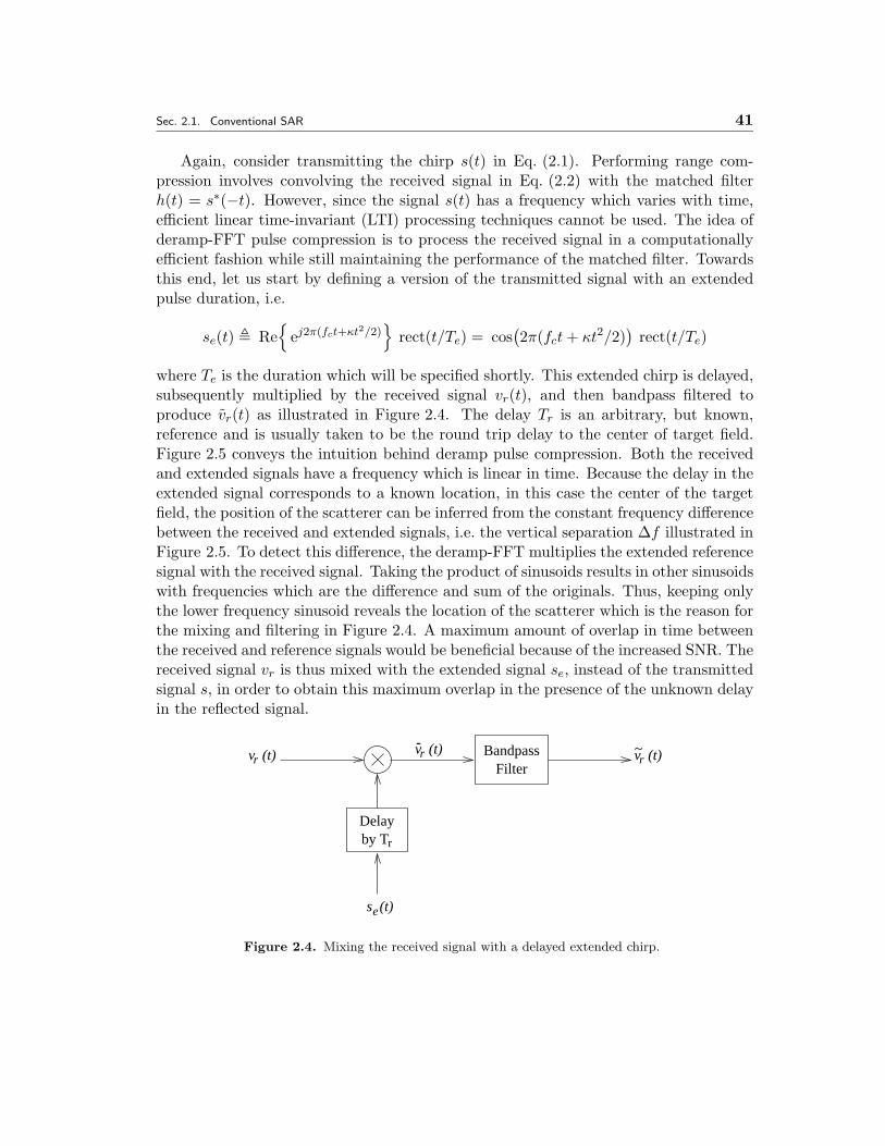
Sec. 2.1. Conventional SAR 41
Again, consider transmitting the chirp s(t) in Eq. (2.1). Performing range com-pression involves convolving the received signal in Eq. (2.2) with the matched filterh(t) = s∗(−t). However, since the signal s(t) has a frequency which varies with time,efficient linear time-invariant (LTI) processing techniques cannot be used. The idea ofderamp-FFT pulse compression is to process the received signal in a computationallyefficient fashion while still maintaining the performance of the matched filter. Towardsthis end, let us start by defining a version of the transmitted signal with an extendedpulse duration, i.e.
se(t) � Re{ej2π(fct+κt2/2)
}rect(t/Te) = cos
(2π(fct+ κt2/2)
)rect(t/Te)
where Te is the duration which will be specified shortly. This extended chirp is delayed,subsequently multiplied by the received signal vr(t), and then bandpass filtered toproduce vr(t) as illustrated in Figure 2.4. The delay Tr is an arbitrary, but known,reference and is usually taken to be the round trip delay to the center of target field.Figure 2.5 conveys the intuition behind deramp pulse compression. Both the receivedand extended signals have a frequency which is linear in time. Because the delay in theextended signal corresponds to a known location, in this case the center of the targetfield, the position of the scatterer can be inferred from the constant frequency differencebetween the received and extended signals, i.e. the vertical separation ∆f illustrated inFigure 2.5. To detect this difference, the deramp-FFT multiplies the extended referencesignal with the received signal. Taking the product of sinusoids results in other sinusoidswith frequencies which are the difference and sum of the originals. Thus, keeping onlythe lower frequency sinusoid reveals the location of the scatterer which is the reason forthe mixing and filtering in Figure 2.4. A maximum amount of overlap in time betweenthe received and reference signals would be beneficial because of the increased SNR. Thereceived signal vr is thus mixed with the extended signal se, instead of the transmittedsignal s, in order to obtain this maximum overlap in the presence of the unknown delayin the reflected signal.
-v (t)r
s (t) e
rv (t)
rby T Delay
Bandpass ~rv (t)
Filter
Figure 2.4. Mixing the received signal with a delayed extended chirp.
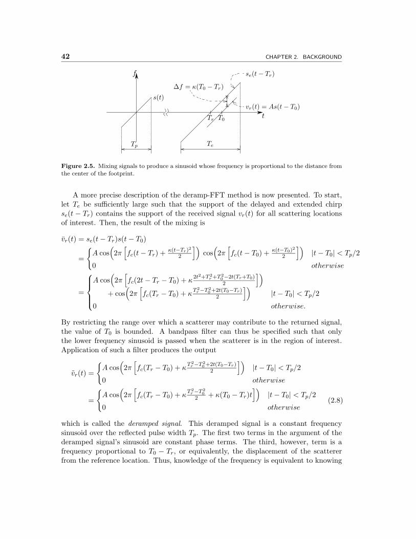
42 CHAPTER 2. BACKGROUND
f
tTr T0
s(t)
Tp Te
∆f = κ(T0 − Tr)
se(t− Tr)
vr(t) = As(t− T0)
Figure 2.5. Mixing signals to produce a sinusoid whose frequency is proportional to the distance fromthe center of the footprint.
A more precise description of the deramp-FFT method is now presented. To start,let Te be sufficiently large such that the support of the delayed and extended chirpse(t − Tr) contains the support of the received signal vr(t) for all scattering locationsof interest. Then, the result of the mixing is
vr(t) = se(t− Tr)s(t− T0)
=
{A cos
(2π[fc(t− Tr) +
κ(t−Tr)2
2
])cos
(2π[fc(t− T0) +
κ(t−T0)2
2
])|t− T0| < Tp/2
0 otherwise
=
A cos
(2π[fc(2t− Tr − T0) + κ
2t2+T 2r +T 2
0 −2t(Tr+T0)2
])+ cos
(2π[fc(Tr − T0) + κ
T 2r −T 2
0+2t(T0−Tr)2
])|t− T0| < Tp/2
0 otherwise.
By restricting the range over which a scatterer may contribute to the returned signal,the value of T0 is bounded. A bandpass filter can thus be specified such that onlythe lower frequency sinusoid is passed when the scatterer is in the region of interest.Application of such a filter produces the output
vr(t) =
{A cos
(2π[fc(Tr − T0) + κ
T 2r −T 2
0+2t(T0−Tr)2
])|t− T0| < Tp/2
0 otherwise
=
{A cos
(2π[fc(Tr − T0) + κ
T 2r −T 2
02 + κ(T0 − Tr)t
])|t− T0| < Tp/2
0 otherwise(2.8)
which is called the deramped signal. This deramped signal is a constant frequencysinusoid over the reflected pulse width Tp. The first two terms in the argument of thederamped signal’s sinusoid are constant phase terms. The third, however, term is afrequency proportional to T0 − Tr, or equivalently, the displacement of the scattererfrom the reference location. Thus, knowledge of the frequency is equivalent to knowing
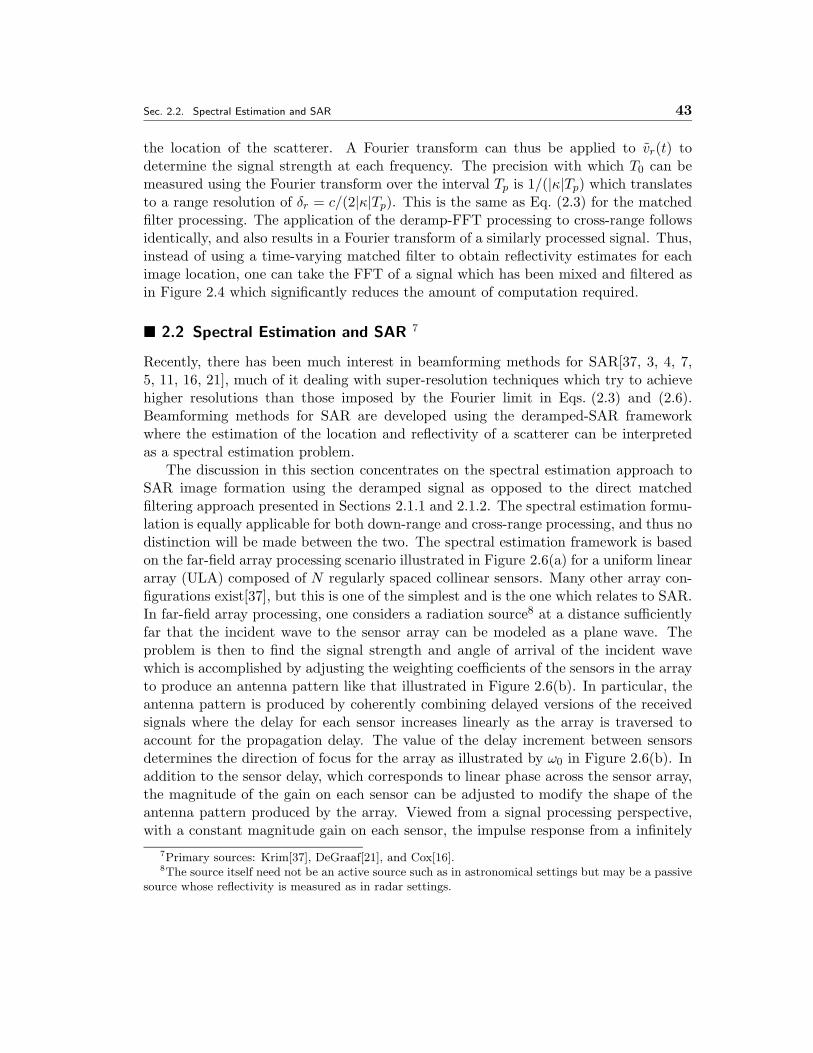
Sec. 2.2. Spectral Estimation and SAR 43
the location of the scatterer. A Fourier transform can thus be applied to vr(t) todetermine the signal strength at each frequency. The precision with which T0 can bemeasured using the Fourier transform over the interval Tp is 1/(|κ|Tp) which translatesto a range resolution of δr = c/(2|κ|Tp). This is the same as Eq. (2.3) for the matchedfilter processing. The application of the deramp-FFT processing to cross-range followsidentically, and also results in a Fourier transform of a similarly processed signal. Thus,instead of using a time-varying matched filter to obtain reflectivity estimates for eachimage location, one can take the FFT of a signal which has been mixed and filtered asin Figure 2.4 which significantly reduces the amount of computation required.
� 2.2 Spectral Estimation and SAR 7
Recently, there has been much interest in beamforming methods for SAR[37, 3, 4, 7,5, 11, 16, 21], much of it dealing with super-resolution techniques which try to achievehigher resolutions than those imposed by the Fourier limit in Eqs. (2.3) and (2.6).Beamforming methods for SAR are developed using the deramped-SAR frameworkwhere the estimation of the location and reflectivity of a scatterer can be interpretedas a spectral estimation problem.
The discussion in this section concentrates on the spectral estimation approach toSAR image formation using the deramped signal as opposed to the direct matchedfiltering approach presented in Sections 2.1.1 and 2.1.2. The spectral estimation formu-lation is equally applicable for both down-range and cross-range processing, and thus nodistinction will be made between the two. The spectral estimation framework is basedon the far-field array processing scenario illustrated in Figure 2.6(a) for a uniform lineararray (ULA) composed of N regularly spaced collinear sensors. Many other array con-figurations exist[37], but this is one of the simplest and is the one which relates to SAR.In far-field array processing, one considers a radiation source8 at a distance sufficientlyfar that the incident wave to the sensor array can be modeled as a plane wave. Theproblem is then to find the signal strength and angle of arrival of the incident wavewhich is accomplished by adjusting the weighting coefficients of the sensors in the arrayto produce an antenna pattern like that illustrated in Figure 2.6(b). In particular, theantenna pattern is produced by coherently combining delayed versions of the receivedsignals where the delay for each sensor increases linearly as the array is traversed toaccount for the propagation delay. The value of the delay increment between sensorsdetermines the direction of focus for the array as illustrated by ω0 in Figure 2.6(b). Inaddition to the sensor delay, which corresponds to linear phase across the sensor array,the magnitude of the gain on each sensor can be adjusted to modify the shape of theantenna pattern produced by the array. Viewed from a signal processing perspective,with a constant magnitude gain on each sensor, the impulse response from a infinitely
7Primary sources: Krim[37], DeGraaf[21], and Cox[16].8The source itself need not be an active source such as in astronomical settings but may be a passive
source whose reflectivity is measured as in radar settings.
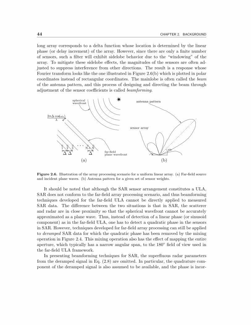
44 CHAPTER 2. BACKGROUND
long array corresponds to a delta function whose location is determined by the linearphase (or delay increment) of the array. However, since there are only a finite numberof sensors, such a filter will exhibit sidelobe behavior due to the “windowing” of thearray. To mitigate these sidelobe effects, the magnitudes of the sensors are often ad-justed to suppress interference from other directions. The result is a response whoseFourier transform looks like the one illustrated in Figure 2.6(b) which is plotted in polarcoordinates instead of rectangular coordinates. The mainlobe is often called the beamof the antenna pattern, and this process of designing and directing the beam throughadjustment of the sensor coefficients is called beamforming.
. ..1 2 3 N-1
∆ ∆ ∆N
wavefrontspherical
far-fieldplane wavefront
2π∆ cos(ω0)λ
sensor array
antenna pattern
ω0
(a) (b)
Figure 2.6. Illustration of the array processing scenario for a uniform linear array. (a) Far-field sourceand incident plane waves. (b) Antenna pattern for a given set of sensor weights.
It should be noted that although the SAR sensor arrangement constitutes a ULA,SAR does not conform to the far-field array processing scenario, and thus beamformingtechniques developed for the far-field ULA cannot be directly applied to measuredSAR data. The difference between the two situations is that in SAR, the scattererand radar are in close proximity so that the spherical wavefront cannot be accuratelyapproximated as a plane wave. Thus, instead of detection of a linear phase (or sinusoidcomponent) as in the far-field ULA, one has to detect a quadratic phase in the sensorsin SAR. However, techniques developed for far-field array processing can still be appliedto deramped SAR data for which the quadratic phase has been removed by the mixingoperation in Figure 2.4. This mixing operation also has the effect of mapping the entireaperture, which typically has a narrow angular span, to the 180◦ field of view used inthe far-field ULA framework.
In presenting beamforming techniques for SAR, the superfluous radar parametersfrom the deramped signal in Eq. (2.8) are omitted. In particular, the quadrature com-ponent of the deramped signal is also assumed to be available, and the phase is incor-
Sec. 2.2. Spectral Estimation and SAR 45
porated into the now complex reflectivity to write the simplified signal as
x(t) = A0ejω0t + n(t) (2.9)
where ω0 is the unknown frequency to be estimated (conveying scatterer location), A0
is the reflective gain from the scatterer, and n(t) is zero-mean circularly complex whiteGaussian noise with variance 2σ2 which represents the response from clutter in thetarget field. As the measurements are taken at discrete time samples (t1, t2, . . . , tN ),bold face letters are used to denote collections of sampled quantities, e.g. x denotesthe vector of all samples of x(t). Since the received data x is a random vector, ithas an associated correlation matrix which is denoted as R. The normalized modeledresponse for a scatterer corresponding to frequency ω0 is termed the steering vector andis denoted by a(ω0). In particular, the steering vector for an ideal point scatterer withassociated frequency ω0 is
a(ω0) =[ejω0t0 , ejω0t1 , ejω0t2 , . . .
]. (2.10)
This allows the samples of x(t) to be written as
x = A0a(ω0) + n
for the case of a single scatterer. For the multiple scatterer case, the received signal canbe written as
x =M∑
m=1
Ama(ωm) + n (2.11)
where M is the number of scatterers.The design objective in beamforming is to generate a highly directive gain peak
(or beam) and steer it to the desired location through adjustment of the weightingcoefficients. These coefficients are commonly taken as the solution to an optimizationproblem for a linear filter. Letting h∗(ω) denote the set of sensor weights applied to xto estimate the energy at frequency w, the output y(ω) is defined as
y(ω) � hH(ω)x.
A frequently used quantity which is useful in defining optimal filters is the power of theoutput y(ω)
P (y(ω)) � E[|y(ω)|2]
= hH(ω) E[xxH
]h(ω)
= hH(ω)Rh(ω).
Using these entities, there are many different beamformers that one could design. Inthe following sub-sections, two of the more popular ones are discussed.
46 CHAPTER 2. BACKGROUND
� 2.2.1 Conventional Beamformer
The first filter described is the conventional beamformer. This is motivated by the ideathat one wants to maximize the SNR of the filter output. In particular, we seek thefilter with unity energy which maximizes the output energy, i.e.
arg maxh(ω):‖h(ω)‖2=1
{P (y(ω))} = arg maxh(ω):‖h(ω)‖2=1
{E[hH(ω)xxHh(ω)
]}= arg max
h(ω):‖h(ω)‖2=1
{|A0|2hH(ω)aaHh(ω) + 2σ2h(ω)Hh(ω)}
= arg maxh(ω):‖h(ω)‖2=1
{hH(ω)aaHh(ω)
}. (2.12)
The solution for this maximization problem is
hconv(ω) =a(ω)√
a(ω)Ha(ω). (2.13)
Because this filter maximizes the SNR of the output, it is an implementation of thematched filter. Furthermore, because a(ω) is an exponential of frequency w, the outputhH(ω)x corresponds to a Fourier coefficient of x, and the collection of outputs over allw corresponds to the Fourier transform of x. This formulation supports the reasoningfor taking the Fourier transform of vr(t) at the end of Section 2.1.3 as it implements anapproximation of the matched filter9.
� 2.2.2 Capon’s Beamformer
The ideas for reflectivity estimation presented thus-far only consider the situation inwhich there is a single point scatterer. Super-resolution techniques, however, take intoaccount the presence of other dominant scatterers to suppress interference and betterresolve closely spaced sinusoids. Because the conventional beamformer is only concernedwith the estimation of a single scatter, it is not a super-resolution technique. Thissub-section describes Capon’s method which is a popular super-resolution techniquethat tries to suppress the effects of nearby interfering scatterers to achieve a higherresolution. In particular, Capon’s method determines the filter for each frequency ω asthe solution to the following optimization problem
argminh(ω)
{P (y(ω))}
s.t. hH(ω)a(ω) = 1. (2.14)
The idea here is to choose the filter which minimizes the total energy received whilehaving unity gain for the frequency ω. Thus, interference from nearby strong scatterersis suppressed as the resulting filter attempts place nulls at locations producing high
9From the formulation in Eq. (2.11), this is exactly the matched filter and not just an approximation,but recall that several approximations were made in Section 2.1.3 to formulate SAR into this model.

Sec. 2.3. Nonideal Scattering 47
energy contributions. Using standard optimization techniques, the solution for Capon’sbeamformer is
hCapon(ω) =R−1a(ω)
aH(ω)R−1a(ω). (2.15)
Note that this filter makes use of the received data via R to detect and null interferingscatterers. Thus, one cannot simply take R = 2σ2I as that would ignore the data andsimplify to the conventional beamformer. In array processing, R is typically estimatedfrom the received data as the sample correlation matrix of the sensor data. In SARhowever, this poses a problem since there is only one sample of the sensor data, i.e. theone image, which results in a correlation matrix with rank one. Typically, this obstacleis bypassed by using the assumption that the sensor domain data are stationary, andthus the sensors can be divided into multiple groups where each group can be treatedas a distinct sample of data[3, 37]. For more information on Capon’s methods and itsvariants, including applications to real SAR data, the reader is referred to [16, 4, 7, 5].
� 2.3 Nonideal Scattering 10
All the discussion up to this point has been based on the ideal point scattering model,i.e. scattering which is frequency and aspect independent, resulting in the received sig-nal being modeled as a simple delay of the transmitted signal regardless of orientation.However, even the most simple scattering primitives (spheres, plates, dihedrals, trihe-drals, cylinders, cones, etc.), exhibit either frequency and/or aspect dependences. Thedegree to which these dependencies manifest themselves depends on the geometry andphysical dimensions of the object. Recently, there has been much interest in determin-ing and exploiting the nonideal scattering behavior of simple scatterers especially forthe purpose of target classification[5, 40, 45, 13, 46]. This interest is particularly strongin applications using high resolution wide-band and wide-aperture data where thesedependencies are more pronounced.
Accurate scattering response models for canonical scatterers can be obtained fromphysics-based models such as physical optics (PO)[48] or the geometric theory of diffrac-tion (GTD)[33, 48]. For specific scatterer geometries, these models provide a closed formapproximation for the response as a function of scatterer size and orientation. The POmodel is obtain from the solution of a ray-tracing model including the effects of off-specular responses. The GTD model extends the PO model by also accounting forsurface currents and edge effects. The two models are nominally the same except atnear tangent incident angles where the GTD model is significantly better. This thesis isprimarily concerned with gross level scattering behavior around the specular responsewhere the scatterer is strongly observable. In this regime, the simpler PO model issufficient and thus the GTD model is not discussed further. To provide an idea of thedifferent responses that scatterers produce, the PO model for some simple canonical
10Primary sources: Ruck[48], Benitz[5], and Chaney[12].
48 CHAPTER 2. BACKGROUND
scatterers are cited from Ruck[48]. The first is the rectangular flat plate illustrated inFigure 2.7(a) where a flat plate of size a × b is centered at the origin and the radarbackscatter is measured from the direction given by φ and θ. For this configuration,the radar cross section11 (RCS) is given by
σ =4π(ab)2
λ2
[sin(θ)
sin(ka cos(θ) cos(φ))ka cos(θ) cos(φ)
sin(kb cos(θ) sin(φ))kb cos(θ) sin(φ)
]2(2.16)
where λ = c/f is the wavelength, k = 2πλ is the wavenumber, c is the speed of light,and f is the frequency of the signal. This response is plotted for a 1m×1m plate withf = 9.6GHz12, φ = 0◦, and θ ∈ [−30◦, 30◦]13 in Figure 2.8(a). The PO model for asphere of radius a centered at the origin as illustrated in Figure 2.7(b) is
σ = πa2[1− sin(2ka)
ka2− cos(2ka)
2k2a2
](2.17)
The azimuthal response for a = 1m is shown in Figure 2.8(b). Another canonicalscatterer is the right circular cylinder with radius a and height h centered at the originas illustrated in Figure 2.7(c). The PO response for this scatterer is
σ = kah2[cos(2θ)
sin(kh sin(2θ))kh sin(2θ)
]2(2.18)
which is plotted in Figure 2.8(c) for a =0.5m and h =1m with φ = 0◦. Figure 2.7(d)illustrates the dihedral canonical scatterer composed of two rectangular plates of sizea× b conjoined at the edge of length b such that the two plates form a 90◦ angle. ThePO response for this scatterer scatterer is
σ = π
[4abλ
cos(θ) sin(φ)sin(kb sin(θ))kb sin(θ)
]2. (2.19)
This response is plotted in Figure 2.8(d) for a =0.5m and b =1m when θ = 0◦.Given canonical scatterer models, a natural inclination is to use them to improve
reflectivity estimates. Extending the matched filtering approach in Sections 2.1.1 and2.1.2 to handle nonideal scattering would be quite difficult both analytically and com-putationally. However, nonideal scattering could be incorporated by using the predictedresponse in place of the point-scatterer steering vector in Eq. (2.10) in the beamformerspresented earlier. The general solution for the conventional beamformer in Eq. (2.13)and Capon’s beamformer in Eq. (2.15) still hold under these more general steeringvectors. Benitz [7, 5] takes such an approach in his high-definition vector imaging
11RCS is a measure of the reflected power.12This is the same as the MSTAR center frequency (see Appendix B).13Such a large azimuthal range is used for illustrative purposes and is beyond the capabilities of
current SAR systems. Typical azimuthal spans in modern systems are as low as 1◦ and as high as 30◦.Furthermore, the PO approximations start to lose their accuracy beyond the displayed range.
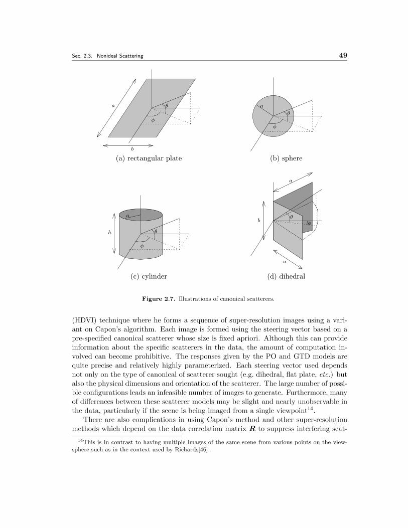
Sec. 2.3. Nonideal Scattering 49
φ
a
b
θ
θ
a
φ
(a) rectangular plate (b) sphere
φ
θ
a
h
θφ
a
b
a
(c) cylinder (d) dihedral
Figure 2.7. Illustrations of canonical scatterers.
(HDVI) technique where he forms a sequence of super-resolution images using a vari-ant on Capon’s algorithm. Each image is formed using the steering vector based on apre-specified canonical scatterer whose size is fixed apriori. Although this can provideinformation about the specific scatterers in the data, the amount of computation in-volved can become prohibitive. The responses given by the PO and GTD models arequite precise and relatively highly parameterized. Each steering vector used dependsnot only on the type of canonical of scatterer sought (e.g. dihedral, flat plate, etc.) butalso the physical dimensions and orientation of the scatterer. The large number of possi-ble configurations leads an infeasible number of images to generate. Furthermore, manyof differences between these scatterer models may be slight and nearly unobservable inthe data, particularly if the scene is being imaged from a single viewpoint14.
There are also complications in using Capon’s method and other super-resolutionmethods which depend on the data correlation matrix R to suppress interfering scat-
14This is in contrast to having multiple images of the same scene from various points on the view-sphere such as in the context used by Richards[46].
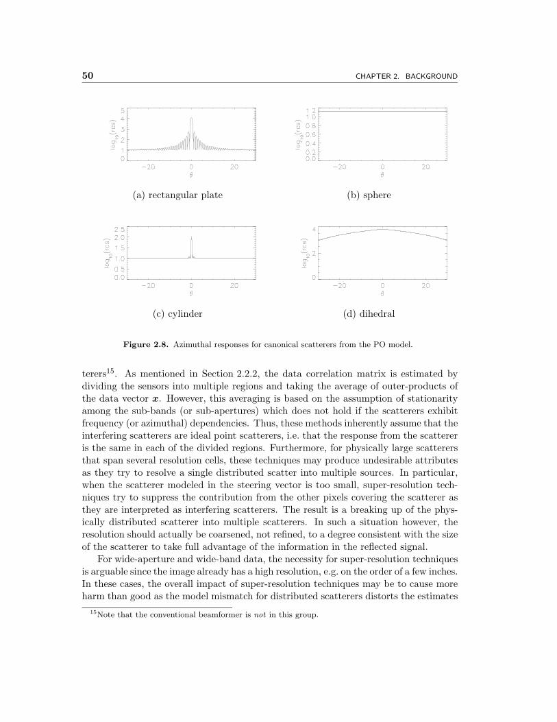
50 CHAPTER 2. BACKGROUND
(a) rectangular plate (b) sphere
(c) cylinder (d) dihedral
Figure 2.8. Azimuthal responses for canonical scatterers from the PO model.
terers15. As mentioned in Section 2.2.2, the data correlation matrix is estimated bydividing the sensors into multiple regions and taking the average of outer-products ofthe data vector x. However, this averaging is based on the assumption of stationarityamong the sub-bands (or sub-apertures) which does not hold if the scatterers exhibitfrequency (or azimuthal) dependencies. Thus, these methods inherently assume that theinterfering scatterers are ideal point scatterers, i.e. that the response from the scattereris the same in each of the divided regions. Furthermore, for physically large scatterersthat span several resolution cells, these techniques may produce undesirable attributesas they try to resolve a single distributed scatter into multiple sources. In particular,when the scatterer modeled in the steering vector is too small, super-resolution tech-niques try to suppress the contribution from the other pixels covering the scatterer asthey are interpreted as interfering scatterers. The result is a breaking up of the phys-ically distributed scatterer into multiple scatterers. In such a situation however, theresolution should actually be coarsened, not refined, to a degree consistent with the sizeof the scatterer to take full advantage of the information in the reflected signal.
For wide-aperture and wide-band data, the necessity for super-resolution techniquesis arguable since the image already has a high resolution, e.g. on the order of a few inches.In these cases, the overall impact of super-resolution techniques may be to cause moreharm than good as the model mismatch for distributed scatterers distorts the estimates
15Note that the conventional beamformer is not in this group.
Sec. 2.3. Nonideal Scattering 51
as larger scatterers are broken into smaller scatterers. Rather than forming myriad esti-mates based on a large assortment of canonical scatterer types, sizes, and orientations,it is reasonable to take a more general but physically meaningful characterization of thescattering response. This is the approach taken by Chaney et. al.[12] who propose tomodel scatterer anisotropy in a coarse manner capturing the fact that for many scatter-ers, anisotropy is related to their physical size. To simplify the amount of computation,they approximate the aspect dependent scattering as zero from all azimuthal directionsexcept over a section of the aperture where the gain is constant, i.e.
a(ω) =
{A0 ω1 ≤ ω ≤ ω2
0 o.w.
for some ω1 and ω2. The matched filter in azimuth is then a windowed FFT (in thebeamforming framework) and is equivalent to processing with just a subset of the full-aperture. The weighting across the sub-aperture is uniform as in the point scatterercase and is not exactly tuned to any particular scatterer. Although, this implies thatoptimal processing is not performed, myriad images need not be generated for all thescattering types sought and general differences in scatterer anisotropy can be detected.Chaney et. al. utilize sub-aperture processing by adapting the size and location ofthe sub-aperture to achieve a better reflectivity estimate for anisotropic scatterers.For example, the broadside flash phenomena associated with a large plate producesa scattering response which is concentrated in a small section of the aperture. Thus,by only using the section of the aperture in which most of the returned energy isconcentrated, a higher fidelity estimate of the reflectivity can be achieved since onlythe portion with a high SNR is used. Viewed in the image domain rather than thesensor domain, this can be interpreted as adjusting the amount of spatial coarseningbased on the spatial extent of the scatterer. For each pixel in their algorithm, theycompute a set of reflectivity estimates from various sub-apertures and choose the onewith the highest reflectivity. The resulting image is then thresholded to detect brightanisotropic scatterers. One drawback to this approach is that their selection criterionfor the sub-aperture is based on a model which does not properly take into account theeffect of sub-aperture length on the variance of the sub-aperture reflectivity estimate.The resulting images produced by their criterion have an excessively coarse resolutionimplying that too small an aperture is frequently used. Furthermore, Chaney onlyuses the reflectivity estimate and discards the properties of the chosen sub-aperture,i.e. its size and location. By ignoring these specifics, possible information about thescatterer’s size and orientation is lost. From the duration of the flash (in terms ofaperture length), the size of the scatterer can be inferred since scatterer size is inverselyproportional to the duration of the flash. From the center of the flash, the orientationof the scatterer can be inferred. For example, the peak response of a flat plate shouldoccur at broadside.
52 CHAPTER 2. BACKGROUND
� 2.4 Machine Learning
The field of machine learning deals with the use of computers to “learn” patterns inthe data and make decisions based upon the knowledge gained. This thesis is con-cerned with the classification subset of machine learning. Obviously, knowledge of theunderlying probability distribution of the classes involved is fundamental to any goodprobabilistic algorithm. However, these distributions are not known and must be esti-mated. Another issue is how to use these estimated distributions. This section presentsthe relevant background needed to address these problems. First, the topic of densityestimation is discussed. This is followed by a presentation of some fundamental conceptsin information theory. These concepts are then used to show the asymptotic equivalencebetween the likelihood ratio and the information theoretic concept of Kullback-Leibler(KL) divergence. Finally, a classification approach comparing estimated densities viaKL divergence is presented.
� 2.4.1 Kernel Based Density Estimation 16
Knowledge of probability densities is essential in the field of stochastic signal processing.Thus, the relevant densities must be estimated to some degree. Some tasks require onlya few statistics whereas others require the entire pdf, and the former often make strongassumptions about the underlying density. Techniques for density estimation broadlyfall into one of two categories. The first is called parametric estimation. In this case, aparticular parametric form for the density is assumed and its parameters are estimatedfrom data. For example, one may assume the underlying density is a Gaussian and usethe data to estimate its mean and covariance. The limitations of such parametric tech-niques are clear in that the functional form assumed imposes a strong restriction. Theclass of nonparametric density estimators make few assumptions on the density (such asregularity) and lets the number of parameters describing the density grow unboundedwith the amount of data. It is often advantageous to use a nonparametric estimatorwhen little is known about the underlying phenomena producing the sample values,and thus, one has no reason to assume a particular family of density functions. Forexample, visually viewing a nonparametric estimate of the density (e.g. a histogram) isoften a useful first step in choosing one or more functionals to describe the data andpossibly associate underlying causes with different parts of the distribution. However,the wealth of unlimited choices for the density makes this an ill-posed estimation prob-lem. Even when a particular degree of regularity is assumed, estimation is difficult inregions where only a few local samples are available.
Before describing a common technique for density estimation, some notation mustbe defined. Lowercase boldface letters are used to denote random vectors, e.g. x, andsamples of it are denoted with a corresponding uppercase letter, e.g. X. Calligraphicletters, e.g. X , are used to denote the corresponding sample space. The distribution for
16Primary sources: Silverman[50] and Fukunaga[26].
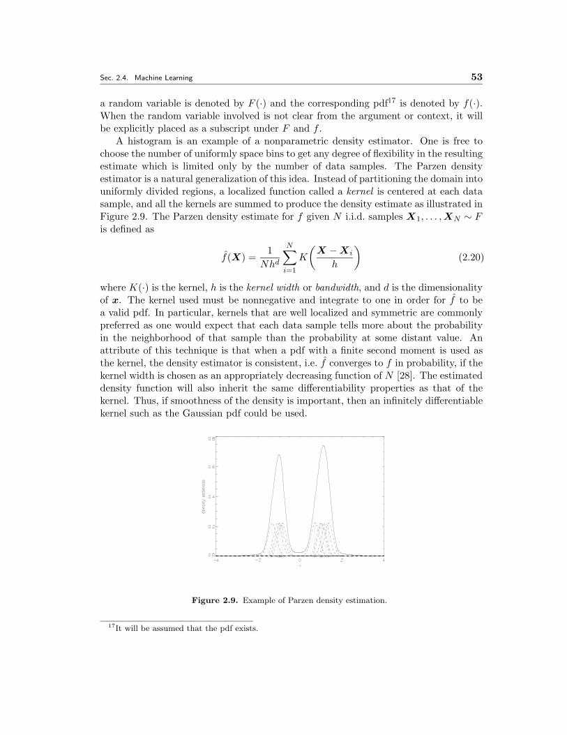
Sec. 2.4. Machine Learning 53
a random variable is denoted by F (·) and the corresponding pdf17 is denoted by f(·).When the random variable involved is not clear from the argument or context, it willbe explicitly placed as a subscript under F and f .
A histogram is an example of a nonparametric density estimator. One is free tochoose the number of uniformly space bins to get any degree of flexibility in the resultingestimate which is limited only by the number of data samples. The Parzen densityestimator is a natural generalization of this idea. Instead of partitioning the domain intouniformly divided regions, a localized function called a kernel is centered at each datasample, and all the kernels are summed to produce the density estimate as illustrated inFigure 2.9. The Parzen density estimate for f given N i.i.d. samples X1, . . . ,XN ∼ Fis defined as
f(X) =1
Nhd
N∑i=1
K
(X −Xi
h
)(2.20)
where K(·) is the kernel, h is the kernel width or bandwidth, and d is the dimensionalityof x. The kernel used must be nonnegative and integrate to one in order for f to bea valid pdf. In particular, kernels that are well localized and symmetric are commonlypreferred as one would expect that each data sample tells more about the probabilityin the neighborhood of that sample than the probability at some distant value. Anattribute of this technique is that when a pdf with a finite second moment is used asthe kernel, the density estimator is consistent, i.e. f converges to f in probability, if thekernel width is chosen as an appropriately decreasing function of N [28]. The estimateddensity function will also inherit the same differentiability properties as that of thekernel. Thus, if smoothness of the density is important, then an infinitely differentiablekernel such as the Gaussian pdf could be used.
Figure 2.9. Example of Parzen density estimation.
17It will be assumed that the pdf exists.
54 CHAPTER 2. BACKGROUND
� 2.4.2 Information and Entropy 18
Although the ideas in information theory originated in the communications field, theapplication of its results extend far into many other fields. The central ideas in in-formation theory regard how much “information” is present in a sequence of randomvariables and how efficiently that sequence can be coded, where efficiency is measuredin terms of the size of the coded sequence and robustness to noise. Intuitively, this isanalogous to the idea of classification by which this thesis is motivated. The object tobe identified can be considered the “information” in the signal; the coded sequence canbe thought of as the features used to identify the object; the distortions in the imagedata along with the data lost due to projecting onto the feature set can be thought ofas the noise in the communications channel. The goal in ATR is to choose the bestfeature set (code) that efficiently conveys the object’s identity (information), but whichis robust to imaging noise and data not captured by the feature set (channel noise).In this section, a basic review of some fundamental information theoretic concepts arepresented.
First, the concept of quantifying information is considered. Given an event E thatoccurs with probability p, we wish to quantify the amount of surprise S(p) in learningthat E has occurred. It can be shown that if the surprise satisfies the following fouraxioms, then it has the form
S(p) = −c log(p)
where the constant c is an arbitrary positive integer, taken to be 1, and the base of thelogarithm is arbitrary, generally taken to be 2. The four axioms are
• Axiom 1: S(1) = 0. That is, there is no surprise in observing a sure event.
• Axiom 2: S(p) is a strictly decreasing function of p. That is, the occurrence ofless likely events generate more surprise.
• Axiom 3: S(p) is a continuous function of p. That is, small changes in theprobability of an event correspond to small changes in the surprise of observingthat event.
• Axiom 4: S(pq) = S(p) + S(q), where q is the probability of an event F indepen-dent of E. That is, the surprise of observing two independent events is the sumof their surprises.
Now, consider a discrete random variable y that can take on values Y ∈ Y withprobabilities p(Y ). The entropy of y is defined as the expected value of the surprise ofthe outcome, i.e.
H(y) = E[− log(p(y))] = −∑Y ∈Y
p(Y ) log(p(Y )) . (2.21)
18Primary sources: Cover[15] and Ross[47].
Sec. 2.4. Machine Learning 55
As its name implies, entropy is a measure of randomness of the outcomes of the randomvariable. Extending this idea of entropy to continuous random variables, the differentialentropy of a random variable distributed according to the pdf f is defined as
h(x) = E[− log(f(x))] = −∫X
log(f(X)) dF (X) . (2.22)
Another useful concept from information theory useful for ATR is the continuousform of the Kullback-Leibler (KL) divergence between two pdf’s f and g. The KLdivergence is defined as
D(f‖g) =∫
f(X) log(f(X)g(X)
)dX (2.23)
which is the expected value, under f , of the log-likelihood ratio of f and g.19 It is usefulto think of the KL divergence as a distance between two pdf’s, even though it does notqualify as a metric since neither the symmetry condition nor the triangle inequalityhold. One property of metrics that it does possess is that the KL divergence betweentwo pdf’s is always nonnegative and it is zero if and only if the two pdf’s are equal.
Another useful property of the KL divergence is its relation to the log-likelihood ratio(LLR). This relationship is attractive because a thresholding of the LLR, i.e. a likelihoodratio test (LRT), is the optimal20 decision rule for a hypothesis test. In particular, thehypothesis test considered is: given a sequence of samples {X1, . . . ,XN}, we wish tochoose one of two hypotheses to describe the nature of the samples
H1 : xi i.i.d. ∼ f = f1 orH2 : xi i.i.d. ∼ f = f2.
where f is the density producing the samples and f1 and f2 are two specified hypothesisdensities. It is relatively straightforward to show that
Ef
[log(f1(x)f2(x)
)]= D(f‖f2)−D(f‖f1), (2.24)
i.e. the differences between KL divergences in Eq. (2.24) is the expected value of theLLR. This equivalence motivates the classification approach discussed in the next sub-section which uses the KL divergence between densities, estimated from samples, as thebasis for a decision rule.
� 2.4.3 KL-Based Classification Technique 21
To conclude the section on machine learning, several of the machine learning compo-nents presented are used to describe a classifier which asymptotically approaches the
19For continuity, 0 log(
00
)is defined to be 0.
20The LRT is optimal in the sense that for a specified cost structure on the different classificationdecisions under the true hypothesis, the rule which minimizes the expected cost is an LRT.
21This section is a generalization of the approach described by DeBonet[20] whose specifics are de-scribed in Appendix A.
56 CHAPTER 2. BACKGROUND
likelihood ratio test without assuming parametric forms for any of the underlying data.The setup for the problem is as follows. The learning process is based on L labeled sets{S1, . . . ,SL} of reference data each containing N samples. For each l, all the samples inSl are generated as i.i.d. samples from the labeled but unknown density fl. Then, pre-sented with another set S0 = {X1, . . . ,XN} of data consisting of i.i.d. samples drawnfrom one of the densities fl, the problem is to choose under which fl the samples of S0were generated.
The first task in this approach is to compute fl, the density estimate for fl, foreach l ∈ {0, . . . , L}. Because no parametric forms of the densities are to be assumed,a consistent nonparametric density estimator22, such as the Parzen density estimator,should be used.
Motivated by the equivalence of the expected value of the LLR and KL divergencein Eq. (2.24), the following derivation shows that the minimization of KL divergencesis asymptotically equivalent to maximum likelihood testing for the problem defined atthe beginning of the section. Starting from the maximum likelihood (ML) detector forthe density generating the data set S0:
l = arg maxl∈{1,...,L}
{fl(X1, . . . ,XN )}
= argmaxl
{N∏i=1
fl(Xi)
}
≈ argmaxl
{N∏i=1
fl(Xi)
}
= argmaxl
{N∏i=1
fl(Xi)
f0(Xi)f0(Xi)
}
= argmaxl
{N∏i=1
fl(Xi)
f0(Xi)
}
= argmaxl
{N∑i=1
log
(fl(Xi)
f0(Xi)
)}
= argminl
{1N
N∑i=1
log
(f0(Xi)
fl(Xi)
)}
≈ argminl
{∫f0(X) log
(f0(X)
fl(X)
)dX
}= argmin
l
{D(f0‖fl)
}. (2.25)
22For other consistent density estimators, the reader is referred to Silverman[50].
Sec. 2.4. Machine Learning 57
All approximations in Eq. (2.25) are meant in the sense that the argument of theargmax {·} is approximate. The first approximation, based on the consistency of thedensity estimator, is that the estimated pdf’s are close to the true underlying pdf’s.The second approximation is that the relative frequency of each X ∈ X converges23 tothe estimated probability f0(X). The result in Eq. (2.25) thus says that the choosingthe fl which is “closest” to f0 in terms of the KL divergence is asymptotically equivalentto performing ML detection. Furthermore, if a rejection hypothesis is incorporated via
l =
{l∗ � argminl
{D(f0‖fl)
}D(f0‖fl∗) ≤ T
none of the available hypothesis are true D(f0‖fl∗) > T(2.26)
for a threshold T , then this decision rule is asymptotically equivalent to selecting thepdf which minimizes the KL divergence only if
Ef0
[log(fl(x)
)]> T
i.e. the estimated log-likelihood is greater than T .
23There are actually two asymptotic results being used here. Both the relative frequency of occurrencein S0 and the density estimate converge in probability to the true pdf and thus to each other. Theformer is by the weak law of large numbers, and the latter is by consistency of the density estimator.

58 CHAPTER 2. BACKGROUND
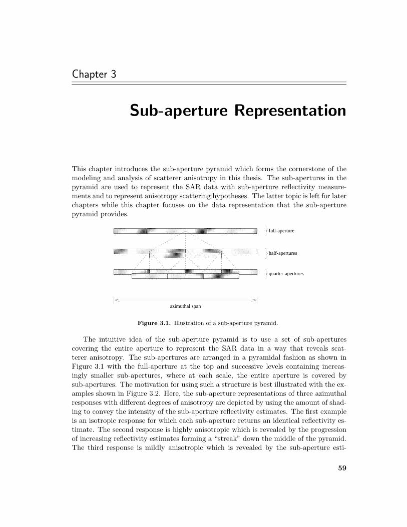
Chapter 3
Sub-aperture Representation
This chapter introduces the sub-aperture pyramid which forms the cornerstone of themodeling and analysis of scatterer anisotropy in this thesis. The sub-apertures in thepyramid are used to represent the SAR data with sub-aperture reflectivity measure-ments and to represent anisotropy scattering hypotheses. The latter topic is left for laterchapters while this chapter focuses on the data representation that the sub-aperturepyramid provides.
������������������������������������������������������������������������
����������������������������������������
����������������������������������������
����������������������������������������������������������������������������
������������������������������������������������������������������������������������������������������������������������������������������������
������������������������������������
������������������������������������
������������������������������������
������������������������������������
����������������������������������������
������������������������������������������������������������������������
azimuthal span
full-aperture
quarter-apertures
half-apertures
Figure 3.1. Illustration of a sub-aperture pyramid.
The intuitive idea of the sub-aperture pyramid is to use a set of sub-aperturescovering the entire aperture to represent the SAR data in a way that reveals scat-terer anisotropy. The sub-apertures are arranged in a pyramidal fashion as shown inFigure 3.1 with the full-aperture at the top and successive levels containing increas-ingly smaller sub-apertures, where at each scale, the entire aperture is covered bysub-apertures. The motivation for using such a structure is best illustrated with the ex-amples shown in Figure 3.2. Here, the sub-aperture representations of three azimuthalresponses with different degrees of anisotropy are depicted by using the amount of shad-ing to convey the intensity of the sub-aperture reflectivity estimates. The first exampleis an isotropic response for which each sub-aperture returns an identical reflectivity es-timate. The second response is highly anisotropic which is revealed by the progressionof increasing reflectivity estimates forming a “streak” down the middle of the pyramid.The third response is mildly anisotropic which is revealed by the sub-aperture esti-
59
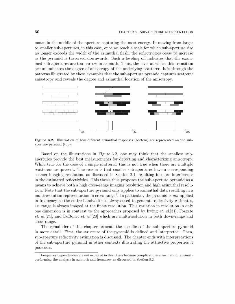
60 CHAPTER 3. SUB-APERTURE REPRESENTATION
mates in the middle of the aperture capturing the most energy. In moving from largerto smaller sub-apertures, in this case, once we reach a scale for which sub-aperture sizeno longer exceeds the width of the azimuthal flash, the reflectivities cease to increaseas the pyramid is traversed downwards. Such a leveling off indicates that the exam-ined sub-apertures are too narrow in azimuth. Thus, the level at which this transitionoccurs indicates the degree of anisotropy of the underlying scatterer. It is through thepatterns illustrated by these examples that the sub-aperture pyramid captures scattereranisotropy and reveals the degree and azimuthal location of the anisotropy.
az. az.az.
Figure 3.2. Illustration of how different azimuthal responses (bottom) are represented on the sub-aperture pyramid (top).
Based on the illustrations in Figure 3.2, one may think that the smallest sub-apertures provide the best measurements for detecting and characterizing anisotropy.While true for the case of a single scatterer, this is not true when there are multiplescatterers are present. The reason is that smaller sub-apertures have a correspondingcoarser imaging resolution, as discussed in Section 2.1, resulting in more interferencein the estimated reflectivities. This thesis thus proposes the sub-aperture pyramid as ameans to achieve both a high cross-range imaging resolution and high azimuthal resolu-tion. Note that the sub-aperture pyramid only applies to azimuthal data resulting in amultiresolution representation in cross-range1. In particular, the pyramid is not appliedin frequency as the entire bandwidth is always used to generate reflectivity estimates,i.e. range is always imaged at the finest resolution. This variation in resolution in onlyone dimension is in contrast to the approaches proposed by Irving et. al.[31], Fosgateet. al.[24], and DeBonet et. al.[20] which are multiresolution in both down-range andcross-range.
The remainder of this chapter presents the specifics of the sub-aperture pyramidin more detail. First, the structure of the pyramid is defined and interpreted. Then,sub-aperture reflectivity estimation is discussed. The chapter ends with interpretationsof the sub-aperture pyramid in other contexts illustrating the attractive properties itpossesses.
1Frequency dependencies are not explored in this thesis because complications arise in simultaneouslyperforming the analysis in azimuth and frequency as discussed in Section 8.2.
Sec. 3.1. Sub-aperture Pyramid 61
� 3.1 Sub-aperture Pyramid
Each sub-aperture can be associated with an interval of the real line. In particular, thefull-aperture is denoted by the interval [0, 1) = {t|0 ≤ t < 1}. Then, the sub-aperturecan be defined with simple set theoretic notions. The intuitive idea of the sub-aperturepyramid is to generate an over-complete covering of the full-aperture with sub-aperturesthat can be arranged in a pyramidal structure. Formally, the sub-aperture pyramid istaken to be a set S of sub-apertures with the following structure. The set S is partitionedinto smaller sets Sm for m ∈ {0, . . . ,M} all the elements of which have a particularsub-aperture length with larger values of m conveying smaller sub-aperture lengths asillustrated in Figure 3.3. S0 refers to the singleton set consisting of the full-aperture atthe top of the pyramid, and SM refers to the set of the smallest sub-apertures at thebottom of the pyramid. A second subscript on S denotes a specific sub-aperture at thegiven scale. For what follows later in the thesis, the following conditions are imposedon S:
(A) ∀Sm,i, Sm,i = [a, b) ⊂ [0, 1) for some a and b with 0 ≤ a < b ≤ 1,
(B) S0 = {[0, 1)},(C) ∀Sm,i,∃ a partition P(m, i) ⊂ SM of Sm,i, and
(D) ∀Sm,i with m ≥ 1, ∃Sm−1,j such that Sm,i ⊂ Sm−1,j .
The first condition simply restricts each sub-aperture to be a connected subset ofthe available aperture. The use of connected sets is motivated by the predominanceof concentrated unimodal scattering in azimuth produced by canonical scatterers. Thesecond condition states that the full-aperture resides at the top of the pyramid whichallows for consideration of the minimal degree of anisotropy, and more importantly,produces the finest imaging resolution permissible. The third condition ensures thateach sub-aperture can be represented by a partition of smallest-sized sub-apertures atthe bottom of the pyramid. This partitioning permits for simplified analysis in thesub-aperture attribution discussed in Chapter 5. The fourth condition asserts thateach sub-aperture, except the full-aperture, is contained within a parent sub-aperture.Herein, the term sub-aperture pyramid refers to one satisfying conditions (A)-(D).
To illustrate the idea of the sub-aperture pyramid, three examples are presented.The first is the disjoint, half-aperture pyramid shown in Figure 3.3(a). Here, each sub-aperture is divided into two halves for each change in scale thus producing a dyadicpartitioning of the aperture. At each scale, this pyramid uses the minimum number ofsub-apertures to achieve the covering for a given sub-aperture length. Such a minimalrepresentation, however, is not robust to shifts in the azimuthal response. For example,if the rightmost azimuthal response in Figure 3.2 were applied to the disjoint cover-ing, then the response could not be well captured with the set of half-apertures, andone would have to resort to using smaller sub-apertures which have a coarser imagingresolution. An approach to addressing to such a problem is to increase the amount
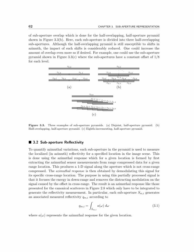
62 CHAPTER 3. SUB-APERTURE REPRESENTATION
of sub-aperture overlap which is done for the half-overlapping, half-aperture pyramidshown in Figure 3.3(b). Here, each sub-aperture is divided into three half-overlappingsub-apertures. Although the half-overlapping pyramid is still susceptible to shifts inazimuth, the impact of such shifts is considerably reduced. One could increase theamount of overlap even more so if desired. For example, one could use the sub-aperturepyramid shown in Figure 3.3(c) where the sub-apertures have a constant offset of 1/8for each level.
S2,0
S0,0
S1,0 S1,1
S2,1 S2,3S2,2 S2,0
S0,0
S1,0 S1,2
S1,1S2,2
S2,1 S2,3 S2,5
S2,6S2,4
(a) (b)
S0,0
S1,0 S1,1 S1,2 S1,3 S1,4
S2,0 S2,1 S2,4 S2,5 S2,6S2,2 S2,3
(c)
Figure 3.3. Three examples of sub-aperture pyramids. (a) Disjoint, half-aperture pyramid. (b)Half-overlapping, half-aperture pyramid. (c) Eighth-incrementing, half-aperture pyramid.
� 3.2 Sub-aperture Reflectivity
To quantify azimuthal variations, each sub-aperture in the pyramid is used to measurethe localized (in azimuth) reflectivity for a specified location in the image scene. Thisis done using the azimuthal response which for a given location is formed by firstextracting the azimuthal sensor measurements from range compressed data for a givenrange location. This produces a 1-D signal along the aperture which is not cross-rangecompressed. The azimuthal response is then obtained by demodulating this signal forits specific cross-range location. The purpose in using this partially processed signal isthat it focuses the energy in down-range and removes the distracting modulation on thesignal caused by the offset in cross-range. The result is an azimuthal response like thosepresented for the canonical scatterers in Figure 2.8 which only have to be integrated togenerate the reflectivity measurement. In particular, each sub-aperture Sm,i generatesan associated measured reflectivity qm,i according to
qm,i =∫Sm,i
a(ω) dω (3.1)
where a(ω) represents the azimuthal response for the given location.
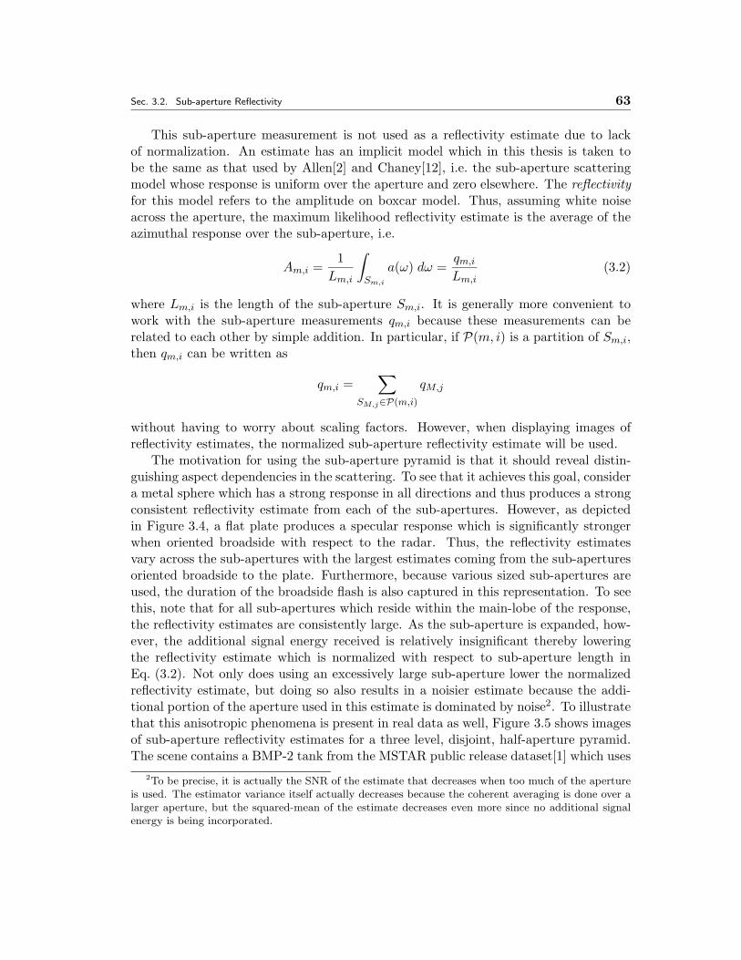
Sec. 3.2. Sub-aperture Reflectivity 63
This sub-aperture measurement is not used as a reflectivity estimate due to lackof normalization. An estimate has an implicit model which in this thesis is taken tobe the same as that used by Allen[2] and Chaney[12], i.e. the sub-aperture scatteringmodel whose response is uniform over the aperture and zero elsewhere. The reflectivityfor this model refers to the amplitude on boxcar model. Thus, assuming white noiseacross the aperture, the maximum likelihood reflectivity estimate is the average of theazimuthal response over the sub-aperture, i.e.
Am,i =1
Lm,i
∫Sm,i
a(ω) dω =qm,i
Lm,i(3.2)
where Lm,i is the length of the sub-aperture Sm,i. It is generally more convenient towork with the sub-aperture measurements qm,i because these measurements can berelated to each other by simple addition. In particular, if P(m, i) is a partition of Sm,i,then qm,i can be written as
qm,i =∑
SM,j∈P(m,i)
qM,j
without having to worry about scaling factors. However, when displaying images ofreflectivity estimates, the normalized sub-aperture reflectivity estimate will be used.
The motivation for using the sub-aperture pyramid is that it should reveal distin-guishing aspect dependencies in the scattering. To see that it achieves this goal, considera metal sphere which has a strong response in all directions and thus produces a strongconsistent reflectivity estimate from each of the sub-apertures. However, as depictedin Figure 3.4, a flat plate produces a specular response which is significantly strongerwhen oriented broadside with respect to the radar. Thus, the reflectivity estimatesvary across the sub-apertures with the largest estimates coming from the sub-aperturesoriented broadside to the plate. Furthermore, because various sized sub-apertures areused, the duration of the broadside flash is also captured in this representation. To seethis, note that for all sub-apertures which reside within the main-lobe of the response,the reflectivity estimates are consistently large. As the sub-aperture is expanded, how-ever, the additional signal energy received is relatively insignificant thereby loweringthe reflectivity estimate which is normalized with respect to sub-aperture length inEq. (3.2). Not only does using an excessively large sub-aperture lower the normalizedreflectivity estimate, but doing so also results in a noisier estimate because the addi-tional portion of the aperture used in this estimate is dominated by noise2. To illustratethat this anisotropic phenomena is present in real data as well, Figure 3.5 shows imagesof sub-aperture reflectivity estimates for a three level, disjoint, half-aperture pyramid.The scene contains a BMP-2 tank from the MSTAR public release dataset[1] which uses
2To be precise, it is actually the SNR of the estimate that decreases when too much of the apertureis used. The estimator variance itself actually decreases because the coherent averaging is done over alarger aperture, but the squared-mean of the estimate decreases even more since no additional signalenergy is being incorporated.
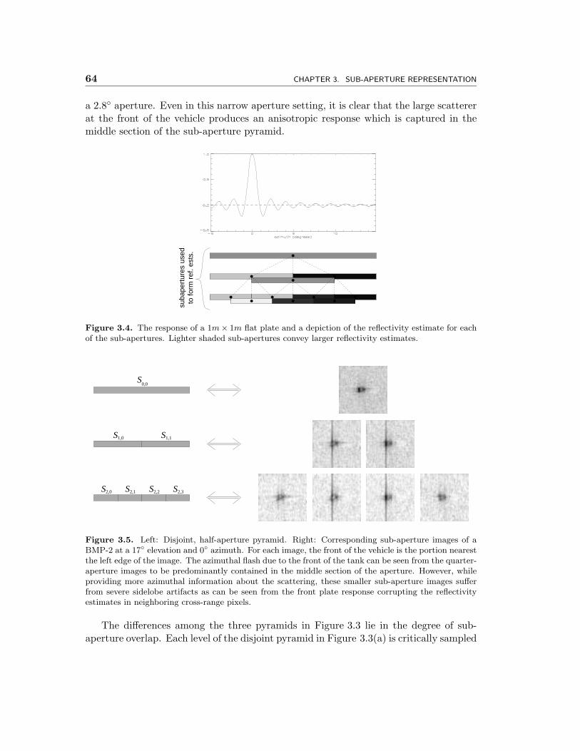
64 CHAPTER 3. SUB-APERTURE REPRESENTATION
a 2.8◦ aperture. Even in this narrow aperture setting, it is clear that the large scattererat the front of the vehicle produces an anisotropic response which is captured in themiddle section of the sub-aperture pyramid.
suba
pert
ures
use
dto
form
ref
. est
s.
Figure 3.4. The response of a 1m× 1m flat plate and a depiction of the reflectivity estimate for eachof the sub-apertures. Lighter shaded sub-apertures convey larger reflectivity estimates.
S0,0
2,0S 2,1S 2,2S 2,3S
1,0S 1,1S
Figure 3.5. Left: Disjoint, half-aperture pyramid. Right: Corresponding sub-aperture images of aBMP-2 at a 17◦ elevation and 0◦ azimuth. For each image, the front of the vehicle is the portion nearestthe left edge of the image. The azimuthal flash due to the front of the tank can be seen from the quarter-aperture images to be predominantly contained in the middle section of the aperture. However, whileproviding more azimuthal information about the scattering, these smaller sub-aperture images sufferfrom severe sidelobe artifacts as can be seen from the front plate response corrupting the reflectivityestimates in neighboring cross-range pixels.
The differences among the three pyramids in Figure 3.3 lie in the degree of sub-aperture overlap. Each level of the disjoint pyramid in Figure 3.3(a) is critically sampled
Sec. 3.3. Interpretations 65
in the sense that it has the minimal covering of the full-aperture. The other twopyramids are “oversampled” in azimuth as they populate the pyramid with additionaloverlapping sub-apertures that introduce no new information, although their presencemore clearly reveals the properties of “misaligned” azimuthal flashes which do notexactly line up with the divisions of the minimal disjoint pyramid representation. Thisexample illustrates the purpose of the redundant overlapping sub-apertures which is toprovide robustness to azimuthal shifts of the data, i.e. slight rotations of the target.The appropriate azimuthal oversampling for a pyramid is an open issue which involvesbalancing model approximation error and computational burden. The optimal trade-offbetween these two costs is an issue not addressed in this thesis. In our experiments,the half-overlapping, half-aperture pyramid works reasonably well and will be used forthe remainder of the thesis.
� 3.3 Interpretations
The sub-aperture pyramid is an over-complete representation of the SAR data. Thereason for this over-completeness is to aid the robust utilization of anisotropic scattering.To help the understanding of the sub-aperture pyramid, this section comments on therepresentation in the context of existing works.
� 3.3.1 Time-Frequency Plane Tilings
Because the integration in Eq. (3.2) is only performed over the sub-aperture Sm,i, thiscorresponds to a Fourier coefficient of windowed data. The use of smaller sub-aperturewindows thus produces estimates with a coarser imaging resolution. This trade-off isexactly the Fourier time-frequency uncertainty principle applied to SAR data, i.e. withpurely linearly processing, one cannot obtain both high azimuthal (time) and high cross-range (frequency) resolution due to the inverse relationship between the two. Thus,each level of the pyramid provides a different azimuthal–cross-range resolution trade-offwhich is best illustrated with the time-frequency plane tilings used in signal processingand wavelets in particular[59]. Each level of the pyramid produces a tiling of theazimuthal–cross-range plane as depicted in Figure 3.6 where the dimensions of the tilesrepresent the amount of resolution in each domain, and each tile must span the sameamount of area. Note that the tilings in Figure 3.6 are for the disjoint, half-aperturepyramid with critically sampled image domain data, i.e. there is no oversampling ineither domain. If one were to oversample, then the tiles would have a correspondingoverlap in the respective domain3. The tiling for the full-aperture in Figure 3.6(a) isbest suited for isotropic scatterers for which one is interested in obtaining high cross-range resolution but not azimuthal resolution. The tiling for the half-apertures inFigure 3.6(b) offers a higher degree of azimuthal resolution but at the cost of imaging
3Such oversampling is useful in application but is not illustrated here in order to clearly present theresolution trade-off involved.
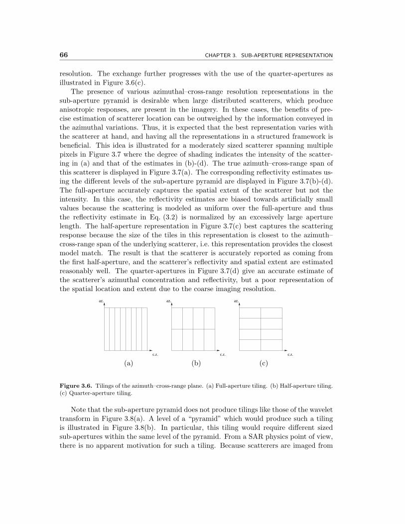
66 CHAPTER 3. SUB-APERTURE REPRESENTATION
resolution. The exchange further progresses with the use of the quarter-apertures asillustrated in Figure 3.6(c).
The presence of various azimuthal–cross-range resolution representations in thesub-aperture pyramid is desirable when large distributed scatterers, which produceanisotropic responses, are present in the imagery. In these cases, the benefits of pre-cise estimation of scatterer location can be outweighed by the information conveyed inthe azimuthal variations. Thus, it is expected that the best representation varies withthe scatterer at hand, and having all the representations in a structured framework isbeneficial. This idea is illustrated for a moderately sized scatterer spanning multiplepixels in Figure 3.7 where the degree of shading indicates the intensity of the scatter-ing in (a) and that of the estimates in (b)-(d). The true azimuth–cross-range span ofthis scatterer is displayed in Figure 3.7(a). The corresponding reflectivity estimates us-ing the different levels of the sub-aperture pyramid are displayed in Figure 3.7(b)-(d).The full-aperture accurately captures the spatial extent of the scatterer but not theintensity. In this case, the reflectivity estimates are biased towards artificially smallvalues because the scattering is modeled as uniform over the full-aperture and thusthe reflectivity estimate in Eq. (3.2) is normalized by an excessively large aperturelength. The half-aperture representation in Figure 3.7(c) best captures the scatteringresponse because the size of the tiles in this representation is closest to the azimuth–cross-range span of the underlying scatterer, i.e. this representation provides the closestmodel match. The result is that the scatterer is accurately reported as coming fromthe first half-aperture, and the scatterer’s reflectivity and spatial extent are estimatedreasonably well. The quarter-apertures in Figure 3.7(d) give an accurate estimate ofthe scatterer’s azimuthal concentration and reflectivity, but a poor representation ofthe spatial location and extent due to the coarse imaging resolution.
c.r.
az.
c.r.
az.
c.r.
az.
(a) (b) (c)
Figure 3.6. Tilings of the azimuth–cross-range plane. (a) Full-aperture tiling. (b) Half-aperture tiling.(c) Quarter-aperture tiling.
Note that the sub-aperture pyramid does not produce tilings like those of the wavelettransform in Figure 3.8(a). A level of a “pyramid” which would produce such a tilingis illustrated in Figure 3.8(b). In particular, this tiling would require different sizedsub-apertures within the same level of the pyramid. From a SAR physics point of view,there is no apparent motivation for such a tiling. Because scatterers are imaged from
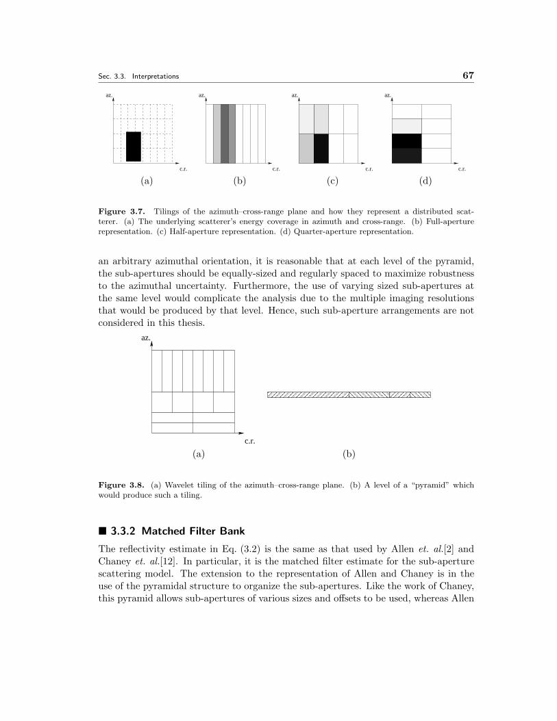
Sec. 3.3. Interpretations 67
c.r.
az.
c.r.
az.
c.r.
az.
c.r.
az.
(a) (b) (c) (d)
Figure 3.7. Tilings of the azimuth–cross-range plane and how they represent a distributed scat-terer. (a) The underlying scatterer’s energy coverage in azimuth and cross-range. (b) Full-aperturerepresentation. (c) Half-aperture representation. (d) Quarter-aperture representation.
an arbitrary azimuthal orientation, it is reasonable that at each level of the pyramid,the sub-apertures should be equally-sized and regularly spaced to maximize robustnessto the azimuthal uncertainty. Furthermore, the use of varying sized sub-apertures atthe same level would complicate the analysis due to the multiple imaging resolutionsthat would be produced by that level. Hence, such sub-aperture arrangements are notconsidered in this thesis.
c.r.
az.
������������������������������������������������������������������������
������������������������������������
��������������������
��������������������
(a) (b)
Figure 3.8. (a) Wavelet tiling of the azimuth–cross-range plane. (b) A level of a “pyramid” whichwould produce such a tiling.
� 3.3.2 Matched Filter Bank
The reflectivity estimate in Eq. (3.2) is the same as that used by Allen et. al.[2] andChaney et. al.[12]. In particular, it is the matched filter estimate for the sub-aperturescattering model. The extension to the representation of Allen and Chaney is in theuse of the pyramidal structure to organize the sub-apertures. Like the work of Chaney,this pyramid allows sub-apertures of various sizes and offsets to be used, whereas Allen
68 CHAPTER 3. SUB-APERTURE REPRESENTATION
uses a fixed sub-aperture size. Thus, Allen’s representation corresponds to a particularlevel of a sub-aperture pyramid.
The sub-aperture pyramid is also similar in spirit to Benitz’s high definition vec-tor imaging (HDVI)[5, 6]. For both the sub-aperture pyramid and HDVI, reflectivitiesare estimated based on various scattering hypotheses and are used to form a vectorof reflectivity images. A notable difference between the two approaches is that HDVIuses super-resolution techniques to achieve a resolution that exceeds the Fourier limitin Eqs. (2.3) and (2.6), whereas the sub-aperture pyramid is based on the conventionalbeamformer and thus does not exceed the Fourier limit. Super-resolution techniquesare not used in the pyramid representation because they are not consistent in theirhandling of anisotropic scatterers. In particular, as discussed in Section 2.3, super-resolution techniques are designed to suppress the interference from neighboring pointscatterers even when the steering vector is adapted to anisotropic, and hence spatiallyextended, scatterers. The suppression of interference is specifically tuned to that frompoint scatterers because of the manner in which the data correlation matrix is esti-mated. The method assumes stationarity in frequency and azimuth which is equivalentto frequency independent, isotropic scattering. As a result, these methods tend toartificially break up spatially distributed scatterers in the imagery. Because it is theaim of this thesis to develop robust methods to exploit anisotropy, the more consistentconventional beamformer is used to estimate reflectivity.
Chapter 4
Nonparametric Estimation ofAnisotropy
This chapter presents a SAR classifier adapted to exploit scatterer anisotropy from thedensity-based classification idea discussed in Section 2.4.3. The feature vector used inthis classifier is obtained from a sub-aperture pyramid of Section 3.1 in order to exploitanisotropic phenomena. In particular, sub-aperture reflectivities are estimated overthe entire image to reveal the azimuthal variations produced by the scatterers on atarget. The Parzen density estimator is then used to learn the distribution of the sub-aperture reflectivities. The resulting density estimate implicitly describes the anisotropyexhibited by the target in the image. Thus, by comparing the density estimate from anunlabeled target image to density estimates from labeled target images, a classificationbased upon anisotropy behavior is obtained.
The classification approach presented in this chapter is a modification of the ap-proach proposed by DeBonet et. al.[20] which is summarized in Appendix A. The mostsignificant difference between the two approaches is in the choice of the feature vector.DeBonet uses a multiresolution wavelet-based feature set obtained through the applica-tion of oriented edge-filters to the log-magnitude image data at multiple resolutions. Inparticular, the feature vector for a given location is taken as the set of edge-filter outputscorresponding to the specified location. Use of such a feature set reveals the orientedvisual texture of images as discussed by DeBonet et. al. in [19]. Like the wavelet-basedfeature vector used by DeBonet, the sub-aperture feature vector used in this chapter isalso multiresolution in nature due to the use of apertures of varying lengths. However,the use of the sub-aperture feature vector is motivated by radar scattering physics incontrast to image texture.
The remainder of this chapter is organized as follows. Section 4.1 establishes thecontext for the classification problem considered. Section 4.2 describes the algorithmin detail including construction of the sub-aperture feature vector and implementationissues regarding the nonparametric classifier. Section 4.3 then presents results from theapplication of the proposed classifier to the MSTAR[1] data set.
69
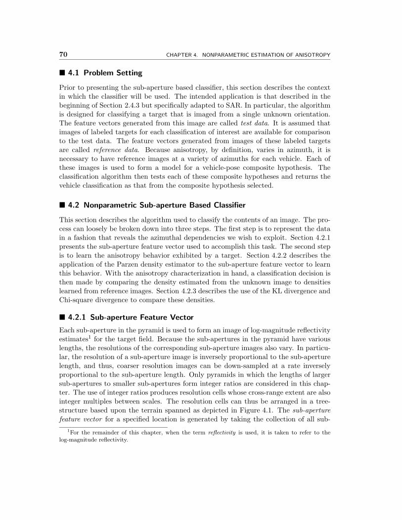
70 CHAPTER 4. NONPARAMETRIC ESTIMATION OF ANISOTROPY
� 4.1 Problem Setting
Prior to presenting the sub-aperture based classifier, this section describes the contextin which the classifier will be used. The intended application is that described in thebeginning of Section 2.4.3 but specifically adapted to SAR. In particular, the algorithmis designed for classifying a target that is imaged from a single unknown orientation.The feature vectors generated from this image are called test data. It is assumed thatimages of labeled targets for each classification of interest are available for comparisonto the test data. The feature vectors generated from images of these labeled targetsare called reference data. Because anisotropy, by definition, varies in azimuth, it isnecessary to have reference images at a variety of azimuths for each vehicle. Each ofthese images is used to form a model for a vehicle-pose composite hypothesis. Theclassification algorithm then tests each of these composite hypotheses and returns thevehicle classification as that from the composite hypothesis selected.
� 4.2 Nonparametric Sub-aperture Based Classifier
This section describes the algorithm used to classify the contents of an image. The pro-cess can loosely be broken down into three steps. The first step is to represent the datain a fashion that reveals the azimuthal dependencies we wish to exploit. Section 4.2.1presents the sub-aperture feature vector used to accomplish this task. The second stepis to learn the anisotropy behavior exhibited by a target. Section 4.2.2 describes theapplication of the Parzen density estimator to the sub-aperture feature vector to learnthis behavior. With the anisotropy characterization in hand, a classification decision isthen made by comparing the density estimated from the unknown image to densitieslearned from reference images. Section 4.2.3 describes the use of the KL divergence andChi-square divergence to compare these densities.
� 4.2.1 Sub-aperture Feature Vector
Each sub-aperture in the pyramid is used to form an image of log-magnitude reflectivityestimates1 for the target field. Because the sub-apertures in the pyramid have variouslengths, the resolutions of the corresponding sub-aperture images also vary. In particu-lar, the resolution of a sub-aperture image is inversely proportional to the sub-aperturelength, and thus, coarser resolution images can be down-sampled at a rate inverselyproportional to the sub-aperture length. Only pyramids in which the lengths of largersub-apertures to smaller sub-apertures form integer ratios are considered in this chap-ter. The use of integer ratios produces resolution cells whose cross-range extent are alsointeger multiples between scales. The resolution cells can thus be arranged in a tree-structure based upon the terrain spanned as depicted in Figure 4.1. The sub-aperturefeature vector for a specified location is generated by taking the collection of all sub-
1For the remainder of this chapter, when the term reflectivity is used, it is taken to refer to thelog-magnitude reflectivity.
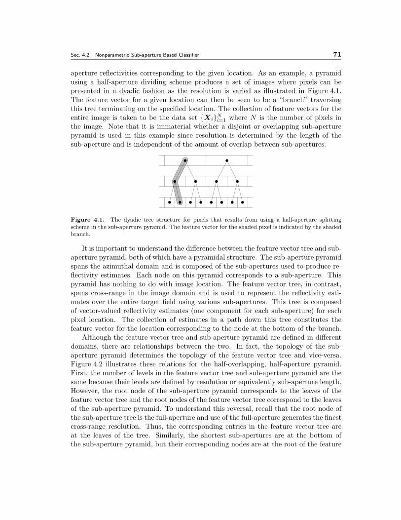
Sec. 4.2. Nonparametric Sub-aperture Based Classifier 71
aperture reflectivities corresponding to the given location. As an example, a pyramidusing a half-aperture dividing scheme produces a set of images where pixels can bepresented in a dyadic fashion as the resolution is varied as illustrated in Figure 4.1.The feature vector for a given location can then be seen to be a “branch” traversingthis tree terminating on the specified location. The collection of feature vectors for theentire image is taken to be the data set {Xi}Ni=1 where N is the number of pixels inthe image. Note that it is immaterial whether a disjoint or overlapping sub-aperturepyramid is used in this example since resolution is determined by the length of thesub-aperture and is independent of the amount of overlap between sub-apertures.
Figure 4.1. The dyadic tree structure for pixels that results from using a half-aperture splittingscheme in the sub-aperture pyramid. The feature vector for the shaded pixel is indicated by the shadedbranch.
It is important to understand the difference between the feature vector tree and sub-aperture pyramid, both of which have a pyramidal structure. The sub-aperture pyramidspans the azimuthal domain and is composed of the sub-apertures used to produce re-flectivity estimates. Each node on this pyramid corresponds to a sub-aperture. Thispyramid has nothing to do with image location. The feature vector tree, in contrast,spans cross-range in the image domain and is used to represent the reflectivity esti-mates over the entire target field using various sub-apertures. This tree is composedof vector-valued reflectivity estimates (one component for each sub-aperture) for eachpixel location. The collection of estimates in a path down this tree constitutes thefeature vector for the location corresponding to the node at the bottom of the branch.
Although the feature vector tree and sub-aperture pyramid are defined in differentdomains, there are relationships between the two. In fact, the topology of the sub-aperture pyramid determines the topology of the feature vector tree and vice-versa.Figure 4.2 illustrates these relations for the half-overlapping, half-aperture pyramid.First, the number of levels in the feature vector tree and sub-aperture pyramid are thesame because their levels are defined by resolution or equivalently sub-aperture length.However, the root node of the sub-aperture pyramid corresponds to the leaves of thefeature vector tree and the root nodes of the feature vector tree correspond to the leavesof the sub-aperture pyramid. To understand this reversal, recall that the root node ofthe sub-aperture tree is the full-aperture and use of the full-aperture generates the finestcross-range resolution. Thus, the corresponding entries in the feature vector tree areat the leaves of the tree. Similarly, the shortest sub-apertures are at the bottom ofthe sub-aperture pyramid, but their corresponding nodes are at the root of the feature
72 CHAPTER 4. NONPARAMETRIC ESTIMATION OF ANISOTROPY
vector tree since these sub-apertures give the coarsest cross-range resolution. Due tothis bijective relation for resolution, the same label m is used to denote scale in both thefeature vector tree and sub-aperture pyramid. However, to account for the difference inthe progression of resolution on the two structures, the ordering of the values of m onthe feature vector tree are reversed from that on the sub-aperture pyramid, i.e. m = Mfor the root node and m = 0 for the leaves on the feature vector tree. To prevent anyconfusion related to scale when discussing the sub-aperture pyramid and feature vectortree, the terms finer and coarser are exclusively used to refer to resolution in the imagedomain while the terms larger and smaller are used to refer to sub-aperture lengths inthe pyramid.
��������������������������������������������
��������������������������������������������������������������������������������������������������������������������������������������������������������������������
��������������������������������������������
��������������������������������������������
��������������������������������������������
������������������������������������������������������������������������������������
������������������������������������������������������������������������������������
������������������������������������������������������������������������������������
��������������������������������������������
��������������������������������������������
��������������������������������������������
m = 2
m = 1
m = 0
m = 0
m = 1
m = 2
7D vector
scalar
3D vector
of quarter-aperture estimates
of half-aperture estimates
full-aperture estimates
Figure 4.2. The relationship between (left) the half-overlapping, half-aperture sub-aperture pyramidand (right) the corresponding feature vector tree.
The number of offspring at each scale in one structure also effects the other structure.In particular, the number of children that each node on feature vector tree spawns isequal to the ratio of sub-aperture lengths between adjacent levels in the sub-aperturetree. For example, any covering with half-aperture splitting produces a binary treeof feature vectors. Furthermore, the number of sub-apertures for a given level in thesub-aperture pyramid is equal to the dimensionality of the nodes at the associated scalein the feature vector tree since each sub-aperture produces a reflectivity estimate.
� 4.2.2 Density Estimation
From a collection of sub-aperture feature vectors, the generating density is estimatedusing the Parzen density estimator described in Section 2.4.1. In particular, the densityestimate at a point X is given by,
f(X) =1
NV
N∑i=1
K(X −Xi;h) (4.1)
where V is a normalizing volume factor, h = [h(0), . . . , h(M)] is the kernel width param-eter, and K is the hyper-rectangle kernel given by
K(y;h) =
{1 : if ∀m, ‖y(m)‖∞ < h(m),
0 : otherwise(4.2)
where y(m) represents the sub-vector of y whose components correspond to scale m,and h(m) represents the kernel width used for all feature vector components at scale m.
Sec. 4.2. Nonparametric Sub-aperture Based Classifier 73
Thus, the kernel corresponds to an indicator function conveying whether or not the datapoint y is in the hyper-rectangle whose side-length is 2h(m) for components at scale m.In order for the density estimator in Eq. (4.1) to integrate to one, the normalizationfactor V must correspond to the volume of the hyper-rectangle. Thus, V is simply
V =∏
Sm,i∈S2h(m).
In the approach presented in this chapter, h is a constant parameter. The procedurefor determining h is discussed later in Section 4.2.5
The combination of the use of the hyper-rectangle kernel and the tree structureon the feature vectors affords a computationally efficient method for estimating thedensity. In particular, computing the distances used in the Parzen kernel in a top-downmanner on the feature vector tree allows for the density estimation for each X to bedone in O(N1 log(N2)) instead of O(N1N2) where N1 and N2 are the number of pixelsin down-range and cross-range respectively.
� 4.2.3 Density Comparison
Two divergence measures are used in this chapter to compare estimated test and ref-erence densities to make a classification decision. A natural method is to use the KLdivergence discussed in Section 2.4 via the decision rule in Eq. (2.26), i.e.
l =
{l∗ � argminl
{D(f0‖fl)
}: if D(f0‖fl∗) ≤ T
none of the available hypotheses are true : otherwise(4.3)
which we will call the KLD rule. This rule approximates the ML hypothesis test witha “none of the above” decision if no hypothesis is likely enough. Although well moti-vated, recall that approximating the ML decision rule as selecting the hypothesis withminimum KL divergence in Eq. (4.3) requires the assumption of independent featurevectors. This assumption, however, does not hold due to the multiresolution nature ofthe feature vector. The violation of this assumption is especially clear in the case oftree-structured features where neighboring feature vectors share coarser scale compo-nents as illustrated in Figure 4.1. Thus, motivated by the work of DeBonet et. al.[20],this chapter also investigates the use of the Chi-square divergence as a replacement forthe KL divergence. In particular, the KLD rule in Eq. (4.3) is replaced by
l =
{l∗ � argminl
{χ2(fl, f0)
}: if χ2(fl∗ , f0) ≤ T
none of the available hypotheses are true : otherwise,(4.4)
where χ2 is the Chi-square divergence given by
χ2(fl, f0) =∫ (
fl(X)− f0(X))2
fl(X)dX (4.5)
74 CHAPTER 4. NONPARAMETRIC ESTIMATION OF ANISOTROPY
which is a second-order approximation of two times the KL divergence[15] 2D(f0‖fl∗).The rule in Eq. (4.4) will be called the χ2 rule. The performance of both the KLD andχ2 rules are examined in Section 4.3.
� 4.2.4 Feature Space Discretization
Calculation of both the KL and χ2 divergences involve an integration over the entiresample space which is computationally intensive due to the nonparametric nature ofthe density estimates. Thus, an approximation to the integral is taken. As described inAppendix A, DeBonet approximates the χ2 divergence2 by replacing the integral witha weighted summation evaluated at the reference data samples. By the law of largenumbers (LLN), this estimate of χ2 divergence converges to the true value. Althoughthis approximation is well motivated, there is a subtle, but significant, drawback tothis approach. The problem lies in the fact that the observed data samples arise froma mixture density. In particular, only a fraction of the pixels in the image cover thevehicle to be classified. The rest of the pixels cover some form of clutter such as theterrain, trees, or other nuisance scatterers. Thus, the density generating the observeddata samples can be written as the mixture
fl = agc + (1− a)gl
where gl represents the density solely for the target l, gc represents the density forclutter, and a represents the amount of clutter contamination in the observed data. Inmany instances, clutter constitutes a significant fraction of the mixture density. Forexample, the MSTAR data used at the end of this chapter has a contamination factoron the order of 90%. Thus, most of the sample points that DeBonet uses to estimatethe χ2 divergence correspond to clutter.
This misallocation of resources in the approximation motivates this thesis to takean alternative approach to estimating the KL and χ2 divergences. The approach usedhere is a Riemannian approximation to the integral instead of a LLN-motivated approx-imation. In particular, instead of evaluating the summation at reference data samplepoints, a pre-determined set of points called evaluation points are used. The evaluationpoints are generated using a modification of the k-means algorithm3[27] to producea collection of points that are approximately uniformly spaced. Letting k denote thenumber of evaluation points to choose, the steps in the procedure are illustrated inthe flow diagram in Figure 4.3. First, k evaluation points are initialized in Step 1 bysetting them to randomly chosen training vectors. Regions are then defined in Step 2by assigning each training vector to the closest evaluation point where “closeness” ismeasured in terms of the supremum norm since a hyper-rectangle is used for the densityestimation. Each of the evaluation points is then redefined in Step 3 to be the centerof its corresponding region, i.e. the center of the smallest bounding box containing all
2DeBonet uses the χ2 divergence instead of the KL divergence as his score function, but his approx-imation method is easily adapted to approximating KL divergence.
3The k-means algorithm is also known as the Generalized Lloyd Algorithm.
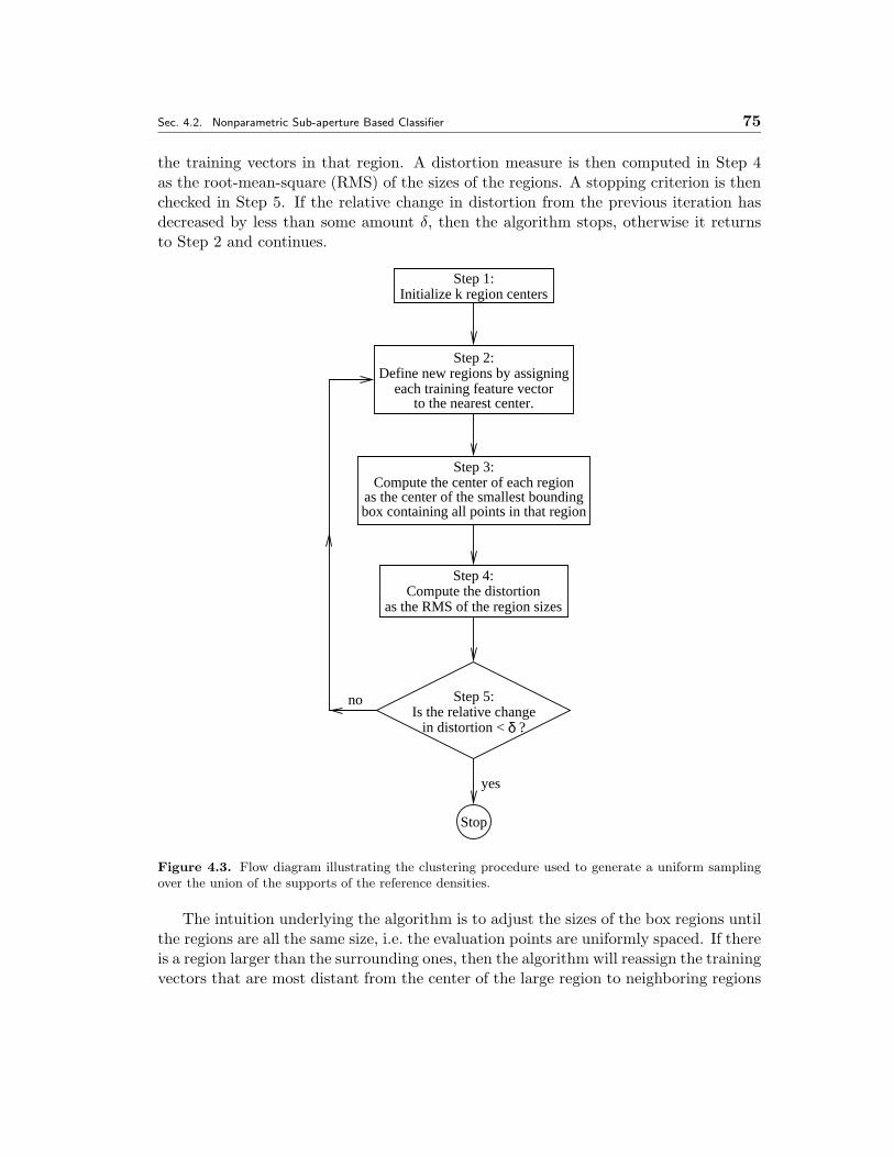
Sec. 4.2. Nonparametric Sub-aperture Based Classifier 75
the training vectors in that region. A distortion measure is then computed in Step 4as the root-mean-square (RMS) of the sizes of the regions. A stopping criterion is thenchecked in Step 5. If the relative change in distortion from the previous iteration hasdecreased by less than some amount δ, then the algorithm stops, otherwise it returnsto Step 2 and continues.
Step 2:Define new regions by assigning
each training feature vectorto the nearest center.
Step 3:Compute the center of each region
as the center of the smallest boundingbox containing all points in that region
Step 4:Compute the distortion
as the RMS of the region sizes
Stop
yes
Step 5:Is the relative change
δin distortion < ?
no
Step 1:Initialize k region centers
Figure 4.3. Flow diagram illustrating the clustering procedure used to generate a uniform samplingover the union of the supports of the reference densities.
The intuition underlying the algorithm is to adjust the sizes of the box regions untilthe regions are all the same size, i.e. the evaluation points are uniformly spaced. If thereis a region larger than the surrounding ones, then the algorithm will reassign the trainingvectors that are most distant from the center of the large region to neighboring regions
76 CHAPTER 4. NONPARAMETRIC ESTIMATION OF ANISOTROPY
where the vectors would be closer to a region center. The effect of this reallocation isto decrease the size of the larger region at the cost of increasing the size of the smallerregion.
This procedure differs from the standard k-means algorithm in Step 3 and in thedistortion measure used. The k-means algorithm computes the centroid of each regioninstead of the center. The centroid of a region is the average of the vectors in theregion and can be thought of as the center of mass in contrast to the geometric center.The distortion measure use by the k-means algorithm is the RMS of the distancesfrom each training vector to the nearest centroid. The k-means algorithm producesa sampling that is proportional to the underlying density of the training data whichresults in many closely spaced samples where the density is large and few sparse sampleswhere the density is small. As with DeBonet’s χ2 approximation, such a proportionalallocation of evaluation points is undesirable in light of the heavy clutter contaminationin the mixture distribution producing the observed data samples.
An advantage of the proposed KL and χ2 approximation procedure over DeBonet’stechnique, is that DeBonet’s approach may tend to use an excessive number of eval-uation points. DeBonet approximates the integral with a summation evaluating thesummand at each reference data point. However, for large images, this produces anexcessively fine grid. In particular, oversampling smooth densities does not lead to sig-nificantly better approximations of the integral but does increase computational cost.However, because the approach proposed in this chapter uses a fixed number k of evo-lution points, the proposed technique does not oversample in large data sets. Furthercomputational savings over DeBonet’s approximation are achieved due to the invarianceof the set of evaluation points in the proposed approach. As described in Appendix A,DeBonet uses a set of evaluation points which varies with the hypothesis to which thetest data set is compared. Thus, the density for the test data set needs to be estimatedseveral times (once for each hypothesis) in DeBonet’s proposed classifier. To illustratethe degree of the computational savings afforded by the evaluation points, the compu-tational orders of the sub-aperture classifier and DeBonet’s classifier are compared. Forboth approaches, the computation is dominated by the density estimation of the testdata. Letting Ntest denote the number of different test data sets, i.e. the number oftimes the classifier will be run, the computational orders of the two approaches can bebroken down as follows. For the approach proposed in this chapter, density estimationfor a single point is an O(N1 log(N2)) operation due to the tree structure in cross-range.Evaluating the density at k points for each test data set leads to an
O(NtestkN1 log(N2))
algorithm to classify all the data. For DeBonet’s approach, density estimation for asingle point is in an O( log(N1N2)) operation due to the tree structure in both down-range and cross-range. The density is then estimated for the test data at N1N2 points.Furthermore, this set of N1N2 points varies with the reference data set to which the
Sec. 4.2. Nonparametric Sub-aperture Based Classifier 77
test data set is compared thus leading to an
O(NrefNtestN1N2 log(N1N2)) (4.6)
algorithm to classify all the data. Noting both the omission of the factor Nref and thereplacement of N1N2 by k (which can be much less than N1N2)4, significant compu-tational savings are achieved by using the approximation technique proposed in thissection.
� 4.2.5 Kernel Width Selection
Selection of the kernel width parameter in density estimation is a classic problem. Therehave been many approaches to address this issue which are based on cross-validationor leave-one-out techniques5 that minimize a cost criterion such as mean-integratedsquared error or entropy [50, 26, 22, 32]. The goal of such methods is to characterizeaccurately the density as a whole. There is, however, a subtle difference between densityestimation for the purpose of characterizing a source distribution and density estimationfor the purpose of discrimination. To illustrate this point, consider the two densities fand g depicted in Figure 4.4. If one is only concerned with generally characterizing eachsource distribution, then for both densities, accurately estimating the region aroundthe mode of the densities is clearly important. However, if the task is to differentiatethe behavior of these two densities, then this high probability region is not of muchimportance as the densities are quite similar in this region. The tails of the densities,in contrast, are very significant since this is where the distinguishing information lies.The importance of such low probability regions is explicit in the KL and χ2 divergenceswhere the largest contributions come when one of the densities takes on small values.This example is not academic, as constant kernel width density estimators, i.e. thosewhich do not vary the kernel width with the local sparsity of the data, must trade-offestimator variance in the tails for estimator bias in the mode as the kernel width isincreased6. Such trade-offs will effect the optimal kernel width differently dependingon how the resulting density estimates are to be used.
This thesis proposes the following discrimination-based algorithm to determine ker-nel width7. The objective of the algorithm is to find the kernel width parameter h which
4There is also a computational increase replacing log(N1N2) in DeBonet’s approach with N1 log(N2)for the algorithm proposed in this chapter, but this change is due to the feature set used and not theintegral approximation method.
5Cross-validation and leave-one-out[22, 26] are methods used to evaluate the efficacy of a learningrule. In cross-validation, one partitions the data into two sets and uses one set for the “learning”process and the other to estimate the cost of using the learned variables. In leave-one-out, one uses allbut one sample for the learning process and calculates the resulting cost for the omitted sample. Thispartitioning scheme is repeatedly performed omitting a different sample each time. The overall cost isthen estimated by averaging the costs from each iteration.
6The reader is referred to Silverman[50] for more details on the bias-variance trade-off in densityestimation.
7At the time this algorithm was developed, the author was not aware of other discrimination-motivated kernel width selection procedures for density estimation. However, since that time, it has
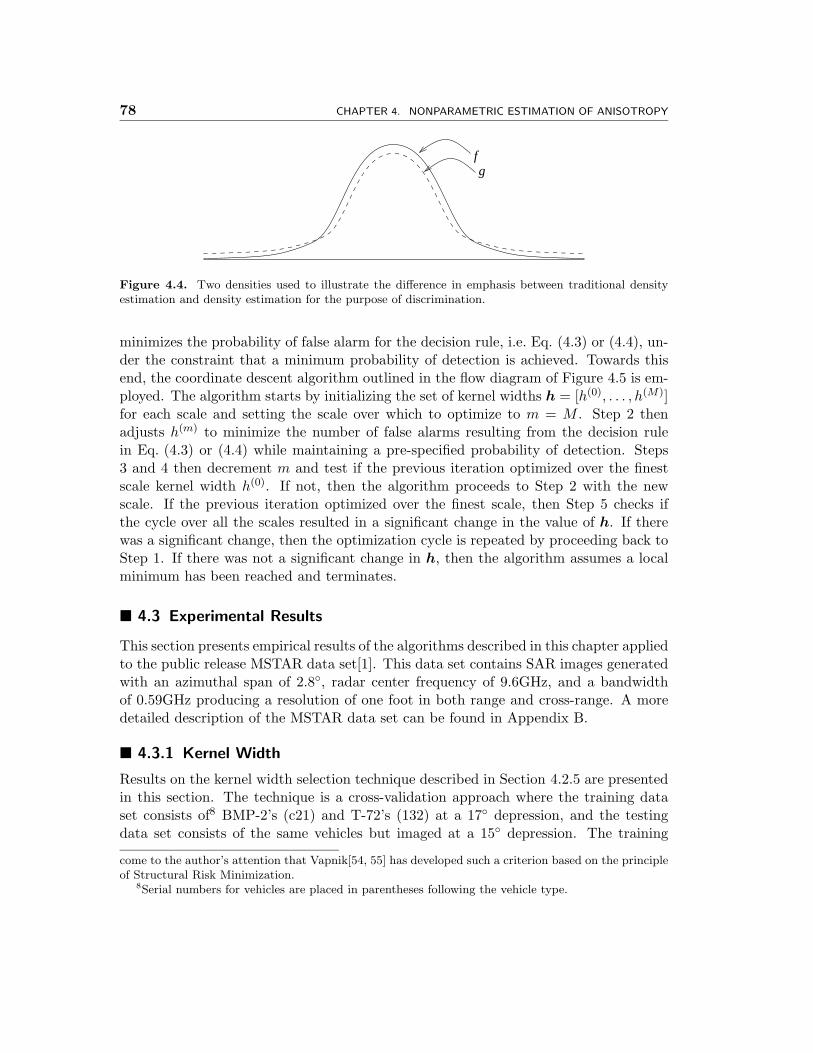
78 CHAPTER 4. NONPARAMETRIC ESTIMATION OF ANISOTROPY
fg
Figure 4.4. Two densities used to illustrate the difference in emphasis between traditional densityestimation and density estimation for the purpose of discrimination.
minimizes the probability of false alarm for the decision rule, i.e. Eq. (4.3) or (4.4), un-der the constraint that a minimum probability of detection is achieved. Towards thisend, the coordinate descent algorithm outlined in the flow diagram of Figure 4.5 is em-ployed. The algorithm starts by initializing the set of kernel widths h = [h(0), . . . , h(M)]for each scale and setting the scale over which to optimize to m = M . Step 2 thenadjusts h(m) to minimize the number of false alarms resulting from the decision rulein Eq. (4.3) or (4.4) while maintaining a pre-specified probability of detection. Steps3 and 4 then decrement m and test if the previous iteration optimized over the finestscale kernel width h(0). If not, then the algorithm proceeds to Step 2 with the newscale. If the previous iteration optimized over the finest scale, then Step 5 checks ifthe cycle over all the scales resulted in a significant change in the value of h. If therewas a significant change, then the optimization cycle is repeated by proceeding back toStep 1. If there was not a significant change in h, then the algorithm assumes a localminimum has been reached and terminates.
� 4.3 Experimental Results
This section presents empirical results of the algorithms described in this chapter appliedto the public release MSTAR data set[1]. This data set contains SAR images generatedwith an azimuthal span of 2.8◦, radar center frequency of 9.6GHz, and a bandwidthof 0.59GHz producing a resolution of one foot in both range and cross-range. A moredetailed description of the MSTAR data set can be found in Appendix B.
� 4.3.1 Kernel Width
Results on the kernel width selection technique described in Section 4.2.5 are presentedin this section. The technique is a cross-validation approach where the training dataset consists of8 BMP-2’s (c21) and T-72’s (132) at a 17◦ depression, and the testingdata set consists of the same vehicles but imaged at a 15◦ depression. The training
come to the author’s attention that Vapnik[54, 55] has developed such a criterion based on the principleof Structural Risk Minimization.
8Serial numbers for vehicles are placed in parentheses following the vehicle type.
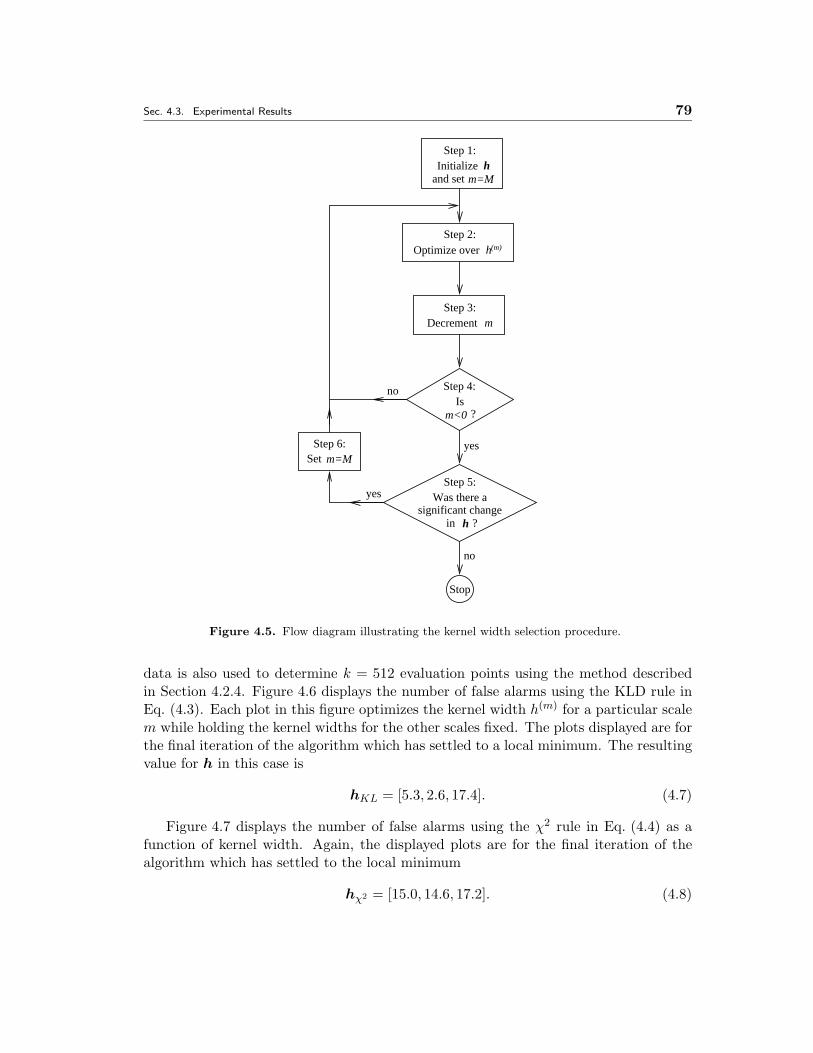
Sec. 4.3. Experimental Results 79
hm=M
Step 1:
and setInitialize
Step 3:mDecrement
Step 4:Is
m<0 ?
Step 5:Was there a
significant changein ?h
Stop
Step 6:Set m=M
no
yes
yes
no
Step 2:Optimize overh(m)
Figure 4.5. Flow diagram illustrating the kernel width selection procedure.
data is also used to determine k = 512 evaluation points using the method describedin Section 4.2.4. Figure 4.6 displays the number of false alarms using the KLD rule inEq. (4.3). Each plot in this figure optimizes the kernel width h(m) for a particular scalem while holding the kernel widths for the other scales fixed. The plots displayed are forthe final iteration of the algorithm which has settled to a local minimum. The resultingvalue for h in this case is
hKL = [5.3, 2.6, 17.4]. (4.7)
Figure 4.7 displays the number of false alarms using the χ2 rule in Eq. (4.4) as afunction of kernel width. Again, the displayed plots are for the final iteration of thealgorithm which has settled to the local minimum
hχ2 = [15.0, 14.6, 17.2]. (4.8)
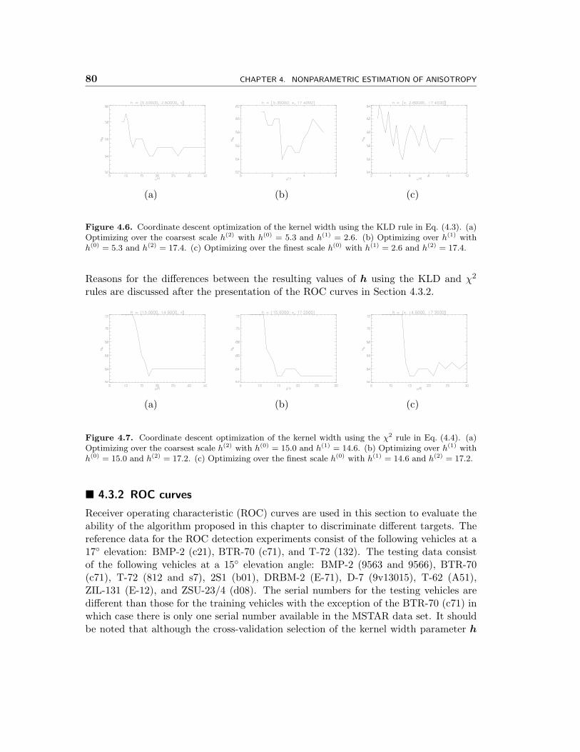
80 CHAPTER 4. NONPARAMETRIC ESTIMATION OF ANISOTROPY
(a) (b) (c)
Figure 4.6. Coordinate descent optimization of the kernel width using the KLD rule in Eq. (4.3). (a)Optimizing over the coarsest scale h(2) with h(0) = 5.3 and h(1) = 2.6. (b) Optimizing over h(1) withh(0) = 5.3 and h(2) = 17.4. (c) Optimizing over the finest scale h(0) with h(1) = 2.6 and h(2) = 17.4.
Reasons for the differences between the resulting values of h using the KLD and χ2
rules are discussed after the presentation of the ROC curves in Section 4.3.2.
(a) (b) (c)
Figure 4.7. Coordinate descent optimization of the kernel width using the χ2 rule in Eq. (4.4). (a)Optimizing over the coarsest scale h(2) with h(0) = 15.0 and h(1) = 14.6. (b) Optimizing over h(1) withh(0) = 15.0 and h(2) = 17.2. (c) Optimizing over the finest scale h(0) with h(1) = 14.6 and h(2) = 17.2.
� 4.3.2 ROC curves
Receiver operating characteristic (ROC) curves are used in this section to evaluate theability of the algorithm proposed in this chapter to discriminate different targets. Thereference data for the ROC detection experiments consist of the following vehicles at a17◦ elevation: BMP-2 (c21), BTR-70 (c71), and T-72 (132). The testing data consistof the following vehicles at a 15◦ elevation angle: BMP-2 (9563 and 9566), BTR-70(c71), T-72 (812 and s7), 2S1 (b01), DRBM-2 (E-71), D-7 (9v13015), T-62 (A51),ZIL-131 (E-12), and ZSU-23/4 (d08). The serial numbers for the testing vehicles aredifferent than those for the training vehicles with the exception of the BTR-70 (c71) inwhich case there is only one serial number available in the MSTAR data set. It shouldbe noted that although the cross-validation selection of the kernel width parameter h
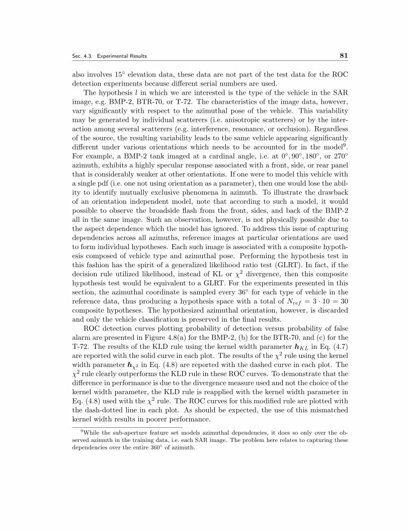
Sec. 4.3. Experimental Results 81
also involves 15◦ elevation data, these data are not part of the test data for the ROCdetection experiments because different serial numbers are used.
The hypothesis l in which we are interested is the type of the vehicle in the SARimage, e.g. BMP-2, BTR-70, or T-72. The characteristics of the image data, however,vary significantly with respect to the azimuthal pose of the vehicle. This variabilitymay be generated by individual scatterers (i.e. anisotropic scatterers) or by the inter-action among several scatterers (e.g. interference, resonance, or occlusion). Regardlessof the source, the resulting variability leads to the same vehicle appearing significantlydifferent under various orientations which needs to be accounted for in the model9.For example, a BMP-2 tank imaged at a cardinal angle, i.e. at 0◦, 90◦, 180◦, or 270◦
azimuth, exhibits a highly specular response associated with a front, side, or rear panelthat is considerably weaker at other orientations. If one were to model this vehicle witha single pdf (i.e. one not using orientation as a parameter), then one would lose the abil-ity to identify mutually exclusive phenomena in azimuth. To illustrate the drawbackof an orientation independent model, note that according to such a model, it wouldpossible to observe the broadside flash from the front, sides, and back of the BMP-2all in the same image. Such an observation, however, is not physically possible due tothe aspect dependence which the model has ignored. To address this issue of capturingdependencies across all azimuths, reference images at particular orientations are usedto form individual hypotheses. Each such image is associated with a composite hypoth-esis composed of vehicle type and azimuthal pose. Performing the hypothesis test inthis fashion has the spirit of a generalized likelihood ratio test (GLRT). In fact, if thedecision rule utilized likelihood, instead of KL or χ2 divergence, then this compositehypothesis test would be equivalent to a GLRT. For the experiments presented in thissection, the azimuthal coordinate is sampled every 36◦ for each type of vehicle in thereference data, thus producing a hypothesis space with a total of Nref = 3 · 10 = 30composite hypotheses. The hypothesized azimuthal orientation, however, is discardedand only the vehicle classification is preserved in the final results.
ROC detection curves plotting probability of detection versus probability of falsealarm are presented in Figure 4.8(a) for the BMP-2, (b) for the BTR-70, and (c) for theT-72. The results of the KLD rule using the kernel width parameter hKL in Eq. (4.7)are reported with the solid curve in each plot. The results of the χ2 rule using the kernelwidth parameter hχ2 in Eq. (4.8) are reported with the dashed curve in each plot. Theχ2 rule clearly outperforms the KLD rule in these ROC curves. To demonstrate that thedifference in performance is due to the divergence measure used and not the choice of thekernel width parameter, the KLD rule is reapplied with the kernel width parameter inEq. (4.8) used with the χ2 rule. The ROC curves for this modified rule are plotted withthe dash-dotted line in each plot. As should be expected, the use of this mismatchedkernel width results in poorer performance.
9While the sub-aperture feature set models azimuthal dependencies, it does so only over the ob-served azimuth in the training data, i.e. each SAR image. The problem here relates to capturing thesedependencies over the entire 360◦ of azimuth.
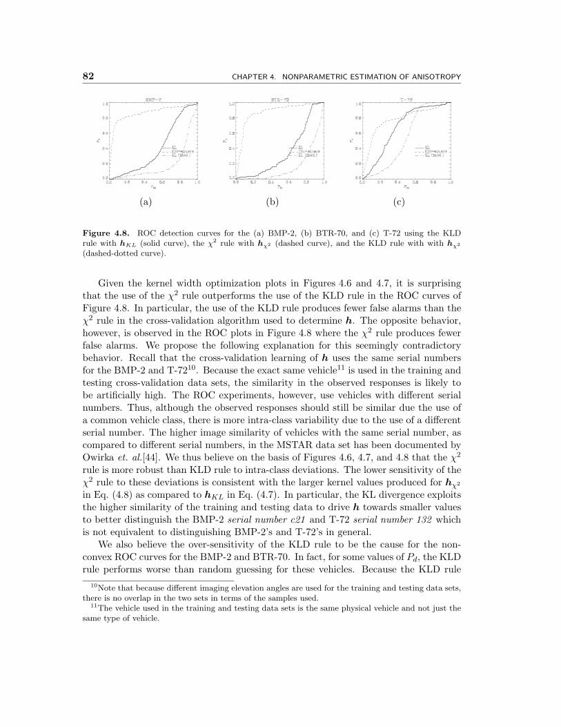
82 CHAPTER 4. NONPARAMETRIC ESTIMATION OF ANISOTROPY
(a) (b) (c)
Figure 4.8. ROC detection curves for the (a) BMP-2, (b) BTR-70, and (c) T-72 using the KLDrule with hKL (solid curve), the χ2 rule with hχ2 (dashed curve), and the KLD rule with with hχ2
(dashed-dotted curve).
Given the kernel width optimization plots in Figures 4.6 and 4.7, it is surprisingthat the use of the χ2 rule outperforms the use of the KLD rule in the ROC curves ofFigure 4.8. In particular, the use of the KLD rule produces fewer false alarms than theχ2 rule in the cross-validation algorithm used to determine h. The opposite behavior,however, is observed in the ROC plots in Figure 4.8 where the χ2 rule produces fewerfalse alarms. We propose the following explanation for this seemingly contradictorybehavior. Recall that the cross-validation learning of h uses the same serial numbersfor the BMP-2 and T-7210. Because the exact same vehicle11 is used in the training andtesting cross-validation data sets, the similarity in the observed responses is likely tobe artificially high. The ROC experiments, however, use vehicles with different serialnumbers. Thus, although the observed responses should still be similar due the use ofa common vehicle class, there is more intra-class variability due to the use of a differentserial number. The higher image similarity of vehicles with the same serial number, ascompared to different serial numbers, in the MSTAR data set has been documented byOwirka et. al.[44]. We thus believe on the basis of Figures 4.6, 4.7, and 4.8 that the χ2
rule is more robust than KLD rule to intra-class deviations. The lower sensitivity of theχ2 rule to these deviations is consistent with the larger kernel values produced for hχ2
in Eq. (4.8) as compared to hKL in Eq. (4.7). In particular, the KL divergence exploitsthe higher similarity of the training and testing data to drive h towards smaller valuesto better distinguish the BMP-2 serial number c21 and T-72 serial number 132 whichis not equivalent to distinguishing BMP-2’s and T-72’s in general.
We also believe the over-sensitivity of the KLD rule to be the cause for the non-convex ROC curves for the BMP-2 and BTR-70. In fact, for some values of Pd, the KLDrule performs worse than random guessing for these vehicles. Because the KLD rule
10Note that because different imaging elevation angles are used for the training and testing data sets,there is no overlap in the two sets in terms of the samples used.
11The vehicle used in the training and testing data sets is the same physical vehicle and not just thesame type of vehicle.
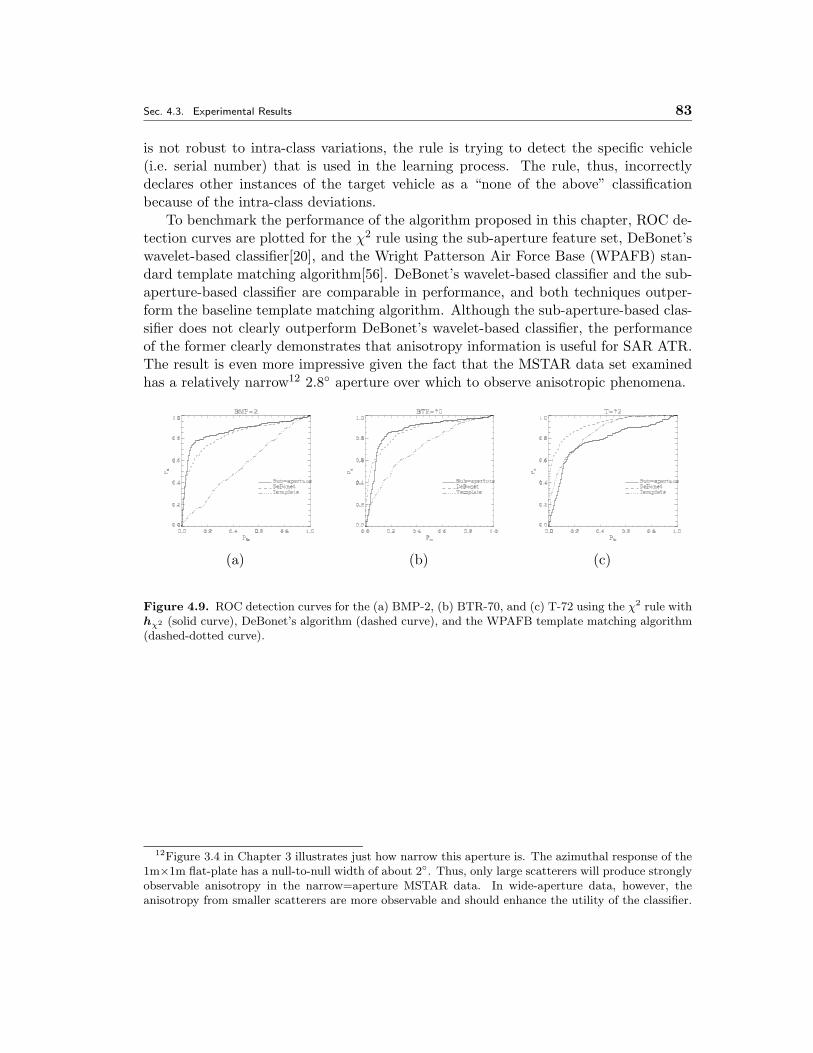
Sec. 4.3. Experimental Results 83
is not robust to intra-class variations, the rule is trying to detect the specific vehicle(i.e. serial number) that is used in the learning process. The rule, thus, incorrectlydeclares other instances of the target vehicle as a “none of the above” classificationbecause of the intra-class deviations.
To benchmark the performance of the algorithm proposed in this chapter, ROC de-tection curves are plotted for the χ2 rule using the sub-aperture feature set, DeBonet’swavelet-based classifier[20], and the Wright Patterson Air Force Base (WPAFB) stan-dard template matching algorithm[56]. DeBonet’s wavelet-based classifier and the sub-aperture-based classifier are comparable in performance, and both techniques outper-form the baseline template matching algorithm. Although the sub-aperture-based clas-sifier does not clearly outperform DeBonet’s wavelet-based classifier, the performanceof the former clearly demonstrates that anisotropy information is useful for SAR ATR.The result is even more impressive given the fact that the MSTAR data set examinedhas a relatively narrow12 2.8◦ aperture over which to observe anisotropic phenomena.
(a) (b) (c)
Figure 4.9. ROC detection curves for the (a) BMP-2, (b) BTR-70, and (c) T-72 using the χ2 rule withhχ2 (solid curve), DeBonet’s algorithm (dashed curve), and the WPAFB template matching algorithm(dashed-dotted curve).
12Figure 3.4 in Chapter 3 illustrates just how narrow this aperture is. The azimuthal response of the1m×1m flat-plate has a null-to-null width of about 2◦. Thus, only large scatterers will produce stronglyobservable anisotropy in the narrow=aperture MSTAR data. In wide-aperture data, however, theanisotropy from smaller scatterers are more observable and should enhance the utility of the classifier.

84 CHAPTER 4. NONPARAMETRIC ESTIMATION OF ANISOTROPY
Chapter 5
Sub-aperture Anisotropy Attribution
The previous chapter explored the use of the sub-aperture pyramid in a nonparametriclearning algorithm to recognize targets based upon their anisotropy behavior. However,besides the use of the sub-aperture feature set, little guidance based on intuition andunderstanding of radar scattering physics could be provided to the algorithm. Thischapter takes a different approach to exploit scatterer anisotropy for SAR ATR. Inparticular, a feature that characterizes the azimuthal location and concentration ofunimodal scattering is extracted from the data. Scattering models such as the PO modeland the GTD predict that for many scatterers, there is an inverse relationship betweenthe physical size and the azimuthal energy concentration of the scatterer[33, 48]. Theresponses for several common canonical scatterers are given in Section 2.3. Not onlyis there an inverse relation between scaling in the azimuthal and image domains, butmany canonical scatterers also produce a unimodal response along the aperture forwhich azimuthal energy concentration is a natural first-order characterization. Theproposed anisotropy feature may thus be used to provide insight about the physicalstructure of the object under investigation thereby aiding target classification.
The high level problem setting considered here is the same as that in the previ-ous chapter. In particular, we are presented with a single image of SAR data andwish to exploit the anisotropy exhibited by the target to aid the classification pro-cess. Anisotropy is exploited in this chapter by attributing the degree of anisotropy,i.e. azimuthal concentration, which conveys information about scatterer size. The basisfor this anisotropy attribution is the sub-aperture scattering model used by Chaneyet. al.[12] and Allen et. al.[2]. This model is preferred over more detailed models, suchas those based on PO and the GTD, because it provides a simple, yet intuitive, charac-terization of azimuthal scattering. Furthermore, robust estimation of the parameters inthe more complicated PO and GTD models is especially difficult in the presence of in-terfering scatterers given a limited amount of data, i.e. one image per target. Althoughbased on the sub-aperture model proposed by Chaney and Allen, the work presentedin this chapter significantly extends their efforts. These extensions include: improvingthe model for the sub-aperture measurements, accounting for the varying resolution cellsizes among the sub-apertures, modeling the interfering effects of neighboring scatter-ers, and developing a nonlinear decision-directed sub-aperture selection procedure thatpreserves high imaging resolution.
85
86 CHAPTER 5. SUB-APERTURE ANISOTROPY ATTRIBUTION
The remainder of this chapter is organized as follows. Section 5.1 presents the mea-surement model and resulting hypothesis test for an isolated scatterer. Section 5.2extends the work to account for multiple scatterers to remove the interference fromneighboring scatterers. Section 5.3 then presents a telescopic, decision-directed mod-ification to the testing procedures presented in Sections 5.1 and 5.2 which improvesrobustness to interfering scatterers and provides simultaneous high azimuthal resolu-tion and high imaging resolution. Section 5.4 concludes the chapter by applying thenew anisotropy attribution to MSTAR data.
� 5.1 Anisotropy Attribution – Isolated Scatterer Model
The sub-aperture pyramid is introduced in Chapter 3 which emphasizes the structureof the pyramid and how anisotropy is conveyed through the sub-aperture reflectivities.This chapter extends the use of the pyramid to also form a set of anisotropy models. Inparticular, the sub-aperture scattering models proposed by Chaney and Allen are usedto formulate a hypothesis test for anisotropy where the hypotheses are drawn directlyfrom the sub-aperture pyramid.
� 5.1.1 Observation Model
The anisotropy hypothesis tests presented in this chapter are for a pre-specified scatter-ing location. The location could come from a peak extraction process (resulting in peakscatterer anisotropy attribution) or a pre-specified grid of points (producing an imageof the exhibited anisotropy). As is the case for calculating sub-aperture reflectivity inSection 3.2, the dependence of the location parameter is removed through the use of theazimuthal response a(ω) which corresponds to a range-compressed, but not cross-rangecompressed, 1-D signal demodulated for the specified cross-range location.
As discussed in Section 2.3, the sub-aperture scattering model used by Chaneyand Allen models the azimuthal response as a constant over a sub-aperture and zeroelsewhere. The set of candidate sub-apertures in this chapter is restricted to thosecomposing the sub-aperture pyramid. In particular, each sub-aperture Sm,i in thepyramid is used to define an associated sub-aperture anisotropy hypothesis Hm,i whosemodeled response may be written as
Hm,i : a(ω) = A1Sm,i (ω) . (5.1)
where A is the complex scatterer reflectivity and 1Sm,i (ω) is the indicator function forthe sub-aperture Sm,i. This model is clearly an idealization of anisotropic scattering,but because we are only seeking a general characterization of anisotropy, this modelserves our purpose. Although these hypotheses are used to measure anisotropy, theideal isotropic scattering hypothesis is included in the hypothesis set since the full-aperture is included in the sub-aperture pyramid. The set of all possible hypothesesassociated with the sub-aperture pyramid will be denoted as H.
Sec. 5.1. Anisotropy Attribution – Isolated Scatterer Model 87
A reasonable choice of observations to test these hypotheses would be the set of allthe measured sub-aperture reflectivities {qm,i} where qm,i is given in Eq. (3.1) as
qm,i =∫Sm,i
a(ω) dω . (5.2)
From this definition of the qm,i and the partition property on the pyramid in Section 3.1,it is sufficient to consider the vector qM � {qm,i}m=M of measurements from the small-est sub-apertures. This vector is sufficient because any sub-aperture reflectivity qm,i
can be computed from qM by summing all the qM,j for which the associated SM,j forma partition of Sm,i, i.e.
qm,i =∑
j∣∣SM,j∈P(m,i)
qM,j . (5.3)
For example, in the three-level, half-overlapping, half-aperture pyramid in Figure 3.3(b),q1,1 = q2,2+ q2,4 since S2,2 and S2,4 form a disjoint union of S1,1. Because qM is a suffi-cient statistic, this vector is taken as the observation on which the anisotropy hypothesistest is based.
The value of the observation vector qM under hypothesis Hm,i with a normalizedreflectivity of A = 1 is denoted as b(m, i), and the jth element of b(m, i) is given by
b(m, i)j =∫SM,j
1Sm,i (ω) dω
= λ(SM,j ∩ Sm,i), (5.4)
where λ denotes Lebesgue measure. Thus, the observed response is proportional to theamount of overlap between the sub-aperture SM,j used to measure the reflectivity andthe sub-aperture Sm,i used to model the azimuthal response.
Up to this point, noise in the measurements has been omitted. The noise is nowmodeled as an additive white process along the aperture. In particular, the scatteringmodel conditioned on anisotropy hypothesis Hm,i is
qM,j =∫SM,j
[A1Sm,i (ω) + η(ω)
]dω , (5.5)
where η(ω) is circularly complex white Gaussian noise with spectral density 2σ2. Eq. (5.5)leads to the model
qM = Ab(m, i) + εεε, with εεε ∼ N (0, 2σ2Λ), (5.6)
where εεε is the measurement noise in the smallest sub-apertures and Λ is the normalizednoise covariance matrix inherited from the sub-aperture pyramid. From Eq. (5.5), itfollows that the noise εεε in Eq. (5.6) is characterized as a zero-mean circularly complex
88 CHAPTER 5. SUB-APERTURE ANISOTROPY ATTRIBUTION
Gaussian. The covariance between elements of εεε are dictated by the amount of sub-aperture overlap. In particular, the elements of the normalized matrix Λ are given bythe amount of overlap between the sub-apertures used to generate the measurements,i.e.
[Λ]i,j = λ(SM,i ∩ SM,j). (5.7)
For the case of the disjoint pyramid, Λ is the a scalar multiple of the identity matrix,i.e. Λ = 2−MI. For the case of the half-overlapping half-aperture pyramid, Λ is theToeplitz matrix
Λ =12M
1 .5
.5. . . . . .. . . . . . .5
.5 1
. (5.8)
� 5.1.2 Hypothesis Test Example
Prior to developing the anisotropy hypothesis test in its general form, the generalizedlog-likelihood ratio (GLLR) is determined for the special case of a three-level, disjoint,half-aperture pyramid as an example. For simplicity, only three of the sub-aperturehypotheses are examined. These hypotheses are the full-aperture hypothesis H0,0, theleft-most half-aperture hypothesis H1,0, and the left-most quarter-aperture hypothesisH2,0. The model for the observation vector q2 for each of these hypotheses is the Gaus-sian random vector described in Eq. (5.6). Note that there is the unknown reflectivityparameter A in the observation model. To address this unknown parameter, a GLLR isused which replaces A with its maximum likelihood (ML) estimate under each hypoth-esis, i.e. for hypothesis Hm,i, A is taken as the matched-filter estimate A = qm,i/Lm,i.The generalized likelihood ;m,i for each of the three hypothesis can then be specified asfollows
;0,0 = p (q2|H0,0, A = q0,0)
=1
|2πσ2|D/2exp
[ −14σ2
(q2 −
q0,04
[1, 1, 1, 1]T)H
Λ−1(q2 −
q0,04
[1, 1, 1, 1]T)]
=1
|2πσ2|D/2exp
[ −116σ2
(∣∣∣q2,0 − q0,04
∣∣∣2 + ∣∣∣q2,1 − q0,04
∣∣∣2 + ∣∣∣q2,2 − q0,04
∣∣∣2+∣∣∣q2,3 − q0,0
4
∣∣∣2)]
Sec. 5.1. Anisotropy Attribution – Isolated Scatterer Model 89
;1,0 = p(q2
∣∣∣H1,0, A = 2q1,0)
=1
|2πσ2|D/2exp
[ −14σ2
(q2 −
q1,02
[1, 1, 0, 0]T)H
Λ−1(q2 −
q1,02
[1, 1, 0, 0]T)]
=1
|2πσ2|D/2exp
[ −116σ2
(∣∣∣q2,0 − q1,02
∣∣∣2 + ∣∣∣q2,1 − q1,02
∣∣∣2 + |q2,2|2 + |q2,3|2)]
;2,0 = p(q2
∣∣∣H2,0, A = 4q2,0)
=1
|2πσ2|D/2exp
[ −14σ2
(q2 − q2,0[1, 0, 0, 0]T
)HΛ−1
(q2 − q2,0[1, 0, 0, 0]T
)]=
1|2πσ2|D/2
exp[ −116σ2
(|q2,1|2 + |q2,2|2 + |q2,3|2)]
where D is the dimensionality of q2, (·)T denotes transposition, (·)H denotes Hermitiantransposition, and p(·) is the Gaussian density for the observation vector conditionedon the underlying reflectivity A and anisotropy hypothesis. In each case, the likeli-hood simply measures the norm of the deviation in the smallest sub-apertures fromthe expected value under the given hypothesis. For example, under the full-aperturehypothesis, the expected response is to observe one-quarter of the reflectivity in each ofthe quarter-apertures. Consequently, the likelihood sums the squares of the deviationsfrom this expected value since each sub-aperture measurement q2,i is formed from adisjoint sub-aperture and the measurements are thus modeled as independent.
The generalized likelihoods may be used in a GLLR test as a decision rule. Takingthe ratio with respect to the full-aperture generalized likelihood, the GLLR’s γm,i canbe written as1
γ0,0 = 0
γ1,0 = log
p(q2
∣∣∣H1,0, A = 2q1,0)
p(q2
∣∣∣H0,0, A = q0,0
)
=1
4σ2
( |q1,0|20.5
− |q0,0|2)
1The calculation involves the use of the partition property, i.e. condition (C) on the pyramid inSection 3.1.
90 CHAPTER 5. SUB-APERTURE ANISOTROPY ATTRIBUTION
γ2,0 = log
p(q2
∣∣∣H2,0, A = 4q2,0)
p(q2
∣∣∣H0,0, A = q0,0
)
=1
4σ2
( |q2,0|20.25
− |q0,0|2).
There is an interesting transition that occurs in moving from generalized likelihoodsto the GLLR’s. In particular, it should be noted that the likelihoods ;m,i involve eachof the measurements from the smallest sub-apertures. These measurements manifestthemselves in the likelihood via the incoherent sum of squared-error magnitudes, i.e. thesquared-norm of the deviation from the expected sub-aperture measurements. However,for each GLLR γm,i, all the sub-aperture measurements, except qm,i and q0,0, cancelout of the expression. In other words, the only sub-aperture measurements that remainin the GLLR are those associated with the sub-aperture hypotheses the GLLR is com-paring. In particular, the expression becomes the difference between the energy in eachsub-aperture normalized by the sub-aperture length. Thus, if the decision rule is toselect the sub-aperture with the highest GLLR, then this rule is equivalent to choosingthe sub-aperture with the largest average energy. This interpretation is quite satisfyingas it is consistent with the intuition of seeking concentrated unimodal scattering inazimuth.
� 5.1.3 GLLR
The simple form of the GLLR for the sub-aperture hypotheses in the previous sectiongeneralize in a quite straightforward manner. In particular, the GLLR is the differencebetween the average energy in sub-apertures. To show this fact, however, is quite in-volved and is the topic of this section. In particular, computation of the generalizedlikelihoods involve all of the sub-aperture measurements (not just the one sub-aperturemeasurement as the simplified GLLR may lead one to mistakenly believe). The ex-pression becomes even more complicated when an overlapping sub-aperture pyramid isused because the inverse noise covariance is no longer a scalar multiple of the identity.In fact, the inverse covariance is not even sparse in this case, and thus, each of thesummands in ;m,i involves all of the smallest sub-aperture measurements.
Although the end expressions for the GLLR’s in the previous example are intuitivelyreasonable, it is somewhat surprising that so many of the sub-aperture terms cancel,even in the more complicated case of an overlapping pyramid. As will be seen in thissection, the key to these cancelations is the use of the sub-aperture scattering modelwhich permits the normalized modeled response b(m, i) to be written as a linear functionof the noise covariance which ultimately cancels the inverse noise covariance weightingmatrix in the calculations.
In order to derive the GLLR for a general sub-aperture pyramid, some notationand simple relations must first be established. Eq. (5.3) provides a representation oflarger sub-aperture reflectivity measurements from the set of smallest sub-aperture
Sec. 5.1. Anisotropy Attribution – Isolated Scatterer Model 91
measurements due to the pyramid’s partition property. It will be more convenient torewrite Eq. (5.3) as a vector multiplication. To do this, the binary vector c(P(m, i)) isdefined. In particular, the components of c(P(m, i)) are defined as
c(P(m, i))j =
{1 : if SM,j ∈ P(m, i),0 : otherwise,
(5.9)
i.e. c(P(m, i)) indicates which components of SM constitute a partition of Sm,i. Ob-taining the sub-aperture reflectivity estimate qm,i from qM can now be done via
qm,i =∑j
c(P(m, i))jqM,j
= c(P(m, i))HqM . (5.10)
Recall from Section 5.1.1 that because of the manner in which the measured reflec-tivities qm,i are calculated, i.e. integrating over a sub-aperture, the covariance betweenthese two measurements is proportional to the amount of sub-aperture overlap. Simi-larly, because the boxcar-shaped sub-aperture scattering model is used, the componentsof the normalized model vector b(m, i)j are also given by the amount of sub-apertureoverlap between Sm,i and SM,j . Because of the consistency between the reflectivitymeasurement calculation and the sub-aperture scattering model, the noise covarianceand model basis vectors can be written in terms of each other. In particular, it followsfrom Eq. (5.4) and Eq. (5.7) that
Λ =[b(M, 0)
∣∣ b(M, 1)∣∣ . . .
∣∣ b(M,JM − 1)]
(5.11)
where JM is the number of sub-apertures at scale M . From this equation, it followsthat
b(M, i) = Λei (5.12)
where ei is the Euclidean basis vector of appropriate dimension. This relation canbe generalized to write b(m, i) for larger sub-apertures in terms of Λ using the vectorc(P(m, i)). First, note that for a particular element j of b(m, i),
b(m, i)j =∫SM,j
1Sm,i (ω) dω by definition of b(m, i)j
=∫SM,j
∑k|SM,k∈P(m,i)
1SM,k(ω) dω using Eq. (5.3)
=∑
k|SM,k∈P(m,i)
∫SM,j
1SM,k(ω) dω
=∑
k|SM,k∈P(m,i)
b(M,k)j by definition of b(m, i)j
92 CHAPTER 5. SUB-APERTURE ANISOTROPY ATTRIBUTION
i.e. the normalized model for hypothesis Hm,i can be written as a sum of models frompartitioned sub-apertures HM,k. Thus, for the entire vector
b(m, i) =∑
k|SM,k∈P(m,i)
b(M,k)
=∑
k|SM,k∈P(m,i)
Λek using Eq. (5.12)
= Λ∑
k|SM,k∈P(m,i)
ek
= Λc(P(m, i)) (5.13)
thereby obtaining the desired generalization of Eq. (5.12) to larger sub-apertures.There is one more relation that is useful in the derivation of the GLLR. In particular,
b(m, i)Hc(P(m, i)) =∑
j|SM,j∈P(m,i)
b(m, i)j
=∑
j|SM,j∈P(m,i)
∫SM,j
1m,i (ω) dω by definition of b(m, i)j
=∫Sm,i
1Sm,i (ω) dω
= Lm,i (5.14)
which says that the sum of the terms in the modeled response b(m, i) is the integral ofthe normalized sub-aperture response or equivalently the sub-aperture length.
With the necessary relations in hand, the GLLR for a sub-aperture scattering hy-pothesis is now derived. Instead of explicitly stating the assumed value of A undereach of the hypotheses, for reasons which will become apparent later, it is assumed thatthe estimated value used for A can be written as A0,0 = aH
0,0qM under H0,0 and asAm,i = aH
m,iqM under Hm,i. Included in this case are the special instances
A0,0 = q0,0 = c(P(0, 0))HqM
= the full-aperture reflectivity estimate and
Am,i = qm,i/Lm,i =1
Lm,ic(P(m, i))HqM
= the hypothesized sub-aperture reflectivity estimate
Sec. 5.1. Anisotropy Attribution – Isolated Scatterer Model 93
that are used in the example of Section 5.1.2. The GLLR can now be obtained as
γm,i = log
p(qM
∣∣∣Hm,i, A = Am,i
)p(qM
∣∣∣H0,0, A = A0,0
)
=12
[(qM − b(0, 0)A0,0)
H 12σ2
Λ−1 (qM − b(0, 0)A0,0)
− (qM − b(m, i)Am,i)H 1
2σ2Λ−1 (qM − b(m, i)Am,i)
]=
14σ2
qHM
[ (I − b(0, 0)aH
0,0
)HΛ−1
(I − b(0, 0)aH
0,0
)− (
I − b(m, i)aHm,i
)HΛ−1
(I − b(m, i)aH
m,i
) ]qM
=1
4σ2qHM
[Λ−1 − Λ−1b(0, 0)aH
0,0 − a0,0b(0, 0)HΛ−1
+ a0,0b(0, 0)HΛ−1b(0, 0)aH0,0
− Λ−1 + Λ−1b(m, i)aHm,i + am,ib(m, i)HΛ−1
− am,ib(m, i)HΛ−1b(m, i)aHm,i
]qM
=1
4σ2qHM
[− c(0, 0)aH
0,0 − a0,0c(0, 0)H + a0,0b(0, 0)Hc(0, 0)aH0,0
+ c(m, i)aHm,i + am,ic(m, i)H − am,ib(m, i)Hc(m, i)aH
m,i
]qM (5.15a)
=1
4σ2qHM
[− c(0, 0)aH
0,0 − a0,0c(0, 0)H + a0,0aH0,0
+ c(m, i)aHm,i + am,ic(m, i)H − Lm,iam,ia
Hm,i
]qM (5.15b)
=1
4σ2qHM
[[a0,0 − c(P(0, 0))][a0,0 − c(P(m0, 0))]H − c(P(0, 0))c(P(0, 0))H
−[√
Lm,iam,i − 1√Lm,i
c(P(m, i))
][√Lm,iam,i − 1√
Lm,i
c(P(m, i))
]H+
1Lm,i
c(P(m, i))c(P(m, i))H]qM . (5.15c)
where Eq. (5.15a) follows from Eq. (5.13) and L0,0 = 1, and where Eq. (5.15b) followsfrom the relation in Eq. (5.14).
As in the example in Section 5.1.2, a natural choice for A is the ML estimate underthe corresponding hypothesis, i.e. Am,i = qm,i/Lm,i = c(P(m, i))HqM/Lm,i. Using this
94 CHAPTER 5. SUB-APERTURE ANISOTROPY ATTRIBUTION
value in Eq. (5.15) leads to
γm,i =1
4σ2qHM
[1
Lm,ic(P(m, i))c(P(m, i))H
− [√
Lm,iam,i − 1√Lm,i
c(P(m, i))][√
Lm,iam,i − 1√Lm,i
c(P(m, i))]H
− c(P(0, 0))c(P(0, 0))H]qM
=1
4σ2qHM
[1
Lm,ic(P(m, i))c(P(m, i))H − c(P(0, 0))c(P(0, 0))H
]qM
=1
4σ2
[1
Lm,i|qm,i|2 − |q0,0|2
](5.16)
thus giving the previously stated result. In particular, the GLLR is proportional tothe difference between the average energy in the hypothesized sub-aperture and thefull-aperture. Furthermore, the expression for the GLLR does not make explicit use ofthe smallest sub-aperture measurements qM except to generate the reflectivity of theinvolved sub-apertures, i.e. qm,i and q0,0. Thus, increasing the number of scales or theamount of sub-aperture overlap in the pyramid does not change the statistic.
� 5.1.4 Comparison to Chaney and Allen
Using a maximum likelihood approach based on the GLLR in Eq. (5.16), the sub-aperture decision rule can now be taken as selecting the sub-aperture with the maximumaverage energy. This test is very similar to the maximum average reflectivity selectioncriterion used by Allen and Chaney but is not the same in general. In particular, Allenand Chaney maximize the normalized reflectivity, or equivalently its square
γ′2m,i = |Am,i|2 =
∣∣∣∣ qm,i
Lm,i
∣∣∣∣2=
1Lm,i
|qm,i|2Lm,i
. (5.17)
Chaney and Allen use this criterion due to its interpretation as a matched-filter and thusits maximum likelihood interpretation. However, such an interpretation requires theassumption that each sub-aperture estimate have the same variance. This assumptiondoes not hold for the model proposed in Eq. (5.5) for which the variance on a sub-aperture reflectivity estimate Am,i is inversely proportional to the sub-aperture length.Furthermore, the assumption of a variance that is constant with respect to sub-aperturelength necessarily implies an awkward correlation structure between sub-apertures (evenwhen they are disjoint). Consider, for instance, the case of the full-aperture reflectivityestimate A0,0 = q0,0 and the reflectivity estimates, A1,0 = 2q1,0 and A1,1 = 2q1,1, from
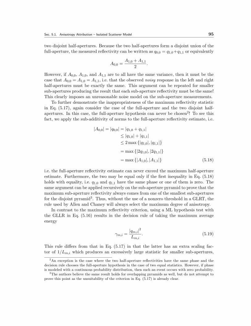
Sec. 5.1. Anisotropy Attribution – Isolated Scatterer Model 95
two disjoint half-apertures. Because the two half-apertures form a disjoint union of thefull-aperture, the measured reflectivity can be written as q0,0 = q1,0+q1,1 or equivalently
A0,0 =A1,0 +A1,1
2.
However, if A0,0, A1,0, and A1,1 are to all have the same variance, then it must be thecase that A0,0 = A1,0 = A1,1, i.e. that the observed noisy response in the left and righthalf-apertures must be exactly the same. This argument can be repeated for smallersub-apertures producing the result that each sub-aperture reflectivity must be the same!This clearly imposes an unreasonable noise model on the sub-aperture measurements.
To further demonstrate the inappropriateness of the maximum reflectivity statisticin Eq. (5.17), again consider the case of the full-aperture and the two disjoint half-apertures. In this case, the full-aperture hypothesis can never be chosen2! To see thisfact, we apply the sub-additivity of norms to the full-aperture reflectivity estimate, i.e.
|A0,0| = |q0,0| = |q1,0 + q1,1|≤ |q1,0|+ |q1,1|≤ 2max {|q1,0|, |q1,1|}= max {|2q1,0|, |2q1,1|}= max {|A1,0|, |A1,1|} (5.18)
i.e. the full-aperture reflectivity estimate can never exceed the maximum half-apertureestimate. Furthermore, the two may be equal only if the first inequality in Eq. (5.18)holds with equality, i.e. q1,0 and q1,1 have the same phase or one of them is zero. Thesame argument can be applied recursively on the sub-aperture pyramid to prove that themaximum sub-aperture reflectivity always comes from one of the smallest sub-aperturesfor the disjoint pyramid3. Thus, without the use of a nonzero threshold in a GLRT, therule used by Allen and Chaney will always select the maximum degree of anisotropy.
In contrast to the maximum reflectivity criterion, using a ML hypothesis test withthe GLLR in Eq. (5.16) results in the decision rule of taking the maximum averageenergy
γm,i =|qm,i|2Lm,i
. (5.19)
This rule differs from that in Eq. (5.17) in that the latter has an extra scaling fac-tor of 1/Lm,i which produces an excessively large statistic for smaller sub-apertures,
2An exception is the case where the two half-aperture reflectivities have the same phase and thedecision rule chooses the full-aperture hypothesis in the case of two equal statistics. However, if phaseis modeled with a continuous probability distribution, then such an event occurs with zero probability.
3The authors believe the same result holds for overlapping pyramids as well, but do not attempt toprove this point as the unsuitability of the criterion in Eq. (5.17) is already clear.
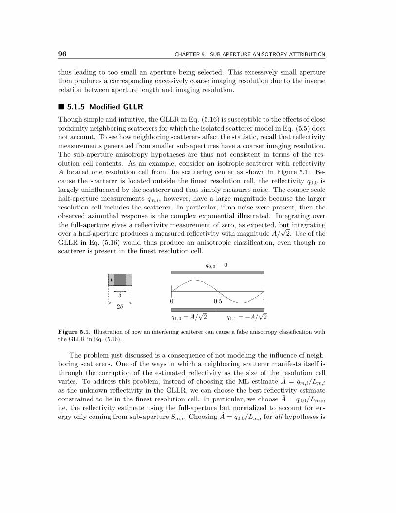
96 CHAPTER 5. SUB-APERTURE ANISOTROPY ATTRIBUTION
thus leading to too small an aperture being selected. This excessively small aperturethen produces a corresponding excessively coarse imaging resolution due to the inverserelation between aperture length and imaging resolution.
� 5.1.5 Modified GLLR
Though simple and intuitive, the GLLR in Eq. (5.16) is susceptible to the effects of closeproximity neighboring scatterers for which the isolated scatterer model in Eq. (5.5) doesnot account. To see how neighboring scatterers affect the statistic, recall that reflectivitymeasurements generated from smaller sub-apertures have a coarser imaging resolution.The sub-aperture anisotropy hypotheses are thus not consistent in terms of the res-olution cell contents. As an example, consider an isotropic scatterer with reflectivityA located one resolution cell from the scattering center as shown in Figure 5.1. Be-cause the scatterer is located outside the finest resolution cell, the reflectivity q0,0 islargely uninfluenced by the scatterer and thus simply measures noise. The coarser scalehalf-aperture measurements qm,i, however, have a large magnitude because the largerresolution cell includes the scatterer. In particular, if no noise were present, then theobserved azimuthal response is the complex exponential illustrated. Integrating overthe full-aperture gives a reflectivity measurement of zero, as expected, but integratingover a half-aperture produces a measured reflectivity with magnitude A/
√2. Use of the
GLLR in Eq. (5.16) would thus produce an anisotropic classification, even though noscatterer is present in the finest resolution cell.
δ
2δ0 0.5 1
q0,0 = 0
q1,0 = A/√2 q1,1 = −A/
√2
Figure 5.1. Illustration of how an interfering scatterer can cause a false anisotropy classification withthe GLLR in Eq. (5.16).
The problem just discussed is a consequence of not modeling the influence of neigh-boring scatterers. One of the ways in which a neighboring scatterer manifests itself isthrough the corruption of the estimated reflectivity as the size of the resolution cellvaries. To address this problem, instead of choosing the ML estimate A = qm,i/Lm,i
as the unknown reflectivity in the GLLR, we can choose the best reflectivity estimateconstrained to lie in the finest resolution cell. In particular, we choose A = q0,0/Lm,i,i.e. the reflectivity estimate using the full-aperture but normalized to account for en-ergy only coming from sub-aperture Sm,i. Choosing A = q0,0/Lm,i for all hypotheses is
Sec. 5.1. Anisotropy Attribution – Isolated Scatterer Model 97
equivalent to using Am,i = c(P(0, 0))HqM/Lm,i in Eq. (5.15) which produces
γm,i =1
4σ2qHM
{1
Lm,ic(P(m, i))c(P(m, i))H
− 1Lm,i
[c(P(0, 0))− c(P(m, i))] [c(P(0, 0))− c(P(m, i))]H
− c(P(0, 0))c(P(0, 0))H}
qM
=1
4σ2
[1
Lm,i|qm,i|2 − 1
Lm,i|q0,0 − qm,i|2 − |q0,0|2
]. (5.20)
This statistic is identical to that in Eq. (5.16) except for the extra term comparing thereflectivities q0,0 and qm,i. Recall that Eq. (5.16) compared the average energy in asub-aperture to the full-aperture. This modified GLLR accounts for the average energyoutside the hypothesized sub-aperture as well. Viewed differently, under hypothesisHm,i and the scattering model in Eqs. (5.5) and (5.6), the values of q0,0 and qm,i shouldsimply be noisy perturbations of each other. The new term in Eq. (5.20) penalizes whenthis is not the case thereby enforcing a consistency of the resolution cell contents. Forinstance, in the example in Figure 5.1, since the the contribution of each of the half-apertures would be the same, the modified GLLR is equal to zero for all hypotheses,which is reasonable since there is no underlying scattering at the focused location.
� 5.1.6 Sub-aperture Scattering Model Deviations
The sub-aperture scattering model defined in Eq. (5.1) is a simple model to which realscatterers do not exactly fit. One may question how deviations from this model affectthe resulting hypothesis tests. For example, if the scattering has a sinc(·) dependencein azimuth, then the sidelobes4 will have a large response for a strong scatterer andmay not be well modeled as the additive measurement noise εεε in Eq. (5.6). To addressthis issue, deviations from the sub-aperture scattering model are incorporated into themeasurement model. In particular, the underlying normalized scattering response isperturbed by white Gaussian noise. This perturbation changes the modeled responsein Eq. (5.4) to
b(m, i)j =∫SM,j
[1Sm,i (ω) + ν(ω)
]dω (5.21)
where ν(ω) is a white Gaussian process with spectral density 2ρ2 and is independent ofthe measurement noise η(ω). Thus, the modeled measurement vector is now a randomvector characterized as
b(m, i) ∼ N (b(m, i), 2ρ2Λ).4The term “sidelobes” here refers to those on a sinc-like function in the azimuthal domain and not
those associated with a neighboring scatterer in the image domain.
98 CHAPTER 5. SUB-APERTURE ANISOTROPY ATTRIBUTION
This modification results in the new measurement model as
Hm,i : qM = Ab(m, i) + εεε
= Ab(m, i) + w, with w ∼ N (0, 2(|A|2ρ2 + σ2)Λ). (5.22)
This is essentially the same model as in Eq. (5.6) except that the variance of the noisenow depends affinely on the square-magnitude of the underlying scatterer. Furthermore,the variance under each hypothesis scales by the same factor. Thus, the value of thenoise variance is relevant only when the GLLR is compared to a threshold other thanzero and one wishes to set the threshold based on cost (or prior probability) ratios.This modified measurement model is used throughout the remainder of the thesis.
� 5.1.7 Experimental Results
To demonstrate the behavior of the anisotropy attribution methods described in thissection, the three-level, half-overlapping, half-aperture pyramid is used to attributesynthesized SAR data. A value of ρ = 0.1 is used to account for deviations from the sub-aperture scattering model in Eq. (5.21). Anisotropy tests are applied to the synthesizeddata whose log-magnitude image (formed using the standard image formation process)is displayed in Figure 5.2(a). The position of the radar is to left of the image, andthus cross-range is the vertical dimension. The parameters for the synthesized radardata are set to nominal MSTAR parameters, i.e. an azimuthal span of 2.8◦, centerfrequency of 9.6GHz, and a bandwidth of 590MHz. The image is composed of 11scatterers, highlighted by circles in Figure 5.2(b), in circularly complex white Gaussiannoise. Each of the scatterers is generated according to the PO model for the flat platein Eq. (2.16). In particular, the following four scatterer responses are used:
• A flat plate measuring half a resolution cell in cross-range, approximately giving anisotropic response, with a signal-to-noise ratio (SNR)5 of 30dB. These scatterersare denoted by ’A’ in Figure 5.2(b).
• A flat plate measuring two resolution cells in cross-range, approximately givinga half-aperture anisotropic response, with an SNR of 30dB. These scatterers aredenoted by ’B’ in Figure 5.2(b).
• A flat plate measuring four resolution cells in cross-range, approximately givinga quarter-aperture anisotropic response, with an SNR of 30dB. These scatterersare denoted by ’C’ in Figure 5.2(b).
• A flat plate measuring two resolution cells in cross-range, approximately givinga half-aperture anisotropic response, with an SNR of 20dB. These scatterers aredenoted by ’D’ in Figure 5.2(b).
5Signal energy is taken as the square-magnitude of the full-aperture reflectivity estimate.
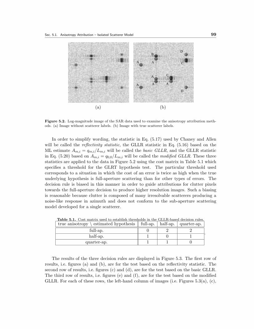
Sec. 5.1. Anisotropy Attribution – Isolated Scatterer Model 99
C
A
A
A A
A
A
BD
C
D
(a) (b)
Figure 5.2. Log-magnitude image of the SAR data used to examine the anisotropy attribution meth-ods. (a) Image without scatterer labels. (b) Image with true scatterer labels.
In order to simplify wording, the statistic in Eq. (5.17) used by Chaney and Allenwill be called the reflectivity statistic, the GLLR statistic in Eq. (5.16) based on theML estimate Am,i = qm,i/Lm,i will be called the basic GLLR, and the GLLR statisticin Eq. (5.20) based on Am,i = q0,0/Lm,i will be called the modified GLLR. These threestatistics are applied to the data in Figure 5.2 using the cost matrix in Table 5.1 whichspecifies a threshold for the GLRT hypothesis test. The particular threshold usedcorresponds to a situation in which the cost of an error is twice as high when the trueunderlying hypothesis is full-aperture scattering than for other types of errors. Thedecision rule is biased in this manner in order to guide attributions for clutter pixelstowards the full-aperture decision to produce higher resolution images. Such a biasingis reasonable because clutter is composed of many irresolvable scatterers producing anoise-like response in azimuth and does not conform to the sub-aperture scatteringmodel developed for a single scatterer.
Table 5.1. Cost matrix used to establish thresholds in the GLLR-based decision rules.true anisotropy \ estimated hypothesis full-ap. half-ap. quarter-ap.
full-ap. 0 2 2half-ap. 1 0 1
quarter-ap. 1 1 0
.
The results of the three decision rules are displayed in Figure 5.3. The first row ofresults, i.e. figures (a) and (b), are for the test based on the reflectivity statistic. Thesecond row of results, i.e. figures (c) and (d), are for the test based on the basic GLLR.The third row of results, i.e. figures (e) and (f), are for the test based on the modifiedGLLR. For each of these rows, the left-hand column of images (i.e. Figures 5.3(a), (c),
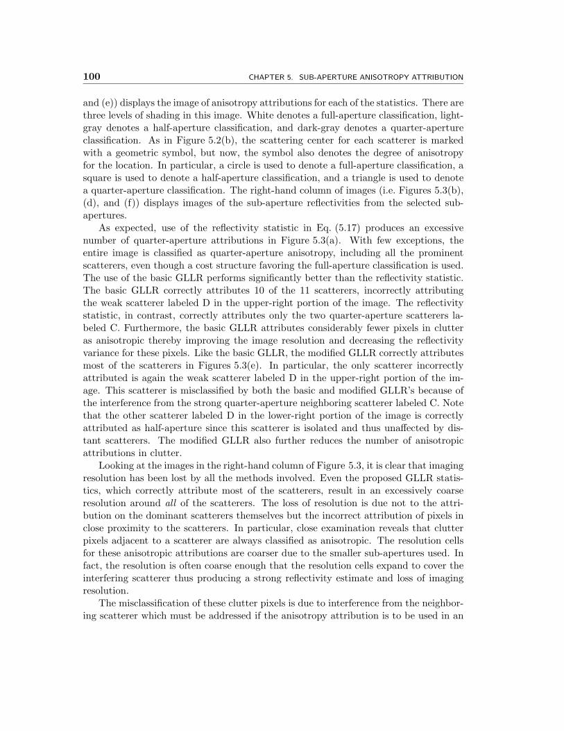
100 CHAPTER 5. SUB-APERTURE ANISOTROPY ATTRIBUTION
and (e)) displays the image of anisotropy attributions for each of the statistics. There arethree levels of shading in this image. White denotes a full-aperture classification, light-gray denotes a half-aperture classification, and dark-gray denotes a quarter-apertureclassification. As in Figure 5.2(b), the scattering center for each scatterer is markedwith a geometric symbol, but now, the symbol also denotes the degree of anisotropyfor the location. In particular, a circle is used to denote a full-aperture classification, asquare is used to denote a half-aperture classification, and a triangle is used to denotea quarter-aperture classification. The right-hand column of images (i.e. Figures 5.3(b),(d), and (f)) displays images of the sub-aperture reflectivities from the selected sub-apertures.
As expected, use of the reflectivity statistic in Eq. (5.17) produces an excessivenumber of quarter-aperture attributions in Figure 5.3(a). With few exceptions, theentire image is classified as quarter-aperture anisotropy, including all the prominentscatterers, even though a cost structure favoring the full-aperture classification is used.The use of the basic GLLR performs significantly better than the reflectivity statistic.The basic GLLR correctly attributes 10 of the 11 scatterers, incorrectly attributingthe weak scatterer labeled D in the upper-right portion of the image. The reflectivitystatistic, in contrast, correctly attributes only the two quarter-aperture scatterers la-beled C. Furthermore, the basic GLLR attributes considerably fewer pixels in clutteras anisotropic thereby improving the image resolution and decreasing the reflectivityvariance for these pixels. Like the basic GLLR, the modified GLLR correctly attributesmost of the scatterers in Figures 5.3(e). In particular, the only scatterer incorrectlyattributed is again the weak scatterer labeled D in the upper-right portion of the im-age. This scatterer is misclassified by both the basic and modified GLLR’s because ofthe interference from the strong quarter-aperture neighboring scatterer labeled C. Notethat the other scatterer labeled D in the lower-right portion of the image is correctlyattributed as half-aperture since this scatterer is isolated and thus unaffected by dis-tant scatterers. The modified GLLR also further reduces the number of anisotropicattributions in clutter.
Looking at the images in the right-hand column of Figure 5.3, it is clear that imagingresolution has been lost by all the methods involved. Even the proposed GLLR statis-tics, which correctly attribute most of the scatterers, result in an excessively coarseresolution around all of the scatterers. The loss of resolution is due not to the attri-bution on the dominant scatterers themselves but the incorrect attribution of pixels inclose proximity to the scatterers. In particular, close examination reveals that clutterpixels adjacent to a scatterer are always classified as anisotropic. The resolution cellsfor these anisotropic attributions are coarser due to the smaller sub-apertures used. Infact, the resolution is often coarse enough that the resolution cells expand to cover theinterfering scatterer thus producing a strong reflectivity estimate and loss of imagingresolution.
The misclassification of these clutter pixels is due to interference from the neighbor-ing scatterer which must be addressed if the anisotropy attribution is to be used in an
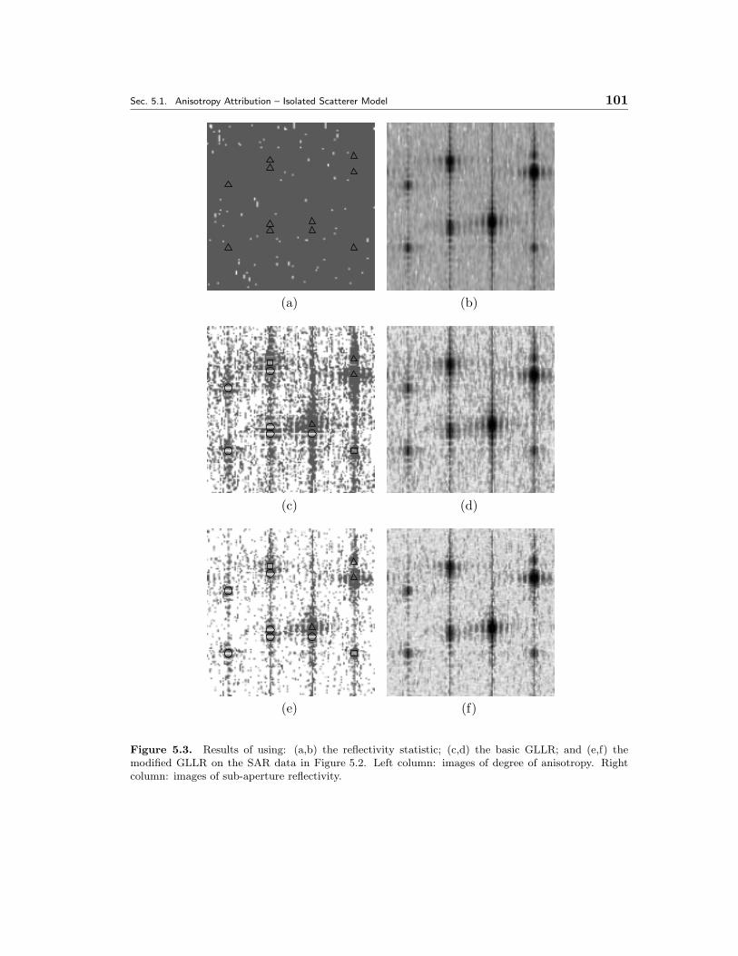
Sec. 5.1. Anisotropy Attribution – Isolated Scatterer Model 101
(a) (b)
(c) (d)
(e) (f)
Figure 5.3. Results of using: (a,b) the reflectivity statistic; (c,d) the basic GLLR; and (e,f) themodified GLLR on the SAR data in Figure 5.2. Left column: images of degree of anisotropy. Rightcolumn: images of sub-aperture reflectivity.
102 CHAPTER 5. SUB-APERTURE ANISOTROPY ATTRIBUTION
image based algorithm where resolution is important. One approach to remedy theseanisotropy misclassifications for clutter pixels is to require that a pixel’s finest resolutionreflectivity estimate exceed a particular threshold in order to be attributed. This condi-tion can be interpreted as requiring that a pre-processing step, thresholding reflectivityin this case, detect pixels that contain a scatterer and thus need to be attributed withan anisotropy label. Figure 5.4 displays the same types of images as Figure 5.3 exceptthat only pixels with a finest resolution reflectivity exceeding an SNR of 5dB are testedfor anisotropy, while all other pixels are processed with the full-aperture. The vast ma-jority of the clutter pixel misclassifications have been removed by this pre-processingstep while still allowing the prominent scatterers to be attributed. The result is animage with much higher imaging resolution that still conveys anisotropy informationfrom strong scatterers.
Unfortunately, the pre-screening step can do nothing to improved the attributionof prominent scatterers. In particular, the thresholding does nothing to correct theanisotropy attribution of the 20dB SNR scatterer labeled D in the upper-right of theimages. This scatterer is misclassified due to the interference from the stronger 30dBSNR quarter-aperture scatterer. To improve the anisotropy attribution in the presenceof neighboring scatterers, we need to explicitly account for the interference producedby the neighboring scatterers. The following sections in this chapter and Chapter 7address the handling of this interference.
� 5.2 Anisotropy Attribution – Multiple Scatterer Model
The results of the previous section demonstrate that although the use of the consis-tent (in terms of spatial coverage) reflectivity estimate Am,i = q0,0/Lm,i in place ofAm,i = qm,i/Lm,i reduces the number of false anisotropy classifications in clutter, thereare still a considerable number of misclassifications particularly surrounding a strongscatterer. These misclassifications lead to an overly coarse resolution in the imageof sub-aperture reflectivities. Because the scatterers in the image have a high SNR,the attribution of many clutter pixels can be avoided with the use of a pre-screeningthreshold on the finest resolution reflectivity. However, such a pre-processing step mightpreclude the attribution of a weak scatterer and does not improve the classification of astrong scatterer whose observed response is distorted by interference from a neighboringscatterer. To address this problem, this section focuses on improving the attributionby generalizing the anisotropy observation model and hypothesis test account for theeffects of interfering scatterers.
� 5.2.1 Model and Test
To explicitly account for interfering scatterers, the sub-aperture scattering model inEq. (5.5) must be generalized to account for the modulations produced by neighboringscatterers. To accomplish this task, we again start by assuming that the azimuthalresponse a(ω) is generated for a specified cross-range location y0. The possibility of other
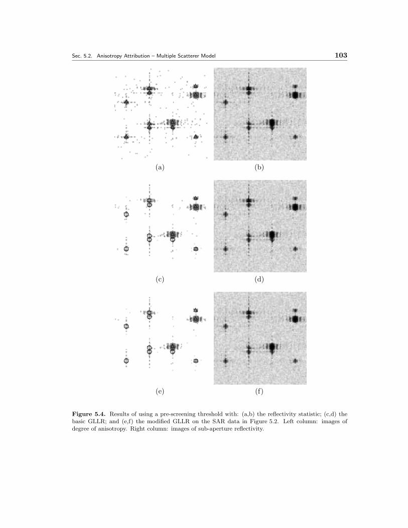
Sec. 5.2. Anisotropy Attribution – Multiple Scatterer Model 103
(a) (b)
(c) (d)
(e) (f)
Figure 5.4. Results of using a pre-screening threshold with: (a,b) the reflectivity statistic; (c,d) thebasic GLLR; and (e,f) the modified GLLR on the SAR data in Figure 5.2. Left column: images ofdegree of anisotropy. Right column: images of sub-aperture reflectivity.
104 CHAPTER 5. SUB-APERTURE ANISOTROPY ATTRIBUTION
scatterers are considered at discrete locations y0+k∆p, where ∆p specifies a cross-rangesampling resolution that is taken to be less than the full-aperture image resolution ∆r.Thus, the locations for neighboring scatterers are oversampled. Ideally, one would wantto allow the neighboring scatterers to be represented at an arbitrary location instead ofone of the pre-specified discrete locations. The former, however, significantly increasesalgorithmic complexity. The error incurred from modeling neighbors at y0 + k∆p isexpected to be small since the location error is less than one resolution cell (due to theoversampling).
To model the effect of a scatterer at location y0 + k∆p on the measurements atlocation y0, the azimuthal contribution from this neighboring scatterer is modulatedto account for the shift in the image domain. The observed effect over the smallestsub-apertures is then given by
bk(mk, ik)j =∫SM,j
ej2πk∆p∆r
ω1Hmk,ik(ω) dω (5.23)
where (mk, ik) is the sub-aperture anisotropy associated with the scatterer at y0+k∆p.Incorporation of the neighboring scatterers is now modeled via superposition, i.e.
qM =∑k
Akbk(mk, ik) + εεε (5.24)
where Ak is the reflectivity associated with the scatterer at y0 + k∆p and the noisemodel for εεε is the same as in Eq. (5.6). In order to account for all scatterers thatsignificantly affect the smallest sub-aperture measurements, the summation over k inEq. (5.24) should be over a range large enough to include all scatterers contained in thelargest resolution cell. Thus, the model should consider all k ∈ {−K, . . . ,K} where Ksatisfies
K∆p ≥ ∆r
2LM= size of coarsest resolution cell
K ≥⌈
∆r
2LM∆p
⌉(5.25)
and k = 0 corresponds to the focused resolution cell under investigation. RewritingEq. (5.24) as a matrix equation, it becomes
qM =[b−K(m−K , i−K) | · · · | bK(mK , iK)
] A−K...
AK
+ εεε
= BA + εεε (5.26)
where B and A are appropriately defined.Note that the hypotheses are now in a higher dimensional space. In particular, the
hypothesis set is now H2K+1 since each location k has an associated scatterer. For the
Sec. 5.2. Anisotropy Attribution – Multiple Scatterer Model 105
initial work presented in this chapter, the hypotheses are restricted such that only thek = 0 (the focused resolution cell) hypothesis is allowed to vary, while the hypothesesfor the other scatterers are fixed at the full-aperture hypothesis. Thus, the hypothesisspace is still H. This constraint on the anisotropy of neighbors is relaxed in Chapter 7in order to more accurately account for the contributions from neighboring scatterers.The extension, however, requires addressing several complex issues and is thus left toanother chapter.
The error εεε in Eq. (5.26) can be used to compute the likelihood of each hypothesis.The resulting set of likelihoods for all the hypotheses can then be used in a decisionrule. In particular, the error norm weighted by the inverse noise covariance, i.e. ‖εεε‖Λ−1 ,is a sufficient statistic because the noise is additive and Gaussian. The value of theerror εεε, however, is unknown and must be estimated. In the same spirit as the isolatedscattering model, εεε is estimated by first estimating A which is subsequently used tocompute εεε from Eq. (5.26), i.e.
εεε = qM −BA
where A is an estimate of A and εεε is the associated error estimate. One possibility forestimating A is ML estimation for the given hypothesis, i.e.
A = argminA
{‖εεε‖2Λ−1
}= (BHΛ−1B)−1BHΛ−1qM (5.27)
Taking A as the ML estimate, the weighted norm of the estimated error εεε becomes
‖εεε‖2Λ−1 = ‖qM −BA‖2Λ−1
=1
2σ2qHM
[Λ−1 − Λ−1B(BHΛ−1B)−1BHΛ−1
]qM (5.28)
which simplifies to the basic GLLR in Eq. (5.16) for the isolated scatterer model in thecase of limiting the model order to K = 0.
The model in Eq. (5.24) has too many parameters for the test given by the mini-mization of Eq. (5.28) to work well. In particular, if one chooses K sufficiently largeto account for all the scatterers in the coarsest resolution cell, then the model order isgreater than the number of sub-aperture measurements in qM , and thus, the estimatederror εεε can be made zero for all hypotheses. Consequently, we regularize the optimiza-tion problem. In order for the estimated error εεε to be made small under the incorrectmodel, many of the values in A generally have to be made unreasonably large whichresults in an unrealistic set of reflectivities. Thus, a 2-norm regularization penalty isused in the estimation of A. In particular, instead of minimizing the weighted squarederror to estimate A, A is estimated as
A = argminA
{‖εεε‖2Λ−1 + γAHRA}
= (BHΛ−1B + γR)−1BHΛ−1qM
= PqM (5.29)
106 CHAPTER 5. SUB-APERTURE ANISOTROPY ATTRIBUTION
where P is defined accordingly, γ is a regularization parameter, and R is the regular-ization matrix that penalizes the energy in all the Ak other than k = 0, i.e.
R = I − eKeHK = diag(1, . . . , 1, 0, 1, . . . , 1).
This regularization can be interpreted as a zero-mean Gaussian prior on the neighboringscatterer reflectivities. Use of the regularized value of A produces the following valuefor the weighted error norm
‖εεε‖2Λ−1 = ‖qM −BA‖2Λ−1
=1
2σ2qHM
[Λ−1 − 2Λ−1BP + PHBHΛ−1BP
]qM (5.30)
which can be used as the statistic in the anisotropy hypothesis test. For simplicity,the statistic in Eq. (5.30) will be called the multiple scatterer model statistic (or MSMstatistic). Note that the weighting matrix in brackets of Eq. (5.30) is data independent.Thus, the weighting matrix can be pre-computed offline for each hypothesis therebyallowing for a computationally simple likelihood that corresponds to a norm on qM .
� 5.2.2 Experimental Results
To demonstrate the performance of the anisotropy test based on the MSM statisticpresented in this section, a GLRT based on this statistic is applied to the SAR datain Figure 5.2. The number of neighboring scatterers considered is set by K = 6 andtheir spacing is set by the image oversampling rate of ∆r/∆p = 1.25. The value ofthe regularization parameter on neighboring reflectivities is set by γ = 0.5. All otherparameters are set to the same values as in Section 5.1.7.
The results of the new test are displayed in Figures 5.5 and 5.6. Figure 5.5(a) showsthe degree of anisotropy attributed, and Figure 5.5(b) shows the resulting sub-aperturereflectivity estimate. Comparing Figure 5.3 and Figure 5.5, neither of which use thepre-screening amplitude threshold, it is clear that the test using the MSM statistic bettersuppresses the number of false anisotropy classifications in clutter than the tests basedon the isolated scatterer model. Furthermore, the test using the MSM statistic stillcorrectly attributes all of the scattering centers correctly except for the weak scattererlabeled D in the upper-right portion of the image which is still attributed as quarter-aperture anisotropy. The reason this extended model does not correctly attribute thisscatterer is the neighboring scatterers are modeled as isotropic with a reflectivity thatis regularized towards zero. Consequently, the model does not fully account for theinterference from strong neighboring scatterers, and the residual interference is stillsufficient to cause a misclassification.
Results using the 5dB SNR pre-screening threshold with the new test are shownin Figure 5.6. As expected, the threshold further reduces the number of anisotropyclassifications in clutter from that in Figure 5.4 for the modified GLLR test with apre-screener and Figure 5.5 for the MSM statistic test without a pre-screener. Unfor-tunately, in all cases, there are still false anisotropy classifications for clutter pixels in
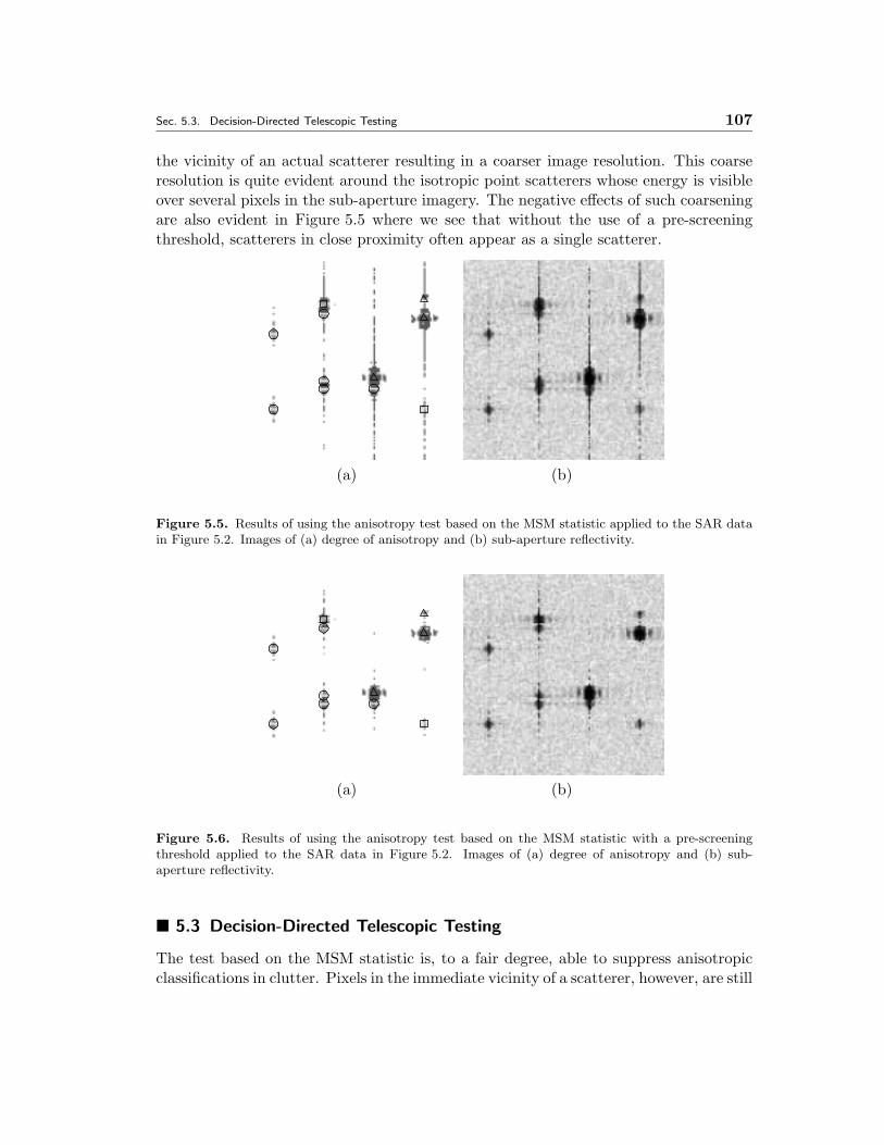
Sec. 5.3. Decision-Directed Telescopic Testing 107
the vicinity of an actual scatterer resulting in a coarser image resolution. This coarseresolution is quite evident around the isotropic point scatterers whose energy is visibleover several pixels in the sub-aperture imagery. The negative effects of such coarseningare also evident in Figure 5.5 where we see that without the use of a pre-screeningthreshold, scatterers in close proximity often appear as a single scatterer.
(a) (b)
Figure 5.5. Results of using the anisotropy test based on the MSM statistic applied to the SAR datain Figure 5.2. Images of (a) degree of anisotropy and (b) sub-aperture reflectivity.
(a) (b)
Figure 5.6. Results of using the anisotropy test based on the MSM statistic with a pre-screeningthreshold applied to the SAR data in Figure 5.2. Images of (a) degree of anisotropy and (b) sub-aperture reflectivity.
� 5.3 Decision-Directed Telescopic Testing
The test based on the MSM statistic is, to a fair degree, able to suppress anisotropicclassifications in clutter. Pixels in the immediate vicinity of a scatterer, however, are still
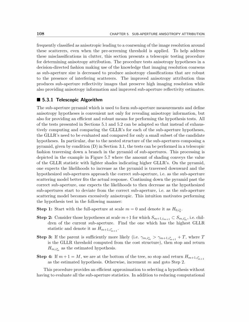
108 CHAPTER 5. SUB-APERTURE ANISOTROPY ATTRIBUTION
frequently classified as anisotropic leading to a coarsening of the image resolution aroundthese scatterers, even when the pre-screening threshold is applied. To help addressthese misclassifications in clutter, this section presents a telescopic testing procedurefor determining anisotropy attribution. The procedure tests anisotropy hypotheses in adecision-directed fashion making use of the knowledge that imaging resolution coarsensas sub-aperture size is decreased to produce anisotropy classifications that are robustto the presence of interfering scatterers. The improved anisotropy attribution thusproduces sub-aperture reflectivity images that preserve high imaging resolution whilealso providing anisotropy information and improved sub-aperture reflectivity estimates.
� 5.3.1 Telescopic Algorithm
The sub-aperture pyramid which is used to form sub-aperture measurements and defineanisotropy hypotheses is convenient not only for revealing anisotropy information, butalso for providing an efficient and robust means for performing the hypothesis tests. Allof the tests presented in Sections 5.1 and 5.2 can be adapted so that instead of exhaus-tively computing and comparing the GLLR’s for each of the sub-aperture hypotheses,the GLLR’s need to be evaluated and compared for only a small subset of the candidatehypotheses. In particular, due to the nested structure of the sub-apertures composing apyramid, given by condition (D) in Section 3.1, the tests can be performed in a telescopicfashion traversing down a branch in the pyramid of sub-apertures. This processing isdepicted in the example in Figure 5.7 where the amount of shading conveys the valueof the GLLR statistic with lighter shades indicating higher GLLR’s. On the pyramid,one expects the likelihoods to increase as the pyramid is traversed downward and thehypothesized sub-apertures approach the correct sub-aperture, i.e. as the sub-aperturescattering model better fits the actual response. Continuing down the pyramid past thecorrect sub-aperture, one expects the likelihoods to then decrease as the hypothesizedsub-apertures start to deviate from the correct sub-aperture, i.e. as the sub-aperturescattering model becomes excessively anisotropic. This intuition motivates performingthe hypothesis test in the following manner:
Step 1: Start with the full-aperture at scale m = 0 and denote it as H0,i∗0 .
Step 2: Consider those hypotheses at scalem+1 for which Sm+1,im+1 ⊂ Sm,i∗m , i.e. chil-dren of the current sub-aperture. Find the one which has the highest GLLRstatistic and denote it as Hm+1,i∗m+1
.
Step 3: If the parent is sufficiently more likely (i.e. γm,i∗m > γm+1,i∗m+1+ T , where T
is the GLLR threshold computed from the cost structure), then stop and returnHm,i∗m as the estimated hypothesis.
Step 4: If m+1 = M , we are at the bottom of the tree, so stop and return Hm+1,i∗m+1
as the estimated hypothesis. Otherwise, increment m and goto Step 2.
This procedure provides an efficient approximation to selecting a hypothesis withouthaving to evaluate all the sub-aperture statistics. In addition to reducing computational
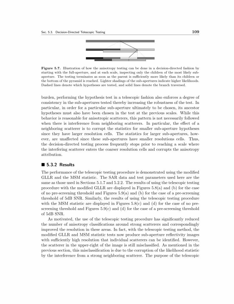
Sec. 5.3. Decision-Directed Telescopic Testing 109
Figure 5.7. Illustration of how the anisotropy testing can be done in a decision-directed fashion bystarting with the full-aperture, and at each scale, inspecting only the children of the most likely sub-aperture. The testing terminates as soon as the parent is sufficiently more likely than its children orthe bottom of the pyramid is reached. Lighter shadings of the sub-apertures indicate higher likelihoods.Dashed lines denote which hypotheses are tested, and solid lines denote the branch traversed.
burden, performing the hypothesis test in a telescopic fashion also enforces a degree ofconsistency in the sub-apertures tested thereby increasing the robustness of the test. Inparticular, in order for a particular sub-aperture ultimately to be chosen, its ancestorhypotheses must also have been chosen in the test at the previous scales. While thisbehavior is reasonable for anisotropic scatterers, this pattern is not necessarily followedwhen there is interference from neighboring scatterers. In particular, the effect of aneighboring scatterer is to corrupt the statistics for smaller sub-aperture hypothesessince they have larger resolution cells. The statistics for larger sub-apertures, how-ever, are unaffected since these sub-apertures have smaller resolutions cells. Thus,the decision-directed testing process frequently stops prior to reaching a scale wherethe interfering scatterer enters the coarser resolution cells and corrupts the anisotropyattribution.
� 5.3.2 Results
The performance of the telescopic testing procedure is demonstrated using the modifiedGLLR and the MSM statistic. The SAR data and test parameters used here are thesame as those used in Sections 5.1.7 and 5.2.2. The results of using the telescopic testingprocedure with the modified GLLR are displayed in Figures 5.8(a) and (b) for the caseof no pre-screening threshold and Figures 5.9(a) and (b) for the case of a pre-screeningthreshold of 5dB SNR. Similarly, the results of using the telescopic testing procedurewith the MSM statistic are displayed in Figures 5.8(c) and (d) for the case of no pre-screening threshold and Figures 5.9(c) and (d) for the case of a pre-screening thresholdof 5dB SNR.
As motivated, the use of the telescopic testing procedure has significantly reducedthe number of anisotropy classifications around strong scatterers and correspondinglyimproved the resolution in these areas. In fact, with the telescopic testing method, themodified GLLR and MSM statistic tests now produce sub-aperture reflectivity imageswith sufficiently high resolution that individual scatterers can be identified. However,the scatterer in the upper-right of the image is still misclassified. As mentioned in theprevious section, this misclassification is due to the corruption of the likelihood statisticby the interference from a strong neighboring scatterer. The purpose of the telescopic
110 CHAPTER 5. SUB-APERTURE ANISOTROPY ATTRIBUTION
(a) (b)
(c) (d)
Figure 5.8. Results of using the telescopic testing procedure (a-b) with the modified GLLR and (c-d)with the MSM statistic. Images of (a,c) degree of anisotropy and (b,d) sub-aperture reflectivity.
testing procedure is to reduce anisotropy classifications in clutter where interferencecauses inconsistent patterns in the likelihoods on the pyramid as the resolution cell sizevaries with scale. The processing is not specifically designed to improve the classifi-cation on strong scatterers. Consequently, it is not surprising that the attribution ofthe misclassified scatterer is not corrected by the telescopic testing procedure. The ac-counting for neighboring scatterers must be improved in order to correct this problem.This task is left to Chapter 7.
� 5.4 Results on MSTAR Data
This section presents results using the MSTAR public release data set. These imageshave a resolution of one foot in both range and cross-range that is achieved usinga transmitted signal with a 590MHz bandwidth, 9.6GHz center frequency, and 2.8◦
azimuth. This data set is described in detail in Appendix B.
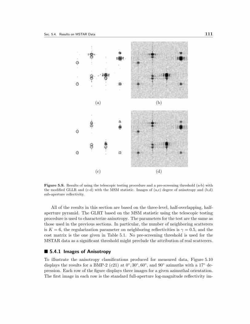
Sec. 5.4. Results on MSTAR Data 111
(a) (b)
(c) (d)
Figure 5.9. Results of using the telescopic testing procedure and a pre-screening threshold (a-b) withthe modified GLLR and (c-d) with the MSM statistic. Images of (a,c) degree of anisotropy and (b,d)sub-aperture reflectivity.
All of the results in this section are based on the three-level, half-overlapping, half-aperture pyramid. The GLRT based on the MSM statistic using the telescopic testingprocedure is used to characterize anisotropy. The parameters for the test are the same asthose used in the previous sections. In particular, the number of neighboring scatterersis K = 6, the regularization parameter on neighboring reflectivities is γ = 0.5, and thecost matrix is the one given in Table 5.1. No pre-screening threshold is used for theMSTAR data as a significant threshold might preclude the attribution of real scatterers.
� 5.4.1 Images of Anisotropy
To illustrate the anisotropy classifications produced for measured data, Figure 5.10displays the results for a BMP-2 (c21) at 0◦, 30◦, 60◦, and 90◦ azimuths with a 17◦ de-pression. Each row of the figure displays three images for a given azimuthal orientation.The first image in each row is the standard full-aperture log-magnitude reflectivity im-
112 CHAPTER 5. SUB-APERTURE ANISOTROPY ATTRIBUTION
age. The second image is a display of the anisotropy attribution at each the pixel. Thethird image is the log-magnitude of the sub-aperture reflectivity image. Even thoughthe aperture associated with this data set is relatively small at 2.8◦, anisotropy is stilldetected. In particular, it usually appears to be associated with a part of the tank. Par-ticular note is made of the exceptions at the 0◦ azimuth. Here, there are many clutterpixels classified as anisotropic. The reason that these pixels are declared as anisotropicis that the interference from neighboring large scatterer is not well modeled. Recall thatthe current formulation only considers the possibility of neighboring scatterers whichare isotropic. However, the front edge of the tank generates a very strong anisotropicresponse which is not accurately captured in our current model. Extending the modelto account for such scattering (as done in Chapter 7) should alleviate problems such asthis.
� 5.4.2 Confusion Matrices
The images in Figure 5.10 show that scatterers are being classified as anisotropic, how-ever these images do not convey how useful that information is in characterizing tar-gets. To address this issue, empirical confusion matrices for anisotropy classificationare generated using the MSTAR data set. In particular, the confusion probabilitiesare estimated from a data set composed of the following vehicles: 2S1 (b01), BMP-2 (c21), BRDM-2 (E-71), D-7 (92v13015), T-72 (132), ZIL-131 (E12), and ZSU-23/4(d08) where truth is taken as the empirical results from the 17◦ depression data andtest data is taken from the 15◦ depression data. For each pair of training and testingimages at the same azimuth, the 20 brightest peaks6 are extracted from each image anda correspondence match, based on relative location, is performed and taken as truth.The empirical confusion matrices are then computed from the anisotropy attributionsof these peaks. For the remainder of this section, the use the term “confusion matrix”refers to one computed in this fashion.
The confusion matrix for this data set is given in Table 5.2. Each row of this ma-trix represents the estimated probability distribution of the anisotropy attribution for ascatterer conditioned on the “truth” attribution of the sister vehicle. The most promi-nent aspect of this confusion matrix is the apparent independence of testing anisotropyand training anisotropy illustrated by the similarly of each row of the matrix, i.e. thenear independence on the conditioning of the training hypothesis. This result is counter-intuitive. In particular, canonical scatterer models show a strong functional dependenceof anisotropy on scatterer geometry. Consequently, we should expect the anisotropy at-tribution for these scatterers to be stable features. However, canonical scattering is notthe only source of anisotropy. Anisotropy may also arise from the interference of mul-tiple irresolvable scatterers. The conglomerate response from such a set of scatterersis a superposition of complex exponentials in azimuth. Thus, over a narrow aperture,such as the case in MSTAR data, the composite response may appear to be anisotropic.
6Peaks are taken as local maxima in the image with a minimum distance separating them.
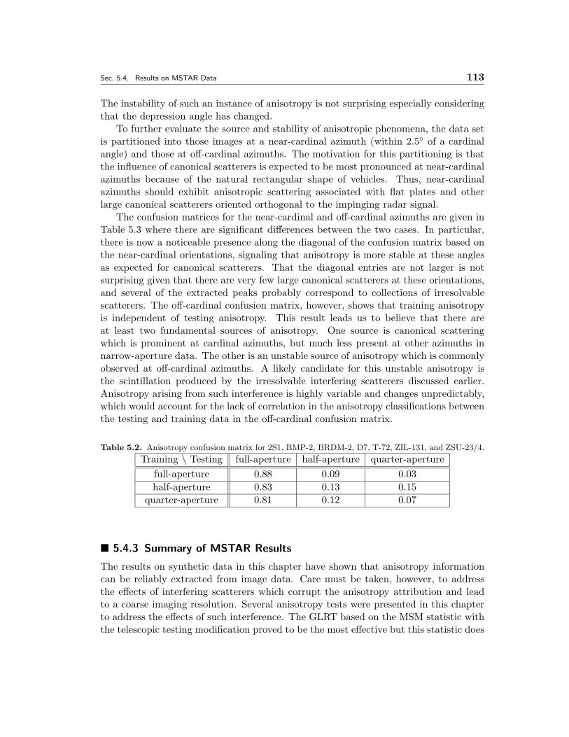
Sec. 5.4. Results on MSTAR Data 113
The instability of such an instance of anisotropy is not surprising especially consideringthat the depression angle has changed.
To further evaluate the source and stability of anisotropic phenomena, the data setis partitioned into those images at a near-cardinal azimuth (within 2.5◦ of a cardinalangle) and those at off-cardinal azimuths. The motivation for this partitioning is thatthe influence of canonical scatterers is expected to be most pronounced at near-cardinalazimuths because of the natural rectangular shape of vehicles. Thus, near-cardinalazimuths should exhibit anisotropic scattering associated with flat plates and otherlarge canonical scatterers oriented orthogonal to the impinging radar signal.
The confusion matrices for the near-cardinal and off-cardinal azimuths are given inTable 5.3 where there are significant differences between the two cases. In particular,there is now a noticeable presence along the diagonal of the confusion matrix based onthe near-cardinal orientations, signaling that anisotropy is more stable at these anglesas expected for canonical scatterers. That the diagonal entries are not larger is notsurprising given that there are very few large canonical scatterers at these orientations,and several of the extracted peaks probably correspond to collections of irresolvablescatterers. The off-cardinal confusion matrix, however, shows that training anisotropyis independent of testing anisotropy. This result leads us to believe that there areat least two fundamental sources of anisotropy. One source is canonical scatteringwhich is prominent at cardinal azimuths, but much less present at other azimuths innarrow-aperture data. The other is an unstable source of anisotropy which is commonlyobserved at off-cardinal azimuths. A likely candidate for this unstable anisotropy isthe scintillation produced by the irresolvable interfering scatterers discussed earlier.Anisotropy arising from such interference is highly variable and changes unpredictably,which would account for the lack of correlation in the anisotropy classifications betweenthe testing and training data in the off-cardinal confusion matrix.
Table 5.2. Anisotropy confusion matrix for 2S1, BMP-2, BRDM-2, D7, T-72, ZIL-131, and ZSU-23/4.
Training \ Testing full-aperture half-aperture quarter-aperturefull-aperture 0.88 0.09 0.03half-aperture 0.83 0.13 0.15
quarter-aperture 0.81 0.12 0.07
� 5.4.3 Summary of MSTAR Results
The results on synthetic data in this chapter have shown that anisotropy informationcan be reliably extracted from image data. Care must be taken, however, to addressthe effects of interfering scatterers which corrupt the anisotropy attribution and leadto a coarse imaging resolution. Several anisotropy tests were presented in this chapterto address the effects of such interference. The GLRT based on the MSM statistic withthe telescopic testing modification proved to be the most effective but this statistic does
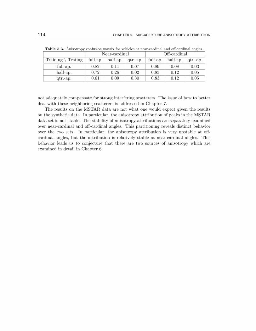
114 CHAPTER 5. SUB-APERTURE ANISOTROPY ATTRIBUTION
Table 5.3. Anisotropy confusion matrix for vehicles at near-cardinal and off-cardinal angles.
Near-cardinal Off-cardinalTraining \ Testing full-ap. half-ap. qtr.-ap. full-ap. half-ap. qtr.-ap.
full-ap. 0.82 0.11 0.07 0.89 0.08 0.03half-ap. 0.72 0.26 0.02 0.83 0.12 0.05qtr.-ap. 0.61 0.09 0.30 0.83 0.12 0.05
not adequately compensate for strong interfering scatterers. The issue of how to betterdeal with these neighboring scatterers is addressed in Chapter 7.
The results on the MSTAR data are not what one would expect given the resultson the synthetic data. In particular, the anisotropy attribution of peaks in the MSTARdata set is not stable. The stability of anisotropy attributions are separately examinedover near-cardinal and off-cardinal angles. This partitioning reveals distinct behaviorover the two sets. In particular, the anisotropy attribution is very unstable at off-cardinal angles, but the attribution is relatively stable at near-cardinal angles. Thisbehavior leads us to conjecture that there are two sources of anisotropy which areexamined in detail in Chapter 6.
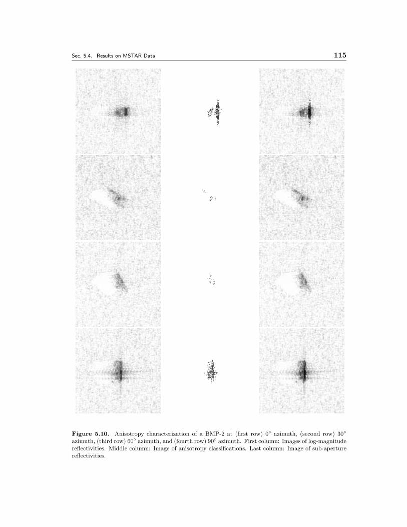
Sec. 5.4. Results on MSTAR Data 115
Figure 5.10. Anisotropy characterization of a BMP-2 at (first row) 0◦ azimuth, (second row) 30◦
azimuth, (third row) 60◦ azimuth, and (fourth row) 90◦ azimuth. First column: Images of log-magnitudereflectivities. Middle column: Image of anisotropy classifications. Last column: Image of sub-aperturereflectivities.

116 CHAPTER 5. SUB-APERTURE ANISOTROPY ATTRIBUTION
Chapter 6
Relation between Phenomenologyand Anisotropy Attribution
In the previous chapter, we observed that anisotropy attribution is considerably lessstable at off-cardinal angles than at near-cardinal angles in the MSTAR data set. Thisbehavior supports the argument for separate sources of anisotropy. This chapter ex-plores two such sources that are consistent with the observations in the MSTAR data.The two particular sources considered are geometric and volumetric scatterers. Scatter-ing models, such as the PO and GTD models, give functional forms for radar scatteringfrom canonical scatterers which clearly convey an azimuthal dependence on the shape,size, and orientation of the scatterer. These models, however, are based on very specificassumptions about the configuration of scatterer. For example, the model for a dihedralassumes two equal-sized rectangular plates conjoined to form a 90◦ angle. Our analysisof anisotropy, however, produces a more general characterization of anisotropy. Thischaracterization allows for the consideration of a broader class of scatterers that we callgeometric scatterers. This class includes not only canonical scatterers but also thosescatterers which deviate from canonicity. The other source of anisotropy considered iswhat we call volumetric scatterers. These scatterers are actually a collection of multiplescatterers which are too closely spaced to resolve as a single scatterer and thus appearas a single scatterer with an erratic azimuthal response due to the chaotic interferenceamong the constituent scatterers.
To demonstrate the scattering produced by these sources of anisotropy, Figure 6.1shows the azimuthal response from a canonical flat plate measuring 1m in cross-rangeand a volumetric scatterer composed of 10 randomly located scatterers distributedover 1m in cross-range. The flat plate response is clearly anisotropic as the azimuthalenergy is highly concentrated in the middle section of the aperture. The anisotropycharacterization of the volumetric scatterer, however, is not as clear because the az-imuthal response is less concentrated in azimuth, and the energy is erratically dis-tributed across the aperture. Figure 6.1 illustrates an important point about the “sta-bility” of anisotropy. In particular, over a relatively small aperture, such as the 2.8◦
aperture used in the MSTAR data, it is clear how the volumetric scatterer’s responsemight be classified as anisotropic as only one of the localized fluctuations is observed. If
117
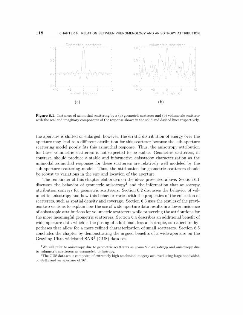
118 CHAPTER 6. RELATION BETWEEN PHENOMENOLOGY AND ANISOTROPY ATTRIBUTION
(a) (b)
Figure 6.1. Instances of azimuthal scattering by a (a) geometric scatterer and (b) volumetric scattererwith the real and imaginary components of the response shown in the solid and dashed lines respectively.
the aperture is shifted or enlarged, however, the erratic distribution of energy over theaperture may lead to a different attribution for this scatterer because the sub-aperturescattering model poorly fits this azimuthal response. Thus, the anisotropy attributionfor these volumetric scatterers is not expected to be stable. Geometric scatterers, incontrast, should produce a stable and informative anisotropy characterization as theunimodal azimuthal responses for these scatterers are relatively well modeled by thesub-aperture scattering model. Thus, the attribution for geometric scatterers shouldbe robust to variations in the size and location of the aperture.
The remainder of this chapter elaborates on the ideas presented above. Section 6.1discusses the behavior of geometric anisotropy1 and the information that anisotropyattribution conveys for geometric scatterers. Section 6.2 discusses the behavior of vol-umetric anisotropy and how this behavior varies with the properties of the collection ofscatterers, such as spatial density and coverage. Section 6.3 uses the results of the previ-ous two sections to explain how the use of wide-aperture data results in a lower incidenceof anisotropic attributions for volumetric scatterers while preserving the attributions forthe more meaningful geometric scatterers. Section 6.4 describes an additional benefit ofwide-aperture data which is the posing of additional, less anisotropic, sub-aperture hy-potheses that allow for a more refined characterization of small scatterers. Section 6.5concludes the chapter by demonstrating the argued benefits of a wide-aperture on theGrayling Ultra-wideband SAR2 (GUS) data set.
1We will refer to anisotropy due to geometric scatterers as geometric anisotropy and anisotropy dueto volumetric scatterers as volumetric anisotropy.
2The GUS data set is composed of extremely high resolution imagery achieved using large bandwidthof 4GHz and an aperture of 26◦.
Sec. 6.1. Geometric Anisotropy 119
� 6.1 Geometric Anisotropy
The behavior of geometric and volumetric anisotropy is studied in this chapter using thetelescopic anisotropy test based on the multiple scatterer model developed in Chapter 5.The analyses presented in this and the following sections are based on narrow-aperturedata because of the prevalence of such data in the SAR community. The data usedin these sections are synthesized according to MSTAR operational parameters, i.e. onefoot resolution in range and cross-range achieved with a 2.8◦ aperture, 9.6GHz centerfrequency, and 590MHz bandwidth. It should be emphasized that the use of MSTARparameters is merely to aid intuitive understanding as the results can always be scaledwith respect to aperture size. The three-level, half-overlapping, half-aperture pyramiddepicted in Figure 3.3(b) is used for this narrow-aperture data. The number of neigh-boring scatterers considered is set byK = 6, and their spacing is set by the oversamplingrate of ∆r/∆p = 1.25 used in the MSTAR data set. The value of the regularizationparameter on neighboring reflectivities is set by γ = 0.5. Deviations from the boxcarmodel are accounted for by setting ρ = 0.1.
To study the dependence of anisotropy classification on scatterer size, this thesis useswhat will be called an anisotropy plot. This plot displays several curves, one for eachdegree of anisotropy, where each curve plots the probability of anisotropy classificationconditioned on the dependent variable scatterer size. Thus, the plotted values for afixed scatterer size, i.e. for any value of the independent coordinate (scatterer size), thevalues of the three curves correspond to the probability of choosing each of the threehypotheses. To generate the anisotropy plots, Monte Carlo probability estimates areused. In particular, for each scatterer size, 213 = 8192 Monte Carlo trials are run, andthe probability of attribution for each degree of anisotropy is taken as the correspondingrelative frequency of occurrence.
The flat rectangular plate scatterer is studied in this section to demonstrate thebehavior of geometric anisotropy. The flat plate is only one instance of a geometricscatterer, but its unimodal azimuthal response is characteristic of the class of geometricscatterers considered. Note that it is the objective of this section to understand thestability of the anisotropy classification of these scatterers and not to specifically char-acterize parameters of the scatterers. Thus, the use of the flat plate alone is sufficientfor our goals.
Anisotropy plots for the flat plate are shown in Figure 6.2 with each plot account-ing for various uncertainties. Figure 6.2(a) is the simplest case where the scatterer istaken at broadside and the exact scattering center location is known. The synthesizedazimuthal response is generated according to the PO model for the rectangular platein Eq. (2.16). Measurement noise is incorporated in this data through the addition ofwhite Gaussian noise across the aperture. The PSNR of the signal is kept constantat PSNR=20dB, thus noise variance scales with the maximum peak reflectivity in theimage domain.
Contained in Figure 6.2(a) are three curves each of which represents the probabil-ity of a particular anisotropy attribution (full, half, or quarter-aperture) as a function
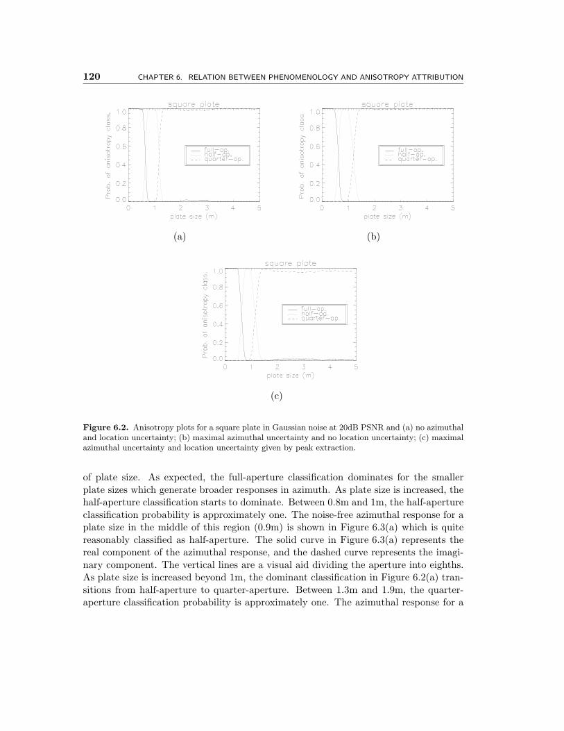
120 CHAPTER 6. RELATION BETWEEN PHENOMENOLOGY AND ANISOTROPY ATTRIBUTION
(a) (b)
(c)
Figure 6.2. Anisotropy plots for a square plate in Gaussian noise at 20dB PSNR and (a) no azimuthaland location uncertainty; (b) maximal azimuthal uncertainty and no location uncertainty; (c) maximalazimuthal uncertainty and location uncertainty given by peak extraction.
of plate size. As expected, the full-aperture classification dominates for the smallerplate sizes which generate broader responses in azimuth. As plate size is increased, thehalf-aperture classification starts to dominate. Between 0.8m and 1m, the half-apertureclassification probability is approximately one. The noise-free azimuthal response for aplate size in the middle of this region (0.9m) is shown in Figure 6.3(a) which is quitereasonably classified as half-aperture. The solid curve in Figure 6.3(a) represents thereal component of the azimuthal response, and the dashed curve represents the imagi-nary component. The vertical lines are a visual aid dividing the aperture into eighths.As plate size is increased beyond 1m, the dominant classification in Figure 6.2(a) tran-sitions from half-aperture to quarter-aperture. Between 1.3m and 1.9m, the quarter-aperture classification probability is approximately one. The azimuthal response for a
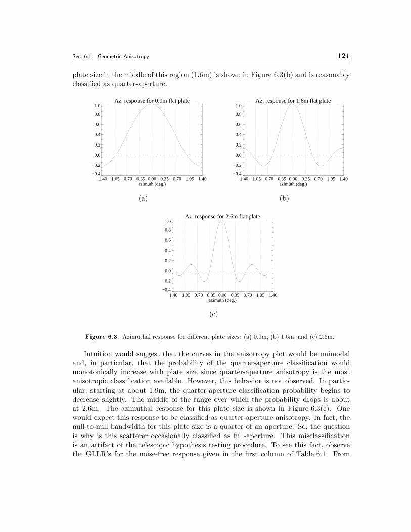
Sec. 6.1. Geometric Anisotropy 121
plate size in the middle of this region (1.6m) is shown in Figure 6.3(b) and is reasonablyclassified as quarter-aperture.
Az. response for 0.9m flat plate
−1.40−1.05−0.70−0.35 0.00 0.35 0.70 1.05 1.40azimuth (deg.)
−0.4
−0.2
0.0
0.2
0.4
0.6
0.8
1.0Az. response for 1.6m flat plate
−1.40 −1.05 −0.70 −0.35 0.00 0.35 0.70 1.05 1.40azimuth (deg.)
−0.4
−0.2
0.0
0.2
0.4
0.6
0.8
1.0
(a) (b)
Az. response for 2.6m flat plate
−1.40 −1.05 −0.70 −0.35 0.00 0.35 0.70 1.05 1.40azimuth (deg.)
−0.4
−0.2
0.0
0.2
0.4
0.6
0.8
1.0
(c)
Figure 6.3. Azimuthal response for different plate sizes: (a) 0.9m, (b) 1.6m, and (c) 2.6m.
Intuition would suggest that the curves in the anisotropy plot would be unimodaland, in particular, that the probability of the quarter-aperture classification wouldmonotonically increase with plate size since quarter-aperture anisotropy is the mostanisotropic classification available. However, this behavior is not observed. In partic-ular, starting at about 1.9m, the quarter-aperture classification probability begins todecrease slightly. The middle of the range over which the probability drops is aboutat 2.6m. The azimuthal response for this plate size is shown in Figure 6.3(c). Onewould expect this response to be classified as quarter-aperture anisotropy. In fact, thenull-to-null bandwidth for this plate size is a quarter of an aperture. So, the questionis why is this scatterer occasionally classified as full-aperture. This misclassificationis an artifact of the telescopic hypothesis testing procedure. To see this fact, observethe GLLR’s for the noise-free response given in the first column of Table 6.1. From
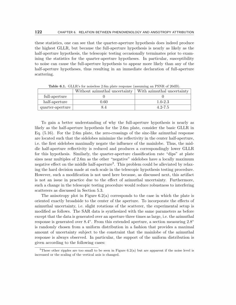
122 CHAPTER 6. RELATION BETWEEN PHENOMENOLOGY AND ANISOTROPY ATTRIBUTION
these statistics, one can see that the quarter-aperture hypothesis does indeed producethe highest GLLR, but because the full-aperture hypothesis is nearly as likely as thehalf-aperture hypothesis, the telescopic testing occasionally terminates prior to exam-ining the statistics for the quarter-aperture hypotheses. In particular, susceptibilityto noise can cause the full-aperture hypothesis to appear more likely than any of thehalf-aperture hypotheses, thus resulting in an immediate declaration of full-aperturescattering.
Table 6.1. GLLR’s for noiseless 2.6m plate response (assuming an PSNR of 20dB).
Without azimuthal uncertainty With azimuthal uncertaintyfull-aperture 0 0half-aperture 0.60 1.0-2.3
quarter-aperture 8.4 4.2-7.5
To gain a better understanding of why the full-aperture hypothesis is nearly aslikely as the half-aperture hypothesis for the 2.6m plate, consider the basic GLLR inEq. (5.16). For the 2.6m plate, the zero-crossings of the sinc-like azimuthal responseare located such that the sidelobes minimize the reflectivity in the center half-aperture,i.e. the first sidelobes maximally negate the influence of the mainlobe. Thus, the mid-dle half-aperture reflectivity is reduced and produces a correspondingly lower GLLRfor this hypothesis. Similarly, the quarter-aperture classification rate “dips” at platesizes near multiples of 2.6m as the other “negative” sidelobes have a locally maximumnegative effect on the middle half-aperture3. This problem could be alleviated by relax-ing the hard decision made at each scale in the telescopic hypothesis testing procedure.However, such a modification is not used here because, as discussed next, this artifactis not an issue in practice due to the effect of azimuthal uncertainty. Furthermore,such a change in the telescopic testing procedure would reduce robustness to interferingscatterers as discussed in Section 5.3.
The anisotropy plot in Figure 6.2(a) corresponds to the case in which the plate isoriented exactly broadside to the center of the aperture. To incorporate the effects ofazimuthal uncertainty, i.e. slight rotations of the scatterer, the experimental setup ismodified as follows. The SAR data is synthesized with the same parameters as beforeexcept that the data is generated over an aperture three times as large, i.e. the azimuthalresponse is generated over 8.4◦. From this extended aperture, a section measuring 2.8◦
is randomly chosen from a uniform distribution in a fashion that provides a maximalamount of uncertainty subject to the constraint that the mainlobe of the azimuthalresponse is always observed. In particular, the support of the uniform distribution isgiven according to the following cases:
3These other ripples are too small to be seen in Figure 6.2(a) but are apparent if the noise level isincreased or the scaling of the vertical axis is changed.
Sec. 6.1. Geometric Anisotropy 123
• if the plate size is less than two wavelengths (i.e. the plate size is less than 6.25cm), then the scatterer is considered isotropic and any 2.8◦ section of the extendedaperture can be selected,
• if the plate size is larger than two wavelengths but still small enough such thatthe half-power bandwidth of the azimuthal response is larger than 2.8◦, then anysection of the extended aperture within the half-power band can be chosen, and
• if the plate size is sufficiently large such that the half-power bandwidth of theazimuthal response is smaller than 2.8◦, then any section of the extended aperturecontaining the half-power band can be chosen.
The anisotropy plot incorporating this azimuthal uncertainty is shown in Figure 6.2(b).Interestingly, performance is improved for larger plate sizes by the addition of azimuthaluncertainty. In particular, the “dip” at 2.6m in Figure 6.2(a) is reduced. Looking at theGLLR’s in the second column of Table 6.1 for the 2.6m plate (assuming 20dB PSNR), itis apparent that it is not that the quarter-aperture GLLR increases (in fact, the GLLRdecreases slightly to typically vary between 4.2 and 7.5) but that the half-apertureGLLR increases to typically vary between 1.0 and 2.3. This increase occurs becausethe exact broadside orientation represents a worst-case scenario for the half-aperturehypothesis (relative to the full-aperture hypothesis) due to the maximal negative ef-fect that the first (and other odd number) sidelobes have on the middle half-aperturereflectivity. Azimuthal uncertainty, however, perturbs this degenerate alignment.
In addition to azimuthal uncertainty, the effect of location uncertainty can also beincorporated into the anisotropy plot. In particular, location uncertainty is simulatedby synthesizing a response for a random location and then using a peak extractionprocedure to determine the location to be used in the anisotropy test. Modeling lo-cation uncertainty in this fashion closely mimics the location uncertainty which arisesin peak-based ATR algorithms[25, 34, 13, 9, 23]. The anisotropy plot incorporatingboth azimuthal and location uncertainty is shown in Figure 6.2(c). Not surprisingly,there is a slight degradation in performance, particularly for larger plate sizes. Thisdegradation is due to the fact that large plates span several resolution cells over whichthe reflectivity is approximately constant. Thus, the peak extraction is susceptible tonoise over these resolution cells and frequently reports a location that, while on thescatterer, does not correspond to the scattering center. The resulting peak locationerror introduces a modulation on the observed azimuthal response which distorts theanisotropy classification4. In particular, for larger apertures, the linear phase on theazimuthal response prevents the sub-aperture reflectivity estimates from reaching theirtrue value due to the destructive interference that occurs when integrating over thesub-apertures. Thus, the energy from larger sub-apertures is biased towards smaller
4One might choose to model this location error as a nuisance parameter and address the error witha statistical approach. We do not, however, take this course due to the difficulties involved with thenonlinear effects the error has on the observed response. We thus view location error as an artifact ofthe peak-extraction algorithm and leave the problem for the peak-extraction to address.
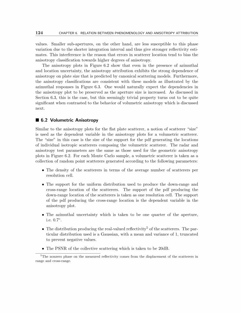
124 CHAPTER 6. RELATION BETWEEN PHENOMENOLOGY AND ANISOTROPY ATTRIBUTION
values. Smaller sub-apertures, on the other hand, are less susceptible to this phasevariation due to the shorter integration interval and thus give stronger reflectivity esti-mates. This interference is the reason that errors in scatterer location tend to bias theanisotropy classification towards higher degrees of anisotropy.
The anisotropy plots in Figure 6.2 show that even in the presence of azimuthaland location uncertainty, the anisotropy attribution exhibits the strong dependence ofanisotropy on plate size that is predicted by canonical scattering models. Furthermore,the anisotropy classifications are consistent with these models as illustrated by theazimuthal responses in Figure 6.3. One would naturally expect the dependencies inthe anisotropy plot to be preserved as the aperture size is increased. As discussed inSection 6.3, this is the case, but this seemingly trivial property turns out to be quitesignificant when contrasted to the behavior of volumetric anisotropy which is discussednext.
� 6.2 Volumetric Anisotropy
Similar to the anisotropy plots for the flat plate scatterer, a notion of scatterer “size”is used as the dependent variable in the anisotropy plots for a volumetric scatterer.The “size” in this case is the size of the support for the pdf generating the locationsof individual isotropic scatterers composing the volumetric scatterer. The radar andanisotropy test parameters are the same as those used for the geometric anisotropyplots in Figure 6.2. For each Monte Carlo sample, a volumetric scatterer is taken as acollection of random point scatterers generated according to the following parameters:
• The density of the scatterers in terms of the average number of scatterers perresolution cell.
• The support for the uniform distribution used to produce the down-range andcross-range location of the scatterers. The support of the pdf producing thedown-range location of the scatterers is taken as one resolution cell. The supportof the pdf producing the cross-range location is the dependent variable in theanisotropy plot.
• The azimuthal uncertainty which is taken to be one quarter of the aperture,i.e. 0.7◦.
• The distribution producing the real-valued reflectivity5 of the scatterers. The par-ticular distribution used is a Gaussian, with a mean and variance of 1, truncatedto prevent negative values.
• The PSNR of the collective scattering which is taken to be 20dB.5The nonzero phase on the measured reflectivity comes from the displacement of the scatterers in
range and cross-range.
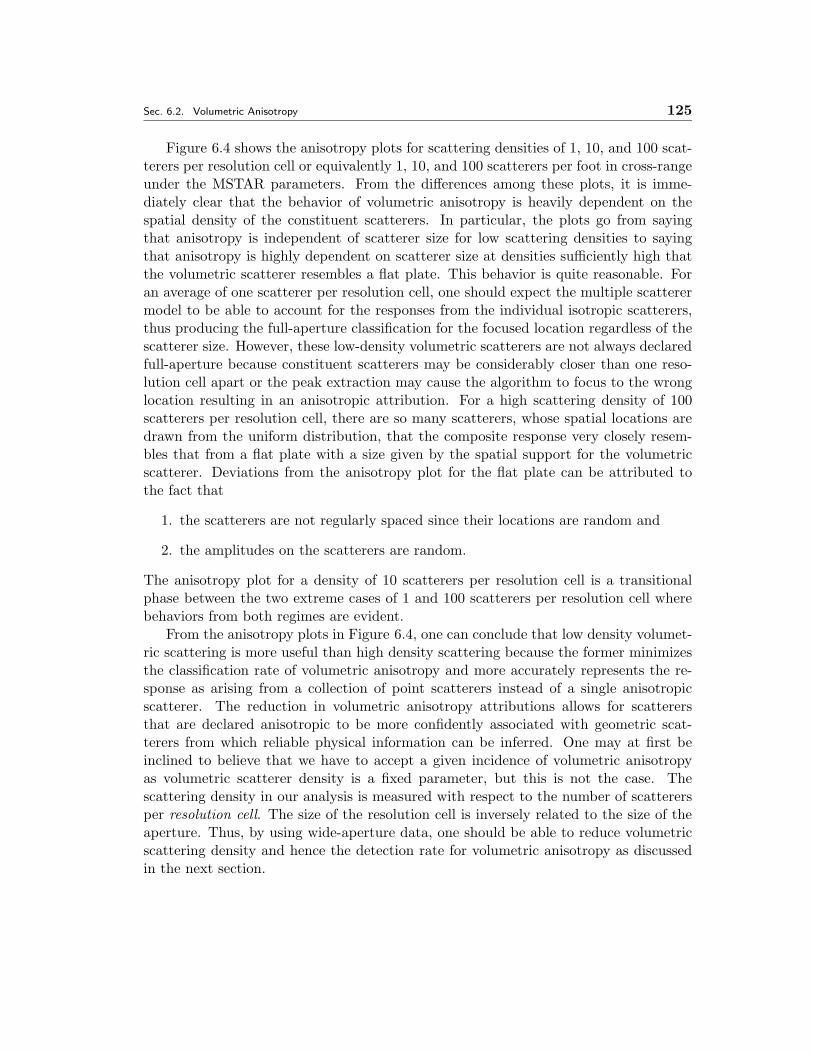
Sec. 6.2. Volumetric Anisotropy 125
Figure 6.4 shows the anisotropy plots for scattering densities of 1, 10, and 100 scat-terers per resolution cell or equivalently 1, 10, and 100 scatterers per foot in cross-rangeunder the MSTAR parameters. From the differences among these plots, it is imme-diately clear that the behavior of volumetric anisotropy is heavily dependent on thespatial density of the constituent scatterers. In particular, the plots go from sayingthat anisotropy is independent of scatterer size for low scattering densities to sayingthat anisotropy is highly dependent on scatterer size at densities sufficiently high thatthe volumetric scatterer resembles a flat plate. This behavior is quite reasonable. Foran average of one scatterer per resolution cell, one should expect the multiple scatterermodel to be able to account for the responses from the individual isotropic scatterers,thus producing the full-aperture classification for the focused location regardless of thescatterer size. However, these low-density volumetric scatterers are not always declaredfull-aperture because constituent scatterers may be considerably closer than one reso-lution cell apart or the peak extraction may cause the algorithm to focus to the wronglocation resulting in an anisotropic attribution. For a high scattering density of 100scatterers per resolution cell, there are so many scatterers, whose spatial locations aredrawn from the uniform distribution, that the composite response very closely resem-bles that from a flat plate with a size given by the spatial support for the volumetricscatterer. Deviations from the anisotropy plot for the flat plate can be attributed tothe fact that
1. the scatterers are not regularly spaced since their locations are random and
2. the amplitudes on the scatterers are random.
The anisotropy plot for a density of 10 scatterers per resolution cell is a transitionalphase between the two extreme cases of 1 and 100 scatterers per resolution cell wherebehaviors from both regimes are evident.
From the anisotropy plots in Figure 6.4, one can conclude that low density volumet-ric scattering is more useful than high density scattering because the former minimizesthe classification rate of volumetric anisotropy and more accurately represents the re-sponse as arising from a collection of point scatterers instead of a single anisotropicscatterer. The reduction in volumetric anisotropy attributions allows for scatterersthat are declared anisotropic to be more confidently associated with geometric scat-terers from which reliable physical information can be inferred. One may at first beinclined to believe that we have to accept a given incidence of volumetric anisotropyas volumetric scatterer density is a fixed parameter, but this is not the case. Thescattering density in our analysis is measured with respect to the number of scatterersper resolution cell. The size of the resolution cell is inversely related to the size of theaperture. Thus, by using wide-aperture data, one should be able to reduce volumetricscattering density and hence the detection rate for volumetric anisotropy as discussedin the next section.
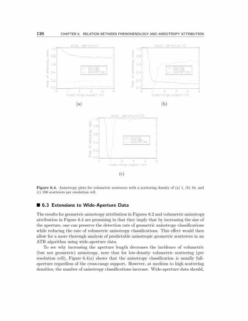
126 CHAPTER 6. RELATION BETWEEN PHENOMENOLOGY AND ANISOTROPY ATTRIBUTION
(a) (b)
(c)
Figure 6.4. Anisotropy plots for volumetric scatterers with a scattering density of (a) 1, (b) 10, and(c) 100 scatterers per resolution cell.
� 6.3 Extensions to Wide-Aperture Data
The results for geometric anisotropy attribution in Figures 6.2 and volumetric anisotropyattribution in Figure 6.4 are promising in that they imply that by increasing the size ofthe aperture, one can preserve the detection rate of geometric anisotropy classificationswhile reducing the rate of volumetric anisotropy classifications. This effect would thenallow for a more thorough analysis of predictable anisotropic geometric scatterers in anATR algorithm using wide-aperture data.
To see why increasing the aperture length decreases the incidence of volumetric(but not geometric) anisotropy, note that for low-density volumetric scattering (perresolution cell), Figure 6.4(a) shows that the anisotropy classification is usually full-aperture regardless of the cross-range support. However, at medium to high scatteringdensities, the number of anisotropy classifications increase. Wide-aperture data should,
Sec. 6.3. Extensions to Wide-Aperture Data 127
thus, reduce the number of anisotropy classifications because the larger aperture reducesthe scattering density in terms of the number of scatterers per resolution cell. Forexample, increasing the aperture size by a factor of ten decreases the resolution cellsize and hence scattering density by the same factor. From the anisotropy plots inFigure 6.4, it is apparent that such a factor should have a significant impact on the rateof volumetric anisotropy classifications. Geometric scatterers, on the other hand, canbe considered to be composed of a continuum of infinitely small scatterers (with respectto practical imaging resolutions), so increasing the resolution by an order of magnitude,or more, does not detract from the high scatterer density thus preserving the structureof the anisotropy plot.
The above is an image (or spatial) domain explanation for why wide-aperture datawould reduce the rate of volumetric anisotropy while preserving that of geometricanisotropy. There is an additional azimuthal domain interpretation. Consider a scat-terer that is declared anisotropic based on narrow-aperture data. This classification ismade because most of the energy is concentrated in one region of the aperture. Increas-ing the aperture length, however, increases the range over which the azimuthal responseis observed. For a volumetric scatterer, there is likely to be a considerable energy con-tribution in the newly added sections of the aperture because the underlying responseis not truly unimodal as depicted in Figure 6.1(b). However, a geometric scatterer witha unimodal azimuthal response should have little energy in the newly added aperturesections due to the these measurements capturing the tails of the azimuthal response.Furthermore, many anisotropic geometric scatterers exhibit sinc-like oscillations in thetails of their response (which nearly integrate to zero in the sub-apertures) while manyvolumetric scatterers do not. Thus, for volumetric scatterers, there is likely to be con-siderable energy in newly appended aperture sections which may change the anisotropyclassification, but for geometric scatterers, the newly appended aperture sections willcontain little energy thereby leaving the anisotropy attribution unchanged.
To verify this conjecture empirically, anisotropy plots for the geometric and volumet-ric scatterers are generated in the same fashion as before except that the aperture sizeis increased by a factor of eight. This modification naturally changes the sub-aperturepyramid used. To be consistent with the narrow-aperture results, we use a four-level,half-overlapping, half-aperture pyramid which consists of
• the 22.4◦ full-aperture at scale 0,
• 2.8◦ 1/8th-apertures at scale 1,
• 1.4◦ 1/16th-apertures at scale 2, and
• 0.7◦ 1/32th-apertures at scale 3.
Furthermore, again for consistency, the 22.4◦ full-aperture classification is not allowedto be declared in the anisotropy attribution process as this degree of anisotropy is not
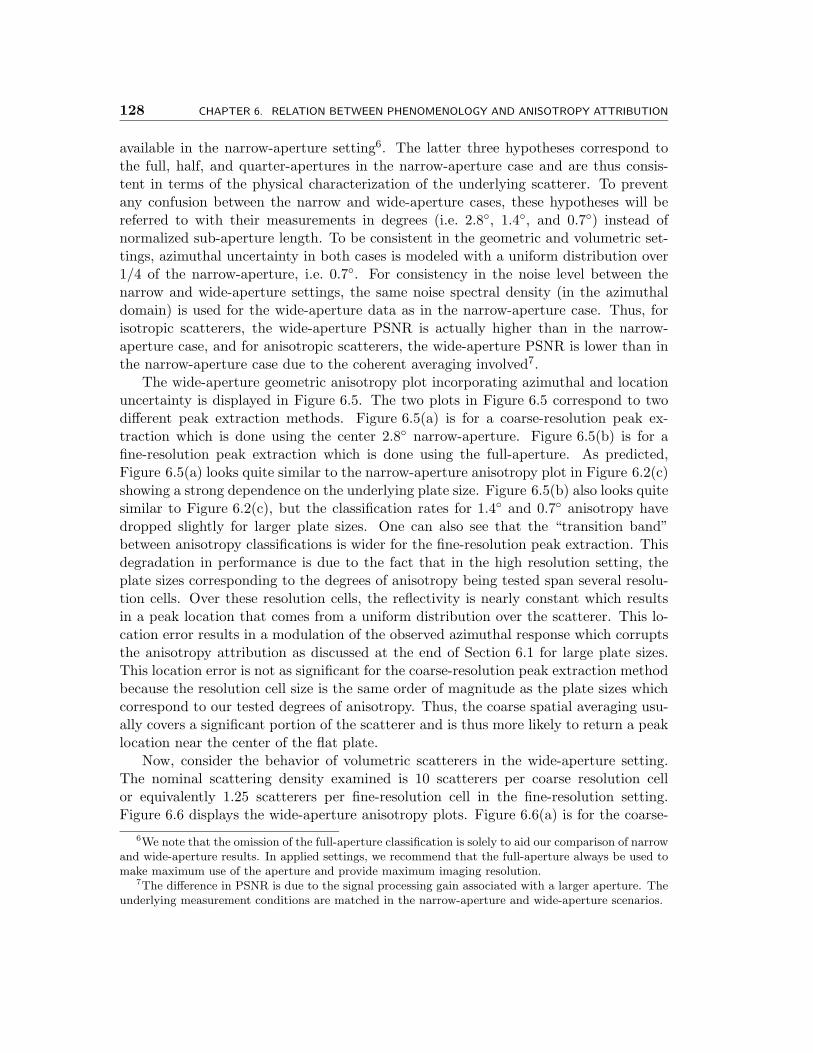
128 CHAPTER 6. RELATION BETWEEN PHENOMENOLOGY AND ANISOTROPY ATTRIBUTION
available in the narrow-aperture setting6. The latter three hypotheses correspond tothe full, half, and quarter-apertures in the narrow-aperture case and are thus consis-tent in terms of the physical characterization of the underlying scatterer. To preventany confusion between the narrow and wide-aperture cases, these hypotheses will bereferred to with their measurements in degrees (i.e. 2.8◦, 1.4◦, and 0.7◦) instead ofnormalized sub-aperture length. To be consistent in the geometric and volumetric set-tings, azimuthal uncertainty in both cases is modeled with a uniform distribution over1/4 of the narrow-aperture, i.e. 0.7◦. For consistency in the noise level between thenarrow and wide-aperture settings, the same noise spectral density (in the azimuthaldomain) is used for the wide-aperture data as in the narrow-aperture case. Thus, forisotropic scatterers, the wide-aperture PSNR is actually higher than in the narrow-aperture case, and for anisotropic scatterers, the wide-aperture PSNR is lower than inthe narrow-aperture case due to the coherent averaging involved7.
The wide-aperture geometric anisotropy plot incorporating azimuthal and locationuncertainty is displayed in Figure 6.5. The two plots in Figure 6.5 correspond to twodifferent peak extraction methods. Figure 6.5(a) is for a coarse-resolution peak ex-traction which is done using the center 2.8◦ narrow-aperture. Figure 6.5(b) is for afine-resolution peak extraction which is done using the full-aperture. As predicted,Figure 6.5(a) looks quite similar to the narrow-aperture anisotropy plot in Figure 6.2(c)showing a strong dependence on the underlying plate size. Figure 6.5(b) also looks quitesimilar to Figure 6.2(c), but the classification rates for 1.4◦ and 0.7◦ anisotropy havedropped slightly for larger plate sizes. One can also see that the “transition band”between anisotropy classifications is wider for the fine-resolution peak extraction. Thisdegradation in performance is due to the fact that in the high resolution setting, theplate sizes corresponding to the degrees of anisotropy being tested span several resolu-tion cells. Over these resolution cells, the reflectivity is nearly constant which resultsin a peak location that comes from a uniform distribution over the scatterer. This lo-cation error results in a modulation of the observed azimuthal response which corruptsthe anisotropy attribution as discussed at the end of Section 6.1 for large plate sizes.This location error is not as significant for the coarse-resolution peak extraction methodbecause the resolution cell size is the same order of magnitude as the plate sizes whichcorrespond to our tested degrees of anisotropy. Thus, the coarse spatial averaging usu-ally covers a significant portion of the scatterer and is thus more likely to return a peaklocation near the center of the flat plate.
Now, consider the behavior of volumetric scatterers in the wide-aperture setting.The nominal scattering density examined is 10 scatterers per coarse resolution cellor equivalently 1.25 scatterers per fine-resolution cell in the fine-resolution setting.Figure 6.6 displays the wide-aperture anisotropy plots. Figure 6.6(a) is for the coarse-
6We note that the omission of the full-aperture classification is solely to aid our comparison of narrowand wide-aperture results. In applied settings, we recommend that the full-aperture always be used tomake maximum use of the aperture and provide maximum imaging resolution.
7The difference in PSNR is due to the signal processing gain associated with a larger aperture. Theunderlying measurement conditions are matched in the narrow-aperture and wide-aperture scenarios.
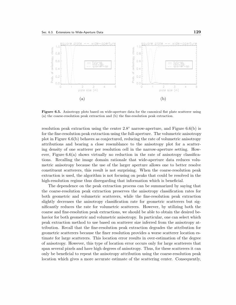
Sec. 6.3. Extensions to Wide-Aperture Data 129
(a) (b)
Figure 6.5. Anisotropy plots based on wide-aperture data for the canonical flat plate scatterer using(a) the coarse-resolution peak extraction and (b) the fine-resolution peak extraction.
resolution peak extraction using the center 2.8◦ narrow-aperture, and Figure 6.6(b) isfor the fine-resolution peak extraction using the full-aperture. The volumetric anisotropyplot in Figure 6.6(b) behaves as conjectured, reducing the rate of volumetric anisotropyattributions and bearing a close resemblance to the anisotropy plot for a scatter-ing density of one scatterer per resolution cell in the narrow-aperture setting. How-ever, Figure 6.6(a) shows virtually no reduction in the rate of anisotropy classifica-tions. Recalling the image domain rationale that wide-aperture data reduces volu-metric anisotropy because the use of the larger aperture allows one to better resolveconstituent scatterers, this result is not surprising. When the coarse-resolution peakextraction is used, the algorithm is not focusing on peaks that could be resolved in thehigh-resolution regime thus disregarding that information which is beneficial.
The dependence on the peak extraction process can be summarized by saying thatthe coarse-resolution peak extraction preserves the anisotropy classification rates forboth geometric and volumetric scatterers, while the fine-resolution peak extractionslightly decreases the anisotropy classification rate for geometric scatterers but sig-nificantly reduces the rate for volumetric scatterers. However, by utilizing both thecoarse and fine-resolution peak extractions, we should be able to obtain the desired be-havior for both geometric and volumetric anisotropy. In particular, one can select whichpeak extraction method to use based on scatterer size inferred from the anisotropy at-tribution. Recall that the fine-resolution peak extraction degrades the attribution forgeometric scatterers because the finer resolution provides a worse scatterer location es-timate for large scatterers. This location error results in over-estimation of the degreeof anisotropy. However, this type of location error occurs only for large scatterers thatspan several pixels and have high degrees of anisotropy. Thus, for these scatterers it canonly be beneficial to repeat the anisotropy attribution using the coarse-resolution peaklocation which gives a more accurate estimate of the scattering center. Consequently,
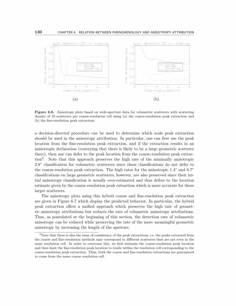
130 CHAPTER 6. RELATION BETWEEN PHENOMENOLOGY AND ANISOTROPY ATTRIBUTION
(a) (b)
Figure 6.6. Anisotropy plots based on wide-aperture data for volumetric scatterers with scatteringdensity of 10 scatterers per coarse-resolution cell using (a) the coarse-resolution peak extraction and(b) the fine-resolution peak extraction.
a decision-directed procedure can be used to determine which scale peak extractionshould be used in the anisotropy attribution. In particular, one can first use the peaklocation from the fine-resolution peak extraction, and if the extraction results in ananisotropic declaration (conveying that there is likely to be a large geometric scattererthere), then one can defer to the peak location from the coarse-resolution peak extrac-tion8. Note that this approach preserves the high rate of the minimally anisotropic2.8◦ classification for volumetric scatterers since these classifications do not defer tothe coarse-resolution peak extraction. The high rates for the anisotropic 1.4◦ and 0.7◦
classifications on large geometric scatterers, however, are also preserved since their ini-tial anisotropy classification is usually over-estimated and thus defers to the locationestimate given by the coarse-resolution peak extraction which is more accurate for theselarger scatterers.
The anisotropy plots using this hybrid coarse and fine-resolution peak extractionare given in Figure 6.7 which display the predicted behavior. In particular, the hybridpeak extraction offers a unified approach which preserves the high rate of geomet-ric anisotropy attributions but reduces the rate of volumetric anisotropy attributions.Thus, as postulated at the beginning of this section, the detection rate of volumetricanisotropy can be reduced while preserving the rate of the more meaningful geometricanisotropy by increasing the length of the aperture.
8Note that there is also the issue of consistency of the peak extractions, i.e. the peaks extracted fromthe coarse and fine-resolution methods may correspond to different scatterers that are not even in thesame resolution cell. In order to overcome this, we first estimate the coarse-resolution peak locationand then limit the fine-resolution peak location to reside within the resolution cell corresponding to thecoarse-resolution peak extraction. Thus, both the coarse and fine-resolution extractions are guaranteedto come from the same coarse resolution cell.
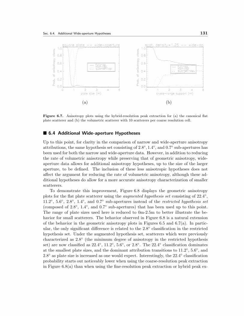
Sec. 6.4. Additional Wide-aperture Hypotheses 131
(a) (b)
Figure 6.7. Anisotropy plots using the hybrid-resolution peak extraction for (a) the canonical flatplate scatterer and (b) the volumetric scatterer with 10 scatterers per coarse resolution cell.
� 6.4 Additional Wide-aperture Hypotheses
Up to this point, for clarity in the comparison of narrow and wide-aperture anisotropyattributions, the same hypothesis set consisting of 2.8◦, 1.4◦, and 0.7◦ sub-apertures hasbeen used for both the narrow and wide-aperture data. However, in addition to reducingthe rate of volumetric anisotropy while preserving that of geometric anisotropy, wide-aperture data allows for additional anisotropy hypotheses, up to the size of the largeraperture, to be defined. The inclusion of these less anisotropic hypotheses does notaffect the argument for reducing the rate of volumetric anisotropy, although these ad-ditional hypotheses do allow for a more accurate anisotropy characterization of smallerscatterers.
To demonstrate this improvement, Figure 6.8 displays the geometric anisotropyplots for the flat plate scatterer using the augmented hypothesis set consisting of 22.4◦,11.2◦, 5.6◦, 2.8◦, 1.4◦, and 0.7◦ sub-apertures instead of the restricted hypothesis set(composed of 2.8◦, 1.4◦, and 0.7◦ sub-apertures) that has been used up to this point.The range of plate sizes used here is reduced to 0m-2.5m to better illustrate the be-havior for small scatterers. The behavior observed in Figure 6.8 is a natural extensionof the behavior in the geometric anisotropy plots in Figures 6.5 and 6.7(a). In partic-ular, the only significant difference is related to the 2.8◦ classification in the restrictedhypothesis set. Under the augmented hypothesis set, scatterers which were previouslycharacterized as 2.8◦ (the minimum degree of anisotropy in the restricted hypothesisset) are now classified as 22.4◦, 11.2◦, 5.6◦, or 2.8◦. The 22.4◦ classification dominatesat the smallest plate sizes, and the dominant attribution transitions to 11.2◦, 5.6◦, and2.8◦ as plate size is increased as one would expect. Interestingly, the 22.4◦ classificationprobability starts out noticeably lower when using the coarse-resolution peak extractionin Figure 6.8(a) than when using the fine-resolution peak extraction or hybrid peak ex-
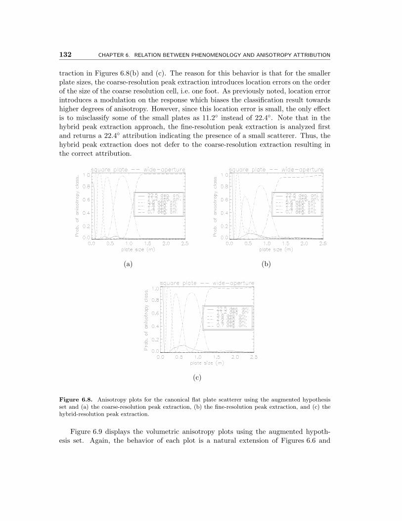
132 CHAPTER 6. RELATION BETWEEN PHENOMENOLOGY AND ANISOTROPY ATTRIBUTION
traction in Figures 6.8(b) and (c). The reason for this behavior is that for the smallerplate sizes, the coarse-resolution peak extraction introduces location errors on the orderof the size of the coarse resolution cell, i.e. one foot. As previously noted, location errorintroduces a modulation on the response which biases the classification result towardshigher degrees of anisotropy. However, since this location error is small, the only effectis to misclassify some of the small plates as 11.2◦ instead of 22.4◦. Note that in thehybrid peak extraction approach, the fine-resolution peak extraction is analyzed firstand returns a 22.4◦ attribution indicating the presence of a small scatterer. Thus, thehybrid peak extraction does not defer to the coarse-resolution extraction resulting inthe correct attribution.
(a) (b)
(c)
Figure 6.8. Anisotropy plots for the canonical flat plate scatterer using the augmented hypothesisset and (a) the coarse-resolution peak extraction, (b) the fine-resolution peak extraction, and (c) thehybrid-resolution peak extraction.
Figure 6.9 displays the volumetric anisotropy plots using the augmented hypoth-esis set. Again, the behavior of each plot is a natural extension of Figures 6.6 and
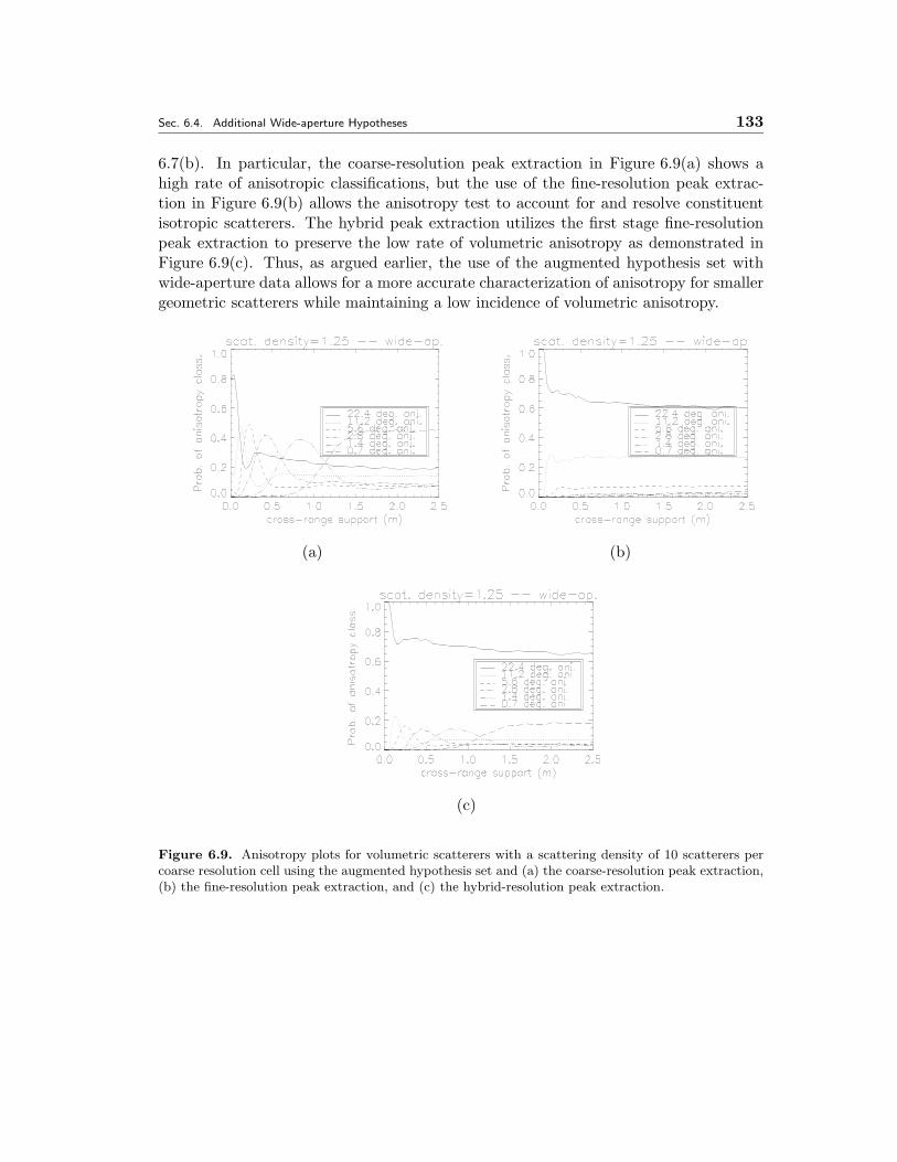
Sec. 6.4. Additional Wide-aperture Hypotheses 133
6.7(b). In particular, the coarse-resolution peak extraction in Figure 6.9(a) shows ahigh rate of anisotropic classifications, but the use of the fine-resolution peak extrac-tion in Figure 6.9(b) allows the anisotropy test to account for and resolve constituentisotropic scatterers. The hybrid peak extraction utilizes the first stage fine-resolutionpeak extraction to preserve the low rate of volumetric anisotropy as demonstrated inFigure 6.9(c). Thus, as argued earlier, the use of the augmented hypothesis set withwide-aperture data allows for a more accurate characterization of anisotropy for smallergeometric scatterers while maintaining a low incidence of volumetric anisotropy.
(a) (b)
(c)
Figure 6.9. Anisotropy plots for volumetric scatterers with a scattering density of 10 scatterers percoarse resolution cell using the augmented hypothesis set and (a) the coarse-resolution peak extraction,(b) the fine-resolution peak extraction, and (c) the hybrid-resolution peak extraction.
134 CHAPTER 6. RELATION BETWEEN PHENOMENOLOGY AND ANISOTROPY ATTRIBUTION
� 6.5 Wide-aperture GUS Data
This section applies the anisotropy attribution to peak scatterers extracted from themeasured wide-aperture Grayling Ultra-wideband SAR (GUS) data set. The data hasa resolution of 1.9 inches in down and cross-range achieved using a 4GHz bandwidth,a 10GHz center frequency, and a 26◦ aperture. For narrow-aperture comparisons, themiddle 3.3◦ section of this aperture (i.e. the middle eighth-aperture) is taken as thenarrow-aperture data. For each narrow-aperture peak extraction, the anisotropy test isapplied with the restricted hypothesis set composed of 3.3◦, 1.6◦, and 0.8◦ sub-apertureswhich correspond to the full, half, and quarter narrow-apertures. For the wide-aperturedata, the hybrid-resolution peak extraction method described in the previous sectionis used to determine peak locations. Because the wider aperture allows for moreanisotropy hypotheses to be defined, there are several choices for the hypothesis setin this regime. Two particular sets are examined. One choice is the restricted hypothe-sis set used in the narrow-aperture case. An alternative is the augmented hypothesis setobtained by taking all the sub-apertures in the half-overlapping, half-aperture pyramidfor the wide-aperture, i.e. the degrees of anisotropy in the augmented hypothesis setare {26◦, 13◦, 6.5◦, 3.3◦, 1.6◦, 0.8◦}. Figures 6.10 and 6.11 show the extracted peaks andtheir associated anisotropy attribution using the narrow and wide-aperture data for twodifferent vehicles. In (a) and (c) of each figure, the log-magnitude imagery obtainedusing the narrow and wide-apertures are displayed. In (b) and (d), the log-magnitudeimage is displayed again but with additional symbol overlays specifying the locationand anisotropy of each peak extraction. For the anisotropy attributions in (b) and (d),a black circle denotes 3.3◦ anisotropy, a square denotes 1.6◦ anisotropy, and a triangledenotes 0.8◦ anisotropy. To denote the additional wide-aperture 26◦, 13◦, and 6.5◦ at-tributions, we again use the circle, square, and triangle, respectively, but display themin white instead of black.
In each of the images, the peak extractions that are labeled as anisotropic arefrequently associated with an apparent geometric scatterer. In particular, the collectionslabeled “A” and “B” in Figure 6.10(d) appear to be large geometric scatterers and areappropriately characterized as anisotropic. Note that based on the narrow-aperturedata, the two scatterers labeled “A” are attributed as 3.3◦ in Figure 6.10(b), but thereare no means of telling if the underlying scatterers are actually 3.3◦ or perhaps lessanisotropic since 3.3◦ is the lowest degree of anisotropy available in the narrow-aperturesetting. However, using the augmented hypothesis set afforded by the wide-aperture,it is apparent that the degree of anisotropy for both scatterers is in fact approximately3.3◦, and not much more. This attribution is reasonable since the scatterers span severalresolution cells and appear geometric in nature in the high-resolution image. Thisexample demonstrates that the additional hypotheses afforded by the larger apertureallow more information about the scatterer anisotropy to be conveyed.
Another instance of large geometric scattering is the collection labeled “B” inFigure 6.10. These peak extractions appear to be associated with large flat geomet-ric scatterers, which are reflected in their anisotropy attributions most of which are
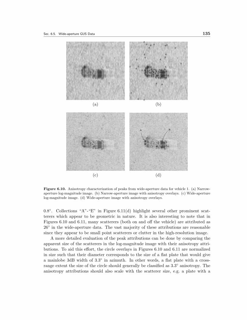
Sec. 6.5. Wide-aperture GUS Data 135
(a) (b)
A B
(c) (d)
Figure 6.10. Anisotropy characterization of peaks from wide-aperture data for vehicle 1. (a) Narrow-aperture log-magnitude image. (b) Narrow-aperture image with anisotropy overlays. (c) Wide-aperturelog-magnitude image. (d) Wide-aperture image with anisotropy overlays.
0.8◦. Collections “A”-“E” in Figure 6.11(d) highlight several other prominent scat-terers which appear to be geometric in nature. It is also interesting to note that inFigures 6.10 and 6.11, many scatterers (both on and off the vehicle) are attributed as26◦ in the wide-aperture data. The vast majority of these attributions are reasonablesince they appear to be small point scatterers or clutter in the high-resolution image.
A more detailed evaluation of the peak attributions can be done by comparing theapparent size of the scatterers in the log-magnitude image with their anisotropy attri-butions. To aid this effort, the circle overlays in Figures 6.10 and 6.11 are normalizedin size such that their diameter corresponds to the size of a flat plate that would givea mainlobe 3dB width of 3.3◦ in azimuth. In other words, a flat plate with a cross-range extent the size of the circle should generally be classified as 3.3◦ anisotropy. Theanisotropy attributions should also scale with the scatterer size, e.g. a plate with a
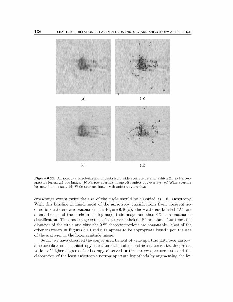
136 CHAPTER 6. RELATION BETWEEN PHENOMENOLOGY AND ANISOTROPY ATTRIBUTION
(a) (b)
EC
A
B
D
(c) (d)
Figure 6.11. Anisotropy characterization of peaks from wide-aperture data for vehicle 2. (a) Narrow-aperture log-magnitude image. (b) Narrow-aperture image with anisotropy overlays. (c) Wide-aperturelog-magnitude image. (d) Wide-aperture image with anisotropy overlays.
cross-range extent twice the size of the circle should be classified as 1.6◦ anisotropy.With this baseline in mind, most of the anisotropy classifications from apparent ge-ometric scatterers are reasonable. In Figure 6.10(d), the scatterers labeled “A” areabout the size of the circle in the log-magnitude image and thus 3.3◦ is a reasonableclassification. The cross-range extent of scatterers labeled “B” are about four times thediameter of the circle and thus the 0.8◦ characterizations are reasonable. Most of theother scatterers in Figures 6.10 and 6.11 appear to be appropriate based upon the sizeof the scatterer in the log-magnitude image.
So far, we have observed the conjectured benefit of wide-aperture data over narrow-aperture data on the anisotropy characterization of geometric scatterers, i.e. the preser-vation of higher degrees of anisotropy observed in the narrow-aperture data and theelaboration of the least anisotropic narrow-aperture hypothesis by augmenting the hy-
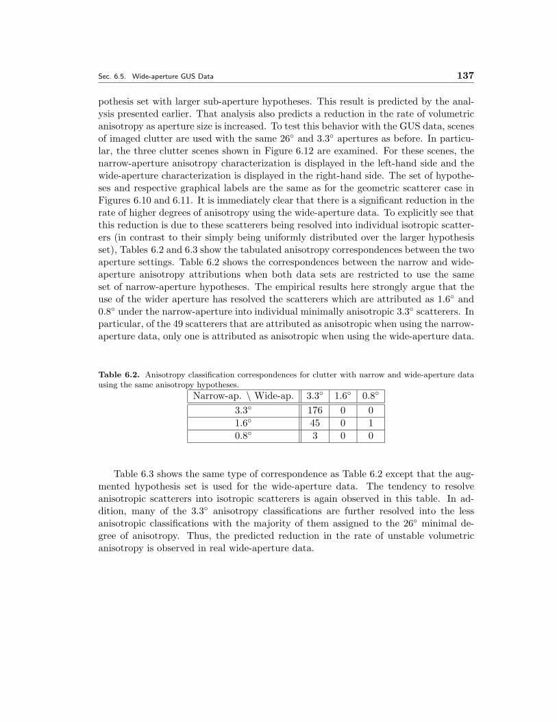
Sec. 6.5. Wide-aperture GUS Data 137
pothesis set with larger sub-aperture hypotheses. This result is predicted by the anal-ysis presented earlier. That analysis also predicts a reduction in the rate of volumetricanisotropy as aperture size is increased. To test this behavior with the GUS data, scenesof imaged clutter are used with the same 26◦ and 3.3◦ apertures as before. In particu-lar, the three clutter scenes shown in Figure 6.12 are examined. For these scenes, thenarrow-aperture anisotropy characterization is displayed in the left-hand side and thewide-aperture characterization is displayed in the right-hand side. The set of hypothe-ses and respective graphical labels are the same as for the geometric scatterer case inFigures 6.10 and 6.11. It is immediately clear that there is a significant reduction in therate of higher degrees of anisotropy using the wide-aperture data. To explicitly see thatthis reduction is due to these scatterers being resolved into individual isotropic scatter-ers (in contrast to their simply being uniformly distributed over the larger hypothesisset), Tables 6.2 and 6.3 show the tabulated anisotropy correspondences between the twoaperture settings. Table 6.2 shows the correspondences between the narrow and wide-aperture anisotropy attributions when both data sets are restricted to use the sameset of narrow-aperture hypotheses. The empirical results here strongly argue that theuse of the wider aperture has resolved the scatterers which are attributed as 1.6◦ and0.8◦ under the narrow-aperture into individual minimally anisotropic 3.3◦ scatterers. Inparticular, of the 49 scatterers that are attributed as anisotropic when using the narrow-aperture data, only one is attributed as anisotropic when using the wide-aperture data.
Table 6.2. Anisotropy classification correspondences for clutter with narrow and wide-aperture datausing the same anisotropy hypotheses.
Narrow-ap. \ Wide-ap. 3.3◦ 1.6◦ 0.8◦
3.3◦ 176 0 01.6◦ 45 0 10.8◦ 3 0 0
Table 6.3 shows the same type of correspondence as Table 6.2 except that the aug-mented hypothesis set is used for the wide-aperture data. The tendency to resolveanisotropic scatterers into isotropic scatterers is again observed in this table. In ad-dition, many of the 3.3◦ anisotropy classifications are further resolved into the lessanisotropic classifications with the majority of them assigned to the 26◦ minimal de-gree of anisotropy. Thus, the predicted reduction in the rate of unstable volumetricanisotropy is observed in real wide-aperture data.
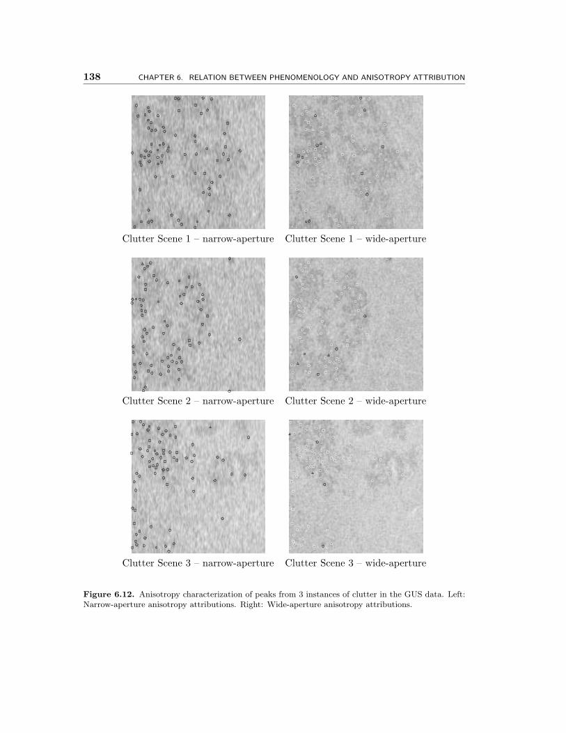
138 CHAPTER 6. RELATION BETWEEN PHENOMENOLOGY AND ANISOTROPY ATTRIBUTION
Clutter Scene 1 – narrow-aperture Clutter Scene 1 – wide-aperture
Clutter Scene 2 – narrow-aperture Clutter Scene 2 – wide-aperture
Clutter Scene 3 – narrow-aperture Clutter Scene 3 – wide-aperture
Figure 6.12. Anisotropy characterization of peaks from 3 instances of clutter in the GUS data. Left:Narrow-aperture anisotropy attributions. Right: Wide-aperture anisotropy attributions.
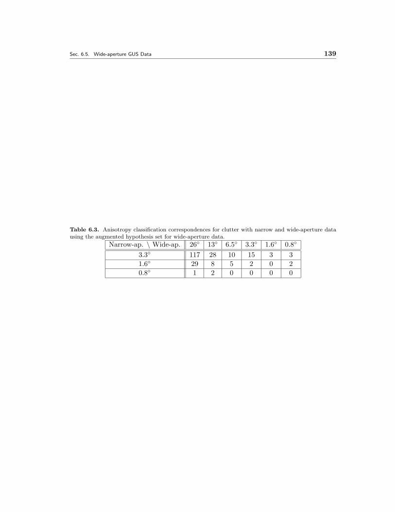
Sec. 6.5. Wide-aperture GUS Data 139
Table 6.3. Anisotropy classification correspondences for clutter with narrow and wide-aperture datausing the augmented hypothesis set for wide-aperture data.
Narrow-ap. \ Wide-ap. 26◦ 13◦ 6.5◦ 3.3◦ 1.6◦ 0.8◦
3.3◦ 117 28 10 15 3 31.6◦ 29 8 5 2 0 20.8◦ 1 2 0 0 0 0

140 CHAPTER 6. RELATION BETWEEN PHENOMENOLOGY AND ANISOTROPY ATTRIBUTION
Chapter 7
Iterative Anisotropy Attribution
In this chapter, we develop an enhanced, iterative algorithm for attributing anisotropyand estimating sub-aperture reflectivity. The idea behind this algorithm begins witha simple examination of the structure and limitations of the anisotropy attributionprocedure developed in Chapters 5 and used in Chapter 6. Specifically, that algo-rithm produces an anisotropy classification and a reflectivity estimate for each pixelby using a pyramid of sub-aperture reflectivity measurements. However, because thesesub-aperture measurements use only a fraction of the full-aperture, they have corre-spondingly coarser resolutions. These larger resolution cells allow the sub-aperturemeasurements to be corrupted by scatterers that are located within these larger cellsbut outside the finest resolution cell. This corruption from neighboring scatterers resultsin both a coarse imaging resolution and incorrect anisotropy attributions.
In Chapter 5, we described an approach to deal with this “nuisance” effect of inter-ference from scatterers in neighboring finest-resolution pixels. In particular, we consid-ered the estimation of anisotropy and reflectivity at a particular pixel (which we will re-fer to as the focused pixel). In processing the sub-aperture measurements correspondingto that focused pixel, we also included a set of additional unknown parameters corre-sponding to the reflectivities in an entire symmetric window of neighboring cross-range(finest-resolution) pixels. We then performed a generalized likelihood computation.This computation first estimates the reflectivities of the neighboring pixels in an MAPfashion. These estimates are then used to subtract out the effects of the interferingpixels in the anisotropy attribution of the focused pixel. As we will see, the approachdescribed in this chapter also performs a GLLR-based attribution and estimation butwith some differences to improve the modeling of neighboring scatterers.
The algorithm developed in Chapter 5, while producing very useful results, suffersfrom two potential inconsistencies. The first concerns the physical size of scatterers withhighly anisotropic attributions. In particular, suppose that a given focused pixel has ahighly anisotropic scatterer, i.e. the level of anisotropy indicates that the physical extentof the scatterer corresponds to several pixels (which we will call on-scatterer pixels) inthe finest-scale image. In this case, the reflectivities in these neighboring pixels are notnuisances since these pixels correspond to the same physical scatterer as the focusedpixel. Consequently, the GLLR approach of Chapter 5 erroneously subtracts out theeffects of these “neighbors”. The over-compensation for this single, physically large
141
142 CHAPTER 7. ITERATIVE ANISOTROPY ATTRIBUTION
scatterer distorts the estimation and attribution of the focused pixel. However, supposethat we have a preliminary estimate of attribution at all of these locations, e.g. byapplying the algorithm of Chapter 5. Perhaps the attributions of these neighboringpixels can be used to group the pixels into sets corresponding to individual scatterers in amanner that reflects the relationship between the degree of anisotropy and spatial extentof the scatterer. With such groupings, we can re-perform the anisotropy attribution ina manner that reduces this over-compensation, resulting in more accurate estimates ofreflectivity and anisotropy.
The other inconsistency in the algorithm used in Chapter 5 is the assumption thatthe “nuisance” contributions from neighboring pixels come from weak isotropic scatter-ers. Clearly, strong neighboring scatterers violate this assumption, but the assumptionis also violated by spatially extended, anisotropic scatterers that span several pixels.Contrary to the case of neighboring on-scatterer pixels, we do want to remove the ef-fects from these other locations, since these pixels correspond to a different scattererthan the focused pixel (and are hence called off-scatterer pixels). One way to do this,would be to take each grouping of off-scatterer pixels (corresponding to individual largescatterers) and subtract off their aggregate effect in a single step. Note that if we wereto subtract off the anisotropic effect for each individual pixel in this group, we wouldagain be over-compensating, since the anisotropy already captures the fact that theinfluence is from an extended scatterer spanning this group. However, an alternativethat does not over-compensate is to subtract the effect of each of the pixels in thatgrouping individually assuming that each of these neighbors is isotropic. While notrigorously the correct thing to do (since this approach neglects the phase consistencyacross the pixels due to the common underlying scatterer), this approach works well inpractice, as we will see.
The remainder of this chapter develops the iterative attribution algorithm and isorganized as follows. Section 7.1 provides a high-level description of the algorithm whichis based on an aggregation/re-attribution iteration step. Section 7.2 addresses the pixelaggregation task by posing it in a maximum likelihood framework. Section 7.3 thenextends the anisotropy test from Chapter 5 to utilize the information from the scattereraggregation to remove the effects of neighboring scatterers. Section 7.4 provides resultson synthesized and MSTAR data to demonstrate the improvement over the methodspresented in Chapter 5.
� 7.1 Algorithm Overview
Figure 7.1 describes the structure of the algorithm developed in this chapter. The al-gorithm is broken down into three processing stages. Inputs to each processing blockare denoted by inward pointing arrows. Arrows coming from the top designate mea-surement data that do not change as the algorithm progresses. Arrows coming fromthe left are inputs from another block’s output. Thus, these data vary as the iterationprogresses. Processing outputs are denoted by arrows leaving a block. Arrows pointing
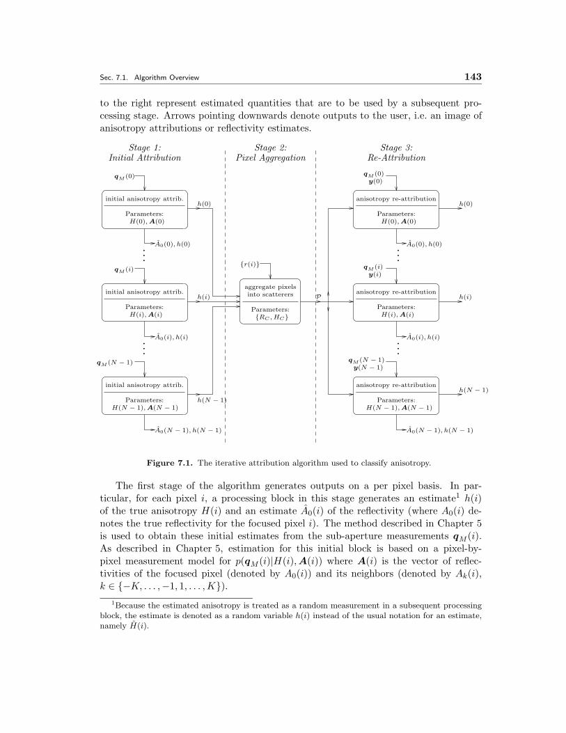
Sec. 7.1. Algorithm Overview 143
to the right represent estimated quantities that are to be used by a subsequent pro-cessing stage. Arrows pointing downwards denote outputs to the user, i.e. an image ofanisotropy attributions or reflectivity estimates.
initial anisotropy attrib.
Parameters:H(i), A(i)
A0(i), h(i)
qM (i)
..
.
..
.
..
.
..
.
initial anisotropy attrib.
Parameters:
A0(N − 1), h(N − 1)
qM (N − 1)
H(N − 1), A(N − 1)
aggregate pixelsinto scatterers
Parameters:
h(N − 1)
h(i)
{RC , HC}
h(0)
Parameters:H(i), A(i)
A0(i), h(i)
anisotropy re-attribution
Parameters:
A0(N − 1), h(N − 1)
anisotropy re-attribution
H(N − 1), A(N − 1)
h(0)
h(i)
Parameters:H(0), A(0)
A0(0), h(0)
anisotropy re-attribution
y(0)qM (0)
qM (i)y(i)
qM (N − 1)y(N − 1)
h(N − 1)
initial anisotropy attrib.
Parameters:H(0), A(0)
A0(0), h(0)
qM (0)
P
Stage 1:Initial Attribution Pixel Aggregation
Stage 3:Re-Attribution
Stage 2:
{r(i)}
Figure 7.1. The iterative attribution algorithm used to classify anisotropy.
The first stage of the algorithm generates outputs on a per pixel basis. In par-ticular, for each pixel i, a processing block in this stage generates an estimate1 h(i)of the true anisotropy H(i) and an estimate A0(i) of the reflectivity (where A0(i) de-notes the true reflectivity for the focused pixel i). The method described in Chapter 5is used to obtain these initial estimates from the sub-aperture measurements qM (i).As described in Chapter 5, estimation for this initial block is based on a pixel-by-pixel measurement model for p(qM (i)|H(i),A(i)) where A(i) is the vector of reflec-tivities of the focused pixel (denoted by A0(i)) and its neighbors (denoted by Ak(i),k ∈ {−K, . . . ,−1, 1, . . . ,K}).
1Because the estimated anisotropy is treated as a random measurement in a subsequent processingblock, the estimate is denoted as a random variable h(i) instead of the usual notation for an estimate,namely H(i).
144 CHAPTER 7. ITERATIVE ANISOTROPY ATTRIBUTION
The remaining two stages in Figure 7.1 correspond to an iterative refinement loopto be developed in the following two sections. The first of these two stages (i.e. thepixel aggregation step) takes the standard full-aperture estimates of log-magnitudereflectivity (denoted by r(i)) and current anisotropy estimates (denoted by h(i)) forevery pixel in the image and groups pixels so that each group corresponds to an estimateof a single, possibly physically-extended, scatterer. The result is a partition P groupingthe image pixels according to their underlying scatterers. The method we develop forthis aggregation step involves a Bayesian formulation that captures the fact that foreach cluster C of pixels corresponding to a single scatterer:
1. The log-magnitude full-aperture reflectivity estimates for each of the pixels inthe grouping should be statistically consistent with each other because thesereflectivities are all measurements of the single, physically-extended scatterer’slog-magnitude reflectivity RC .
2. The anisotropy classification for each of the pixels should be statistically consis-tent with each other as these attributions are all measurements of the scattereranisotropy HC .
3. The length of the grouping should be statistically consistent with the scattereranisotropy HC .
The Bayesian formulation we describe specifies a model p({r(i), h(i)}i∈C |RC , HC) cap-turing the characteristics for any hypothesized cluster C. Using a GLR philosophy, thisallows one to compute the most likely values of RC and HC for any hypothesized clusterand then to use these values in order to determine an approximation to the most likelypartition P of clusters.
The last stage in Figure 7.1 (i.e. the scatterer re-attribution step) refines the es-timates of anisotropy and reflectivity for each pixel i on a pixel-by-pixel basis. Eachprocessing block in this stage, takes as inputs:
• the groupings P just estimated in the scatterer aggregation step,
• the sub-aperture measurements qM (i), and
• the vector y(i) of full-aperture complex reflectivity measurements for the focusedpixel (denoted by y0(i)) and its neighbors at the finest resolution (denoted byyk(i), k ∈ {−K, . . . ,−1, 1, . . . ,K}).
These quantities are used to re-estimate scatterer anisotropy and reflectivity using amodified version of the algorithm in Chapter 5. The purpose of the modification isto avoid over-compensating for neighboring pixels that are part of the same scatterergrouping. In particular, in addition to using a measurement model for the observedsub-aperture reflectivities qM (i), we pose a measurement model for the observed finest-resolution complex reflectivities y(i). The underlying parameters (which we wish to
Sec. 7.2. Pixel Aggregation 145
estimate) in both of these models are the sub-aperture anisotropy H(i) and vectorof reflectivities A(i) as was the case in the initial attribution. The new observationy(i) replaces the zero-mean Gaussian prior on neighboring reflectivity estimates usedin Chapter 5 and leads to more accurate reflectivity estimates of the reflectivities inA(i). The segmentation is also used to aid the re-attribution by identifying on-scattererpixels and allowing their effects to be preserved, while allowing for the compensationof effects from interfering off-scatterer pixels. The anisotropy attributions that areproduced by this stage can be provided to the pixel aggregation block in the secondstage of Figure 7.1, thus starting another aggregation/re-attribution iteration.
� 7.2 Pixel Aggregation
The aggregation of image pixels into scatterers is the first phase of the two-stage it-eration. This section presents a maximum likelihood approach based on the inputmeasurements of pixel log-magnitude reflectivities2 and pixel anisotropy attributions.The goal of this stage is to produce a partition P of the pixels into a set of groupingscorresponding to scatterers. To achieve this goal, a measurement model is posed forthe cluster measurements {r(i)}i∈C and {h(i)}i∈C in any hypothesized cluster C con-ditioned on the unknown parameters RC and HC . It is then shown that the posedmodel produces a likelihood function that corresponds to an additive cost function.Consequently, the problem of finding the maximum likelihood partition becomes anoptimization problem on an additive cost function. An efficient, greedy algorithm isthen presented.
� 7.2.1 Problem Setup
We start by characterizing the relationship between (i) the anisotropy attributions h(i)and reflectivities r(i) that serve as the input data for the aggregation procedure and(ii) the unknown parameters HC and RC for any hypothesized cluster C. In particular,a Gaussian noise model is used for the reflectivities, i.e.
r(i) = RC + ui (7.1)
where ui ∼ N (0, ρ2r) and ρ2r is the variance on the reflectivities.The pixel-wise anisotropy attributions h(i) are modeled as identically distributed
samples given the underlying scatterer attribution. However, posing a reliable model forthe pixel anisotropy attributions is a difficult task. In particular, the confusion proba-bilities p(h(i)|HC) cannot be represented in closed form due to the manner in which theanisotropy attribution test partitions the observation space. Thus, we estimate theseprobabilities using Monte Carlo simulations. In particular, data are generated using
2For brevity, the term reflectivity will refer to the full-aperture log-magnitude reflectivity unlessotherwise specified for the remainder of this section.
146 CHAPTER 7. ITERATIVE ANISOTROPY ATTRIBUTION
the sub-aperture scattering model as described in Eq. (5.22), i.e.
qM = Ab(m, i) + w
where w ∼ N (0, 2(|A|2ρ2 + σ2)Λ). We will assume high SNR scattering which leads tothe approximation
w ∼ N (0, 2|A|2ρ2Λ).This approximation allows us to consider only the normalized case of A = 1 since thenoise standard deviation scales with the complex reflectivity A. The GLRT using thebasic GLLR statistic is then used to attribute each MC trial. The confusion probabilitiesp(h(i)
∣∣HC) are then taken as the relative frequency of occurrence in the MC trials andstored as a look-up table.
In addition to the pixel reflectivities r(i) and anisotropy attributions h(i), there is aninherent scatterer size conveyed by the grouping C. In particular, the cardinality #(C)of C specifies the number of pixels (and hence the spatial extent) for the scatterer.Recall from Section 2.1.3 that the image and azimuthal domains are related by theFourier transform. Thus, the cross-range extent of the scatterer is related to the degreeof anisotropy. In particular, because spatial and azimuthal concentration are inverselyrelated, the model for the observed scatterer size is defined in the azimuthal domain as
a(#(C)) = d(HC)(1 + v) (7.2)
where a(#(C)) is the 3dB width in the azimuthal domain of a flat plate of size #(C),d(HC) is the degree of anisotropy associated with HC , and v is noise with a double-exponential distribution. That Eq. (7.2) is not a deterministic relationship between sizeand anisotropy is due to the rudimentary nature of our characterization of anisotropy(e.g. many non-canonic responses can lead to the same level of anisotropy in our model).The multiplicative form of the model (leading to an error term proportional to the degreeof anisotropy) is consistent with the geometrically related lengths of the sub-aperturesin our model. The use of the double exponential model for v is for computationalconvenience. For reference, the model in Eq. (7.2) produces the likelihood
p (#(C)|d(HC)) =12ρl
exp
[−∣∣a(#(C))− d(HC)
∣∣ρl d(HC)
]. (7.3)
� 7.2.2 Aggregation Likelihood
In formulating the likelihood of an entire aggregation of pixels, we start by consideringa single cluster C. The likelihood of the data in this grouping is
p({r(i)}i∈C , {h(i)}i∈C∣∣RC , HC
)(7.4)
The models posed in the previous sub-section are used to decouple and simplify thislikelihood expression. First, note that although the individual pixel reflectivities r(i)
Sec. 7.2. Pixel Aggregation 147
are characterized by RC and the individual pixel anisotropy attributions h(i) are char-acterized by HC , the likelihood in Eq. (7.4) cannot immediately be written as a productof the terms p(r(i)|RC) and p(h(i)|HC). This cannot be done because the cardinality ofthe sets {r(i)}i∈C and {h(i)}i∈C are related to scatterer size. Consequently, considera-tion of the grouping introduces an additional dependency on the underlying anisotropy.However, by rewriting Eq. (7.4) to explicitly include the cardinality of C, we can obtainthe desired separation of terms. In particular, we can write
p({r(i)}i∈C , {h(i)}i∈C∣∣RC , HC
)= p
(#(C), {r(i)}i∈C , {h(i)}i∈C
∣∣RC , HC
)(7.5a)
= p(#(C)
∣∣RC , HC
)p({r(i)}i∈C , {h(i)}i∈C∣∣#(C), RC , HC
)(7.5b)
= p(#(C)
∣∣RC , HC
) ∏i∈C
p (r(i)|RC)∏i∈C
p (h(i)|HC) (7.5c)
= p(#(C)
∣∣d(HC)) ∏
i∈Cp (r(i)|RC)
∏i∈C
p (h(i)|HC) . (7.5d)
Eq. (7.5a) follows from the fact that #(C) is redundant in that can be determined from{r(i)}i∈C and {h(i)}i∈C . Eq. (7.5b) is an application of Bayes rule. Eq. (7.5c) followsfrom the fact that given RC , HC , and the size of the set C, we can model the r(i) andh(i) as i.i.d. Eq. (7.5d) follows from the degree of anisotropy characterizing the spatialextent of the scatterer.
With the likelihood specification from Eq. (7.5) in hand, we now proceed to developthe aggregation problem. We start with the simple case in which there are two pixelgroupings X and Y that neighbor each other, i.e. X ∪ Y is a connected set. For eachgrouping (X or Y ), it is known that all the pixels in that group correspond to thesame scatterer, i.e. X and Y each span part of a scatterer but not necessarily the entirescatterer. Based on the data r(i) and h(i), we wish to test whether X ∪ Y correspondsto a single scatterer (hypothesisG1) or separate scatterers (hypothesisG2). A maximumlikelihood test is used for this task.
Because the likelihood in Eq. (7.5) depends on the unknown parameters scattererreflectivity RC and anisotropy HC , these parameters are estimated and used to producea generalized likelihood. In particular, Eq. (7.1) is used to generate the ML estimateof RC , which is the sample mean of the reflectivities in group C. This estimate will bedenoted by RC . The ML estimate of HC is given by
HC = argmax(n,j)
{∏i∈C
p (h(i)|H = (n, j))
}. (7.6)
The probability models for the pixel reflectivity, pixel anisotropy, and cluster sizedefined in Section 7.2.1 can be inserted into Eq. (7.5) to determine the generalized likeli-hood of X and Y corresponding to two separate scatterers (G2) or X ∪ Y correspondingto a single scatterer (G1). In particular, the generalized likelihood of a group C (with
148 CHAPTER 7. ITERATIVE ANISOTROPY ATTRIBUTION
C representing X, Y , or X ∪ Y ) is
;C = p(#(C)
∣∣∣HC
) ∏i∈C
p(ri
∣∣∣RC
) ∏i∈C
p(h(i)
∣∣∣HC
)=
12ρl
exp
[−∣∣a(#(C))− d(HC)
∣∣ρl d(HC)
](2πρ2r)
−#(C)/2∏i∈C
exp
[(r(i)− RC)2
2ρ2r
] ∏i∈C
p(h(i)
∣∣∣HC
).
Thus, the GLLR between the two hypotheses G2 and G1 can be written as
γ = log(;X;Y;X∪Y
)= f(X ∪ Y )− f(X)− f(Y ) (7.7)
where f(C) is the negative log-likelihood for the data in set C. Note that the densitynormalization factor for the pixel reflectivities cancel in the likelihood ratio and canthus be omitted from the cost function, i.e.
f(C) = log(2ρl) +
∣∣a(#(C))− d(HC)∣∣
ρld(HC)+
12ρ2r
∑i∈C
(r(i)− RC)2 −∑i∈C
log(p(h(i)|HC
)).
(7.8)
Consequently, the decision on whether to merge the groupings X and Y is determinedby whether the costs of X and Y are lower individually (i.e. f(X)+ f(Y ) < f(X ∪ Y ))or the cost is lower by combining the two (i.e. f(X) + f(Y ) > f(X ∪ Y )).
The additive nature of the GLLR in Eq. (7.7) allows the aggregation rule easily tobe extended to consider an entire partition. In particular, assume that we are presentedwith two partitions P1 and P2 of all the cross-range pixels and that P2 is a refinementof P1, i.e. every C ∈ P1 can be partitioned by elements of P2. The task is then todetermine which partition has the higher generalized likelihood. The GLLR of thesetwo partitions can be written as
log
(∏C∈P2
;C∏C∈P1
;C
)= F (P1)− F (P2) (7.9)
where
F (P) =∑C∈P
f(C). (7.10)
Thus, the ML aggregation problem amounts to finding the partition with the minimumcost given by Eqs. (7.8) and (7.10)
� 7.2.3 Greedy Aggregation Algorithm
It is computationally prohibitive to evaluate the cost in Eq. (7.10) for every valid par-tition. Motivated by the additive structure of the cost in Eq. (7.10), we propose the
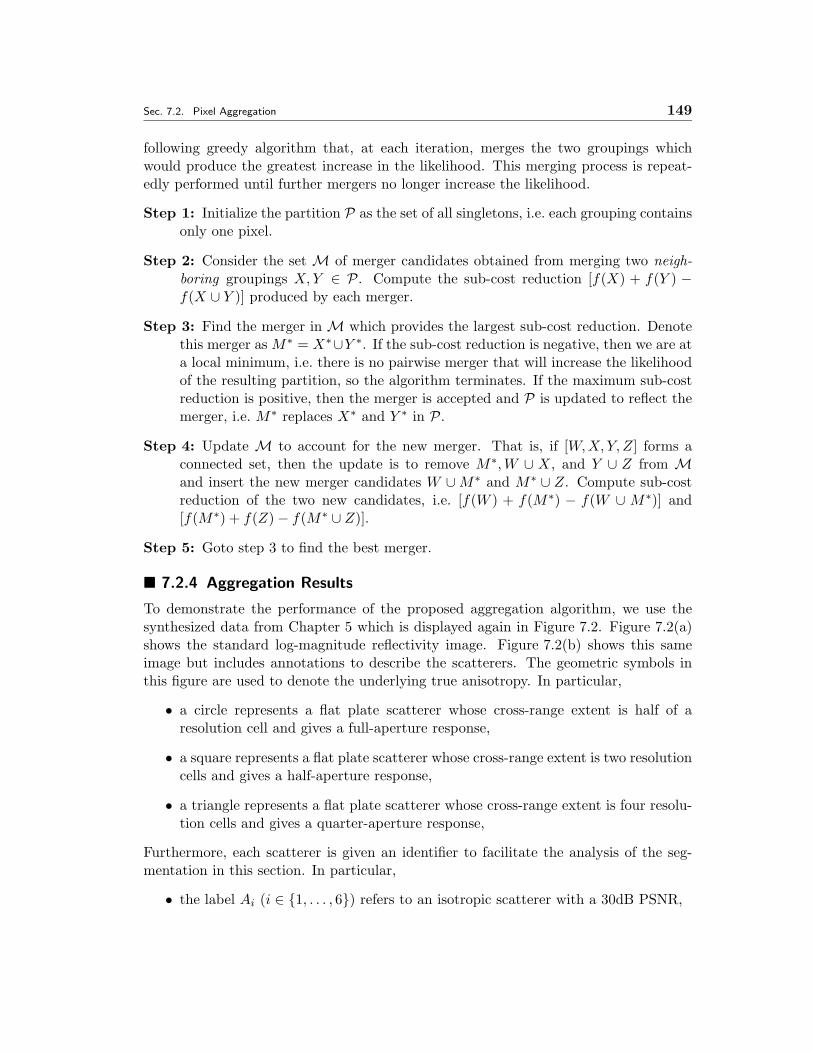
Sec. 7.2. Pixel Aggregation 149
following greedy algorithm that, at each iteration, merges the two groupings whichwould produce the greatest increase in the likelihood. This merging process is repeat-edly performed until further mergers no longer increase the likelihood.
Step 1: Initialize the partition P as the set of all singletons, i.e. each grouping containsonly one pixel.
Step 2: Consider the set M of merger candidates obtained from merging two neigh-boring groupings X,Y ∈ P. Compute the sub-cost reduction [f(X) + f(Y ) −f(X ∪ Y )] produced by each merger.
Step 3: Find the merger in M which provides the largest sub-cost reduction. Denotethis merger as M∗ = X∗∪Y ∗. If the sub-cost reduction is negative, then we are ata local minimum, i.e. there is no pairwise merger that will increase the likelihoodof the resulting partition, so the algorithm terminates. If the maximum sub-costreduction is positive, then the merger is accepted and P is updated to reflect themerger, i.e. M∗ replaces X∗ and Y ∗ in P.
Step 4: Update M to account for the new merger. That is, if [W,X, Y, Z] forms aconnected set, then the update is to remove M∗,W ∪ X, and Y ∪ Z from Mand insert the new merger candidates W ∪M∗ and M∗ ∪ Z. Compute sub-costreduction of the two new candidates, i.e. [f(W ) + f(M∗) − f(W ∪ M∗)] and[f(M∗) + f(Z)− f(M∗ ∪ Z)].
Step 5: Goto step 3 to find the best merger.
� 7.2.4 Aggregation Results
To demonstrate the performance of the proposed aggregation algorithm, we use thesynthesized data from Chapter 5 which is displayed again in Figure 7.2. Figure 7.2(a)shows the standard log-magnitude reflectivity image. Figure 7.2(b) shows this sameimage but includes annotations to describe the scatterers. The geometric symbols inthis figure are used to denote the underlying true anisotropy. In particular,
• a circle represents a flat plate scatterer whose cross-range extent is half of aresolution cell and gives a full-aperture response,
• a square represents a flat plate scatterer whose cross-range extent is two resolutioncells and gives a half-aperture response,
• a triangle represents a flat plate scatterer whose cross-range extent is four resolu-tion cells and gives a quarter-aperture response,
Furthermore, each scatterer is given an identifier to facilitate the analysis of the seg-mentation in this section. In particular,
• the label Ai (i ∈ {1, . . . , 6}) refers to an isotropic scatterer with a 30dB PSNR,
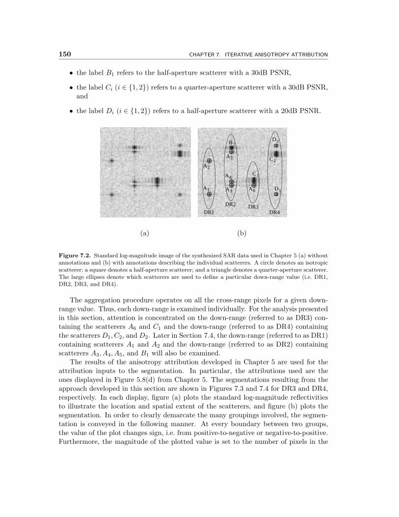
150 CHAPTER 7. ITERATIVE ANISOTROPY ATTRIBUTION
• the label B1 refers to the half-aperture scatterer with a 30dB PSNR,
• the label Ci (i ∈ {1, 2}) refers to a quarter-aperture scatterer with a 30dB PSNR,and
• the label Di (i ∈ {1, 2}) refers to a half-aperture scatterer with a 20dB PSNR.
1
C1
D1
DB
A2
A
2
A3
A
1
C2
A4
A6
5
DR1
DR2 DR3DR4
(a) (b)
Figure 7.2. Standard log-magnitude image of the synthesized SAR data used in Chapter 5 (a) withoutannotations and (b) with annotations describing the individual scatterers. A circle denotes an isotropicscatterer; a square denotes a half-aperture scatterer; and a triangle denotes a quarter-aperture scatterer.The large ellipses denote which scatterers are used to define a particular down-range value (i.e. DR1,DR2, DR3, and DR4).
The aggregation procedure operates on all the cross-range pixels for a given down-range value. Thus, each down-range is examined individually. For the analysis presentedin this section, attention is concentrated on the down-range (referred to as DR3) con-taining the scatterers A6 and C1 and the down-range (referred to as DR4) containingthe scatterersD1, C2, andD2. Later in Section 7.4, the down-range (referred to as DR1)containing scatterers A1 and A2 and the down-range (referred to as DR2) containingscatterers A3, A4, A5, and B1 will also be examined.
The results of the anisotropy attribution developed in Chapter 5 are used for theattribution inputs to the segmentation. In particular, the attributions used are theones displayed in Figure 5.8(d) from Chapter 5. The segmentations resulting from theapproach developed in this section are shown in Figures 7.3 and 7.4 for DR3 and DR4,respectively. In each display, figure (a) plots the standard log-magnitude reflectivitiesto illustrate the location and spatial extent of the scatterers, and figure (b) plots thesegmentation. In order to clearly demarcate the many groupings involved, the segmen-tation is conveyed in the following manner. At every boundary between two groups,the value of the plot changes sign, i.e. from positive-to-negative or negative-to-positive.Furthermore, the magnitude of the plotted value is set to the number of pixels in the
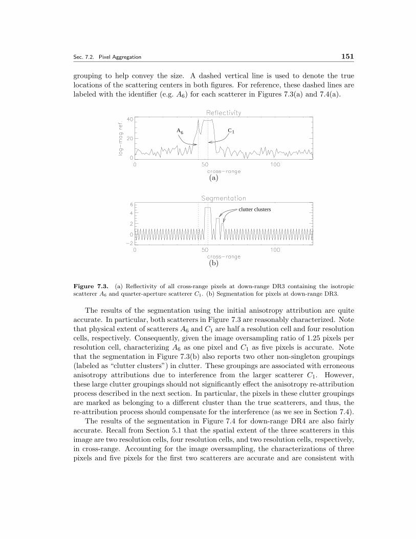
Sec. 7.2. Pixel Aggregation 151
grouping to help convey the size. A dashed vertical line is used to denote the truelocations of the scattering centers in both figures. For reference, these dashed lines arelabeled with the identifier (e.g. A6) for each scatterer in Figures 7.3(a) and 7.4(a).
6 C1A
(a)
clutter clusters
(b)
Figure 7.3. (a) Reflectivity of all cross-range pixels at down-range DR3 containing the isotropicscatterer A6 and quarter-aperture scatterer C1. (b) Segmentation for pixels at down-range DR3.
The results of the segmentation using the initial anisotropy attribution are quiteaccurate. In particular, both scatterers in Figure 7.3 are reasonably characterized. Notethat physical extent of scatterers A6 and C1 are half a resolution cell and four resolutioncells, respectively. Consequently, given the image oversampling ratio of 1.25 pixels perresolution cell, characterizing A6 as one pixel and C1 as five pixels is accurate. Notethat the segmentation in Figure 7.3(b) also reports two other non-singleton groupings(labeled as “clutter clusters”) in clutter. These groupings are associated with erroneousanisotropy attributions due to interference from the larger scatterer C1. However,these large clutter groupings should not significantly effect the anisotropy re-attributionprocess described in the next section. In particular, the pixels in these clutter groupingsare marked as belonging to a different cluster than the true scatterers, and thus, there-attribution process should compensate for the interference (as we see in Section 7.4).
The results of the segmentation in Figure 7.4 for down-range DR4 are also fairlyaccurate. Recall from Section 5.1 that the spatial extent of the three scatterers in thisimage are two resolution cells, four resolution cells, and two resolution cells, respectively,in cross-range. Accounting for the image oversampling, the characterizations of threepixels and five pixels for the first two scatterers are accurate and are consistent with
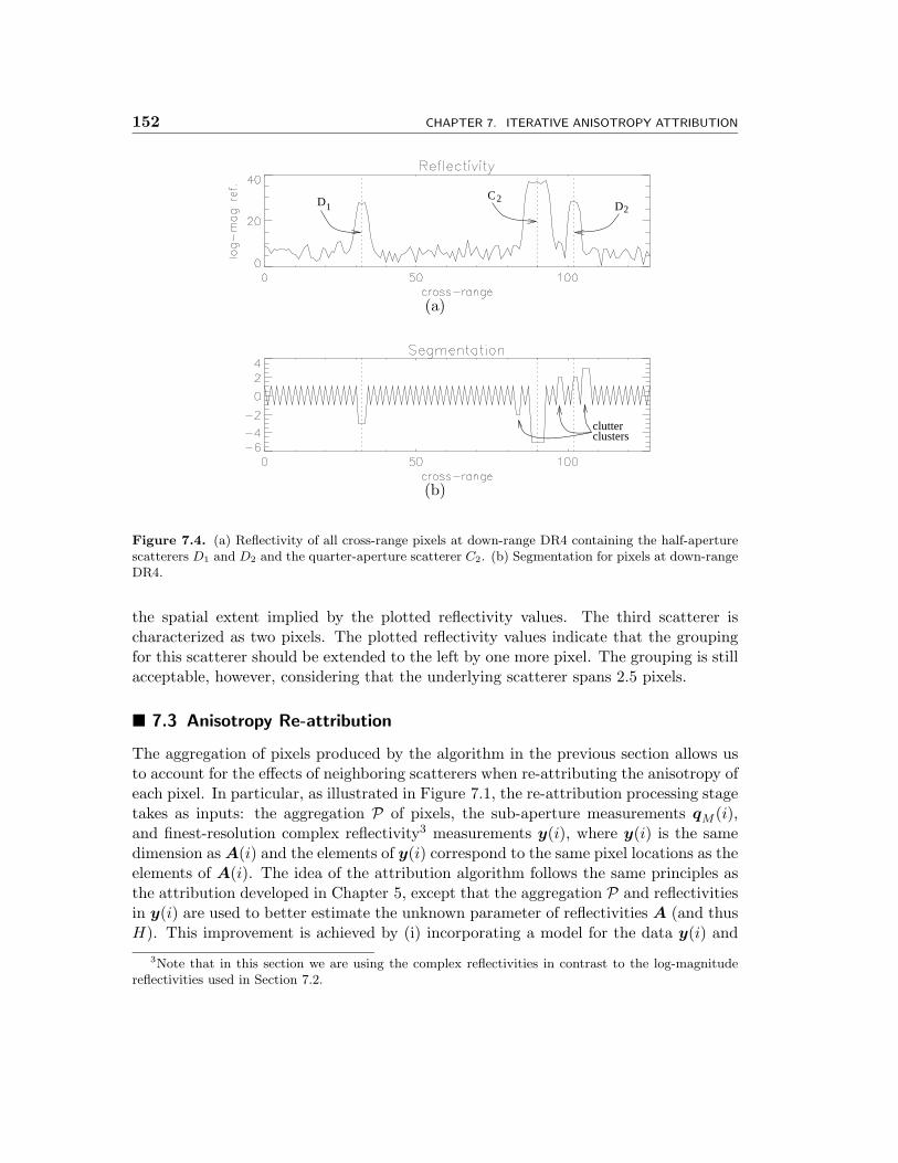
152 CHAPTER 7. ITERATIVE ANISOTROPY ATTRIBUTION
D1C2
D2
(a)
clutterclusters
(b)
Figure 7.4. (a) Reflectivity of all cross-range pixels at down-range DR4 containing the half-aperturescatterers D1 and D2 and the quarter-aperture scatterer C2. (b) Segmentation for pixels at down-rangeDR4.
the spatial extent implied by the plotted reflectivity values. The third scatterer ischaracterized as two pixels. The plotted reflectivity values indicate that the groupingfor this scatterer should be extended to the left by one more pixel. The grouping is stillacceptable, however, considering that the underlying scatterer spans 2.5 pixels.
� 7.3 Anisotropy Re-attribution
The aggregation of pixels produced by the algorithm in the previous section allows usto account for the effects of neighboring scatterers when re-attributing the anisotropy ofeach pixel. In particular, as illustrated in Figure 7.1, the re-attribution processing stagetakes as inputs: the aggregation P of pixels, the sub-aperture measurements qM (i),and finest-resolution complex reflectivity3 measurements y(i), where y(i) is the samedimension as A(i) and the elements of y(i) correspond to the same pixel locations as theelements of A(i). The idea of the attribution algorithm follows the same principles asthe attribution developed in Chapter 5, except that the aggregation P and reflectivitiesin y(i) are used to better estimate the unknown parameter of reflectivities A (and thusH). This improvement is achieved by (i) incorporating a model for the data y(i) and
3Note that in this section we are using the complex reflectivities in contrast to the log-magnitudereflectivities used in Section 7.2.
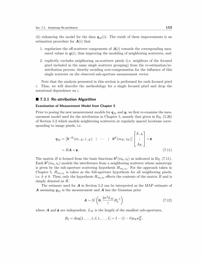
Sec. 7.3. Anisotropy Re-attribution 153
(ii) enhancing the model for the data qM (i). The result of these improvements is anestimation procedure for A(i) that
1. regularizes the off-scatterer components of A(i) towards the corresponding mea-sured values in y(i), thus improving the modeling of neighboring scatterers, and
2. explicitly excludes neighboring on-scatterer pixels (i.e. neighbors of the focusedpixel included in the same single scatterer grouping) from the re-estimation/re-attribution process, thereby avoiding over-compensation for the influence of thissingle scatterer on the observed sub-aperture measurement vector.
Note that the analysis presented in this section is performed for each focused pixeli. Thus, we will describe the methodology for a single focused pixel and drop thenotational dependence on i.
� 7.3.1 Re-attribution Algorithm
Examination of Measurement Model from Chapter 5
Prior to posing the new measurement models for qM and y, we first re-examine the mea-surement model used for the attribution in Chapter 5, namely that given in Eq. (5.26)of Section 5.2 which models neighboring scatterers at regularly spaced locations corre-sponding to image pixels, i.e.
qM =[b−K(m−K , i−K) | · · · | bK(mK , iK)
] A−K...
AK
+ εεε
= BA + εεε. (7.11)
The matrix B is formed from the basis functions bk(mk, ik) as indicated in Eq. (7.11).Each bk(mk, ik) models the interference from a neighboring scatterer whose anisotropyis given by the sub-aperture scattering hypothesis Hmk,ik . For the approach taken inChapter 5, Hmk,ik is taken as the full-aperture hypothesis for all neighboring pixels,i.e. k "= 0. Thus, only the hypothesis Hm0,i0 effects the contents of the matrix B and issimply denoted as H.
The estimate used for A in Section 5.2 can be interpreted as the MAP estimate ofA assuming qM is the measurement and A has the Gaussian prior
A ∼ N(0,
2σ2LM
γR−1
δ
)(7.12)
where A and εεε are independent, LM is the length of the smallest sub-apertures,
Rδ = diag[1, . . . , 1, δ, 1, . . . , 1] = I − (1− δ)eKeHK ,
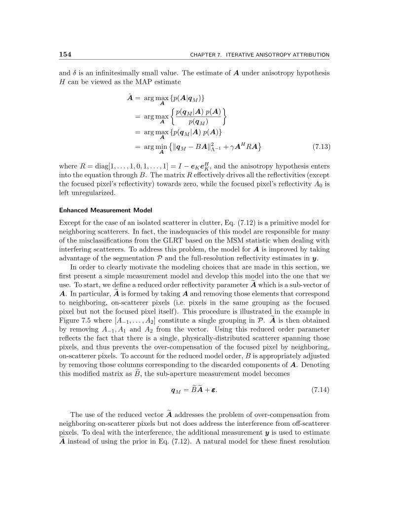
154 CHAPTER 7. ITERATIVE ANISOTROPY ATTRIBUTION
and δ is an infinitesimally small value. The estimate of A under anisotropy hypothesisH can be viewed as the MAP estimate
A = argmaxA
{p(A|qM )}
= argmaxA
{p(qM |A) p(A)
p(qM )
}= argmax
A{p(qM |A) p(A)}
= argminA
{‖qM −BA‖2Λ−1 + γAHRA}
(7.13)
where R = diag[1, . . . , 1, 0, 1, . . . , 1] = I − eKeHK , and the anisotropy hypothesis entersinto the equation through B. The matrix R effectively drives all the reflectivities (exceptthe focused pixel’s reflectivity) towards zero, while the focused pixel’s reflectivity A0 isleft unregularized.
Enhanced Measurement Model
Except for the case of an isolated scatterer in clutter, Eq. (7.12) is a primitive model forneighboring scatterers. In fact, the inadequacies of this model are responsible for manyof the misclassifications from the GLRT based on the MSM statistic when dealing withinterfering scatterers. To address this problem, the model for A is improved by takingadvantage of the segmentation P and the full-resolution reflectivity estimates in y.
In order to clearly motivate the modeling choices that are made in this section, wefirst present a simple measurement model and develop this model into the one that weuse. To start, we define a reduced order reflectivity parameter A which is a sub-vector ofA. In particular, A is formed by taking A and removing those elements that correspondto neighboring, on-scatterer pixels (i.e. pixels in the same grouping as the focusedpixel but not the focused pixel itself). This procedure is illustrated in the example inFigure 7.5 where [A−1, . . . , A2] constitute a single grouping in P. A is then obtainedby removing A−1, A1 and A2 from the vector. Using this reduced order parameterreflects the fact that there is a single, physically-distributed scatterer spanning thosepixels, and thus prevents the over-compensation of the focused pixel by neighboring,on-scatterer pixels. To account for the reduced model order, B is appropriately adjustedby removing those columns corresponding to the discarded components of A. Denotingthis modified matrix as B, the sub-aperture measurement model becomes
qM = BA + εεε. (7.14)
The use of the reduced vector A addresses the problem of over-compensation fromneighboring on-scatterer pixels but not does address the interference from off-scattererpixels. To deal with the interference, the additional measurement y is used to estimateA instead of using the prior in Eq. (7.12). A natural model for these finest resolution
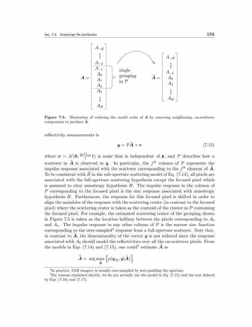
Sec. 7.3. Anisotropy Re-attribution 155
...
...
...
...
singlegroupingin P A = A0
A−2
A−K
A3
AK
A−K
A−2
A−1
A =A0
A1
A2
A3
AK
Figure 7.5. Illustration of reducing the model order of A by removing neighboring, on-scatterercomponents to produce A.
reflectivity measurements is
y = P A + v (7.15)
where v ∼ N (0, 2σ2LMγ I) is noise that is independent of εεε, and P describes how a
scatterer in A is observed in y. In particular, the jth column of P represents theimpulse response associated with the scatterer corresponding to the jth element of A.To be consistent with B in the sub-aperture scattering model of Eq. (7.14), all pixels areassociated with the full-aperture scattering hypothesis except the focused pixel whichis assumed to obey anisotropy hypothesis H. The impulse response in the column ofP corresponding to the focused pixel is the sinc response associated with anisotropyhypothesis H. Furthermore, the response for this focused pixel is shifted in order toalign the mainlobe of the response with the scattering center (in contrast to the focusedpixel) where the scattering center is taken as the centroid of the cluster in P containingthe focused pixel. For example, the estimated scattering center of the grouping shownin Figure 7.5 is taken as the location halfway between the pixels corresponding to A0
and A1. The impulse response in any other column of P is the narrow sinc functioncorresponding to the over-sampled4 response from a full-aperture scatterer. Note that,in contrast to A, the dimensionality of the vector y is not reduced since the responseassociated with A0 should model the reflectivities over all the on-scatterer pixels. Fromthe models in Eqs. (7.14) and (7.15), one could5 estimate A as
ˆA = argmax
A
{p(qM ,y|A)
}4In practice, SAR imagery is usually over-sampled by zero-padding the aperture.5For reasons explained shortly, we do not actually use the model in Eq. (7.15) and the test defined
by Eqs. (7.16) and (7.17).
156 CHAPTER 7. ITERATIVE ANISOTROPY ATTRIBUTION
= argmaxA
{p(qM |A)p(y|A)
}= argmin
A
{‖qM − BA‖2Λ−1 + γ‖y − P A‖2
}=[BHΛ−1B + γPHP
]−1 (BHΛ−1qM + γPHy
). (7.16)
This estimate of A could then be used to compute the error-norm
‖εεε‖2Λ−1 = ‖qM − BˆA‖2Λ−1 (7.17)
to determine a generalized likelihood of each sub-aperture hypothesis. These generalizedlikelihoods can then be used to perform a GLRT to characterize anisotropy.
The model in Eq. (7.15) accurately models the reflectivities in A under the correcthypothesis, but not under the incorrect hypothesis. Such behavior is not surprisingand is not a fundamental drawback. However, this behavior does severely impact theperformance of the anisotropy test if a telescopic hypothesis testing procedure is used.In particular, for a highly anisotropic scatterer, decision errors are made in the earlystages of the telescopic testing sequence that prevent the correct anisotropy hypothesisfrom being tested. This problem is best illustrated with an example. Consider thesituation illustrated in Figure 7.6 where a large, distributed scatterer is being modeledwith an insufficiently anisotropic response (i.e. one using too large of a sub-aperture).The location of the focused pixel in this figure is labeled with a “×” on the horizontalaxis. In order to match the finest resolution reflectivity for that location with anill-fitting sinc function, the estimate A0 is regularized towards a large negative valuesince we are focused on a negative sidelobe. Using such a poorly regularized value ofA in Eq. (7.17) produces large erratic error values for εεε under incorrect sub-aperturehypotheses. Thus, in the early stages of the telescopic test (when none of the examinedhypotheses are correct) the telescopic testing procedure frequently makes an “incorrect”decision in the sense that the decision either terminates the testing (having decided thatthe correct sub-aperture has been reached) or leads the telescopic testing proceduredown an incorrect path on the pyramid where the correct hypothesis is never evaluated.
We mention two methods to address this problem. One approach would be to omitthe telescopic testing procedure and evaluate all the sub-aperture hypotheses since theproblem only arises when the incorrect sub-aperture hypothesis is evaluated. Thiscourse is not taken in this thesis due to the computational savings the telescopic testingprocedure provides. Instead, the approach taken in this section is along the same linesas the approach in Section 5.2 where the reflectivity for the scatterer under examinationis left unregularized. The approach taken here uses the measurement y only to estimatethe reflectivity of neighboring scatterers and leaves the estimation of the focused pixel’sreflectivity to be determined by the sub-aperture measurements qM . In particular,the dimensionality of the measurement y is reduced by discarding all measurements
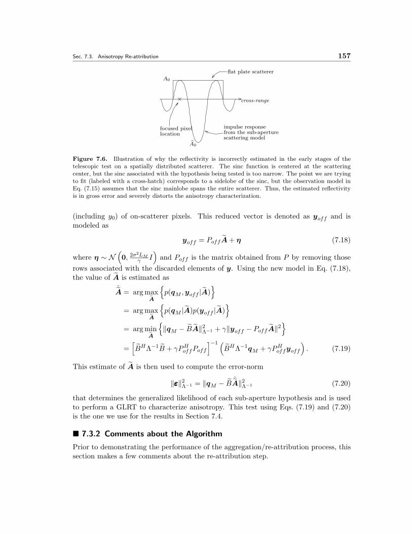
Sec. 7.3. Anisotropy Re-attribution 157
A0
A0
flat plate scatterer
from the sub-aperturescattering model
impulse responsefocused pixellocation
cross-range
Figure 7.6. Illustration of why the reflectivity is incorrectly estimated in the early stages of thetelescopic test on a spatially distributed scatterer. The sinc function is centered at the scatteringcenter, but the sinc associated with the hypothesis being tested is too narrow. The point we are tryingto fit (labeled with a cross-hatch) corresponds to a sidelobe of the sinc, but the observation model inEq. (7.15) assumes that the sinc mainlobe spans the entire scatterer. Thus, the estimated reflectivityis in gross error and severely distorts the anisotropy characterization.
(including y0) of on-scatterer pixels. This reduced vector is denoted as yoff and ismodeled as
yoff = PoffA + η (7.18)
where η ∼ N(0, 2σ
2LMγ I
)and Poff is the matrix obtained from P by removing those
rows associated with the discarded elements of y. Using the new model in Eq. (7.18),the value of A is estimated as
ˆA = argmax
A
{p(qM ,yoff |A)
}= argmax
A
{p(qM |A)p(yoff |A)
}= argmin
A
{‖qM − BA‖2Λ−1 + γ‖yoff − PoffA‖2
}=[BHΛ−1B + γPH
offPoff
]−1 (BHΛ−1qM + γPH
offyoff
). (7.19)
This estimate of A is then used to compute the error-norm
‖εεε‖2Λ−1 = ‖qM − BˆA‖2Λ−1 (7.20)
that determines the generalized likelihood of each sub-aperture hypothesis and is usedto perform a GLRT to characterize anisotropy. This test using Eqs. (7.19) and (7.20)is the one we use for the results in Section 7.4.
� 7.3.2 Comments about the Algorithm
Prior to demonstrating the performance of the aggregation/re-attribution process, thissection makes a few comments about the re-attribution step.
158 CHAPTER 7. ITERATIVE ANISOTROPY ATTRIBUTION
Modeling Neighbors as Isotropic
The first point we address is whether modeling neighboring scatterers as isotropic cap-tures the interference from anisotropic interfering scatterers. In particular, a single,physically-distributed scatterer exhibits a consistent phase on the reflectivity over theon-scatterer pixels. Although the approach presented in this section does not explicitlymodel this phase consistency, the estimate in Eq. (7.19) is still able to capture thisphase consistency to a large degree. In particular, this phase consistency is captured bythe measured complex reflectivities, albeit corrupted by measurement noise. Thus, forscatterers with a high SNR, there should be a strong (although not perfect) consistencyin the phase on the estimates of A corresponding to a single scatterer. The successof this approach in capturing the behavior of interfering scatterers is demonstrated inSection 7.4.
Omission of the Previous Iteration’s Anisotropy Estimates
The re-attribution statistic obtained from Eqs. (7.19) and (7.20) uses only the aggre-gated groupings, the full-aperture reflectivity measurements, and the sub-aperture re-flectivity measurements to estimate the anisotropy of a given pixel. Each neighboringscatterer is modeled as a series of isotropic scatterers instead of a single anisotropicscatterer because this pixel-wise approach is robust to attribution errors from earlieriterations. If a previous iteration’s anisotropy attribution and sub-aperture reflectiv-ity estimate are used to model neighboring scatterers, then initial attribution errorscould be catastrophic. In particular, consider the false anisotropy attributions in clut-ter around a strong scatterer. We will call these misclassifications phantom attributionsas the anisotropy attribution is due to the interference from a neighboring scatterer andnot the contents of the focused pixel’s resolution cell. Many of the sub-aperture reflec-tivity estimates for these phantom classifications are large because the associated coarseresolution cell contains part of the interfering scatterer. If these erroneous attributionsand reflectivity estimates are used in a re-attribution step, then the algorithm wouldcompensate for a non-existent scatterer which would almost surely lead to other errors.The re-attribution approach proposed in this chapter, however, is robust to such er-rors since the finest resolution reflectivities are used and the response from neighboringscatterers are modeled in a pixel-wise fashion. Because the finest resolution reflectiv-ities are used, one does not suffer from the coarser resolution associated with smallsub-apertures. Furthermore, because the scatterers are modeled pixel-by-pixel, the re-attribution step need only be able to distinguish on-scatterer from off-scatterer pixels,i.e. it is not necessary to determine the spatial extent of each interfering scatterer.
Skipping the Re-attribution Step
We also point out that the re-attribution for a pixel needs to be performed onlyif the grouping containing that pixel has changed from the previous aggregation/re-attribution iteration. In particular, if the set of on-scatterer pixels for a given location
Sec. 7.4. Experimental Results 159
is unchanged from the previous iteration, then all the quantities in Eqs. (7.19) and(7.20) are unchanged and the re-attribution can be skipped. We have observed that inpractice, the vast majority of pixels need to be re-attributed only once, i.e. after theinitial aggregation step. This is especially the case for clutter pixels which are usuallygrouped as singletons.
Independence of εεε and η
The observation models in Eqs. (7.14) and (7.18) assume that the noises εεε and v onthe sub-aperture and finest-resolution reflectivity measurements are independent. Thisassumption is not precisely true since the sub-aperture measurements qM and reflectiv-ities yoff are obtained from the same set of azimuthal data. However, we believe thatany existing dependencies are weak due to the differences in the way the measurementsare obtained. In particular,
• For the sub-aperture measurements, the azimuthal data is demodulated to focuson a particular pixel location. Then, the components of qM are obtained byintegrating this single azimuthal response over each individual sub-aperture.
• For the finest-resolution reflectivities, an azimuthal response is calculated for eachpixel location where the demodulation of the response varies according to thefocused location. Each of these multiple azimuthal responses are then integratedover the entire aperture to produce the set of reflectivities yoff .
Thus, the dependence (conditioned on A) between the two measurements should besmall because of the different modulations used prior to the integration and the differentintegration intervals used.
� 7.4 Experimental Results
This section demonstrates the results of the iterative anisotropy attribution. The algo-rithm is applied to the synthesized data used in Chapter 5 and the MSTAR data imagedat cardinal angles. The results on synthesized data are presented first to present a de-tailed analysis of the workings of the algorithm. The results on MSTAR data are thenpresented to demonstrate that the algorithm performs well in real-world settings.
For all the results in this section, the initial anisotropy attribution in stage 1 ofFigure 7.1 uses the GLRT based on the MSM statistic of Section 5.2 with the telescopictesting procedure and the same testing parameters as in Chapter 5. The segmentationparameters are taken as ρl = 0.5 and ρr = 0.5. The re-attribution parameters are takento be the same as in the initial attribution except for the regularization parameter whichis now taken to be γ = 0.25. The value of γ is reduced from 0.5 for the initial anisotropyattribution to 0.25 for the re-attribution in order to produce a consistent model for thesub-aperture and finest resolution reflectivity measurements. In particular, recall thatthe error η for the finest resolution reflectivities in Eq. (7.18) specifies the noise variance
160 CHAPTER 7. ITERATIVE ANISOTROPY ATTRIBUTION
as 2σ2LMγ Q−1
δ in order to produce the objective function in Eq. (7.19). Furthermore,recall from Eq. (5.5) that the noise variance on the full-aperture reflectivity estimate is2σ2. Thus, in order for these two models to be consistent, it must follow that
2σ2LM
γ= 2σ2
γ =1
LM= 0.25
for the three-level, half-overlapping, half-aperture pyramid. The larger value of γ = 0.5is necessary for the initial anisotropy attribution in order to suppress the contributionfrom other on-scatterer pixels. The re-attribution approach, however, already explic-itly removes these redundant parameters from the model, and thus, the regularizationparameter need not be set artificially high.
Figures 7.7 through 7.11 display the results of the iterative anisotropy attribution forthe synthetic image data used in Chapter 5 which is repeated in Figure 7.2. Figure 7.7displays the anisotropy attribution and sub-aperture reflectivity images at each itera-tion. Figures 7.7(a) and (b) are the result of the initial attribution using the GLRTbased on the MSM statistic of Section 5.2. Figures 7.7(c) through (f) are the resultsof the first and second re-attribution iterations. Subsequent aggregation/re-attributioniterations do not result in any changes from the attributions shown in figures (e) and(f). The improvement of the anisotropy re-attribution over the initial attribution isclear. The most obvious result is that all of the phantom attributions in clutter havebeen removed6 in Figures 7.7(c) and (e). In particular, the initial attribution in figure(a) produces several spurious anisotropic classifications in the vicinity of the annotatedscatterers. However, the aggregation/re-attribution corrects for all of these phantom at-tributions. The attribution of these clutter pixels as full-aperture by the re-attributionprocedure is achieved through the accurate modeling of the interference from the neigh-boring scatterers. The only criticism of the results in Figure 7.7 is that the attributionsof the pixels on the half-aperture scatterers (scatterers B1, D1, and D2 in Figure 7.2)are not all correct. In particular, while the scattering center for each scatterer is cor-rectly attributed as half-aperture (as marked by the square annotation in Figures 7.7(c)and (e), some of the pixels neighboring the scattering center are attributed incorrectlyas quarter-aperture (as indicated by their darker shading). These misclassifications aredue to location error. In particular, as described in Section 6.1, the displacement fromthe scattering center produces a modulation on the observed azimuthal response whichbiases the measured energy of larger sub-apertures towards zero, and thus, biases theanisotropy characterization towards more highly anisotropic attributions.
To examine the workings of the re-attribution in further detail, Figures 7.8 through7.11 display the segmentations produced for down-range locations DR1 through DR4in Figure 7.2. For each of the displays, figure (a) shows the standard, full-aperture,log-magnitude reflectivity. Figures (b) through (d) show the segmentation based on
6Note that a pre-screening threshold is not used for these results.
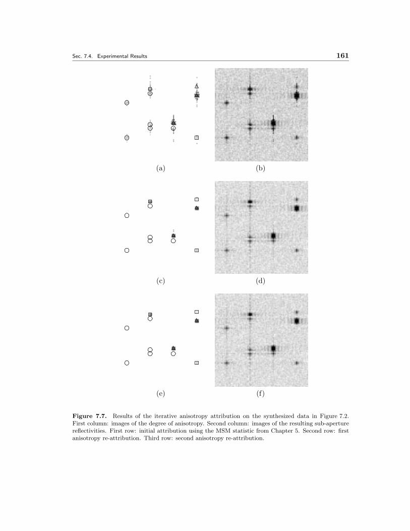
Sec. 7.4. Experimental Results 161
(a) (b)
(c) (d)
(e) (f)
Figure 7.7. Results of the iterative anisotropy attribution on the synthesized data in Figure 7.2.First column: images of the degree of anisotropy. Second column: images of the resulting sub-aperturereflectivities. First row: initial attribution using the MSM statistic from Chapter 5. Second row: firstanisotropy re-attribution. Third row: second anisotropy re-attribution.
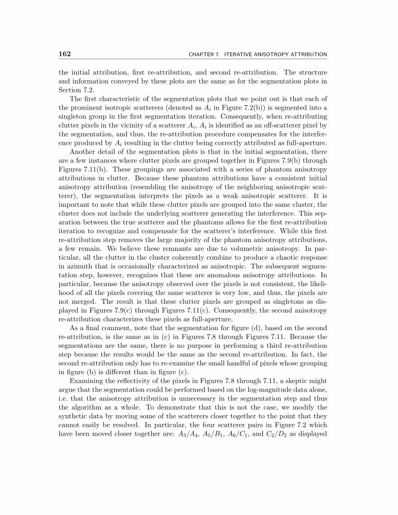
162 CHAPTER 7. ITERATIVE ANISOTROPY ATTRIBUTION
the initial attribution, first re-attribution, and second re-attribution. The structureand information conveyed by these plots are the same as for the segmentation plots inSection 7.2.
The first characteristic of the segmentation plots that we point out is that each ofthe prominent isotropic scatterers (denoted as Ai in Figure 7.2(b)) is segmented into asingleton group in the first segmentation iteration. Consequently, when re-attributingclutter pixels in the vicinity of a scatterer Ai, Ai is identified as an off-scatterer pixel bythe segmentation, and thus, the re-attribution procedure compensates for the interfer-ence produced by Ai resulting in the clutter being correctly attributed as full-aperture.
Another detail of the segmentation plots is that in the initial segmentation, thereare a few instances where clutter pixels are grouped together in Figures 7.9(b) throughFigures 7.11(b). These groupings are associated with a series of phantom anisotropyattributions in clutter. Because these phantom attributions have a consistent initialanisotropy attribution (resembling the anisotropy of the neighboring anisotropic scat-terer), the segmentation interprets the pixels as a weak anisotropic scatterer. It isimportant to note that while these clutter pixels are grouped into the same cluster, thecluster does not include the underlying scatterer generating the interference. This sep-aration between the true scatterer and the phantoms allows for the first re-attributioniteration to recognize and compensate for the scatterer’s interference. While this firstre-attribution step removes the large majority of the phantom anisotropy attributions,a few remain. We believe these remnants are due to volumetric anisotropy. In par-ticular, all the clutter in the cluster coherently combine to produce a chaotic responsein azimuth that is occasionally characterized as anisotropic. The subsequent segmen-tation step, however, recognizes that these are anomalous anisotropy attributions. Inparticular, because the anisotropy observed over the pixels is not consistent, the likeli-hood of all the pixels covering the same scatterer is very low, and thus, the pixels arenot merged. The result is that these clutter pixels are grouped as singletons as dis-played in Figures 7.9(c) through Figures 7.11(c). Consequently, the second anisotropyre-attribution characterizes these pixels as full-aperture.
As a final comment, note that the segmentation for figure (d), based on the secondre-attribution, is the same as in (c) in Figures 7.8 through Figures 7.11. Because thesegmentations are the same, there is no purpose in performing a third re-attributionstep because the results would be the same as the second re-attribution. In fact, thesecond re-attribution only has to re-examine the small handful of pixels whose groupingin figure (b) is different than in figure (c).
Examining the reflectivity of the pixels in Figures 7.8 through 7.11, a skeptic mightargue that the segmentation could be performed based on the log-magnitude data alone,i.e. that the anisotropy attribution is unnecessary in the segmentation step and thusthe algorithm as a whole. To demonstrate that this is not the case, we modify thesynthetic data by moving some of the scatterers closer together to the point that theycannot easily be resolved. In particular, the four scatterer pairs in Figure 7.2 whichhave been moved closer together are: A3/A4, A5/B1, A6/C1, and C2/D2 as displayed
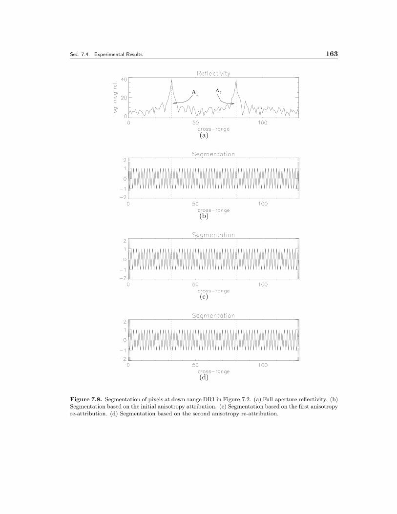
Sec. 7.4. Experimental Results 163
A1A2
(a)
(b)
(c)
(d)
Figure 7.8. Segmentation of pixels at down-range DR1 in Figure 7.2. (a) Full-aperture reflectivity. (b)Segmentation based on the initial anisotropy attribution. (c) Segmentation based on the first anisotropyre-attribution. (d) Segmentation based on the second anisotropy re-attribution.
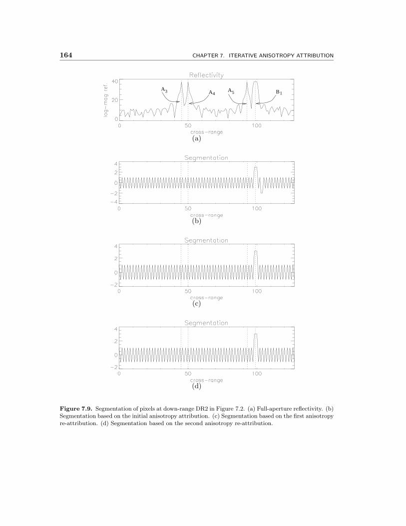
164 CHAPTER 7. ITERATIVE ANISOTROPY ATTRIBUTION
A3 A4A5 B1
(a)
(b)
(c)
(d)
Figure 7.9. Segmentation of pixels at down-range DR2 in Figure 7.2. (a) Full-aperture reflectivity. (b)Segmentation based on the initial anisotropy attribution. (c) Segmentation based on the first anisotropyre-attribution. (d) Segmentation based on the second anisotropy re-attribution.
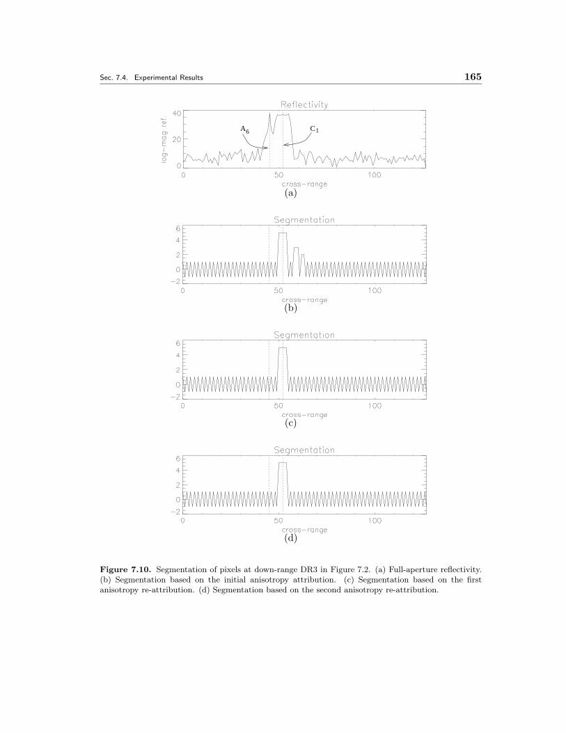
Sec. 7.4. Experimental Results 165
6 C1A
(a)
(b)
(c)
(d)
Figure 7.10. Segmentation of pixels at down-range DR3 in Figure 7.2. (a) Full-aperture reflectivity.(b) Segmentation based on the initial anisotropy attribution. (c) Segmentation based on the firstanisotropy re-attribution. (d) Segmentation based on the second anisotropy re-attribution.
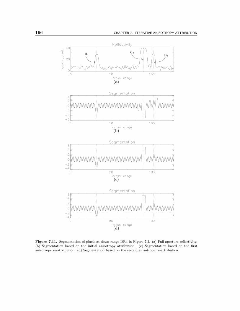
166 CHAPTER 7. ITERATIVE ANISOTROPY ATTRIBUTION
D1C2
D2
(a)
(b)
(c)
(d)
Figure 7.11. Segmentation of pixels at down-range DR4 in Figure 7.2. (a) Full-aperture reflectivity.(b) Segmentation based on the initial anisotropy attribution. (c) Segmentation based on the firstanisotropy re-attribution. (d) Segmentation based on the second anisotropy re-attribution.
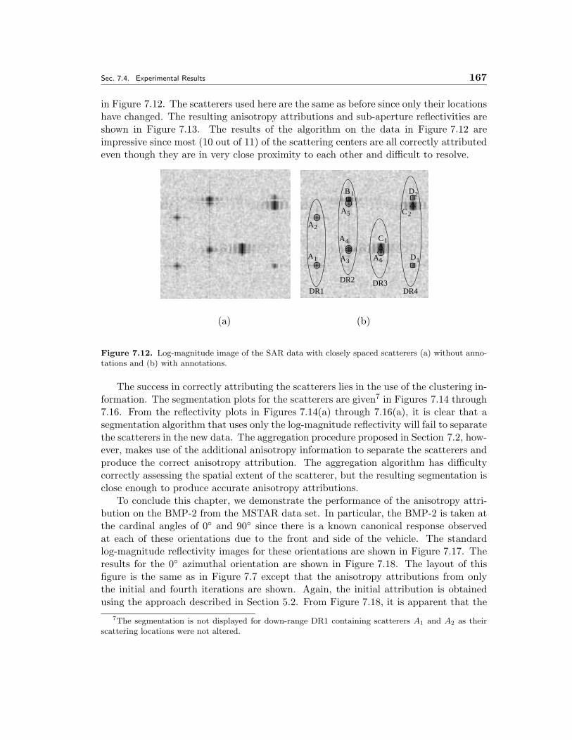
Sec. 7.4. Experimental Results 167
in Figure 7.12. The scatterers used here are the same as before since only their locationshave changed. The resulting anisotropy attributions and sub-aperture reflectivities areshown in Figure 7.13. The results of the algorithm on the data in Figure 7.12 areimpressive since most (10 out of 11) of the scattering centers are all correctly attributedeven though they are in very close proximity to each other and difficult to resolve.
1
D1
A2
A
B
A3
A
1
A4
A
5
C1
D2
C2
6
DR1
DR2 DR3DR4
(a) (b)
Figure 7.12. Log-magnitude image of the SAR data with closely spaced scatterers (a) without anno-tations and (b) with annotations.
The success in correctly attributing the scatterers lies in the use of the clustering in-formation. The segmentation plots for the scatterers are given7 in Figures 7.14 through7.16. From the reflectivity plots in Figures 7.14(a) through 7.16(a), it is clear that asegmentation algorithm that uses only the log-magnitude reflectivity will fail to separatethe scatterers in the new data. The aggregation procedure proposed in Section 7.2, how-ever, makes use of the additional anisotropy information to separate the scatterers andproduce the correct anisotropy attribution. The aggregation algorithm has difficultycorrectly assessing the spatial extent of the scatterer, but the resulting segmentation isclose enough to produce accurate anisotropy attributions.
To conclude this chapter, we demonstrate the performance of the anisotropy attri-bution on the BMP-2 from the MSTAR data set. In particular, the BMP-2 is taken atthe cardinal angles of 0◦ and 90◦ since there is a known canonical response observedat each of these orientations due to the front and side of the vehicle. The standardlog-magnitude reflectivity images for these orientations are shown in Figure 7.17. Theresults for the 0◦ azimuthal orientation are shown in Figure 7.18. The layout of thisfigure is the same as in Figure 7.7 except that the anisotropy attributions from onlythe initial and fourth iterations are shown. Again, the initial attribution is obtainedusing the approach described in Section 5.2. From Figure 7.18, it is apparent that the
7The segmentation is not displayed for down-range DR1 containing scatterers A1 and A2 as theirscattering locations were not altered.
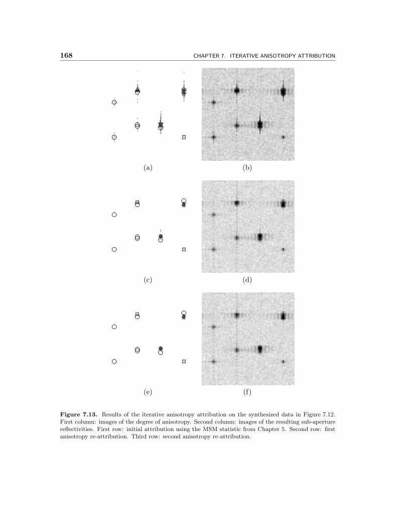
168 CHAPTER 7. ITERATIVE ANISOTROPY ATTRIBUTION
(a) (b)
(c) (d)
(e) (f)
Figure 7.13. Results of the iterative anisotropy attribution on the synthesized data in Figure 7.12.First column: images of the degree of anisotropy. Second column: images of the resulting sub-aperturereflectivities. First row: initial attribution using the MSM statistic from Chapter 5. Second row: firstanisotropy re-attribution. Third row: second anisotropy re-attribution.
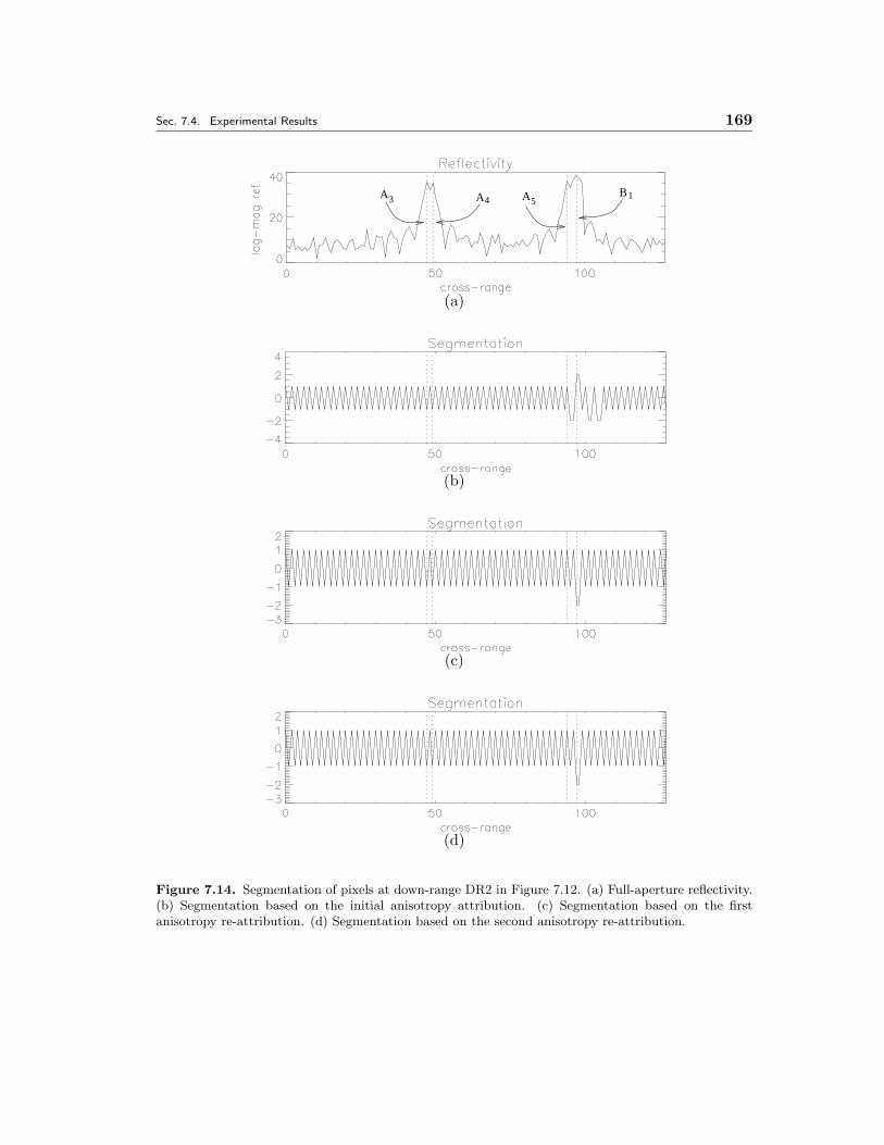
Sec. 7.4. Experimental Results 169
5A4A3B1A
(a)
(b)
(c)
(d)
Figure 7.14. Segmentation of pixels at down-range DR2 in Figure 7.12. (a) Full-aperture reflectivity.(b) Segmentation based on the initial anisotropy attribution. (c) Segmentation based on the firstanisotropy re-attribution. (d) Segmentation based on the second anisotropy re-attribution.
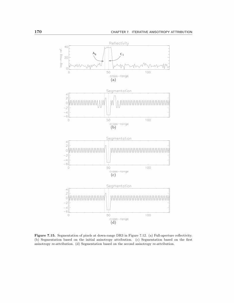
170 CHAPTER 7. ITERATIVE ANISOTROPY ATTRIBUTION
6 C1A
(a)
(b)
(c)
(d)
Figure 7.15. Segmentation of pixels at down-range DR3 in Figure 7.12. (a) Full-aperture reflectivity.(b) Segmentation based on the initial anisotropy attribution. (c) Segmentation based on the firstanisotropy re-attribution. (d) Segmentation based on the second anisotropy re-attribution.
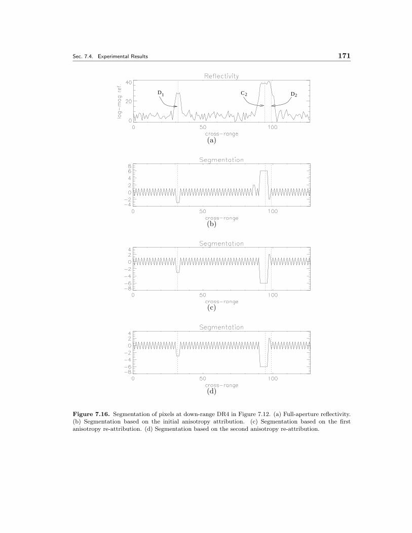
Sec. 7.4. Experimental Results 171
2C2 DD1
(a)
(b)
(c)
(d)
Figure 7.16. Segmentation of pixels at down-range DR4 in Figure 7.12. (a) Full-aperture reflectivity.(b) Segmentation based on the initial anisotropy attribution. (c) Segmentation based on the firstanisotropy re-attribution. (d) Segmentation based on the second anisotropy re-attribution.
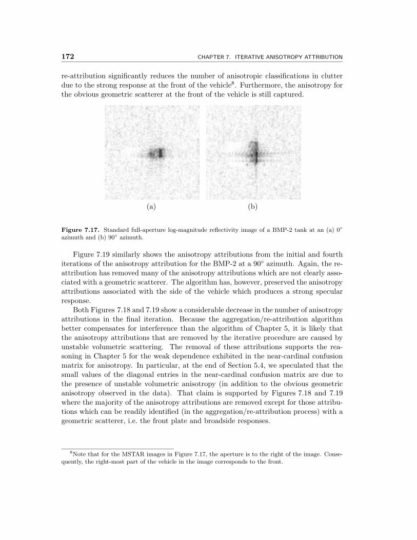
172 CHAPTER 7. ITERATIVE ANISOTROPY ATTRIBUTION
re-attribution significantly reduces the number of anisotropic classifications in clutterdue to the strong response at the front of the vehicle8. Furthermore, the anisotropy forthe obvious geometric scatterer at the front of the vehicle is still captured.
(a) (b)
Figure 7.17. Standard full-aperture log-magnitude reflectivity image of a BMP-2 tank at an (a) 0◦
azimuth and (b) 90◦ azimuth.
Figure 7.19 similarly shows the anisotropy attributions from the initial and fourthiterations of the anisotropy attribution for the BMP-2 at a 90◦ azimuth. Again, the re-attribution has removed many of the anisotropy attributions which are not clearly asso-ciated with a geometric scatterer. The algorithm has, however, preserved the anisotropyattributions associated with the side of the vehicle which produces a strong specularresponse.
Both Figures 7.18 and 7.19 show a considerable decrease in the number of anisotropyattributions in the final iteration. Because the aggregation/re-attribution algorithmbetter compensates for interference than the algorithm of Chapter 5, it is likely thatthe anisotropy attributions that are removed by the iterative procedure are caused byunstable volumetric scattering. The removal of these attributions supports the rea-soning in Chapter 5 for the weak dependence exhibited in the near-cardinal confusionmatrix for anisotropy. In particular, at the end of Section 5.4, we speculated that thesmall values of the diagonal entries in the near-cardinal confusion matrix are due tothe presence of unstable volumetric anisotropy (in addition to the obvious geometricanisotropy observed in the data). That claim is supported by Figures 7.18 and 7.19where the majority of the anisotropy attributions are removed except for those attribu-tions which can be readily identified (in the aggregation/re-attribution process) with ageometric scatterer, i.e. the front plate and broadside responses.
8Note that for the MSTAR images in Figure 7.17, the aperture is to the right of the image. Conse-quently, the right-most part of the vehicle in the image corresponds to the front.
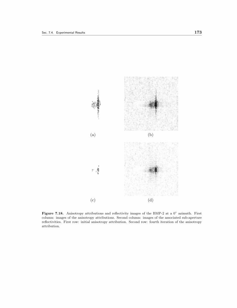
Sec. 7.4. Experimental Results 173
(a) (b)
(c) (d)
Figure 7.18. Anisotropy attributions and reflectivity images of the BMP-2 at a 0◦ azimuth. Firstcolumn: images of the anisotropy attributions. Second column: images of the associated sub-aperturereflectivities. First row: initial anisotropy attribution. Second row: fourth iteration of the anisotropyattribution.
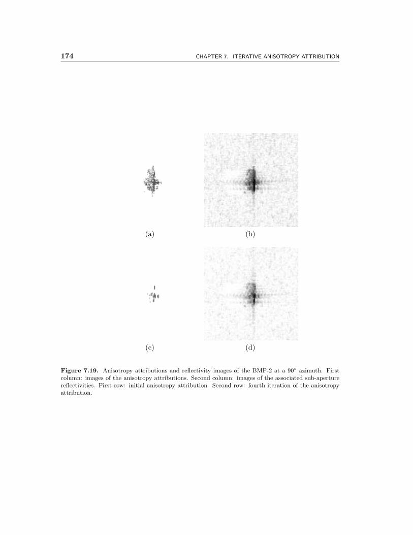
174 CHAPTER 7. ITERATIVE ANISOTROPY ATTRIBUTION
(a) (b)
(c) (d)
Figure 7.19. Anisotropy attributions and reflectivity images of the BMP-2 at a 90◦ azimuth. Firstcolumn: images of the anisotropy attributions. Second column: images of the associated sub-aperturereflectivities. First row: initial anisotropy attribution. Second row: fourth iteration of the anisotropyattribution.
Chapter 8
Contributions andSuggestions for Future Research
This thesis contributes to the field of SAR ATR through the exploitation of nonidealscatterer anisotropy. Two fundamental methodologies are used towards this end. Thefirst is a nonparametric approach that classifies targets based on observed anisotropybehavior that is learned from the data. The second (and more developed) approach is aparametric characterization of the unimodal azimuthal response that is common fromcanonical scatterers. This chapter summarizes these contributions in Section 8.1 andprovides suggestions for further research in Section 8.2.
� 8.1 Summary of Contributions
This section summarizes the contributions of this thesis by chapter.
Sub-aperture Representation
The cornerstone of the analysis in this thesis is the sub-aperture pyramid presented inChapter 3. This structure divides the aperture into various sub-apertures and arrangesthem in a manner that allows for the exploitation of scatterer anisotropy throughoutthe remainder of the thesis. One function of the pyramid is to represent the data inan over-complete basis that reveals anisotropic scattering. In particular, each level ofthe pyramid corresponds to a particular cross-range–azimuthal resolution trade-off. Notonly does the pyramid provide a library of representations, but these representations arestructured such that anisotropy in the data exhibit distinctive patterns in the pyramid.In particular, unimodal azimuthal scattering appears as a “streak” down the pyramidof reflectivity estimates where properties of the streak convey information about theanisotropy.
The data in the pyramid are used in two ways. The first is a nonparametric approachin which the patterns of the data are learned with a Parzen density estimator. Thesecond approach uses the sub-apertures to define anisotropy hypotheses and uses thesub-aperture reflectivity measurements as observations to test the hypotheses. Thesub-aperture scattering hypotheses approximate the unimodal anisotropic scattering
175
176 CHAPTER 8. CONTRIBUTIONS AND SUGGESTIONS FOR FUTURE RESEARCH
predicted by physics-based models for many canonical scattering types. In particular,the hypotheses characterize the degree of anisotropy which is related to scatterer size.
Nonparametric Estimation of Anisotropy
Chapter 4 of this thesis extends the density-based classification approach presented byDeBonet et. al.[20]. In both approaches, an image is characterized by generating aset of features whose statistical relationships are learned with a nonparametric densityestimator. This learning process is applied to an image of an unknown target and imagesof reference vehicles. A classification decision is then made by comparing the densitylearned from the unknown target image to the densities learned from the referenceimages.
The work in Chapter 4 extends DeBonet’s method in two ways. The first is our useof the sub-aperture feature set which is motivated by scattering physics, in contrastto DeBonet’s wavelet-based feature set that is motivated by image texture. The sub-aperture feature vector is taken as the pyramid of log-magnitude sub-aperture reflec-tivities for a given location. These reflectivities convey the variations of the azimuthalresponse produced by a scatterer.
The other extension of DeBonet’s work is in the manner in which the divergencecomparing two densities is approximated. DeBonet uses a summation motivated by thelaw of large numbers. This approximation, however, can lead to the use of an excessivenumber of samples in the summation. In particular, DeBonet’s approximation tends toevaluate the summand at a high number of clutter samples due to the predominance ofclutter in the image. The approximation proposed in Section 4.2.4, however, is based ona Riemann sum where the samples are uniformly spread throughout the feature spacethus preventing too many samples from being allocated toward clutter. The result is asignificant reduction in the computation required.
Sub-aperture Anisotropy Attribution
Chapter 5 develops a method for attributing anisotropy. The basis of the attribution isthe sub-aperture scattering model introduce by Chaney et. al.[12] and Allen et. al.[2]that characterizes the azimuthal response from a scatterer. The attribution is obtainedby developing an LRT for anisotropy hypotheses defined from the sub-aperture pyramid.The first test presented is a GLRT in which the ML reflectivity estimate (under theassociated anisotropy hypothesis) is used for the value of the reflectivity parameter.The resulting GLLR is called the basic GLLR statistic and corresponds to a differencein average sub-aperture energy between the two sub-aperture hypotheses comprisingthe likelihood ratio. Thus, average sub-aperture energy is a sufficient statistic for thismodel.
While the basic GLLR statistic is consistent with our intuition for characterizingazimuthal concentration, it is not robust to interference from neighboring scattererswhich the sub-aperture scattering model does not include. This issue is addressed in twoways. The first address is to recognize that the ML estimate (under a given anisotropy
Sec. 8.1. Summary of Contributions 177
hypothesis) of reflectivity has a corresponding resolution that varies with the hypothesis,and thus, the hypotheses are not consistent with each other. To deal with this issue,a scaling of the measured full-aperture reflectivity is used to estimate the sub-aperturereflectivity, where the scaling factor provides the appropriate normalization for usingthe full-aperture to measure a partial-aperture response. Under this approach, all thereflectivity estimates are imaged at the finest resolution, and thus, the hypotheses areconsistent with each other. This new reflectivity estimate results in a slight modificationof the basic GLLR statistic. In particular, a term penalizing the amount of energyoutside the hypothesized sub-aperture is added to the statistic. This modified GLLRstatistic significantly improves the accuracy of the anisotropy attribution, but the effectsof interfering scatterers are still evident.
The second method used to address interfering scatterers explicitly includes theireffects in the scattering model. In particular, the sub-aperture scattering model is ex-tended to allow for scatterers at neighboring pixel locations. In this extended model,the nuisance reflectivity parameter corresponds to a vector of reflectivities. These re-flectivities are estimated in an ML fashion using a Gaussian prior on the reflectivities toregularize the estimation problem. The estimated reflectivities are then used to deter-mine a likelihood statistic for the sub-aperture hypotheses. The LRT using this MSMstatistic performs better than the modified GLLR but is still vulnerable to interferencefrom neighboring scatterers.
To address the effects of interfering scatterers beyond the use of the modified GLLRand MSM statistics, Section 5.3 proposes performing the hypothesis tests in a tele-scopic, decision-directed fashion to take advantage of the structure provided by thesub-aperture pyramid. The telescopic testing procedure starts at the top of the pyra-mid and traverses a path down the pyramid following the most likely sub-aperturehypothesis at each step. Not only does this testing reduce the number of sub-aperturesthat need to be tested, but the telescopic testing enforces a consistency between thesub-aperture hypotheses which reduces the number of anisotropic classifications due tointerfering scatterers.
The chapter concludes with application of the anisotropy attribution to the MSTARdata. To evaluate the utility provided by the anisotropy attribution, confusion matricesfor the attribution are empirically estimated. In particular, the confusion matrices areseparately presented for the case of near-cardinal and off-cardinal orientations. Thenear-cardinal orientations exhibit a mild dependence of the “test” attribution on the“truth” attribution, although this dependence is not as strong as we had expected. Theanisotropy attribution for off-cardinal orientations is even less stable in the sense thatthe “test” attribution is independent of the “truth” attribution. We conjectured thatthe source of the instability is volumetric scattering which arises from the interferenceof irresolvable scatterers and produces an erratic, scintillating response in azimuth.Thus, the anisotropy characterization of these volumetric scatterers is also erratic asthe azimuthal energy concentration fluctuates and is thus sensitive to slight changes inimaging orientation. The aperture used in the MSTAR data is too narrow to observe
178 CHAPTER 8. CONTRIBUTIONS AND SUGGESTIONS FOR FUTURE RESEARCH
anisotropy due to canonical scatterers except at near-cardinal orientations. The remain-der of the anisotropy attributions are thus believe to be due to volumetric scatterers.This limited observation of canonical scattering explains the weak dependence observedat near-cardinal azimuths and the independence observed at off-cardinal azimuths inthe MSTAR data.
Relation Between Phenomenology and Anisotropy Attribution
The results on the MSTAR data in Chapter 5 motivated the study in Chapter 6 ofanisotropy phenomenology and its effects on anisotropy attribution. Two sources ofanisotropy are considered in this chapter. The first is the class of geometric scattererswhich have a simple geometric structure and produce a consistent anisotropic response.The second source considered is the class of volumetric scatterers that are composed ofirresolvable point scatterers that interfere in a manner resulting in a chaotic azimuthalresponse which is occasionally characterized as anisotropic. For each case, the informa-tion conveyed by the anisotropy attribution is evaluated. In particular, anisotropy plotsare shown to convey the dependence of the anisotropy attribution on the scatterer “size”.For geometric scatterers, we find that there is a strong dependence of the anisotropyattribution on the scatterer size. Furthermore, the attributions are consistent with theactual concentration of the azimuthal response. However, for volumetric scatterers, wedemonstrated that the strength of the dependence varies with the underlying scattererdensity. In particular, for low-density volumetric scatterers, the anisotropy attributionis independent of scatterer size and the full-aperture attribution is usually produced.For high-density volumetric scatterers, the anisotropy attribution is highly dependenton scatterer size because the scatterer resembles a geometric scatterer.
It is argued and demonstrated in this chapter that by using a wider aperture, one canreduce the incidence of observed volumetric anisotropy while preserving the observedgeometric anisotropy which is more meaningful in characterizing the scatterer. The task,however, is not as simple as just increasing aperture length. In particular, the effectsof location uncertainty must be addressed. Increasing the aperture length increases thelocation uncertainty for physically large geometric scatterers, but reduces the locationuncertainty for volumetric scatterers. To address this apparent conflict, we presented adecision-directed peak extraction method that uses the anisotropy attribution to adaptthe resolution of the peak extraction to the underlying scatterer.
Chapter 6 also demonstrates the benefit of additional anisotropy hypotheses thatwide-aperture data allows to be defined. Larger sub-apertures can be used to form sub-aperture hypotheses which better characterize the anisotropy produced by smaller scat-terers. In narrow-aperture settings, these small scatterers may produce an azimuthalresponse whose mainlobe is wider than the aperture and thus can only be characterizedas full-narrow-aperture. However, with a larger aperture, the localized concentrationof this response in azimuth can be better characterized as the full-narrow-apertureattribution is no longer the minimal anisotropy characterization available.
Sec. 8.2. Suggestions for Future Research 179
Iterative Anisotropy Attribution
Chapter 7 returns to the task of improving the anisotropy attribution. An iterativeapproach is proposed to model and remove the effects of interfering scatterers. Theproposed iteration is a two step procedure that first clusters pixels according to theircorresponding scatterers and then re-attributes pixels using the clustering informationto suppress the effects of neighboring scatterers. The clustering is performed with agreedy algorithm that maximizes the likelihood of an observed set of features corre-sponding to pixel reflectivity, pixel anisotropy, and scatterer size. Due to the mannerin which the observed features are modeled, an additive cost function can be used toevaluate the likelihood of a segmentation. Evaluation of all possible segmentations iscomputationally prohibitive. Thus, the ML segmentation is approximated by a greedyalgorithm that at each iteration merges the two regions which result in the largestincrease of the likelihood.
The re-attribution procedure extends the regularization approach of Section 5.2. Inparticular, the vector of reflectivities (of the focused pixel and its neighbors) is modeledas a noisy observation of the finest resolution reflectivity measurements instead of a zero-mean Gaussian prior (as done in Chapter 5). Incorporating this observation model intothe estimation of the reflectivity nuisance parameter produces a term that regularizesthe estimate towards the observed reflectivities. In addition, as described in Chapter 7,the aggregation of pixels into distinct, physically extended scatterers allows us to devisean improved method for removing interference from such neighboring scatterers.
The results from using the iterative clustering–re-attribution procedure are quiteaccurate. Significant improvements are made over the attribution of Chapter 5. Inparticular, virtually all of the anisotropy misclassifications (due to interference from aneighboring scatterer) in clutter are removed. Furthermore, the attribution of weakscatterers that are corrupted by neighboring strong scatterers are also improved.
� 8.2 Suggestions for Future Research
The research presented in this thesis opens several new directions for further researchwhich are described in this section.
Sub-band Analysis
The focus of this thesis has been on sub-aperture analysis to exploit aspect dependentscattering in azimuth. This work is motivated by the physics-based PO and GTD scat-tering models which predict aspect dependencies based upon the canonical scatterertype, e.g. flat plate, dihedral, trihedral, top-hat, sphere, etc.. The PO and GTD scat-tering models also predict a similar dependence in frequency. Frequency is analogousto azimuth but for the down-range component instead of cross-range. The PO andGTD models predict that frequency concentration characterizes down-range extent inthe same way that azimuthal concentration characterizes cross-range extent. The POresponse for several canonical scatterers is presented in Eqs. (2.16)-(2.19) of Chapter 2.
180 CHAPTER 8. CONTRIBUTIONS AND SUGGESTIONS FOR FUTURE RESEARCH
Because of the similarity between frequency and azimuth, much of the sub-apertureanalysis should carry over sub-band analysis. However, there are two differences thatone should keep in mind when adapting the sub-aperture analysis to frequency. Onedifference is that the sinc-like dependence is actually a function of the reciprocal offrequency instead of frequency. Thus, the mode of the sinc will occur at the highestfrequency in the band. However, besides this sinc component of the response there isan additional scaling factor of the form fn/2 where n is an integer (positive, negative, orzero) that is determined by the canonical scatterer type. Negative values of n may shiftthe location of the mode to something other than the highest frequency. Furthermore,this frequency dependent scaling factor may significantly modify the envelope on theresponse, especially in ultra-wideband data. It is suspected that because the methodsin Chapters 5 and 7 have been developed to be robust to slight functional deviationsin the modeled response, this additional factor in the frequency dependence shouldnot significantly detract from the applicability of the analysis to frequency instead ofazimuth. However, such supposition should be studied and verified, and not taken asfact.
The application of the sub-aperture analysis to frequency is not expected to posesignificant new challenges; however, this expectation assumes that one does sub-bandanalysis instead of sub-aperture analysis. If one wishes to do both sub-band andsub-aperture analysis simultaneously, the problem becomes considerably more difficult.Problems manifest themselves at the very core of the analysis with the generalizationof the sub-aperture pyramid. An intuitive generalization is to extend the pyramid toa two dimensional structure resembling the quad-trees used in the multiscale analysisof images. In such an extension, the intervals corresponding to sub-apertures now gen-eralize into “squares” that are the product of a sub-aperture and sub-band. Such ageneralization seriously restricts the scattering phenomena that can accurately be cap-tured in a concise manner. In particular, there is no reason to believe that just becausescattering energy is concentrated in azimuth (or frequency) that the energy is concen-trated in frequency (or azimuth). For example, a scatterer whose down-range extent issignificantly smaller than its cross-range extent will have a broad energy distributionin frequency, but a high energy concentration in azimuth. Such a scatterer would notbe concisely captured in the proposed pyramidal representation. With such scatterersin mind, we believe that one would have to generalize the pyramid to
S × S = {Sm,i × Sn,j
∣∣Sm,i, Sn,j ∈ S}
in order to capture scatterers whose cross-range and down-range extents do not match.Besides extending the pyramidal representation, there is also the issue of how to
model neighboring scatterers which are now located in both down-range and cross-range.To model all neighboring pixels, as done in this thesis, is computationally burdensomedue to significant increase in the model order from N (neighboring pixels in cross-rangeat a single range) to N2 (neighboring pixels in both cross-range and down-range).Considering that the iterative approach in Chapter 7 involves a matrix inversion, the
Sec. 8.2. Suggestions for Future Research 181
high cost of using all N2 neighboring pixels is clear. Practical application of such modelswill almost certainly need to exploit the sparsity of scatterers in the imagery.
Replacing the Sub-aperture Scattering Model
The sub-aperture scattering model is used to model anisotropy both because of itssimplicity and its general characterization of azimuthal concentration. An interestingdirection for further research is to evaluate the efficacy of other models for the azimuthalresponse. A drawback of the sub-aperture scattering model is that the correspondingresponse in the image domain is a sinc function. Because the sinc function has aninfinite extent, it is clear that no scatterer will truly fit this response. Furthermore, theslow spatial decay of this response may leave the attribution unnecessarily vulnerable tostrong interfering scatterers. With this thought in mind, it may seem obvious that someother function, which decays faster in the spatial domain, should be used. Examples ofalternative azimuthal response model are the sinc function (corresponding to a boxcarin the spatial domain) and the Gaussian pulse (corresponding to a Gaussian pulse in thespatial domain). One must be cautious, however, in using other azimuthal scatteringmodels. In particular, there is the issue of how modeling errors in the azimuthal domainwill effect the resulting anisotropy test. As an example, consider using a boxcar in thespatial domain (or equivalently a sinc in the azimuthal domain). The sensitivity of theanisotropy test to the misalignment of the zero crossings of the modeled sinc to theactual response1 needs to be taken into consideration. This misalignment may be dueto either a difference in the fundamental frequency of the two responses or a differencein the azimuthal location of the mainlobe. Regardless of the source, if the misalignmentis severe enough, then there may be sub-apertures in which the sidelobes of the modeledand actual azimuthal response are 180◦ out of phase resulting in a significant error inthat sub-aperture.
We believe that gains can be achieved by using a better model than the sub-aperturescattering model. Our intuition is that a sinc azimuthal response (or any other az-imuthal response with significant oscillations) will not be significantly more effectivethan the boxcar response due to problems with the alignment of the zero-crossings.However, we suspect that smooth unimodal functions, such as the Gaussian, wouldperform better than the sub-aperture scattering model. Because such a function doesnot change sign, there is no concern about the alignment of zero-crossings. Further-more, because the model function is smooth, it will exhibit faster decay in the imagedomain than the sub-aperture scattering model.
Measure of Sub-aperture Stability
In Chapter 6, we discuss how the use of a wider aperture can reduce the incidence ofvolumetric anisotropy. This reduction can be achieved because volumetric scatterersproduce a chaotic azimuthal response whose energy is distributed across the aperture,
1Many scatterers produce an azimuthal response which oscillates.
182 CHAPTER 8. CONTRIBUTIONS AND SUGGESTIONS FOR FUTURE RESEARCH
while geometric scatterers produce a highly concentrated azimuthal response. However,this approach does not provide perfect rejection of volumetric scatterers. An interest-ing direction for further research is to characterize each anisotropy attribution with aconfidence measure conveying how likely it corresponds to geometric anisotropy ratherthan volumetric anisotropy. Such a confidence measure could be used in tandem withthe anisotropy attribution to weight its importance in a classification algorithm.
The intuitive motivation for obtaining this measure is the same as the intuitionbehind the reduction of volumetric anisotropy in wide-aperture data. In particular,we believe that a measure that characterizes the goodness-of-fit of the observed az-imuthal response to the hypothesized azimuthal response should convey how likely ananisotropy attribution is due to a geometric scatterer rather than a volumetric scat-terer. Because volumetric scatterers produce a chaotic azimuthal response, even if theresponse is declared anisotropic, the hypothesized azimuthal response will be a poor fitto the volumetric scatterer’s actual response. A geometric scatterer on the other handshould demonstrate a very high similarity to the modeled azimuthal response due to itsstructured, highly concentrated azimuthal response.
This idea is similar in spirit to the work of Smith et. al.[51] where they propose anad-hoc “peak-stability” measure to characterize the deviation of the azimuthal responsefrom the isotropic response. We believe that a principled statistic can be obtained whichalso applies to sub-aperture scattering models.
Extending the Hybrid-Resolution Peak Extraction
The hybrid-resolution peak extraction/attribution used in Chapter 6 uses a decision-directed method to determine which resolution should be used for the anisotropy at-tribution. The method first examines the anisotropy attribution for the fine-resolutionpeak extraction, and if the attribution is anisotropic, then the coarse-resolution peakextraction is used for the attribution. This approach was restricted to the use of tworesolutions for simplicity and to demonstrate proof-of-concept for the suppression ofvolumetric anisotropy in wide-aperture data. The approach should be generalized touse more than just two pre-determined resolutions for the peak extraction. We believeit would be more effective (both for the peak extraction and the anisotropy attribution)to perform the peak extraction and anisotropy attribution in alternating steps. In par-ticular, the peak extraction is repeatedly performed at successively coarser resolutionsuntil the anisotropy attribution produced for the peak extraction conveys a scatterersize that is consistent with the resolution at which the peak of the scatterer is extracted.
Appendix A
DeBonet’s Wavelet-based Classifier
In [20], DeBonet et. al. introduce a SAR classifier that exploits the differences in cross-scale dependencies in image data to distinguish various targets. The classification set-ting and underlying principles of the algorithm proposed by DeBonet are the same asthose described in Section 2.4. In this appendix, DeBonet’s approach is described inmore detail using the notation and ideas from Section 2.4. The cross-scale dependen-cies are learned in a nonparametric fashion by applying the Parzen density estima-tor to feature vectors constructed from a multiresolution representation of the imagedata. Classification decisions are then made by comparing the density estimate froman unknown target to density estimates from labeled targets as in Section 2.4.3. Theremainder of this appendix describes these steps in more detail. Section A.1 presentsthe wavelet-based feature set used to represent the data. Section A.2 describes howthese features are learned. Section A.3 then discusses how the estimated densities areused to classify vehicles.
� A.1 Wavelet-based Representation
DeBonet bases his data representation on the wavelet transform1 which represents theimage data at multiple resolutions. The SAR data used in DeBonet’s approach is thelog-magnitude SAR image, i.e. the phase information is discarded. Starting from thisimage, DeBonet generates a sequence of multiresolution images by recursively applyingthe wavelet transform and down-sampling by a factor of two to obtain the low-frequencycomponent of the image as illustrated in the left-hand side of Figure A.1. In this figure,W represents a circular convolution with the scaling function for the wavelet, ↓ 2 repre-sents a down-sampling by two in each image dimension, and Gm represents the imageat scale m with m = 0 denoting the finest resolution and m = M denoting the coarsestresolution. These images correspond to a sequence of nested sub-space representationsat successive resolutions. DeBonet applies a series of filters fm,1, fm,2, . . . , fm,N to Gm
to reveal particular structures at that scale as illustrated in the right side of Figure A.1.In particular, DeBonet uses oriented Laplacian filters for the filters fm,i. The imageresulting from the application of filter fm,i to image Gm is denoted as Fm,i.
1It is assumed that the reader is familiar with wavelets. For a thorough treatment of wavelets, thereader is referred to Cohen[14], Vetterli[57], Wickerhauser[59], and Daubechies[18].
183
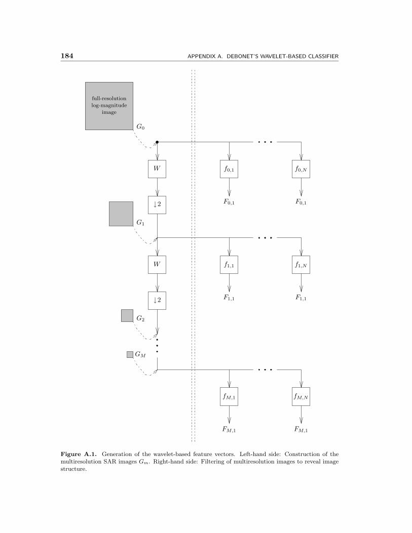
184 APPENDIX A. DEBONET’S WAVELET-BASED CLASSIFIER
f1,1 f1,N
F1,1 F1,1
f0,1 f0,N
F0,1 F0,1
fM,1 fM,N
FM,1 FM,1
W
↓2
W
↓2
full-resolution
log-magnitude
image
G0
G1
G2
GM
Figure A.1. Generation of the wavelet-based feature vectors. Left-hand side: Construction of themultiresolution SAR images Gm. Right-hand side: Filtering of multiresolution images to reveal imagestructure.
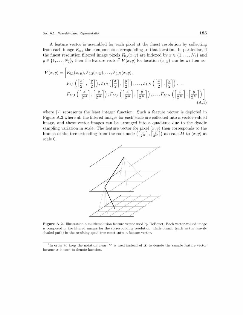
Sec. A.1. Wavelet-based Representation 185
A feature vector is assembled for each pixel at the finest resolution by collectingfrom each image Fm,i the components corresponding to that location. In particular, ifthe finest resolution filtered image pixels F0,i(x, y) are indexed by x ∈ {1, . . . , N1} andy ∈ {1, . . . , N2}, then the feature vector2 V (x, y) for location (x, y) can be written as
V (x, y) =[F0,1(x, y), F0,2(x, y), . . . , F0,N (x, y),
F1,1
(⌈x2
⌉,⌈y2
⌉), F1,2
(⌈x2
⌉,⌈y2
⌉), . . . , F1,N
(⌈x2
⌉,⌈y2
⌉), . . .
FM,1
(⌈ x
2M⌉,⌈ y
2M⌉)
, FM,2
(⌈ x
2M⌉,⌈ y
2M⌉)
, . . . , FM,N
(⌈ x
2M⌉,⌈ y
2M⌉) ](A.1)
where $·% represents the least integer function. Such a feature vector is depicted inFigure A.2 where all the filtered images for each scale are collected into a vector-valuedimage, and these vector images can be arranged into a quad-tree due to the dyadicsampling variation in scale. The feature vector for pixel (x, y) then corresponds to thebranch of the tree extending from the root node
(⌈x2M
⌉,⌈ y2M
⌉)at scale M to (x, y) at
scale 0.
Figure A.2. Illustration a multiresolution feature vector used by DeBonet. Each vector-valued imageis composed of the filtered images for the corresponding resolution. Each branch (such as the heavilyshaded path) in the resulting quad-tree constitutes a feature vector.
2In order to keep the notation clear, V is used instead of X to denote the sample feature vectorbecause x is used to denote location.
186 APPENDIX A. DEBONET’S WAVELET-BASED CLASSIFIER
� A.2 Learning Dependencies
DeBonet uses the wavelet-based feature set to reveal the cross-scale dependencies in aSAR image. To characterize these dependencies, he uses the Parzen density estimatorin Eq. (2.20) with a hyper-cube kernel, i.e.
f(v) =1
N1N2hd
N1N2∑i=1
∥∥∥∥v − V i
h
∥∥∥∥∞
(A.2)
where the V i are the feature vectors generated from an image, ‖·‖∞ denotes the infinitynorm, and each side of the hyper-cube3 measures 2h.
� A.3 Decision Rule
To classify targets in images, DeBonet compares density estimates from reference data,i.e. images whose contents are known, to density estimates from test data, i.e. imageswhose contents are to be classified. The measure for this comparison is the Chi-Squaredivergence which is a second-order approximation to twice the KL divergence[15],i.e. 2D(f0‖fl), and is given as
χ2(fl, f0) =∫ (
fl(V )− f0(V ))2
fl(V )dV (A.3)
for a reference density estimate fl and test density estimate f0. This χ2 divergence iscomputed between the density estimated from the test data and each of the densitiesestimated from the reference data. A classification decision is then made according tothe rule
l =
{l∗ � argminl
{χ2(fl, f0)
}: if χ2(fl∗ , f0) ≤ T
no classification : if χ2(fl∗ , f0) > T(A.4)
for a threshold T . Thus, the test data is declared to have arisen from the same sourcedistribution as the reference data set that minimizes the χ2 divergence as long as theresulting χ2 divergence does not exceed the threshold T . If the minimum χ2 divergenceexceeds this threshold, then a “no classification” decision is made. The threshold thusimposes a minimal confidence requirement in order to make a classification.
3The use of the hyper-cube is no less general than the use of a hyper-rectangle as the kernel becausethe filters fm,i can be used to scale the data.
Sec. A.3. Decision Rule 187
Exact computation of the integral in Eq. (A.3) is computationally intensive. DeBonetthus approximates the integral as
χ2(fl, f0) ≈∑
V ∈Sl
1
fl(V )
(fl(V )− f0(V )
)2fl(V )
=∑
V ∈Sl
(fl(V )− f0(V )
fl(V )
)2
. (A.5)
In this approximation, DeBonet replaces the integral with a summation evaluated atthe sample feature vectors in the reference data set Sl. In order to account for theirnonuniform distribution, the elements in the summation are weighted according to theirlocal sparsity, i.e. by the reciprocal of the density estimate. Because the points usedin the summation vary with the reference data set, the test density must be separatelyestimated for each reference data set to which it is compared.

188 APPENDIX A. DEBONET’S WAVELET-BASED CLASSIFIER
Appendix B
MSTAR Data Set
Moving and Stationary Target Acquisition and Recognition (MSTAR) is a Defense Ad-vanced Research Projects Agency (DARPA) program designed to explore and improveSAR ATR. To help achieve this goal, MSTAR released a large data set for public dis-tribution. The MSTAR data set was collected using the Sandia National LaboratorySAR sensor platform operating at an X-band frequency. In particular, the radar hada center frequency of 9.6GHz and a bandwidth of 0.59GHz which produces a one footdown-range resolution. To similarly obtain a one foot cross-range resolution, a 2.8◦
synthetic aperture was used.The MSTAR data set contains images of a variety of vehicles taken from various
orientations. In particular, compact discs are distributed with the following data:
• MSTAR Targets: This data subset contains images of the BMP-2 tank (9563,9566, c21)1, BTR-70 transport (c71), T-72 tank(132, 812, s7), and SLICY2 takenat 15◦ and 17◦ elevation angles with full aspect coverage, i.e. images formed every1◦ in azimuth3.
• MSTAR/IU Mixed Targets: This data subset contains images of the 2S1 gun(b01), BDRM-2 truck (E-71), BTR-60 transport (k10yt7532), D-7 bulldozer(92v13015), T-62 tank (A51), ZIL-131 truck (E12), ZSU-23/4 gun (d08), andSLICY taken at 15◦, 17◦, 30◦, and 45◦ elevation angles.
• MSTAR/IU T-72 Variants: This data subset contains images of the T-72 tank(A04, A05, A07, A10, A32, A62, A63, A64) under various articulations taken at15◦, 17◦, 30◦, and 45◦ elevation angles.
• MSTAR Clutter : This data subset contains images of clutter from rural and urbanareas of Huntsville, Alabama taken at a 15◦ elevation angle.
The work in this thesis only utilizes the 15◦ and 17◦ data in the “Targets” and “MixedTargets” data subsets. The 17◦ data are generally used for the learning aspects of the
1Th serial numbers of the imaged vehicles are specified in parentheses.2Sandia Labs Implementation of CYlinders (SLICY) is an artificial target composed of a few simple
canonical scatterers constructed to aid the study of scatterer phenomenology and ATR.3There are some azimuths omitted in the data set, thus there are slightly fewer than 360 images.
189
190 APPENDIX B. MSTAR DATA SET
classification process because the dense uniform sampling in azimuth (every 1◦) allowsfor all possible azimuthal dependencies to be observed. The 15◦ data are then used asthe test data for performance evaluation.
Bibliography
[1] “MSTAR (Public) Targets: T-72, BMP-2, BTR-70, SLICY”, see .http://www.mbvlab.wpafb.af.mil/public/MBVDATA.
[2] M. Allen and L. Hoff. Wide-angle Wideband SAR Matched Filter Image Formationfor Enhanced Detection Performance. In Proc. of the SPIE, Algorithms for SARImagery, volume 2230, pages 302–314, Apr. 1994.
[3] S. Barbarosa, L. Marsili, and G. Mungari. SAR Super-Resolution Imaging by SignalSubspace Projection Techniques. AEU Int. J. Electron. Commun., 50(2):133–138,1996.
[4] G. Benitz. Adaptive High-Definition Imaging. In Proc. of the SPIE, Algorithmsfor SAR Imagery, volume 2230, pages 106–119, Apr. 1994.
[5] G. Benitz. High-Definition Vector Imaging. Lincoln Lab. Journal, 10(2):147–169,1997.
[6] G. Benitz. High-Definition Vector Imaging for Synthetic Aperture Radar. In 31stAsilomar Conference on Signals, Systems, & Computers, volume 2, pages 1204–1209, Nov. 1997.
[7] G. Benitz and D. DeLong. Extensions of High Definition Imaging. In Proc. of theSPIE, Algorithms for SAR Imagery, volume 2487, pages 165–180, Apr. 1995.
[8] B. Bhanu. Automatic Target Recognition: State of the Art Survey. IEEE Trans.AES, 22(4):364–379, July 1986.
[9] B. Bhanu, D. E. Dudgeon, E. G. Zelnio, A. Rosenfeld, D. Casasent, and I. S. Reed.Guest Editorial Introduction to the Special Issue on Automatic Target Detectionand Recognition. IEEE Trans. IP, 6(1):1–6, January 1997.
[10] M. L. Bryant and F. D. Garber. SVM Classifier Applied to the MSTAR PublicData Set. In Algorithms for Synthetic Aperture Radar Imagery VI, volume 3721of Proceedings of SPIE, pages 355–360, Orlando, FL, April 1999.
191
192 BIBLIOGRAPHY
[11] J. Capon. High-Resolution Frequency-Wavenumber Spectrum Analysis. In Proc.IEEE, volume 57(8), pages 1408–1418, Aug. 1969.
[12] R. Chaney, A. Willsky, and L. Novak. Coherent Aspect-Dependent SAR ImageFormation. In Proc. of the SPIE, Algorithms for SAR Imagery, volume 2230,pages 256–274, Apr. 1994.
[13] H. Chiang and R. Moses. ATR Performance Prediction Using Attributed ScatteringFeatures. In Proc. of the SPIE, Algorithms for SAR Imagery, volume 3721, pages785–796, Apr. 1999.
[14] A. Cohen and J. Kovacevic. Wavelets: The Mathematical Background. Proceedingsof the IEEE, 84(4):514–522, Apr. 1996.
[15] T. Cover and J. Thomas. Elements of Information Theory. John Wiley and Sons,Inc., New York, 1991.
[16] H. Cox and R. Zeskin. Reduced Variance Distortionless Response (RVDR) Perfor-mance with Signal Mismatch. In 25st Asilomar Conference on Signals, Systems,& Computers, volume 2, pages 825–829, 1992.
[17] J. Curlander and R. McDonough. Synthetic Aperture Radar. John Wiley and Sons,Inc., New York, 1991.
[18] I. Daubechies. Ten Lectures on Wavelets, 1992. SIAM Press.
[19] J. DeBonet. Multiresolution Sampling Procedure for Analysis and Synthesis ofTexture Images. In ACM SIGGRAPH, 1997. in Computer Graphics.
[20] J. DeBonet, P. Viola, and J. Fisher. Flexible Histograms: A Multiresolution TargetDiscrimination Model. In Proc. of the SPIE, Algorithms for SAR Imagery, Apr.1998.
[21] S. DeGraaf. SAR Imaging via Modern 2-D Spectral Estimation Methods. IEEETrans. on Image Proc., 7(5):729–761, May 1998.
[22] R. Duda and P. Hart. Pattern Classification and Scene Analysis. John Wiley andSons, 1973.
[23] D. E. Dudgeon and R. T. Lacoss. An Overview of Automatic Target Recognition.Lincoln Laboratory Journal, 6(1):3–10, Spring 1993.
[24] C. Fosgate, H. Krim, W. Irving, W. Karl, and A. Willsky. Multiscale Segmentationand Anomaly Enhancement of SAR Imagery. IEEE Trans. on Image Proc., 6(1):7–20, Jan. 1997.
BIBLIOGRAPHY 193
[25] N. S. Friedland. Feature Characterization in the Context of Model-Based Search. InAlgorithms for Synthetic Aperture Radar Imagery III, volume 2757 of Proceedingsof SPIE, pages 253–270, Orlando, FL, April 1996.
[26] K. Fukunaga. Introduction to Statistical Pattern Recognition. Academic Press,Inc., Boston, 1990.
[27] A. Gersho and R. Gray. Vector Quantization and Signal Compression. KluwerAcademic Publishers, 1992.
[28] W. Hardle. Applied Nonparametric Regression. Cambridge University Press, Cam-bridge [England], 1989.
[29] W. Irving, P. Fieguth, and A. Willsky. An Overlapping Tree Approach to Multi-scale Stochastic Modeling and Estimation. IEEE Transactions on Image Process-ing, 6(11), November 1997.
[30] W. Irving, L. Novak, and A. Willsky. A Multiresolution Approach to Discriminat-ing Targets from Clutter in SAR Imagery. IEEE Transactions on Aerospace andElectronic Systems, 33(4):1157–1169, October 1997.
[31] W. W. Irving. Multiresolution Approach to Discriminating Targets From ClutterSAR data acquiredin SAR Imagery. In SPIE Symposium, Apr. 1995.
[32] H. Joe. Estimation of Entropy and Other Functionals of a Multivariate Density.Ann. Inst. Statist. Math, 41(4):683–697, 1989.
[33] J. B. Keller. Geometrical Theory of Diffraction. Journal of the Optical Society ofAmerica, 52:116–130, Feb. 1962.
[34] E. R. Keydel and S. W. Lee. Signature Prediction for Model-Based Automatic Tar-get Recognition. In Algorithms for Synthetic Aperture Radar Imagery III, volume2757 of Proceedings of SPIE, pages 306–317, Orlando, FL, April 1996.
[35] A. Kim, S. Dogan, J. Fisher, R. Moses, and A. Willsky. Attributing ScattererAnisotropy for Model Based ATR. In Proc. of the SPIE, Algorithms for SARImagery, volume 4053, Apr. 2000.
[36] A. Kim, J. Fisher, A. Willsky, and P. Viola. Nonparametric Estimation of AspectDependence for ATR. In Proc. of the SPIE, Algorithms for SAR Imagery, volume3721, pages 332–342, Apr. 1999.
[37] H. Krim and M. Viberg. Two Decades of Array Signal Processing Research. IEEESignal Processing Magazine, pages 67–92, July 1996.
[38] G. Leung and J. H. Shapiro. Toward a Fundamental Understanding of Multireso-lution SAR Signatures. In Algorithms for Synthetic Aperture Radar Imagery IV,volume 3070 of Proceedings of SPIE, Orlando, FL, April 1997.
194 BIBLIOGRAPHY
[39] J. Li and P. Stoica. An Adaptive Filtering Approach to Spectral Estimation andSAR Imaging. IEEE Trans. on Signal Proc., 44(6):1469–1484, June 1996.
[40] M. McClure and L. Carin. Matching Pursuits with a Wave-Based Dictionary. IEEETrans. on Sig. Proc., 45(12):2912–2927, Dec. 1997.
[41] Monzingo and Miller. Introduction to Adaptive Arrays. John Wiley and Sons, 1980.
[42] D. Munson. An Introduction To Strip-Mapping Synthetic Aperture Radar. InProc. Int. Conf. Acoust., Speech, and Signal Proc., pages 2245–2248, Apr. 1987.
[43] D. Munson and R. Visentin. A Signal Processing View of Strip-Mapping SyntheticAperture Radar. IEEE Trans. on Acoustics, Speech, and Sig. Proc., 37(12):2131–2146, Dec. 1989.
[44] G. J. Owirka, S. M. Verbout, and L. M. Novak. Template-based SAR ATR Per-formance Using Different Image Enhancement Techniques. In Algorithms for Syn-thetic Aperture Radar Imagery VI, volume 3721 of Proceedings of SPIE, pages302–319, Orlando, FL, April 1999.
[45] L. Potter and R. Moses. Attributed Scattering Centers for SAR ATR. IEEE Trans.on Image Proc., 5(1):79–91, Jan. 1997.
[46] J. A. Richards. Target Model Generation from Multiple Synthetic Aperture RadarImages. PhD thesis, Massachusetts Institute of Technology, Cambridge, MA, May2001.
[47] S. Ross. A First Course in Probability. MacMillan, New York, 1988.
[48] G. T. Ruck, D. E. Barrick, W. D. Stuart, and C. K. Krichbaum. Radar CrossSection Handbook. Plenum Press, New York, 1970.
[49] R. O. Schmidt. Multiple Emitter Location and Signal Parameter Estimation. IEEETrans. AP, 34:276–280, 1994.
[50] B. Silverman. Density Estimation for Statistics and Data Analysis. Chapman andHall, London, 1986.
[51] W. Smith, T. Irons, J. Riordan, and S. Sayre. Peak stability derived from phasehistory in synthetic aperture radar. In Proc. of the SPIE, Algorithms for SARImagery, volume 3721, pages 450–461, Apr. 1999.
[52] M. Soumekh. Fourier Array Imaging. Prentice Hall, Englewood Cliffs, NJ, 1994.
[53] N. Subotic, B. Thelen, J. Gorman, and M. Reiley. Multiresolution Detection ofCoherent Radar Targets. IEEE Trans. on Image Proc., 6(1):21–34, Jan. 1997.
[54] V. Vapnik. Statistical Learning Theory. Wiley, 1998. New York.
BIBLIOGRAPHY 195
[55] V. Vapnik. The Nature of Statistical Learning Theory. Springer, 2000. New York.
[56] V. Velten, T. Ross, J. Mossing, S. Worrell, and M. Bryant. Standard SAR ATREvaluation Experiments using the MSTAR Public Release Data Set. Technicalreport, Model Based Vision Lab, 1998.
[57] M. Vetterli and J. Kovacevic. Wavelets and Subband Coding. Prentice Hall, En-glewood Cliffs, NJ, 1995.
[58] D. Wehner. High Resolution Radar. Artech House, Norwood, MA, 1987.
[59] M. Wickerhauser. Lectures on Wavelet Packet Algorithms, Nov. 1991.
[60] J. Wissinger, R. B. Washburn, N. S. Friedland, A. Nowicki, D. R. Morgan,C. Chong, and R. Fung. Search Algorithms for Model-Based SAR ATR. In Al-gorithms for Synthetic Aperture Radar Imagery III, volume 2757 of Proceedings ofSPIE, pages 279–293, Orlando, FL, April 1996.
[61] C. P. Yeang and J. H. Shapiro. Target Detection Theory for Stripmap SAR UsingPhysics-Based Multiresolution Signatures. In Algorithms for Synthetic ApertureRadar Imagery V, volume 3370 of Proceedings of SPIE, pages 646–660, Orlando,FL, April 1998.