Exploring the effects of consumer–resource dynamics on contaminant bioaccumulation by aquatic herbivores

1582

Environmental Toxicology and Chemistry, Vol. 18, No. 7, pp. 1582–1590, 1999q 1999 SETAC

Printed in the USA0730-7268/99 $9.00 1 .00

EXPLORING THE EFFECTS OF CONSUMER–RESOURCE DYNAMICS ONCONTAMINANT BIOACCUMULATION BY AQUATIC HERBIVORES

MATTHEW SPENCER,*† NICHOLAS S. FISHER,‡ and WEN-XIONG WANG‡†Applied Biomathematics, 100 North Country Road, Setauket, New York 11733, USA

‡State University of New York at Stony Brook, Stony Brook, New York 11794-5000, USA

(Received 16 January 1998; Accepted 11 September 1998)

Abstract—We explore the consequences of consumer–resource interactions for bioaccumulation in two aquatic systems (cadmiumaccumulation in Dreissena polymorpha and polychlorinated biphenyl accumulation in calanoid copepods). We explicitly link thefeeding and growth rates of consumers to the abundance of resources under a variety of assumptions about the nature of theinteractions between them. The models are parameterized using field and laboratory data, and predictions are quantitatively comparedwith field-measured distributions of tissue concentrations. Different assumptions about consumer–resource interactions result indifferent predicted distributions of tissue concentrations and illustrate the way these interactions constrain the bioaccumulation ofcontaminants. Linking feeding and growth rates to resource abundances will be important whenever these abundances change overtime. User-friendly software will make these ideas accessible to nontheoreticians.

Keywords—Bioaccumulation Population dynamics Contaminants Simulation

INTRODUCTION

Bioaccumulation models for aquatic ecosystems [1–3] typ-ically include uptake of chemicals from both water and foodand are based on a detailed understanding of contaminant up-take and elimination in individual organisms. While the equi-librium predictions of these models often agree well with ob-served data [4], they assume constant feeding and growth rates[1,2,3], which are implausible under conditions of changingspecies abundances [5]. Consumer–resource models from pop-ulation biology provide a way to link the feeding and growthrates that influence contaminant accumulation to the abun-dances of resources [6]. In this paper, we describe examplemodels in which this link is explicitly made. Our aims are toshow that decisions about how to model the population-dy-namic component of the system have important consequencesfor bioaccumulation. Our examples are cadmium (Cd) accu-mulation in the freshwater zebra mussel Dreissena polymor-pha in Lake Erie and polychlorinated biphenyl (PCB) accu-mulation in marine calanoid copepods in the Mediterranean.For each model, we will describe and compare some of thealternative assumptions that can be made about the interactionsbetween herbivores and autotrophs and illustrate the conse-quences of these assumptions for predicted contaminant con-centrations, which we will quantitatively compare with fieldmeasurements. Finally, we will explain the significance ofthese results for predictive bioaccumulation modelling.

CADMIUM ACCUMULATION IN ZEBRA MUSSELS IN THEGREAT LAKES

Model structure and assumptions

The zebra mussel–cadmium model consists of four com-ponents: a pool of bioavailable cadmium, phytoplankton, other

* To whom correspondence may be addressed([email protected]). The current address of M. Spencer isCommunity Ecology Laboratory, Institute of Evolution, University ofHaifa, Haifa 31905, Israel.

seston (such as clay particles, bacteria, and detritus), and thezebra mussel D. polymorpha. Zebra mussels ingest both livingand nonliving particles and, although phytoplankton are prob-ably the most important component of the diet [7], other sestonmay be an important source of metals [8]. We include bothphytoplankton and other seston in the model but assume thatonly phytoplankton are energetically important [7]. We alsomodel the kinetics of cadmium uptake from the dissolvedphase by mussels as a first-order process. We predict cadmiumconcentrations in phytoplankton using an estimated biocon-centration factor (BCF). Zebra mussels have had a large impacton phytoplankton in western Lake Erie [9], but there is littleevidence that mussel abundance is closely linked to phyto-plankton density, although this seems plausible. We thereforeconsider two alternative models for the interaction betweenmussels and phytoplankton, which are a system in which mus-sel and phytoplankton biomasses affect each other and a sys-tem in which mussels affect phytoplankton biomass but phy-toplankton biomass does not affect mussel biomass. Our modelrepresents a single growing season from April to October,excluding spawning, and is parameterized using data fromwestern Lake Erie, other locations, and laboratory studies.Predictions are compared with field measurements of tissuecadmium concentration in zebra mussels from the Great Lakes.

Model equations

Our model for bioaccumulation is derived from a popula-tion-dynamic perspective [6] rather than from the more con-ventional physiological approach [1,2,3]. We assume that thetissue concentration of contaminant per unit biomass of zebramussels increases as a result of direct uptake from water andthrough assimilation of contaminated food. Tissue concentra-tions tend to decrease as a result of elimination from the bodyand increase in biomass (growth dilution). Feeding and growthrates are linear functions of phytoplankton biomass density,

Population dynamics and bioaccumulation Environ. Toxicol. Chem. 18, 1999 1583

dC5 [k 1 g(h PB 1 h SB )]E 2 (l 1 fgP)C (1)P P S Sdt

where C is cadmium concentration in mussels (mg/g); k isuptake rate constant from the dissolved phase (L/g/d); hP andhS are assimilation efficiencies of cadmium by mussels fromingested phytoplankton and other seston, respectively (dimen-sionless); g is filtration rate of water by mussels (L/g/d); P isphytoplankton biomass (g/L); S is seston concentration (g/L);BP and BS are bioconcentration factors for cadmium in phy-toplankton and seston, respectively (L/kg); E is bioavailablecadmium concentration (mg/L); l is elimination rate constantfor cadmium in mussels (per day); and f is biomass conversionefficiency of ingested phytoplankton (dimensionless). A linearrelationship between phytoplankton biomass density and feed-ing rate is appropriate because zebra mussels only reduce theirfiltration rate at extremely high particle concentrations [10].In our first case (mussel and phytoplankton biomasses affecteach other), phytoplankton growth is assumed to be limitedby nutrients and mussels and mussel biomass is affected byfeeding rate, that is,

dP P5 rP 1 2 2 gPM (2)1 2dt K

dM5 fgPM 2 mM (3)

dt

where r is phytoplankton growth rate (per day), K is phyto-plankton carrying capacity (mg/L), M is mussel biomass (g/L),and m is mussel death rate (per day). Comparing Equations 3and 1 highlights the relationship between biomass growth andcadmium dilution. fgP is the mass-specific rate of increase ofmussel biomass, resulting from food intake at a rate propor-tional to the amount of food available (Eqn. 3) and causing acorresponding dilution of cadmium concentration (Eqn. 1). Forthe second case (mussels affect phytoplankton but phytoplank-ton biomass does not influence mussel biomass), Equations 1and 2 are used to predict mussel cadmium concentration andphytoplankton dynamics, but mussel biomass is held constant.

As we are interested in dynamics over a single growingseason rather than the long-term equilibrium, we used nu-merical integration of Equations 1, 2, and 3 (or 1 and 2 wheremussel biomass was held constant) to predict cadmium con-centration in zebra mussels over time. Parameters were esti-mated from observational and experimental data as describedbelow. Wherever possible, we tried to account for uncertainty(lack of precise knowledge) in these estimates. Where only arange of values was available, we assumed a uniform distri-bution on the basis of the maximum entropy criterion [11].Where more information was available, we used distributions(e.g., triangular, lognormal) that described the observed data.Simulations were carried out using the commercial softwarepackage RAMASt Ecotoxicology (Applied Biomathematics,Setauket, NY, USA) [6,12]. Equations were solved using aRunge–Kutta algorithm with adaptive step-size variation [13].To deal with the uncertainty in parameter values, we ran 1,000replicate simulations, with each parameter sampled indepen-dently from the appropriate distribution at the start of eachreplicate. One thousand replicate simulations gives Kolmo-gorov–Smirnov 95% confidence limits of approximately 64%on output distributions [14] and should be sufficient to ensurereliable results [15]. In each case, we ran a set of 100 simu-lations with initial mussel cadmium concentration set to zeroand used the range of concentrations after 200 days (assumed

to be a uniform distribution) as the initial concentration for aset of 1,000 replicates. This had no effect on the final tissueconcentration of cadmium in zebra mussels, as a steady statewas approached by the end of the simulations, but gave a morerealistic estimate of mussel cadmium concentration early inthe season.

Parameter estimates

Bioavailable cadmium concentration. The mean concen-tration of dissolved cadmium in Lake Erie is 2.6 ng/L, with arange of 0.6 to 9.2 ng/L [16]. We approximated these datausing a lognormal distribution with mean 2.6 ng/L. Assumingthat the observed range represents the 0.1th and 99.9th per-centiles of a lognormal distribution and taking the geometricmean of the standard deviation estimates obtained from thesetwo percentiles, we estimated the standard deviation as 1.56ng/L.

Seston and phytoplankton concentrations and dynamics.Prior to zebra mussel invasion, phytoplankton in the westernbasin of Lake Erie had a summer average density of 1.66 mg/L[7], which constituted about 20% of total particles. Other ses-ton would then be 6.64 mg/L. An independent estimate of totalseston in the Hudson River is 5 mg/L [17], of which 5% isphytoplankton. This gives a concentration of 4.75 mg/L forother seston. We therefore used a uniform distribution withrange 4.75 to 6.64 mg/L to simulate other seston. The averagesummer biomass of phytoplankton in the western basin priorto zebra mussel invasion (1.66 mg/L) was used as the phy-toplankton carrying capacity, which therefore includes the ef-fects of other grazers such as zooplankton, which are not ex-plicitly modeled. Maximum phytoplankton growth rate in LakeErie is 1.3/d [18]. The initial phytoplankton biomass was setto 1.25 mg/L [7].

Uptake of cadmium by phytoplankton and seston. The pi-coplanktonic cyanobacterium Synechococcus leopoliensis hasa volume-volume Cd BCF of 3 3 105 in Great Lakes water[19]. This gives an approximate dry-weight BCF of 1 3 106

L/mg, based on published dry mass–volume relationships [20].Given that Synechococcus cells are much smaller than mostnanoplankton and consequently have much higher surfacearea:volume ratios, the nanoplankton are likely to have CdBCFs about 5 to 13 times lower [21]. We therefore used arange of dry weight BCFs from 80 to 200 L/g in our simu-lations. As we had no information on accumulation of cad-mium by other seston components, we used the same BCF forother seston as for phytoplankton.

Uptake, assimilation, and elimination of dissolved cad-mium by mussels. Uptake of dissolved radiolabelled Cd bymussels was estimated experimentally as 2.78 L/g/d [22]. Ra-diolabelled Cd assimilation in mussels feeding on phytoplank-ton ranges from 20 to 70% [22]. We used a uniform distributionwith this range for assimilation efficiency from phytoplankton.Assimilation from seston is likely to be lower, as it appearsto be linked to food quality, although we do not have mea-surements. We used the minimum of the range of assimilationefficiencies for phytoplankton (20%) in all simulations. Therate of cadmium elimination from mussels is 0.012/d regard-less of the exposure pathway [22].

Filtration rate of water by mussels. Filtration rate of mus-sels is related to dry weight according to the allometric equa-tion [23]

g 5 6.814W20.12 (4)

1584 Environ. Toxicol. Chem. 18, 1999 M. Spencer et al.

Table 1. Parameter values for cadmium accumulation by zebra mussels in the Great Lakes

Parameter Symbol Value

Bioavailable cadmiumInitial zebra mussel biomassInitial zebra mussel cadmium

concentration

EM0

C0

lognormal (0.0026, 0.00156) mg/La

uniform (0.00259, 0.00742) g/Lb

uniform (0.22, 7.80) mg/g with variable musselb

biomass,uniform (0.61, 38.59) mg/g with constant musselb

biomassZebra mussel death rateInitial phytoplankton biomassPhytoplankton growth ratePhytoplankton carrying capacityOther seston density

mP0

rKS

uniform (0.044, 0.257)/db

0.00125 g/L1.3/d0.00166 g/Luniform (0.00477, 0.00664) g/Lb

Bioconcentration factor forcadmium in phytoplankton

BP uniform (80, 200) L/gb

Bioconcentration factor forcadmium in seston

BS uniform (80, 200) L/gb

Uptake rate constant for dissolvedcadmium by zebra mussels

k 2.78 L/g/d

Loss rate constant for cadmium inmussel tissue

l 0.012/d

Filtration rate of water by mussels g uniform (259, 387) L/g/db

Biomass conversion efficiency ofphytoplankton ingested by mussels

f triangular (0.3, 0.7, 0.4584)c

Cadmium assimilation efficiencyfrom phytoplankton ingested bymussels

hP uniform (0.2, 0.7)b

Cadmium assimilation efficiencyfrom seston ingested by mussels

hS 0.2

a Mean and standard deviation of lognormal distribution given in parentheses.b Minima and maxima of uniform distributions are given in parentheses.c Minimum, maximum, and mode of triangular distribution given in parentheses.

where g is filtration rate (L/g/h) and W is tissue dry weight(g). In turn, dry weight of tissue is related to shell length [23]by the equation

W 5 1.54 3 105 L2.42 (5)

where L is shell length (mm). Using these relationships, theweight-specific filtration rate for zebra mussels between 5 and20 mm (the range of sizes in the Rideau River [24]) is about259 to 387 L g/d. A uniform distribution with this range wasused in all simulations. We assumed that the retention rate offood particles was 100% [10].

Mussel biomass. Mussel density in the western basin ofLake Erie is 50,000 individuals/m2 hard surface [7], but as thehard surfaces on which mussels occur comprise only 13% ofthe bottom, the average density over the whole lake bed isonly 6,500 individuals/m2. The average depth of Lake Erie is19 m, so there are about 342 individuals/m3. Most zebra mus-sels in the Rideau River are between 5 and 20 mm long [24].From Equation 5, this gives a range of dry weights per indi-vidual of 0.757 to 21.7 mg and a biomass density of 0.259 to7.42 mg/L. A uniform distribution with this range was usedas the initial mussel biomass.

Biomass conversion efficiency of ingested food. The as-similation efficiency of food materials by zebra mussels istypically in the range 30 to 70%, depending on particle type[22]. In an independent estimate, 18% of consumed food isegested, 64% of assimilated food is excreted, and 17.2% ofassimilated food is used in specific dynamic action [7]. Thisgives a conversion efficiency of 0.4584. We took this as themost likely value and used it as the mode of a triangulardistribution, with the range 30 to 70%.

Mussel mortality and respiration. Mortality of zebra mus-sels from April through October is 90% for individuals less

than 9 mm long and 43% for larger individuals [7]. The cor-responding instantaneous mortality rates are 0.01 and 0.003/d.As our model is based on biomass, respiratory losses shouldalso be included. We used an allometric equation [7] to esti-mate mass-specific daily respiration rate from dry weight

R 5 0.003296W20.605 (6)

where R is mass specific respiration rate (g/g/d). Thus, therange of respiration rates for mussels from 5 to 20 mm is 0.033to 0.255 g/g/d. Total biomass losses can then be approximatedby the sum of mortality and respiration rates in the absenceof more detailed information on the size structure of the musselpopulation. This gives a range of loss rates from 0.044 to0.257/d, which we simulated as a uniform distribution.

The complete set of parameters is given in Table 1.

PREDICTED CADMIUM CONCENTRATION IN ZEBRAMUSSELS

Variable mussel biomass

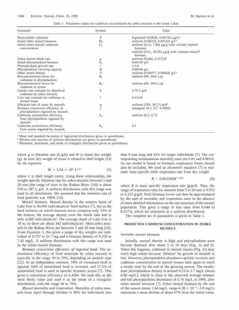
Initially, mussel density is high and phytoplankton soonbecome depleted after about 5 to 10 days (Fig. 1a and b).When this happens, cadmium in mussel tissues (Fig. 1c) mayreach high values because ‘dilution’ by growth of mussels islow. However, phytoplankton abundance quickly recovers andcadmium concentration in mussel tissues falls again to reacha steady state by the end of the growing season. The steady-state phytoplankton density is around 0.23 to 1.7 mg/L (mean0.98 mg/L), which is close to the observed average summerand fall phytoplankton abundance of 0.76 mg/L in 1990, afterzebra mussel invasion [7]. Zebra mussel biomass by the endof the season (mean 1.64 mg/L, range 6.38 3 10211–3.9 mg/L)represents a mean decline of about 67% from the initial value.


Fig. 1. Dynamics of phytoplankton (a), zebra mussels (b), and cad-mium in zebra mussels (c) in the western basin of Lake Erie, assumingbiomasses of zebra mussels and phytoplankton affect each other. Onethousand replicate simulations were run for 200 d each, with param-eters sampled at the start of each replicate. The bold line indicatesmean, the thin lines indicate the range on each graph.

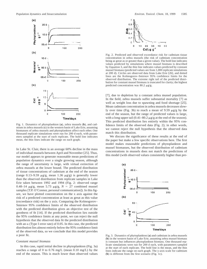
Fig. 2. Predicted and observed exceedance risk for cadmium tissueconcentration in zebra mussels (the risk of cadmium concentrationbeing as great as or greater than a given value). The bold line indicatesvalues predicted by simulations where mussel biomass is describedby Equation 3, and the thin line indicates values predicted by constantmussel biomass (predicted values are from 1,000 replicate simulationsat 200 d). Circles are observed data from Lake Erie [26], and dottedlines are the Kolmogorov–Smirnov 95% confidence limits for theobserved distribution. The extreme right tail of the predicted distri-bution for constant mussel biomass is truncated for clarity; the highestpredicted concentration was 80.2 mg/g.

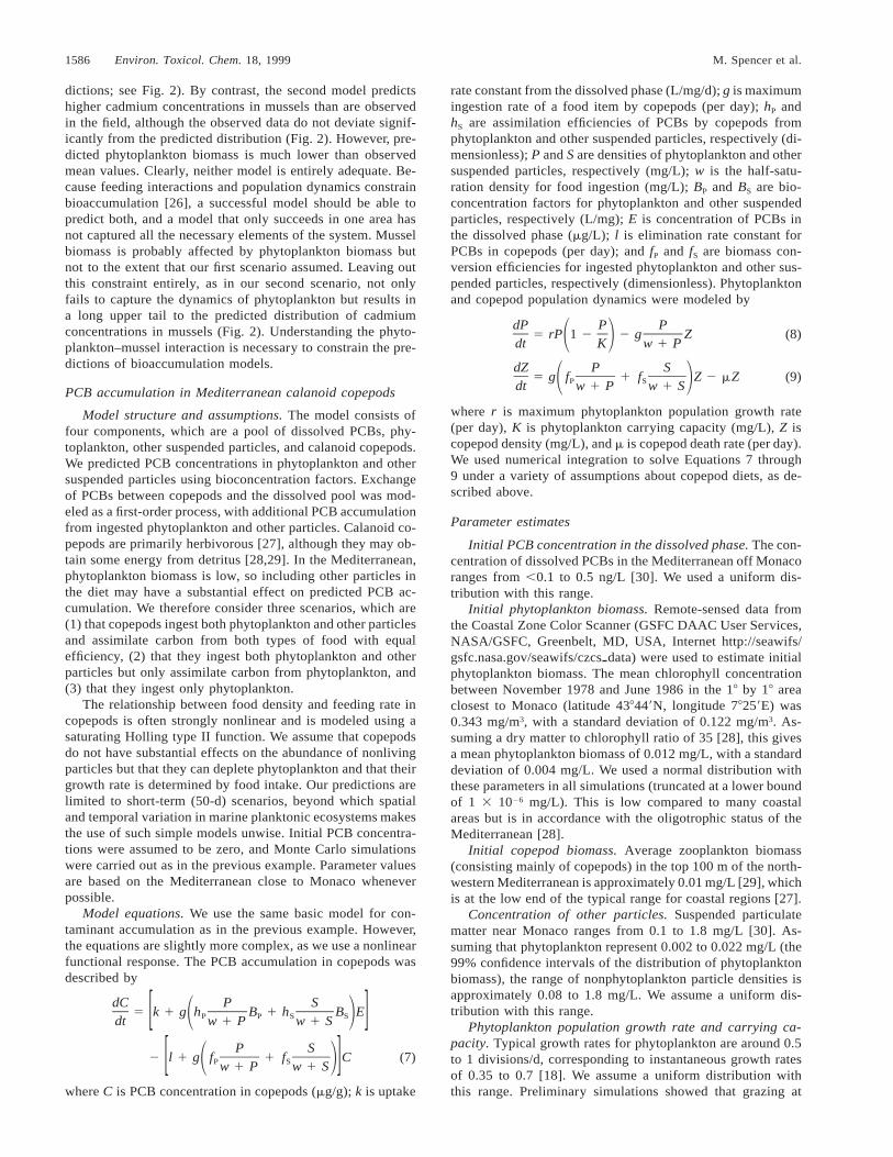
Fig. 3. Dynamics of phytoplankton (a) and cadmium in zebra mussels(b) in the western basin of Lake Erie, assuming zebra mussel biomassis constant but influences phytoplankton biomass. One thousand rep-licate simulations were run for 200 d each, with parameters sampledat the start of each replicate. The bold line is the mean, and the thinlines indicate the range on each graph. The y-axis scale for cadmium(b) is different from the first scenario (Fig. 1c).

In Lake St. Clair, there is an average 60% decline in the massof individual mussels between April and November [25]. Thus,our model appears to generate reasonable mean predictions ofpopulation dynamics over a single growing season, althoughthe range of uncertainty is large, with virtual extinction ofzebra mussels at the lower bound. The predicted distributionof tissue concentrations of cadmium at the end of the season(range 0.13–9.59 mg/g, mean 1.36 mg/g) is generally lowerthan the observed distribution from replicate samples in LakeErie taken between 1992 and 1994 (Fig. 2: observed range0.48–14 mg/g, mean 5.73 mg/g, N 5 27 combined musselsamples [T.P. O’Connor, personal communication]). In this fig-ure, we have plotted concentration on the x axis against therisk of a predicted concentration at least as great as this value(exceedance risk) on the y axis. Comparing the Kolmogorov–Smirnov 95% confidence limits of the observed distributionwith the predicted distribution gives an objective test of thegoodness of fit [14]. If the predicted distribution lies outsidethe 95% confidence limits at any point, we can reject the nullhypothesis that the observed data fit the predicted distributionwith an a (Type I error rate) of 0.05. In this case, the predicteddistribution lies almost entirely below the 95% confidence limitof the observed data, so we conclude that this model providesa poor fit.

Constant mussel biomass

In this case, rapid initial decline in phytoplankton (Fig. 3a)reaches a range of 0 to 0.76 mg/L (mean 0.10 mg/L) by theend of the season. This is much lower than observed values

[7], due to depletion by a constant zebra mussel population.In the field, zebra mussels suffer substantial mortality [7] aswell as weight loss due to spawning and food shortage [25].Mean cadmium concentration in zebra mussels decreases slow-ly over time (Fig. 3b) to reach a mean of 9.59 mg/g by theend of the season, but the range of predicted values is large,with a long upper tail (0.41–80.2 mg/g at the end of the season).This predicted distribution lies entirely within the 95% con-fidence limits of the observed data (Fig. 2); in other words,we cannot reject the null hypothesis that the observed datamatch this distribution.

We discuss the significance of these results at the end ofthe paper but make a few specific observations here. The firstmodel makes reasonable predictions of phytoplankton andmussel biomasses, but the observed distribution of cadmiumconcentrations in mussels does not match the predictions ofthis model (with observed values consistently higher than pre-


dictions; see Fig. 2). By contrast, the second model predictshigher cadmium concentrations in mussels than are observedin the field, although the observed data do not deviate signif-icantly from the predicted distribution (Fig. 2). However, pre-dicted phytoplankton biomass is much lower than observedmean values. Clearly, neither model is entirely adequate. Be-cause feeding interactions and population dynamics constrainbioaccumulation [26], a successful model should be able topredict both, and a model that only succeeds in one area hasnot captured all the necessary elements of the system. Musselbiomass is probably affected by phytoplankton biomass butnot to the extent that our first scenario assumed. Leaving outthis constraint entirely, as in our second scenario, not onlyfails to capture the dynamics of phytoplankton but results ina long upper tail to the predicted distribution of cadmiumconcentrations in mussels (Fig. 2). Understanding the phyto-plankton–mussel interaction is necessary to constrain the pre-dictions of bioaccumulation models.

PCB accumulation in Mediterranean calanoid copepods

Model structure and assumptions. The model consists offour components, which are a pool of dissolved PCBs, phy-toplankton, other suspended particles, and calanoid copepods.We predicted PCB concentrations in phytoplankton and othersuspended particles using bioconcentration factors. Exchangeof PCBs between copepods and the dissolved pool was mod-eled as a first-order process, with additional PCB accumulationfrom ingested phytoplankton and other particles. Calanoid co-pepods are primarily herbivorous [27], although they may ob-tain some energy from detritus [28,29]. In the Mediterranean,phytoplankton biomass is low, so including other particles inthe diet may have a substantial effect on predicted PCB ac-cumulation. We therefore consider three scenarios, which are(1) that copepods ingest both phytoplankton and other particlesand assimilate carbon from both types of food with equalefficiency, (2) that they ingest both phytoplankton and otherparticles but only assimilate carbon from phytoplankton, and(3) that they ingest only phytoplankton.

The relationship between food density and feeding rate incopepods is often strongly nonlinear and is modeled using asaturating Holling type II function. We assume that copepodsdo not have substantial effects on the abundance of nonlivingparticles but that they can deplete phytoplankton and that theirgrowth rate is determined by food intake. Our predictions arelimited to short-term (50-d) scenarios, beyond which spatialand temporal variation in marine planktonic ecosystems makesthe use of such simple models unwise. Initial PCB concentra-tions were assumed to be zero, and Monte Carlo simulationswere carried out as in the previous example. Parameter valuesare based on the Mediterranean close to Monaco wheneverpossible.

Model equations. We use the same basic model for con-taminant accumulation as in the previous example. However,the equations are slightly more complex, as we use a nonlinearfunctional response. The PCB accumulation in copepods wasdescribed by

dC P S5 k 1 g h B 1 h B EP P S S1 2[ ]dt w 1 P w 1 S

P S2 l 1 g f 1 f C (7)P S1 2[ ]w 1 P w 1 S

where C is PCB concentration in copepods (mg/g); k is uptake

rate constant from the dissolved phase (L/mg/d); g is maximumingestion rate of a food item by copepods (per day); hP andhS are assimilation efficiencies of PCBs by copepods fromphytoplankton and other suspended particles, respectively (di-mensionless); P and S are densities of phytoplankton and othersuspended particles, respectively (mg/L); w is the half-satu-ration density for food ingestion (mg/L); BP and BS are bio-concentration factors for phytoplankton and other suspendedparticles, respectively (L/mg); E is concentration of PCBs inthe dissolved phase (mg/L); l is elimination rate constant forPCBs in copepods (per day); and fP and fS are biomass con-version efficiencies for ingested phytoplankton and other sus-pended particles, respectively (dimensionless). Phytoplanktonand copepod population dynamics were modeled by

dP P P5 rP 1 2 2 g Z (8)1 2dt K w 1 P

dZ P S5 g f 1 f Z 2 mZ (9)P S1 2dt w 1 P w 1 S

where r is maximum phytoplankton population growth rate(per day), K is phytoplankton carrying capacity (mg/L), Z iscopepod density (mg/L), and m is copepod death rate (per day).We used numerical integration to solve Equations 7 through9 under a variety of assumptions about copepod diets, as de-scribed above.

Parameter estimates

Initial PCB concentration in the dissolved phase. The con-centration of dissolved PCBs in the Mediterranean off Monacoranges from ,0.1 to 0.5 ng/L [30]. We used a uniform dis-tribution with this range.

Initial phytoplankton biomass. Remote-sensed data fromthe Coastal Zone Color Scanner (GSFC DAAC User Services,NASA/GSFC, Greenbelt, MD, USA, Internet http://seawifs/gsfc.nasa.gov/seawifs/czcspdata) were used to estimate initialphytoplankton biomass. The mean chlorophyll concentrationbetween November 1978 and June 1986 in the 18 by 18 areaclosest to Monaco (latitude 438449N, longitude 78259E) was0.343 mg/m3, with a standard deviation of 0.122 mg/m3. As-suming a dry matter to chlorophyll ratio of 35 [28], this givesa mean phytoplankton biomass of 0.012 mg/L, with a standarddeviation of 0.004 mg/L. We used a normal distribution withthese parameters in all simulations (truncated at a lower boundof 1 3 1026 mg/L). This is low compared to many coastalareas but is in accordance with the oligotrophic status of theMediterranean [28].

Initial copepod biomass. Average zooplankton biomass(consisting mainly of copepods) in the top 100 m of the north-western Mediterranean is approximately 0.01 mg/L [29], whichis at the low end of the typical range for coastal regions [27].

Concentration of other particles. Suspended particulatematter near Monaco ranges from 0.1 to 1.8 mg/L [30]. As-suming that phytoplankton represent 0.002 to 0.022 mg/L (the99% confidence intervals of the distribution of phytoplanktonbiomass), the range of nonphytoplankton particle densities isapproximately 0.08 to 1.8 mg/L. We assume a uniform dis-tribution with this range.

Phytoplankton population growth rate and carrying ca-pacity. Typical growth rates for phytoplankton are around 0.5to 1 divisions/d, corresponding to instantaneous growth ratesof 0.35 to 0.7 [18]. We assume a uniform distribution withthis range. Preliminary simulations showed that grazing at


Table 2. Parameter values for PCB accumulation by copepods in the Mediterranean

Parameter Symbol Value

Dissolved PCBInitial copepod biomassCopepod death rateInitial phytoplankton biomassPhytoplankton growth ratePhytoplankton carrying capacityBiomass of other particles

EZ0

mP0

rKS

uniform (0.0001, 0.0005) mg/La

0.01 mg/Luniform (0.04, 0.13)/da

lower-truncated normal (0.012, 0.004, 1E26) mg/Lb

uniform (0.35, 0.7)/dlower-truncated normal (0.012, 0.004, 1E26) mg/Lb

uniform (0.08, 1.8) mg/La

Bioconcentration factor for PCBs inphytoplankton

BP 0.1 L/mg

Bioconcentration factor for PCBs inother particles

BS uniform (0.26, 1.3) L/mga

Uptake rate constant for dissolvedPCBs by copepods

k 0.073 L/mg/d

Loss rate constant for PCBs in copepodtissue

l uniform (0.144, 0.272)/da

Maximum copepod feeding rateHalf-saturation density for copepod

feeding

gw

0.192/d (or 0/d for other particles in scenario 3)0.1 mg/L

Biomass conversion efficiency forphytoplankton ingested by copepods

fP uniform (0.5, 0.8)a

Biomass conversion efficiency for otherparticles ingested by copepods

fS uniform (0.5, 0.8) or 0 in scenario 2a

PCB assimilation efficiency fromphytoplankton ingested by copepods

hP uniform (0.37, 0.45)a

PCB assimilation efficiency from otherparticles ingested by copepods

hS uniform (0.37, 0.45)a

a Minima and maxima of uniform distributions are given in parentheses.b Mean, standard deviation, and truncation bound of lower-truncated normal distributions are given in parentheses.

realistic zooplankton biomasses had little effect on phyto-plankton biomass. We therefore used the observed long-termaverage phytoplankton biomass (0.012 mg/L, with a standarddeviation of 0.004 mg/L assumed to be normally distributedand truncated at a lower bound of 1 3 1026 mg/L) as anapproximation to phytoplankton carrying capacity.

PCB accumulation in phytoplankton and other particles.Bioconcentration factors for PCBs in marine phytoplanktonaverage about 100 L/g [31,32]. Nonliving particles collectedin sediment traps off Monaco contained 130 ng/g PCBs [30],giving a BCF of 0.26 to 1.3 L/mg. We assumed a uniformdistribution with this range for other particles.

Uptake and elimination of PCBs from water and food bycopepods. Uptake of 14C-labeled 2,29,4,49-tetrachlorobiphenylby copepods from the dissolved phase is 0.073 L/mg/d [32].The assimilation efficiency of radiolabelled 2,29,4,49-tetrach-lorobiphenyl by marine copepods (Acartia tonsa and Temoralongicornis) feeding on the diatom Thalassiosira pseudonanaranged between 0.37 and 0.45 [32]. We used a uniform dis-tribution with this range for assimilation from both phyto-plankton and other particles. Depuration of radiolabeled 14CPCB following uptake from the dissolved phase or food rangedbetween 0.144 and 0.272/d [32]. We used a uniform distri-bution with this range for the elimination rate constant.

Conversion efficiency of ingested food. Conversion effi-ciency of ingested phytoplankton by copepods is generally inthe range 0.5 to 0.8 [33] and is relatively independent of foodquantity and quality. Conversion efficiency of other particlesis less well known, so we assume either that it is the same asfor phytoplankton (scenario 1) or that it is zero (scenario 2).

Feeding rate of copepods. Feeding rates of continuouslyfeeding copepods at a range of phytoplankton densities (ex-pressed in mg carbon/L)can be predicted by a relationship ofthe form

I 5 Im (1 2 e2d(P2P9)) (10)

[27] where I is ingestion rate (per hour), Im is maximum in-gestion rate (per hour), d is a constant defining the rate ofchange of ingestion with food concentration, P is food con-centration (mg carbon/L), and P9 is the minimum food con-centration at which ingestion will occur (mg carbon/L). Fittedparameters are Im 5 0.008/h, P9 5 15 mg C/L, and d 5 0.0140[34]. This relationship can be approximated by a Holling typeII function with g 5 0.192/d and w 5 0.1 mg/L, assuming acarbon:dry mass ratio of 0.5. We assume either that this feedingrate applies to both phytoplankton and other particles (sce-narios 1 and 2) or that there is no feeding on nonliving particles(scenario 3).

Death rate of copepods. Death rates of A. tonsa with 0.1to 0.4 mg/L of diatom food in filtered seawater with addeddetritus were 0.04 to 0.13/d [29]. We used a uniform distri-bution with this range.

The complete set of parameters is given in Table 2.

PREDICTED PCB CONCENTRATION IN CALANOIDCOPEPODS

Detritus ingested and carbon from detritus assimilated

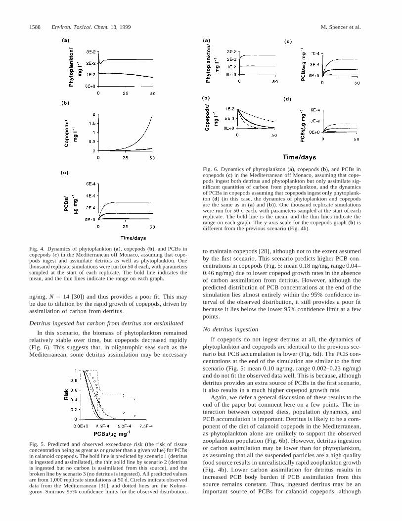
Over 50 d, phytoplankton biomass decreased slightly butcopepod biomass increased rapidly (Fig. 4). The final copepodbiomass was about 10 times higher than typical values for theMediterranean. This suggests either that phytoplankton patchesare unlikely to persist for as long as 50 d or that feeding andassimilation rates for detritus are lower than this model as-sumes. The PCB concentration in copepods attained a steadystate by the end of the simulation (Fig. 5: mean 0.1 ng/mg,range 0.002–0.30 ng/mg), but the distribution of predicted con-centrations lies almost entirely below the 95% confidence limitfor the observed data (mean 0.23 ng/mg, range 0.07–0.62


Fig. 4. Dynamics of phytoplankton (a), copepods (b), and PCBs incopepods (c) in the Mediterranean off Monaco, assuming that cope-pods ingest and assimilate detritus as well as phytoplankton. Onethousand replicate simulations were run for 50 d each, with parameterssampled at the start of each replicate. The bold line indicates themean, and the thin lines indicate the range on each graph.

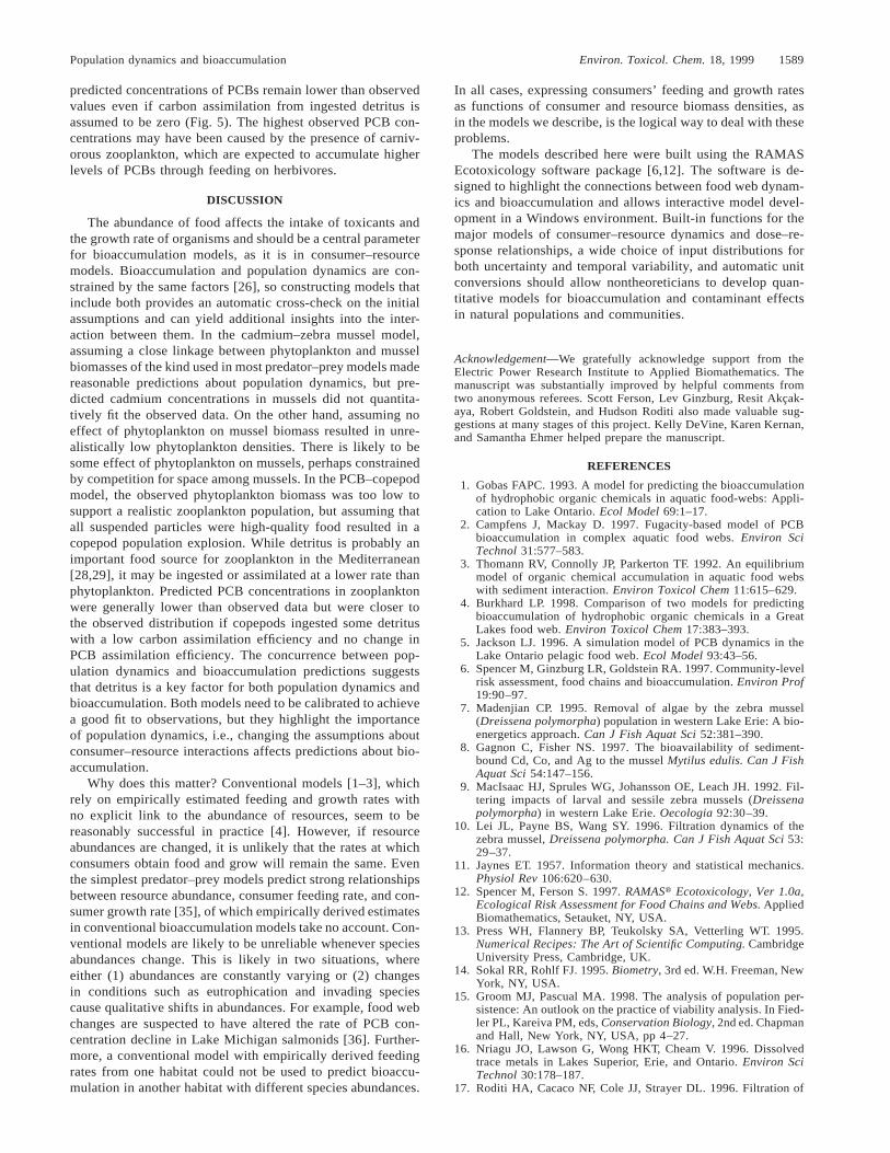
Fig. 6. Dynamics of phytoplankton (a), copepods (b), and PCBs incopepods (c) in the Mediterranean off Monaco, assuming that cope-pods ingest both detritus and phytoplankton but only assimilate sig-nificant quantities of carbon from phytoplankton, and the dynamicsof PCBs in copepods assuming that copepods ingest only phytoplank-ton (d) (in this case, the dynamics of phytoplankton and copepodsare the same as in (a) and (b)). One thousand replicate simulationswere run for 50 d each, with parameters sampled at the start of eachreplicate. The bold line is the mean, and the thin lines indicate therange on each graph. The y-axis scale for the copepods graph (b) isdifferent from the previous scenario (Fig. 4b).

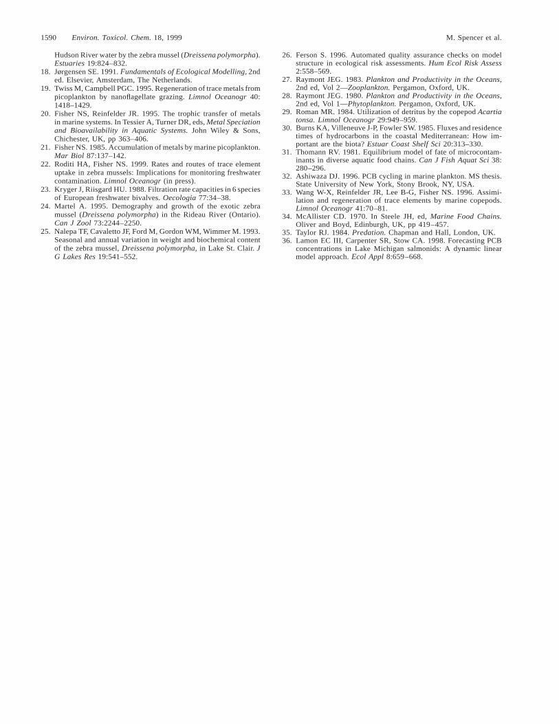
Fig. 5. Predicted and observed exceedance risk (the risk of tissueconcentration being as great as or greater than a given value) for PCBsin calanoid copepods. The bold line is predicted by scenario 1 (detritusis ingested and assimilated), the thin solid line by scenario 2 (detritusis ingested but no carbon is assimilated from this source), and thebroken line by scenario 3 (no detritus is ingested). All predicted valuesare from 1,000 replicate simulations at 50 d. Circles indicate observeddata from the Mediterranean [31], and dotted lines are the Kolmo-gorov–Smirnov 95% confidence limits for the observed distribution.

ng/mg, N 5 14 [30]) and thus provides a poor fit. This maybe due to dilution by the rapid growth of copepods, driven byassimilation of carbon from detritus.

Detritus ingested but carbon from detritus not assimilated

In this scenario, the biomass of phytoplankton remainedrelatively stable over time, but copepods decreased rapidly(Fig. 6). This suggests that, in oligotrophic seas such as theMediterranean, some detritus assimilation may be necessary

to maintain copepods [28], although not to the extent assumedby the first scenario. This scenario predicts higher PCB con-centrations in copepods (Fig. 5: mean 0.18 ng/mg, range 0.04–0.46 ng/mg) due to lower copepod growth rates in the absenceof carbon assimilation from detritus. However, although thepredicted distribution of PCB concentrations at the end of thesimulation lies almost entirely within the 95% confidence in-terval of the observed distribution, it still provides a poor fitbecause it lies below the lower 95% confidence limit at a fewpoints.

No detritus ingestion

If copepods do not ingest detritus at all, the dynamics ofphytoplankton and copepods are identical to the previous sce-nario but PCB accumulation is lower (Fig. 6d). The PCB con-centrations at the end of the simulation are similar to the firstscenario (Fig. 5: mean 0.10 ng/mg, range 0.002–0.23 ng/mg)and do not fit the observed data well. This is because, althoughdetritus provides an extra source of PCBs in the first scenario,it also results in a much higher copepod growth rate.

Again, we defer a general discussion of these results to theend of the paper but comment here on a few points. The in-teraction between copepod diets, population dynamics, andPCB accumulation is important. Detritus is likely to be a com-ponent of the diet of calanoid copepods in the Mediterranean,as phytoplankton alone are unlikely to support the observedzooplankton population (Fig. 6b). However, detritus ingestionor carbon assimilation may be lower than for phytoplankton,as assuming that all the suspended particles are a high qualityfood source results in unrealistically rapid zooplankton growth(Fig. 4b). Lower carbon assimilation for detritus results inincreased PCB body burden if PCB assimilation from thissource remains constant. Thus, ingested detritus may be animportant source of PCBs for calanoid copepods, although


predicted concentrations of PCBs remain lower than observedvalues even if carbon assimilation from ingested detritus isassumed to be zero (Fig. 5). The highest observed PCB con-centrations may have been caused by the presence of carniv-orous zooplankton, which are expected to accumulate higherlevels of PCBs through feeding on herbivores.

DISCUSSION

The abundance of food affects the intake of toxicants andthe growth rate of organisms and should be a central parameterfor bioaccumulation models, as it is in consumer–resourcemodels. Bioaccumulation and population dynamics are con-strained by the same factors [26], so constructing models thatinclude both provides an automatic cross-check on the initialassumptions and can yield additional insights into the inter-action between them. In the cadmium–zebra mussel model,assuming a close linkage between phytoplankton and musselbiomasses of the kind used in most predator–prey models madereasonable predictions about population dynamics, but pre-dicted cadmium concentrations in mussels did not quantita-tively fit the observed data. On the other hand, assuming noeffect of phytoplankton on mussel biomass resulted in unre-alistically low phytoplankton densities. There is likely to besome effect of phytoplankton on mussels, perhaps constrainedby competition for space among mussels. In the PCB–copepodmodel, the observed phytoplankton biomass was too low tosupport a realistic zooplankton population, but assuming thatall suspended particles were high-quality food resulted in acopepod population explosion. While detritus is probably animportant food source for zooplankton in the Mediterranean[28,29], it may be ingested or assimilated at a lower rate thanphytoplankton. Predicted PCB concentrations in zooplanktonwere generally lower than observed data but were closer tothe observed distribution if copepods ingested some detrituswith a low carbon assimilation efficiency and no change inPCB assimilation efficiency. The concurrence between pop-ulation dynamics and bioaccumulation predictions suggeststhat detritus is a key factor for both population dynamics andbioaccumulation. Both models need to be calibrated to achievea good fit to observations, but they highlight the importanceof population dynamics, i.e., changing the assumptions aboutconsumer–resource interactions affects predictions about bio-accumulation.

Why does this matter? Conventional models [1–3], whichrely on empirically estimated feeding and growth rates withno explicit link to the abundance of resources, seem to bereasonably successful in practice [4]. However, if resourceabundances are changed, it is unlikely that the rates at whichconsumers obtain food and grow will remain the same. Eventhe simplest predator–prey models predict strong relationshipsbetween resource abundance, consumer feeding rate, and con-sumer growth rate [35], of which empirically derived estimatesin conventional bioaccumulation models take no account. Con-ventional models are likely to be unreliable whenever speciesabundances change. This is likely in two situations, whereeither (1) abundances are constantly varying or (2) changesin conditions such as eutrophication and invading speciescause qualitative shifts in abundances. For example, food webchanges are suspected to have altered the rate of PCB con-centration decline in Lake Michigan salmonids [36]. Further-more, a conventional model with empirically derived feedingrates from one habitat could not be used to predict bioaccu-mulation in another habitat with different species abundances.

In all cases, expressing consumers’ feeding and growth ratesas functions of consumer and resource biomass densities, asin the models we describe, is the logical way to deal with theseproblems.

The models described here were built using the RAMASEcotoxicology software package [6,12]. The software is de-signed to highlight the connections between food web dynam-ics and bioaccumulation and allows interactive model devel-opment in a Windows environment. Built-in functions for themajor models of consumer–resource dynamics and dose–re-sponse relationships, a wide choice of input distributions forboth uncertainty and temporal variability, and automatic unitconversions should allow nontheoreticians to develop quan-titative models for bioaccumulation and contaminant effectsin natural populations and communities.

Acknowledgement—We gratefully acknowledge support from theElectric Power Research Institute to Applied Biomathematics. Themanuscript was substantially improved by helpful comments fromtwo anonymous referees. Scott Ferson, Lev Ginzburg, Resit Akcak-aya, Robert Goldstein, and Hudson Roditi also made valuable sug-gestions at many stages of this project. Kelly DeVine, Karen Kernan,and Samantha Ehmer helped prepare the manuscript.

REFERENCES

1. Gobas FAPC. 1993. A model for predicting the bioaccumulationof hydrophobic organic chemicals in aquatic food-webs: Appli-cation to Lake Ontario. Ecol Model 69:1–17.

2. Campfens J, Mackay D. 1997. Fugacity-based model of PCBbioaccumulation in complex aquatic food webs. Environ SciTechnol 31:577–583.

3. Thomann RV, Connolly JP, Parkerton TF. 1992. An equilibriummodel of organic chemical accumulation in aquatic food webswith sediment interaction. Environ Toxicol Chem 11:615–629.

4. Burkhard LP. 1998. Comparison of two models for predictingbioaccumulation of hydrophobic organic chemicals in a GreatLakes food web. Environ Toxicol Chem 17:383–393.

5. Jackson LJ. 1996. A simulation model of PCB dynamics in theLake Ontario pelagic food web. Ecol Model 93:43–56.

6. Spencer M, Ginzburg LR, Goldstein RA. 1997. Community-levelrisk assessment, food chains and bioaccumulation. Environ Prof19:90–97.

7. Madenjian CP. 1995. Removal of algae by the zebra mussel(Dreissena polymorpha) population in western Lake Erie: A bio-energetics approach. Can J Fish Aquat Sci 52:381–390.

8. Gagnon C, Fisher NS. 1997. The bioavailability of sediment-bound Cd, Co, and Ag to the mussel Mytilus edulis. Can J FishAquat Sci 54:147–156.

9. MacIsaac HJ, Sprules WG, Johansson OE, Leach JH. 1992. Fil-tering impacts of larval and sessile zebra mussels (Dreissenapolymorpha) in western Lake Erie. Oecologia 92:30–39.

10. Lei JL, Payne BS, Wang SY. 1996. Filtration dynamics of thezebra mussel, Dreissena polymorpha. Can J Fish Aquat Sci 53:29–37.

11. Jaynes ET. 1957. Information theory and statistical mechanics.Physiol Rev 106:620–630.

12. Spencer M, Ferson S. 1997. RAMASt Ecotoxicology, Ver 1.0a,Ecological Risk Assessment for Food Chains and Webs. AppliedBiomathematics, Setauket, NY, USA.

13. Press WH, Flannery BP, Teukolsky SA, Vetterling WT. 1995.Numerical Recipes: The Art of Scientific Computing. CambridgeUniversity Press, Cambridge, UK.

14. Sokal RR, Rohlf FJ. 1995. Biometry, 3rd ed. W.H. Freeman, NewYork, NY, USA.

15. Groom MJ, Pascual MA. 1998. The analysis of population per-sistence: An outlook on the practice of viability analysis. In Fied-ler PL, Kareiva PM, eds, Conservation Biology, 2nd ed. Chapmanand Hall, New York, NY, USA, pp 4–27.

16. Nriagu JO, Lawson G, Wong HKT, Cheam V. 1996. Dissolvedtrace metals in Lakes Superior, Erie, and Ontario. Environ SciTechnol 30:178–187.

17. Roditi HA, Cacaco NF, Cole JJ, Strayer DL. 1996. Filtration of


Hudson River water by the zebra mussel (Dreissena polymorpha).Estuaries 19:824–832.

18. Jørgensen SE. 1991. Fundamentals of Ecological Modelling, 2nded. Elsevier, Amsterdam, The Netherlands.

19. Twiss M, Campbell PGC. 1995. Regeneration of trace metals frompicoplankton by nanoflagellate grazing. Limnol Oceanogr 40:1418–1429.

20. Fisher NS, Reinfelder JR. 1995. The trophic transfer of metalsin marine systems. In Tessier A, Turner DR, eds, Metal Speciationand Bioavailability in Aquatic Systems. John Wiley & Sons,Chichester, UK, pp 363–406.

21. Fisher NS. 1985. Accumulation of metals by marine picoplankton.Mar Biol 87:137–142.

22. Roditi HA, Fisher NS. 1999. Rates and routes of trace elementuptake in zebra mussels: Implications for monitoring freshwatercontamination. Limnol Oceanogr (in press).

23. Kryger J, Riisgard HU. 1988. Filtration rate capacities in 6 speciesof European freshwater bivalves. Oecologia 77:34–38.

24. Martel A. 1995. Demography and growth of the exotic zebramussel (Dreissena polymorpha) in the Rideau River (Ontario).Can J Zool 73:2244–2250.

25. Nalepa TF, Cavaletto JF, Ford M, Gordon WM, Wimmer M. 1993.Seasonal and annual variation in weight and biochemical contentof the zebra mussel, Dreissena polymorpha, in Lake St. Clair. JG Lakes Res 19:541–552.

26. Ferson S. 1996. Automated quality assurance checks on modelstructure in ecological risk assessments. Hum Ecol Risk Assess2:558–569.

27. Raymont JEG. 1983. Plankton and Productivity in the Oceans,2nd ed, Vol 2—Zooplankton. Pergamon, Oxford, UK.

28. Raymont JEG. 1980. Plankton and Productivity in the Oceans,2nd ed, Vol 1—Phytoplankton. Pergamon, Oxford, UK.

29. Roman MR. 1984. Utilization of detritus by the copepod Acartiatonsa. Limnol Oceanogr 29:949–959.

30. Burns KA, Villeneuve J-P, Fowler SW. 1985. Fluxes and residencetimes of hydrocarbons in the coastal Mediterranean: How im-portant are the biota? Estuar Coast Shelf Sci 20:313–330.

31. Thomann RV. 1981. Equilibrium model of fate of microcontam-inants in diverse aquatic food chains. Can J Fish Aquat Sci 38:280–296.

32. Ashiwaza DJ. 1996. PCB cycling in marine plankton. MS thesis.State University of New York, Stony Brook, NY, USA.

33. Wang W-X, Reinfelder JR, Lee B-G, Fisher NS. 1996. Assimi-lation and regeneration of trace elements by marine copepods.Limnol Oceanogr 41:70–81.

34. McAllister CD. 1970. In Steele JH, ed, Marine Food Chains.Oliver and Boyd, Edinburgh, UK, pp 419–457.

35. Taylor RJ. 1984. Predation. Chapman and Hall, London, UK.36. Lamon EC III, Carpenter SR, Stow CA. 1998. Forecasting PCB

concentrations in Lake Michigan salmonids: A dynamic linearmodel approach. Ecol Appl 8:659–668.

Documents

Exploring the effects of consumer–resource dynamics on contaminant bioaccumulation by aquatic herbivores