University of Central Florida University of Central Florida

STARS STARS

Electronic Theses and Dissertations, 2004-2019

2011

Exploring Techniques For Measurement And Improvement Of Exploring Techniques For Measurement And Improvement Of

Data Quality With Application To Determination Of The Last Data Quality With Application To Determination Of The Last

Known Position (lkp) In Search And Rescue (sar) Data Known Position (lkp) In Search And Rescue (sar) Data

Abhijit Wakchaure University of Central Florida

Part of the Electrical and Electronics Commons

Find similar works at: https://stars.library.ucf.edu/etd

University of Central Florida Libraries http://library.ucf.edu

This Doctoral Dissertation (Open Access) is brought to you for free and open access by STARS. It has been accepted

for inclusion in Electronic Theses and Dissertations, 2004-2019 by an authorized administrator of STARS. For more

information, please contact STARS@ucf.edu.

STARS Citation STARS Citation Wakchaure, Abhijit, "Exploring Techniques For Measurement And Improvement Of Data Quality With Application To Determination Of The Last Known Position (lkp) In Search And Rescue (sar) Data" (2011). Electronic Theses and Dissertations, 2004-2019. 1812. https://stars.library.ucf.edu/etd/1812

EXPLORING TECHNIQUES FOR MEASUREMENT AND IMPROVEMENT OF DATA QUALITY WITH APPLICATION TO DETERMINATION OF THE LAST KNOWN POSITION (LKP) IN

SEARCH AND RESCUE (SAR) DATA

by

ABHIJIT WAKCHAURE M.S. University of Central Florida, 2002

A dissertation submitted in partial fulfillment of the requirements for the degree of Doctor of Philosophy

in the Department of Electrical Engineering and Computer Science in the College of Engineering & Computer Science

at the University of Central Florida Orlando, Florida

Summer Term 2011

Major Professor: Kien Hua

ii

©2011 Abhijit Wakchaure

iii

ABSTRACT

There is a tremendous volume of data being generated in today’s world. As organizations around the globe realize the increased importance of their data as being a valuable asset in gaining a competitive edge in a fast-paced and a dynamic business world, more and more attention is being paid to the quality of the data. Advances in the fields of data mining, predictive modeling, text mining, web mining, business intelligence, health care analytics, etc. all depend on clean, accurate data. That one cannot effectively mine data, which is dirty, comes as no surprise. This research is an exploratory study of different domain data sets, addressing the data quality issues specific to each domain, identifying the challenges faced and arriving at techniques or methodologies for measuring and improving the data quality. The primary focus of the research is on the SAR or Search and Rescue dataset, identifying key issues related to data quality therein and developing an algorithm for improving the data quality. SAR missions which are routinely conducted all over the world show a trend of increasing mission costs. Retrospective studies of historic SAR data not only allow for a detailed analysis and understanding of SAR incidents and patterns, but also form the basis for generating probability maps, analytical data models, etc., which allow for an efficient use of valuable SAR resources and their distribution. One of the challenges with regards to the SAR dataset is that the collection process is not perfect. Often, the LKP or the Last Known Position is not known or cannot be arrived at. The goal is to fully or partially geocode the LKP for as many data points as possible, identify those data points where the LKP cannot be geocoded at all, and further highlight the underlying data quality issues. The SAR Algorithm has been developed, which makes use of partial or incomplete information, cleans and validates the data, and further extracts address information from relevant fields to successfully geocode the data. The algorithm improves the geocoding accuracy and has been validated by a set of approaches.

iv

ACKNOWLEDGMENTS

First of all, I wish to genuinely and sincerely thank Dr. Ron Eaglin for his guidance, advice and support throughout this journey. I am truly grateful to have had the opportunity to work with him and he is indeed a true inspiration. I also warmly wish to extend my gratitude to Dr. Kien Hua, who has always been really helpful, very supportive and has offered valuable feedback in my work. I am greatly thankful to Dr. Michael Georgiopoulos, Dr. Bahman Motlagh and Dr. Cliff Zou for their valuable comments, scholarly advice and constructive criticism during the course of my study. I take this opportunity to sincerely thank the EECS Department, especially Dr. Ronald DeMara and Dr. Charles Reilly from the Office of Academic Affairs, for their help and support. I also am very thankful to Ms. Heather Stevens, Ms. Nicole Mitchell and Ms. Grissel Guzman for their help. I wish to extend my thanks to Dr. Karla Moore in her role as a Project Manager for some of the projects I worked on. I am also thankful towards Ms. June Wingler and Ms. Ronee Trantham for always providing the administrative help. I truly feel thankful to all the great teachers I have had all along, which made learning a lot interesting. Finally, I owe a special thanks to my parents and my sister for their love, encouragement and unwavering support always, without which I would never have reached this stage in my life. I also appreciate my luck in having great friends and well-wishers along the way, which makes any journey truly worthwhile.

v

TABLE OF CONTENTS

LIST OF FIGURES ............................................................................................................................ viii

LIST OF TABLES ................................................................................................................................ ix

CHAPTER 1: INTRODUCTION ........................................................................................................... 1

Research Aim ............................................................................................................................... 5

Research Objectives .................................................................................................................... 5

Methodology ............................................................................................................................... 6

CHAPTER 2: LITERATURE REVIEW ................................................................................................... 8

CHAPTER 3: DATA QUALITY WORK IN DIFFERENT DATA DOMAINS ............................................. 18

Data Cleanliness techniques as applied to Seminole County Address data ............................. 18

Introduction ........................................................................................................................... 18

Overview of the Address Data ............................................................................................... 18

Cleaning Phases ..................................................................................................................... 19

Simple Clean .......................................................................................................................... 20

Simple Clean Summary .......................................................................................................... 22

Final Clean .............................................................................................................................. 24

ANSWER Algorithm on the FINDER Data .................................................................................. 24

Measuring Data Cleanliness for Person Data ............................................................................ 27

Motivation ............................................................................................................................. 28

Procedure .............................................................................................................................. 30

Data-Cleanliness algorithm.................................................................................................... 31

Basis for 85% threshold ......................................................................................................... 32

How run variations were achieved – significance of weights – justification ........................ 32

Results .................................................................................................................................... 33

Conclusion & Future Work .................................................................................................... 39

Data Validation of a Vehicle Identification Number (VIN) Dataset........................................... 40

The Need for Data Validation ................................................................................................ 41

Our Approach ........................................................................................................................ 45

vi

Conclusions ............................................................................................................................ 48

CHAPTER 4: INTRODUCTION TO SEARCH AND RESCUE (SAR) DATA ............................................ 50

Geocoding ................................................................................................................................. 55

Different levels of Geocoding .................................................................................................... 56

The Google Geocoding API ........................................................................................................ 57

Geocoding as applied to the SAR dataset ................................................................................. 58

The GNIS Database .................................................................................................................... 59

The SAR Dataset ........................................................................................................................ 61

CHAPTER 5: SAR ALGORITHM – APPROACH, ANALYSIS & RESULTS ............................................. 70

When address fields have been populated............................................................................... 72

When address fields alone prove insufficient ........................................................................... 74

Where the records are unable to be geocoded ........................................................................ 75

When LKP coordinates have been specified ............................................................................. 76

SAR Algorithm flowcharts ......................................................................................................... 77

Results for some of the Table Categories ................................................................................. 99

Validating the SAR Algorithm .................................................................................................. 103

CHAPTER 6: FINDINGS & DISCUSSION ........................................................................................ 111

Challenges faced in the SAR Study .......................................................................................... 111

Geocoding Accuracy Output Approach for validating the SAR algorithm .............................. 116

Validation Process ................................................................................................................... 118

SAR Algorithm Analysis ........................................................................................................... 125

Validating the 'City'(C) field ................................................................................................. 125

Validating the 'County'(K) field ............................................................................................ 125

Extracting Feature Names(FNA) from the 'Comments' field ............................................... 125

Extracting Feature Names(FNB) from the 'LKP Type' field .................................................. 126

Extracting Street address information from the 'Comments' field ..................................... 126

Extracting Street address information from the 'LKP Type' field ........................................ 127

Results and Discussion ............................................................................................................ 127

Improving the SAR Algorithm Accuracy............................................................................... 128

vii

Findings from Data Quality Work in Other Domains .............................................................. 129

Business Logic framework for the Vehicle Identification Number (VIN) ............................ 130

Technique for Measuring Data Quality of Person Names as applied to Pawn data ........... 131

Data Cleanliness Techniques applied to the Seminole County Address data ..................... 132

String Matching Algorithm as applied to Burglary data ...................................................... 133

Relevance of this Study ........................................................................................................... 134

Future Work ............................................................................................................................ 135

REFERENCES ................................................................................................................................ 137

viii

LIST OF FIGURES

Figure 1 The tree obtained by insertion of 'John','Jon','Jonathan','Olcay','Jim','Oclay' and 'Jimmy' .......... 26 Figure 3 Data Validation implementation using Regular Expression Validators, highlighting any data errors ........................................................................................................................................................... 48 Figure 4 SAR Operations by Year ................................................................................................................ 51 Figure 5 Flowchart for the SAR Algorithm .................................................................................................. 79 Figure 6 Flowchart component for 'Plotting and Validation' ...................................................................... 81 Figure 7 Flowchart component for ‘County’ ............................................................................................... 82 Figure 8 Flowchart path 1-3-4-12-25-26-31 ................................................................................................ 84 Figure 9 Detailed Flowchart for 'Plotting and Validation' ........................................................................... 87 Figure 10 Detailed Flowchart for Invalid County ........................................................................................ 90 Figure 11 Examples of invalid counties in the SAR dataset ........................................................................ 91 Figure 12 Detailed Flowchart for Invalid City .............................................................................................. 94 Figure 13 Examples of invalid cities in the SAR dataset .............................................................................. 95 Figure 14 Instance of a False Positive for the Table 4a ............................................................................. 101 Figure 15 Validation sample Original and Calculated Coordinates plotted in Google Earth .................... 109 Figure 16 SAR Algorithm Geocodable break-up of records for the Validation sample ............................ 110 Figure 17 Geocoding 'Alafaya Trail, Orlando, FL' ...................................................................................... 112 Figure 18 Geocoding 'SR 434, Orlando, FL' ............................................................................................... 113 Figure 19 Geocoding 'State Road 434, Orlando, FL' ................................................................................. 113

ix

LIST OF TABLES Table 1 Data quality summary for the simple clean phase ......................................................................... 23 Table 2 Example of an intermediate table generated by the procedure ................................................... 35 Table 3 Intermediate table depicting variation in date of birth ................................................................. 35 Table 4 Example of name variation in last name ........................................................................................ 36 Table 5 Example of multiple variation ........................................................................................................ 37 Table 6 Database table showing Regular Expression rules and their descriptions..................................... 46 Table 7 SAR Statistics highlighting the rising costs of SAR Operations ....................................................... 52 Table 8 Sample records for the GNIS Database .......................................................................................... 60 Table 9 Sample records for the SAR Dataset columns 1 through 8 ............................................................ 63 Table 10 Sample records for the SAR Dataset columns 9 through 15 ........................................................ 63 Table 11 Sample records for the SAR Dataset columns 16 through 25 ...................................................... 63 Table 12 Sample records for the SAR Dataset columns 26 through 34 ...................................................... 63 Table 13 Sample records for the SAR Dataset columns 35 through 39 ...................................................... 63 Table 14 Sample records for the SAR Dataset columns 40 through 49 ...................................................... 63 Table 15 Sample records for the SAR Dataset columns 50 through 57 ...................................................... 63 Table 16 Sample records for the SAR Dataset columns 58 through 63 ...................................................... 64 Table 17 Sample records for the SAR Dataset columns 64 through 70 ...................................................... 64 Table 18 Sample records for the SAR Dataset columns 71 through 77 ...................................................... 64 Table 19 Sample records for the SAR Dataset column 78 .......................................................................... 64 Table 20 SAR Data subset containing fields important for geocoding ....................................................... 65 Table 21 Examples of variations in coordinate formats for Australia ........................................................ 65 Table 22 Examples of variations in coordinate formats for Canada ........................................................... 65 Table 23 Examples of variations in coordinate formats for New Zealand .................................................. 66 Table 24 Examples of variations in coordinate formats for Arizona, US .................................................... 66 Table 25 Examples of variations in coordinate formats for New Jersey and New York, US ....................... 66 Table 26 Examples of variations in coordinate formats for New York, US ................................................. 66 Table 27 Variation in coordinate formats across the US state of Washington ........................................... 67 Table 28 SAR Data subset highlighting the [LKP Type] field ....................................................................... 67 Table 29 Data in the 'comments' field ........................................................................................................ 68 Table 30 Mapped table categories ............................................................................................................. 97 Table 31 Category table 4a Geocoding Results .......................................................................................... 99 Table 32 Results for Category table 1a part1 ........................................................................................... 102 Table 33 Results for Category table 1a part2 ........................................................................................... 103 Table 34 Examples of Invalid counties in the Validation Sample.............................................................. 105 Table 35 Examples of Feature names extracted from Comments for the Validation Sample ................. 106 Table 36 Examples of Feature names extracted from LKP Type for the Validation Sample..................... 107 Table 37 Examples of Street Address information extracted from Comments for the Validation Sample .................................................................................................................................................................. 107

x

Table 38 Examples of Street Address information extracted from LKP Type for the Validation Sample . 108 Table 39 Extracting street address information ....................................................................................... 114 Table 40 Levels of Geocoding Accuracy .................................................................................................... 118 Table 41 Validating the 'City'(C) field ........................................................................................................ 120 Table 42 Validating the 'County'(K) field .................................................................................................. 120 Table 43 Extracting Feature Names(FNA) from the 'Comments' field...................................................... 121 Table 44 Extracting Feature Names(FNB) from the 'LKP Type' field ......................................................... 122 Table 45 Extracting Street address information(SA) from the 'Comments' field ..................................... 123 Table 46 Extracting Street address information(SB) from the 'LKP Type' field ........................................ 124

1

CHAPTER 1: INTRODUCTION

The volume of data in today’s world is growing rapidly. As organizations around the globe

realize the increased importance of their data as being a valuable asset in giving them the

competitive edge in today’s fast-paced business world, more and more attention is being paid

to the quality of this data. The data explosion phenomenon has created an immense

opportunity and the need for methodologies of Knowledge Discovery and Data Mining (KDD)

(IBM Research, n. d.). Data mining has become a very promising and a lucrative field, and is

emerging as one of the top key technology areas in information and knowledge management.

Organizations are building data repositories and data warehouses so as to effectively mine data

and extract meaningful context-based information out of available data.

Recent reports by IDC (Benchmark, 2006) forecast the data warehouse market to grow to $13.5

billion in 2009 at a nine percent compound annual growth rate.

The issue of data quality can never be stressed as more important than in today's world, where

data is everything, everywhere. Advances in text mining, web mining, predictive modeling,

business analytics, etc. all depend on accurate and reliable data. That one cannot effectively

mine data, which is dirty or inaccurate, comes as no surprise. Applications in fields such as

health care and medical research are critically data-sensitive. Dogu Celebi, M.D., vice president

of clinical affairs and client services at Waltham, Mass.-based IHCIS, when asked about the

challenges to data mining says, "Until recently, data quality and supporting technology have

been the biggest barriers" (Welzer et al., 2002).

2

One of the concepts being planned and implemented in the health care industry is that of

'Electronic medical records (EMR)', which as the name implies, would facilitate computerized

access of a patient’s medical history in the form of digital files. Having such records of the

patient's entire history would prove to be extremely valuable and effective in taking timely

decisions. However, with a tremendous volume of such digitized data of all the patients'

histories in hospitals across the country, the quality of the data is of absolute critical

importance. Any wrong decisions caused by erroneous, inaccurate or incomplete information

would have huge repercussions. To throw some light, each year prescription errors alone kill

7000 patients and cost the U.S. health-care system as much as $6 billion. That being said, the

goal is to avoid such mistakes by converting to electronic records, however the process of

digitizing huge amounts of data has its own quality issues, and in such an undertaking, data

quality has to be assessed, measured and monitored each step of the data cycle.

Business intelligence applications also need the data to be of a very high quality, since any

analysis based on incorrect or inaccurate data can lead to various losses, such as customer

dissatisfaction, increased operational cost, bad decision making, reduced ability to make and

execute strategy, low employee morale, to name a few (Hung & Townes, 2007). In a January

2006 InformationWeek research survey of business technology professionals and their plans to

expand the deployment of business intelligence (BI) tools within their organizations, 51% cited

integration issues with existing systems and 45% cited data quality issues, when asked as to

why more employees are not currently using BI tools (Hackett et al., n. d.). According to Ted

3

Friedman, research vice president at Stamford, Conn.-based Gartner Inc., “Data quality is a

major inhibitor of BI projects, which can cause user distrust and abandonment of the system.

Flawed data can also have dire effects on a business. Bad data truly does breed bad decisions”

(Smalltree, 2006).

Realizing the value of achieving a high data quality, some organizations such as the Blue Cross

and Blue Shield, which is a health insurance provider, have felt the need for creating the

position of a ‘Data Steward’ in their organization. Thus, data stewards are responsible for the

data quality initiatives and best practices in the organization, and they are the ones directly

accountable and held responsible for in an organization, in case of any quality issues cropping

up.

Many a time in several data domains, while assessing data quality, manual intervention is

needed when deciphering good data from the bad. Some of the interesting research in this

direction focuses on the quality of decisions made by the decision makers themselves (Watts et

al., 2009). According to the research, models of information quality assessment have ignored

the impact of the contextual quality aspect on information use and decision outcomes.

Another aspect of the increased importance of data quality in today’s world is highlighted by

how the relationship between data accuracy and the resulting information accuracy has been

studied (Gelman, 2010). The goal of such research is to identify those inputs which may have a

4

dramatic effect on output accuracy, and by doing so, assign a higher priority to them thereby

guiding resource allocation decisions in data quality management settings.

Technological advances, cheap storage, and faster high speed networks have all led to a lot of

data sharing initiatives in the fields of law enforcement, for analyzing criminal activity and

patterns, in sales, marketing, by federated agencies and many other fields. Also, lot of

organizations purchase data from third-party vendors, and from disparate sources, so as to

aggregate this data for a multi-dimensional analysis or to model the data. Further,

organizations are trying harder than ever to get closer to the customer in terms of knowing

his/her preferences, buying decisions, financial constraints, past trends,etc. and such an

analysis is rendered possible by relying and mining clean and accurate data. The underlying

quality of the data directly impacts the decision-making process and the organization's

bottomline. Data is the most valuable asset in today's world and monitoring and maintaining

the quality of data throughout the organization is an on-going process. Thus companies have to

invest a lot of effort in setting up data quality initiatives; at the same time, data quality issues to

be addressed need to be prioritized to maximize the effort and time put in.

Although the literature studied demonstrates that data is perceived to be the key for success,

and help gain an edge in shrinking markets and higher competition, there is a huge gap

between implementing or spearheading data quality initiatives which help improve the data

quality. Very few studies are being done that measure or quantify data quality, or look at a data

domain in its entirety and propose a novel approach for doing so. One can't improve what one

5

can't measure. This research is aimed at trying to narrow this gap in some way by looking at

different data domains, understanding the challenges faced in identifying quality issues,

quantifying quality, and proposing solutions for achieving the desired data quality.

The specific goals and objectives set for the research are as follows:

Research Aim

To explore techniques for measurement and improvement of data quality in various

data domains

To develop a framework for data quality measurement and improvement methodology

Research Objectives

To study the current work and best practices with regards to data quality initiatives in

practice.

To look at a few data domains, seek out any interesting patterns in data quality, and to

identify the possible causes for such patterns.

To identify areas where data quality can be introduced earlier in the data life-cycle, such

as data validation during data entry, data visualization, etc.

6

To understand the business rules governing the data quality for each domain, and to

devise algorithms/techniques/methodologies to assess and further improve data

quality.

To apply the developed techniques/algorithms on the individual data domains, and to

further analyze the results.

Methodology

This research is an exploratory study of different domain data sets, addressing the data quality

issues specific to each domain, identifying the challenges faced and coming up with ways and

means to measure and improve the data quality. The primary focus of the research shall be on

the SAR dataset, addressing the concerned data quality issues therein and developing an

algorithm for the same.

After identifying a few generic domains, each dataset shall be studied in detail in terms of its

application for that domain as well as the business rules governing the quality of the data. After

gaining a thorough understanding of the dataset, it shall be analyzed with the different aspects

of data quality in mind. The current best practices shall be reviewed, and a newer approach or

methodology shall be applied towards quantifying and improving the data quality.

7

Also, data quality being a vast field, the scope of work shall be defined. The algorithms applied

to the respective domains shall be analyzed through the results, and the salient points

highlighted.

This study should prove very useful to numerous engineering applications, which rely on the

underlying data quality for a sound analysis and conclusion.

8

CHAPTER 2: LITERATURE REVIEW

In one of the papers reviewed, the authors propose a data quality approach wherein “business

rules are implemented as constraints on data in a classical expert system formalism sometimes

called production rules” (Dasu et al., 2003). Their methodology focuses on data quality

problems arising due to the lack of accurate and complete documentation of business rules.

There also exist practical complications such as frequently changing business rules, and

fragmented domain knowledge among various experts, whose opinions do not always

converge. According to the authors, it is not uncommon for business databases to have 60% to

90% bad data, which not only forces frequent data audits to maintain database integrity, but

greatly affects the company’s performance. Business rules are considered as dynamic

constraints on the database, which relate to data flows as per the associated business

operations. Thus, their goal is to accurately represent, maintain and update these constraints in

order to ensure data usability and reliability, which are two major components of data quality

metrics.

The use of data quality matrices in data mining algorithms has been proposed in one of the

studies (Davidson et al., 2004). The authors mention that routine errors such as non-existent zip

codes in an address database, can be detected and corrected by traditional data cleansing

tools, but want to draw attention to undetectable but documentable errors such as say, a

particular zip code being mistakenly interchanged with another in the same state. Elizabeth

Pierce, an associate professor at Indiana University of Pennsylvania highlights the use of Control

matrices (Pierce, 2004) as a complementary approach to handle such errors and to link data

9

problems to the quality controls that should help detect and correct these data problems.

According to her, the elements of the matrix rate the effectiveness of the quality check at

reducing the level of data errors.

Another study proposes data quality mining, the goal of which is to employ data mining

methods in order to detect, quantify, explain and correct data quality deficiencies in very large

databases (Hipp et al., 2001). The authors regard their approach to data quality in the context

of knowledge discovery in databases (KDD), as new and quite promising. Realizing that poor

data quality is a critical problem, when it comes to practical applications of KDD, their definition

of data quality mining is a deliberate application of various data mining techniques for the

purpose of data quality measurement and improvement. One of the interesting approaches,

which has been presented as a measure of data quality is column heterogeneity, which seeks to

quantify the data quality problems that can arise when merging data from various sources (Dai

et al., 2006).

Many organizations emphasize the use of vendor data quality tools (Rahm et al., n.d., Paulson,

2000) in order to increase the quality of data in a data warehouse environment. Recently, many

vendors have felt the need to come out with data quality tools (Friedman et al., 2006). “By

buying Firstlogic, the BI technology provider Business Objects seeks to expand its data

integration offerings by adding data quality capabilities. Because data quality is key to success

with BI, this acquisition will enable Business Objects to market a more complete solution. Over

the past few years, vendors such as IBM, SAS Institute and Informatica have made strategic

10

acquisitions to enter the data quality tool market.” However, the data cleansing tools on the

market do not address all types of dirty data (Kim, 2002). Also, ETL tools typically have little

built-in data cleaning capabilities and there is usually no data analysis support to automatically

detect data errors and inconsistencies (Rahm et al., n.d.).

In a white paper by Data Flux (Lerner, n.d.), the development of data quality technology and its

evolution has been discussed. The paper talks about customer data, which is mostly name-and-

address data, and non-customer data, referred to as business data. According to the author,

business data can be extraordinarily complex and requires a different approach than name-and-

address data.

The paper further discusses the complex nature of a segment of business data, which is product

data. Such data being proprietary, lacks industry standards or standard definitions, and thus

poses different challenges for implementing a data quality methodology. Various examples of

product or business data have been mentioned, one of which is automobile vehicle

identification numbers, or VIN numbers. “Because of the variability, it is difficult, if not

impossible to apply the full range of data quality processes to ensure that these numbers are

tracked accurately.”

One of the ways in which data quality can be handled at a much earlier stage in the life cycle is

during data validation. Before the data enters the data warehouse, or even a database, data

validation can ensure that only good known data is entered, and any bad data is rejected.

11

In the literature on data validation, one of the papers (Vries, 2006) talks about data validation

being done in a modular way in web applications. It describes various vulnerabilities such as

code injection, SQL injection, etc., when it comes to input validation, and stresses the need for

complete data validation in a modular way to allow for re-usability. The paper also focuses on

'defining' valid data for each field in the domain model.

Another paper proposes reusable abstractions called "topes" for validating data (Scaffidi et al.,

2008). Such an abstraction describes how to recognize and transform values in a category of

data such as a mailing address. The paper describes briefly some of the commonly practiced

validation approaches such as numeric constraints and regular expressions, which differentiate

between definitely valid and definitely invalid inputs. The authors suggest the use of "topes" as

a more efficient validation approach, since the abstraction takes into account 'questionable'

data, especially when it comes to person names, which cannot be purely classified as valid or

invalid, and hence require additional checks from people or programs to ascertain validity. In

another study, the importance of client-side data validation over server-side data validation,

and the advantages gained by such an approach have been discussed (Brabrand et al., 2000).

One of the approaches used discussed in the literature (Brundick, 2009) is XML data validation,

where a set of XML data is compared against an XML Schema Definition (XSD) file, just as data

in a database may be verified against a schema. Such validation ensures that the data is

examined for data content, if all the elements have been defined, whether they conform to the

type restrictions, whether the mandatory elements are present, etc. The paper also discusses

12

using XSLT (Extensible Stylesheet Language: Transformations) templates for validating data by

matching it.

It is very important that any data analysis be carried out after completion of the data cleaning

process, or after ensuring that the data being studied is accurate, valid and of a high quality or

fit to be used. In the literature reviewed on Search and Rescue (SAR), the data captured about

all the SAR incidents or missions is subject to a lot of analysis at various levels.

In s study on SAR operations in Utah's National Park Service (NPS) units have been studied with

an objective to identify the emergency medical service (EMS) workload and to highlight any SAR

trends (Heggie & Heggie, 2008). The analysis revealed that two of the NPS units which reported

the most SAR incidents, were also the ones which experienced heavy use of the EMS resources.

The study concluded that the development of techniques to prevent the need for SAR at these

units would likely have the most potential to reduce the financial impact of SAR incidents and

morbidity and mortality to visitors.

In another research by the same authors in a different paper (Heggie & Heggie, 2009), SAR

trends associated with recreational travel in all the US National Parks between 2003 and 2006

were studied, with an aim to quantify the problems encountered by tourists, in order to

minimize the pain and suffering of recreational travelers requiring SAR assistance. The study

was in the tourism context since more and more people are travelling to national parks, health

is often overlooked as an important issue. Some of the factors being looked at were the

13

number of SAR operations, the number of visitors involved, fatalities, injured and non-injured

visitors, the common visitor activities, the various environments such as mountain, lake, ocean

environment, most reported rescue methods, etc. to name a few.

In a similar study about SAR operations on Denali (McIntosh et al., 2010), a retrospective review

was performed of all operations by the NPS from 1990 till 2008, and data analysis was done to

determine which mountaineers were more likely to require a rescue. Being very popular among

mountaineers, since it is the highest point in America, it provides extreme challenges for

climbers, and a lot of mountaineers periodically require medical assistance or rescue. The study

concluded that the majority of medical cases were due to high altitude, and cold injury, and the

majority of traumatic cases resulted from a fall, and that certain demographic groups on certain

routes are more likely to need rescue.

The above studies with an objective to analyze SAR trends reveal how important data on SAR

incidents is, to identify interesting trends, focus on reducing SAR costs, highlight tourism risks,

or predict which group is more likely to need a rescue. At the same time, there is literature

which focuses on formulating the most efficient search strategy, based on the last known

position (LKP) of the missing person or persons. In his book on Search and Rescue (Cooper,

2005), the author points out how the LKP forms the basis for deciding various search-critical

factors such as the effective area of sweep, the type and nature of search to be employed, the

personnel required, etc. In a paper by ESRI writer (Theodore, 2009), Jesse talks about how GIS

has helped the Yosemite Search and Rescue Team (YOSAR) improve its methods of operation

14

and has been used successfully in searches for missing persons. The author writes, "Finding a

missing person in the wilderness is a complex process. Maps are at the core of this process.

Incident managers and field teams want to know the coordinates where the person was last

seen to determine where they should begin the search." Also, with the GIS capability, the

YOSAR staff can show the probability of detection (POD), and also depict the probability of

person in area (POA).

In another study, a geographic decision support system SARPlan has been developed to assist

the Canadian Forces in the optimal planning of search missions for missing aircraft (Abi-Zeid &

Frost, 2005). The primary purpose of the research is to ensure that the available search

resources are deployed in a way that will maximize the mission's probability of success. The

study also points out an interesting fact that the cost of developing SARPlan amounted to less

than 0.5% of the yearly cost of the SAR program to the Canadian federation organizations

alone. Another system developed for SAR operations (Caro & Prieto, 2010) is the GNSS-based

support system for rescue operations involving canine (K9) search teams. The system

seamlessly integrates dog positioning data with environment data such as wind speed, wind

direction, map of the scent-covered area in real-time as it happens. The key aspect in such a

system is that the data is received in real-time at the operator's computer and visualized in an

integrated way, especially providing invaluable support to the rescue coordinator for

determining what areas have been fully searched and what areas have to be covered. One of

the papers on SAR literature talks about the study having resulted in the implementation of a

mobile geographical information system, called First Response (Heth, Dostatni, Cornell, n.d.).

15

The system provides spatial decision support to the SAR personnel in real-time in the field. In all

such real-time systems, while undergoing a search and rescue, it is vital that the data which is

being visualized or used for life-saving decisions be reliable.

In a retrospective review of SAR operations in Banff, Yoho and Kootenay National Parks, the

author states that "Data entries into reports were occasionally partially complete or ambiguous,

and all calculations were performed using the available information" (Wild, 2008). Also, apart

from the SAR statistics from the study, one of the conclusions is that further work is needed to

separate primary and secondary causes of mountain incidents, which can be achieved by the

use of better collection methods.

Another approach to studying historic SAR data is taken in which a retrospective cohort study

for all SAR missions in Oregon in a 7-year period has been carried out to derive and validate a

rule for duration of search (Adams et al. 2007). The study focuses on the cut-off point for SAR

missions, after which any effort is not worthwhile, and the objective is to decrease the risk to

rescuers, and conserve valuable resources. The study talks about substantial missing data,

because of which missing value imputation had to be carried out.

One interesting aspect of research on SAR data include generating accurate probability maps

(Bayesian Models for Search and Rescue, n.d.), and automating their use for a quickly and

efficiently find missing people on land. Historic or past data of lost-person SAR incidents is one

16

of the approaches used, thus matching the current case data to a statistical profile generated

from past incidents. A Bayesian model is used to generate the profile.

An article by the author on Cibola testing (Girven, n.d.) talks about the inaccuracy of UTM

coordinates specified by a GPS unit in the field, especially in a search and rescue terrain. Several

GPS units were tested in the field, and it was revealed that some units performed better than

the others, and while positional accuracy errors were not as high, or in the range of 100 m,

altitude errors were the most inconsistent. This study demonstrates the GPS units being used in

SAR missions as one of the sources for some inaccuracies creeping in.

In one of the papers on using geospatial technology to process 911 calls after hurricane Katrina,

the author mentions that the Louisiana Department of Wildlife and Fisheries (LDWF) saw the

potential for disaster even before Hurricane Katrina made landfall, and activated a 1-800

number and companion Web site which could be used to request water rescue (Conzelmann et

al., n.d.). LDWF futher requested geospatial support from USGS, and 911 operators recorded

emergency calls, especially the description of the situation and more importantly, the street

address. "Personnel from the USGS were able to take the street addresses from the emergency

calls and convert them to latitude and longitude coordinates. This information was then

transferred to paper maps that were distributed to rescue personnel." Thus, the addresses

were geocoded saving valuable time and effort for the rescue personnel, in time of such a

disaster. "The geoaddressing process is reliant on both the accuracy of the source street data

and the accuracy of the address to be geoaddressed. Omitted street addresses, spelling

17

discrepancies, or abbreviations (e.g., Street, ST, St.) can have adverse affects on the resulting

coordinates, with the most extreme cases resulting in no coordinate production." It was seen

that out of 23087 calls, street addresses were omitted in 7487 calls or 32.5% of the cases, which

rendered address matching impossible. "Problems arising from incomplete address data were

most pronounced on days with the largest call volume." Thus it is seen that data quality of

information is of crucial importance in SAR operations. Also, in many SAR incidents, just as in

the Hurricane Katrina case, since most (>90%) of the communication or calls about SAR

incidents occur verbally, the possibility of data errors in documenting the SAR data is very high.

Thus, looking at the broader picture of the all the various types of analyses being carried out on

SAR mission data, it is undoubtedly clear that the SAR data captured needs to be cleaned and

checked for inaccuracies, inconsistencies or validity, before using it for intelligent and informed

decision-making.

18

CHAPTER 3: DATA QUALITY WORK IN DIFFERENT DATA DOMAINS

Data Cleanliness techniques as applied to Seminole County Address data

Introduction

Address data was the primary database for the County, and the County realized that they had a

lot of bad or dirty data, which affected their analysis, made calculations tedious, and made the

process a lot time-consuming. Thus, this research focused on the data preparation or the data

cleaning phase for the Seminole County Address Database. The dataset contained numerous

fields, especially various geographical fields, each of which specified the address information,

such as street prefixes, street names, street suffixes, city names, states and the zip codes. The

address-related fields were the ones where the County had a lot of dirty instances, and hence

the scope of data cleaning was restricted to the address data. Thus, the address data fields

were explored and analyzed for the cleaning initiative.

Overview of the Address Data

The initial work involved gaining a general insight into the data quality of the Address data,

understanding the individual database fields, and how each was used for analysis. The next step

was to arrive at the business rules specific to the Seminole County Address data, in terms of the

rules applied to an individual field or a set of fields, and also rules which captured the use of

this fields in the final analysis. With regards to the geographic address information stored in the

19

SCINET Database was that there was an 'address' field in the database, which contained the

entire street address information, say for e.g. '630 N Lake Forest Blvd'. Also, there were

individual address fields specifically for the street address, namely

'pad_um','pad_dir','pad_name',and 'pad_str' which represented the street number, street

direction or prefix, street name and the street suffix respectively.

Cleaning Phases

One of the requirements the County had was that they wanted to clean as much data as quickly

as possible. Hence the cleaning phase was divided into two phases called ‘Simple Clean’ and

‘Final Clean’. ‘Simple Clean’ involved automating the data cleaning process, where the business

rules had a strong level of clarity, and could be incorporated conveniently and at one go. A

simple example of this would be to change a street suffix from a erroneously entered, say 'BVD'

to the correct suffix 'BLVD'. The goal of this initial cleaning phase was to validate the data

against all the business rules which could be readily applied, as well as standardizing the data

fields, thus making the data consistent. For instance, having 'N' or 'NW' as a way of

representing the street direction or the 'pad_str' field, instead of 'North' or 'North West' and

following the same in the 'address' field, as '1500 N Downing St'.

However, for specific dirtiness instances, where the business rules alone weren’t sufficient to

arrive at a data quality decision, and where human intervention was necessary and a maunal

check needed to either validate the data, or correct it, if it was considered invalid or erroneous

20

data, the ‘Final Clean’ phase of the cleaning process flagged such records, and further actions

were taken by the authorized personnel and knowledgeable domain experts in the field. A

similar example as above, but one which falls into the category of 'Final Clean' is when an

addres is specified as '1st North St', which implies that 'North' is the street name here, and

since the street direction or the 'pad_dir' field is null, it further implies that this street has no

street direction specified. However the street prefix coming right before the street name in a

geographic address, it could also be the case that the street direction has been mistakenly

populated in the street name field, and that the street field is incomplete or missing. And thus,

to confirm the exact scenario, some person has to either follow one of the steps such as looking

at the parcel number, checking the parcel on the map, comparing it to other parcels on the

street, cross-reference the street data against a standard street database for that county, and

zip, etc. or all of the above steps.

Simple Clean

Some of the 'Simple Clean' instances included validating the city and correcting city name or

other errors, validating the zip, validate the cities for the corresponding zip, handling nulls in

the 'City' field by imputing them from validating zip codes for such records. Often records had

extra spaces or wild characters existing in some fields, and once these were found out to be

invalid, such records were cleaned. Other instances were invalid zip codes in the data. Parcel

number in the address data, which is an important field and almost always a starting point for

any analysis, is a 17 digit field, and has several rules for its validation, such as the section,

21

township, range and length rule among others. These were validated and flagged for 'Final

Clean' where the parcel number could not be easily validated.

One of the interesting aspects of the address data was that both the street address string i.e.

the 'address' field, as well as the individual street address fields, namely

'pad_um','pad_dir','pad_name',and 'pad_str' were used for analysis. Sometimes the address

was used to verify the parcel identity, whereas at times, just the street number from the

'pad_num' was checked for the location of the parcel on the map. Ideally, since the address

field is a calculated field based on the individual street address fields, it could always be

calculated by concatenation. This was recommended and after the cleaning process, the

address field was planned to be removed from the database. However, this was one of the

sources of bad data. To highlight the problem, often the address field and the corresponding

street address fields wouldn't match and thus, sometimes the street number or say, the street

suffix field was missing, whereas this information was present in the address field. More

concerningly, when the address field and the individual street address fields both were

populated, however there was a mismatch, these where the instances when the data had to be

cleaned. For e.g. -

'address' field: '4161 AMERICANA BLVD'

'pad_num' field: '4161'

'pad_dir' field: null (since there is no street direction in this address)

'pad_name' field: 'WINDLESHORE'

'pad_str' field: 'WAY'

22

Thus, it wasn't sure whether the correct address was '4161 AMERICANA BLVD' or '4161

WINDLESHORE WAY'.

Also, another simple clean issue was handling non-conforming instances of ‘PAD_STR’ such as

‘SR’, say. The data was checked for similar addresses to arrive at the correct ‘PAD_STR’

wherever possible, and also the 9-1-1 MSAG was used as a supplementary means to help

correct such instances. In this particular example, the incorrect address having ‘MESSINA SR’

was properly changed to ‘MESSINA DR’. With regards to street names, there were a lot of street

aliases present in the data. To give an example, Alafaya trail, one of the streets in florida is also

called as 'SR 434', and both these representations were used in the address data. Thus all the

known aliases were identified and a dictionary was kept, which standardized all the 'pad_name'

or street name fields to a single representation. In case of any new aliases, they could always be

added to the dictionary for a later cleaning phase.

Simple Clean Summary

Here is the overall analysis summary for the 'Simple Clean' phase, and also the data quality for

this phase was computed. As can be seen, 16% of the GEO tables, and 71% of the NonGEO

tables were cleaned.

23

Table 1 Data quality summary for the simple clean phase

ID Description GEO_Instance_count percent of total

1 Spaces_leading 1377 0.734 2 Spaces_trailing 2732 1.456 3 Spaces_extra 796 0.424 4 City_misspelt 73 0.039 5 City_invalid 10 0.005 6 City_nulls 1291 0.688 7 Zip_invalid 4 0.002 8 Cat_invalid 2001 1.067 9 Address_concatenation_error 34 0.018 10 Pad_str_invalid 26 0.014 11 Pad_name_standardized 11 0.006 12 Pad_str_Address_mismatch 745 0.397 13 Pad_name_Address mismatch 286 0.152 14 Pad_num_Address_mismatch 129 0.069 15 Pad_dir_Address_mismatch 100 0.053 16 Address2_prefix_removed 20468 10.910 17 Address2_invalid 48 0.026 Total dirty instances corrected 30131 Database record size GEO 187609

% of GEO cleaned during SimpleClean 16.061

ID Description NonGEO_Instance_count percent of total

1 Spaces_leading 316 1.751 3 Spaces_extra 398 2.206 12 Pad_str_Address_mismatch 195 1.081 13 Pad_name_Address mismatch 181 1.003 14 Pad_num_Address_mismatch 7 0.039 15 Pad_dir_Address_mismatch 24 0.133 16 Address2_prefix_removed 11659 64.618 Total dirty instances corrected 12780 Database record size NonGEO 18043

% of NonGEO cleaned during SimpleClean 70.831

24

'Address2' was a supplementary address field in the data, created to capture additional address

information wherever needed. However there was a lot of redundant information in this field,

which was identified and cleaned.

Final Clean

One of the instances in the data flagged for 'Final Clean' was duplicate addresses, of which

there were several instances having the same 'address' field, with non-matching pad fields or

the street address fields. Some other 'Final Clean' instances were handling nulls in the 'address'

field, handling questionable street name representations such as either 'SWEET GUM' or

'SWEETGUM', exploring the possibility of imputing the street direction fields, missing street

numbers, correcting invalid parcel numbers, etc.

This specific part of the research focused on developing algorithms for automated cleaning of

the real-life address data at the Seminole County, based on all the business rules, wherever

possible, and highlighting instances where the data was thought to be dirty, so as to be checked

for validity and accuracy by human experts.

ANSWER Algorithm on the FINDER Data

This work on the ANSWER Algorithm has been jointly developed in a team with Olcay Kursun,

and Anna Koufakou (Kursun et al., 2006).

25

In the presence of dirty data, a search for specific information by a standard query (e.g., a

search for a name that is misspelled or mistyped) does not return all needed information, as

required in homeland security, criminology, and medical applications, amongst others.

Although techniques such as Soundex, Phonix, N-grams, edit distance, have been used to

improve the matching rate in these name-matching applications, and have demonstrated

varying levels of success, there is a need for name matching approaches that provide high levels

of accuracy in matching names, while at the same time maintaining low computational

complexity. We proposed a string-matching algorithm with such an approach - ANSWER

(Approximate Name Search With ERrors), that is fast, accurate, scalable to large databases and

exhibiting low variability in query return times. Our proposed algorithm relies on the ‘Edit

Distance’ or the ‘Levenshtein’ algorithm; however the innovation lies in the fact that it doesn't

search the entire database to find names that match the query, but accomplishes this goal by

building a dictionary of names.

26

Figure 1 The tree obtained by insertion of 'John','Jon','Jonathan','Olcay','Jim','Oclay' and 'Jimmy'

Thus, in order to reduce the time complexity of the full-search of partially matching names in

the database, the PREFIX algorithm constructs a structured dictionary or a tree of prefixes

corresponding to the existing names in the database. Searching through this structure is a lot

more efficient than searching through the entire database. The ANSWER algorithm takes every

full name in the database, and using the PREFIX algorithm, it creates required nodes and links

for the last names in the tree.

The ANSWER algorithm compared very favorably in comparison with a variety of other

methods. The ANSWER name search had a run-time complexity comparable to Soundex

methods, and maintains robustness and scalability, as well as a comparable level of accuracy

compared to an exhaustive edit-distance search. A number of related issues not addressed so

27

far in this work such as street addresses entered into the name fields, or records with last and

first names switched, etc., was planned to be the focus of future research.

Measuring Data Cleanliness for Person Data

Data quality has been defined in numerous ways, some of which are 'fitness for use',

'inaccurate, inconsistent, redundant data', data consisting of 'spurious links', etc. to name a

few. Most of these definitions encompass various aspects of data quality and broadly address

the sources of dirty data. In the literature, a detailed taxonomy of dirty data has been

presented, wherein 33 different types of dirty data have been specified, with a view to use

them as metrics for data quality (Kim et al., 2003). Dirty data manifests itself in various forms,

such as inaccurate data, redundant data, duplicate spurious links, incomplete data, etc.

According to Claudia Imhoff, PhD, President and Founder of Intelligent Solutions Inc., poor-

quality data is data that is inaccurate, incomplete, misleading and one that leads to bad

decision-making (Dramowicz, 2004). As per Informatica, data quality encompasses more than

finding and fixing missing or inaccurate data; it means delivering comprehensive, consistent,

relevant and timely data to the business regardless of its application, use or origin (Informatica

White Paper, n.d.). Data quality has been considered as a multi-dimensional concept (Pipino et

al., 2002, Martin, 2005).

28

Motivation

The literature reviewed clearly portrays the strong need for data quality

assessment/measurement. William McKnight in a white paper by First Logic (McKnight, n.d.)

says "However there has not been a methodology to articulate and improve data quality ROI,

until now. You can't improve what you can't measure. So, we need a means for measuring the

quality of our data warehouse". According to Business Objects, the first data quality process, as

a part of a Successful Data Quality Solution, is measuring the number and type of defects.

Claudia Imhoff, President and Founder of Intelligent Solutions Inc., remarks (Imhoff, n.d.), "If

you can’t measure it, you can’t improve it.” Thus, a fundamental part of improving data quality

is to be able to measure data quality. Until you have some type of baseline metric, you don’t

even know where you are." A study mentions the need for metrics for quantifying data quality

so as to measure the quality of data sets. Also, the importance of usable data metrics has been

stressed to assess how good a company’s data quality is (Pipino et al., 2002). According to

them, “Assessing data quality is an on-going effort that requires awareness of the fundamental

principles underlying the development of subjective and objective data quality metrics.”

First Logic talks about the importance of Data profiling and scoring in its white paper (McKnight,

n.d.). “By taking account of important data across several tangible factors that can be used to

measure data quality, you can begin to translate the vague feelings of dirtiness into something

tangible.” Data scoring can be then used as a relative measure of conformance to pre-defined

data quality rules. Also, “the data quality rules can be arrived at not only by intellectually

29

determining how the data should look like, but at the cost to the function of the system, if the

data lacked quality”. Another study make use of context information between data records to

help solve the data quality problem of spurious links, which is a newly discovered class of

erroneous data, in which improperly associated multiple links of a real-world entity exist in the

database (Lee et al., 2004).

Data quality is an on-going process and not just a one-time initiative, say while integrating

multiple-source data into a data warehouse. Continuous quality monitoring and assessment is

critical. "For example, according to the United States Postal Service, more than 44 million

Americans change their addresses each year. This makes address data that was once valid, now

incorrect”. In a Webinar by FirstLogic, Ms.Cheri Mallory focuses on adopting an ‘Information

Quality Maturity Model’ to define various levels of data quality in an organization. According to

her, there is an emergent role of a ‘data steward’ to manage the ongoing data quality of an

organization, wherein the data steward is accountable and takes full responsibility for the

company’s data.

Thomas Redman, President of Navesink Consulting Group remarks “The science of data quality

has not yet advanced to the point where there are standard measurement methods for any of

these issues, and few enterprises routinely measure data quality. But many case studies feature

accuracy measures. Measured at the field level, error rates range wildly, with reported error

rates of 0.5 – 30% (Redman, 1998). Thus measuring data quality is of the utmost importance,

and once we have a tangible measure of the dirtiness of data, one needs to focus on the

30

‘causes’ of dirty data and further focus on prioritizing them to achieve a very high level of data

quality over a reasonable period of time. “But if you measure data quality and it is too low –

let’s say its 80 percent accurate and you need to get to 90 percent accuracy – then that’s where

things can get complex. It helps to work through that complexity if IT and business users can

collaborate to discover where the bad data is coming from” (Schiff, n.d.).

In our study, we propose to measure the accuracy of data by defining data quality metrics for

some of the data elements, and finally arriving at the database cleanliness score for the entire

database. Some of the metrics of data quality in a data quality initiative could be the

consistency of data quality assessment figures over time, and also the time required in

correcting the inaccuracies in the data after each data quality assessment.

The data used in this study came from a criminal records database called FINDER (Florida

Integrated Network for Data Exchange and Retrieval).

Procedure

One of the challenges in criminal datasets is to identify whether two suspects having ‘similar’

names are indeed the same person. Often, when crime-related databases are queried against a

particular name, the query results return a large number of similar suspect names and it

becomes an overwhelming/tedious task to establish all those similar person names with slight

name variations, existing as different individuals, as just one suspect. However, it is not at all

31

hard to imagine that by doing so, i.e. – by compressing the results on the basis of individual

suspects gives a much more clearer and realistic picture to the crime analysts and makes their

job a lot easier.

Data-Cleanliness algorithm

Our algorithm makes use of the ‘Levenshtein edit distance’ (Lewis, 2002), which is a measure of

the similarity between two strings. It is the minimum number of character deletions, insertions,

substitutions, and transpositions required to transform one string into the other.

We have four relevant fields in our algorithm, namely Lastname, Firstname, Date of Birth and

the Sexcode. We find the Edit distance for all the fields, except the Sexcode, and arrive at a

match percentage for each field. Each field is assigned a weight and then all the individual

match percentages are added to arrive at a final match percentage.

The Data-Cleanliness algorithm takes each record from the sample, and calculates the matching

records in the entire database, with a matching percentage of 85 (threshold) and higher. Thus

all those records resembling the sample record for ‘John Smith’ say, are essentially records for

the same person, since there is a very ‘close’ match, and we know that these are the slight

name or DOB variations for that person.

We thus find out the Lastname and Firstname dirtiness associated with that person, or for each

record and finally average it for the entire database.

32

Since we are working on a criminal dataset, we set our goal to develop an algorithm to identify

the extent of dirtiness pertaining to person names, and measure it in a quantifiable manner.

Basis for 85% threshold

As we know, a higher match percentage would miss out on the matches, which are actually the

same person, but are treated as a different person, thereby increasing the number of false

negatives. On the other hand a liberal /less restrictive match percentage, would allow in quite a

number of false positives. (Depending upon the commonality of the name.)

In our analysis of the matches, we decided to set 85% as our threshold for establishing the

matches above that threshold to be the same person. Some sample test names were used and

the sensitivity of the threshold was checked on these names to set our threshold as 85. Thus,

we are quite confident that the matched records are of the same person; at the same time we

are aware that there is a small chance that some of the matched records do belong to a

different person.

How run variations were achieved – significance of weights – justification

As mentioned in the ‘Data-Cleanliness Algorithm’ section, each of the four relevant fields has

been assigned weights, the combined weight being 1. We try and manipulate the assigned

weight for each field in order to see the overall change in the match results. For most of the run

33

variations, the sexcode has been assigned the least weight (0.1), since it is a Boolean and we do

not want to penalize the entire record for an easily possibly error in wrongly entering the sex of

the person as ‘M’ instead of ‘F’, or vice-versa. In one instance, we have eliminated the effect of

sex on the match percentage. Here are the run variations, which were carried out, using the

following weights assigned weights:

LN: 0.3 FN: 0.2 DOB: 0.4 SEX: 0.1

(Assigning higher weight to the DOB than the LN)

LN: 0.4 FN: 0.2 DOB: 0.3 SEX: 0.1

(Assigning higher weight to the LN than the DOB)

LN: 0.4 FN: 0.2 DOB: 0.4 SEX: 0.0

(Assigning higher weights to both LN and FN)

LN: 0.3 FN: 0.3 DOB: 0.3 SEX: 0.1

(Assigning equal weights to the three fields except Sexcode)

Results

The Edit distance or Levenshtein algorithm takes each letter of the passed string and compares

it with the existing string, to find out the number of letters which need to be replaced so that

34

the two strings match. In our algorithm, Edit distance is used on the Last name, First name, as

well as the Date of Birth. So Edit distance is called three times per record. Also, as mentioned in

the Procedure section, the data cleanliness algorithm goes through the sample table, a record

at a time, and compares that record with each and every record in the population, to arrive at

the match percentage. Again, this is done for all the records in the sample. Hence we decided

to use a subset of the entire data as our population, and further took a sample from that subset

as our records, for which the dirtiness was to be calculated. Thus our subset was around 50,000

records out of the table size of 1 million records, and our sample size was 5000 a couple of

times and 1000 most of the time.

Here is one of the examples, to illustrate how matches are arrived at:

Person details - LN: CASTRO, FN: MARIA, DOB: 1976-07-02, SEX: F

Weights: Lastname (0.3 or 30%), Firstname (0.2 or 20%), Date of Birth (0.4 or 40%), Sex (0.1 or

10%)

35

The following table shows an intermediate table generated by the procedure:

Table 2 Example of an intermediate table generated by the procedure

As seen above, (first 15 rows displayed) arrives at a match percentage for all the records in the

database, and then selects only those matching records with a match percentage greater than

85%, which is the threshold set.

Table 3 Intermediate table depicting variation in date of birth

Thus, for the above person we find three matching records, one of which is the original record,

and the other two are matches. We are not concerned as to which of the three records is the

right one. We now arrive at the ‘LN_dirty’ (lastname dirtiniess) and the ‘FN_dirty’ (firstname

36

dirtiness) for this sample, which are both zero, since there is no variation at all in either of the

three instances.

We now arrive at the ‘LN_dirty’ (lastname dirtiniess) and the ‘FN_dirty’ (firstname dirtiness) for

this sample, which are both zero, since there is no variation at all in either of the three

instances. We further arrive at the ‘LN_dirty’ and ‘FN_dirty’ for the rest of the other records in

the sample and average them all to find out the overall dirtiness of the database, considering

the last_name field, which is the field-level uniqueness.

Some other examples are shown in Figure 3:

Table 4 Example of name variation in last name

In the topmost example, we have two distinct lastnames, namely ‘NATERSS’ and ‘NATTERSS’.

Now, one of these lastnames is correct, whereas the other is incorrect, though, as earlier

mentioned, we are not concerned as to which is the right one. Thus, out of four matched

records, we have 1 variation of the correct lastname, and thus the LN_dirty = (1/4) = 0.25.

37

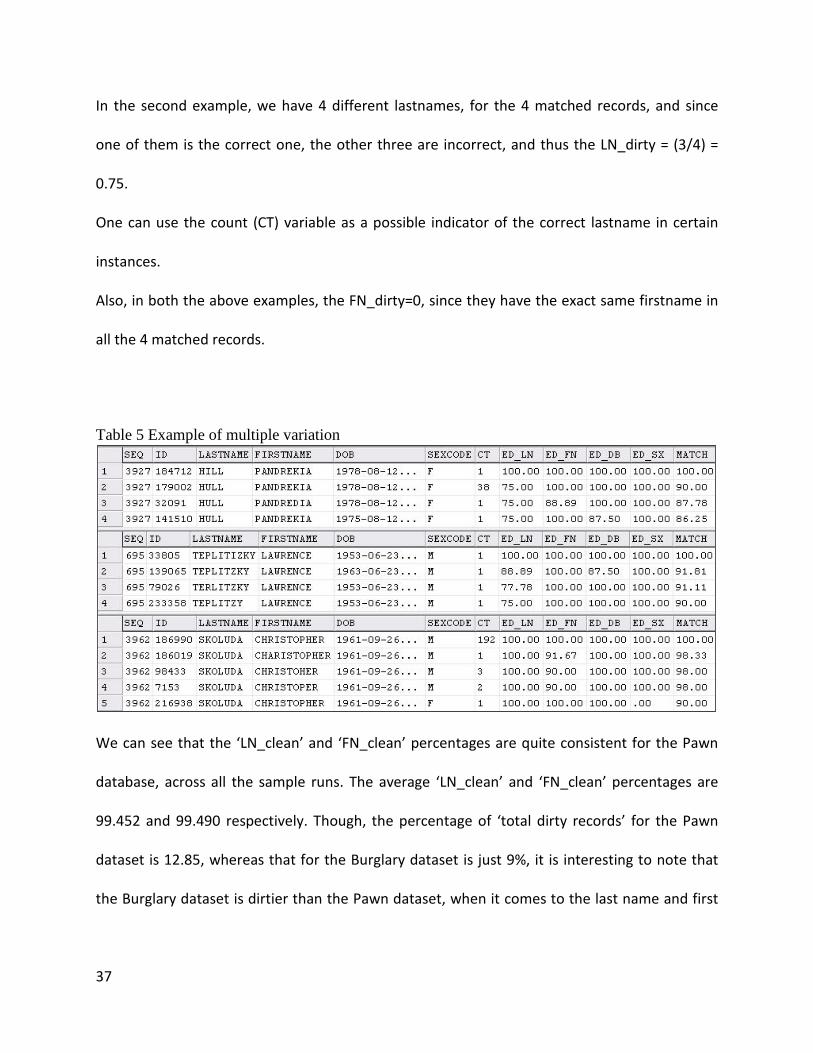
In the second example, we have 4 different lastnames, for the 4 matched records, and since

one of them is the correct one, the other three are incorrect, and thus the LN_dirty = (3/4) =

0.75.

One can use the count (CT) variable as a possible indicator of the correct lastname in certain

instances.

Also, in both the above examples, the FN_dirty=0, since they have the exact same firstname in

all the 4 matched records.

Table 5 Example of multiple variation

We can see that the ‘LN_clean’ and ‘FN_clean’ percentages are quite consistent for the Pawn

database, across all the sample runs. The average ‘LN_clean’ and ‘FN_clean’ percentages are

99.452 and 99.490 respectively. Though, the percentage of ‘total dirty records’ for the Pawn

dataset is 12.85, whereas that for the Burglary dataset is just 9%, it is interesting to note that

the Burglary dataset is dirtier than the Pawn dataset, when it comes to the last name and first

38

name variations for each person in the sample, as can be seen by the ‘LN_clean’ and ‘FN_clean’

percentages, which average 97.118 and 97.527 respectively.

The above is an example of measuring the data quality, when it comes to ‘record-level

uniqueness’, since we go through each record, which represents an individual, and then identify

the last name and first name variations for that individual, thus arriving at the cleanliness for

each record and further averaging it for the database.

We can also measure the data quality field-wise, thus arriving at the field-level uniqueness.

Thus, for the last name, we could arrive at the field-level uniqueness percentage for the last

name field, simply by calculating the number of last names which were dirty, divided by the

total number of last names in our database.

Following is the tabular summary of the sample runs on the Person table in the DSC database,

as also the Burglary dataset:

Run id Sample

size Last name cleanliness

First name cleanliness

No of dirty records

Pawn:

A1 1000 99.55 99.57 69

B1 1000 99.45 99.57 84

C1 1000 99.43 99.54 76

D1 1000 99.70 99.59 67

E1 4500 99.47 99.33 364

F1 1000 99.37 99.60 66

G1 1000 99.25 99.33 91

H1 5000 99.35 99.49 395

I1 5000 99.50 99.39 384

Burglary:

X1 4607 97.093 97.367 519

Y1 4611 97.143 97.687 499

39

Conclusion & Future Work

The literature review and the documentation studied on data quality clearly states the strong

need for having a tangible measure of data quality, since one cannot aim to have a very high

data quality without knowing how dirty the data is and the nature of the dirtiness. The

proposed Data-Cleanliness algorithm demonstrates how one can arrive at the dirtiness measure

of any database, which not only helps in setting up guidelines for the data clean-up process, but

also helps in comparing dirtiness measures across different datasets.

The algorithm can be further extended by arriving at cleanliness rules for other fields or tables

(for instance, one can compare DOB with AGE, if two such separate fields exist, and check to

see if they match, which they should.)

The future work can also include analyses on the dirtiness results, within the database, in terms

of a breakdown of the distinct types of dirtiness, which could further help us in understanding

the nature of dirty data. Each of these distinct types of dirty data can be associated with a

critical dirtiness number, say (based on the severity of the problems it can cause), which would

help us in prioritizing the data clean-up process, as also in cross-comparing various datasets not

only on the total dirtiness, but also the nature of dirtiness.

40

Data Validation of a Vehicle Identification Number (VIN) Dataset

Data input validation is a critical component of maintaining data quality in software systems. It

is important to avoid inaccurate data entering the system early in the data life cycle, as the cost

and effort in maintaining data cleanliness significantly increase over time. Data validation can

be handled either at the client-side or server-side or both, depending upon the type of

application, time for validation, bandwidth issues, type and sensitivity of data, security

requirements. Some of the common technologies used for data validation are regular

expressions, xml, and procedural code.

Regular Expressions: They are extremely powerful, consistent and a fast means of processing

textual information. They were derived in the 1940's while modeling neural functions as regular

sets, and further expressed as 'regular expressions'. These initially found their way into Unix

utilities such as 'grep' and are now supported extensively in different languages and platforms

(Forta, 2004). Regular expressions are one of the most efficient and simplistic means of data

validation.

XML: XML originated primarily as a means of representing data, allowing for a strong flexibility

in structuring data and further making data easily readable by any application on any platform.

XML schemas or XSD’s define the structure of an XML document, and thus, any XML data can

be strictly validated against its XSD. XML data validation also handles enumerations, which is

quite often a requirement for validating certain types of data.

41

Regular Expressions & XML: XML-based systems often harness the power of regular expressions

for pattern matching, and use XML schemas for data validation (Hosoya & Pierce, 2003).

Regular expressions have also been used as a means for inferring a schema for an XML

document when no valid one is present (Bex et al., 2008).

Procedural Code: Although procedural code offers all capabilities towards the application of

business rules for the purposes of data validation, it is not the most elegant means of doing so,

since it is cumbersome, and neither efficient nor manageable. “Validation scripts are even more

time-consuming and difficult to write than regexps, even for professional programmers”

(Scaffidi et al., 2008).

The Need for Data Validation

Our specific need is to validate data input that follows complex rules requiring both

enumerations and conditional decisions based on the enumerations. An example data type is

the VIN dataset.

The VIN or the ‘Vehicle Identification Number’ is a 17-digit number assigned to an individual

vehicle by the manufacturer, such that it contains all alpha-numeric characters and the VINs of

any two vehicles manufactured within a 30-year period shall not be identical.

42

The VIN dataset, because of the nature of its complexity, was specifically chosen for purposes

of data validation as against datasets pertaining to Social Security Numbers, Zip codes, IP

numbers, IDs, Credit card numbers, etc. to name a few. The VIN dataset is a complex one, since

the VIN number is governed by business rules, requiring it to satisfy both conditionals as well as

enumerations for its validation. The rules depend on a multitude of factors such as the

manufacturer, the country of manufacture, the vehicle make, the vehicle model, and so on.

There are different rules for different digit positions in a VIN.

Another characteristic of the VIN dataset when it comes to validation is that a single VIN can be

validated against fixed business rules.

Here is an example of a VIN for a vehicle manufactured by Ford:

‘1ZVHT85H695116999’

Position 1-3: WMI or the World Manufacturer Index

1ZV: Vehicle Manufacturer: Automotive Alliance International (USA)

Vehicle Make: Ford

Vehicle Type: Passenger Car

Position 4: Restraint System Type

H: Driver and Passenger Side Air Bags, Curtains or Canopies

Position 5-7: Line, Series, Body Type

43

T85: Car Line: Mustang

Car Series: GT

Body Type: 2-Dr. Convertible

Position 8: Engine Type

H: Displacement/Litre: 4.6L 3V

Cylinders: V-8

Fuel: Gasoline

Manufacturer: Ford

Net Brake HP: 300

Position 9: Check Digit

6: Valid Check Digit – must be between 0,1,2,3,4,5,6,7,8,9 or X.

Position 10: Model Year

9: Manufactured in 2009

Position 11: Assembly Plant

5: Vehicle Assembly Plant Location: AAI: Flat Rock, Michigan

Position 12-17: Production Sequence Number

44

116999: Valid Production sequence number – falls between 100001 thru 599999- Ford

Division Vehicles

Overview of Regular Expressions

Regular expressions are largely used for matching patterns in text, and also for validating user

input. Some of the diverse applications where regular expressions have been used are

sequential pattern mining (Garofalakis et al., 1999), deep packet inspection (Yu et al., 2006),

web search engines, lexical analysis, data validation such as emails/phone numbers/credit

cards/UPS tracking numbers etc., constraining user-input, extracting text from HTML, parsing

text and replacing values for data cleanliness, among many others (Bex et al., 2008, Lowe, n.d.,

Maddock, 2001, Dehaan, n.d., Meier et al., 2005).

The ability to use regular expressions realizing their potential, has been implemented by many

software companies such as Oracle in their 10g database (Linsley & Trute, n.d.), in Java (Shah,

2003), in SAS (Tabladillo, 2005) & also in (Mac users) Cocoa (Davis, 2003), to name a few.

Languages such as Awk, Elisp, Expect, Perl, Python and Tcl have regular-expression support built

in, since regular expressions are at the very heart of many programs written in these languages

(Friedl, 1997).

Although the basic regular expression syntax is for the most part, consistent among different

implementations, the way regular expressions are used is most definitely not; the languages

45

and applications that support regular expressions have their own subtle differences and

nuances (Forta, 2004).

Being extremely powerful, efficient and fast at processing text, our goal for this paper is to

explore the sole use of regular expressions and devise a framework for validating the VIN

dataset.

Our Approach

The VIN dataset has a lot of business rules to be validated against, especially conditional rules

and checks against enumerations. An example of such a complex rule is – If the 10th digit of a

VIN is 9, implying that the year of manufacture is 2009, then check whether the first 3 digits

(comprising the ‘World Manufacturer Index’ or WMI) of the VIN fall in a specified enumeration

(set of valid WMIs specified by a manufacturer for 2009), else check if the 10th digit is 8, and

check for a further set of rules, etc.

We decided to implement regular expressions in the .Net environment, for purposes of

validating the VIN dataset. Regular expression support in.Net is provided by the ‘Regex’ class

and other supporting classes, which offer various methods such as ‘IsMatch ()’, ‘Replace ()’, etc.

to manipulate text.

For any custom field to be validated, a ‘RegularExpressionValidator’ control is used to verify the

input. Each validator control translates to a given business rule and one can have as many such

46

controls as the number of business rules governing the VIN. However, this is not an elegant

approach, especially when one has a lot of business rules, as in our case.

We therefore propose encapsulating all the business rules governing VINs as regular

expressions and storing them in a database. At run-time, each of these regular expressions

representing a unique business rule gets assigned as an expression of the Validator control, and

all the validator controls together work towards validating the VIN. This not only provides a

strong business logic framework for VIN validation, but is also scalable and manageable since

any time the VIN rules have to be modified or any new rules have to be added, all that needs to

be done is to update the regular expression database and the assign the new rule-based regular

expressions to their corresponding validator controls.

Following is a table of some of the regular expression rules for the VIN dataset:

Table 6 Database table showing Regular Expression rules and their descriptions

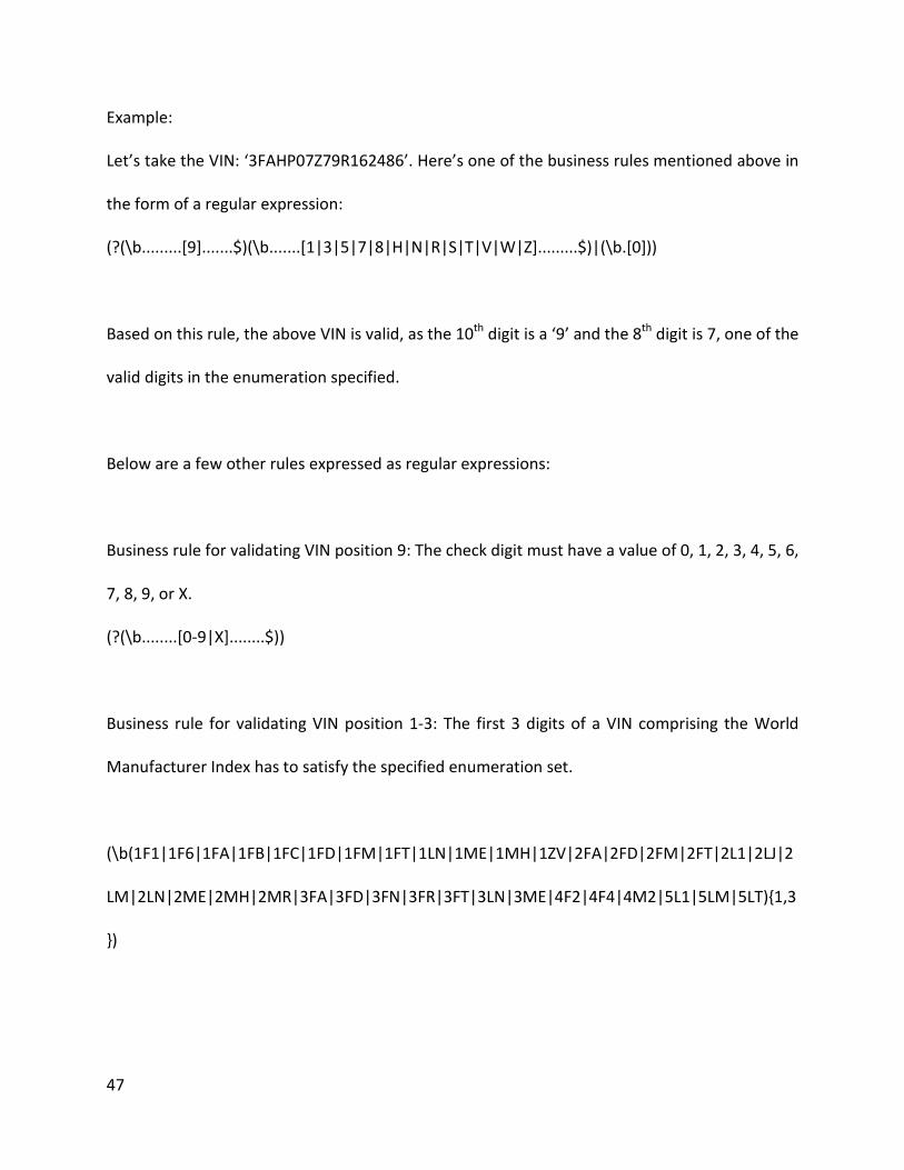
47

Example:

Let’s take the VIN: ‘3FAHP07Z79R162486’. Here’s one of the business rules mentioned above in

the form of a regular expression:

(?(\b.........[9].......$)(\b.......[1|3|5|7|8|H|N|R|S|T|V|W|Z].........$)|(\b.[0]))

Based on this rule, the above VIN is valid, as the 10th digit is a ‘9’ and the 8th digit is 7, one of the

valid digits in the enumeration specified.

Below are a few other rules expressed as regular expressions:

Business rule for validating VIN position 9: The check digit must have a value of 0, 1, 2, 3, 4, 5, 6,

7, 8, 9, or X.

(?(\b........[0-9|X]........$))

Business rule for validating VIN position 1-3: The first 3 digits of a VIN comprising the World

Manufacturer Index has to satisfy the specified enumeration set.

(\b(1F1|1F6|1FA|1FB|1FC|1FD|1FM|1FT|1LN|1ME|1MH|1ZV|2FA|2FD|2FM|2FT|2L1|2LJ|2

LM|2LN|2ME|2MH|2MR|3FA|3FD|3FN|3FR|3FT|3LN|3ME|4F2|4F4|4M2|5L1|5LM|5LT){1,3

})

48

Following is a screen capture of the webpage, highlighting the errors if any, during data

validation:

Figure 2 Data Validation implementation using Regular Expression Validators, highlighting any data errors

Conclusions

By taking the Vehicle Identification Numbers or VINs as an example, we provide a flexible and

scalable business logic framework for validating such a complex dataset against a specified

ruleset. The framework encapsulates the numerous business rules in the form of regular

expressions, which are stored in a database. Being generic, it can be successfully extended to

49

data such as driver’s license numbers, insurance id numbers, etc., where input validation can be

carried out on a single-field, without considering any other related data fields.

Future work for the proposed framework could include arriving at the extent of invalid data or

percentage mismatch, prioritizing data cleaning based on the severity of mismatch, identifying

probable reasons for invalidation, and the scope for correcting it. The robustness of such a

framework could be further improved by incorporating cross-validation across other data fields,

and exploring functional dependencies among key fields.

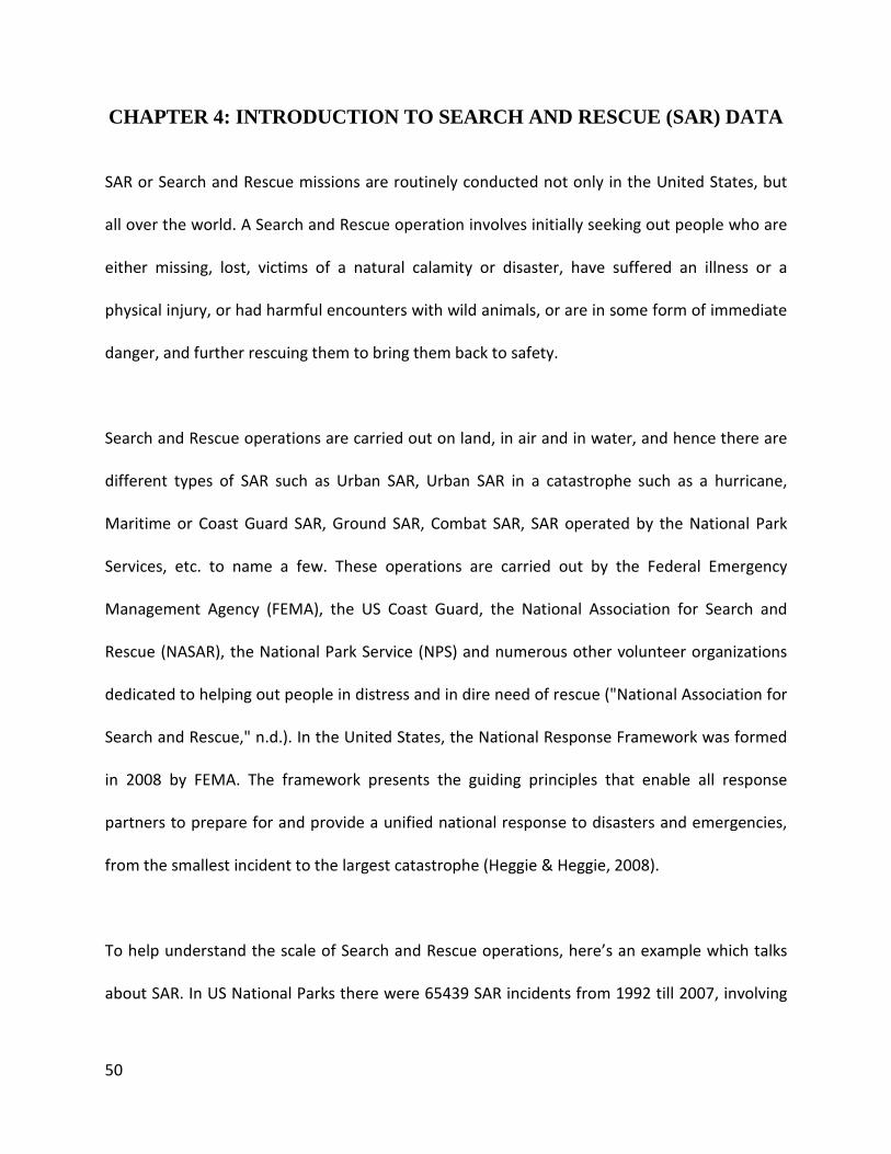
50

CHAPTER 4: INTRODUCTION TO SEARCH AND RESCUE (SAR) DATA

SAR or Search and Rescue missions are routinely conducted not only in the United States, but

all over the world. A Search and Rescue operation involves initially seeking out people who are

either missing, lost, victims of a natural calamity or disaster, have suffered an illness or a

physical injury, or had harmful encounters with wild animals, or are in some form of immediate

danger, and further rescuing them to bring them back to safety.

Search and Rescue operations are carried out on land, in air and in water, and hence there are

different types of SAR such as Urban SAR, Urban SAR in a catastrophe such as a hurricane,

Maritime or Coast Guard SAR, Ground SAR, Combat SAR, SAR operated by the National Park

Services, etc. to name a few. These operations are carried out by the Federal Emergency

Management Agency (FEMA), the US Coast Guard, the National Association for Search and

Rescue (NASAR), the National Park Service (NPS) and numerous other volunteer organizations

dedicated to helping out people in distress and in dire need of rescue ("National Association for

Search and Rescue," n.d.). In the United States, the National Response Framework was formed

in 2008 by FEMA. The framework presents the guiding principles that enable all response

partners to prepare for and provide a unified national response to disasters and emergencies,

from the smallest incident to the largest catastrophe (Heggie & Heggie, 2008).

To help understand the scale of Search and Rescue operations, here’s an example which talks

about SAR. In US National Parks there were 65439 SAR incidents from 1992 till 2007, involving

51

78488 individuals. Thus, there were 11.2 SAR incidents each day at an average cost of $895 per

operation, amounting to around $10000 per day (Heggie & Amundson, 2009).

Figure 3 SAR Operations by Year

The above graph shows the number of SAR operations carried out every year in the US National

Parks (Shafer, 2010). It can be seen that the SAR operations in the last 4 years from 2006 till

2009 seem to be steady and actually have averaged around 3572 operations every year.

Also, some of the interesting and noteworthy facts as cited by the article on Search and Rescue

in the National Parks (Heggie & Amundson, 2009) are:

In 2005 alone, more than 50% of the SAR operations occurred in just 5 NPS Units.

Yosemite National Park accounted for 25% of the total NPS SAR costs ($1.2 million).

52

Hiking (48%) and boating (21%) were the most common activities requiring SAR

assistance.

Hiking (22.8%), suicides (12.1%), swimming (10.1%), and boating (10.1%) activities were

the most common activities resulting in fatalities.

Without the presence of NPS personnel responding to SAR incidents, 1 in 5 (20%) of

those requesting SAR assistance would be a fatality.

As can be seen, SAR missions are extremely important to avoid any fatalities, and some critical

information can be gleaned through historically collected SAR data. Below is a snapshot of the

NPS SAR data from 2000 till 2007, which reflects that although the SAR missions carried out are

steady in the last 4-5 years, the SAR costs are definitely on a steady rise:

Table 7 SAR Statistics highlighting the rising costs of SAR Operations Year Total SAR

cost

Total SAR

Operations

Fatalities Illness or

Injured

Nonillness

or Injured

Save

2007 $4 735 424 3593 136 1218 2566 1023

2006 $4 524 875 3623 119 1445 2900 1211

2005 $4 996 705 2430 152 1129 2016 402

2004 $3 592 218 3216 127 1087 3077 815

2003 $3 468 255 3108 124 1199 2162 427

2002 $3 040 020 4537 129 1338 3492 1832

2001 $3 683 086 3619 123 1502 2782 155

2000 $2 779 967 4869 244 1471 3495 709

… …

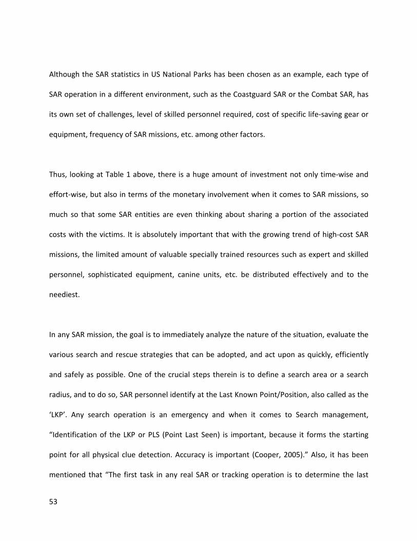
53

Although the SAR statistics in US National Parks has been chosen as an example, each type of

SAR operation in a different environment, such as the Coastguard SAR or the Combat SAR, has

its own set of challenges, level of skilled personnel required, cost of specific life-saving gear or

equipment, frequency of SAR missions, etc. among other factors.

Thus, looking at Table 1 above, there is a huge amount of investment not only time-wise and

effort-wise, but also in terms of the monetary involvement when it comes to SAR missions, so

much so that some SAR entities are even thinking about sharing a portion of the associated

costs with the victims. It is absolutely important that with the growing trend of high-cost SAR

missions, the limited amount of valuable specially trained resources such as expert and skilled

personnel, sophisticated equipment, canine units, etc. be distributed effectively and to the

neediest.

In any SAR mission, the goal is to immediately analyze the nature of the situation, evaluate the

various search and rescue strategies that can be adopted, and act upon as quickly, efficiently

and safely as possible. One of the crucial steps therein is to define a search area or a search

radius, and to do so, SAR personnel identify at the Last Known Point/Position, also called as the

‘LKP’. Any search operation is an emergency and when it comes to Search management,

“Identification of the LKP or PLS (Point Last Seen) is important, because it forms the starting

point for all physical clue detection. Accuracy is important (Cooper, 2005).” Also, it has been

mentioned that “The first task in any real SAR or tracking operation is to determine the last

54

known position (LKP). For SAR, this is a critical step, since the accuracy of this information is

decisive for the outcome of the search” (Hackett et al., n.d.). The author describes a scenario

where say, if a distress call is received from a ship with a GPS unit, if the LKP is precisely known,

then a small radius of search with all candidate members being released at the same point is

possible. However, if little is known about the time or the incident location, a wide radius and a

long period of time must be used.

The LKP clearly forms the basis of the type of search strategy to be used, the search perimeter,

the effective area of sweep, etc. among many other factors. Each organization conducting the

SAR has its own way of documenting data related to SAR, and many a time, the LKP data is

missing or non-existent.

Also, at times, the LKP is specified in a vague manner, i.e. a 'trailhead' or 'near I-70 (Interstate

70) 200 mm (mile marker)', etc. and it becomes critical that this LKP data be translated to a pin-

point location on the map, which is essentially the process of 'geocoding'. There are numerous

other benefits of geocoding the LKP, which are discussed later.

The goal of this research as applied to the SAR dataset is to improve the accuracy of the LKP

data wherever possible, with a view to fully geocoding it, so that one is able to visualize and

plot the LKP on a map, for further analysis.

One of the challenges with regards to the SAR data being worked on is that the collection

process is not perfect. Often, the LKP is not known or cannot be arrived at. A very small

55

percentage of the LKP coordinate data (7 %) is populated, and also, in the data that is

populated, the coordinates aren’t given as “coordinates” sometimes. As stated in the article

regarding SAR in the Yosemite National Park, a 10-year review (Hung & Townes, 2007),

‘Notification of Yosemite National Park authorities of an incident needing SAR services occurred

by radio or standard telephone (61%), verbal communication (34%) or cellular phone (5 %)’.

Thus, it is understandable that when park officials get to know about a SAR mission, it is almost

always through some type of verbal communication, and hence the documentation of the SAR

data is not always clear or complete. Also, the mode of communication allows for a possibility

of human errors creeping into the dataset, especially when it comes to coordinate details or

important numeric data.

Geocoding

Geocoding is simply the process of mapping the address information. An address includes any

type of information that distinguishes a place. The process of geocoding, or assigning a location

in the form of coordinate values to an address, is carried out by comparing the descriptive

location elements in the address to those present in the reference material (Crosier, 2004).

Thus, geocoding involves translating the street, city, zip code and any other address

information into geographical coordinates, thereby enabling the user to arrive at a specific

point location on a map. For instance, if an address, say ‘Excelsior Reserve, Larra Cres, Nth

Rocks, NSW, Australia’ can be converted in coordinate form, ‘315150/6252666 (where ‘315150’

56

is the Northing coordinate and ‘6252666’ is the Easting coordinate)’ as in this case, and can be

further accurately plotted on a map, then we have successfully geocoded the address.

Different levels of Geocoding

There are various levels of geocoding the address information, and this is referred to as ‘Partial

address geocoding’. The process of geocoding can be carried out through different types of

software or geocoding services. One of the most common methods employed to geocode

address information is using the ArcGIS or ArcMAP services provided by ESRI, the pioneer in GIS

(Geographical Information Systems) services. Other geocoding software are Oracle 10g’s Spatial

Suite, Microsoft Bing Services or any other third party address geocoding services.

Depending on the specific software used for geocoding, one can achieve different levels of

partial address geocoding such as House-level, Intersection-level, Street-level or Place-level

geocoding. As the type or level of geocoding implies, house-level geocoding simply means that

the address can be geocoded at a house-level, i.e. the house can be pinpoint located on a map.

The same holds true for intersection, street and place-level, where based on the information

available, an intersection, a street or a place can be successfully geocoded. A place could be a

geographical region with boundaries, in which case, it can be represented as a polygon plotted

on a map. A place such as a city or town could also be represented by highlighting or displaying

a point, which is the centroid of that city or town. The levels of partial address geocoding vary

based on the geocoding software used.

57

There are several reasons as to why some addresses can only be partially geocoded. Mostly,

this is because of incomplete or missing information provided in the address fields. For

instance, if a street suffix is missing and if there exist two streets by the same name in a

particular city, or across states, the geocoding software can only geocode it accurately at say,

the city level or then the state level. Another reason is that the address information although

complete, may not be accurate and hence the software used for geocoding may not be able to

assign coordinates to that particular address, and hence partial geocoding is the only solution.

For example – if for a valid city, zip code and state, the street specified in the address

information cannot be matched with the geocoding software address reference, then the best

possible way to geocode is partial geocoding at the city-level, assuming that the city has been

correctly entered when the address information was captured.

The Google Geocoding API

The Google Geocoding API (The Google Geocoding API, n.d.), an open-source means of

geocoding addresses, was selected to be the geocoding software used for geocoding the LKP in

the SAR dataset. The API is quite easy to use, has a lot of built-in features and is considered

fairly reliable and suitable for our purpose, especially with Google’s reputation for advanced

and innovative technology-driven services. Also, the Google API allows for geocoding of

addresses all over the world.

In our dataset, the goal of geocoding is to arrive at the pinpoint location of the LKP on the map,

based on as much address information as can be gathered, either provided in the address-

58

related fields or then through extraction from other non-address related fields in the dataset.

The Google geocoding API does allow for partial-level geocoding, and includes the level of

geocoding as a part of the query response in the ‘geometry’ field. Whenever an address is sent

to the Google API, the geocoder includes in the ‘geometry’ field, both the location details as

well as the ‘location_type’ which is an indicator of the level of geocoding, either precise or at

different levels of partial geocoding. This allows us to use partial-level geocoding as an option,

where fully geocoding the LKP is not possible on account of incomplete information.

Thus, our focus is to fully geocode the LKP, for as many data points as possible, partially

geocoding the rest of the data points wherever possible and to further identify those data

points where the LKP cannot be fully geocoded.

Geocoding as applied to the SAR dataset

As mentioned earlier, the LKP is one of the most important factors in any search and rescue

mission. Geocoding the LKP and plotting the LKP on a map would lead to determining the

search strategy and the effective area of sweep (Cooper, 2005). It would also help organize and

better the search process, by taking into account the terrain conditions, any nearby land

markers and other geographical factors, which can be analyzed only if the LKP has been

geocoded.

Also sometimes in rural areas, geocoding layers are unavailable or not as well developed

(Dramowicz, 2004). It is quite possible that in some state parks or national parks, if the LKP

59

coordinate points cannot be arrived at, the search strategy might not be effective or the search

process would take a lot of time.

Plotting the LKP on a map may help discover some patterns evident only through visualizing the

geocoded LKP data. For instance, say after visualization, it is revealed that a majority or 80% of

the victims get lost in a specific area of the park, or on a particular trail in a most commonly

frequented state park. This certainly indicates a pattern, and would in-turn prompt some more

safety features or steps taken in that park to avoid hikers getting lost or injured, etc., which is a

proactive action on the side of the park officials to reduce the SAR missions in the park, as also

conserve SAR resources.

Finally, geocoding would help as a great input to data visualization and thus data

summarization. It would help achieve a good understanding of the SAR incidents, as one can

highlight the successful ones or the most expensive ones, and thus would undoubtedly prove to

be a very useful tool.

The GNIS Database

The Geographic Names Information System (GNIS) database contains information about

physical and cultural geographic features in the United States and associated areas. The GNIS

was developed by the U.S. Geological Survey (USGS) in cooperation with the U.S. Board on

Geographic Names (BGN), to promote the standardization of feature names.

60

The database holds the Federally recognized name for each feature and defines the location of

the feature by state, county, USGS topographic map, and geographic coordinates. The GNIS

data contains feature names and the corresponding feature classes for each state in the United

States, and has more than two million records. Some of the attributes include names or

spellings other than the official name, feature designations, historical and descriptive

information. The database assigns a unique feature identifier, a sequential number, which is a

key for accessing, integrating, or reconciling GNIS data with other datasets. The GNIS is the

Nation's official repository of domestic geographic feature names information (Heggie &

Heggie, 2009).

Below is a snapshot of the GNIS database containing feature names for the state of Florida:

Table 8 Sample records for the GNIS Database

61

For instance, in the above table, in one of the records (feature_id=277631), the feature_name

‘Chuluota’ is a city name, since its feature_class is a ‘Populated Place’. One of the other feature

names (feature_id=277632) is a state park, namely the ‘Collier-Seminole State Park’, since its

feature_class is a ‘Park’.

The use of the GNIS dataset in the SAR Algorithm shall be discussed in detail in the subsequent

chapter.

The SAR Dataset

The Search and Rescue (SAR) data has been aggregated from incidents all across the world.

Majority of the data points (around 80 %) are from the United States, spread across several

states, while the rest of the data is split among Australia, Canada, New Zealand, UK and South

Africa.

The SAR data spans around 70 columns or variables, capturing specific SAR operation

information such as the incident details, the terrain, the weather conditions, the number of

people involved, the activity of subjects, their physical details, the location details, the effort in

terms of total man hours and total dog hours, the rescue method, the geographic details of the

area where the subject/s were found and finally the comments, which include additional

information about the SAR incident, which cannot be entered in the defined fields.

The dataset has about 30,000 records, and our goal for this dataset is to identify the percentage

of data points which can be geocoded fully given the address-related information in the address

62

fields, geocoded partially based on the available incomplete information, but which can be

supplemented using other data fields and those which cannot be geocoded at all. Ideally, the

higher the number of data points which can be geocoded, the better it is.

Here's what the SAR data looks like, through a couple of data points taken as examples:

63

Table 9 Sample records for the SAR Dataset columns 1 through 8

Table 10 Sample records for the SAR Dataset columns 9 through 15

Table 11 Sample records for the SAR Dataset columns 16 through 25

Table 12 Sample records for the SAR Dataset columns 26 through 34

Table 13 Sample records for the SAR Dataset columns 35 through 39

Table 14 Sample records for the SAR Dataset columns 40 through 49

Table 15 Sample records for the SAR Dataset columns 50 through 57

64

Table 16 Sample records for the SAR Dataset columns 58 through 63

Table 17 Sample records for the SAR Dataset columns 64 through 70

Table 18 Sample records for the SAR Dataset columns 71 through 77

Table 19 Sample records for the SAR Dataset column 78

The following columns in the dataset are regarded as the most helpful for plotting the LKP,

since they contain the geographical address information needed for geocoding the LKP:

‘Data Source’ – The source of the data record, which contains the country of the SAR incident,

and also the state, if the country is the United States

‘LKP Coord (N/S)’ – The Northing coordinate specified for the Last Known Position or the LKP

‘LKP Coord (E/W)’ – The Easting coordinate specified for the Last Known Position or the LKP

‘City’ – The city of occurrence for the SAR incident

‘County’ – The county of occurrence for the SAR incident

‘Comments’ – The narrative comments pertaining to the SAR incident

65

‘LKP Type’ – The type of Last Known Position, or some additional information about the SAR

incident in some cases

Here is some sample data contained in the above-listed important columns in the SAR dataset:

Table 20 SAR Data subset containing fields important for geocoding

Here are some more column-specific examples:

Different representations of the geographical coordinates, in the ‘LKP N/S’ fields/columns:

Table 21 Examples of variations in coordinate formats for Australia

Table 22 Examples of variations in coordinate formats for Canada

66

Table 23 Examples of variations in coordinate formats for New Zealand

Table 24 Examples of variations in coordinate formats for Arizona, US

Table 25 Examples of variations in coordinate formats for New Jersey and New York, US

Table 26 Examples of variations in coordinate formats for New York, US

67

Table 27 Variation in coordinate formats across the US state of Washington

Data representing the last known position, in the ‘LKP Type’ field:

Table 28 SAR Data subset highlighting the [LKP Type] field

68

The ‘LKP Type’ field is supposed to specify the type of the last known position, say a ‘trailhead’,

a ‘street’ or say, an ‘interstate highway’. As seen from the table above, which highlights some

examples of the text in the ‘LKP Type’ field, it does contain some address-related information

such as proper nouns or street names, and feature names, and hence it is worth extracting any

relevant information from this field, in case the other fields do not carry sufficient address

information.

Table 29 Data in the 'comments' field

The ‘Comments’ field contains all the unstructured text, which is nothing but additional

information about the SAR incident. It does contain several specifics embedded in the text, for

e.g. - information about the age of the Missing Person (MP), some relevant dates, time of

occurrence, street-specific information such as the street name, or the street number or the

city/county name, some landmark or a feature name, and at times even the LKP coordinates.

For instance, the first record (key#=AU-0041) in Table 23 above, the ‘Comments’ field has the

UTM coordinates specified. Also, in the records (key#=AU-0426, and key#=UC-CO1182) there

are street names specified – ‘Gunrock Fall Fire Trail’ and ‘Hessie Trail’ respectively. And in the

record (key#=NZ-1503), a feature name – ‘Rimutaka Forest Park’ has been mentioned. Such

69

information in the ‘Comments’ field would be worth extracting where the data in the address

fields is insufficient for either fully or partially geocoding the LKP.

70

CHAPTER 5: SAR ALGORITHM – APPROACH, ANALYSIS & RESULTS

Search and Rescue (SAR) operations carried all over the world by different governing

organizations require a wealth of expertise, meticulous planning, and a dedicated task force

specially trained and equipped for seeking victims, which are faced with some form of danger

and rescuing them to safety. The details of such SAR operations are studied and the data is

typically analyzed at various levels. Some of the key purposes for analysis are to reduce costs or

identify areas where the costs can be reduced, to allocate SAR resources to the most critical

operations in such a way that the distribution of resources is optimal, to gain a strong insight

into identifying search strategies for future SAR operations based on past data, to seek ways in

which the number of such incidents can be reduced and the general public can be educated or

made aware of the risks in certain areas, etc. One of the research areas being conducted on SAR

data is to build/generate probability maps to help predict location of the victims, for similar

situations based on historic data ("Bayesian Models for Search and Rescue,"n.d.).

The SAR data has numerous quality issues. Data for many fields is not populated and hence the

data is incomplete. Also, the data formats are quite inconsistent, and there’s a lot of variation in

the formats specified. Some of the data is not valid, and a lot of useful data resides as

unstructured text. Essentially, the SAR data has numerous instances of different types of

dirty/bad data. The goal for this study/research with regards to the SAR dataset is to apply

methodologies and techniques for cleaning the data with a view to geocoding the LKP. An

algorithm has been developed which focuses on cleaning and validating some of the data fields,

identifying the address-related information, extracting it from the various fields and then

71

geocoding the LKP based on the extracted information. Thus, the SAR Algorithm shall geocode

the LKP, fully or partially, for as many data points as possible, and shall arrive at the percentage

of records which are unable to be geocoded, also in turn highlighting the reasons for the same.

As mentioned in the previous chapter, the most important fields in the SAR data for the

purposes of geocoding the LKP have been identified, namely the Data Source, City, County, LKP

coordinate (N/S), LKP Coordinate (E/W), Comments and LKP Type, and the SAR Algorithm relies

on some or all of these fields for geocoding the LKP, based on the information available in these

fields.

After analyzing the above described fields, and identifying all the address information

contained therein, the relevant information is aggregated into an ‘address string’ and

subsequently passed to the Google Geocoding API. Whenever there is a match found, the

Google API successfully geocodes the address, and gives us the location coordinates of the

match. Sometimes the Google API finds multiple matches, based on the address strings passed

for a single record, and hence outputs multiple coordinates, which are also captured in the

database. These coordinates can further be plotted on a map, and could also be verified visually

against the city, county or then the state information. Any discrepancy, if at all, implies a

limitation of the Google API, or then hints at a possibility of underlying erroneous data and is

thus an indication of the quality of the geocoding software itself. It could also be the very

infrequent case of two different states say, having the same street names and street numbers,

and such records can further be manually verified.

72

The Google API outputs the coordinates in a specific coordinate system format, and in order to

maintain consistency for a particular nation or state, we shall be using the Google API output

format for geocoding and plotting. Also, we can convert the coordinates in the SAR dataset

from the specified format to the one output by the Google API, using a third party online

coordinate format conversion system (“RCN Utilities & Tools,” n.d.), or by manual conversion

applying the known rules of conversion across various formats.

Following are the key analysis points to be focused on, with regards to the SAR algorithm:

When address fields have been populated

Of the fields identified as important in the SAR dataset, the following directly reflect the

geographical address information:

Data Source

City

County

The ‘Data Source’ field is a two character or sometimes a five character string, the first two

digits of which represent the country. Where the ‘Data Source’ string length is more than two

characters, typically, the first two digits represent the country, either the United States or

Canada, and then the last two digits, which are separated from the first two digits by a hyphen,

73

represent either one of the states in the US or then a province in Canada. This field has hardly

any values missing, and hence for purposes of analysis, the country is almost always specified.

The ‘City’ and the ‘County’ fields represent correspondingly the city and the county information

in the specified country. In this particular dataset, many a time, the ‘City’ field contains a street

address, a common land mark, or then some descriptive data about the place, Thus, the ‘City’

field either contains a city, or some feature name information related to the SAR incident, for

instance ‘Eaglesnest Wilderness’, ‘Molly Brown Campground’, ‘70km East of Normanton’, to

highlight a few. The ‘County’ field, when populated, does specify the county most of the time.

Out of the remaining fields, namely the LKP coordinate (N/S), LKP Coordinate (E/W), Comments

and LKP Type, since the two coordinate fields when populated can be readily used for

geocoding, the other key fields used for geocoding, are the ‘Comments’ and the ‘LKP Type’

fields. Both of these contain additional information about the SAR incident, especially the

‘Comments’ field, where the comments string at times contains city names, feature names, age

of the missing person, time of the day and such details.

Thus, all the relevant field-based address information is passed to the Google API, and

wherever there is a perfect match found, the Google API successfully geocodes the address,

and gives us the location coordinates of the place.

74

When address fields alone prove insufficient

It is quite possible that after sending the specific address information fields, the Google

Geocoding API is unable to fully or even partially geocode some of the passed data points. This

could be attributed to a number of reasons. The address information could be inaccurate,

incomplete or missing, and invalid. At times, the SAR incident location could represent a

geographical location which falls either in a rural area or in the remote wilderness, and for

which the geocoding reference layers may not be present. Hence, the Google API would be

unable to arrive at specific coordinates for such locations.

For those records, where the Google API is unable to fully geocode the address data, especially

in instances where the ‘City’ is missing, which leaves us with just the country, the state and the

county, additional identified fields in the data, namely the ‘Comments’ and the ‘LKP Type’ need

to be looked at, to check if any further address-related information about the incident can be

gleaned from the data. There are also several other fields in the dataset, such as the

geographical region or the ‘EcoRegion’, weather conditions, population density, etc. which

could perhaps add to the address information.

In case of any incomplete information, some techniques of imputing the missing data can be

considered by basing them on ‘similar’ other instances in the data. Also, data cleaning can be

carried out wherever possible, in order to correct any inaccurate or invalid information, before

the Google Geocoding API has been invoked.

75

All the above techniques can be implemented to arrive at any additional address-related

information, and if so, the address string to be passed, can be reformatted and resent to the

Google API, with a view to successfully geocoding the LKP for these data points. However, even

after sending all the address-related information associated with the SAR incident to the Google

API, if some records still come out with no coordinates specified by the Google API, these are

treated as ‘unable to be geocoded’.

Where the records are unable to be geocoded

Some of the main reasons as to why the data points cannot be geocoded are:

Insufficient address information to zero-in on the exact locational coordinates to enable

fully geocoding

Sufficient address information, however invalid data, and hence cannot be geocoded.

Sufficient address information, however non-matching with the Google Geocoding API

Reference Layers, because of –

Inaccurate information

Geographical constraint, for instance the location being in a rural area/wilderness area/

national park, and this could be a limitation of the geocoding software in terms of unable to

create reference layers for that location

The goal is to try and find the percentages of each category of data points where geocoding

cannot be carried out.

76

When LKP coordinates have been specified

In the SAR dataset, there are 2152 instances, which is 7% of the dataset, where both the LKP

coordinate fields, namely ‘LKP coord (n/s)’ and ‘LKP coord (e/w)’ are populated.

Geographical coordinate system formats vary from country to country, and there are different

ways of representing the exact location for any given place. Thus, some of the coordinates

cannot be successfully plotted on a map, the main reasons for which are:

Invalid coordinates, which means that they fall outside the permissible range of values

for a particular coordinate system and hence cannot be plotted or represented on a

map. This could be attributed to the following:

Small errors in specifying the number of digits or say, a shift of a decimal.

Incorrect data, say for instance the Northing coordinate is proper, however the Easting

coordinate has some error.

Valid coordinates, however not the proper coordinates for that location, thus implying

inaccurate or erroneous data. For instance, they could be coordinates for the previous

row, because of a shift in the data when aggregating all the data together and hence

indicates a need to check the data quality of the collection process, if such errors are

traced.

77

Valid coordinates, however when mapped, point to some other location, or simply

cannot be mapped, primarily since they are represented in a very unique and a

coordinate system format, which is unique to a specific geographical area such as New

Zealand, and uses a very specific datum, and also since the coordinates are inconsistent

between the northing and the easting coordinate.

Thus, not all of the 2152 coordinates’ populated data points can easily be geocoded to an actual

location. There are some online third party tools, which allow users to convert coordinate data

from one format to the other. Google’s Geocoding API gives us the coordinates in a degree

decimal format. However, a percentage of these 2152 instances is used to validate the SAR

Algorithm. The validation is carried out by initially removing both the populated coordinate

fields from the data, and using the SAR Algorithm on the rest of the important fields, namely

the Data Source, City, County, Comments, and LKP Type to obtain their coordinates from the

Google API. These obtained coordinates are then compared to the actual coordinates, by

converting between coordinate formats, if needed and thus the accuracy of the SAR Algorithm

can be arrived at. The details shall be discussed in the SAR Algorithm Validation section later on.

SAR Algorithm flowcharts

The SAR algorithm looks at each of the seven identified important fields for any address-related

information, and after doing so, determines the aggregated address information to be passed

to the Google API. The country, the state, the county and the city form the broad fields which

the algorithm looks at initially. Based on the information present in these fields, the algorithm

78

goes on to check the additional textual information in the other fields, extracts information

from them wherever possible and further determines the ‘address string’. However, when the

city and the county fields are either missing or do not have valid information, the algorithm

needs to look in the other fields to arrive either at say, the city, county, street details, feature

name, etc. present in the remaining textual fields. Thus, in case any of the important fields have

missing, incomplete or invalid data, there are different paths which can be traversed to obtain

the address information from other fields, and hence the SAR algorithm is well represented by

means of a flowchart.

79

Below is the overall main flowchart for the SAR Algorithm:

Figure 4 Flowchart for the SAR Algorithm

80

The flowchart comprises of three different types of shapes – rectangles, diamonds and ovals.

The rectangular shapes denote the important fields identified in the SAR dataset for purposes

of geocoding. The diamond shapes denote the conditions for the different fields, based on

which the path can be traversed. The oval shapes denote the end point for each path.

The flowchart has been numbered in small red-bordered boxes, so as to distinguish each and

every path. Each such red box has two numeric values either below it or on its side, which

denote the number of records for that point in the flowchart, and the percentage of the

occurrence of these records in the entire dataset respectively. For instance, the starting point

of the flowchart has been numbered as the red box marked as the Decision Point 1 [DP@1].

The first value below the box is specified as 30707, which is the number of records in the

dataset at that point, and since it is the starting point, 30707 is the total number of records we

have in the dataset, and hence the second value is 100 %. The number of records and the

corresponding percentages exist for the important pathways in the flowchart, especially the

starting paths. The flowchart starts from the top left corner and traverses downward and

sideways depending on the conditions satisfied.

The flowchart also contains some grey color coded small-sized boxes, which stand for detailed

flowcharts at that point. For instance, the first grey box marked as ‘D1’ at Decision Point 2

[DP@2] in the overall flowchart denotes a detailed flowchart which exists for ‘Plotting and

Validation’. All the detailed flowcharts are explained in the later sections.

81

To begin with, wherever the LKP coordinates have been specified, assuming that the

coordinates are valid, accurate and complete (both the coordinates have been specified), those

records do not have to be sent to the Google API for geocoding. Hence, the SAR Algorithm first

begins with the LKP coordinate fields and checks to see if they are populated. The following

flowchart component corresponds to the LKP coordinates:

Figure 5 Flowchart component for 'Plotting and Validation'

Starting at [DP@1] in the flowchart, the first branch is based on whether the LKP coordinates

are specified. If yes, the path branches to [DP@2] which has 3099 instances out of 30707,

roughly 10% of the data. [DP@2] further has a detailed flowchart for ‘Plotting and Validation’

which shall be discussed later. If none of the LKP coordinates are specified, the path branches

to [DP@3], which has 27608 instances. Thus, essentially 27608 records exist where the address

information has to be aggregated, based on the important fields identified and further passed

82

to the Google API. As mentioned earlier, the SAR Algorithm looks at the fields directly reflecting

the address. However ‘Data Source’ being populated for all the records, the country for each

record is given, and in case the country is ‘United States’, the state is also given for a majority of

the cases. Hence the subsequent branching in the overall flowchart starts with the ‘County’ and

the ‘City’ fields, in that order, since a county typically spans a larger geographical area than the

city.

Figure 6 Flowchart component for ‘County’

At [DP@3], if the County has been specified, the path branches to point [DP@4], and that holds

true for 25,340 instances. [DP@5] denotes those instances where the ‘County’ has not been

populated, i.e. 2268 instances. The next field to be checked is the ‘City’ and [DP@6] and

[DP@7] denote instances where the city specified is yes and no respectively. If none of the

‘County’ or the ‘City’ fields has been populated, the SAR Algorithm further looks at the

83

remaining fields, i.e. ‘Comments’ and ‘LKP Type’, so as to extract any relevant address-related

information from these fields. Thus, [DP@8] and [DP@10] in the flowchart represent the

scenario where comments have been inserted, and the LKP Type described. Similarly [DP@ 9]

and [DP@11] in the flowchart correspondingly denote the scenario where these two fields have

not been populated. To summarize, [DP@1] through [DP@11] represent the SAR Algorithm

looking at each of the fields in the order of importance for geocoding, with a view to aggregate

the address information and geocode the LKP wherever possible.

For each of the points in the flowchart, where these address fields have been populated, the

SAR Algorithm checks for clean data, takes steps to validate the data and looks at the other

fields to extract as much address-related information as possible. For instance, at points 4 and

6, which represent the ‘County’ and the ‘City’ fields being populated, the SAR algorithm checks

whether these are valid and then looks at the rest of the fields to combine any more

information if any, so as to be passed to the Google API.

84

Figure 7 Flowchart path 1-3-4-12-25-26-31

85

To take an example, path 1-3-4-12-25-26-31represents the flow in which the LKP coordinates

are not specified, the ‘County’ given has been validated, the ‘Comments’ have been inserted,

and the ‘LKP Type’ hasn’t been described. It is to be noted that although the ‘City’ field is being

checked at a later stage in the flowchart, the SAR Algorithm does check for each field before

finally forming an address string. To further explain this, in the above scenario, where a valid

county has been specified, to fully geocode the LKP, there is a higher priority associated to

check for any street addresses or any other address-related information such as feature names

embedded in the textual fields, as against checking if the ‘City’ field has also been populated.

However, if the textual fields do not yield any substantial address information, the ‘City’ and

the ‘County’ fields together will ensure a partial level geocoding of such records. Thus in the

above path, if the ‘City’ field exists, it would be considered for the formation of the address

string. The overall flowchart describes the prominent paths the SAR Algorithm takes in each

scenario, since it is not feasible to display the all possible paths in the main flowchart shown.

Another example is the path 1-3-4-7-8-16-20-33, which represents records where the ‘City’ and

the ‘County’ have not been specified, and just the ‘Comments’ field has been populated. As can

be seen, the percentage of such type of records is less than 1%, and the ability to geocode such

records depends on the nature of the comments inserted about the SAR incident, and whether

the address-related information in the ‘Comments’ field is sufficient for the purposes of

geocoding.

86

In the overall main flowchart, as can be seen, each flow reaches an end-point which is the

action to be taken at the end of that path. Thus, [DP@2] leads to an end-point which is ‘Plotting

and Validation’. Similarly, [DP@30], [DP@ 31], [DP@28], [DP@32], [DP@33] and [DP@22] lead

to all the aggregated address data passed to the Google API for geocoding. Finally, [DP@19]

reaches an end-point ‘Cannot be geocoded’, and also, [DP@23] reaches an end point ‘Extracted

information passed to a domain expert’.

87

Figure 8 Detailed Flowchart for 'Plotting and Validation'

88

As mentioned in the previous section, [DP@2] in the flowchart represents an end-point

‘Plotting and Validation’ which has been broken down into a detailed flowchart. Thus in the

above detailed flowchart ‘D1’, the starting point is [DP@2].

The branch to [DP@2] was based on the condition if the LKP coordinates were specified. The

3099 instances or 10% of the data, at this point represent those records where at least one of

the coordinate fields had been populated. The branching after [DP@2] leads into the break-

down of the coordinate fields. The LKP Northing coordinate has been specified for all of the

3099 instances as represented by [DP@200], and thus [DP@201] has 0 records. Similarly, out of

the 3099 instances at [DP@2], [DP@202] represents 2152 instances, where the LKP Easting

coordinate has been specified, and [DP@203] represents 947 instances where the LKP Easting

coordinate is not populated.

The flowchart is thus broken down into only the LKP Northing coordinate present, only the LKP

Easting coordinate present and both the LKP Northing and Easting coordinates present. 2152

instances or 7% of the entire data satisfies the last condition where both coordinate fields are

populated. At this point, the branch condition as to whether both the coordinate fields are

consistent leads to [DP@206] and [DP@207], where if they are consistent as in point 206, these

records can be plotted onto a map using the Google API. However if the two coordinate fields

are not consistent with each other, as represented by [DP@ 207], some consistency rules are

checked for, so as to identify where the inconsistencies lie.

89

Since there are no records where only the LKP Easting coordinate is present, the flowchart from

[DP@200] branches into [DP@204] and [DP@205], by checking for a scenario where the LKP

Easting coordinate has been included in the LKP Northing field, and this is based on some

checking rules which have been identified. If this is the case, as represented by [DP@204],

there is a data cleaning phase where the LKP Easting coordinate is separated from the LKP

Northing coordinate.

90

Figure 9 Detailed Flowchart for Invalid County

91

The above flowchart is a detailed flowchart for [DP@13] in the overall main flowchart, which

represents those records where the ‘County’ field has been populated, however the county

specified is invalid. The U.S. Geological Survey (USGS) as well as the U.S. Census Data provide

data for all the counties in a particular state, and thus the county data has been downloaded

from the above entities. The data provides the name of the county, its numeric identifier and

the name of the state in which it resides. This downloaded data is captured into a table against

which the counties present in the SAR dataset have been validated. For countries other than

the United States, say Canada or New Zealand, some research has been done to identify the

basic regions or provinces or territories based on the country and the tables for each country in

the SAR dataset have been populated to validate other counties or regions.

Figure 10 Examples of invalid counties in the SAR dataset

92

The above screen capture displays a few instances of invalid counties in the SAR dataset. As can

be seen in the flowchart, [DP@13] represents those instances where the ‘County’ field has

been invalidated and there exist 3168 such instances in the entire SAR dataset. From this point,

the flowchart branches into [DP@130] and [DP@131], based on whether the counties are

located in the US. At [DP@131], where the invalid counties are not in the US, a popular

algorithm for string matching, namely ‘Edit distance’ or ‘Levenshtein distance’ is used for

validating some of the counties (Levenshtein, 1966). An edit distance value of 2 has been used.

Thus if the actual county is ‘Brevard’, both ‘Breward’ and ‘Breword’ counties shall be treated as

valid counties. At point 138, where the edit distance is less than or equal to 2, such counties are

manually validated to avoid false positives creeping in. Thus, say for instance, if ‘Clay’ and ‘Bay’

are valid counties, a county spelt as ‘Blay’ and which is within an edit distance of 2 from each of

the two counties, cannot be confidently validated since it could be either of the two valid

counties. Thus [DP@140] represents instances where within the edit distance rule applied, the

county can be manually validated, and [DP@141] represents instances where the county

cannot be manually validated, and other ways are looked at to check if the county can be

validated.

Some other checks while validating the counties are done if the county is located in the US. The

counties in the US also have numeric identifiers, and hence wherever there are numeric

instances in the dataset for US counties, as represented by [DP@132], the numbers are checked

based on the state against the county tables to see if the number codes match the counties for

that state. In the SAR dataset, though numbers were present for some states, for instance New

93

Jersey, the numbers present in the dataset in the ‘County’ field could not be matched to any

specific counties in that state with confidence. It is also checked whether the ‘County’ field

contains an actual city instead of a county, and hence the county is also checked against the

valid cities for that state. Finally, it is to be noted that even if the counties have been

invalidated, they are still checked for any address-related information contained therein.

94

Figure 11 Detailed Flowchart for Invalid City

95

Similar to D2, the above flowchart D3 is a detailed flowchart for [DP@15] in the overall main

flowchart, which represents those records where the ‘City’ field has been populated, however

the city specified is invalid. Again, as mentioned in the previous flowchart, the ‘City’ field too is

validated based on the data from the USGS and the U.S. Census data. The following figure

displays a few instances of invalid cities in the SAR dataset:

Figure 12 Examples of invalid cities in the SAR dataset

Now, [DP@15 represents those instances where the ‘City’ field has been invalidated and there

exist 902 such instances in the entire SAR dataset. From this point, the flowchart branches into

[DP@150] and [DP@151], based on whether the cities are located in the US. At [DP@150],

where the invalid cities are located in the US, the city is checked against the ‘County’ field to

confirm the possibility that a county has been populated in the ‘City’ field. This is represented

96

by [DP@152], however the SAR dataset does not have any instances of such nature. All the

invalid city instances are further checked using the ‘Edit distance’ algorithm, as described above

for validating some of the misspelled cities. An edit distance value of 2 has been used. The

flowchart thus branches into [DP@154] and [DP@155], and such instances are manually

validated, represented by [DP@156]. Also, the invalid cities at [DP@ 157] are checked for any

address-related information present in the ‘City’ field, since there are several instances in the

SAR dataset, where the ‘City’ field has additional textual information. Now, [DP@160]

represents instances where relevant information can be extracted from the ‘City’ field, and this

extracted information is used to form an aggregated address string and reaches the [DP@25]

where further textual address-related fields are checked for any information.

Thus, the all of the SAR Algorithm flowcharts discussed above represent data analysis, data

cleaning, data validation and information extraction at various stages and aggregate all the

address-related information into an address string, depending upon the nature of the data

extracted and pass it to the Google API for geocoding the LKP. To translate the above

flowcharts into code, and to fully cover all the traversed flows, each distinct flow was mapped

to a category, and each category, based on the conditions for the flow was mapped into a table.

The flow-based categories were based on the primary address fields namely ‘County’ and ‘City’

and the other important textual fields ‘Comments’ and ‘LKP Type’. The categories also

accounted for validity of the ‘City’ and the ‘County’ fields.

97

Table 30 Mapped table categories

As can be seen, a total of 18 tables have been created based on the category mappings, since

some mappings did not have any data associated. For each category, based on the conditions,

the tables were populated with the corresponding records as shown. For instance, Table 1a

98

represents the flow where both the ‘County’ and the ‘City’ fields exist, are valid and also, the

‘Comments’ field has been populated. There exist 1699 instances for this table category,

satisfying the flow. It is to be noted that the ‘LKP Type’ field being sparsely populated, does not

feature in the table categories, but is accounted for during text extraction in the results, where

the address-related data in the ‘Comments’ field is found insufficient.

In the above table, the ‘Geocode level’ column highlights the minimum level of geocoding

possible. For instance, in the Table 1a, since both the ‘County’ and the ‘City’ fields exist and are

valid, even if no information can be extracted from the ‘Comments’ field, Google API shall be

still able to successfully partially geocode all the instances at a County/City level. Also, the ‘Text

extraction’ highlights all the fields from which address-related information can be extracted.

For instance, in Table 1a, since both the county and city are valid, the only text extraction

possible is either from the ‘Comments’ field or the ‘LKP Type’ field if it is populated. As

mentioned earlier, the above table does not account for the ‘LKP Type’ field, since it is sparsely

populated. At the same time, in Table 1b, for the 3563 instances where the ‘Comments’ field

has been populated, since only the county is valid, and the ‘City’ field has invalid data, which

could imply textual information, both the ‘City’ and the ‘Comments’ fields are valid candidates

for text extraction.

99

Results for some of the Table Categories

Here are some of the results explained for a few table categories:

Table 4a

Number of Records: 14515/27608

County: Validated

City: Not Specified

Comments: Not Entered

As can be seen, this table category just has the ‘County’ field populated, and all the counties in

this category are valid, which is in fact one of the criteria for creating this table category. Thus,

since we do not have any address information which can be extracted, the SAR Algorithm forms

the address string using the ‘Data Source’ and the ‘County’ fields, and passes them to the

Google API. The output results show that 99% of the records are successfully geocoded

partially, at the County level.

Table 31 Category table 4a Geocoding Results

100

The table above shows the result for a few of the records. As can be seen, ‘gMapLat’ and

‘gMapLon’ are among the output columns, which Google API includes in the results. The

column ‘GMapComment’ is also an output column, and shows the descriptive information of

the place for the coordinates the API output. One of the other important fields ‘gMapAccuracy’

talks about the accuracy of the output coordinates. This column takes on values from 0 till 9,

and the higher the number, the better the accuracy. Since the geocoding is done at a county

level, the typical accuracy is around 3-4, however as seen in the table, one of the records has an

accuracy of 9, which is incidentally the highest accuracy. The address string passed to the

Google API was ‘Curry, OR, US’ and the API outputted a very specific address of a US Post office.

This record was particularly checked on maps.google.com, and as shown by the screen capture

below, Google found numerous matches all over the US and one of the matches was a ‘US Post

Office’ in Oregon, which the API outputted.

101

Figure 13 Instance of a False Positive for the Table 4a

Thus, it is to be noted that this is a false positive, and not the correct coordinates. Such records

need to be identified and flagged, because of improper geocoding, and this can be done mostly

by looking at the value of the ‘gMapAccuracy’ field.

Table 1a

Number of Records: 1669

County: Validated

City: Validated

Comments: Entered

102

In this table category, the ‘County’ field has valid values, the ‘City’ field has valid values, and the

‘Comments’ field has been populated. It is to be noted that when it comes to feature name

extraction from any of the identified fields in the SAR dataset, the dataset for all the feature

names looked at is the GNIS dataset, which exists for US records, and hence feature name

extraction for the scope of this research is based on the US records in the SAR dataset.

Similar to the previous table category discussed, since all the records in this table have a valid

‘County’ and a valid ‘City’, the Google API is able to successfully geocode these partially at the

County/City level. Also , since the ‘Comments’ have been entered, the SAR algorithm looks at

any sort of address-information extraction, and checks for all the feature names occurring in

that specific county for a particular state. Once the feature name has been extracted, the SAR

Algorithm structures the address string in such a way as to pass the feature name first, then the

County and then the state and the country in that order for a high match probability. In this

table, there are 507 US records out of 1699, and the SAR Algorithm could extract feature names

for 103 records, which is 20% of the US data for this category. Thus, there were 136 feature

names extracted in all, since at times more than one feature name is extracted per record.

Table 32 Results for Category table 1a part1

103

Table 33 Results for Category table 1a part2

The table above highlights some of the results for the table category 1a. The column

‘xtFeatureNamesC’ denotes the feature names extracted from the ‘Comments’ field. Part 2 of

the table are the same 11 rows from Part 1, but with an additional column listed namely

‘gMapStringPassed’. Now, in row 3, the ‘City’ has been specified as ‘Palmer Lake’, the ‘County’

has been specified as ‘El Paso’, and the feature name extracted is also ‘Palmer Lake’. Thus the

address string passed, as seen in the ‘gMapStringPassed’ column is ‘Palmer Lake, Palmer Lake,

El Paso, CO, US’. In the example just discussed, one of the things to be noted is that although

many feature names were successfully extracted for this table category, most of these turned

out to be either County or City names, which were already known, the accuracy of geocoding

stayed around 3 to 4 for most of the records.

Validating the SAR Algorithm

In the dataset, we have 2152 instances, where both the LKP coordinate fields are populated.

However, because of the inconsistency in formats between the Northing and the Easting

coordinate, inaccurate data, and unknown formats for some records, which have a unique

datum and which are not easily converted to the degree decimal format used by the Google

104

API, not all of the instances can be used for purposes of validation. Hence a sample percentage

of the 2152 instances has been used to validate the SAR Algorithm.

The validation sample data is generated by querying the 2152 instances such that there is some

data in the non-coordinate fields, which the SAR Algorithm uses for creating the address string

to be passed to the Google API. Also, it was confirmed that the coordinates for this sample

were accurate and valid, and to do so, some data cleansing had to be carried out on the actual

coordinates to ensure their accuracy. The first 447 records were taken as a sample for

validation. The LKP Coordinate fields were left out, and now the SAR Algorithm was left with

the other remaining fields, namely the Data Source, City, County, Comments, and LKP Type.

Step 1: Following the overall main flowchart for the SAR Algorithm, the first branch was

whether counties were present and if so, whether they were valid. It was seen that 389 out of

the 447 counties were valid. Below are some of the invalid counties in the validation sample:

105

Table 34 Examples of Invalid counties in the Validation Sample

Now, for each flow, the valid data was passed to the Google API for geocoding. Thus the 389

records were passed to the Google API and the geocoding results were saved in a table.

Step 2: The next branch was to check for the ‘City’ field. Most of the ‘City’ fields were null and

there were no US records, and hence there were no valid cities for the sample. 13 cities in

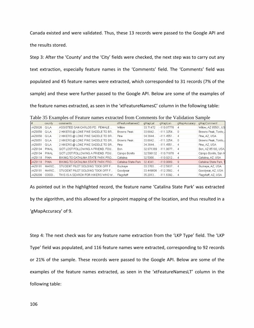
106

Canada existed and were validated. Thus, these 13 records were passed to the Google API and

the results stored.

Step 3: After the ‘County’ and the ‘City’ fields were checked, the next step was to carry out any

text extraction, especially feature names in the ‘Comments’ field. The ‘Comments’ field was

populated and 45 feature names were extracted, which corresponded to 31 records (7% of the

sample) and these were further passed to the Google API. Below are some of the examples of

the feature names extracted, as seen in the ‘xtFeatureNamesC’ column in the following table:

Table 35 Examples of Feature names extracted from Comments for the Validation Sample

As pointed out in the highlighted record, the feature name ‘Catalina State Park’ was extracted

by the algorithm, and this allowed for a pinpoint mapping of the location, and thus resulted in a

‘gMapAccuracy’ of 9.

Step 4: The next check was for any feature name extraction from the ‘LKP Type’ field. The ‘LKP

Type’ field was populated, and 116 feature names were extracted, corresponding to 92 records

or 21% of the sample. These records were passed to the Google API. Below are some of the

examples of the feature names extracted, as seen in the ‘xtFeatureNamesLT’ column in the

following table:

107

Table 36 Examples of Feature names extracted from LKP Type for the Validation Sample

Similar to the earlier case, as shown in the highlighted record, the feature name ‘Reef

Campground’ in Cochise county was extracted, resulting in the highest geocoding accuracy.

Step 5: A check was made for any street address related information from the ‘Comments’ field.

Street addresses were extracted for 37 records or 8% of the sample, and passed to the Google

API. Below are some examples:

Table 37 Examples of Street Address information extracted from Comments for the Validation Sample

The street address extracted from the ‘Comments’ field is captured in the ‘road_string’ column

and for some records, the geocoding accuracy increases because of the street address

information which is accounted for by the Google API.

108

Step 6: The final check is for any street address information in the ‘LKP Type’ field. The SAR

Algorithm extracted street addresses from 30 records or 7% of the sample, and these records

were further passed to the Google API. Below are some examples:

Table 38 Examples of Street Address information extracted from LKP Type for the Validation Sample

As can be seen in the highlighted records, the street address was accurately extracted and thus

the geocoding accuracy for these 2 records is very high (8-9). Also, for the other records a

higher accuracy of 6 was seen, compared to an accuracy of 3-4 for records where no address

related information is extracted.

After getting the latitude and longitude for all the records sent to the Google API in each step,

the difference in the actual coordinates as against the outputted coordinates was calculated

and stored in an xml file. A utility “csv2kml” was used to convert the excel file into the ‘kml’

format, which can be read by Google Earth. Finally all the points were plotted on Google Earth,

as shown below:

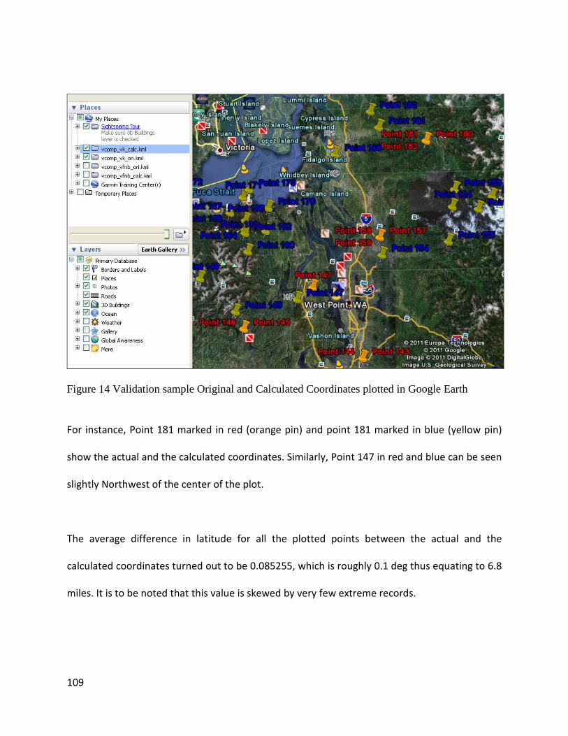
109

Figure 14 Validation sample Original and Calculated Coordinates plotted in Google Earth

For instance, Point 181 marked in red (orange pin) and point 181 marked in blue (yellow pin)

show the actual and the calculated coordinates. Similarly, Point 147 in red and blue can be seen

slightly Northwest of the center of the plot.

The average difference in latitude for all the plotted points between the actual and the

calculated coordinates turned out to be 0.085255, which is roughly 0.1 deg thus equating to 6.8

miles. It is to be noted that this value is skewed by very few extreme records.

110

Thus, based on the validation sample of 447 records out of the 2152 instances, it can be seen

that around 55-60% of the records are able to be geocoded purely based on the primary

address fields. Also, 10-15% of the records can be further geocoded to a higher accuracy by

extracting the address-related information from the textual fields. And finally, about 25-30% of

the records are unable to be geocoded in the Validation sample.

Figure 15 SAR Algorithm Geocodable break-up of records for the Validation sample

111

CHAPTER 6: FINDINGS & DISCUSSION

To summarize the SAR dataset, there were numerous instances of incomplete or missing data,

rendering some of the potential fields for analysis unusable. The data also was inaccurate and

inconsistent, with quite some useful information captured in textual fields. Essentially, the goal

was to come up with an algorithm to not only overcome the data quality issues, but use as

much as information as possible to geocode the LKP, either fully or partially.

Challenges faced in the SAR Study

Because of the nature of the dataset, there were a lot of factors or variables affecting the data

quality of the arrived LKP, apart from the issue of incomplete, inconsistent, invalid and

inaccurate data. For instance, there was individual address specific information which needed

to be looked at in the data quality perspective, such as street aliases, numeric county data as

against as county names, lack of street suffixes or prefixes, etc. in the text fields. Another factor

was the issue of dealing with some unknown information, such as the Zone details for UTM

coordinates, or the zip code information, to be specific. There was also the constraint of the

geocoding software used, in terms of accuracy, format and output constraints.

The level of inconsistency in the LKP coordinate fields was very high. As highlighted in the SAR

dataset examples, some regions of the world have a wide variation in the way the coordinates

were specified (“Land Information New Zealand: Datums, Projections & Heights,” n.d.). Thus, it

112

was not feasible to fully understand and identify the conversion rules for different formats for

all the regions in the dataset.

There was also the issue of misspelled words in information extraction from text fields, which,

because of the scope of the research and in light of the research objectives set, could not be

sufficiently dealt with. For example, extracting street address information from the textual

fields, either ‘Comments’ or the ‘LKP Type’ was very important in achieving the goal of fully

geocoding the LKP, as well as arriving at a much higher geocoding accuracy. However, although

the algorithm extracted street address information, the errors in either street address names,

or missing street prefixes and suffixes, or typos or extra characters in the address text, etc. in

such extracted text, could result in the possibility of no matches with the Google API’s address

database. Hence in such instances, the extracted information is not useful. Also, often, street

names in the US have street aliases and to give an example, ‘Alafaya Trail’, one of the streets in

Orlando, Florida is also called as ‘SR 434’, which stands for ‘State Road 434’.

Figure 16 Geocoding 'Alafaya Trail, Orlando, FL'

113

Figure 17 Geocoding 'SR 434, Orlando, FL'

Figure 18 Geocoding 'State Road 434, Orlando, FL'

114

As seen in the above figures, when specified in Google maps, the three different ways of

specifying the street each highlight a different part of its long stretch. Thus, if an alias was

mentioned in the text, with some missing details such as the street prefix, say, this could be the

cause of a variation in the geocoding accuracy.

At times, there is numeric data after the street address information in the textual fields, for

instance ‘FS ROAD 1170’ and hence it cannot be confidently said whether the actual address is

‘1170 FS ROAD’ or it might also be that ‘FS ROAD 1170’ is the actual street name. Thus, there

might be different results based on such errors, if they are in fact errors. As seen in the above

table, for the key# as US-AZ0232, ‘FS ROAD’ has been extracted with the accuracy of the

outputted coordinates being 9.

Table 39 Extracting street address information

Another example is information such as ‘PERALTA TRAIL HEAD’ in the ‘Comments’ field. The SAR

Algorithm is designed to truncate the extracted street address string or the ‘road_string’ at the

street suffix, since typical address information at the street level is expressed as the street

number, street prefix, street name and then the street suffix in that order. Thus when it

115

encounters information such as ‘Peralta Trail head’ somewhere in the text, it extracts ‘Peralta

Trail’ and since a street is a longer and less accurate than a trail head, which is a precise

location, the geocoding accuracy might be compromised. As can be seen in this instance, for

the record with the key# as US-AZ0083, the geocoding accuracy is 6.

Also, the feature names which are extracted from the textual fields should be extracted based

on the context and not purely based on a match. For instance, one of the feature names is a

placed called ‘Contact’, and the textual fields have lot of occurrences of the word ‘contact’

which is mainly used as a verb, as in ‘subject tried to contact the Park Rangers’, and thus this

resulted in false positives.

The algorithm was validated by selecting a sample size from those records where the LKP

coordinates had been populated, and then retaining the important fields while leaving the LKP

coordinate fields out. One of the reasons for being unable to select a larger sample was that of

those records where the coordinates were known, many did not have any substantial data in

the important fields, and hence those records would not be able to validate the SAR algorithm

which uses the data in the important fields to arrive at the LKP. Also, out of those records which

had the coordinates as well as the important fields populated, there was a lot of inconsistency

across the coordinate formats, as well as data quality issues with say, the Easting coordinate

populated in the Northing field and vice versa, or both the Northing and the Easting coordinate

populated in the Northing field, etc. Thus, out of the smaller subset of records where the LKP

coordinates were populated, were checked to be consistent and accurate, and where the other

116

fields were also populated, a sample was selected by querying the database and the first 447

records returned formed the sample.

Despite some of the above mentioned challenges, the SAR algorithm successfully geocoded 55-

60% of the data at a partial level purely based on the address fields and another 15% of the

data at a higher level of accuracy based on the overall aggregated address data through all the

concerned fields. Essentially majority of the data, around 70 – 75% of the data was successfully

geocoded. The remaining 20-25% of the data, which was unable to be geocoded at all, was

because of incomplete information in the important fields, especially the County, City and the

Comments field. Lack of any data whatsoever in these fields was the primary reason for no

geocoding at all for such records, as also issues of data quality where the data had been

populated.

Geocoding Accuracy Output Approach for validating the SAR algorithm

Goal: To arrive at the geocoding accuracy of records based on the Accuracy level output by the

Google API

Sample size chosen: 447, same as the earlier Validation set

To validate the SAR Algorithm using this approach, all the records are initially passed to the

Google API to be geocoded, based on only the address fields in the data. Thus, the address

string is formed by aggregating just the data source, which specifies the country (and also the

117

state, if it is a US record), county and city. The entire sample size of 447 is sent to the Google

API, and all the output variables, especially the Geocode Accuracy are captured.

The next step is to now run the SAR Algorithm on the same sample dataset, by traversing the

SAR flowcharts described in the earlier sections, and passing all the records based on individual

criteria to the Google API. The output variables are captured as before, and further compared

to the output on the same data before the SAR Algorithm is used. The Geocoding accuracy by

the Google API takes on values 0 through 9, where 0 represents an unknown accuracy. Thus,

the accuracy increases from a level of 1, which represents Country level accuracy upto a level of

9, which represents the highest accuracy, i.e. a premise (building name, shopping center, etc.)

accuracy. It is to be noted that Google mentions the accuracy field being more the order of

resolution of an address than its correctness, however since the LKP coordinates for the

validation set are populated, and since the plotting validation accuracy has already been tested,

the accuracy level output by the Google API does indeed reflect the accuracy of geocoding

using the SAR Algorithm.

Here is a table of the accuracy levels and their descriptions:

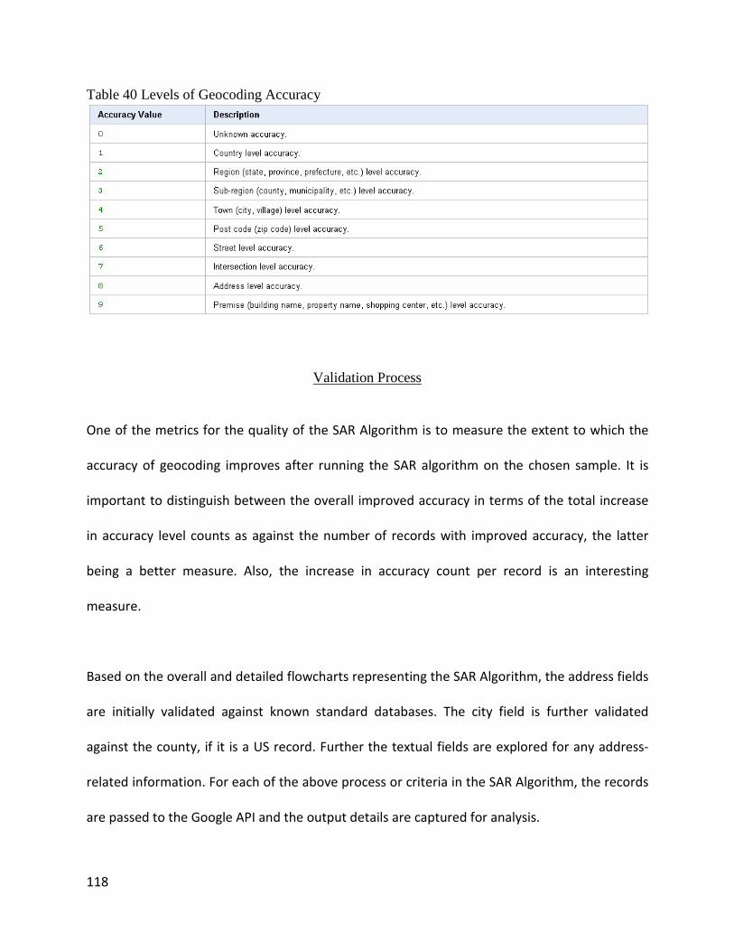
118

Table 40 Levels of Geocoding Accuracy

Validation Process

One of the metrics for the quality of the SAR Algorithm is to measure the extent to which the

accuracy of geocoding improves after running the SAR algorithm on the chosen sample. It is

important to distinguish between the overall improved accuracy in terms of the total increase

in accuracy level counts as against the number of records with improved accuracy, the latter

being a better measure. Also, the increase in accuracy count per record is an interesting

measure.

Based on the overall and detailed flowcharts representing the SAR Algorithm, the address fields

are initially validated against known standard databases. The city field is further validated

against the county, if it is a US record. Further the textual fields are explored for any address-

related information. For each of the above process or criteria in the SAR Algorithm, the records

are passed to the Google API and the output details are captured for analysis.

119

Some of the column names for the output tables generated are as follows:

gMapStringPassed is the address string sent initially to the Google API without applying the SAR

Algorithm on the sample.

SB_gMapStringPassed is the address string passed after feature names have been extraction

from Comments

FNA_gMapStringPassed is the address string sent to the Google API after street address

information has been extracted from LKP Type.

Here are the output tables for each SAR Algorithm path:

120

Table 41 Validating the 'City'(C) field

Table 42 Validating the 'County'(K) field

121

Table 43 Extracting Feature Names(FNA) from the 'Comments' field

122

Table 44 Extracting Feature Names(FNB) from the 'LKP Type' field

123

Table 45 Extracting Street address information(SA) from the 'Comments' field

124

Table 46 Extracting Street address information(SB) from the 'LKP Type' field

125

SAR Algorithm Analysis

Validating the 'City'(C) field

In the validation sample, most of the 'City' fields are not populated. Only 13 records have 'City'

information, and all cities were invalid, which were validated by the SAR Algorithm. As can be

seen in Table 41, although the gain in accuracy is 4 records, it is 4/13, which is quite high, and

thus validating individual address fields before geocoding is an important data cleaning phase.

Validating the 'County'(K) field

The 'County' fields were all populated for the validation sample, and also it was seen that 389

out of 447 instances were counties which were valid. The other 58 instances had some dirty

instances and other information, because of which those fields could not be cleaned. Thus since

most of the counties were valid to begin with, the SAR Algorithm was unable to improve the

accuracy at all, considering the criteria of validating the 'County' field.

Extracting Feature Names(FNA) from the 'Comments' field

Here, although quite some feature names were extracted, often they were either the city or the

county specified in the comments, and hence did not add to the address information to be

126

passed to the Geocoding API. At the same time, whenever there was any specific feature name

such as 'Catalina State Park', the API used such information extracted to geocode to the highest

level of accuracy, as seen in the last example highlighted in the Table 42. Thus the gain in

accuracy was 19 records.

Extracting Feature Names(FNB) from the 'LKP Type' field

Quite some feature names were extracted from the LKP Type field, some of which were specific

while others were again city or county names. This criterion contributed to the largest gain in

accuracy, which was 36 records

Extracting Street address information from the 'Comments' field

The street address information when extracted, either contributed to an increased accuracy, or

sometimes a drop in accuracy. When extracting street suffix information such as 'Road' in the

textual fields, if a lot of non-address data is extracted, such as 'drove off road', then the Google

API has too much of garbled information to process the long address string, and hence the

accuracy suffers. Only 5 records had a gain in accuracy using this criterion.

127

Extracting Street address information from the 'LKP Type' field

Although the number of records which showed a gain in accuracy was 20, the level of accuracy

achieved after running the algorithm and extracting address information from LKP Type was

quite high. As can be seen in Table 45, the last three records are geocoded to an accuracy of 8

and 9. In the record with the key# as 'US-AZ0147', when '1957 Montana Rd' was extracted, the

accuracy doubled from a 4 to a 8.

Results and Discussion

Here are the results summarized:

Number of records with a Gain in Accuracy due to:

City validation (C): 04

County validation (K): none

Feature Names extracted from Comments (FNA): 19

Feature Names extracted from LKP Type (FNB): 36

Street address extracted from Comments (SA): 05

Street address extracted from LKP Type (SB): 20

Total Gain of Accuracy in the Sample: 84

% of records with a gain in accuracy: 84/447= 18.7919%

128

Thus, it was seen that there was almost a 19% increase in the number of records which were

able to be geocoded with a better resolution and precision by running the SAR Algorithm. Often

the tables above show a negative gain. This is because some of the city or county level

geocoded records have 0 as their accuracy, which represents an unknown accuracy. Thus if the

accuracy without the SAR algorithm is at 2 or 3, and although the records get geocoded, if some

of them have '0' as their accuracy, there is negative gain, and hence negative gain is not so

much focused on here. Another way these results can be tested or visualized using kml files and

plotting them on Google Earth, to show the accuracy of the plots for each case, with and

without running the SAR Algorithm.

Improving the SAR Algorithm Accuracy

The accuracy of the SAR Algorithm using this approach can be further improved by the

following:

Incorporating all street suffixes available using the USPS Street Suffix Standard or some other

known Street Specification. For this validation sample, just a few suffixes such as 'road', trail',

'st', 'lake', 'creek', etc. were used.

Another way to improve the accuracy is to avoid non-address information being passed as the

gMapStringPassed to the Google API. For instance, some words such as ‘of’, ‘off’, ‘along’, ‘lying’,

etc. in the context of 'road' could be avoided, in an effort to extract only valid address

129

information. Thus, the text extraction can be further refined by adding such context or business

rules.

Different combinations of the fields used to form the address string to be passed to the API can

be used. For instance, if the extracted text information comes up with no match as in the 'drove

off road' example, where the SAR Algorithm looks for instances of street suffixes, and instead

gets a '0' accuracy, the algorithm can resend the address information by removing the

extracted text, and just sending the city or county level information, so that a reasonable

geocoding accuracy of 3 or 4 can be achieved.

Thus, the SAR Algorithm makes use of partial or incomplete information residing in the

database, identifies dirty data based on the domain business rules and other applied rules,

cleans the data in the relevant fields, validates the data against accurate data, further cross-

checks the data against multiple sources, and successfully geocodes the data.

Findings from Data Quality Work in Other Domains

The previous completed work some of which was applied to the SAR dataset has been

summarized below:

(Some of the research methodologies used was to target a different set of data domains, and

devise techniques for analyzing and improving the data quality)

130

Business Logic framework for the Vehicle Identification Number (VIN)

This research stemmed from the specific need to validate data input that follows complex rules

requiring both enumerations and conditional decisions based on the enumerations. The dataset

chosen was the VIN dataset, which is a complex one, since the VIN number is governed by

business rules, requiring it to satisfy both conditionals as well as enumerations for its validation.

These rules depend on a multitude of factors such as the manufacturer, the country of

manufacture, the vehicle make, the vehicle model, etc. to highlight a few. Also, there exist

different rules for specified digit positions in a VIN. Another characteristic of the VIN dataset,

when it comes to validation is that a single VIN can be validated against fixed business rules.

The goal for the research was to explore the sole use of regular expressions in validating the

VIN dataset. By taking the Vehicle Identification Numbers or VINs as an example, a flexible and

scalable business logic framework was provided for validating such a complex dataset against a

specified rule-set. The framework encapsulated the numerous business rules in the form of

regular expressions, which are stored in a database. Being generic, such a framework can be

successfully extended to data having similar characteristics such as driver license numbers,

insurance id numbers, etc., where the input validation can be carried out solely on a single-

field, without considering any other related data fields.

This specific part of the research carried out meets the 2nd, 3rd and 4th objective listed in the

‘Objectives’ section.

131

Technique for Measuring Data Quality of Person Names as applied to Pawn data

One of the challenges in criminal datasets is to identify whether two suspects having ‘similar’

names are indeed the same person. Often, when crime-related databases are queried against a

particular name, the query results return a large number of similar suspect names. The goal for

this research was to develop an algorithm to identify the extent of dirtiness pertaining to

person names, and measure it in a quantifiable manner.

The data used in this study came from a criminal records database called FINDER (Florida

Integrated Network for Data Exchange and Retrieval). The accuracy of data was measured by

defining data quality metrics for some of the data elements, and finally arriving at the database

cleanliness score for the entire database. The research contributed to the field by developing a

Data-Cleanliness algorithm, which makes use of the 'Levenshtein distance', to measure the data

quality for a criminal records database. The proposed algorithm demonstrates how one can

arrive at the dirtiness measure of any database, which not only helps in setting up guidelines

for the data clean-up process, but also helps in cross-comparing dirtiness measures across

different datasets.

The potential for future work here is to carry out a sensitivity analysis by varying the weights

assigned to the different variables, across similar datasets. This shall identify as to what extent

each variable impacts the desired outcome, and thus help in refining the algorithm.

132

Data Cleanliness Techniques applied to the Seminole County Address data

The research focused on the data preparation or data cleaning phase for the Seminole County

Address Database, which mostly contained various geographical fields, each of which specified

the address information, such as street prefixes, street names, street suffixes, city names,

states and the zip codes.

The initial work involved gaining a general insight into the data quality of the Address data, by

running some general queries, and further understanding the business rules specific to the

Seminole County Address data. The cleaning phase was divided into two phases called ‘Simple

Clean’ and ‘Final Clean’. ‘Simple Clean’ involved automating the data cleaning process, where

the business rules had a strong level of clarity, and could be incorporated conveniently.

However, for specific dirtiness instances, where the business rules alone weren’t sufficient to

arrive at a data quality decision, and where human intervention was necessary, the ‘Final Clean’

phase of the cleaning process flagged such records, and further actions were taken by the

authorized personnel and knowledgeable domain experts in the field.

This specific part of the research focused on developing algorithms for automated cleaning of

the real-life address data at the Seminole County, based on the business rules, wherever

possible, and highlighting instances where the data was known to be dirty. The insights into

address gained in this study were very helpful in developing some of the aspects of the SAR

Algorithm.

133

String Matching Algorithm as applied to Burglary data

Although techniques such as Soundex, Phonix, N-grams, edit distance, have been used to

improve the matching rate in these name-matching applications and have demonstrated

varying levels of success, the research for this study focuses on the need for name matching

approaches that provide high levels of accuracy, while at the same time maintaining low

computational complexity.

A string-matching algorithm which is fast, accurate and scalable to large databases was

proposed - ANSWER (Approximate Name Search With ERrors). The algorithm relies on the ‘Edit

Distance’ or the ‘Levenshtein’ algorithm, and the innovation lies in the fact that the entire

database doesn’t have to be searched in order to find names matching a given query. This is

accomplished by building a dictionary of names. Thus, in order to reduce the time complexity of

the full-search of partially matching names in the database, the PREFIX algorithm constructs a

structured dictionary or a tree of prefixes corresponding to the existing names in the database.

Searching the tree structure is a lot more efficient than searching the entire database. The

ANSWER algorithm takes every full name in the database, and using the PREFIX algorithm, it

creates required nodes and links for the last names in the tree, and thus the search time is

greatly reduced.

134

Relevance of this Study

A lot of engineering applications generate huge quantities of data, requiring a thorough analysis

for improved decision making. The study clearly and convincingly demonstrates and addresses

the critical need for identifying data cleanliness issues, measuring data quality and monitoring it

for any engineering application which relies on data.

For data domains as diverse the ones explored in this study such as the Burglary data, Person

Data, Address data, VIN data, and the SAR data, the data quality approaches, techniques and

the algorithms developed can be readily and extensively applied to similar datasets. The

Answer Algorithm improves on some of the other name-matching algorithms. The Data

Cleanliness Algorithm devised actually quantifies data cleanliness and thus arrives at a number

representing the data quality of the database, which is an excellent metric for data quality. The

Business Logic Framework making use of regular expressions for validating data at data entry is

a novel approach and very generic in that it can be implemented for any data, which have their

own self-contained rules. The SAR Algorithm handles partial or incomplete data, and cleans,

validates the data so as to arrive at the goal of geocoding the LKP.

This study has met all the research goals and objectives outlined in the proposal phase, and can

be effectively used for handling data quality issues in various engineering applications.

135

Future Work

Some of the ways in which the SAR Algorithm can be further refined and improved upon are

described below:

The algorithm can be applied on a much larger dataset, which would help several unique and

interesting cases, with regards to say, the LKP geocoding accuracy, or highlight certain fields

which can be potentially used to extract address information, etc. It could also help identify

data patterns, if any, which probably could not be visualized because of the smaller dataset.

Also, the validation sample size would be correspondingly larger for a larger dataset, thus

enabling an understanding as to what extent the percentage of records which can be fully,

partially, or unable to be geocoded vary.

The present SAR dataset had 80 % of the data about SAR incidents that happened in the US,

and the remaining 20% split among countries such as Canada, Australia, New Zealand, UK and

South Africa. There exist several coordinate format inconsistencies across various states in the

US and then specific cases about New Zealand. If the dataset pertains to several other

countries, implying a high number of data points for each country, it would be worthwhile to

carry out a detailed analysis on the coordinate formats used in each particular country and the

variations therein and thus arrive at the rules for conversion. For the SAR dataset, the validation

sample could have been a lot larger, if some of the rules for conversion could have been

identified for the rest of the countries in the dataset.

136

Since there are several different software which can be used for geocoding the LKP other than

the one used for this research, namely the Google API, it would be worthwhile and interesting

to compare the geocoding accuracy for each of these software on the same data, and also to

identify pros and cons of using one over the other.

Another research area is to analyze how formatting and structuring the ‘address string’ to be

passed to the Google Geocoding API affects first of all, the geocode output, and secondly the

geocoding accuracy.

The ‘Comments’ field in the SAR dataset, contains quite a lot of information about the SAR

incident, and the focus of this research specifically being to geocode the LKP, only the address-

related information was extracted from the textual fields. However in future, a text mining

component could be incorporated in the algorithm so as to qualitatively extract as much SAR

incident information as possible. One of the beneficial aspects is that the information so

extracted can be used to impute missing values and thus complete some of the unknown or null

fields in the database.

137

REFERENCES

Abi-Zeid, I., & Frost, J.R. (2005). SARPlan: a decision support system for canadian search and rescue operations. European Journal of Operational Research 162, 630–653.

Adams, A.L., Schmidt, T.A., Newgard, C.D., Federiuk, C.S., Christie, M., Scorvo, S., & DeFreest, M. (2007). Search is a time-critical event: when search and rescue missions may become futile. Wilderness and Environmental Medicine, 18(2):95-101. doi: 10.1580/06-WEME-OR-035R1.1

Bayesian Models for Search and Rescue. (n.d.). Retrieved from http://sarbayes.org/index.shtml

Benchmark. (2006). Kalido continues rapid expansion and reports record year of growth - enterprise data warehouse and master data management provider records best year to date. Retrieved from http://www.balderton.com/news-events/kalido-continues-rapid-expansion-and-reports-record-year-of-growth--enterprise-data-warehouse-and-master-data-management-provider-records-best-year-to-date,,59/

Bex, G.J., Gelade, W., Neven, F., & Vansummeren, S. (2008). Learning deterministic regular expressions for the inference of schemas from xml data. WWW 2008, China.

Brabrand, C., Moller, A., Ricky, M., & Schwartzbach, M.I. (2000). Powerforms: declarative client-side form field validation. Retrieved from http://www.daimi.au.dk/~brabrand/powerforms.pdf

Brundick, F.S. (2009). Performing xml data validation in the global force management data initiative. Retrieved from http://www.dtic.mil/cgi-bin/GetTRDoc?Location=U2&doc=GetTRDoc.pdf&AD=ADA494863

Caro, J. & Prieto, M. (2010) GNSS support to canine search and rescue. Retrieved from http://mycoordinates.org/gnss-support-to-canine-search-and-rescue/

Carter, B. A., Hubert, L. A., and Walton, A. C. (2007). Applications of regular expressions. Retrieved from http://citeseerx.ist.psu.edu/viewdoc/download?doi=10.1.1.138.4212&rep=rep1&type=pdf

Cibola coordinate systems conversion resource. (n.d.). Retrieved from http://www.cibolasar.org/UTMConverter.shtml

Conzelmann, C.P., Sleavin, W., & Couvillion, B. (n.d.). Using geospatial technology to process 911 calls after hurricanes katrina and rita. Retrieved from http://pubs.usgs.gov/circ/1306/pdf/c1306_ch3_b1.pdf

Cooper, D. (2005). Fundamentals of search and rescue. Massachusetts: Jones & Bartlett Learning.

Cox, J. (2002). Working out the bugs in xml databases. Retrieved from http://www.networkworld.com/news/2002/0107specialfocus.html

Crosier, S. (2004). ArcGIS 9. geocoding in arcgis. California: ESRI Press.

138

Dai, B.T., Koudas, N., Ooi, B.C., Srivastava, D., & Venkatasubramanian, S. (2006). Column heterogeneity as a measure of data quality. CleanDB, Korea.

Dasu, T., Vesonder, G.T., & Wright, J.R. (2003). Data quality through knowledge engineering. SIGKDD ’03, 1-58113-737-0/03/0008.

Davidson, I., Grover, A., Satyanarayana, A., & Tayi, G.K. (2004). A general approach to incorporate data quality matrices into data mining algorithms. KDD’04, 1-58113-000-0/00/0004.

Davis, R. (2003). Adding regular expressions to your cocoa application. Retrieved from http://www.mactech.com/articles/mactech/Vol.19/19.04/RegularExpressions/

Dehaan, P. (n.d.). Validating data using regular expressions. Retrieved from http://blog.flexexamples.com/2007/08/22/validating-data-using-regular-expressions/

Dramowicz, E. (2004). Three standard geocoding methods. Retrieved from http://www.directionsmag.com/articles/three-standard-geocoding-methods/123627

Federal Emergency Management Agency. (n.d.). Retrieved from http://www.fema.gov/index.shtm

Forta, B. (2004). Sams teach yourself regular expressions in 10 minutes. Indiana: Sams Publishing.

Friedl, J.E.F. (1997). Mastering regular expressions. California: O'Reilly Media.

Friedman, T., Bitterer, A., & Hostmann, B. (2006). Focus on data quality in bi motivates business objects. Retrieved from http://www.gartner.com/DisplayDocument?id=489320&ref=g_sitelink

Garofalakis, M.N., Rastoji, R., & Shim, K. (1999). SPIRIT: sequential pattern mining with regular expression constraints. Proceedings of the 25th VLDB Conference, Scotland.

Gelman, I.A. (2010). Setting priorities for data accuracy improvements in satisficing decision-making scenarios: a guiding theory. Decision Support Systems, 48, 507-520. doi:10.1016/j.dss.2009.11.001

Girven, C. (n.d.). Cibola search and rescue gps test. Retrieved from http://www.cibolasar.org/GPS_Study/GPS_study.pdf

Hackett, B., Breivik, O., & Wettre, C. (n.d.). Forecasting the drift of objects and substances in the ocean. In GODAE Book (chapter 23). Retrieved from http://www.coaps.fsu.edu/pub/eric/RSMAS/GODAE_School/GODAE_Book/Chap23-Hackett.pdf

Hagland, M. (2004). Stronger computer tools allow deeper analysis of medical research, patient care and insurance data. Healthcare Informatics. 21(4), 33-6.

Heggie, T.W., & Amundson, M.E. (2009). Dead men walking: search and rescue in US national parks. Wilderness and Environmental Medicine, 20, 244–249.

Heggie, T.W., & Heggie, T.M. (2008). Search and rescue trends and the emergency medical service workload in utah’s national parks. Wilderness and Environmental Medicine, 19, 164 171.

139

Heggie, T.W., & Heggie, T.M. (2009). Search and rescue trends associated with recreational travel in us national parks. Journal of Travel Medicine, Volume 16, Issue 1, 23–27. doi: 10.1111/j.1708-8305.2008.00269.x

Heggie, T.W., & Heggie, T.M. (2008). Search and rescue trends and the emergency medical service workload in utah’s national parks. Wilderness and Environmental Medicine, 19, 164 171.

Heth, C.D., Dostatni, G., & Cornell, E.H. (n.d.). Spatial decision support for urban search and rescue and disaster management. Retrieved from http://geoanalytics.net/VisA-SDS-2006/paper20.pdf

Hipp, J., Guntzer, U., & Grimmer, U. (2001). Data quality mining, making a virtue of necessity. DMKD.

Hosoya, H., & Pierce, B.C. (2003). Regular expression pattern matching for xml. Journal of Functional Programming, Volume 13, Issue 6, pages 961-1004.

Hung, E.K., & Townes, D.A. (2007). Search and rescue in yosemite national park: a 10-year review. Wilderness and Environmental Medicine, 18, 111-116.

IBM Research. (n. d.). Online data continues to grow at an explosive pace. Retrieved from http://domino.research.ibm.com/comm/research.nsf/pages/r.kdd.spotlight.html

Imhoff, C. (2006). Poor-quality data… can your company afford the risk. Retrieved from http://www.teradata.com/library/pdf/ar4759.pdf

Informatica White Paper. Addressing data quality at the enterprise level. Retrieved from http://pdf.me.uk/informatica/AAHN/INF13.pdf

Kim, W. (2002). On three major holes in data warehousing today. Journal of Object Technology - JOT, 1(4), 39-47.

Kim, W., Choi, B., Hong, E., Kim, S., & Lee, D. (2003). A taxonomy of dirty data. Data Mining and Knowledge Discovery, 7, 81–99, 2003.

Kursun, O., Koufakou, A., Wakchaure, A., Georgiopoulos, M., Reynolds, K., & Eaglin, R. (2006). ANSWER: approximate name search with errors in large databases by a novel approach based on prefix-dictionary. International Journal on Artificial Intelligence Tools, Vol. 15, No.5 (2006) 839-848.

Land Information New Zealand: Datums, Projections & Heights. (n.d.). Retrieved from http://www.linz.govt.nz/geodetic/datums-projections-heights

Leahy, T. (n.d.). Better data, better performance management. Retrieved from http://www.businessfinancemag.com/magazine/archives/article.html?articleID=13956.

Lee, M., Hsu, W., & Kothari, V. (2004). Cleaning the spurious links in data. IEEE Intelligent Systems, 1094-7167/04.

Leitheiser, R.L. (2001). Data quality in health care data warehouse environments. Proceedings of the 34th Hawaii International Conference on System Sciences, 0-7695-0981-9/01.

140

Lerner, R. (n.d.). Data quality by the numbers: Best practices for managing business data. Retrieved from http://www.dataflux.com

Levenshtein, V.L. (1966). Binary codes capable of correcting deletions, insertions, and reversals. Soviet Physics, Doklady, vol. 10, pp. 707–710.

Lewis, L. (2002). Quick levenshtein edit distance. Retrieved from http://www.planet-source-code.com/vb/scripts/ShowCode.asp?txtCodeId=584&lngWId=5

Linsley, P., & Trute, B. (n.d.). Introducing oracle regular expressions. Retrieved from http://www.oracle.com/technology/products/database/application_development/pdf/TWP_Regular_Expressions.pdf

Lowe, R.(n.d.). Common applications of regular expressions. Retrieved from http://www.4guysfromrolla.com/webtech/120400-1.shtml

Maddock, J. (2001, October). Regular expressions in C++. Dr.Dobb’s. Retrieved from http://drdobbs.com/cpp/184404797.

Martin, M. (2005). Measuring and improving data quality, part ii: measuring data quality. Retrieved from http://nsu.aphis.usda.gov/outlook/issue5/data_quality_part2.pdf

McIntosh, S.E., Brillhart, A., Dow, J., & Grissom, C.K. (2010). Search and rescue activity on denali, 1990 to 2008. Wilderness and Environmental Medicine, 21, 103–108.

McKnight, W. (n.d.). Overall approach to data quality ROI, first logic white paper. Retrieved from http://www.utopiainc.com/pdfs/OverallApproachtoDataQualityROI.pdf

Meier, J.D., Mackman, A., Wastell, B., Bansode, P., and Wigley, A. (2005). How to: use regular expressions to constrain input in asp.net. Retrieved from http://msdn.microsoft.com/en-us/library/ff650303.aspx

Moad, J. (2003). Mopping up dirty data. Retrieved from http://www.baselinemag.com/article2/0,1540,1438233,00.asp

Muller, H., Leser, U., & Freytag, J. (2004). Mining for patterns in contradictory data. IQIS, 1-58113-902-0/04/0006.

National Response Framework by FEMA. (n.d.). Retrieved from http://www.fema.gov/emergency/nrf/

Paulson, L. D. (2000). Data quality: a rising e-business concern, IT Professional, 2(4), 10-14.

Pierce, E.M. (2004). Assessing data quality with control matrices. Communications of the ACM, Vol. 47, No. 2.

Pipino, L.L., Lee, Y.W., & Wang, R.Y. (2002). Data quality assessment. Communications of the ACM, Vol. 45, No. 4ve.

141

Rahm, E., Do, H. (n.d.). Data cleaning: problems and current approaches, University of Leipzig, Germany. Retrieved from http://wwwiti.cs.uni-magdeburg.de/iti_db/lehre/dw/paper/data_cleaning.pdf

RCN Utilities & Tools. (n.d.). Retrieved from http://www.rcn.montana.edu/resources/tools/coordinates.aspx

Redman, T.C. (1998). The impact of poor data quality on the typical enterprise. Communications of the ACM, Vol. 41, No. 2.

S.E.T.T.L.E.R. pod factoring and reporting, monitoring probability of success [PowerPoint Slides]. (2005). Retrieved from http://www.podfactoring.org/SETTLER%20PODfactoringv2010.2.ppt

Scaffidi, C., Myers, B., & Shaw, M. (2008). Tool support for data validation by end-user programmers. Proceedings of the ICSE’08, Germany.

Scaffidi, C., Myers, B., & Shaw, M. (2008). Topes: reusable abstractions for validating data. ICSE, Germany.

Schiff, M. (n.d.). Data quality first: its just logical. Retrieved from http://www.dsstechnology.com/Portals/0/DSSDownload/EIM/WP_DQ_EIM.pdf

Shafer, J. (2010). The bogusity of the new york times' story about how technology leads more park visitors into trouble. Retrieved from http://www.slate.com/id/2264778/

Shah, H.C. (2003). Regular expressions in j2se. Retrieved from http://onjava.com/pub/a/onjava/2003/11/26/regex.html

Smalltree, H. (2006). BIs seven fatal flaws. Retrieved from http://searchdatamanagement.techtarget.com/originalContent/0,289142,sid91_gci1172024,00.html

Soylemez, E. (2007). GIS-based search theory application for search and rescue planning (Master’s thesis, The Graduate School of Natural and Applied Sciences of Middle East Technical University, Ankara, Turkey). Retrieved from http://etd.lib.metu.edu.tr/upload/12608362/index.pdf

Tabladillo, M. (2005). Mapping an Exclusive Regular Expression Strategy. Proceedings of the 30th SAS User Group International Conference, Paper 178-30.

The Google Geocoding API. (n.d.). Retrieved from http://code.google.com/apis/maps/documentation/geocoding/

The National Association for Search and Rescue. (n.d.). Retrieved from http://www.nasar.org/

Theodore, J. (2009). When every second counts, yosemite uses gis for coordinating search and rescue operations. Retrieved from http://www.esri.com/news/arcuser/0609/yosar.html

Vaas, L. (2005). Which is scarier: Dirty data in the hands of the fbi or bloggers? Retrieved from http://www.eweek.com/c/a/Database/Which-Is-Scarier-Dirty-Data-in-the-Hands-of-the-FBI-or-Bloggers/

142

Vries, S. (2006). A modular approach to data validation in web applications. Retrieved from http://research.corsaire.com/whitepapers/060116-a-modular-approach-to-data-validation.pdf

Watts, S., Shankaranarayanan, G., & Even, A. (2009). Data quality assessment in context: a cognitive perspective. Decision Support Systems, 48, 202-211. doi:10.1016/j.dss.2009.07.012

Welzer, T., Brumen, B., Golob, I. & Druzovec, M. (2002). Medical diagnostic and data quality. Proceedings of the 15th IEEE Symposium on Computer-Based Medical Systems (CBMS 2002), 1063-7125/02.

Wild, F.J. (2008). Epidemiology of mountain search and rescue operations in banff, yoho, and kootenay national parks, 2003–06. Wilderness and Environmental Medicine, 19(4):245-251.

Yu, F., Chen, Z., Diao, Y., Lakshman, T.V., & Katz, R.H. (2006). Fast and memory-efficient regular expression matching for deep packet inspection. Proceedings of the ANCS ’06, USA.