Embed Size (px)
Citation preview
Exploring novel
designs of NLP solvers
Architecture and Implementation of WORHP
by
Dennis Wassel
Thesis submitted to University of Bremen
for the degree of Dr.-Ing.
March 2013.
Date of Defense: 25.04.2013
1st referee: Prof. Dr. Christof Büskens
2nd referee: Prof. Dr. Matthias Gerdts
3rd examiner: Prof. Dr. Angelika Bunse-Gerstner
4th examiner: Dr. Matthias Knauer
Contents
List of Listings v
List of Figures vii
Foreword ix
1. Nonlinear Programming 11.1. Mathematical Foundations . . . . . . . . . . . . . . . . . . . . . . . . . . 21.2. Penalty and barrier methods . . . . . . . . . . . . . . . . . . . . . . . . . 71.3. Sequential Quadratic Programming . . . . . . . . . . . . . . . . . . . . . 9
1.3.1. Derivative Approximations . . . . . . . . . . . . . . . . . . . . . . 111.3.2. Optimality and Termination Criteria . . . . . . . . . . . . . . . . 181.3.3. Hessian Regularization . . . . . . . . . . . . . . . . . . . . . . . . 221.3.4. Prepare the Quadratic Problem . . . . . . . . . . . . . . . . . . . 231.3.5. Determine Step Size . . . . . . . . . . . . . . . . . . . . . . . . . 261.3.6. Recovery Strategies . . . . . . . . . . . . . . . . . . . . . . . . . . 30
2. Architecture of WORHP 312.1. Practical Problem Formulation . . . . . . . . . . . . . . . . . . . . . . . 332.2. Sparse Matrices . . . . . . . . . . . . . . . . . . . . . . . . . . . . . . . . 35
2.2.1. Coordinate Storage format . . . . . . . . . . . . . . . . . . . . . . 352.2.2. Compressed Column format . . . . . . . . . . . . . . . . . . . . . 36
2.3. Data Housekeeping . . . . . . . . . . . . . . . . . . . . . . . . . . . . . . 382.3.1. The traditional many arguments convention . . . . . . . . . . . . 392.3.2. The USI approach in Worhp . . . . . . . . . . . . . . . . . . . . 40
2.4. Reverse Communication . . . . . . . . . . . . . . . . . . . . . . . . . . . 432.4.1. Division into stages . . . . . . . . . . . . . . . . . . . . . . . . . . 442.4.2. Implementation considerations . . . . . . . . . . . . . . . . . . . . 462.4.3. Applications . . . . . . . . . . . . . . . . . . . . . . . . . . . . . . 48
2.5. Serialization . . . . . . . . . . . . . . . . . . . . . . . . . . . . . . . . . . 492.5.1. Hotstart functionality . . . . . . . . . . . . . . . . . . . . . . . . 49
i
Contents
2.5.2. Reading parameters . . . . . . . . . . . . . . . . . . . . . . . . . . 492.5.3. Serialization format . . . . . . . . . . . . . . . . . . . . . . . . . . 50
3. Technical Implementation 533.1. Hybrid implementation . . . . . . . . . . . . . . . . . . . . . . . . . . . . 55
3.1.1. Interoperability issues . . . . . . . . . . . . . . . . . . . . . . . . 553.1.2. Interoperability improvements . . . . . . . . . . . . . . . . . . . . 593.1.3. Data structure handling in Worhp . . . . . . . . . . . . . . . . . 63
3.2. Automatic code generation . . . . . . . . . . . . . . . . . . . . . . . . . . 683.2.1. Data structure deőnition . . . . . . . . . . . . . . . . . . . . . . . 693.2.2. Deőnition őle . . . . . . . . . . . . . . . . . . . . . . . . . . . . . 703.2.3. Template őles . . . . . . . . . . . . . . . . . . . . . . . . . . . . . 723.2.4. Applications of automatic code generation . . . . . . . . . . . . . 73
3.3. Interactive mode . . . . . . . . . . . . . . . . . . . . . . . . . . . . . . . 763.4. Workspace Management . . . . . . . . . . . . . . . . . . . . . . . . . . . 79
3.4.1. Automatic workspace management . . . . . . . . . . . . . . . . . 793.4.2. Dedicated dynamic memory . . . . . . . . . . . . . . . . . . . . . 81
3.5. Internal XML parser . . . . . . . . . . . . . . . . . . . . . . . . . . . . . 853.6. Established shortcomings, bugs and workarounds . . . . . . . . . . . . . 87
3.6.1. Intel Visual Fortran 10.1 . . . . . . . . . . . . . . . . . . . . . . . 873.6.2. Windows . . . . . . . . . . . . . . . . . . . . . . . . . . . . . . . . 87
3.7. Maintaining compatibility across versions . . . . . . . . . . . . . . . . . . 89
4. Solver Infrastructure 914.1. Conőguration and Build system . . . . . . . . . . . . . . . . . . . . . . . 92
4.1.1. Available build tools . . . . . . . . . . . . . . . . . . . . . . . . . 924.1.2. Basics of make . . . . . . . . . . . . . . . . . . . . . . . . . . . . . 944.1.3. Directory structure . . . . . . . . . . . . . . . . . . . . . . . . . . 954.1.4. Pitfalls of recursive make . . . . . . . . . . . . . . . . . . . . . . . 964.1.5. Non-recursive make . . . . . . . . . . . . . . . . . . . . . . . . . . 99
4.2. Version and conőguration info . . . . . . . . . . . . . . . . . . . . . . . . 1044.3. Testing Approach . . . . . . . . . . . . . . . . . . . . . . . . . . . . . . . 1074.4. Testing Infrastructure . . . . . . . . . . . . . . . . . . . . . . . . . . . . . 110
4.4.1. Parallel testing script . . . . . . . . . . . . . . . . . . . . . . . . . 1104.4.2. Solver output processing . . . . . . . . . . . . . . . . . . . . . . . 113
4.5. Parameter Tuning . . . . . . . . . . . . . . . . . . . . . . . . . . . . . . . 1164.5.1. Why tune solver parameters? . . . . . . . . . . . . . . . . . . . . 1164.5.2. Sweeping the Parameter Space . . . . . . . . . . . . . . . . . . . . 1174.5.3. Examples . . . . . . . . . . . . . . . . . . . . . . . . . . . . . . . 1204.5.4. Conclusions . . . . . . . . . . . . . . . . . . . . . . . . . . . . . . 127
4.6. Future directions for testing . . . . . . . . . . . . . . . . . . . . . . . . . 128
A. Examples 131A.1. Bypassing const-ness . . . . . . . . . . . . . . . . . . . . . . . . . . . . . 131
ii

Contents
List of terms 133
List of acronyms 141
Bibliography 143
iii

List of Listings
2.1. Interface of snOptA (the advanced SNOPT interface) . . . . . . . . . . . 382.2. User action query and reset . . . . . . . . . . . . . . . . . . . . . . . . . 48
3.1. Example of a non-standard Fortran data structure . . . . . . . . . . . . . 553.2. Example of a C-interoperable Fortran type . . . . . . . . . . . . . . . . . 603.3. C struct corresponding to the Fortran type in listing 3.2. . . . . . . . . 613.4. Snippet of the data structure deőnition őle . . . . . . . . . . . . . . . . . 703.5. Help output of interactive mode . . . . . . . . . . . . . . . . . . . . . . . 773.6. Detail help output of interactive mode . . . . . . . . . . . . . . . . . . . 783.7. Data hiding in plain C through incomplete types. . . . . . . . . . . . . . 90
4.1. Recursive build sequence (clean rebuild) . . . . . . . . . . . . . . . . . . 974.2. Recursive build cascade due to newer őle system timestamps . . . . . . . 984.3. Strongly abridged version of build.mk of the core subdirectory . . . . . . 1004.4. Slightly abridged version of modules.mk of the core subdirectory . . . . . 1004.5. Abridged machine conőguration őle . . . . . . . . . . . . . . . . . . . . . 1024.6. Abridged build conőguration őle . . . . . . . . . . . . . . . . . . . . . . . 1034.7. Output of eglibc on Ubuntu 12.04 . . . . . . . . . . . . . . . . . . . . . . 1054.8. Sample output of shared libworhp on Linux platforms . . . . . . . . . . . 1064.9. Summary for a run of the Hock/Schittkowski test set . . . . . . . . . . . 1104.10. Complete output of the run script for a 10-problem list . . . . . . . . . . 1154.11. Example parameter combination input őle for the sweep script. . . . . . 1184.12. Example with four heuristic sweep merit values . . . . . . . . . . . . . . 120
A.1. Example for bypassing const-ness and call-by-value. . . . . . . . . . . . . 131A.2. Example for bypassing const-ness and call-by-reference. . . . . . . . . . . 132
v

List of Figures
1.1. General principle of derivative-based minimization algorithms . . . . . . 91.2. Schematic view of Worhp’s implementation of the SQP algorithm . . . 111.3. Three examples for variable grouping . . . . . . . . . . . . . . . . . . . . 141.4. Induced graphs for the examples in őgure 1.3 . . . . . . . . . . . . . . . . 151.5. Concept of SBFGS . . . . . . . . . . . . . . . . . . . . . . . . . . . . . . 181.6. Schematic view of the Armijo rule . . . . . . . . . . . . . . . . . . . . . . 271.7. Schematic view of the Wolfe-Powell rule . . . . . . . . . . . . . . . . . . 281.8. Schematic view of the őlter method . . . . . . . . . . . . . . . . . . . . . 29
2.1. Schematic view of Direct vs. Reverse Communication. . . . . . . . . . . . 432.2. Graphic representation of Worhp’s major stages . . . . . . . . . . . . . 45
3.1. Schematic of data structure memory layout . . . . . . . . . . . . . . . . . 583.2. Hierarchy of the serialization module . . . . . . . . . . . . . . . . . . . . 753.3. Chunk-wise operation of the XML parser . . . . . . . . . . . . . . . . . . 86
4.1. Fortran module hierarchy in Worhp. . . . . . . . . . . . . . . . . . . . . 1014.2. Size distributions of the (AMPL-)CUTEr and COPS 3.0 test sets. . . . . 1084.3. Categories of the (AMPL-)CUTEr test set. . . . . . . . . . . . . . . . . . 1094.4. Master-slave communication pattern of the testing script . . . . . . . . . 1114.5. Graphs generated by gnuplot for a single-parameter sweep . . . . . . . . 1194.6. Parameter sweep results for RelaxMaxPen . . . . . . . . . . . . . . . . . . 1214.7. Dispersion of utime results for RelaxMaxPen = 107 sweep . . . . . . . . . 1224.8. Parameter sweep results for ScaleFacObj . . . . . . . . . . . . . . . . . . 126
A.1. The world’s őrst computer bug . . . . . . . . . . . . . . . . . . . . . . . 135
vii

Foreword
This doctoral thesis and the process of learning, research and exploration leading to itconstitute a substantial achievement, which is only made possible by the support of anumber of wonderful people:
First and foremost my parents, whose unconditional support for my wish to learn enabledme to follow the path that eventually lead me here.
Said path was opened to me, and on occasion creatively obstructed, diverted, and extendedby my supervisor Prof. Dr. Christof Büskens. By challenging my design decisions, heforced me to produce sound justiőcation, and by putting seemingly outlandish demandson Worhp’s capabilities kept my colleagues and me on our toes to continue pushingthe mathematical and technical boundaries. He has my gratitude for being a highlyapproachable and caring tutor far beyond the minimum required of a supervisor.
As unoicial co-supervisor and oicial second referee, Prof. Dr. Matthias Gerdts has mygratitude for his continued, unwavering and amicable eforts to teach me the theoreticalfoundations of our craft and for helping me iron out a number of mathematical inaccuraciesin chapter 1.
Furthermore, I want to thank my wife Mehlike for trying to have me focus on writing up,instead of pursuing more interesting side-projects, and for introducing Minnoş into ourhouseÐhaving a purring cat lying in one’s lap is surprisingly relaxing while writing.
My present or former colleagues Bodo Blume, Patrik Kalmbach, Matthias Knauer, MartinKunkel, Tim Nikolayzik, Hanne Tiesler, Jan Tietjen, Jan Vogelsang, and Florian Wolfdeserve further credit for giving feedback on Worhp, often coming up with challengingrequirements and suggestions on its functionality, and for uncomplainingly sufering theoccasional stumbling block along its development path.
Finally, I am indebted to Astrid Buschmann-Göbels for her professional and competentediting to iron out weak formulations and grammatical errors in the manuscript; the properuse of (American) English grammarÐespecially punctuationÐand łstrongž adjectivesare her credit, whereas any remaining errors are mine alone.
Besides the contributions of these individuals, the development of Worhp was onlypossible through generous funding from the German Federal Ministry of Economics andTechnology (grants 50 JR 0688 and 50 RL 0722), the European Aerospace Agency’sTEC-EC division (GSTP-4 G603-45EC and GSTP-5 G517-045EC), and the Universityof Bremen.
ix


Chapter1
Nonlinear Programming
Nothing at all takes place in the universe in which some ruleof maximum or minimum does not appear.
(Leonhard Euler)
1.1. Mathematical Foundations . . . . . . . . . . . . . . . . . . . . . . 2
1.2. Penalty and barrier methods . . . . . . . . . . . . . . . . . . . . . 7
1.3. Sequential Quadratic Programming . . . . . . . . . . . . . . . . . 9
1.3.1. Derivative Approximations . . . . . . . . . . . . . . . . . . 11
1.3.2. Optimality and Termination Criteria . . . . . . . . . . . . . 18
1.3.3. Hessian Regularization . . . . . . . . . . . . . . . . . . . . 22
1.3.4. Prepare the Quadratic Problem . . . . . . . . . . . . . . . 23
1.3.5. Determine Step Size . . . . . . . . . . . . . . . . . . . . . 26
1.3.6. Recovery Strategies . . . . . . . . . . . . . . . . . . . . . 30
This chapter is intended to give a concise introduction into the key mathematicaland methodological concepts of nonlinear optimization, and an overview of SequentialQuadratic Programming (SQP) by reference to its implementation in Worhp. It isneither meant to be complete nor exhaustive, but instead to provide a broad overviewof important concepts, to establish conventions, to provide points of reference, and tomotivate the considerations laid out in the following chapters.
The mathematical problem formulation loosely follows the conventions of Geiger andKanzow in [27], while the łspiritž of approaching numerical optimization from a pragmatic,problem-driven perspective is more apparent in Gill, Murray and Wright [29], althoughthey use diferent (but equivalent) notational and mathematical conventions.
1
1. Nonlinear Programming
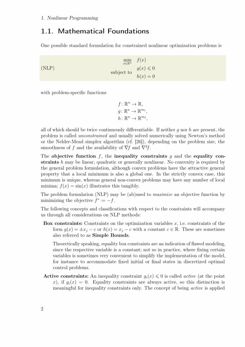
1.1. Mathematical Foundations
One possible standard formulation for constrained nonlinear optimization problems is
minx∈Rn
f(x)
subject tog(x) 6 0
h(x) = 0
(NLP)
with problem-speciőc functions
f : Rn → R,
g : Rn → Rm1 ,
h : Rn → Rm2 ,
all of which should be twice continuously diferentiable. If neither g nor h are present, theproblem is called unconstrained and usually solved numerically using Newton’s methodor the Nelder-Mead simplex algorithm (cf. [26]), depending on the problem size, thesmoothness of f and the availability of ∇f and ∇2f .
The objective function f , the inequality constraints g and the equality con-straints h may be linear, quadratic or generally nonlinear. No convexity is required bythe general problem formulation, although convex problems have the attractive generalproperty that a local minimum is also a global one. In the strictly convex case, thisminimum is unique, whereas general non-convex problems may have any number of localminima; f(x) = sin(x) illustrates this tangibly.
The problem formulation (NLP) may be (ab)used to maximize an objective function byminimizing the objective f ∗ ..= −f .
The following concepts and classiőcations with respect to the constraints will accompanyus through all considerations on NLP methods:
Box constraints: Constraints on the optimization variables x, i.e. constraints of theform g(x) = ±xj − c or h(x) = xj − c with a constant c ∈ R. These are sometimesalso referred to as Simple Bounds.
Theoretically speaking, equality box constraints are an indication of ŕawed modeling,since the respective variable is a constant; not so in practice, where őxing certainvariables is sometimes very convenient to simplify the implementation of the model,for instance to accommodate őxed initial or őnal states in discretized optimalcontrol problems.
Active constraints: An inequality constraint gi(x) 6 0 is called active (at the pointx), if gi(x) = 0. Equality constraints are always active, so this distinction ismeaningful for inequality constraints only. The concept of being active is applied
2
1.1. Mathematical Foundations
to box constraints in complete analogy; to diferentiate, one may refer to them asactive box constraints.
It is sometimes convenient to deőne the Active Set I as the index set of all activeconstraints, like I(x) ..=
i ∈ {1, . . . ,m1}
gi(x) is active
.
Inactive constraints: An inequality constraint gi(x) 6 0 is called inactive (at thepoint x), if gi(x) < 0, or equivalently, if it is not active.
Feasible set: The feasible set is deőned as the set of all points x, where both inequalityand equality constraints are satisőed, i.e. the set
{x ∈ Rn | g(x) 6 0 and h(x) = 0}.
The feasible set may also be empty, in which case problem (NLP) is, for all intentsand purposes, ill-posed.
The NLP problem class encompasses various other classes of optimization problems, forinstance quadratic problems of the form
minx∈Rn
12xTQx+ rTx
subject toAx 6 b
Cx = d
with matrices Q,A and C and vectors b, c, d and r of appropriate dimensions. Thequadratic problem is convex if Q > 0; we will see later that this case is of great relevanceto SQP methods, because their concept is to locally approximate (NLP) by quadraticproblems with (essentially) Q > 0, since solutions to this problem are unique (in thestrictly convex case) and eicient numerical methods to őnd them are known.
Lagrange Function & Multipliers
Constrained optimization relies heavily on the Lagrange function, which is deőned interms of (NLP) as
L(x, λ, µ) := f(x) + λTg(x) + µTh(x),
where λ ∈ Rm1 and µ ∈ Rm2 , are called the Lagrange multipliers (or dual variables śthe optimization variables x are referred to as primal variables in this context). Othersources deőne L with diferent signs, or impose inequality constraints as g(x) > 0;these conventions result in various subsequent sign changes, but luckily all conceivablepermutations of signs yield equivalent formulations of the same problemÐwith theexception of f , where a sign change turns minimization into maximization problems andvice versa.
The dual variables are often underappreciated, since the primal variables are at the centerof interest to the underlying optimization problem, and instances where the multipliershold a tangible meaning are uncommon; economic models are a notable exception to
3
1. Nonlinear Programming
this rule: Here the multipliers are referred to as accounting prices or opportunity costs,since they represent lost beneőts due to constraints. Results from parametric sensitivityanalysis[10, 11] generalize this widely known fact, asserting that the Lagrange multipliersin a local optimum describe the sensitivity of the optimal objective function value toperturbations of the corresponding constraint.
More precisely: Suppose we replace gi(x) 6 0 in (NLP) by gi(x) 6 ε and solve theperturbed problem to obtain the optimal solution x⋆
ε. If gi is active at x⋆ε and additional
smoothness and regularity assumptions hold, then
f(x⋆ε) = f(x⋆
0)− λi · ε+ o
ε2
for łsuiciently smallž ε,
i.e. in terms of sensitivity diferentials λi = −∂f∂ε(x⋆
0).
Conditions for optimal solutions
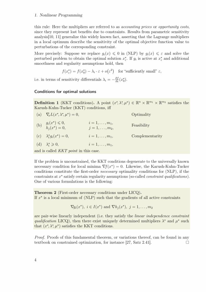
Definition 1 (KKT conditions). A point (x⋆, λ⋆, µ⋆) ∈ Rn × Rm1 × Rm2 satisőes theKarush-Kuhn-Tucker (KKT) conditions, if
(a) ∇xL(x⋆, λ⋆, µ⋆) = 0, Optimality
(b)gi(x
⋆) 6 0, i = 1, . . . ,m1, Feasibilityhj(x
⋆) = 0, j = 1, . . . ,m2,
(c) λ⋆i gi(x
⋆) = 0, i = 1, . . . ,m1, Complementarity
(d) λ⋆i > 0, i = 1, . . . ,m1,
and is called KKT point in this case.
If the problem is unconstrained, the KKT conditions degenerate to the universally knownnecessary condition for local minima ∇f(x⋆) = 0. Likewise, the Karush-Kuhn-Tuckerconditions constitute the őrst-order necessary optimality conditions for (NLP), if theconstraints at x⋆ satisfy certain regularity assumptions (so-called constraint qualifications).One of various formulations is the following:
Theorem 2 (First-order necessary conditions under LICQ).If x⋆ is a local minimum of (NLP) such that the gradients of all active constraints
∇gi(x⋆), i ∈ I(x⋆) and ∇hj(x⋆), j = 1, . . . ,m2
are pair-wise linearly independent (i.e. they satisfy the linear independence constraintqualification LICQ), then there exist uniquely determined multipliers λ⋆ and µ⋆ suchthat (x⋆, λ⋆, µ⋆) satisőes the KKT conditions.
Proof. Proofs of this fundamental theorem, or variations thereof, can be found in anytextbook on constrained optimization, for instance [27, Satz 2.41].
4
1.1. Mathematical Foundations
Similar assertions can be made under weaker assumptions, involving bundles of directionscalled tangential cones, but the LICQ are among the most concise and intuitive ones. Itis the central statement of Theorem 2 which justiőes that NLP methods are designed toőnd KKT points.
For sufficient optimality conditions, we can again őnd inspiration in the unconstrainedcase, where the Hessian matrix ∇2f(x⋆) has to be positive deőnite, i.e. dT∇2f(x⋆)d > 0for all d = 0; this essentially translates to the constrained case, where the subspace ofłdirectionsž on which the Hessian matrix ∇2
xxL has to be positive deőnite are furtherqualiőed:
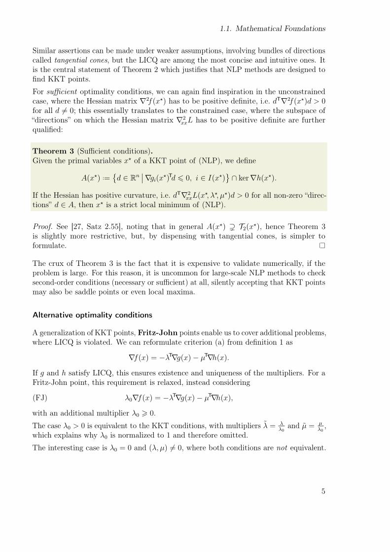
Theorem 3 (Suicient conditions).Given the primal variables x⋆ of a KKT point of (NLP), we deőne
A(x⋆) ..=
d ∈ Rn
∇gi(x⋆)Td 6 0, i ∈ I(x⋆)
∩ ker∇h(x⋆).
If the Hessian has positive curvature, i.e. dT∇2xxL(x
⋆, λ⋆, µ⋆)d > 0 for all non-zero łdirec-tionsž d ∈ A, then x⋆ is a strict local minimum of (NLP).
Proof. See [27, Satz 2.55], noting that in general A(x⋆) ) T2(x⋆), hence Theorem 3is slightly more restrictive, but, by dispensing with tangential cones, is simpler toformulate.
The crux of Theorem 3 is the fact that it is expensive to validate numerically, if theproblem is large. For this reason, it is uncommon for large-scale NLP methods to checksecond-order conditions (necessary or suicient) at all, silently accepting that KKT pointsmay also be saddle points or even local maxima.
Alternative optimality conditions
A generalization of KKT points, Fritz-John points enable us to cover additional problems,where LICQ is violated. We can reformulate criterion (a) from deőnition 1 as
∇f(x) = −λT∇g(x)− µT∇h(x).
If g and h satisfy LICQ, this ensures existence and uniqueness of the multipliers. For aFritz-John point, this requirement is relaxed, instead considering
(FJ) λ0∇f(x) = −λT∇g(x)− µT∇h(x),
with an additional multiplier λ0 > 0.
The case λ0 > 0 is equivalent to the KKT conditions, with multipliers λ = λλ0
and µ = µλ0
,which explains why λ0 is normalized to 1 and therefore omitted.
The interesting case is λ0 = 0 and (λ, µ) = 0, where both conditions are not equivalent.
5
1. Nonlinear Programming
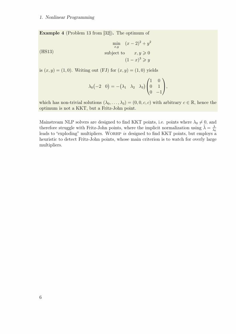
Example 4 (Problem 13 from [32]). The optimum of
minx,y
(x− 2)2 + y2
subject to x, y > 0
(1− x)3 > y
(HS13)
is (x, y) = (1, 0). Writing out (FJ) for (x, y) = (1, 0) yields
λ0
−2 0
= −
λ1 λ2 λ3
1 00 10 −1
,
which has non-trivial solutions (λ0, . . . , λ3) = (0, 0, c, c) with arbitrary c ∈ R, hence theoptimum is not a KKT, but a Fritz-John point.
Mainstream NLP solvers are designed to őnd KKT points, i.e. points where λ0 = 0, andtherefore struggle with Fritz-John points, where the implicit normalization using λ = λ
λ0
leads to łexplodingž multipliers. Worhp is designed to őnd KKT points, but employs aheuristic to detect Fritz-John points, whose main criterion is to watch for overly largemultipliers.
6
1.2. Penalty and barrier methods
1.2. Penalty and barrier methods
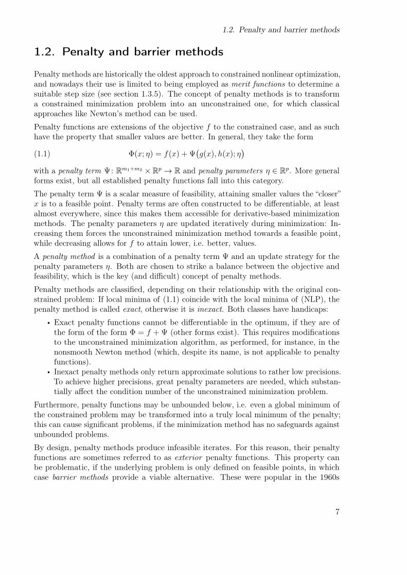
Penalty methods are historically the oldest approach to constrained nonlinear optimization,and nowadays their use is limited to being employed as merit functions to determine asuitable step size (see section 1.3.5). The concept of penalty methods is to transforma constrained minimization problem into an unconstrained one, for which classicalapproaches like Newton’s method can be used.
Penalty functions are extensions of the objective f to the constrained case, and as suchhave the property that smaller values are better. In general, they take the form
(1.1) Φ(x; η) = f(x) + Ψ
g(x), h(x); η
with a penalty term Ψ: Rm1+m2 ×Rp → R and penalty parameters η ∈ Rp. More generalforms exist, but all established penalty functions fall into this category.
The penalty term Ψ is a scalar measure of feasibility, attaining smaller values the łcloseržx is to a feasible point. Penalty terms are often constructed to be diferentiable, at leastalmost everywhere, since this makes them accessible for derivative-based minimizationmethods. The penalty parameters η are updated iteratively during minimization: In-creasing them forces the unconstrained minimization method towards a feasible point,while decreasing allows for f to attain lower, i.e. better, values.
A penalty method is a combination of a penalty term Ψ and an update strategy for thepenalty parameters η. Both are chosen to strike a balance between the objective andfeasibility, which is the key (and diicult) concept of penalty methods.
Penalty methods are classiőed, depending on their relationship with the original con-strained problem: If local minima of (1.1) coincide with the local minima of (NLP), thepenalty method is called exact, otherwise it is inexact. Both classes have handicaps:
• Exact penalty functions cannot be diferentiable in the optimum, if they are ofthe form of the form Φ = f +Ψ (other forms exist). This requires modiőcationsto the unconstrained minimization algorithm, as performed, for instance, in thenonsmooth Newton method (which, despite its name, is not applicable to penaltyfunctions).
• Inexact penalty methods only return approximate solutions to rather low precisions.To achieve higher precisions, great penalty parameters are needed, which substan-tially afect the condition number of the unconstrained minimization problem.
Furthermore, penalty functions may be unbounded below, i.e. even a global minimum ofthe constrained problem may be transformed into a truly local minimum of the penalty;this can cause signiőcant problems, if the minimization method has no safeguards againstunbounded problems.
By design, penalty methods produce infeasible iterates. For this reason, their penaltyfunctions are sometimes referred to as exterior penalty functions. This property canbe problematic, if the underlying problem is only deőned on feasible points, in whichcase barrier methods provide a viable alternative. These were popular in the 1960s
7
1. Nonlinear Programming
(cf. for instance [23] from 1955) but lost interest with the advent of newer methods likeSQP, which were regarded as more eicient. Shortly after Karmarkar published hispolynomial-complexity algorithm [42] for linear programming in 1984, its similarity tothe seemingly obsolete barrier methods was discovered, and they became a key elementof the interior-point methods (cf. the overview article [21] for an account).
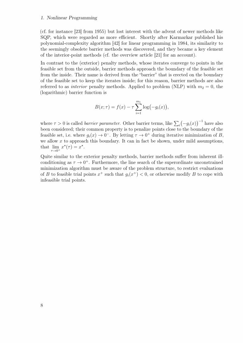
In contrast to the (exterior) penalty methods, whose iterates converge to points in thefeasible set from the outside, barrier methods approach the boundary of the feasible setfrom the inside. Their name is derived from the łbarrierž that is erected on the boundaryof the feasible set to keep the iterates inside; for this reason, barrier methods are alsoreferred to as interior penalty methods. Applied to problem (NLP) with m2 = 0, the(logarithmic) barrier function is
B(x; τ) = f(x)− τ
m1
i=1
log
−gi(x)
,
where τ > 0 is called barrier parameter. Other barrier terms, like
i
−gi(x)−1
have alsobeen considered; their common property is to penalize points close to the boundary of thefeasible set, i.e. where gi(x)→ 0−. By letting τ → 0+ during iterative minimization of B,we allow x to approach this boundary. It can in fact be shown, under mild assumptions,that lim
τ→0+x⋆(τ) = x⋆.
Quite similar to the exterior penalty methods, barrier methods sufer from inherent ill-conditioning as τ → 0+. Furthermore, the line search of the superordinate unconstrainedminimization algorithm must be aware of the problem structure, to restrict evaluationsof B to feasible trial points x+ such that gi(x+) < 0, or otherwise modify B to cope withinfeasible trial points.
8

1.3. Sequential Quadratic Programming
1.3. Sequential Quadratic Programming
Building on the concise theoretical foundations in section 1.1, this part introduces Se-quential Quadratic Programming as a prominent and successful method for the numericalsolution of (NLP).
SQP methods for general nonlinear problems were őrst considered as early as 1976 byHan [31], by generalizing results from the PhD thesis [76] of Wilson in 1963, who hadconsidered a special case. Despite their advanced age of 50 years, SQP methods arestill used widely, for instance in KNITRO (to solve barrier problems), NPSOL, SNOPT,NLPQLP, or the MATLAB optimization toolboxÐand, of course, in Worhp, being theyoungest solver of the above enumeration. SQP uses derivatives to iteratively minimizelocal approximations of the nonlinear functions, a general principle shared by mostderivative-based descent methods for nonlinear problems, sketched in őgure 1.1.
Checktermination
criteria
Computesearch
direction
Determinestep size
Updatederivatives
Initialguess
Solution
Figure 1.1.: General principle of derivative-based minimization algorithms: The choiceand computation of the search direction is the linchpin of every method.
Computing the Search Direction
The fundamental idea of SQP is to őnd KKT points by applying Newton’s method,giving it good (local) convergence properties, but entail the use of second derivatives: Tomotivate the approach, őrst consider (NLP) without inequality constraints g, leaving uswith the equality-constrained, nonlinear problem
minx∈Rn
f(x)
subject to h(x) = 0.(NLPeq)
9
1. Nonlinear Programming
Its KKT points can very concisely be characterized as points (x, µ) that satisfy thenonlinear equation
Φ(x, µ) =
∇xL(x, µ)h(x)
= 0
Assuming that both f and h are twice continuously diferentiable, we can apply Newton’smethod to derive the iteration scheme
(x[k+1], µ[k+1]) = (x[k], µ[k])− Φ′(x[k], µ[k])−1Φ(x[k], µ[k]).
By setting (∆x,∆µ) ..= (x[k+1]−x[k], µ[k+1]−µ[k]), we can rearrange the Newton iterationabove to an iterative solution of the linear equation system
Φ′(x, µ)
∆x
∆µ
= −Φ(x, µ).
We can spell this out, using Φ′ =
∇2xxL ∇hT∇h 0
, to result in
∇2xxL(x, µ)∆x+∇h(x)T∆µ = −∇xL(x, µ)
∇h(x)∆x = −h(x),
which we can simplify by deőning new multipliers µ+ ..= µ+∆µ to
∇2xxL(x, µ)∆x+∇h(x)Tµ+ = −∇f(x)
∇h(x)∆x = −h(x).(KKTeq)
Applying some łreverse engineeringž, we notice that (KKTeq) are the KKT conditions ofthe equality-constrained quadratic problem
min∆x∈Rn
12∆xT∇2
xxL(x, µ)∆x+∇f(x)T∆x
subject to h(x) +∇h(x)∆x = 0,(QPeq)
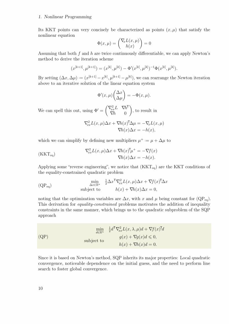
noting that the optimization variables are ∆x, with x and µ being constant for (QPeq).This derivation for equality-constrained problems motivates the addition of inequalityconstraints in the same manner, which brings us to the quadratic subproblem of the SQPapproach
mind∈Rn
12dT∇2
xxL(x, λ, µ)d+∇f(x)Td
subject tog(x) +∇g(x)d 6 0,
h(x) +∇h(x)d = 0.
(QP)
Since it is based on Newton’s method, SQP inherits its major properties: Local quadraticconvergence, noticeable dependence on the initial guess, and the need to perform linesearch to foster global convergence.
10
1.3. Sequential Quadratic Programming
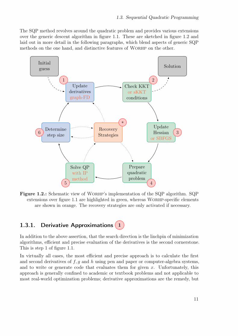
The SQP method revolves around the quadratic problem and provides various extensionsover the generic descent algorithm in őgure 1.1. These are sketched in őgure 1.2 andlaid out in more detail in the following paragraphs, which blend aspects of generic SQPmethods on the one hand, and distinctive features of Worhp on the other.
Check KKTor sKKTconditions
UpdateHessian
or SBFGS
Preparequadraticproblem
Updatederivativesgraph-FD
Determinestep size
Solve QPwith IPmethod
Initialguess Solution
RecoveryStrategies
1 2
3
45
6
∗
Figure 1.2.: Schematic view of Worhp’s implementation of the SQP algorithm. SQPextensions over őgure 1.1 are highlighted in green, whereas Worhp-speciőc elements
are shown in orange. The recovery strategies are only activated if necessary.
1.3.1. Derivative Approximations 1
In addition to the above assertion, that the search direction is the linchpin of minimizationalgorithms, eicient and precise evaluation of the derivatives is the second cornerstone.This is step 1 of őgure 1.1.
In virtually all cases, the most eicient and precise approach is to calculate the őrstand second derivatives of f, g and h using pen and paper or computer-algebra systems,and to write or generate code that evaluates them for given x. Unfortunately, thisapproach is generally conőned to academic or textbook problems and not applicable tomost real-world optimization problems; derivative approximations are the remedy, but
11
1. Nonlinear Programming
need further reőnement before they become usable, since Worhp is designed as a sparseNLP solver, suitable for sparse high-dimensional optimization problems with thousandsor millions of variables and constraints.
Definition 5 (Sparsity). A matrix A = (aij) ∈ Rm×n is called sparse, if aij = 0 forłmanyž pairs (i, j).
Applied to a diferentiable function f = (f1, . . . , fm) : Rn → Rm, sparsity is the structural
property of its Jacobian matrix ∇f that
(∇f)ij =∂fi
∂xj
≡ 0
for łmanyž pairs (i, j). These entries are called structural zeros, whereas those entries,where the derivative does not vanish everywhere, are called nonzero entries. Notethat both properties only depend on the structure of f , not on the point, where ∇f isevaluated; as such, nonzero entries may well attain 0 as numerical value. The number ofnonzero entries is commonly denoted as nnz.
The term sparsity is also used to describe the ratio nnz
n·m∈ (0, 1]. Matrices or derivatives
with sparsity 1 are called dense, whereas ratios close to 0 are called (very) sparse.
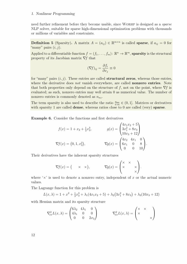
Example 6. Consider the functions and őrst derivatives
f(x) = 1 + x2 +13x33, g(x) =
4x1x2 + 53x2
1 + 8x3
10x3 + 12
∇f(x) =
0, 1, x23
, ∇g(x) =
4x2 4x1 06x1 0 80 0 10
.
Their derivatives have the inherent sparsity structures
∇f(x) =
× ×
, ∇g(x) =
× ×× ×
×
.
where ‘×’ is used to denote a nonzero entry, independent of x or the actual numericvalues.
The Lagrange function for this problem is
L(x, λ) = 1 + x2 + 13x33 + λ1(4x1x2 + 5) + λ2
3x21 + 8x3
+ λ3(10x3 + 12)
with Hessian matrix and its sparsity structure
∇2xxL(x, λ) =
6λ2 4λ1 04λ1 0 00 0 2x3
∇2xxL(x, λ) =
× ××
×
12
1.3. Sequential Quadratic Programming
Finite differences
Derivatives of any order can be approximated by the universally known őnite diference(FD) approach, although its inherent ill-conditioning, together with őnite precisionarithmetic imposes tight limits on achievable derivative order and precision.
To compute derivatives, Worhp has a őnite diference module that employs the standardmethods
(first-order) forward / backward differences
∂f
∂xi
(x) =f(x± h · ei)− f(x)
h+ o(|h|),
and (first-order) central differences
∂f
∂xi
(x) =f(x+ h · ei)− f(x− h · ei)
2h+ o
h2
to compute őrst (partial) derivatives, and also second (partial) derivatives using, forinstance, second-order forward differences
∂2f
∂xi∂xj
(x) =f
x+ h · (ei + ej)
− f(x+ h · ei)− f(x+ h · ej) + f(x)
h2+ o(h)
Gill, Murray and Wright [29] give a more extensive account on FD approximations, alongwith considerations on the optimal choice of the perturbation h as compromise betweencut-of and cancellation error.
Coming back to Worhp’s design for solving large-scale sparse problems, techniques forcomputing FD approximations with tolerable efort are crucial. The technique for ∇f isobvious: Only calculate FD approximations for its nonzero entries, cutting the requiredevaluations of f from n to nnz 6 n, assuming that the unperturbed value f(x) is cached.
Computing FD approximations for ∇g, however (and in complete analogy ∇h, which wewill omit here), is not as simple, since the general case is that g depends on most, ifnot all variables xj. If we can evaluate g component-wise, i.e. gi(x), we are in the samecase as with ∇f . Unfortunately, this case is the exception, and g is usually evaluated asłblack-boxž, vector-valued function.
The solution is to group the variables xj according to the dependency of the components gion them: Two variables xj and xk can be paired, if each component gi depends on at mostone of them. Applying this approach to all variables, we can construct 1 6 ng 6 n groups,each of which contains one or more variables. The case ng = n may indicate that one gi
13
1. Nonlinear Programming
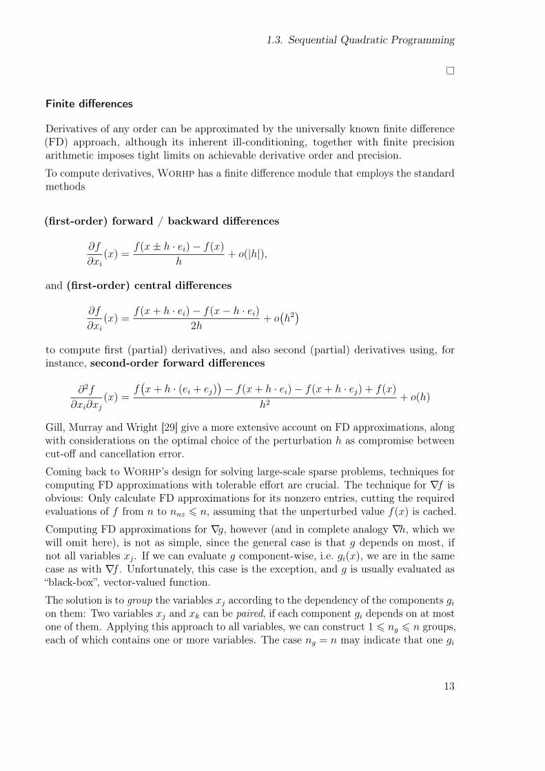
∇g =
×× × × ×
××
(a) g2 thwarts grouping, ng = n
∇g =
××
××
(b) Just one group ng = 1
∇g =
×× ×× ×× ×
(c) Grouping with ng = 2
Figure 1.3.: Three examples for variable grouping; per-column coloring indicates thevariable groups.
depends on all xj , whereas the (uncommon) case ng = 1 implies, that the components gidepend on pair-wise diferent variables xj, for instance if ∇g has a (permuted) diagonalsparsity structure. Three graphical examples in őgure 1.3 illustrate the concept.
This variable grouping is of practical relevance for our purposes, since it allows toreduce the number of evaluations of g for computing a forward (or backward) diferenceapproximation of ∇g from n to ng:
Consider example 1.3 (c), where perturbing x1 by evaluating g(x+ h · e1) only afects g1and g2, whereas gi(x+ h · e1) = gi(x) for i = 3, 4; vice versa, if we perturb x3. Thus wecan aggregate (x1, x3) and (x2, x4), evaluate
g
x+ h(e1 + e3)
and g
x+ h(e2 + e4)
,
and compute the appropriate diferences to calculate forward diferences. This approachonly requires 2 evaluations, where the naive one needs 4; as alluded above, it is nocoincidence that 2 = ng; the construction principle of the groups allows to aggregatethe perturbations for all variables in the group, thus reducing the number of evaluationsfrom n to ng.
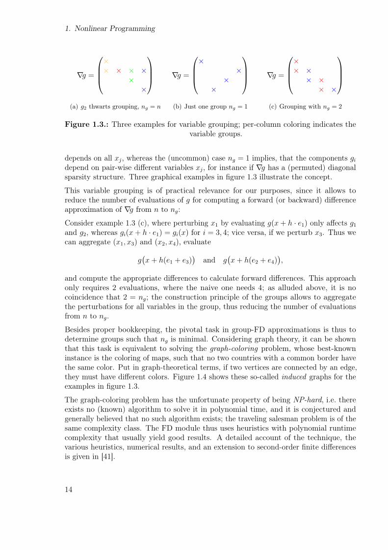
Besides proper bookkeeping, the pivotal task in group-FD approximations is thus todetermine groups such that ng is minimal. Considering graph theory, it can be shownthat this task is equivalent to solving the graph-coloring problem, whose best-knowninstance is the coloring of maps, such that no two countries with a common border havethe same color. Put in graph-theoretical terms, if two vertices are connected by an edge,they must have diferent colors. Figure 1.4 shows these so-called induced graphs for theexamples in őgure 1.3.
The graph-coloring problem has the unfortunate property of being NP-hard, i.e. thereexists no (known) algorithm to solve it in polynomial time, and it is conjectured andgenerally believed that no such algorithm exists; the traveling salesman problem is of thesame complexity class. The FD module thus uses heuristics with polynomial runtimecomplexity that usually yield good results. A detailed account of the technique, thevarious heuristics, numerical results, and an extension to second-order őnite diferencesis given in [41].
14
1.3. Sequential Quadratic Programming
x1 x2
x3 x4
(a) Graph for 1.3 (a)
x1 x2
x3 x4
(b) Graph for 1.3 (b)
x1 x2
x3 x4
(c) Graph for 1.3 (c)
Figure 1.4.: Induced graphs for the examples in őgure 1.3. The graphs are constructedby connecting two variables xk and xj, if there exists a gi that depends on both.
The group-FD technique is of particular value to Worhp, because the full discretizationor collocation approaches for discretizing optimal control problems typically result inhigh-dimensional, but very sparse and regularly structured matrices. The groupingapproach can be highly eicient for this class of problems, and the (optimal) number ofrequired groups is independent of the grid, a property we call discretization-invariance.
Dense BFGS update
To motivate the BFGS update, a small detour to the one-dimensional case is in order.Newton’s method for a given diferentiable function f : R→ R is
xk+1 = xk −f(xk)
f ′(xk),
and has local convergence order 2, if f ′ is Lipschitz continuous. Its drawback, however,is that it requires knowledge of the derivative and two function evaluations per iteration.The secant method
xk+1 = xk −xk − xk−1
f(xk)− f(xk−1)· f(xk)
on the other hand has a lower convergence order of 12(1 +
√5) ≈ 1.618, but only requires
one function evaluation per iteration, if f(xk−1) is cached. This leads to the secantmethod often being faster, despite its lower convergence order, and even if f and f ′ arestill moderately cheap to evaluate; the speed advantage increases, as evaluations of fand f ′ get more expensive.
Back to SQP methods: The derivation with Newton’s method leads to (QP), whichrequires second derivatives ∇2
xxL(x, λ, µ). With the same motivation as in the one-dimensional case, we could try and replace this derivative by an extension of the se-cant method to the multi-dimensional case. Independently of each other, Broyden[9],Fletcher[20], Goldfarb[30], and Shanno[64] followed this path and devised the BFGSupdate in 1970. The alternative name quasi-Newton method(s) seems to have beencoined by Shanno.
15
1. Nonlinear Programming
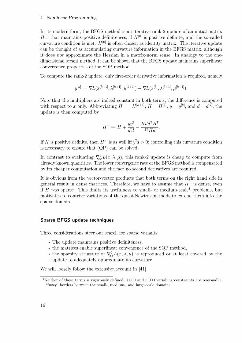
In its modern form, the BFGS method is an iterative rank-2 update of an initial matrixH [0] that maintains positive deőniteness, if H [0] is positive deőnite, and the so-calledcurvature condition is met. H [0] is often chosen as identity matrix. The iterative updatecan be thought of as accumulating curvature information in the BFGS matrix, althoughit does not approximate the Hessian in a matrix-norm sense. In analogy to the one-dimensional secant method, it can be shown that the BFGS update maintains superlinearconvergence properties of the SQP method.
To compute the rank-2 update, only őrst-order derivative information is required, namely
y[k] ..= ∇L(x[k+1], λ[k+1], µ[k+1])−∇L(x[k], λ[k+1], µ[k+1]).
Note that the multipliers are indeed constant in both terms, the diference is computedwith respect to x only. Abbreviating H+ = H [k+1], H = H [k], y = y[k], and d = d[k], theupdate is then computed by
H+ ..= H +yyT
yTd− HddTHT
dTHd.
If H is positive deőnite, then H+ is as well if yTd > 0; controlling this curvature conditionis necessary to ensure that (QP) can be solved.
In contrast to evaluating ∇2xxL(x, λ, µ), this rank-2 update is cheap to compute from
already known quantities. The lower convergence rate of the BFGS method is compensatedby its cheaper computation and the fact no second derivatives are required.
It is obvious from the vector-vector products that both terms on the right hand side ingeneral result in dense matrices. Therefore, we have to assume that H+ is dense, evenif H was sparse. This limits its usefulness to small- or medium-scale1 problems, butmotivates to contrive variations of the quasi-Newton methods to extend them into thesparse domain.
Sparse BFGS update techniques
Three considerations steer our search for sparse variants:
• The update maintains positive deőniteness,• the matrices enable superlinear convergence of the SQP method,• the sparsity structure of ∇2
xxL(x, λ, µ) is reproduced or at least covered by theupdate to adequately approximate its curvature.
We will loosely follow the extensive account in [41].
1Neither of these terms is rigorously defined; 1,000 and 5,000 variables/constraints are reasonable,“fuzzy” borders between the small-, medium-, and large-scale domains.
16
1.3. Sequential Quadratic Programming
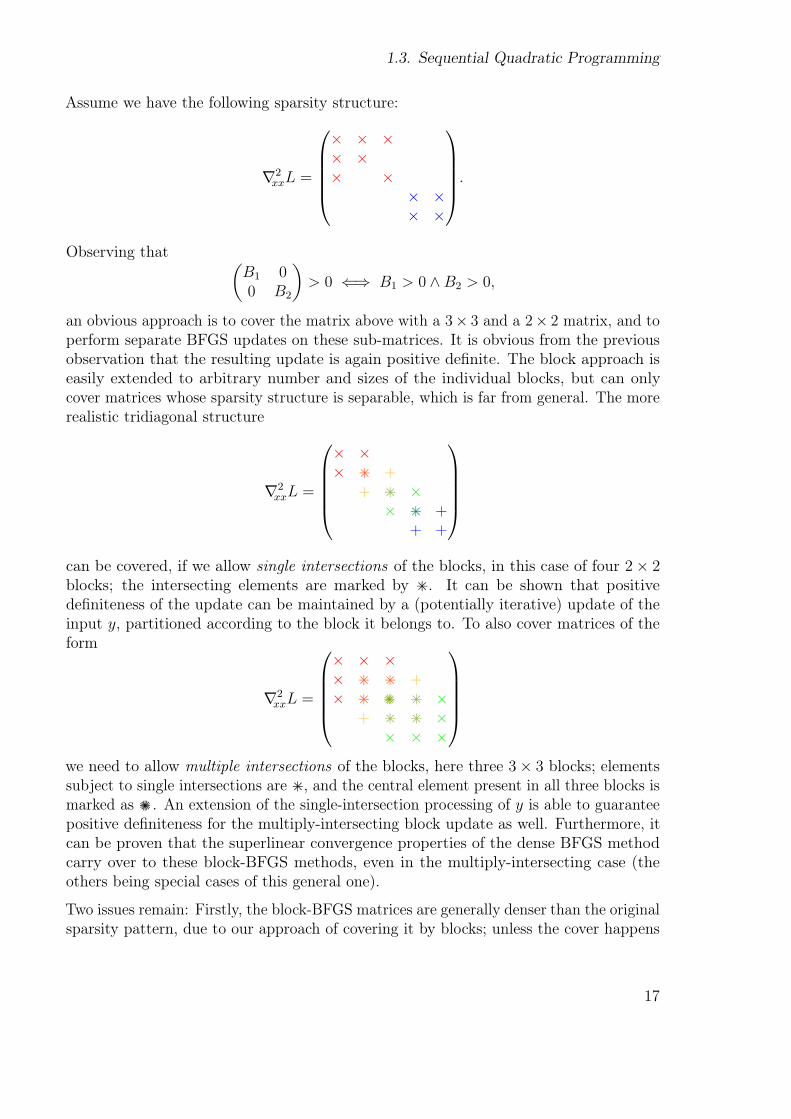
Assume we have the following sparsity structure:
∇2xxL =
× × ×× ×× ×
× ×× ×
.
Observing that
B1 00 B2
> 0 ⇐⇒ B1 > 0 ∧ B2 > 0,
an obvious approach is to cover the matrix above with a 3× 3 and a 2× 2 matrix, and toperform separate BFGS updates on these sub-matrices. It is obvious from the previousobservation that the resulting update is again positive deőnite. The block approach iseasily extended to arbitrary number and sizes of the individual blocks, but can onlycover matrices whose sparsity structure is separable, which is far from general. The morerealistic tridiagonal structure
∇2xxL =
× ×× ×+ +
+ ×+ ×× ×+ +
+ +
can be covered, if we allow single intersections of the blocks, in this case of four 2× 2blocks; the intersecting elements are marked by ×+. It can be shown that positivedeőniteness of the update can be maintained by a (potentially iterative) update of theinput y, partitioned according to the block it belongs to. To also cover matrices of theform
∇2xxL =
× × ×× ×+ ×+ +× ×+ ×+×+ ×+ ×
+ ×+ ×+ ×× × ×
we need to allow multiple intersections of the blocks, here three 3× 3 blocks; elementssubject to single intersections are ×+, and the central element present in all three blocks ismarked as ×+×+. An extension of the single-intersection processing of y is able to guaranteepositive deőniteness for the multiply-intersecting block update as well. Furthermore, itcan be proven that the superlinear convergence properties of the dense BFGS methodcarry over to these block-BFGS methods, even in the multiply-intersecting case (theothers being special cases of this general one).
Two issues remain: Firstly, the block-BFGS matrices are generally denser than the originalsparsity pattern, due to our approach of covering it by blocks; unless the cover happens
17
1. Nonlinear Programming
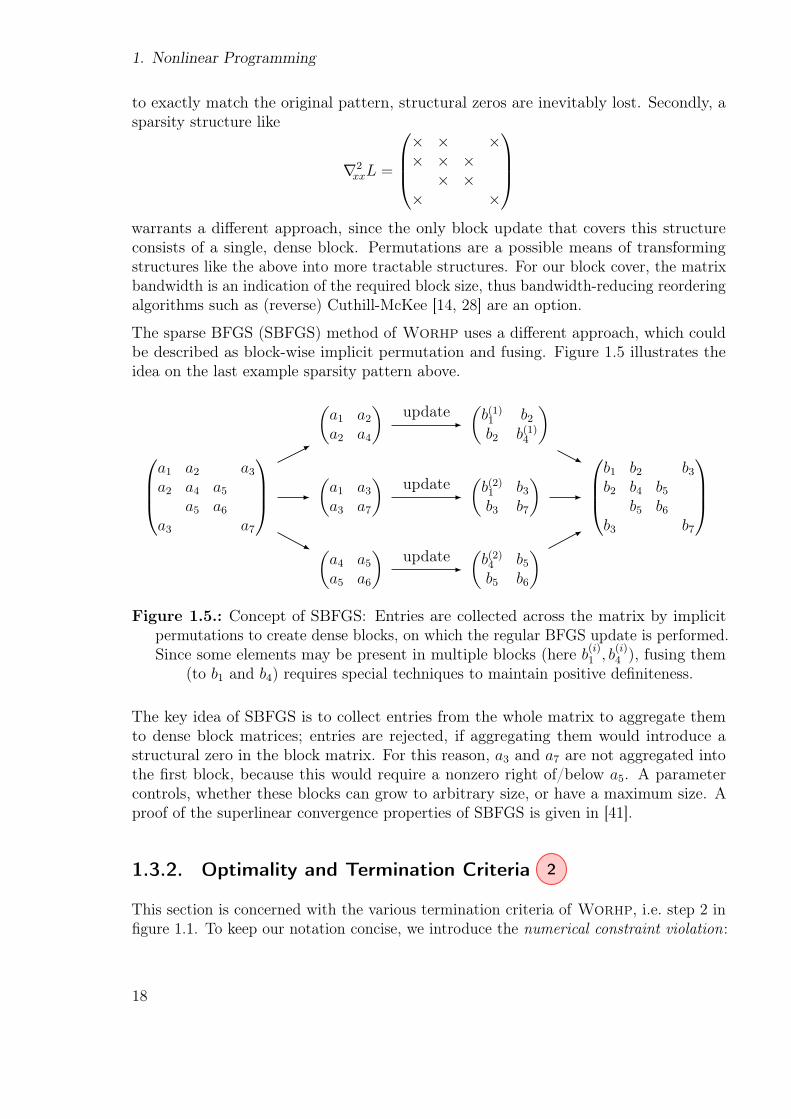
to exactly match the original pattern, structural zeros are inevitably lost. Secondly, asparsity structure like
∇2xxL =
× × ×× × ×× ×
× ×
warrants a diferent approach, since the only block update that covers this structureconsists of a single, dense block. Permutations are a possible means of transformingstructures like the above into more tractable structures. For our block cover, the matrixbandwidth is an indication of the required block size, thus bandwidth-reducing reorderingalgorithms such as (reverse) Cuthill-McKee [14, 28] are an option.
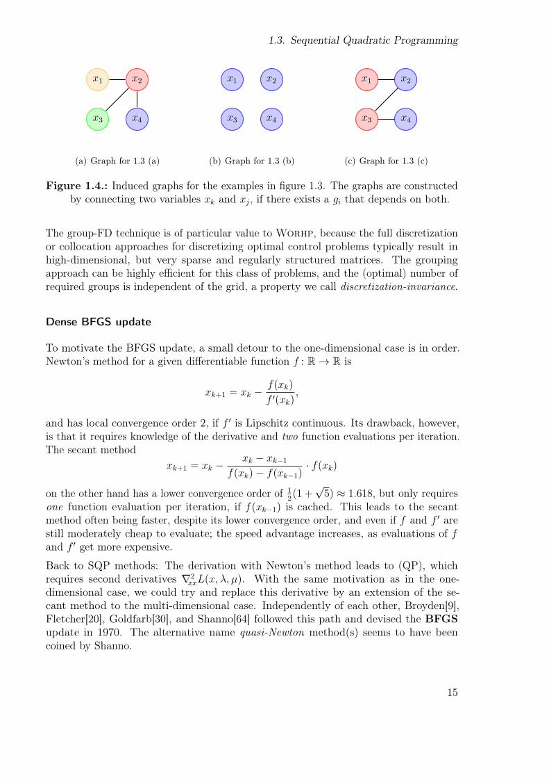
The sparse BFGS (SBFGS) method of Worhp uses a diferent approach, which couldbe described as block-wise implicit permutation and fusing. Figure 1.5 illustrates theidea on the last example sparsity pattern above.
a1 a2 a3a2 a4 a5
a5 a6a3 a7
a1 a2a2 a4
a1 a3a3 a7
a4 a5a5 a6
b(1)1 b2b2 b(1)4
b(2)1 b3b3 b7
b(2)4 b5b5 b6
b1 b2 b3b2 b4 b5
b5 b6b3 b7
update
update
update
Figure 1.5.: Concept of SBFGS: Entries are collected across the matrix by implicitpermutations to create dense blocks, on which the regular BFGS update is performed.Since some elements may be present in multiple blocks (here b
(i)1 , b
(i)4 ), fusing them
(to b1 and b4) requires special techniques to maintain positive deőniteness.
The key idea of SBFGS is to collect entries from the whole matrix to aggregate themto dense block matrices; entries are rejected, if aggregating them would introduce astructural zero in the block matrix. For this reason, a3 and a7 are not aggregated intothe őrst block, because this would require a nonzero right of/below a5. A parametercontrols, whether these blocks can grow to arbitrary size, or have a maximum size. Aproof of the superlinear convergence properties of SBFGS is given in [41].
1.3.2. Optimality and Termination Criteria 2
This section is concerned with the various termination criteria of Worhp, i.e. step 2 inőgure 1.1. To keep our notation concise, we introduce the numerical constraint violation:
18
1.3. Sequential Quadratic Programming
Definition 7. The numerical constraint violation c is a scalar quantity that allowsto gauge quantitatively, how well a point x satisőes the constraints of the standardoptimization problem (NLP):
c(x) ..=max(i,j)
max
0, gi(x)
,
hj(x)
for all (i, j) ∈ {1, . . . ,m1} × {1, . . . ,m2}(CV)
In the strict sense, x is feasible if c(x) = 0.
Scaled KKT conditions
Due to their design, the KKT conditions are the canonical termination criterion for SQPmethods; despite their diferent design, this is also true for the Interior-Point methods.Adapted to the realities of őnite precision arithmetic, and given a triplet of small, positivetolerances εopti, εfeas, and εcomp, the standard KKT conditions impose
(a) ∥∇xL(x, λ, µ)∥ 6 εopti, Optimality
(b) c(x) 6 εfeas Feasibility
(c) λigi(x) 6 εcomp, i = 1, . . . ,m1, Complementarity
(d) λi > 0, i = 1, . . . ,m1,
where ∥ · ∥ can be any norm, but usually ∥ · ∥p with p ∈ {1, 2,∞}.Unfortunately, the standard KKT conditions are not robust against numerical error;criterion (a) is particularly sensitive against small perturbations of the derivatives, suchas the error incurred from őnite-diference approximations. Due to Worhp’s approachfor solving the quadratic subproblems, the multipliers introduce further rounding errors:The QP-solver never returns multipliers that are exactly zero, even if the correspondingconstraint is inactive.
Criterion (b) causes the solver to struggle if the constraints are badly scaled, but it isa design decision of Worhp to not scale the constraints. This is not at least becausethere is no canonical way of scaling them, and because we do not want to łsoftenž thenotion of feasibility, as some other NLP solvers do2; a point that is feasible in Worhp’ssense is guaranteed to satisfy all constraints to the prescribed precision.
An inspiration for improving on the standard conditions ŕows from the users’ wish todetermine values of x that satisfy
|f(x⋆)− f(x)| 6 εopti.
2The elastic mode of SNOPT is a prime example: Troublesome constraints are removed from theproblem and instead added to the objective, using a penalty approach to (try and) satisfy them.
19
1. Nonlinear Programming
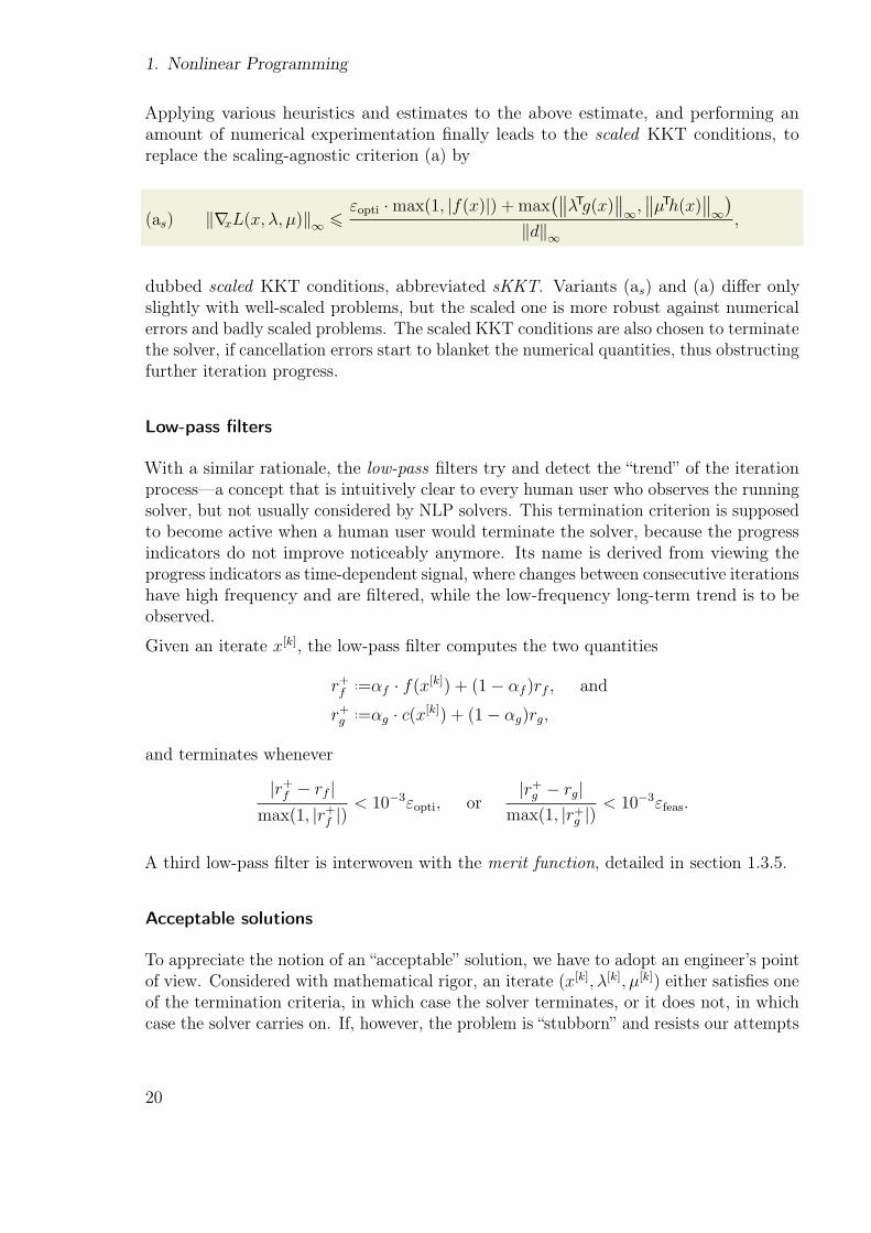
Applying various heuristics and estimates to the above estimate, and performing anamount of numerical experimentation őnally leads to the scaled KKT conditions, toreplace the scaling-agnostic criterion (a) by
(as) ∥∇xL(x, λ, µ)∥∞ 6εopti ·max(1, |f(x)|) + max
λTg(x)
∞,
µTh(x)
∞
∥d∥∞,
dubbed scaled KKT conditions, abbreviated sKKT. Variants (as) and (a) difer onlyslightly with well-scaled problems, but the scaled one is more robust against numericalerrors and badly scaled problems. The scaled KKT conditions are also chosen to terminatethe solver, if cancellation errors start to blanket the numerical quantities, thus obstructingfurther iteration progress.
Low-pass filters
With a similar rationale, the low-pass őlters try and detect the łtrendž of the iterationprocessÐa concept that is intuitively clear to every human user who observes the runningsolver, but not usually considered by NLP solvers. This termination criterion is supposedto become active when a human user would terminate the solver, because the progressindicators do not improve noticeably anymore. Its name is derived from viewing theprogress indicators as time-dependent signal, where changes between consecutive iterationshave high frequency and are őltered, while the low-frequency long-term trend is to beobserved.
Given an iterate x[k], the low-pass őlter computes the two quantities
r+f..=αf · f(x[k]) + (1− αf )rf , and
r+g..=αg · c(x[k]) + (1− αg)rg,
and terminates whenever
|r+f − rf |max(1, |r+f |)
< 10−3εopti, or|r+g − rg|
max(1, |r+g |)< 10−3εfeas.
A third low-pass őlter is interwoven with the merit function, detailed in section 1.3.5.
Acceptable solutions
To appreciate the notion of an łacceptablež solution, we have to adopt an engineer’s pointof view. Considered with mathematical rigor, an iterate (x[k], λ[k], µ[k]) either satisőes oneof the termination criteria, in which case the solver terminates, or it does not, in whichcase the solver carries on. If, however, the problem is łstubbornž and resists our attempts
20
1.3. Sequential Quadratic Programming
to őnd optimal points to high precision, or if solutions close to an optimal solution arehelpful for the user, returning acceptable solutions makes sense.
An iterate (x[k], λ[k], µ[k]) is considered acceptable, if it satisőes the (scaled) KKT conditionsto a lower precision; be default, Worhp uses εacc
◦..=√ε◦ instead of the strict tolerance ε◦,
for ◦ ∈ {opti, feas}, although this can be chosen by the user. Obviously, setting εacc◦ = ε◦
disables this behavior.
The notion is useful only, if the solver is forced to terminate before őnding a strictlyoptimal solution. This can be caused by
• reaching a user-deőned limit (maxiter, timeout),• slow progress,• an error condition in the model that cannot be alleviated, or• user intervention.
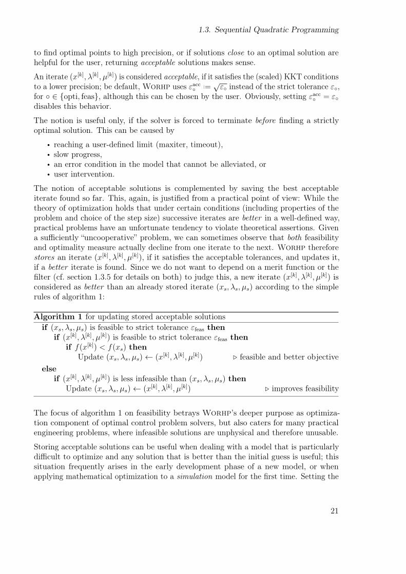
The notion of acceptable solutions is complemented by saving the best acceptableiterate found so far. This, again, is justiőed from a practical point of view: While thetheory of optimization holds that under certain conditions (including properties of theproblem and choice of the step size) successive iterates are better in a well-deőned way,practical problems have an unfortunate tendency to violate theoretical assertions. Givena suiciently łuncooperativež problem, we can sometimes observe that both feasibilityand optimality measure actually decline from one iterate to the next. Worhp thereforestores an iterate (x[k], λ[k], µ[k]), if it satisőes the acceptable tolerances, and updates it,if a better iterate is found. Since we do not want to depend on a merit function or theőlter (cf. section 1.3.5 for details on both) to judge this, a new iterate (x[k], λ[k], µ[k]) isconsidered as better than an already stored iterate (xs, λs, µs) according to the simplerules of algorithm 1:
Algorithm 1 for updating stored acceptable solutionsif (xs, λs, µs) is feasible to strict tolerance εfeas then
if (x[k], λ[k], µ[k]) is feasible to strict tolerance εfeas thenif f(x[k]) < f(xs) then
Update (xs, λs, µs)← (x[k], λ[k], µ[k]) ◃ feasible and better objective
elseif (x[k], λ[k], µ[k]) is less infeasible than (xs, λs, µs) then
Update (xs, λs, µs)← (x[k], λ[k], µ[k]) ◃ improves feasibility
The focus of algorithm 1 on feasibility betrays Worhp’s deeper purpose as optimiza-tion component of optimal control problem solvers, but also caters for many practicalengineering problems, where infeasible solutions are unphysical and therefore unusable.
Storing acceptable solutions can be useful when dealing with a model that is particularlydiicult to optimize and any solution that is better than the initial guess is useful; thissituation frequently arises in the early development phase of a new model, or whenapplying mathematical optimization to a simulation model for the őrst time. Setting the
21
1. Nonlinear Programming
acceptable tolerances to high absolute values instructs Worhp to start storing iteratesearly.
Additional heuristics
As mentioned earlier, many practical optimization problems have the unfortunate tendencyto disregard mathematical prerequisites, such as f, g and h being suiciently smooth,satisfying a constraint qualiőcation in the optimum, or for the whole problem to bebounded from below. Worhp’s heuristics can be considered as last-ditch efort to őndłgoodž solutions even in cases, where our theory and the numerical methods fail.
Most simple, the unbounded problem detection heuristic triggers, if the current iterate isfeasible, if the last search direction d[k] is a descent direction (i.e. ∇f(x[k])Td[k] < 0) andthe objective falls below a őxed limit, −1020 by default.
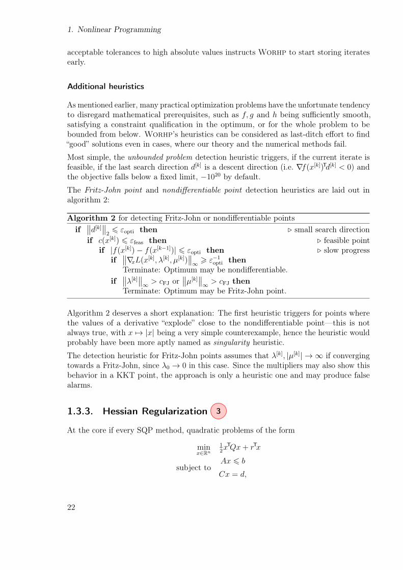
The Fritz-John point and nondifferentiable point detection heuristics are laid out inalgorithm 2:
Algorithm 2 for detecting Fritz-John or nondiferentiable pointsif
d[k]
26 εopti then ◃ small search direction
if c(x[k]) 6 εfeas then ◃ feasible pointif |f(x[k])− f(x[k−1])| 6 εopti then ◃ slow progress
if
∇xL(x[k], λ[k], µ[k])
∞> ε−1
opti thenTerminate: Optimum may be nondiferentiable.
if
λ[k]
∞> cFJ or
µ[k]
∞> cFJ then
Terminate: Optimum may be Fritz-John point.
Algorithm 2 deserves a short explanation: The őrst heuristic triggers for points wherethe values of a derivative łexplodež close to the nondiferentiable pointÐthis is notalways true, with x →→ |x| being a very simple counterexample, hence the heuristic wouldprobably have been more aptly named as singularity heuristic.
The detection heuristic for Fritz-John points assumes that λ[k], |µ[k]| → ∞ if convergingtowards a Fritz-John, since λ0 → 0 in this case. Since the multipliers may also show thisbehavior in a KKT point, the approach is only a heuristic one and may produce falsealarms.
1.3.3. Hessian Regularization 3
At the core if every SQP method, quadratic problems of the form
minx∈Rn
12xTQx+ rTx
subject toAx 6 b
Cx = d,
22
1.3. Sequential Quadratic Programming
have to be solved. For the solution to be well-deőned and unique, Q has to be positivedeőnite on the subspace spanned by the kernels of A and C, i.e.
xTQx > 0 for all x ∈ span{kerA, kerC},
otherwise we lose uniqueness, or the problem may be unbounded. One can guess thatensuring this numerically would require QR, singular value or Schur decompositions, allof which are too expensive in the large-scale case. A common approach is therefore toensure Q > 0 on the whole space, instead of the subspace dependent on A and C. If Qis a BFGS matrix, we remember that positive deőniteness is one of its most importantproperties. If, however, Q = ∇2
xxL, some work is in order:
To ensure positive deőniteness of Q without prohibitive computational costs, Levenberg-Marquadt regularization may be used. This is done by determining a lower bound onthe smallest eigenvalue of Q, the so-called Gerschgorin bound
σ = min16i6n
qii −n
j =i
|qij|
and using it to update Q by
(1.2) Q+ = Q+ τ ·max{−σ, 1}I.
Here I denotes the identity matrix and τ is a factor which is adapted iteratively: choosingτ = 1 guarantees positive deőniteness, since it shifts the spectrum such that it is boundedfrom below by 1, but the Hessian matrix may be perturbed drastically if the Gerschgorinbound produces a negative σ with great modulus, either because the smallest eigenvalueis negative with great modulus, or because the Gerschgorin estimate is bad. Due tothe inexact nature of the Gerschgorin estimate, τ = 1 is suicient but not necessary forestablishing positive deőniteness. The iterative update of Worhp tries to let τ [k] ↘ 0 asx[k] → x⋆, since ∇2
xxL can be shown to have the right spectral properties in a minimum(confer also theorem 3), hence no regularization is required in a neighborhood of x⋆.
1.3.4. Prepare the Quadratic Problem 4
Besides the regularization of the Hessian matrix, further modiőcations of the linear-quadratic problem approximation are either necessary or beneőcial. Constraint relaxationensures that the constraints can be satisőed, although they are only approximated toőrst order, while the weak-Active Set method was devised to use less memory andcomputational time by problem size reduction.
Constraint Relaxation
Problem (QP) may not always have a solution, which can be demonstrated by a verysimple example. This also serves to demonstrate one of the dangers of starting from a
23
1. Nonlinear Programming
trivial initial guess, such as x[0] = 0; the exact deőnition of what constitutes a trivialinitial guess depends, of course, on the optimization problem.
Example. Consider the nonlinear inequality constraint
g(x) = 1− x26 0.
Linearizing this constraint at x[0] = 0, we arrive at the inequality
g(x[0]) + g′(x[0]) · d = 1 + 0 · d 6 0,
which obviously cannot be satisőed, hence (QP) cannot be solved.
To work around the problem of unsolvable QPs, Powell introduced the idea to performa constraint relaxation (also referred to as elastic constraints) by introducing aconstraint relaxation variable δ ∈ [0, 1] and an associated constraint relaxation penaltyparameter ηr > 0, and using them to reformulate (QP) as
mind∈Rn, δ∈[0,1]
12dT∇2
xxL(x, λ, µ)d+∇f(x)Td+ ηr2δ2
subject to(1− σiδ)gi(x) +∇gi(x)d 6 0, i = 1, . . . ,m1
(1− δ)h(x) + ∇h(x)d = 0.
(rQP)
with
σi =
0, if gi(x) < 0, i.e. gi is inactive
1, otherwise
In practice, (rQP) is transformed into the standard QP formulation through
Qr =
∇2xxL 00 ηr
and minimizing over dr =
d
δ
.
The key advantage of constraint relaxation is that (d, δ) = (0, 1) is always feasible for(rQP). If, however, the solution (d, δ) satisőes δ = 0, it is optimal for (QP). Therelaxation variable can be controlled through the penalty term ηr: If it is too small,the resulting search direction d will not suiciently decrease the constraint violation,hence the SQP method cannot converge to a feasible point. If ηr is chosen too large, thecondition number of the extended matrix Qr is large and the QP-solver may fail, or yieldan imprecise solution. To őnd a compromise between both extremes, ηr is initially smalland iteratively increased if δ exceeds a given upper bound.
By default, Worhp uses a single relaxation variable for all constraints. One canalternatively choose to use m1 + m2 relaxation variables, i.e. one for each constraint,which increases the QP dimensions and computational time, but may increase stabilityand overall performance for problems with łdiicultž constraints.
24
1.3. Sequential Quadratic Programming
Weak-Active Set
The weak-Active Set method is inspired by the established Active Set method for solvinginequality-constrained quadratic problems. The concept of the (strict) Active Set methodis to identify the set I of active indices. The quadratic problem (QP) is then modiőed to
mind∈Rn
12dT∇2
xxL(x, λ, µ)d+∇f(x)Td
subject togi(x) +∇gi(x)d = 0, i ∈ I
h(x) +∇h(x)d = 0.
(QPAS)
i.e. the inactive inequality constraints are identiőed and dropped from the problem. Themanual pen-and-paper solution of optimization problems is very similar to this approach.
The modiőed problem is equality-constrained and can be solved without further ado bysolving a system of linear equations. The task of identifying the Active Set is nontrivial,however, because it may change between iterations (although it stabilizes when theSQP method converges to a solution), and because the solver essentially has to make aprediction for the active set at the next iterate x[k+1] that is computed using I(x[k+1]).Since g is nonlinear, the prediction can be inaccurate, hence an iterative update procedureis needed, with an exponential worst-case performance of O(2m1).
While Interior-Point methods do not sufer from this complication, introducing the slackvariables increases the problem size; this efect is strongest if the problem has manyinequalities, which is very pronounced in discretized optimal control problems with pathconstraints. To take advantage of the beneőts of both methods, the weak-Active Setmethod uses a conservative estimate to remove inequality constraints, and thus reducethe size of the quadratic subproblems (QP). This method does not share the diiculties ofits strict precursor, since the estimate of the active set may be fuzzy, and any łsuspiciousžinequality constraints can be left untouched, since there is no need to transform theminto equality constraints.
Definition (weak-Active Set). Let x ∈ Rn and δw ∈ R with δw > 0. A constraint gi(x)is called weak-active, when gi(x) 6 δw. Equality constraints are always weak-active. Theweak-Active Set Iw is given by Iw(x) =
i ∈ {1, . . . ,m1}
gi(x) is weak-active
.
Applying this deőnition to (QP) gives us
mind∈Rn
12dT∇2
xxL(x, λ, µ)d+∇f(x)Td
subject togi(x) +∇gi(x)d 6 0, i ∈ Iw(x)
h(x) +∇h(x)d = 0.
(QPwAS)
The key diference to (QPAS) is that the inequality constraints do not need to be łforcedžto equalities, since the QP-solver is able to handle them by using an Interior-Pointmethod, whereas older QP-solvers were only able to solve equality-constrained problems.
25
1. Nonlinear Programming
In contrast to the original method, the weak-Active Set technique is used to lower thecomputational efort, and not as a problem transformation required by the availablemethods.
1.3.5. Determine Step Size 6
Owing to its łheritagež as an application of Newton’s method, SQP methods have toperform line search to achieve global convergence as well. The task is to determine astep size α, usually α ∈ (0, 1], such that
x[k+1] ..= x[k] + αd[k]
satisőes some performance criterion. If the problem is unconstrained, as in Newton’smethod, this criterion is simply the objective f to be minimized. In constrained opti-mization, however, feasibility is an additional, usually conŕicting criterion to consider.Complementarity can be construed as yet another criterion, but is only considered in thetermination criteria of Worhp.
Assuming we have a scalar performance criterion Φ: Rn → R that behaves similar to f ,in that smaller values mean better performance, we can deőne the scalar function
(1.3) φ : R→ R, φ(α) ..= Φ
x[k] + αd[k]
,
Further assuming that Φ is smooth, so is φ, and this invites us to apply methods fromunconstrained, one-dimensional minimization, such as the secant or Newton’s method, todetermine
αmin = argminα∈(0,1]
φ(α).
However, considering that this line search is but a single step embedded in the iterativescheme of the whole minimization algorithm, and that Φ is potentially expensive toevaluateÐsince it will have to involve f , g, and hÐ, determining the exact minimumαmin is unnecessary efort.
Instead of performing (exact) line search, NLP methods in general perform variants ofinexact line search which test a (small) number of trial step sizes αi. Since the theoryholds that α = 1 is the optimal step size in a neighborhood of x⋆, α0 = 1 is generallyused as őrst trial step, with further steps deőned through
αi = βi, i = 1, . . . , imax
with a decrease factor β ∈ (0, 1) and an upper limit to the number of trial steps imax ∈ N.Worhp modiőes the choice of trial step sizes slightly, since for certain problem classes,α0 = 1 − ε seems to be beneőcial. Therefore, Worhp uses trial step sizes αi = α0β
i,
where α0 can be inŕuenced through a solver parameter.
Acceptance or rejection of a trial step size depends on the employed globalization method,where Worhp uses merit functions and a (2D-)filter as two major alternatives.
26
1.3. Sequential Quadratic Programming
Merit functions
The function Φ in equation (1.3) is called merit function, which is an equivalent conceptto the penalty functions shown in section 1.2. Worhp implements two merit functions:The Augmented Lagrangian
La(x, λ, µ; γ, η) = f(x) + 12
m1
i=1
1
γi
max{0, λi + γigi(x)}2 − λ2
i
+
m2
i=1
µihi(x) +12
m2
i=1
ηih2i (x)
(AL)
and the L1 merit function (also known as exact L1 penalty function)
(L1) L1(x; γ, η) = f(x) +
m1
i=1
γi max(0, gi(x)) +
m2
i=1
ηi|hi(x)|
.
The SQP algorithm is highly sensitive to the choice of the penalty parameters (γ, η), andtheir update is non-trivial. While the Augmented Lagrangian is diferentiable, the L1
merit function has nondiferentiable points. However, the L1 merit function does possessa directional derivative along the search direction, and thus φ(α) ..= Φ
x[k] + αd[k]
isdiferentiable for Φ = L1.
Given a merit function Φ and the function φ constructed from it, various strategies existto decide whether to accept or reject a trial step size αi, established ones being theArmijo(-Goldstein) rule and the Wolfe-Powell rule:
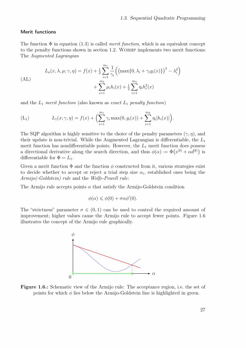
The Armijo rule accepts points α that satisfy the Armijo-Goldstein condition
φ(α) 6 φ(0) + σαφ′(0).
The łstrictnessž parameter σ ∈ (0, 1) can be used to control the required amount ofimprovement; higher values cause the Armijo rule to accept fewer points. Figure 1.6illustrates the concept of the Armijo rule graphically.
φ
α0
Figure 1.6.: Schematic view of the Armijo rule: The acceptance region, i.e. the set ofpoints for which φ lies below the Armijo-Goldstein line is highlighted in green.
27
1. Nonlinear Programming
Bounding the iterates from above guarantees a minimum amount of improvement,although not enough to make the Armijo rule efficient, which is a technical criterionused to proof the global convergence properties of SQP methods; it can be shown,however, that the scaled Armijo rule is eicient, if the trial step sizes are chosen asαi = sβi, i = 1, . . . , imax and s > 0 is chosen appropriately. However, the scaled variantprecludes the trial step size α = 1, which is required to łinheritž the quadratic convergenceorder from Newton’s method. Alternatively, choosing αi = β±i, i.e. interleaved increasingand decreasing trial step sizes also makes the Armijo rule eicient. In practice, Worhp
employs the standard Armijo-Goldstein condition to enable locally quadratic convergence,even though global convergence cannot be proven for this approach.
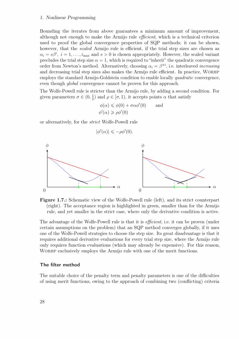
The Wolfe-Powell rule is stricter than the Armijo rule, by adding a second condition. Forgiven parameters σ ∈ (0, 1
2) and ρ ∈ [σ, 1), it accepts points α that satisfy
φ(α) 6 φ(0) + σαφ′(0) and
φ′(α) > ρφ′(0)
or alternatively, for the strict Wolfe-Powell rule
|φ′(α)| 6 −ρφ′(0).
φ
α0
φ
α0
Figure 1.7.: Schematic view of the Wolfe-Powell rule (left), and its strict counterpart(right). The acceptance region is highlighted in green, smaller than for the Armijorule, and yet smaller in the strict case, where only the derivative condition is active.
The advantage of the Wolfe-Powell rule is that it is efficient, i.e. it can be proven (undercertain assumptions on the problem) that an SQP method converges globally, if it usesone of the Wolfe-Powell strategies to choose the step size. Its great disadvantage is that itrequires additional derivative evaluations for every trial step size, where the Armijo ruleonly requires function evaluations (which may already be expensive). For this reason,Worhp exclusively employs the Armijo rule with one of the merit functions.
The filter method
The suitable choice of the penalty term and penalty parameters is one of the diicultiesof using merit functions, owing to the approach of combining two (conŕicting) criteria
28
1.3. Sequential Quadratic Programming
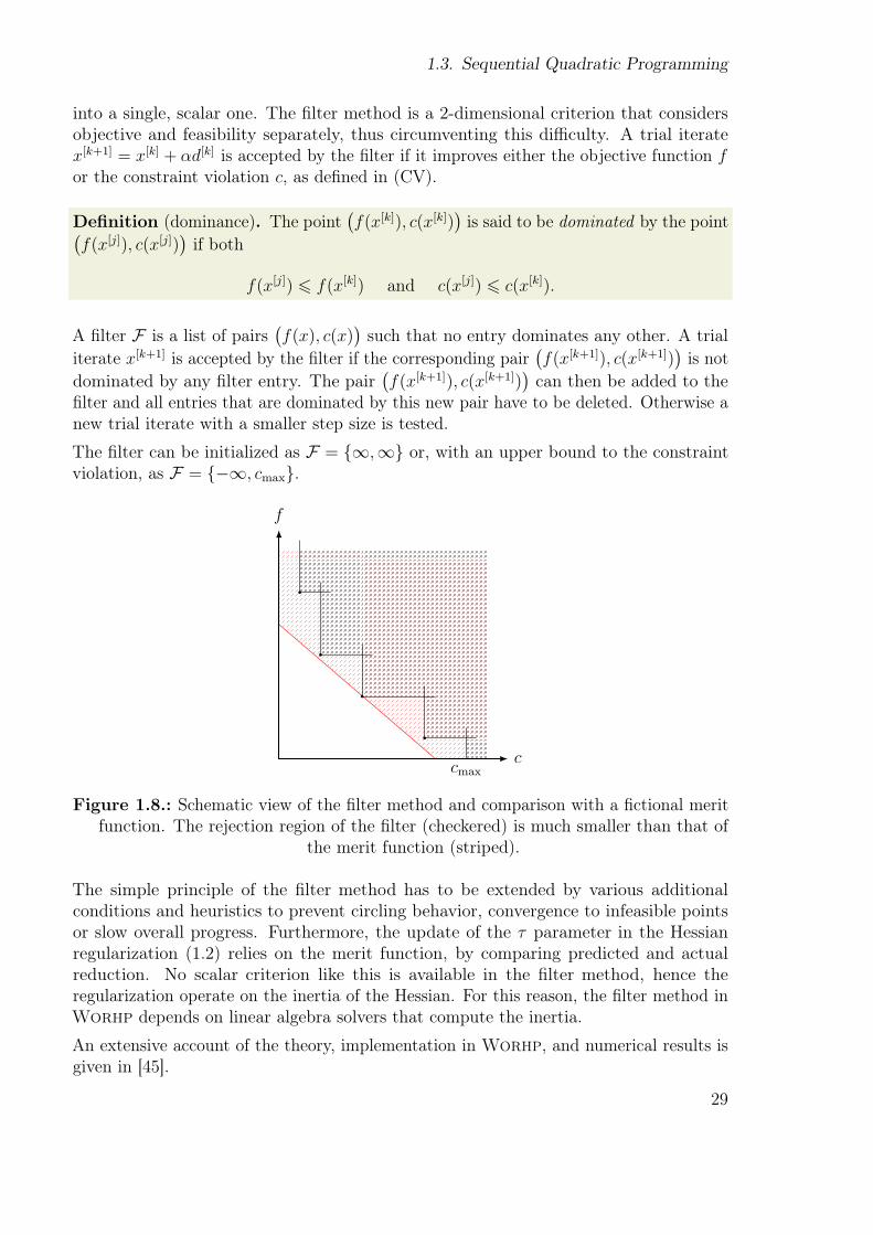
into a single, scalar one. The őlter method is a 2-dimensional criterion that considersobjective and feasibility separately, thus circumventing this diiculty. A trial iteratex[k+1] = x[k] + αd[k] is accepted by the őlter if it improves either the objective function f
or the constraint violation c, as deőned in (CV).
Definition (dominance). The point
f(x[k]), c(x[k])
is said to be dominated by the point
f(x[j]), c(x[j])
if both
f(x[j]) 6 f(x[k]) and c(x[j]) 6 c(x[k]).
A őlter F is a list of pairs
f(x), c(x)
such that no entry dominates any other. A trialiterate x[k+1] is accepted by the őlter if the corresponding pair
f(x[k+1]), c(x[k+1])
is notdominated by any őlter entry. The pair
f(x[k+1]), c(x[k+1])
can then be added to theőlter and all entries that are dominated by this new pair have to be deleted. Otherwise anew trial iterate with a smaller step size is tested.
The őlter can be initialized as F = {∞,∞} or, with an upper bound to the constraintviolation, as F = {−∞, cmax}.
cmax
f
c
Figure 1.8.: Schematic view of the őlter method and comparison with a őctional meritfunction. The rejection region of the őlter (checkered) is much smaller than that of
the merit function (striped).
The simple principle of the őlter method has to be extended by various additionalconditions and heuristics to prevent circling behavior, convergence to infeasible pointsor slow overall progress. Furthermore, the update of the τ parameter in the Hessianregularization (1.2) relies on the merit function, by comparing predicted and actualreduction. No scalar criterion like this is available in the őlter method, hence theregularization operate on the inertia of the Hessian. For this reason, the őlter method inWorhp depends on linear algebra solvers that compute the inertia.
An extensive account of the theory, implementation in Worhp, and numerical results isgiven in [45].
29

1. Nonlinear Programming
1.3.6. Recovery Strategies ∗
The line search is an obvious Achilles heel of the algorithm, since all previous stepsinŕuence its outcome; a bad initial guess, faulty derivatives, or an imprecise solutionof the QP. All of these inŕuences can cause a line search breakdown; unfortunately,backtracing the breakdown to its cause next to impossible, unless prohibitively expensiveanalysis tools constantly supervise the solver. The recovery strategies were devised ascheap(er) heuristics to be activated for a single iterations after a line search breakdownor an error condition in the QP solver.
Worhp has the following recovery strategies:
• The SLP (Successive Linear Programming) strategy replaces the Hessian or BFGSmatrix in (QP) by the identity, which essentially reduces the SQP method to aőrst-order steepest descent method. The rationale is that Q may have a highcondition number, which either causes a breakdown of the QP or linear solver, orlater in the line search, due to an inexact search direction. Replacing Q by thewell-conditioned identity eliminates this source of error.
• The non-monotone strategy allows local increase of the merit function, by replacingthe current value of the merit function Φ(x[k]) by its lowpass-őltered value, whichis always greater.
• The dual feasibility strategy activates the so-called dual feasibility mode which triesto őnd a feasible point by solving the least-squares problem min∥c(x)∥22. In őlterand Interior-Point methods, this step is called feasibility restoration. The term dualstems from the solution method: The QP solver internally solves linear systems ofthe form
Q AT
A 0
x
λ
=
f
c
,
which can be used to solve the normal equation ATAd = −ATc by rewriting it as
I A
AT 0
l
d
=
0−ATc
.
This is akin to the dual problem, hence the designation as dual feasibility mode.• As a last resort, the force strategy can be interpreted as a restart of the optimization
run. It forces the line search to accept the step size αf determined such that
αfd[k]
= 1 to make a suiciently great step to escape the current problematicregion.
Two further strategies, the ascent and the cut strategy, are heuristics that can charitablybe described as experimental and are better left undocumented.
30
Chapter2
Architecture of Worhp
A spider conducts operations that resemble those of a weaver,and a bee puts to shame many an architect in theconstruction of her cells. But what distinguishes the worstarchitect from the best of bees is this, that the architectraises his structure in imagination before he erects it in reality.
(Karl Marx, Das Kapital)
2.1. Practical Problem Formulation . . . . . . . . . . . . . . . . . . . . 33
2.2. Sparse Matrices . . . . . . . . . . . . . . . . . . . . . . . . . . . 35
2.2.1. Coordinate Storage format . . . . . . . . . . . . . . . . . . 35
2.2.2. Compressed Column format . . . . . . . . . . . . . . . . . 36
2.3. Data Housekeeping . . . . . . . . . . . . . . . . . . . . . . . . . . 38
2.3.1. The traditional many arguments convention . . . . . . . . 39
2.3.2. The USI approach in Worhp . . . . . . . . . . . . . . . . 40
2.4. Reverse Communication . . . . . . . . . . . . . . . . . . . . . . . 43
2.4.1. Division into stages . . . . . . . . . . . . . . . . . . . . . 44
2.4.2. Implementation considerations . . . . . . . . . . . . . . . . 46
2.4.3. Applications . . . . . . . . . . . . . . . . . . . . . . . . . 48
2.5. Serialization . . . . . . . . . . . . . . . . . . . . . . . . . . . . . 49
2.5.1. Hotstart functionality . . . . . . . . . . . . . . . . . . . . 49
2.5.2. Reading parameters . . . . . . . . . . . . . . . . . . . . . 49
2.5.3. Serialization format . . . . . . . . . . . . . . . . . . . . . 50
31

2. Architecture of WORHP
The architecture of Worhp was designed to overcome technical shortcomings of tradi-tional mathematical software architectures, to permit a high degree of user interactionwith the solver, to allow a higher degree of modularity than traditional mathematicalsoftware does and to enable both industrial-grade usability and its use as an academicexperimental platform.
The term łtraditional mathematical softwarež very loosely refers to many established andmature software packages written in some FORTRAN (i.e. pre-90) dialect, which oftenexcel in terms of performance or precision, but face diiculties regarding usability ormaintainability due to the remarkable restrictions of the language; from an architecturalpoint of view, Worhp is an attempt to right some of the wrongs imposed on programmersduring the long reign of the old FORTRAN standards and dialects.
The tools developed for and used in Worhp to this end are the Uniőed Solver Interface(USI) that deőnes a simple, yet powerful interfacing convention both externally andinternally, and together with the Reverse Communication (RC) paradigm allows anunprecedented degree of interaction with a piece of mathematical software, and incombination with the XML module ofers interesting possibilities for inspection, analysisand result processing. The őnal major tool of the bunch is Worhp’s workspace andmemory management, the weak spot of many FORTRAN software packages’ usability.
32
2.1. Practical Problem Formulation
2.1. Practical Problem Formulation
The standard formulation for constrained nonlinear optimization problems considered inchapter 1 is
minx∈Rn
f(x)
subject tog(x) 6 0
h(x) = 0,
(NLP)
which is very suitable and convenient for the theoretical considerations. However, itcan be cumbersome to formulate practical optimization problems, for instance a boxconstraint 1 6 xi 6 2. This is unfortunate for various reasons:
• It places an additional burden on the users, who have to reformulate their op-timization problems to match the abstract mathematical notation. This can beparticularly irksome, if the solver is integrated into existing models.
• In the case of box constraints, information is lost by transforming them into thestandard inequality formulation; box constraints receive special treatment in variousplaces, which improves both performance and stability.
• During development and integration, it may be useful to łswitchž individual con-straints on and of, or soften equality constraints to (tight) inequalities.
Therefore, Worhp operates on problems in the more ŕexible formulation
minx∈Rn
F (x)
subject to
l
L
6
x
G(x)
6
u
U
(OP)
with boundsl, u ∈ Rn and L,U ∈ Rm
and functionsF : Rn → R and G : Rn → Rm.
Formulations (NLP) and (OP) are equivalent through transformations of the form
g(x) = ±xi + c 6 0 ⇐⇒ c = li 6 xi or xi 6 ui = −c,g1(x) = −c(x) + c1 6 0g2(x) = c(x) + c2 6 0
⇐⇒ G(x) = c(x) and L = c1, U = −c2,
h(x) = c(x)− c = 0 ⇐⇒ G(x) = c(x) and L = U = c.
Since f is not afected by these transformations, we can always choose F ≡ f and neednot diferentiate further between both. The constraints G, on the other hand, and theirdimension m depend on the functions g and h, and on their dimensions m1 and m2 in anon-trivial way; only m > m2 holds in general, irrespective of the problem structure.
33
2. Architecture of WORHP
Note on multipliers
Unlike the convention for the mathematical formulation (NLP), Worhp uses multipliersλ for box constraints and µ for the general (G) constraints. In case of two-sided constraints,two (NLP)-multipliers are associated with a single constraint, but it only has a single(OP)-multiplier. This is only seemingly problematic: For equality constraints, both (NLP)-multipliers coincide, thus the (OP)-multiplier takes their common value; for inequalityconstraints, at most one of them can be active at any point, and the (OP)-multiplierattains the value of the active (NLP)-multiplier, the inactive one being silently discarded.
34
2.2. Sparse Matrices
2.2. Sparse Matrices
Due to its fundamental design as a solver for large-scale problems, Worhp operatesexclusively on sparse matrices (but can be łtrickedž into operating on dense matrices). Aslaid out in deőnition 5 and illustrated by example 6, the central idea behind sparse matrixrepresentations is the omission of zero entries, which saves memory and computationaltime. Nonzero entries deőne the sparse matrix structure, which is inherent to everyinstance of (NLP) and constant, while the actual values of the nonzero entries depend onthe current point (note that nonzero entries may of course attain the numeric value 0).
Worhp accepts two diferent sparse matrix representations: the Coordinate Storage (CS)format, or the Compressed Column (CC) format. They difer in their storage requirementsand their suitability for certain matrix operations. Both formats in general, and Worhp’sspecializations of them, are described in the following paragraphs. Worhp’s conventionsfor sparse matrix representation allow it to naturally operate on dense matrices given inFortran’s storage sequence for 2D arrays, without conversions or special indexing; onlythe Hessian matrix with its łdiagonal-lastž ordering is an exception to that rule.
2.2.1. Coordinate Storage format
The coordinate storage or triplet format is the łintuitivež sparse matrix format, where anonzero matrix entry a = (A)ij corresponds to an (a, i, j) triplet. These triplets are splitup into the val, row and col arrays such that (valk, rowk, colk) = (a, i, j)k for someenumeration k = 1, . . . , nnz of the nonzero entries; a priori, no kind of ordering has to beassumed for this construction. Thus the storage requirement for the CS format is nnz
double + 2nnz integer.
Since Worhp uses the CS format internally, it is the preferred sparse matrix format.
While the general format makes no assumptions on the sorting or uniqueness of theentries, Worhp imposes the following restrictions:
CS-1. Entries are sorted ascending in column-major order.
CS-2. Each matrix entry may be present at most once.
CS-3. Vectors only: The column index is omitted for sparse vectors.
CS-4. Hessian only: Only the lower triangular part is saved; őrst the strictly lowertriangular (i.e. subdiagonal) entries hij with i > j in column-major order, lastall diagonal entries hii in ascending order, regardless of whether the problemhas a nonzero entry at hii.
Restriction CS-1 is of special importance, because it allows the use of more eicientalgorithms, simpliőes conversion between CS and CC, and since its memory layoutcoincides with that of dense matrices in Fortran, Worhp can easily be integratedinto dense problem formulations. Restriction CS-4 is necessary to enable the Hessianregularization by diagonal update, described in section 1.3.3.
35
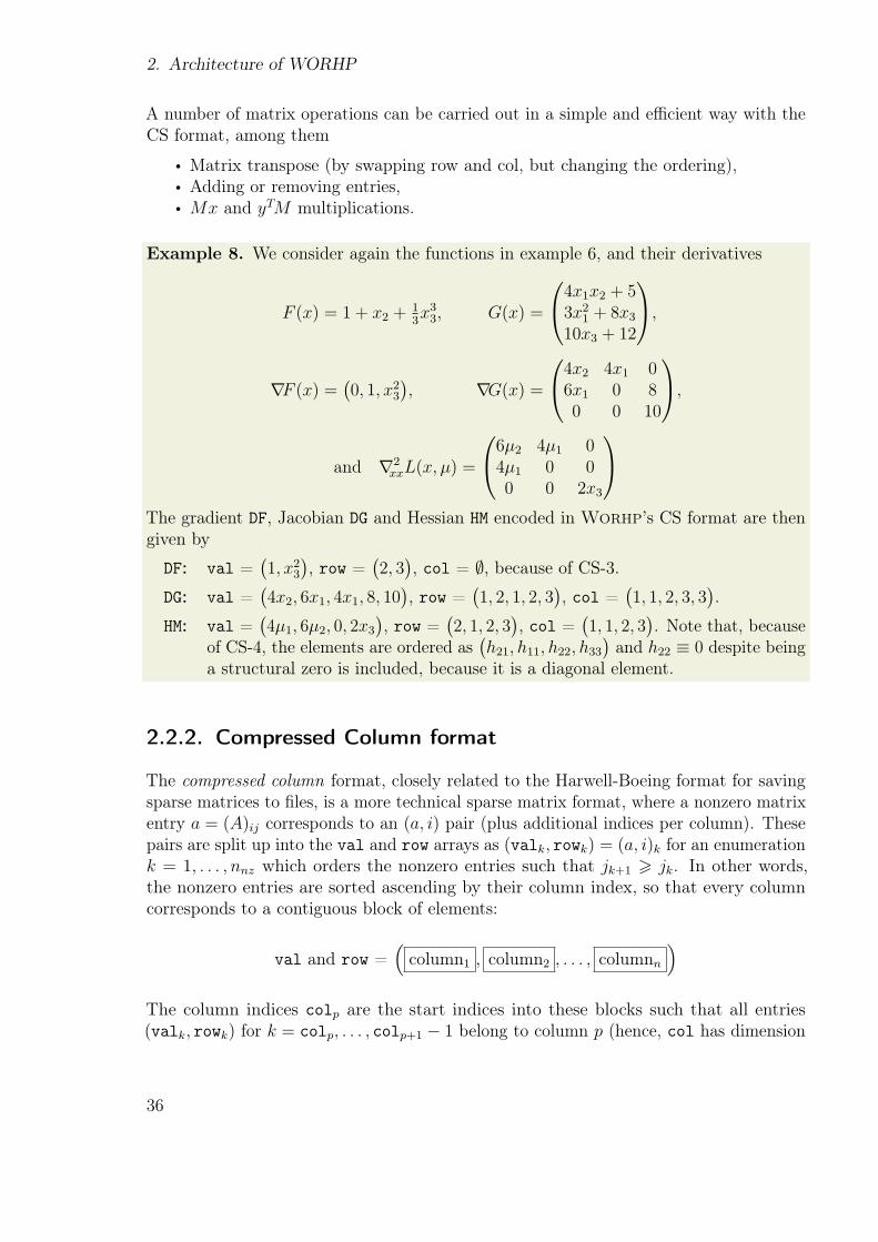
2. Architecture of WORHP
A number of matrix operations can be carried out in a simple and eicient way with theCS format, among them
• Matrix transpose (by swapping row and col, but changing the ordering),• Adding or removing entries,• Mx and yTM multiplications.
Example 8. We consider again the functions in example 6, and their derivatives
F (x) = 1 + x2 +13x33, G(x) =
4x1x2 + 53x2
1 + 8x3
10x3 + 12
,
∇F (x) =
0, 1, x23
, ∇G(x) =
4x2 4x1 06x1 0 80 0 10
,
and ∇2xxL(x, µ) =
6µ2 4µ1 04µ1 0 00 0 2x3
The gradient DF, Jacobian DG and Hessian HM encoded in Worhp’s CS format are thengiven by
DF: val =
1, x23
, row =
2, 3
, col = ∅, because of CS-3.
DG: val =
4x2, 6x1, 4x1, 8, 10
, row =
1, 2, 1, 2, 3
, col =
1, 1, 2, 3, 3
.
HM: val =
4µ1, 6µ2, 0, 2x3
, row =
2, 1, 2, 3
, col =
1, 1, 2, 3
. Note that, becauseof CS-4, the elements are ordered as
h21, h11, h22, h33
and h22 ≡ 0 despite beinga structural zero is included, because it is a diagonal element.
2.2.2. Compressed Column format
The compressed column format, closely related to the Harwell-Boeing format for savingsparse matrices to őles, is a more technical sparse matrix format, where a nonzero matrixentry a = (A)ij corresponds to an (a, i) pair (plus additional indices per column). Thesepairs are split up into the val and row arrays as (valk, rowk) = (a, i)k for an enumerationk = 1, . . . , nnz which orders the nonzero entries such that jk+1 > jk. In other words,the nonzero entries are sorted ascending by their column index, so that every columncorresponds to a contiguous block of elements:
val and row =
column1 , column2 , . . . , columnn
The column indices colp are the start indices into these blocks such that all entries(valk, rowk) for k = colp, . . . , colp+1 − 1 belong to column p (hence, col has dimension
36
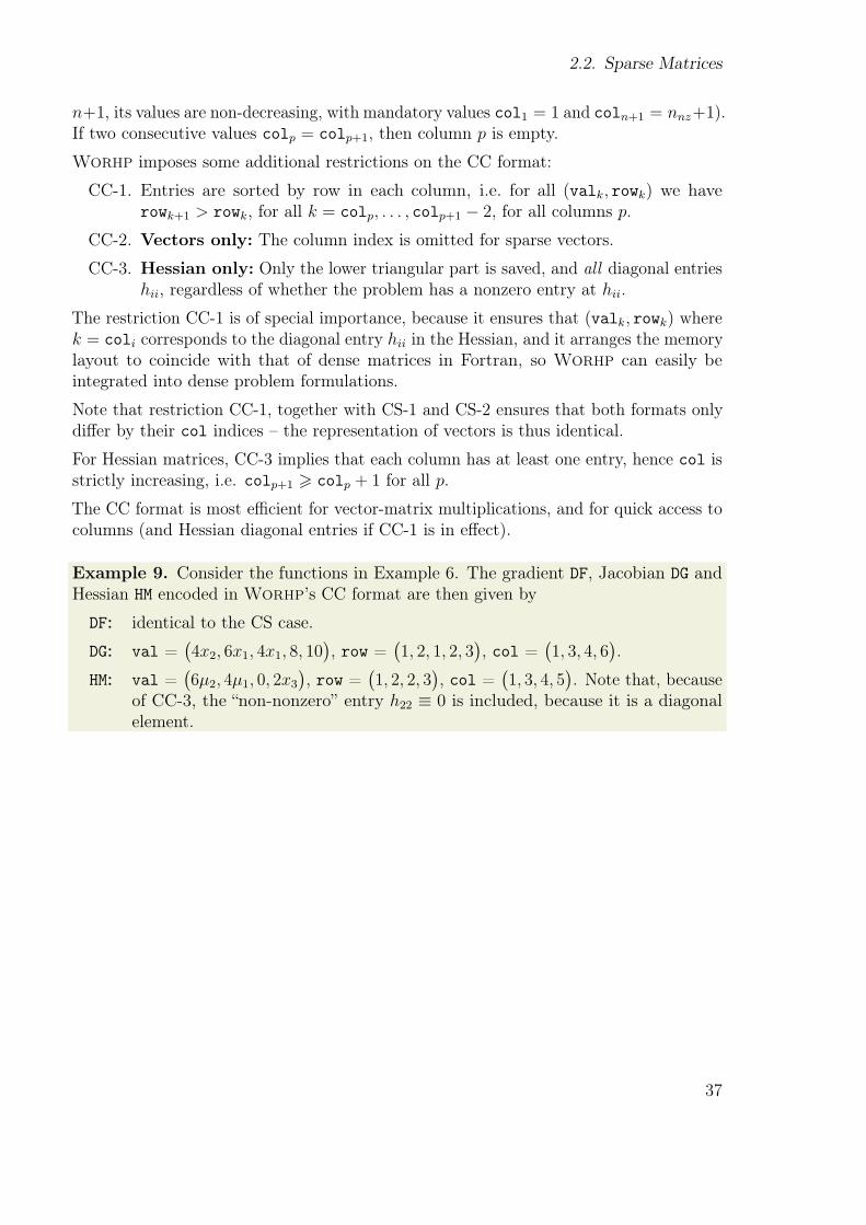
2.2. Sparse Matrices
n+1, its values are non-decreasing, with mandatory values col1 = 1 and coln+1 = nnz+1).If two consecutive values colp = colp+1, then column p is empty.
Worhp imposes some additional restrictions on the CC format:
CC-1. Entries are sorted by row in each column, i.e. for all (valk, rowk) we haverowk+1 > rowk, for all k = colp, . . . , colp+1 − 2, for all columns p.
CC-2. Vectors only: The column index is omitted for sparse vectors.
CC-3. Hessian only: Only the lower triangular part is saved, and all diagonal entrieshii, regardless of whether the problem has a nonzero entry at hii.
The restriction CC-1 is of special importance, because it ensures that (valk, rowk) wherek = coli corresponds to the diagonal entry hii in the Hessian, and it arranges the memorylayout to coincide with that of dense matrices in Fortran, so Worhp can easily beintegrated into dense problem formulations.
Note that restriction CC-1, together with CS-1 and CS-2 ensures that both formats onlydifer by their col indices ś the representation of vectors is thus identical.
For Hessian matrices, CC-3 implies that each column has at least one entry, hence col isstrictly increasing, i.e. colp+1 > colp + 1 for all p.
The CC format is most eicient for vector-matrix multiplications, and for quick access tocolumns (and Hessian diagonal entries if CC-1 is in efect).
Example 9. Consider the functions in Example 6. The gradient DF, Jacobian DG andHessian HM encoded in Worhp’s CC format are then given by
DF: identical to the CS case.
DG: val =
4x2, 6x1, 4x1, 8, 10
, row =
1, 2, 1, 2, 3
, col =
1, 3, 4, 6
.
HM: val =
6µ2, 4µ1, 0, 2x3
, row =
1, 2, 2, 3
, col =
1, 3, 4, 5
. Note that, becauseof CC-3, the łnon-nonzerož entry h22 ≡ 0 is included, because it is a diagonalelement.
37
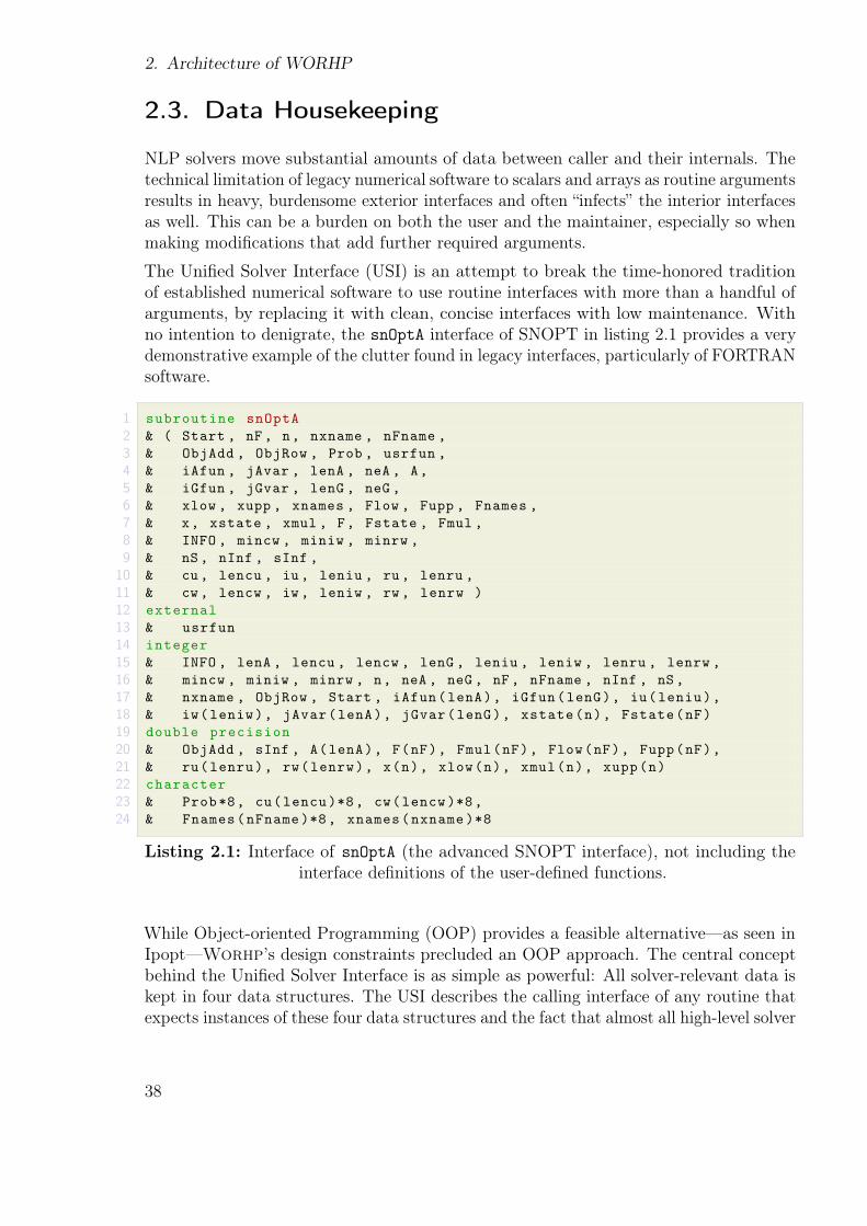
2. Architecture of WORHP
2.3. Data Housekeeping
NLP solvers move substantial amounts of data between caller and their internals. Thetechnical limitation of legacy numerical software to scalars and arrays as routine argumentsresults in heavy, burdensome exterior interfaces and often łinfectsž the interior interfacesas well. This can be a burden on both the user and the maintainer, especially so whenmaking modiőcations that add further required arguments.
The Uniőed Solver Interface (USI) is an attempt to break the time-honored traditionof established numerical software to use routine interfaces with more than a handful ofarguments, by replacing it with clean, concise interfaces with low maintenance. Withno intention to denigrate, the snOptA interface of SNOPT in listing 2.1 provides a verydemonstrative example of the clutter found in legacy interfaces, particularly of FORTRANsoftware.
1 subroutine snOptA
2 & ( Start , nF, n, nxname , nFname ,
3 & ObjAdd , ObjRow , Prob , usrfun ,
4 & iAfun , jAvar , lenA , neA , A,
5 & iGfun , jGvar , lenG , neG ,
6 & xlow , xupp , xnames , Flow , Fupp , Fnames ,
7 & x, xstate , xmul , F, Fstate , Fmul ,
8 & INFO , mincw , miniw , minrw ,
9 & nS, nInf , sInf ,
10 & cu, lencu , iu , leniu , ru, lenru ,
11 & cw, lencw , iw , leniw , rw, lenrw )
12 external
13 & usrfun
14 integer
15 & INFO , lenA , lencu , lencw , lenG , leniu , leniw , lenru , lenrw ,
16 & mincw , miniw , minrw , n, neA , neG , nF, nFname , nInf , nS,
17 & nxname , ObjRow , Start , iAfun(lenA), iGfun(lenG), iu(leniu),
18 & iw(leniw), jAvar(lenA), jGvar(lenG), xstate(n), Fstate(nF)
19 double precision
20 & ObjAdd , sInf , A(lenA), F(nF), Fmul(nF), Flow(nF), Fupp(nF),
21 & ru(lenru), rw(lenrw), x(n), xlow(n), xmul(n), xupp(n)
22 character
23 & Prob*8, cu(lencu)*8, cw(lencw)*8,
24 & Fnames(nFname )*8, xnames(nxname )*8
Listing 2.1: Interface of snOptA (the advanced SNOPT interface), not including theinterface deőnitions of the user-deőned functions.
While Object-oriented Programming (OOP) provides a feasible alternativeÐas seen inIpoptÐWorhp’s design constraints precluded an OOP approach. The central conceptbehind the Uniőed Solver Interface is as simple as powerful: All solver-relevant data iskept in four data structures. The USI describes the calling interface of any routine thatexpects instances of these four data structures and the fact that almost all high-level solver
38

2.3. Data Housekeeping
routines share this interface. We will shed some light on the rationale and consequencesof this design in this section.
2.3.1. The traditional many arguments convention
Let us consider listing 2.1, considering it as an arbitrary representative of complexnumerical software: It shows (part of) the classical FORTRAN-style interface of SNOPT’sadvanced interface snOptA and expects an impressive total of 49(!) arguments to besupplied by its caller. We will dub this approach the many arguments interface convention.
One advantage of the many arguments convention lies in its technical simplicity: Allprogramming languages of practical relevance to numerical computing support arraysand function pointers, and are thus able to call this routine.
A major disadvantage of this convention lies in the pure number of arguments, each of acertain data type, and most with an individual length, and their positions in the callingsequence; since FORTRAN does not yet support keyword arguments, order matters.Every caller thus has to duplicate a sizable block of argument declarations in the callingfunction, followed by a similarly sizable call.
Let us further consider the many arguments convention from atechnical and maintenance point of view: Most software packageswith a minimum amount of technical or algorithmic complexitywill be structured into various routines1. This implies a callinghierarchy.Let us assume for the sake of the argument that routine1 callsroutine2 which then calls routine3 etc., until we reach routineN.In general, each of these routines will have its own speciőc in-terface routinek(argk1, arg
k2, . . . , arg
knk), and quite often
argj
i
i = 1, . . . , nj
⊂
argki
i = 1, . . . , nk
for j > k. holds, exceptfor low-level functions like the highly abstract and specialized BLASroutines, or plain printf.
routine1
routine2
...
routineN
If we expand or otherwise modify routineN śfor instance by adding a parameter settingthat the user can modifyś we add argNnN+1 to routineN, and in turn need to modifyall superordinate N-1 interfaces by adding this new argument to all calling routines.Depending on the depth N, the structure and size of the overall code and the usage ofroutinek in other places, the refactoring efort can be considerate; and to add insult toinjury, since legacy FORTRAN compilers were unable to perform complete argumentchecking, it was exceptionally easy to forget refactoring a call or an interface somewhere,which could cause anything from no notable change to completely erratic programbehavior afterwards.
1 As a matter of fact, it is considered bad software design not to structure software into as manyroutines as sensible and appropriate (using descriptive names), to minimize code duplication, enhancemaintainability and make the code more readable.
39
2. Architecture of WORHP
Luckily, modern compilers will mostly be able to spot human mistakes like this one, butit seems that tools for automatic refactoring of this kind only exist in commercial IDEsfor C++ code; the refactoring efort is still there, and we only considered a linear callinghierarchy; if routineN were a low-level function called by many superordinate functions,the refactoring efort quickly reaches prohibitive dimensions.
For the sake of completeness, this scenario could be covered by deőning argNnN+1 as global,thus bypassing the calling functions. Although purists will consider this as gross heresyagainst modern programming conventions, this practice might be acceptable for staticparameters (say, a print-level); extending this to actual data arguments, however, leadsus back to the bad old FORTRAN practices, where data was passed around in mixturesof routine arguments and COMMON blocks. It also undermines any attempts to keep thesolver mostly state-less, which we will come to appreciate later in this section.
Another complication comes about, if type qualiőers/attributes are added to the argu-ments. In C, relevant type qualiőers for function arguments are const and restrict;the use of volatile is for the most part restricted to kernel and driver programming,and usually of no interest to programmers of sequential algorithms. The Fortran analogof const is the INTENTF90 attribute; the efect of C’s optional restrict is the default inFortran, where we have ALIASF90 as complementary keyword for the default case in C. Ifany routine argument has a qualiőer, the subordinate arguments have to inherit it. If, forinstance, routine1 qualiőes an argument as read-only (const in C, or intent(in) inFortran), and passes it on to routine2, it is a semantic error if the latter does not qualifyit likewise. Going back to our routineN example, we can create a similar refactoringcascade, if we need to remove a read-only qualiőer from one of its arguments, since allsuperordinate routines have to have the qualiőer removed as well. This time, circum-venting this refactoring cascade by using global access to the argument in question mayeven lead to surprising behavior (see A.1 for a worked-out example). Adding restrict
to an argument of routine1 leads to a similar cascade in reverse order for as long as theargument is passed on to the lower-level routine.
Conclusion
The many arguments convention leads to bloat and can easily turn into a maintenanceburden, if the code under consideration is not static, but subject to modiőcations andextensions. This precludes its use in Worhp for the high-level routines.
2.3.2. The USI approach in WORHP
The central idea behind the Uniőed Solver Interface (USI) is to bundle all solver datain four data structures transparent to both user and solver, and create a single routineinterface shared by all high-level routines of the solver. These four data structures are
OptVar: Named after the optimization variables (primal and dual), encapsulated in it,and additionally holds the essential problem dimensions and current values of the
40

2.3. Data Housekeeping
objective and the constraints, and the constraint bounds. In simple cases, usersneed only interact with this data structure.
Workspace: The solver workspace, holding the various internal (often vector-valued)quantities used by NLP solvers, like the current penalty parameter for the meritfunction, or the objective scaling factor. For łhistoricž reasons, the workspace alsoholds the derivative matrices, although this is earmarked for refactoring during thenext major API-breaking change. Section 3.4 gives an account of the workspacememory management.
Params: As its name suggests, this structure holds the solver parameters, meaning scalarsor vectors that somehow inŕuence the way the solver works, like the feasibilitytolerance, or an upper limit to major iterations (łmaxiterž). The mapping createdby the serialization module (see section 2.5) between this data structure and aparameter őle is used by default to set solver parameters at startup.
Control: Since Worhp’s architecture is based on Reverse Communication, it needsadditional variables for ŕow control. Where other packages use a single integerŕag, Worhp uses a more sophisticated and robust approach, encapsulated in thisopaque structure, with dedicated querying routines in place for interaction withthe user.
The namesake Uniőed Solver Interface is of the form <RoutineName>(opt, wsp, par,
cnt) and shared by most high-level routines of Worhp.
This approach of encapsulating everything into data structures has few drawbacks:
• Since access qualiőers (const or intentF90) only apply to all of the structure, andnot individual components, this method of compiler-enforced access control is verylimited. One can argue, though, that this lack of access control (which meansprohibiting access to certain pieces of data) is in keeping with Worhp’s intentionto deliberately allow some level of łtinkeringž with its functionality. Experiencealso shows that almost all users leave the components well alone, lest they łbreakžsomething, which is actually preferable over a purely technical approach.
• Setting up the data structures, specifying dimensions, parameters and matrixstructures, and doing so in the right order turns out to be a surprisingly complexprocess that is usually performed behind the scenes by many-argument solvers,or not at all, because these solvers do not have complex data structures to beinitialized in the őrst place. Worhp users nevertheless seem quite capable tohandle this complexity admirably well, since they are provided with commentedusage examples that they can mimic.
Despite the abovementioned shortcomings concerning access control and data structureinitialization, the advantages of the USI approach seem to outweigh its disadvantages:
• The use of a common interface does away with the need to remember or look up theprecise signature of routine interfaces, i.e. the number, order, type and meaning ofarguments2. This is less of an issue with C/C++, since current IDEs (such as Visual
2The reader is hereby challenged to try and memorize the snOptA interface.
41
2. Architecture of WORHP
Studio, Eclipse, KDevelop, Code::Blocks etc.) have comfortable auto-completionfeatures, but there is no known editor that ofers the same for Fortran.
• Whenever the set of inputs or outputs of some routine change, only the central datastructure deőnition needs to be modiőed (if anything at all), but the USI interfacewill remain constant for the foreseeable future. In particular, the refactoring cascadeexplained above will not be triggered.
• Experimental changes that require access to more data are not discouraged by theneed for potentially extensive refactoring.
• The complete solver data is accessible everywhere. It is therefore possible to placecode segments based solely on logical considerations, instead of being constrainedby data locality ś this means that code that belongs together can stay together,which is beneőcial for maintainability.
Furthermore, the USI approach enabled the Hotstart functionality of the serializationmodule (see section 2.5). When the concept of keeping all solver data in these datastructures is rigorously adhered to, it will leave the solver stateless, which is a majorprerequisite for reentrancy, i.e. the ability to run several instances of the solver in parallel.
Unfortunately, the QP-solver component of Worhp currently uses private variables, leav-ing the whole solver stateful again, which poses a signiőcant obstacle to all parallelizationattempts.
Conclusion
The Uniőed Solver Interface is a simple, yet elegant approach to overcome the drawbacksof the many arguments convention when an OOP approach is not feasible.
It ofers beneőts to both the users and developers of the solver, which is in keeping withthe design goal of Worhp to provide industrial-grade usability in a way that does notpreclude its continued extension, maintenance and use as experimental platform.
42
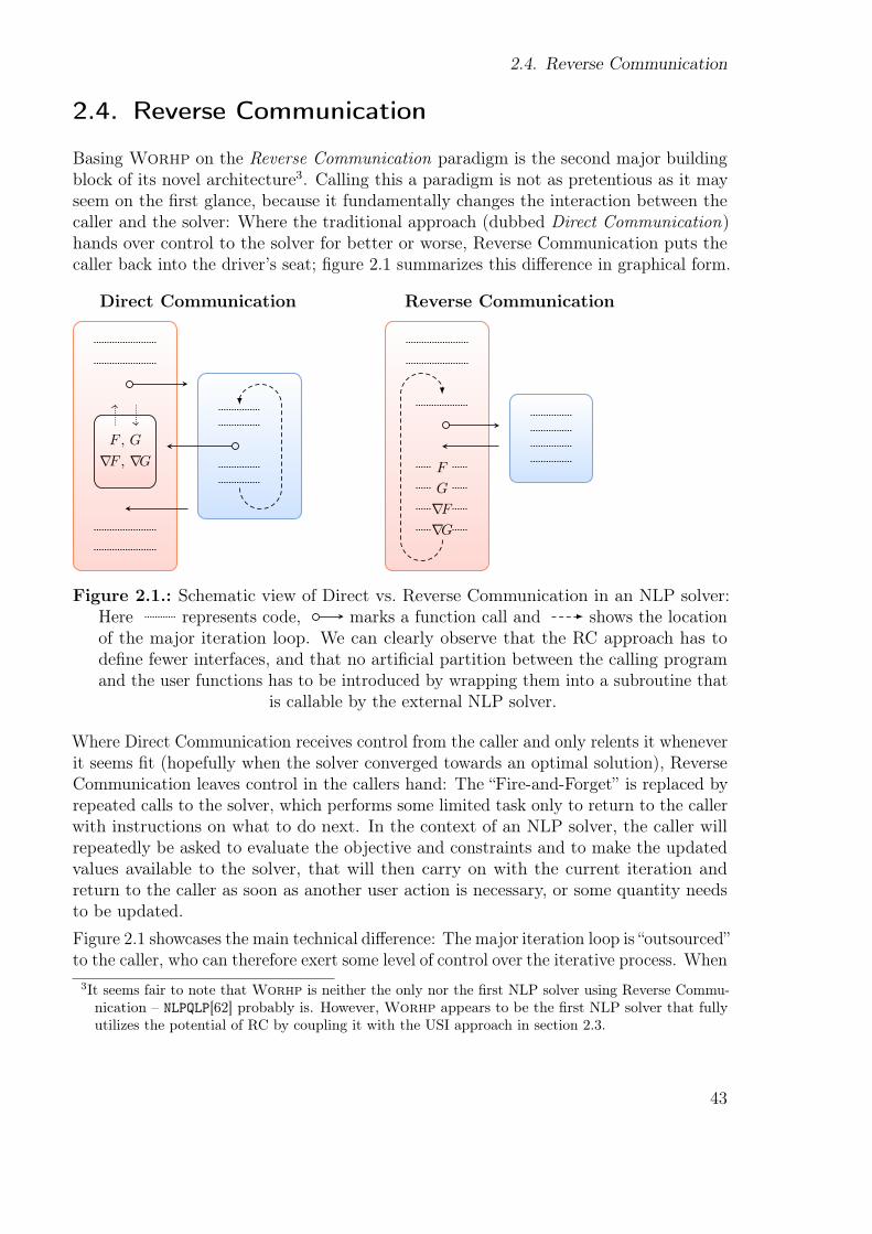
2.4. Reverse Communication
2.4. Reverse Communication
Basing Worhp on the Reverse Communication paradigm is the second major buildingblock of its novel architecture3. Calling this a paradigm is not as pretentious as it mayseem on the őrst glance, because it fundamentally changes the interaction between thecaller and the solver: Where the traditional approach (dubbed Direct Communication)hands over control to the solver for better or worse, Reverse Communication puts thecaller back into the driver’s seat; őgure 2.1 summarizes this diference in graphical form.
Direct Communication
F , G
∇F , ∇G
Reverse Communication
F
G
∇F∇G
Figure 2.1.: Schematic view of Direct vs. Reverse Communication in an NLP solver:Here represents code, marks a function call and shows the locationof the major iteration loop. We can clearly observe that the RC approach has todeőne fewer interfaces, and that no artiőcial partition between the calling programand the user functions has to be introduced by wrapping them into a subroutine that
is callable by the external NLP solver.
Where Direct Communication receives control from the caller and only relents it wheneverit seems őt (hopefully when the solver converged towards an optimal solution), ReverseCommunication leaves control in the callers hand: The łFire-and-Forgetž is replaced byrepeated calls to the solver, which performs some limited task only to return to the callerwith instructions on what to do next. In the context of an NLP solver, the caller willrepeatedly be asked to evaluate the objective and constraints and to make the updatedvalues available to the solver, that will then carry on with the current iteration andreturn to the caller as soon as another user action is necessary, or some quantity needsto be updated.
Figure 2.1 showcases the main technical diference: The major iteration loop is łoutsourcedžto the caller, who can therefore exert some level of control over the iterative process. When
3It seems fair to note that Worhp is neither the only nor the first NLP solver using Reverse Commu-nication – NLPQLP[62] probably is. However, Worhp appears to be the first NLP solver that fullyutilizes the potential of RC by coupling it with the USI approach in section 2.3.
43
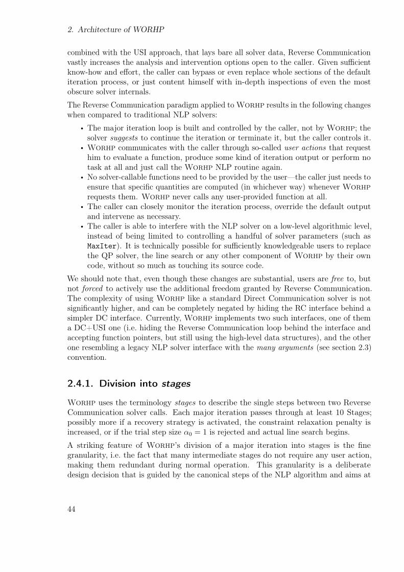
2. Architecture of WORHP
combined with the USI approach, that lays bare all solver data, Reverse Communicationvastly increases the analysis and intervention options open to the caller. Given suicientknow-how and efort, the caller can bypass or even replace whole sections of the defaultiteration process, or just content himself with in-depth inspections of even the mostobscure solver internals.
The Reverse Communication paradigm applied to Worhp results in the following changeswhen compared to traditional NLP solvers:
• The major iteration loop is built and controlled by the caller, not by Worhp; thesolver suggests to continue the iteration or terminate it, but the caller controls it.
• Worhp communicates with the caller through so-called user actions that requesthim to evaluate a function, produce some kind of iteration output or perform notask at all and just call the Worhp NLP routine again.
• No solver-callable functions need to be provided by the userÐthe caller just needs toensure that speciőc quantities are computed (in whichever way) whenever Worhp
requests them. Worhp never calls any user-provided function at all.• The caller can closely monitor the iteration process, override the default output
and intervene as necessary.• The caller is able to interfere with the NLP solver on a low-level algorithmic level,
instead of being limited to controlling a handful of solver parameters (such asMaxIter). It is technically possible for suiciently knowledgeable users to replacethe QP solver, the line search or any other component of Worhp by their owncode, without so much as touching its source code.
We should note that, even though these changes are substantial, users are free to, butnot forced to actively use the additional freedom granted by Reverse Communication.The complexity of using Worhp like a standard Direct Communication solver is notsigniőcantly higher, and can be completely negated by hiding the RC interface behind asimpler DC interface. Currently, Worhp implements two such interfaces, one of thema DC+USI one (i.e. hiding the Reverse Communication loop behind the interface andaccepting function pointers, but still using the high-level data structures), and the otherone resembling a legacy NLP solver interface with the many arguments (see section 2.3)convention.
2.4.1. Division into stages
Worhp uses the terminology stages to describe the single steps between two ReverseCommunication solver calls. Each major iteration passes through at least 10 Stages;possibly more if a recovery strategy is activated, the constraint relaxation penalty isincreased, or if the trial step size α0 = 1 is rejected and actual line search begins.
A striking feature of Worhp’s division of a major iteration into stages is the őnegranularity, i.e. the fact that many intermediate stages do not require any user action,making them redundant during normal operation. This granularity is a deliberatedesign decision that is guided by the canonical steps of the NLP algorithm and aims at
44
2.4. Reverse Communication
Worhp Caller
Pre
KKT
DF
DG
Check
KKT
HMiterationoutput
Create
QP
Update
Hessian
Solve
QP
Post
QP
Find
step sizeUpdate
Point
F G
Finalize
Figure 2.2.: Graphic representation of Worhp’s major stages. The stages are traversedin counter-clockwise order, with optional loops or jumps between them. Every stagereturns back to the caller, who then calls Worhp again to activate the next stage.The green 3rd-level nodes denote actions (mostly evaluations) that are required of the
caller before transitioning to the next stage.
exposing these steps to potential caller intervention. This design decision also accountsfor simplifying the solver-internal control ŕow, since many stages may jump to other(hitherto unmentioned) non-default stages to recover from errors or switch the solver into
45
2. Architecture of WORHP
diferent operational modes. The current design with frequent entry and return allows fora clean implementation of this complex control ŕow without having to resort to mutuallyentwined sequences of goto and jump marks at arbitrary code points.
2.4.2. Implementation considerations
Since most users will be content with the default behavior of the solver, the more extremescenarios of interventions are limited to few occasions, and the overhead of Reverse overDirect Communication is of interest to a majority of the users. The implementation thushas to strive to keep this overhead low.
Since the caller repeatedly polls for user actions and solver status, the implementationneeds to provide simple and eicient means to this end. There exist software packagescommunicating through RC that approach the ŕow control and user action issue througha single status integer whose value encodes the solver status, user actions and the currentor next stage of the solver. While this approach is indeed simple, its Achilles heel is thecoupling of unrelated entities. Worhp can currently request the user actions
1. Call worhp()
This user action is needed because the RC őnite diference routine temporarilyłswitches ofž Worhp and takes control of the RC loop itself to request functionevaluations.
2. Produce iteration output
The combination of USI and RC enables users to provide their own output routines,for instance because they prefer the clunky output of SNOPT, or because theoutput is further processed by text parsers that expect a speciőc format. Since thisaction is ŕagged exactly once per major iteration, it can also serve for user-speciőclogging, to ŕag a repaint of a graphical representation of the progress, or any otheraction that is performed once per major iteration.
3. Evaluate F
4. Evaluate G
5. Evaluate DF
6. Evaluate DG
7. Evaluate HM
The above ŕags prompt the caller to evaluate one of the user-deőned functions, orto update a derivative of them. It is important that the derivative ŕags are notraised, if the user chooses to have them approximated by őnite diferences or oneof the BFGS methods.
8. call finite difference routine to compute DF
9. call finite difference routine to compute DG
46
2.4. Reverse Communication
10. call finite difference routine to compute HM
11. call finite difference routine (catch-all of the above)
The őnite diference routine must also communicate through RC, and thus has aset of user actions. The őrst three actually confound solver status and user action,but the catch-all is used to hide this from the user.
In addition to these 11 user actions, Worhp has 49 distinct statuses [sic] and 16 stageswhich allows a total of 276 combinations (although most of no practical relevance), whichoverŕows the range of common integer types. Even if the number of combinations weremuch lower, it is a maintenance, book-keeping and documentation burden to keep trackof an extensive list of integers and their respective meanings. The obvious solution is tosplit status, stage and user action, and to introduce means to set, poll and reset them.
An NLP solver status (łiteratingž, łerrorž, łoptimal solution foundž etc.) can aptly berepresented by a simple integer number, since it cannot attain two distinct statuses atany time. This remains true for Worhp, but it can attain a superposition of statuses,if it terminates inside łacceptablež tolerances due to some error or limit conditionÐthe acceptable status is then superposed with the original stopping condition. Namedconstants are deőned by Worhp to avoid the use of magic numbers in user and librarycode to set or check for the status of the solver, for instance for the stopping criterion ofthe RC loop (Fortran version):
DO WHILE (cnt%status < terminateSuccess .AND. cnt%status > terminateError)
which is śeven without any comment or external documentationś signiőcantly more de-scriptive through the use of terminateSuccess and terminateError than the equivalentcondition
DO WHILE (cnt%status < 1000 .AND. cnt%status > -1000)
by inserting the numeric values of the constants. Furthermore, the version using namedconstants continues to function (after recompiling), even if the actual numeric valueschange, while the magic number version will break.
Worhp stages can be represented by an integer, as well, but it may be beneőcial forthe solver to be able to look back at previous stages, if the current behavior depends onwhich stages were traversed before, and also to plan ahead for more than one single stage.The appropriate structure to provide this functionality is a ring bufer, whose maximumlength is determined by the desired planning and retrospection horizons. Since a ringbufer is (slightly) more complex to handle than integer ŕags, getter and setter routinesare needed; Worhp provides GetStage and SetStage routines that query or schedulestages and abstract from the ring bufer implementation. For the actual representationof the stages, Worhp deőnes named constants of the form Init_SQP, Check_KKT etc.By convention, stage constants are formed with underscores, while status constants suchas OptimalSolution or TerminatedByUser are composed according to the CamelCaseconvention.
47
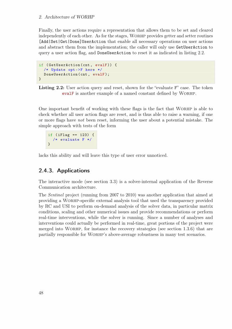
2. Architecture of WORHP
Finally, the user actions require a representation that allows them to be set and clearedindependently of each other. As for the stages, Worhp provides getter and setter routines[Add|Set|Get|Done]UserAction that enable all necessary operations on user actionsand abstract them from the implementation; the caller will only use GetUserAction toquery a user action ŕag, and DoneUserAction to reset it as indicated in listing 2.2.
if (GetUserAction(cnt , evalF)) {
/* Update opt ->F here */
DoneUserAction(cnt , evalF);
}
Listing 2.2: User action query and reset, shown for the łevaluate Fž case. The tokenevalF is another example of a named constant deőned by Worhp.
One important beneőt of working with these ŕags is the fact that Worhp is able tocheck whether all user action ŕags are reset, and is thus able to raise a warning, if oneor more ŕags have not been reset, informing the user about a potential mistake. Thesimple approach with tests of the form
if (iFlag == 123) {
/* evaluate F */
}
lacks this ability and will leave this type of user error unnoticed.
2.4.3. Applications
The interactive mode (see section 3.3) is a solver-internal application of the ReverseCommunication architecture.
The Sentinel project (running from 2007 to 2010) was another application that aimed atproviding a Worhp-speciőc external analysis tool that used the transparency providedby RC and USI to perform on-demand analysis of the solver data, in particular matrixconditions, scaling and other numerical issues and provide recommendations or performreal-time interventions, while the solver is running. Since a number of analyses andinterventions could actually be performed in real-time, great portions of the project weremerged into Worhp, for instance the recovery strategies (see section 1.3.6) that arepartially responsible for Worhp’s above-average robustness in many test scenarios.
48
2.5. Serialization
2.5. Serialization
The serialization module is a natural extension of Worhp’s data handling: It enablesserialization of the data structures to a őle, and vice versa, deserialization from a őleback to the data structures, i.e. it deőnes a one-to-one mapping between the in-memoryrepresentation of the C structs used by Worhp and a őle on disk.
Since Worhp is stateless by design, this allows to completely capture the solver state.
2.5.1. Hotstart functionality
The most prominent application of the serialization module is the Hotstart functionality ofWorhp, which allows to save and restore an optimization process. To this end, the solveris interrupted between any two stages (see section 2.4.1) and terminated after serializingits state. The state őle can later be loaded by Worhp, producing bit-precise restorationsof its state, which enables seamless continuation of the previously interrupted iteration.This seamless continuation is the deőning capability of the Hotstart functionality and setsit apart from the warm start feature of other NLP solvers, which mostly includes restoringthe BFGS matrix and possibly the multipliers, but disregards the signiőcant internal state,such as penalty parameters (when using a merit function), the őlter entries (when insteadusing a őlter), best-so-far solution etc. If the Hotstart őle is platform-independent (whichit is, as outlined in section 2.5.3), users can migrate an optimization run between diferentcomputers and architectures, for instance from Linux to Windows, from 32-bit systemsto 64-bit ones, from PowerPC to Itanium. Hotstart őles are written by WorhpToXML
and HotstartSave (Fortran/C), and read by WorhpFromXML and HotstartLoad. Theroutine names difer, because the C functions are wrappers around the Fortran routinesthat make heavy use of optional arguments, which is not readily portable to C using theestablished Fortran standard.
2.5.2. Reading parameters
In addition to the complete Hotstart, it is possible to perform an incomplete Hotstart byusing only partial information; this may consist of a single data structure only or of agenuine subset of components, leaving the missing ones at default values. The obvious(and historically the őrst) application of this option is to outőt Worhp with a parameterőle from which to read its parameters at runtime. This parameter őle is technically anincomplete Hotstart őle, which contains an image of the Params data structure only. Theőle may even be incomplete, in the sense of omitting some components, if one wishesto set only few, instead of all parameters, to speciőc values. This is enabled by őrstusing the default initializer, followed by checking the presence of every component inthe parameter őle, overriding the initialized default value. Fortran callers can use theWorhpFromXML routine for reading incomplete Hotstart őles (using optional arguments,as laid out earlier), while C callers are provided with the tailored ReadXML function.
49
2. Architecture of WORHP
One user-driven extension to the parameter reading is the ability to provide defaultparameters that difer from Worhp’s defaults, while still allowing a parameter őle tooverride them. Since the usual initialize-override approach is atomic from the caller’sperspective, it cannot provide this functionality, because the initialization step overridesany caller-speciőc defaults. The solution is to separate both steps into two operations.Worhp provides a new InitParams routine to perform the initialization step, andnon-initializing parameter reading routine for the second; the Fortran WorhpFromXML isextended by an optional noInit ŕag, while C callers use the new ReadParamsNoInit
function.
2.5.3. Serialization format
The choice of a serialization format was guided by the following constraints:
Readability: Hotstart and, more importantly, parameter őles should be easily human-readable, and editing them should be possible without imposing rigid formattingrules on users. This precludes the use of binary formats, even though they are moreeicient.
Portability: Both Hotstart and parameter őles must not be platform-dependent; porta-bility of the Hotstart őle between platforms is an explicit feature. The same isvalid for parameter őles, since the solver is supposed to show consistent results4
when running the same problem with the same parameter on diferent platforms.This, again, discourages the use of binary formats.
Standardization: If possible, the serialization format should conform to an establishedstandard. This way, external tools will be available to edit or perform moresophisticated operations on the serialization őles. Availability of syntax highlightingin an editor is tangible example for this demand.
Efficiency: With Worhp being designed for large-scale optimization, Hotstart őlespotentially need to hold a considerable amount of data. The serialization formatshould cause as little overhead as possible, although this goal contradicts readabilityand portability, since it essentially calls for a binary format.
Possible candidates are JSON, YAML and XML. Despite their diferences, for instancein supporting types other than strings, none is signiőcantly superior to the others for ourpurposes. Two arguments initially supported the choice of XML as Worhp’s serializationformat:
• XML is rather robust, whereas whitespace changes can signiőcantly change theinterpretation of (read: break) YAML data.
4Demanding equal behavior between platforms is unrealistic, since different processors, compilers andmath libraries have subtle influences on the results of floating point arithmetic; instead we canrealistically only demand consistent results and differences in the order of 1 ulp, unless such errorsaccumulate.
50

2.5. Serialization
• Most, if not all, unixoid operating systems come equipped with libxml2, whichseemed to facilitate portability in the initial development.
While the robustness argument is still valid, subtle diferences between Linux distributions(most noticeable symbol versioning), make short work of portability. The internal XMLparser presented in section 3.5 has therefore been added in late 2012 to cut dependencieson external tools. This in turn invalidates the second argument and opens the roadto considering an alternative serialization format, since the XML grammar (and theresulting parser) is quite intricate and complex.
51


Chapter3
Technical Implementation
The compiler does not change its operation to conform to themeanings implied by your variable names.
(Quip on GCC Bugzilla)
3.1. Hybrid implementation . . . . . . . . . . . . . . . . . . . . . . . . 55
3.1.1. Interoperability issues . . . . . . . . . . . . . . . . . . . . 55
3.1.2. Interoperability improvements . . . . . . . . . . . . . . . . 59
3.1.3. Data structure handling in Worhp . . . . . . . . . . . . . 63
3.2. Automatic code generation . . . . . . . . . . . . . . . . . . . . . 68
3.2.1. Data structure definition . . . . . . . . . . . . . . . . . . . 69
3.2.2. Definition file . . . . . . . . . . . . . . . . . . . . . . . . . 70
3.2.3. Template files . . . . . . . . . . . . . . . . . . . . . . . . 72
3.2.4. Applications of automatic code generation . . . . . . . . . 73
3.3. Interactive mode . . . . . . . . . . . . . . . . . . . . . . . . . . . 76
3.4. Workspace Management . . . . . . . . . . . . . . . . . . . . . . . 79
3.4.1. Automatic workspace management . . . . . . . . . . . . . 79
3.4.2. Dedicated dynamic memory . . . . . . . . . . . . . . . . . 81
3.5. Internal XML parser . . . . . . . . . . . . . . . . . . . . . . . . . 85
3.6. Established shortcomings, bugs and workarounds . . . . . . . . . . 87
3.6.1. Intel Visual Fortran 10.1 . . . . . . . . . . . . . . . . . . . 87
3.6.2. Windows . . . . . . . . . . . . . . . . . . . . . . . . . . . 87
3.7. Maintaining compatibility across versions . . . . . . . . . . . . . . 89
53

3. Technical Implementation
This chapter is concerned with the (software-)engineering details needed to implementthe architecture and functionality outlined in the previous chapters.
The main aspects under consideration are:
• the mixed-language (hybrid) implementation of Worhp, which aims at harvestingthe beneőts of both C and Fortran and facilitates interfacing with both languagesin a łnaturalž way;
• the automatic code generation, which became a technical necessity as the size andtechnical complexity of Worhp increased and has since then been established andextended to a convenient tool for relieving developers of many onerous tasks;
• the workspace management used by Worhp to handle dynamic memory require-ments;
• the technical infrastructure to build the various solver interfaces for a wide rangeof conőgurations and target platforms, in a mostly automatic way, and to performother maintenance or technical tasks.
54
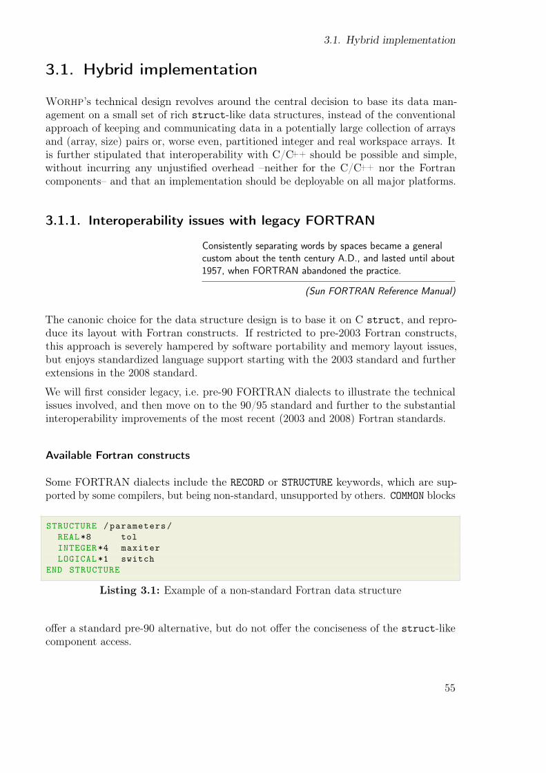
3.1. Hybrid implementation
3.1. Hybrid implementation
Worhp’s technical design revolves around the central decision to base its data man-agement on a small set of rich struct-like data structures, instead of the conventionalapproach of keeping and communicating data in a potentially large collection of arraysand (array, size) pairs or, worse even, partitioned integer and real workspace arrays. Itis further stipulated that interoperability with C/C++ should be possible and simple,without incurring any unjustiőed overhead śneither for the C/C++ nor the Fortrancomponentsś and that an implementation should be deployable on all major platforms.
3.1.1. Interoperability issues with legacy FORTRAN
Consistently separating words by spaces became a generalcustom about the tenth century A.D., and lasted until about1957, when FORTRAN abandoned the practice.
(Sun FORTRAN Reference Manual)
The canonic choice for the data structure design is to base it on C struct, and repro-duce its layout with Fortran constructs. If restricted to pre-2003 Fortran constructs,this approach is severely hampered by software portability and memory layout issues,but enjoys standardized language support starting with the 2003 standard and furtherextensions in the 2008 standard.
We will őrst consider legacy, i.e. pre-90 FORTRAN dialects to illustrate the technicalissues involved, and then move on to the 90/95 standard and further to the substantialinteroperability improvements of the most recent (2003 and 2008) Fortran standards.
Available Fortran constructs
Some FORTRAN dialects include the RECORD or STRUCTURE keywords, which are sup-ported by some compilers, but being non-standard, unsupported by others. COMMON blocks
STRUCTURE /parameters/
REAL*8 tol
INTEGER *4 maxiter
LOGICAL *1 switch
END STRUCTURE
Listing 3.1: Example of a non-standard Fortran data structure
ofer a standard pre-90 alternative, but do not ofer the conciseness of the struct-likecomponent access.
55
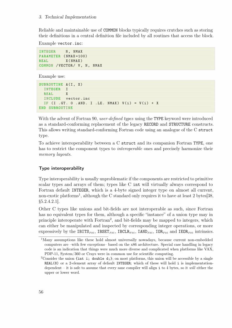
3. Technical Implementation
Reliable and maintainable use of COMMON blocks typically requires crutches such as storingtheir deőnitions in a central deőnition őle included by all routines that access the block.
Example vector.inc:
INTEGER N, NMAX
PARAMETER (NMAX =100)
REAL X(NMAX)
COMMON /VECTOR/ V, N, NMAX
Example use:
SUBROUTINE A(I, X)
INTEGER I
REAL X
INCLUDE vector.inc
IF (I .GT. 0 .AND. I .LE. NMAX) V(i) = V(i) + X
END SUBROUTINE
With the advent of Fortran 90, user-defined types using the TYPE keyword were introducedas a standard-conforming replacement of the legacy RECORD and STRUCTURE constructs.This allows writing standard-conforming Fortran code using an analogue of the C struct
type.
To achieve interoperability between a C struct and its companion Fortran TYPE, onehas to restrict the component types to interoperable ones and precisely harmonize theirmemory layouts.
Type interoperability
Type interoperability is usually unproblematic if the components are restricted to primitivescalar types and arrays of them; types like C int will virtually always correspond toFortran default INTEGER, which is a 4-byte signed integer type on almost all current,non-exotic platforms1, although the C standard only requires it to have at least 2 bytes[38,ğ5.2.4.2.1].
Other C types like unions and bit-őelds are not interoperable as such, since Fortranhas no equivalent types for them, although a speciőc łinstancež of a union type may inprinciple interoperate with Fortran2, and bit-őelds may be mapped to integers, whichcan either be manipulated and inspected by corresponding integer operations, or moreexpressively by the IBITSF95 , IBSETF95 , IBCLRF95 , IANDF95 , IORF95 and IEORF95 intrinsics.
1Many assumptions like these hold almost universally nowadays, because current non-embeddedcomputers are –with few exceptions– based on the x86 architecture. Special case handling in legacycode is an indication that things were much more diverse and complicated when platforms like VAX,PDP-11, System/360 or Crays were in common use for scientific computing.
2Consider the union {int i; double d;}; on most platforms, this union will be accessible by a singleREAL(8) or a 2-element array of default INTEGER; which of these will hold i is implementation-dependent – it is safe to assume that every sane compiler will align i to 4 bytes, so it will either theupper or lower word.
56
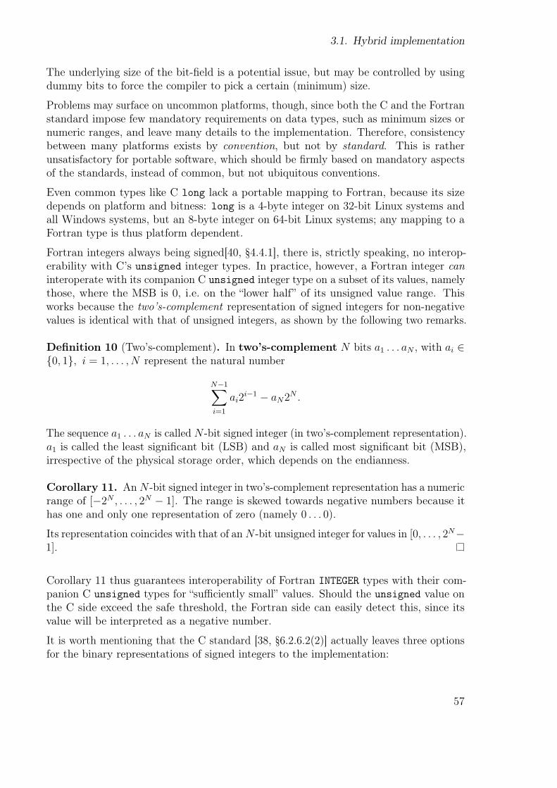
3.1. Hybrid implementation
The underlying size of the bit-őeld is a potential issue, but may be controlled by usingdummy bits to force the compiler to pick a certain (minimum) size.
Problems may surface on uncommon platforms, though, since both the C and the Fortranstandard impose few mandatory requirements on data types, such as minimum sizes ornumeric ranges, and leave many details to the implementation. Therefore, consistencybetween many platforms exists by convention, but not by standard. This is ratherunsatisfactory for portable software, which should be őrmly based on mandatory aspectsof the standards, instead of common, but not ubiquitous conventions.
Even common types like C long lack a portable mapping to Fortran, because its sizedepends on platform and bitness: long is a 4-byte integer on 32-bit Linux systems andall Windows systems, but an 8-byte integer on 64-bit Linux systems; any mapping to aFortran type is thus platform dependent.
Fortran integers always being signed[40, ğ4.4.1], there is, strictly speaking, no interop-erability with C’s unsigned integer types. In practice, however, a Fortran integer caninteroperate with its companion C unsigned integer type on a subset of its values, namelythose, where the MSB is 0, i.e. on the łlower halfž of its unsigned value range. Thisworks because the two’s-complement representation of signed integers for non-negativevalues is identical with that of unsigned integers, as shown by the following two remarks.
Definition 10 (Two’s-complement). In two’s-complement N bits a1 . . . aN , with ai ∈{0, 1}, i = 1, . . . , N represent the natural number
N−1
i=1
ai2i−1 − aN2
N .
The sequence a1 . . . aN is called N -bit signed integer (in two’s-complement representation).a1 is called the least signiőcant bit (LSB) and aN is called most signiőcant bit (MSB),irrespective of the physical storage order, which depends on the endianness.
Corollary 11. An N -bit signed integer in two’s-complement representation has a numericrange of [−2N , . . . , 2N − 1]. The range is skewed towards negative numbers because ithas one and only one representation of zero (namely 0 . . . 0).
Its representation coincides with that of an N -bit unsigned integer for values in [0, . . . , 2N−1].
Corollary 11 thus guarantees interoperability of Fortran INTEGER types with their com-panion C unsigned types for łsuiciently smallž values. Should the unsigned value onthe C side exceed the safe threshold, the Fortran side can easily detect this, since itsvalue will be interpreted as a negative number.
It is worth mentioning that the C standard [38, ğ6.2.6.2(2)] actually leaves three optionsfor the binary representations of signed integers to the implementation:
57

3. Technical Implementation
a) sign-and-magnitude: bits a1 . . . aN−1 are value bits and the sign bit aN is a genuinesign bit, analogous to the IEEE ŕoating point data types.
b) one’s-complement: the sign bit has value −(2N − 1).
c) two’s-complement: the sign bit has value −2N as described in Deőnition 10.
Since options a) and b) have computationally relevant issues (two representations of zeroand non-trivial addition), modern platforms exclusively use c) for integer representation.
Memory layout
Matching the structures’ memory layout is, by far, the more problematic issue withinteroperability. A structure maps its components into memory by deőning for eachcomponent an ofset from the beginning of a structure instance, as illustrated by őgure 3.1.Therefore, the memory layout between a C struct and its companion Fortran TYPE
matches, if both structures have components of pairwise equal storage sizes and sharethe same ofset mapping.
base
8byte
int i size = 4
offset = 0
internal
padding
double x size = 8
offset = 8
int j size = 4
offset = 16
tail
paddingstruct size = 24
sizes = 16
struct {
int i;
double x;
int j;
}
memory layout
Figure 3.1.: Schematic of data structure memory layout, assuming mandatory 8 bytealignment. Members are accessed in memory by ⟨base address⟩ + ⟨ofset⟩. Thealignment requirement (or rather the blunder in the ordering of the components)causes 25% overhead for padding due to the strict speciőcations of the C standard.
The C standard requires that these ofsets are increasing in the order of the components,but the Fortran standard does not prohibit reordering of the structure components; thiscan be inhibited by using the SEQUENCE attribute to the TYPE deőnition[40, ğ4.5.1.2].COMMON blocks may not be reordered[40, ğ5.5.2.1(1+2)] by the Fortran compiler3, whichis why it is customary among experienced Fortran developers to sort its components bysize to minimize the amount of padding added by the compiler: Both C[38, ğ6.7.2.1(12-13)] and Fortran[40, Note 4.20] compilers may add unnamed padding between adjacent
3This “allows” tricks such as accessing IA(1) in COMMON/IA(2),IB(2)/ through IB(-1).
58
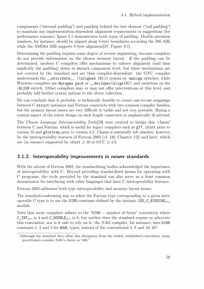
3.1. Hybrid implementation
components (łinternal paddingž) and padding behind the last element (łtail paddingž)to maintain any implementation-dependent alignment requirements or suggestions (forperformance reasons); őgure 3.1 demonstrates both types of padding. Double precisionnumbers, for instance, should be aligned along 4-byte boundaries according the 386 ABI,while the AMD64 ABI suggests 8 byte alignment[37, Figure 3-1].
Determining the padding requires some degree of reverse engineering, because compilersdo not provide information on the chosen memory layout. If the padding can bedetermined, modern C compilers ofer mechanisms to enforce alignment (and thusimplicitly the padding) down to struct component level, but these mechanisms arenot covered by the standard and are thus compiler-dependent: the GNU compilerunderstands the __attribute__ ((aligned (N))) syntax or -malign switches, whileWindows compilers use #pragma pack or __declspec(align(N)) and variations on the/ALIGN switch. Other compilers may or may not ofer interventions at this level, andprobably add further syntax options to the above collection.
We can conclude that it probably is technically feasible to create one-to-one mappingsbetween C struct instances and Fortran constructs with two common compiler families,but the memory layout issues are very diicult to tackle and not very portable. Basing acentral aspect of the solver design on such fragile constructs is emphatically ill-advised.
The Chasm Language Interoperability Tools[59] were created to bridge this łchasmžbetween C and Fortran, which is useful for legacy compilers such as g77, ifort prior toversion 10 and gfortran prior to version 4.3. Chasm is essentially left obsolete, however,by the interoperability features of Fortran 2003 (cf. [40, Chapter 15]) and later, whichare (in essence) supported by ifort > 10 or GCC > 4.3.
3.1.2. Interoperability improvements in newer standards
With the advent of Fortran 2003, the standardizing bodies acknowledged the importanceof interoperability with C. Beyond providing standardized means for operating withC programs, the tools provided by the standard can also serve as a least commondenominator for interfacing with other languages that have C interoperability features.
Fortran 2003 addresses both type interoperability and memory layout issues:
The standard-conforming way to select the Fortran type corresponding to a given inter-operable C type is to use the KIND constants deőned by the intrinsic ISO_C_BINDINGF03
module.
Note that most compilers adhere to the łKIND = number of bytesž convention whereC_INTF03 is 4 and C_DOUBLEF03 is 8, but neither does the standard require or advocatethis convention, nor is it safe to rely on it: the NAG compiler, for instance, uses KINDconstants 1, 2 and 3 for REAL types, instead of the conventional 4, 8 and 10/164.
4Although the standard does allow this divergence from the widely established convention, manypractitioners consider NAG’s choice as “silly”.
59

3. Technical Implementation
C type Fortran 2003 type Noteint INTEGER(KIND=C_INT) 4 with most compilerslong INTEGER(KIND=C_LONG) 4 or 8 with most compilerssize_t INTEGER(KIND=C_SIZE_T) size_t is unsigned!float REAL(KIND=C_FLOAT) 4 with most compilersdouble REAL(KIND=C_DOUBLE) 8 with most compilerschar CHARACTER(KIND=C_CHAR) see note on string interoperability_BoolC99 LOGICAL(KIND=C_BOOL)
Table 3.1.: Interoperable scalar types deőned by ISO_C_BINDINGF03 (incomplete list).
The standard-conforming way to match the memory layout of a user-deőned TYPE isto add the BIND(C) modiőer to its deőnition, as shown in listing 3.2. In words of thestandard:
A Fortran derived type is interoperable with a C struct type if the derived-type definition of the Fortran type specifies BIND(C), the Fortran derivedtype and the C struct type have the same number of components, and thecomponents of the Fortran derived type have types and type parameters thatare interoperable with the types of the corresponding components of the structtype. A component of a Fortran derived type and a component of a C structtype correspond if they are declared in the same relative position in theirrespective type definitions. [40, ğ15.2.3]
By adding the BIND(C) modiőer we instruct the Fortran compiler to
• check all structure components for their interoperability,• not reorder the structure components, as if SEQUENCE were in efect,• use the same padding as the companion C compiler for the equivalent C struct.
Using the ISO_C_BINDINGF03 features, we can thus create Fortran user-deőned TYPEs thathave a matching C struct, although both languages have non-interoperable constructsfor which there is no equivalent construct in the respective other language. Examplesinclude union and bit-őelds in C, and ALLOCATABLE or POINTER types in Fortran.
TYPE , BIND(C) :: MyInteroperableType
REAL(KIND=C_DOUBLE) :: X(3)
INTEGER(KIND=C_INT) :: N
END TYPE MyInteroperableType
Listing 3.2: Example of a C-interoperable Fortran type
Interoperability of strings is not as straightforward as the one-to-one mapping betweenthe numeric types, since they are łőrst-class citizensž in Fortran. The LEN attributegives them a őxed length, such that no 0-termination is necessary, whereas in C, stringsare (pointers to) character arrays, and their (string-)length is deőned by the position of
60

3.1. Hybrid implementation
struct MyInteroperableStruct {
double X[3];
int n;
}
Listing 3.3: C struct corresponding to the Fortran type in listing 3.2.
the 0-character. As component of a user-deőned type, a CHAR(KIND=C_CHAR, LEN=N) ::
string may be mapped to a char string[N+1] when care is taken of 0-termination andthe undeőned characters between the logical and the physical string length are initializedto blanks:
• If 0-termination is not maintained by the Fortran side, C routines accessing thestring may read past its end, resulting in trailing garbage characters in the outputand possible program termination by the OS due to illegal memory access.
• If the undeőned intermediate characters are not set to blanks by the C side, Fortranroutines accessing the string will use them until all LEN=N characters have beenprocessed, resulting in garbage characters in the output.
Fortran can add 0-termination by setting string(L+1:L+1) = C_NULL_CHARF03 (whereL 6 N is the number of characters; notice the slice-like syntax needed for accessing asingle character, since Fortran strings are syntactically different from arrays of characters,although their in-memory representation is identical).
Since Fortran types with ALLOCATABLE or POINTER attribute are not (yet5) interoperable,dynamic arrays have to be implemented on the C side. Fortran can interoperate withC pointers through the TYPE(C_PTR)F03 type, deőned by the ISO_C_BINDINGF03 module.Allocated C pointers cannot be directly accessed by Fortran, since Fortran arrays andpointers in addition to their type also have extent information, which C pointers arelacking. To create a Fortran pointer from an allocated C pointer, the C_F_POINTERF03
routine takes a TYPE(C_PTR)F03 , extent information and initializes a Fortran pointer(note that TYPE(C_PTR)F03 is type-agnostic, hence the Fortran pointer type has to matchthe C pointer type, or accessing it may result in undeőned behavior).
Interoperable functions
With types being interoperable, the next step is to consider interoperability of functions.While Fortran diferentiates between functions and subroutines, from a C point of viewthe latter is the same as the őrst with no return value, i.e. void, hence we only need toconsider functions (in C sense) without worrying about special treatment for (Fortran)subroutines.
5TR 29113 of JTC1/SC22/WG5 introduced ISO_Fortran_binding.h as header file provided by thecompanion C compiler to define an opaque Fortran array-descriptor type and macros to access theFortran array and dimensions. Unfortunately, this part of the technical report was not adopted bythe standardazing body and thus remains in limbo.
61

3. Technical Implementation
For a function to be interoperable, all of its arguments have to be interoperable andthe types and order of function arguments have to match. Again, the BIND(C) modiőerinstructs the compiler to check for interoperability and behave cooperatively towards itscompanion C compiler. An important additional feature for functions is the ability tospecify their assembly name ś this is important, because Fortran compilers generallyperform name mangling, which not only difers between compiler vendors, but is alsoinŕuenced by the use (and naming) of encompassing modules; table 3.2 shows thesomewhat diverse name mangling conventions used by a selection of diferent compilers.Using the BIND(C, name="assembly_name") modiőer instructs the compiler to use thespeciőed name as assembly name, instead of the result of the compiler-speciőc namemangling scheme. This greatly simpliőes linking to C components in a portable way,since the assembly name can be chosen freely and works independently of the currentcompiler; it can even be used to make existing C functions (such as stdlib functions)available to Fortran ś a technique employed by Worhp’s workspace management anddescribed in detail in section 3.4.
SUBROUTINE foo_bar() becomes . . .
compiler freestanding inside module fred
g77/f2c foo_bar__ Ðgfortran (Linux) foo_bar_ __fred_MOD_foo_bar
gfortran (MinGW old winapi) _foo_bar_ ___fred_MOD_foo_bar
gfortran (MinGW new winapi) foo_bar_ __fred_MOD_foo_bar
ifort (Linux) foo_bar_ fred_mp_foo_bar_
ifort (Windows) _FOO_BAR _FRED_mp_FOO_BAR
Table 3.2.: Examples of Fortran name mangling with diferent compilers.
A minor complication is the fact that the so-called łargument associationž of Fortran isbest described as call-by-reference [40, ğ12.4.1], whereas C operates on local copies of allarguments, i.e. call-by-value [38, ğ6.5.2.2(4)]Ðthis explains why the following (invalid)FORTRAN program prints 2 when compiled with some legacy compilers:
PROGRAM INVALID
CALL PLUS (1)
PRINT *, 1
END PROGRAM
SUBROUTINE PLUS(I)
INTEGER I
I = I+1
END SUBROUTINE
(this will not work with modern compilers, since they perform more complete checkson arguments, and furthermore put the integer constant 1 into a read-only data section[ELF: .rodata], hence the program is killed by the OS with a memory access violationwhen PLUS tries to increment the value at this address.)
62
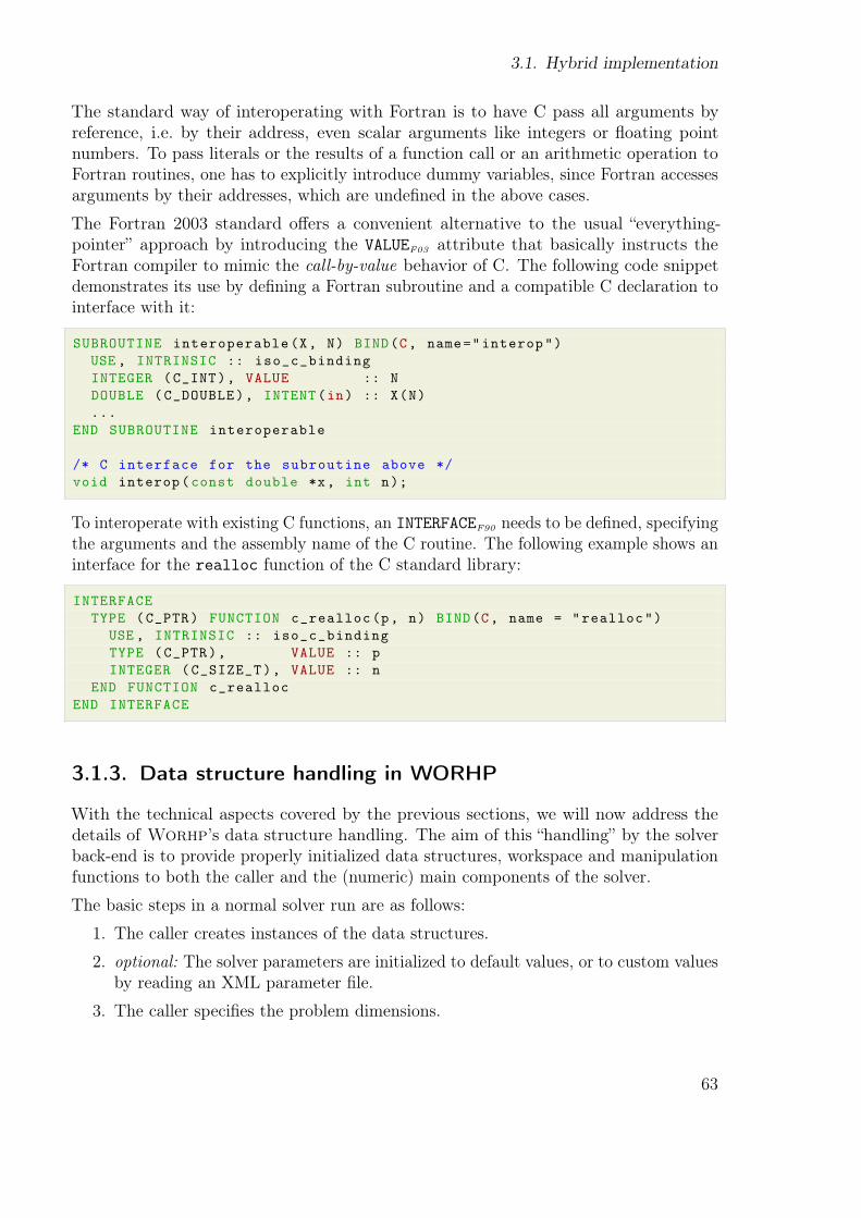
3.1. Hybrid implementation
The standard way of interoperating with Fortran is to have C pass all arguments byreference, i.e. by their address, even scalar arguments like integers or ŕoating pointnumbers. To pass literals or the results of a function call or an arithmetic operation toFortran routines, one has to explicitly introduce dummy variables, since Fortran accessesarguments by their addresses, which are undeőned in the above cases.
The Fortran 2003 standard ofers a convenient alternative to the usual łeverything-pointerž approach by introducing the VALUEF03 attribute that basically instructs theFortran compiler to mimic the call-by-value behavior of C. The following code snippetdemonstrates its use by deőning a Fortran subroutine and a compatible C declaration tointerface with it:
SUBROUTINE interoperable(X, N) BIND(C, name="interop")
USE , INTRINSIC :: iso_c_binding
INTEGER (C_INT), VALUE :: N
DOUBLE (C_DOUBLE), INTENT(in) :: X(N)
...
END SUBROUTINE interoperable
/* C interface for the subroutine above */
void interop(const double *x, int n);
To interoperate with existing C functions, an INTERFACEF90 needs to be deőned, specifyingthe arguments and the assembly name of the C routine. The following example shows aninterface for the realloc function of the C standard library:
INTERFACE
TYPE (C_PTR) FUNCTION c_realloc(p, n) BIND(C, name = "realloc")
USE , INTRINSIC :: iso_c_binding
TYPE (C_PTR), VALUE :: p
INTEGER (C_SIZE_T), VALUE :: n
END FUNCTION c_realloc
END INTERFACE
3.1.3. Data structure handling in WORHP
With the technical aspects covered by the previous sections, we will now address thedetails of Worhp’s data structure handling. The aim of this łhandlingž by the solverback-end is to provide properly initialized data structures, workspace and manipulationfunctions to both the caller and the (numeric) main components of the solver.
The basic steps in a normal solver run are as follows:
1. The caller creates instances of the data structures.
2. optional: The solver parameters are initialized to default values, or to custom valuesby reading an XML parameter őle.
3. The caller speciőes the problem dimensions.
63

3. Technical Implementation
4. The back-end initializes all data structures, allocating storage for variables, matrixstructures and workspace, and setting all counters, ŕags etc. to default values.
5. The caller speciőes initial values, bounds and the sparse matrix structures (ifavailable), using the previously allocated storage.
6. The caller starts the solver.
7. The solver, on its őrst call, uses the workspace handling routines to request anumber of workspace slices, depending on the dimensions and other input of thecaller, and continues its normal operation afterwards.
8. The solver requests additional workspace slices during its operation, either perma-nently (on-demand) or for temporary storage.
9. Upon reaching a termination criterion, the solver őnally returns to the caller, whowill usually save or otherwise process the results.
10. The back-end frees all allocated storage. The data structures can now be discardedor reused for another run, starting at 2.
1: Create instances
This will usually just consist of statically creating instances through
TYPE (OptVar) :: opt
TYPE (Workspace) :: wsp
TYPE (Params) :: par
TYPE (Control) :: cnt
OptVar opt;
Workspace wsp;
Params par;
Control cnt;
It is also possible in both languages to create pointers and allocate them at runtime. Atechnical complication of both approaches is the default initialization of the initializedŕag in every data structure that serves as a safeguard against overwriting of user-deőnedvalues by defaults and memory leaks through double allocation of pointers. Currentlythe caller has to ensure that the ŕag is false, or the back-end will skip all initialization.
A considerable extension of the approach to allocate pointers to the structures at run-timeis to employ the pimpl idiom discussed in section 3.7
2: Initialize parameters
The caller can optionally initialize the parameter structure, or leave it to the back-end to initialize it to default values. The usual approach is to use the XML module(cf. section 2.5) to read a complete or partial parameter őle to set all parameters tospeciőed values; parameters not present in the őle are set to their hard-coded defaults.
When Worhp is integrated into another piece of software, this behavior may be undesir-able, since the program may need to provide a diferent (sub)set of default parameters,while still allowing the parameter őle to override them. Section 2.5.2 describes howWorhp has decoupled initialization and parameter reading to accommodate these cases.
64
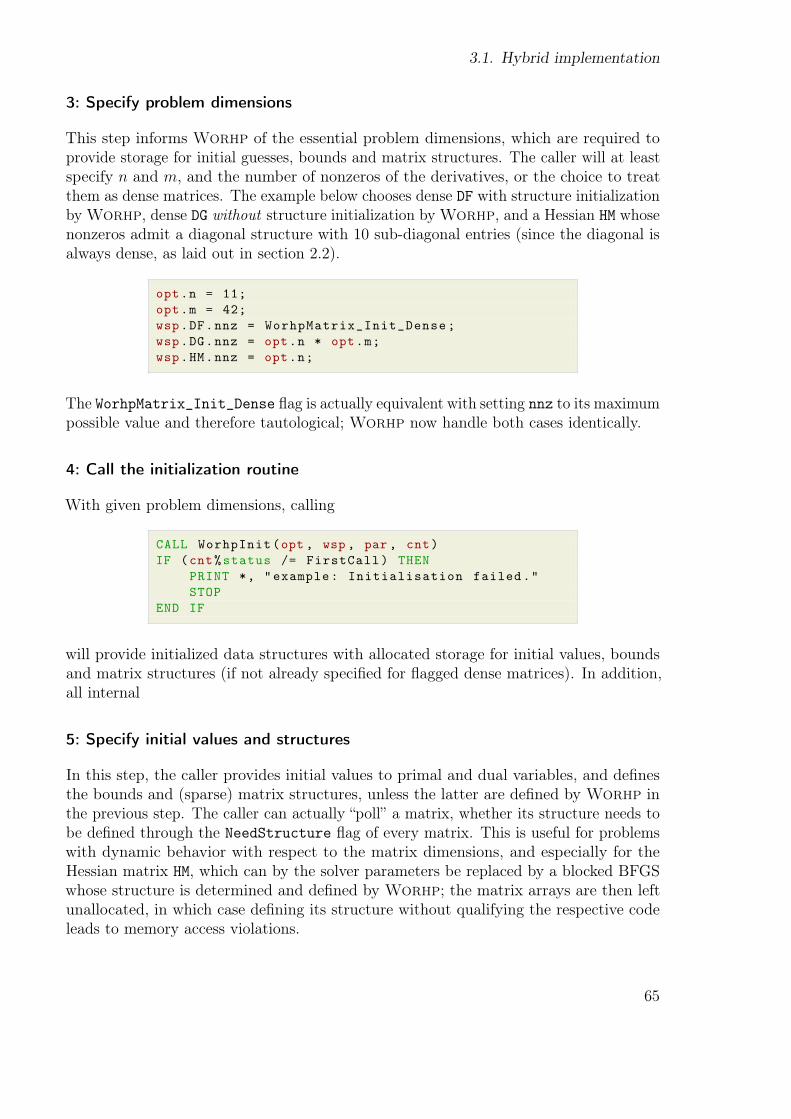
3.1. Hybrid implementation
3: Specify problem dimensions
This step informs Worhp of the essential problem dimensions, which are required toprovide storage for initial guesses, bounds and matrix structures. The caller will at leastspecify n and m, and the number of nonzeros of the derivatives, or the choice to treatthem as dense matrices. The example below chooses dense DF with structure initializationby Worhp, dense DG without structure initialization by Worhp, and a Hessian HM whosenonzeros admit a diagonal structure with 10 sub-diagonal entries (since the diagonal isalways dense, as laid out in section 2.2).
opt.n = 11;
opt.m = 42;
wsp.DF.nnz = WorhpMatrix_Init_Dense;
wsp.DG.nnz = opt.n * opt.m;
wsp.HM.nnz = opt.n;
The WorhpMatrix_Init_Dense ŕag is actually equivalent with setting nnz to its maximumpossible value and therefore tautological; Worhp now handle both cases identically.
4: Call the initialization routine
With given problem dimensions, calling
CALL WorhpInit(opt , wsp , par , cnt)
IF (cnt%status /= FirstCall) THEN
PRINT *, "example: Initialisation failed."
STOP
END IF
will provide initialized data structures with allocated storage for initial values, boundsand matrix structures (if not already speciőed for ŕagged dense matrices). In addition,all internal
5: Specify initial values and structures
In this step, the caller provides initial values to primal and dual variables, and deőnesthe bounds and (sparse) matrix structures, unless the latter are deőned by Worhp inthe previous step. The caller can actually łpollž a matrix, whether its structure needs tobe deőned through the NeedStructure ŕag of every matrix. This is useful for problemswith dynamic behavior with respect to the matrix dimensions, and especially for theHessian matrix HM, which can by the solver parameters be replaced by a blocked BFGSwhose structure is determined and deőned by Worhp; the matrix arrays are then leftunallocated, in which case deőning its structure without qualifying the respective codeleads to memory access violations.
65
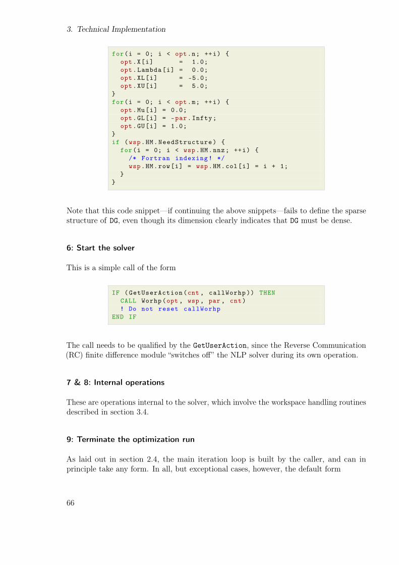
3. Technical Implementation
for(i = 0; i < opt.n; ++i) {
opt.X[i] = 1.0;
opt.Lambda[i] = 0.0;
opt.XL[i] = -5.0;
opt.XU[i] = 5.0;
}
for(i = 0; i < opt.m; ++i) {
opt.Mu[i] = 0.0;
opt.GL[i] = -par.Infty;
opt.GU[i] = 1.0;
}
if (wsp.HM.NeedStructure) {
for(i = 0; i < wsp.HM.nnz; ++i) {
/* Fortran indexing! */
wsp.HM.row[i] = wsp.HM.col[i] = i + 1;
}
}
Note that this code snippetÐif continuing the above snippetsÐfails to deőne the sparsestructure of DG, even though its dimension clearly indicates that DG must be dense.
6: Start the solver
This is a simple call of the form
IF (GetUserAction(cnt , callWorhp )) THEN
CALL Worhp(opt , wsp , par , cnt)
! Do not reset callWorhp
END IF
The call needs to be qualiőed by the GetUserAction, since the Reverse Communication(RC) őnite diference module łswitches ofž the NLP solver during its own operation.
7 & 8: Internal operations
These are operations internal to the solver, which involve the workspace handling routinesdescribed in section 3.4.
9: Terminate the optimization run
As laid out in section 2.4, the main iteration loop is built by the caller, and can inprinciple take any form. In all, but exceptional cases, however, the default form
66
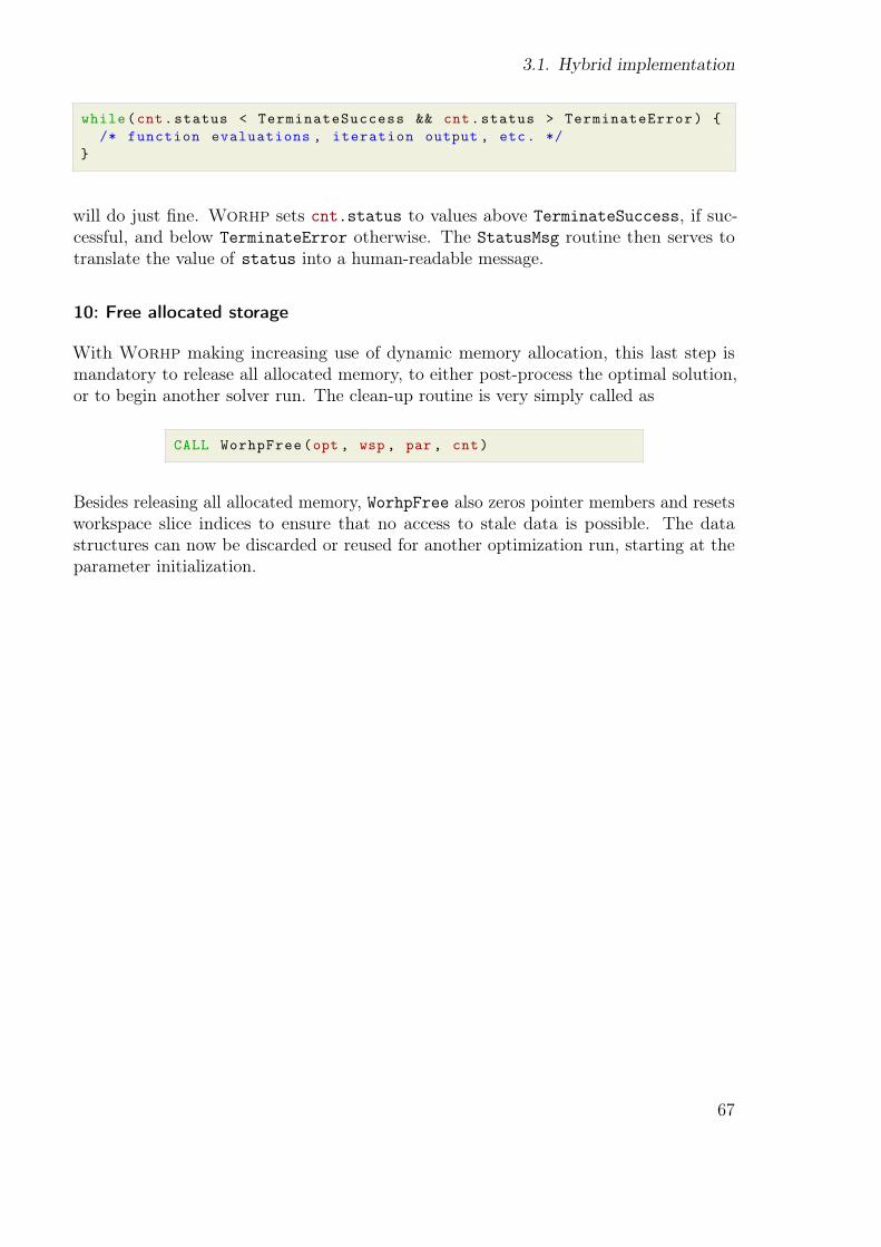
3.1. Hybrid implementation
while(cnt.status < TerminateSuccess && cnt.status > TerminateError) {
/* function evaluations , iteration output , etc. */
}
will do just őne. Worhp sets cnt.status to values above TerminateSuccess, if suc-cessful, and below TerminateError otherwise. The StatusMsg routine then serves totranslate the value of status into a human-readable message.
10: Free allocated storage
With Worhp making increasing use of dynamic memory allocation, this last step ismandatory to release all allocated memory, to either post-process the optimal solution,or to begin another solver run. The clean-up routine is very simply called as
CALL WorhpFree(opt , wsp , par , cnt)
Besides releasing all allocated memory, WorhpFree also zeros pointer members and resetsworkspace slice indices to ensure that no access to stale data is possible. The datastructures can now be discarded or reused for another optimization run, starting at theparameter initialization.
67
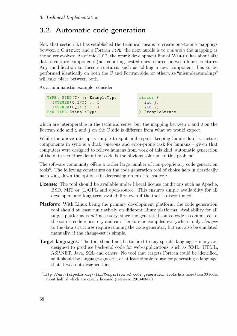
3. Technical Implementation
3.2. Automatic code generation
Now that section 3.1 has established the technical means to create one-to-one mappingsbetween a C struct and a Fortran TYPE, the next hurdle is to maintain the mapping asthe solver evolves: As of mid-2012, the trunk development line of Worhp has about 400data structure components (not counting nested ones) shared between four structures.Any modiőcation to these structures, such as adding a new component, has to beperformed identically on both the C and Fortran side, or otherwise łmisunderstandingsžwill take place between both.
As a minimalistic example, consider
TYPE , BIND(C) :: ExampleType
INTEGER(C_INT) :: I
INTEGER(C_INT) :: J
END TYPE ExampleType
struct {
int j;
int i;
} ExampleStruct
which are interoperable in the technical sense, but the mapping between I and J on theFortran side and i and j on the C side is diferent from what we would expect.
While the above mix-up is simple to spot and repair, keeping hundreds of structurecomponents in sync is a drab, onerous and error-prone task for humans ś given thatcomputers were designed to relieve humans from work of this kind, automatic generationof the data structure deőnition code is the obvious solution to this problem.
The software community ofers a rather large number of non-proprietary code generationtools6. The following constraints on the code generation tool of choice help in drasticallynarrowing down the options (in decreasing order of relevance):
License: The tool should be available under liberal license conditions such as Apache,BSD, MIT or (L)GPL and open-source. This ensures simple availability for alldevelopers and long-term availability, even if the tool is discontinued.
Platform: With Linux being the primary development platform, the code generationtool should at least run natively on diferent Linux platforms. Availability for alltarget platforms is not necessary, since the generated source-code is committed tothe source-code repository and can therefore be compiled everywhere; only changesto the data structures require running the code generator, but can also be emulatedmanually, if the change-set is simple.
Target languages: The tool should not be tailored to any speciőc language ś many aredesigned to produce back-end code for web-applications, such as XML, HTML,ASP.NET, Java, SQL and others. No tool that targets Fortran could be identiőed,so it should be language-agnostic, or at least simple to use for generating a languagethat it was not designed for.
6http://en.wikipedia.org/wiki/Comparison_of_code_generation_tools lists more than 30 tools,about half of which are openly licensed (retrieved 2013-03-08)
68

3.2. Automatic code generation
Data representation: The code generator should use a single data őle using a simplesyntax for describing the data structure components and templates for generatingthe individual C and Fortran source őles.
Extensibility: The generator tool should be easily extensible in addition to its ownfunctionality, which involves providing code snippets in the language the tool iswritten in, if it is based on an interpreted or JIT language like Python or C#.
Tool language: The tool itself should be written in a common language that is readilyavailable for Linux as primary development platform, such as C, C++, Perl, Python,. . . , or with some restrictions Java, C#, Lisp/Scheme, since these depend onadditional runtime environments.
The code generation tools GNU AutoGen[47] and cog [3] both satisfy the above require-ments.
AutoGen is written in C and uses guile[5] as Scheme interpreter, which allows seamlessextension of the inbuilt functionality through user-deőned Scheme functions. It reads asingle deőnition őle containing arbitrary key-value pairs, similar to C struct deőnitions,and template őles with AutoGen-speciőc syntax (which actually consists mostly ofScheme functions embedded in AutoGen tags) to generate output őles. AutoGen isable to generate any textual output format, depending only on the template őle, sinceit is completely language-agnostic; it does ofer some auxiliary functions that facilitategenerating C őles, though.
cog is based on Python and its design is more general than AutoGen: cog searches forspecial tags in a őle (which can have any textual format, provided it has block or linecomments) and executes the enclosed code with the Python interpreter. This makes itpossible to use cog for small, inline code generation task, but also for mimicking thebehavior of AutoGen by including a central deőnition őle in a Python-readable format.
3.2.1. Data structure definition
The current code generation for Worhp is based on AutoGen, since the concept andsyntax of the deőnition őle is closely related to the (initial) task of the code generation;in fact, the initial deőnition őle was semi-automatically generated from the existing datastructure code using sed and Perl, a task that was simpliőed by the close correlationbetween the AutoGen deőnition őle syntax and the data structure C headers.
The most important distinction made by the code generation is between basic and structi.e. derived types, and between scalars and arrays, since the initialization mechanismsdifer greatly. Basic types are double, float, int, size_t, counter, rwmt_index,iwmt_index and bool, which are translated to the corresponding types in C and Fortranthrough simple translation tables. If a component őts none of the types above, it isassumed to be a struct type; struct types are derived types, such as the WorhpMatrix
type, which have dedicated initialization and clean-up routines. Arrays may be static or
69
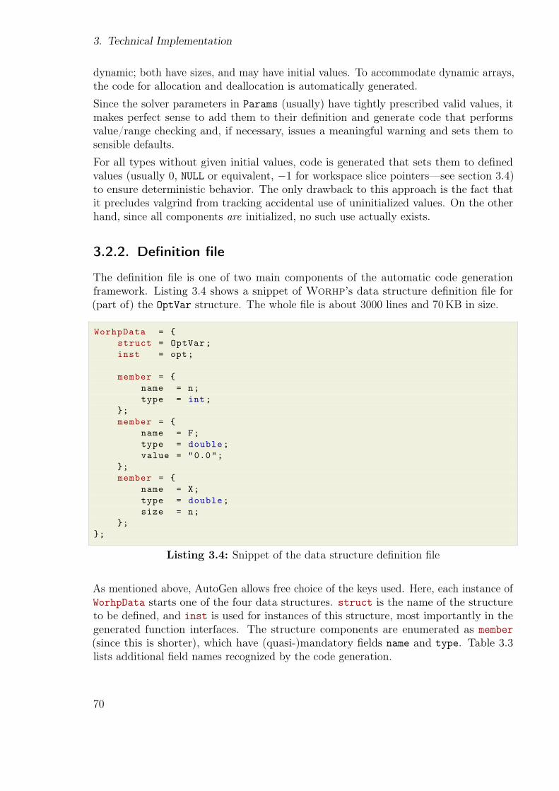
3. Technical Implementation
dynamic; both have sizes, and may have initial values. To accommodate dynamic arrays,the code for allocation and deallocation is automatically generated.
Since the solver parameters in Params (usually) have tightly prescribed valid values, itmakes perfect sense to add them to their deőnition and generate code that performsvalue/range checking and, if necessary, issues a meaningful warning and sets them tosensible defaults.
For all types without given initial values, code is generated that sets them to deőnedvalues (usually 0, NULL or equivalent, −1 for workspace slice pointersÐsee section 3.4)to ensure deterministic behavior. The only drawback to this approach is the fact thatit precludes valgrind from tracking accidental use of uninitialized values. On the otherhand, since all components are initialized, no such use actually exists.
3.2.2. Definition file
The deőnition őle is one of two main components of the automatic code generationframework. Listing 3.4 shows a snippet of Worhp’s data structure deőnition őle for(part of) the OptVar structure. The whole őle is about 3000 lines and 70KB in size.
WorhpData = {
struct = OptVar;
inst = opt;
member = {
name = n;
type = int;
};
member = {
name = F;
type = double;
value = "0.0";
};
member = {
name = X;
type = double;
size = n;
};
};
Listing 3.4: Snippet of the data structure deőnition őle
As mentioned above, AutoGen allows free choice of the keys used. Here, each instance ofWorhpData starts one of the four data structures. struct is the name of the structureto be deőned, and inst is used for instances of this structure, most importantly in thegenerated function interfaces. The structure components are enumerated as member
(since this is shorter), which have (quasi-)mandatory őelds name and type. Table 3.3lists additional őeld names recognized by the code generation.
70
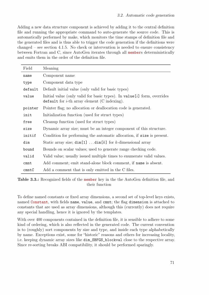
3.2. Automatic code generation
Adding a new data structure component is achieved by adding it to the central deőnitionőle and running the appropriate command to auto-generate the source code. This isautomatically performed by make, which monitors the time stamps of deőnition őle andthe generated őles and is thus able to trigger the code generation if the deőnitions werechanged ś see section 4.1.5. No check or intervention is needed to ensure consistencybetween Fortran and C, since AutoGen iterates through all members deterministicallyand emits them in the order of the deőnition őle.
Field Meaning
name Component name
type Component data type
default Default initial value (only valid for basic types)
value Initial value (only valid for basic types). In value[i] form, overridesdefault for i-th array element (C indexing).
pointer Pointer ŕag; no allocation or deallocation code is generated.
init Initialization function (used for struct types)
free Cleanup function (used for struct types)
size Dynamic array size; must be an integer component of this structure.
initif Condition for performing the automatic allocation, if size is present.
dim Static array size; dim[1] . . . dim[k] for k-dimensional array
bound Bounds on scalar values; used to generate range checking code.
valid Valid value; usually issued multiple times to enumerate valid values.
cmnt Add comment; emit stand-alone block comment, if name is absent.
cmntC Add a comment that is only emitted in the C őles.
Table 3.3.: Recognized őelds of the member key in the the AutoGen deőnition őle, andtheir function
To deőne named constants or őxed array dimensions, a second set of top-level keys exists,named Constant, with őelds name, value, and cmnt; the ŕag dimension is attached toconstants that are used as array dimensions, although this (currently) does not requireany special handling, hence it is ignored by the templates.
With over 400 components contained in the deőnition őle, it is sensible to adhere to somekind of ordering, which is also reŕected in the generated code. The current conventionis to (roughly) sort components by size and type, and inside each type alphabeticallyby name. Exceptions exist, some for łhistoricž reasons and others for increasing locality,i.e. keeping dynamic array sizes like dim_SBFGS_blockval close to the respective array.Since re-sorting breaks ABI compatibility, it should be performed sparingly.
71
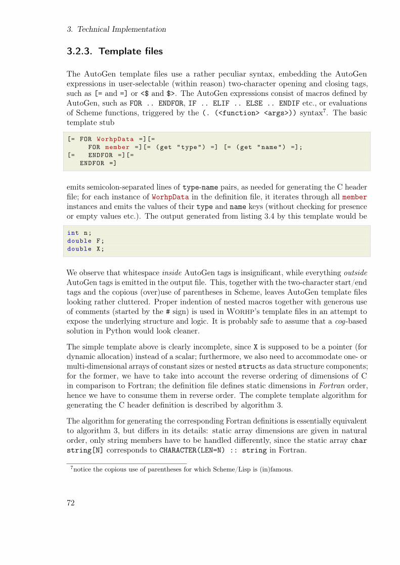
3. Technical Implementation
3.2.3. Template files
The AutoGen template őles use a rather peculiar syntax, embedding the AutoGenexpressions in user-selectable (within reason) two-character opening and closing tags,such as [= and =] or <$ and $>. The AutoGen expressions consist of macros deőned byAutoGen, such as FOR .. ENDFOR, IF .. ELIF .. ELSE .. ENDIF etc., or evaluationsof Scheme functions, triggered by the (. (<function> <args>)) syntax7. The basictemplate stub
[= FOR WorhpData =][=
FOR member =][= (get "type") =] [= (get "name") =];
[= ENDFOR =][=
ENDFOR =]
emits semicolon-separated lines of type-name pairs, as needed for generating the C headerőle; for each instance of WorhpData in the deőnition őle, it iterates through all memberinstances and emits the values of their type and name keys (without checking for presenceor empty values etc.). The output generated from listing 3.4 by this template would be
int n;
double F;
double X;
We observe that whitespace inside AutoGen tags is insigniőcant, while everything outsideAutoGen tags is emitted in the output őle. This, together with the two-character start/endtags and the copious (over)use of parentheses in Scheme, leaves AutoGen template őleslooking rather cluttered. Proper indention of nested macros together with generous useof comments (started by the # sign) is used in Worhp’s template őles in an attempt toexpose the underlying structure and logic. It is probably safe to assume that a cog-basedsolution in Python would look cleaner.
The simple template above is clearly incomplete, since X is supposed to be a pointer (fordynamic allocation) instead of a scalar; furthermore, we also need to accommodate one- ormulti-dimensional arrays of constant sizes or nested structs as data structure components;for the former, we have to take into account the reverse ordering of dimensions of Cin comparison to Fortran; the deőnition őle deőnes static dimensions in Fortran order,hence we have to consume them in reverse order. The complete template algorithm forgenerating the C header deőnition is described by algorithm 3.
The algorithm for generating the corresponding Fortran deőnitions is essentially equivalentto algorithm 3, but difers in its details: static array dimensions are given in naturalorder, only string members have to be handled diferently, since the static array char
string[N] corresponds to CHARACTER(LEN=N) :: string in Fortran.
7notice the copious use of parentheses for which Scheme/Lisp is (in)famous.
72
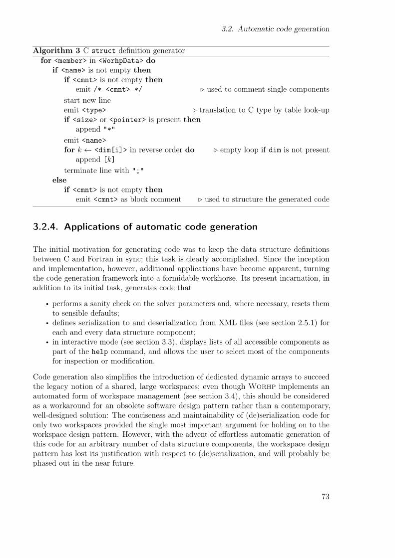
3.2. Automatic code generation
Algorithm 3 C struct deőnition generatorfor <member> in <WorhpData> do
if <name> is not empty thenif <cmnt> is not empty then
emit /* <cmnt> */ ◃ used to comment single componentsstart new lineemit <type> ◃ translation to C type by table look-upif <size> or <pointer> is present then
append "*"
emit <name>for k ← <dim[i]> in reverse order do ◃ empty loop if dim is not present
append [k]
terminate line with ";"
elseif <cmnt> is not empty then
emit <cmnt> as block comment ◃ used to structure the generated code
3.2.4. Applications of automatic code generation
The initial motivation for generating code was to keep the data structure deőnitionsbetween C and Fortran in sync; this task is clearly accomplished. Since the inceptionand implementation, however, additional applications have become apparent, turningthe code generation framework into a formidable workhorse. Its present incarnation, inaddition to its initial task, generates code that
• performs a sanity check on the solver parameters and, where necessary, resets themto sensible defaults;
• deőnes serialization to and deserialization from XML őles (see section 2.5.1) foreach and every data structure component;
• in interactive mode (see section 3.3), displays lists of all accessible components aspart of the help command, and allows the user to select most of the componentsfor inspection or modiőcation.
Code generation also simpliőes the introduction of dedicated dynamic arrays to succeedthe legacy notion of a shared, large workspaces; even though Worhp implements anautomated form of workspace management (see section 3.4), this should be consideredas a workaround for an obsolete software design pattern rather than a contemporary,well-designed solution: The conciseness and maintainability of (de)serialization code foronly two workspaces provided the single most important argument for holding on to theworkspace design pattern. However, with the advent of efortless automatic generation ofthis code for an arbitrary number of data structure components, the workspace designpattern has lost its justiőcation with respect to (de)serialization, and will probably bephased out in the near future.
73
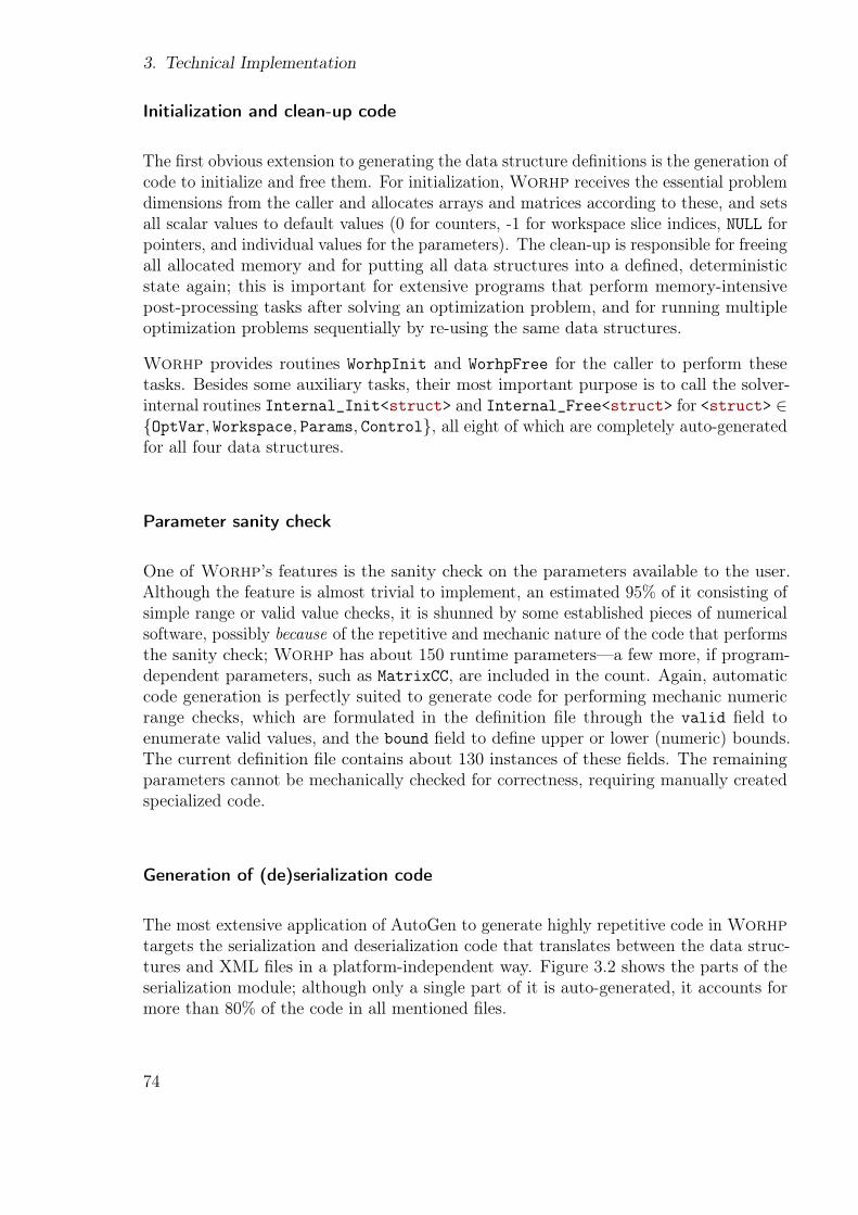
3. Technical Implementation
Initialization and clean-up code
The őrst obvious extension to generating the data structure deőnitions is the generation ofcode to initialize and free them. For initialization, Worhp receives the essential problemdimensions from the caller and allocates arrays and matrices according to these, and setsall scalar values to default values (0 for counters, -1 for workspace slice indices, NULL forpointers, and individual values for the parameters). The clean-up is responsible for freeingall allocated memory and for putting all data structures into a deőned, deterministicstate again; this is important for extensive programs that perform memory-intensivepost-processing tasks after solving an optimization problem, and for running multipleoptimization problems sequentially by re-using the same data structures.
Worhp provides routines WorhpInit and WorhpFree for the caller to perform thesetasks. Besides some auxiliary tasks, their most important purpose is to call the solver-internal routines Internal_Init<struct> and Internal_Free<struct> for <struct> ∈{OptVar, Workspace, Params, Control}, all eight of which are completely auto-generatedfor all four data structures.
Parameter sanity check
One of Worhp’s features is the sanity check on the parameters available to the user.Although the feature is almost trivial to implement, an estimated 95% of it consisting ofsimple range or valid value checks, it is shunned by some established pieces of numericalsoftware, possibly because of the repetitive and mechanic nature of the code that performsthe sanity check; Worhp has about 150 runtime parametersÐa few more, if program-dependent parameters, such as MatrixCC, are included in the count. Again, automaticcode generation is perfectly suited to generate code for performing mechanic numericrange checks, which are formulated in the deőnition őle through the valid őeld toenumerate valid values, and the bound őeld to deőne upper or lower (numeric) bounds.The current deőnition őle contains about 130 instances of these őelds. The remainingparameters cannot be mechanically checked for correctness, requiring manually createdspecialized code.
Generation of (de)serialization code
The most extensive application of AutoGen to generate highly repetitive code in Worhp
targets the serialization and deserialization code that translates between the data struc-tures and XML őles in a platform-independent way. Figure 3.2 shows the parts of theserialization module; although only a single part of it is auto-generated, it accounts formore than 80% of the code in all mentioned őles.
74
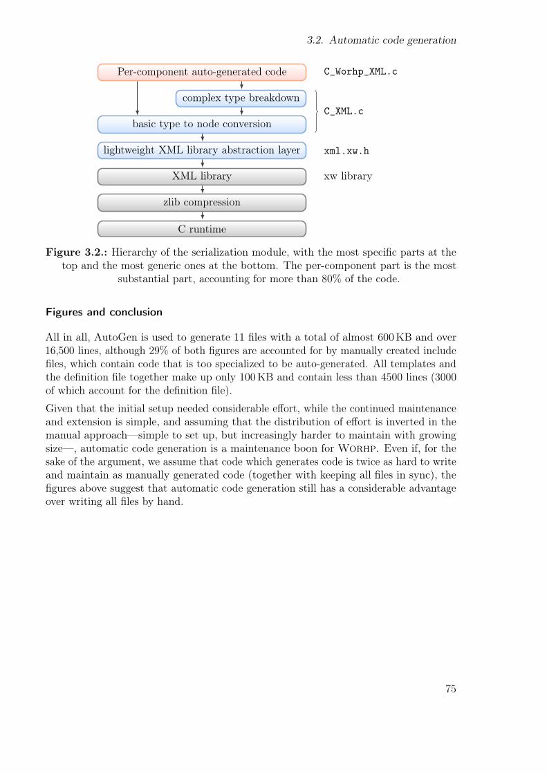
3.2. Automatic code generation
Per-component auto-generated code
complex type breakdown
basic type to node conversion
lightweight XML library abstraction layer
XML library
zlib compression
C runtime
C_Worhp_XML.c
C_XML.c
xml.xw.h
xw library
Figure 3.2.: Hierarchy of the serialization module, with the most speciőc parts at thetop and the most generic ones at the bottom. The per-component part is the most
substantial part, accounting for more than 80% of the code.
Figures and conclusion
All in all, AutoGen is used to generate 11 őles with a total of almost 600KB and over16,500 lines, although 29% of both őgures are accounted for by manually created includeőles, which contain code that is too specialized to be auto-generated. All templates andthe deőnition őle together make up only 100KB and contain less than 4500 lines (3000of which account for the deőnition őle).
Given that the initial setup needed considerable efort, while the continued maintenanceand extension is simple, and assuming that the distribution of efort is inverted in themanual approachÐsimple to set up, but increasingly harder to maintain with growingsizeÐ, automatic code generation is a maintenance boon for Worhp. Even if, for thesake of the argument, we assume that code which generates code is twice as hard to writeand maintain as manually generated code (together with keeping all őles in sync), theőgures above suggest that automatic code generation still has a considerable advantageover writing all őles by hand.
75

3. Technical Implementation
3.3. Interactive mode
The interactive mode of Worhp is motivated by the desire to be able to inŕuence (long-running) optimization runs in real time. Examples for possible runtime interventionsinclude increasing the amount of output to inspect conspicuous iteration progress, őne-tuning parameters such as MaxIter (to prevent unsuccessful termination), activating afeasibility mode, or saving the current iterate to a logőle. With traditional NLP solvers,this is either impossible to achieve, or at least requires a modiőcation of the callingprogram and a restart of the optimization run.
While Reverse Communication does in principle ofer very őne-grained control over theoptimization process, its use is limited to the calling program. Equipping it with thenecessary degree of intelligence and autonomy to react to any conceivable condition thatwould cause a human user to intervene is an unrealistic goal Ð a much more feasibleapproach is to actually enable runtime interventions: The interactive mode listens tokeyboard commands Ctrl+L and Ctrl+I.
Ctrl+L
Ctrl+I
ITER OBJ CON sKKT FLAGS TIME
[ 0| 18] -1.32300000E+01 9.87E-01 2.24E-02 Uin 4.00E-02
Worhp: Writing logfile
* Logfile written
[ 1| 119] -2.24623190E+02 1.78E+00 4.14E+02 Uin 3.60E-01
[ 2| 75] -2.23659601E+02 1.60E+00 3.22E+02 Uin 5.40E-01
(Worhp) norm opt.x
9.5461941162E+03
(Worhp) c
[ 3| 36] -2.23191095E+02 1.58E+00 8.76E+02 Uin 6.60E-01
The Ctrl+L keyboard command instructs Worhp to write the current iterate to alogőle (a partial or complete Hotstart őle, see section 2.5.1) but otherwise continuethe iteration process, while Ctrl+I pauses the optimization to present a rudimentaryprompt to the user, ofering various ways of data inspection and interaction through anumber of simple commands. Listing 3.5 shows the help-screen output of the interactivemode, enumerating the commands understood by it, and listing 3.6 shows an exemplarylisting of the components of the OptVar structure using the 1-argument form of the help
command that is intended for use as reference.
Implementation
The interactive mode is implemented through a Fortran-based parser: Each user input isassumed to consist of at most 3 tokens, separated by whitespace. The őrst (and possiblyonly) token is always a command, possibly followed by an argument (two arguments inthe set case). If the second argument is given, it is assumed to be the name of a datastructure component. The code auto-generation is used to create and maintain a list
76
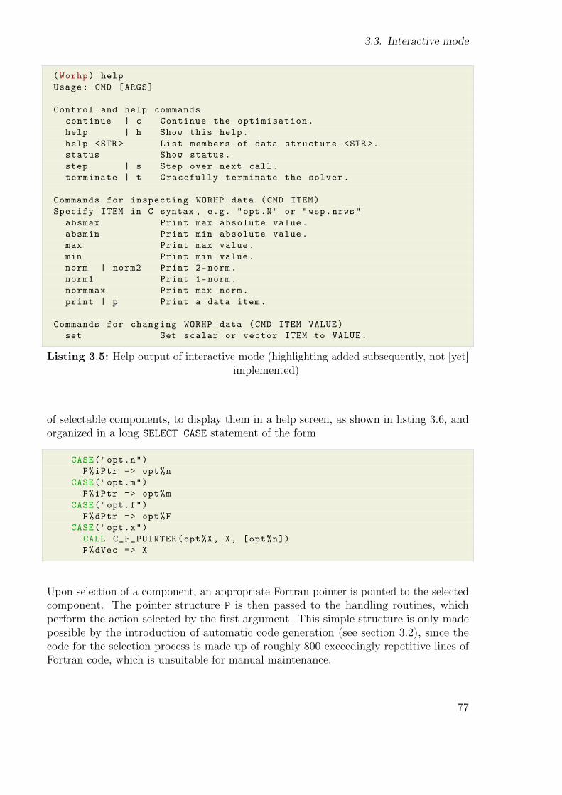
3.3. Interactive mode
(Worhp) help
Usage: CMD [ARGS]
Control and help commands
continue | c Continue the optimisation.
help | h Show this help.
help <STR > List members of data structure <STR >.
status Show status.
step | s Step over next call.
terminate | t Gracefully terminate the solver.
Commands for inspecting WORHP data (CMD ITEM)
Specify ITEM in C syntax , e.g. "opt.N" or "wsp.nrws"
absmax Print max absolute value.
absmin Print min absolute value.
max Print max value.
min Print min value.
norm | norm2 Print 2-norm.
norm1 Print 1-norm.
normmax Print max -norm.
print | p Print a data item.
Commands for changing WORHP data (CMD ITEM VALUE)
set Set scalar or vector ITEM to VALUE.
Listing 3.5: Help output of interactive mode (highlighting added subsequently, not [yet]implemented)
of selectable components, to display them in a help screen, as shown in listing 3.6, andorganized in a long SELECT CASE statement of the form
CASE("opt.n")
P%iPtr => opt%n
CASE("opt.m")
P%iPtr => opt%m
CASE("opt.f")
P%dPtr => opt%F
CASE("opt.x")
CALL C_F_POINTER(opt%X, X, [opt%n])
P%dVec => X
Upon selection of a component, an appropriate Fortran pointer is pointed to the selectedcomponent. The pointer structure P is then passed to the handling routines, whichperform the action selected by the őrst argument. This simple structure is only madepossible by the introduction of automatic code generation (see section 3.2), since thecode for the selection process is made up of roughly 800 exceedingly repetitive lines ofFortran code, which is unsuitable for manual maintenance.
77
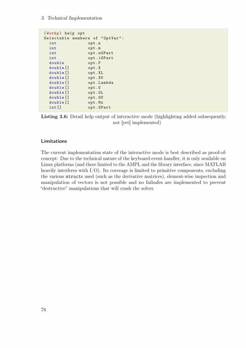
3. Technical Implementation
(Worhp) help opt
Selectable members of "OptVar":
int opt.n
int opt.m
int opt.nGPart
int opt.iGPart
double opt.F
double [] opt.X
double [] opt.XL
double [] opt.XU
double [] opt.Lambda
double [] opt.G
double [] opt.GL
double [] opt.GU
double [] opt.Mu
int[] opt.GPart
Listing 3.6: Detail help output of interactive mode (highlighting added subsequently,not [yet] implemented)
Limitations
The current implementation state of the interactive mode is best described as proof-of-concept: Due to the technical nature of the keyboard-event-handler, it is only available onLinux platforms (and there limited to the AMPL and the library interface, since MATLABheavily interferes with I/O). Its coverage is limited to primitive components, excludingthe various structs used (such as the derivative matrices), element-wise inspection andmanipulation of vectors is not possible and no failsafes are implemented to preventłdestructivež manipulations that will crash the solver.
78
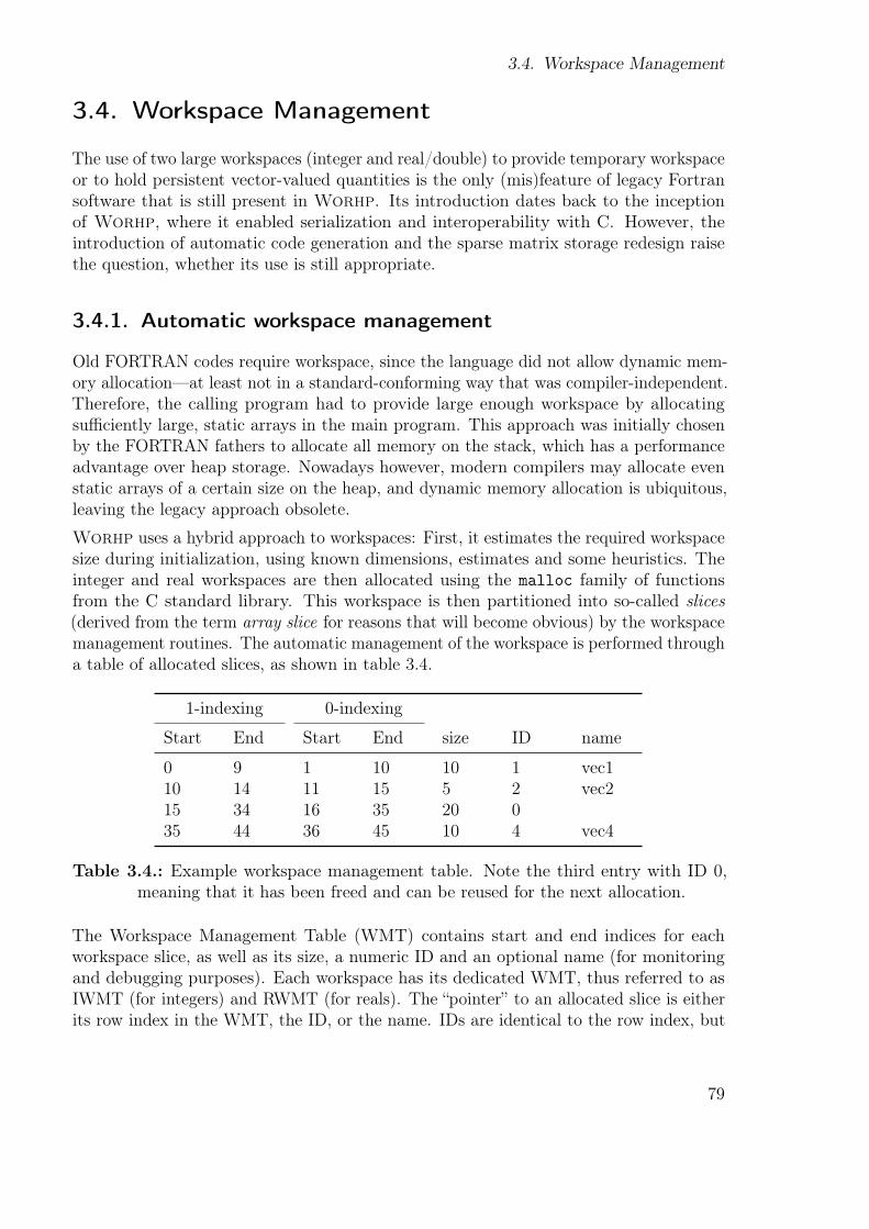
3.4. Workspace Management
3.4. Workspace Management
The use of two large workspaces (integer and real/double) to provide temporary workspaceor to hold persistent vector-valued quantities is the only (mis)feature of legacy Fortransoftware that is still present in Worhp. Its introduction dates back to the inceptionof Worhp, where it enabled serialization and interoperability with C. However, theintroduction of automatic code generation and the sparse matrix storage redesign raisethe question, whether its use is still appropriate.
3.4.1. Automatic workspace management
Old FORTRAN codes require workspace, since the language did not allow dynamic mem-ory allocationÐat least not in a standard-conforming way that was compiler-independent.Therefore, the calling program had to provide large enough workspace by allocatingsuiciently large, static arrays in the main program. This approach was initially chosenby the FORTRAN fathers to allocate all memory on the stack, which has a performanceadvantage over heap storage. Nowadays however, modern compilers may allocate evenstatic arrays of a certain size on the heap, and dynamic memory allocation is ubiquitous,leaving the legacy approach obsolete.
Worhp uses a hybrid approach to workspaces: First, it estimates the required workspacesize during initialization, using known dimensions, estimates and some heuristics. Theinteger and real workspaces are then allocated using the malloc family of functionsfrom the C standard library. This workspace is then partitioned into so-called slices(derived from the term array slice for reasons that will become obvious) by the workspacemanagement routines. The automatic management of the workspace is performed througha table of allocated slices, as shown in table 3.4.
1-indexing 0-indexing
Start End Start End size ID name
0 9 1 10 10 1 vec110 14 11 15 5 2 vec215 34 16 35 20 035 44 36 45 10 4 vec4
Table 3.4.: Example workspace management table. Note the third entry with ID 0,meaning that it has been freed and can be reused for the next allocation.
The Workspace Management Table (WMT) contains start and end indices for eachworkspace slice, as well as its size, a numeric ID and an optional name (for monitoringand debugging purposes). Each workspace has its dedicated WMT, thus referred to asIWMT (for integers) and RWMT (for reals). The łpointerž to an allocated slice is eitherits row index in the WMT, the ID, or the name. IDs are identical to the row index, but
79
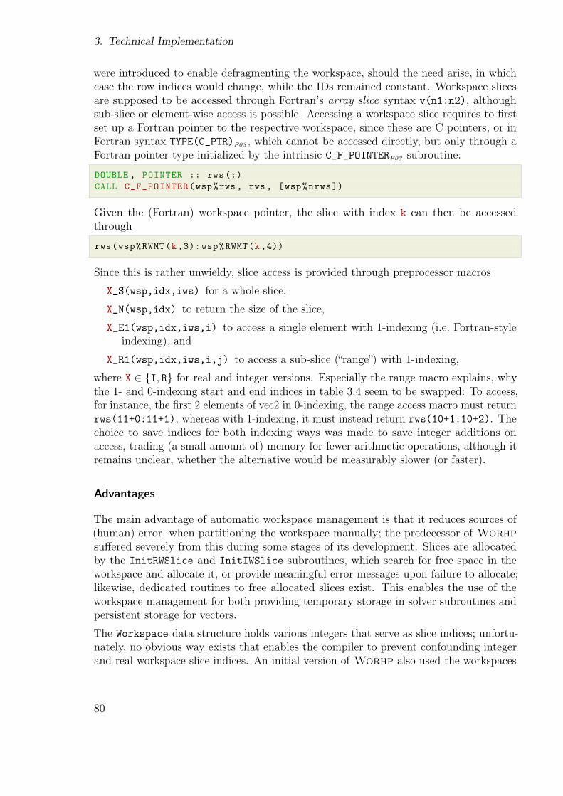
3. Technical Implementation
were introduced to enable defragmenting the workspace, should the need arise, in whichcase the row indices would change, while the IDs remained constant. Workspace slicesare supposed to be accessed through Fortran’s array slice syntax v(n1:n2), althoughsub-slice or element-wise access is possible. Accessing a workspace slice requires to őrstset up a Fortran pointer to the respective workspace, since these are C pointers, or inFortran syntax TYPE(C_PTR)F03 , which cannot be accessed directly, but only through aFortran pointer type initialized by the intrinsic C_F_POINTERF03 subroutine:
DOUBLE , POINTER :: rws (:)
CALL C_F_POINTER(wsp%rws , rws , [wsp%nrws])
Given the (Fortran) workspace pointer, the slice with index k can then be accessedthrough
rws(wsp%RWMT(k,3): wsp%RWMT(k,4))
Since this is rather unwieldy, slice access is provided through preprocessor macros
X_S(wsp,idx,iws) for a whole slice,
X_N(wsp,idx) to return the size of the slice,
X_E1(wsp,idx,iws,i) to access a single element with 1-indexing (i.e. Fortran-styleindexing), and
X_R1(wsp,idx,iws,i,j) to access a sub-slice (łrangež) with 1-indexing,
where X ∈ {I, R} for real and integer versions. Especially the range macro explains, whythe 1- and 0-indexing start and end indices in table 3.4 seem to be swapped: To access,for instance, the őrst 2 elements of vec2 in 0-indexing, the range access macro must returnrws(11+0:11+1), whereas with 1-indexing, it must instead return rws(10+1:10+2). Thechoice to save indices for both indexing ways was made to save integer additions onaccess, trading (a small amount of) memory for fewer arithmetic operations, although itremains unclear, whether the alternative would be measurably slower (or faster).
Advantages
The main advantage of automatic workspace management is that it reduces sources of(human) error, when partitioning the workspace manually; the predecessor of Worhp
sufered severely from this during some stages of its development. Slices are allocatedby the InitRWSlice and InitIWSlice subroutines, which search for free space in theworkspace and allocate it, or provide meaningful error messages upon failure to allocate;likewise, dedicated routines to free allocated slices exist. This enables the use of theworkspace management for both providing temporary storage in solver subroutines andpersistent storage for vectors.
The Workspace data structure holds various integers that serve as slice indices; unfortu-nately, no obvious way exists that enables the compiler to prevent confounding integerand real workspace slice indices. An initial version of Worhp also used the workspaces
80
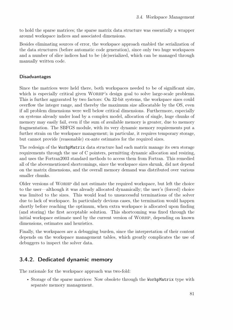
3.4. Workspace Management
to hold the sparse matrices; the sparse matrix data structure was essentially a wrapperaround workspace indices and associated dimensions.
Besides eliminating sources of error, the workspace approach enabled the serialization ofthe data structures (before automatic code generation), since only two huge workspacesand a number of slice indices had to be (de)serialized, which can be managed throughmanually written code.
Disadvantages
Since the matrices were held there, both workspaces needed to be of signiőcant size,which is especially critical given Worhp’s design goal to solve large-scale problems.This is further aggravated by two factors: On 32-bit systems, the workspace sizes couldoverŕow the integer range, and thereby the maximum size allocatable by the OS, evenif all problem dimensions were well below critical dimensions. Furthermore, especiallyon systems already under load by a complex model, allocation of single, huge chunks ofmemory may easily fail, even if the sum of available memory is greater, due to memoryfragmentation. The SBFGS module, with its very dynamic memory requirements put afurther strain on the workspace management; in particular, it requires temporary storage,but cannot provide (reasonable) ex-ante estimates for the required sizes.
The redesign of the WorhpMatrix data structure had each matrix manage its own storagerequirements through the use of C pointers, permitting dynamic allocation and resizing,and uses the Fortran2003 standard methods to access them from Fortran. This remediedall of the abovementioned shortcomings, since the workspace sizes shrunk, did not dependon the matrix dimensions, and the overall memory demand was distributed over varioussmaller chunks.
Older versions of Worhp did not estimate the required workspace, but left the choiceto the userÐalthough it was already allocated dynamically; the user’s (forced) choicewas limited to the sizes. This would lead to unsuccessful terminations of the solverdue to lack of workspace. In particularly devious cases, the termination would happenshortly before reaching the optimum, when extra workspace is allocated upon őnding(and storing) the őrst acceptable solution. This shortcoming was őxed through theinitial workspace estimate used by the current version of Worhp, depending on knowndimensions, estimates and heuristics.
Finally, the workspaces are a debugging burden, since the interpretation of their contentdepends on the workspace management tables, which greatly complicates the use ofdebuggers to inspect the solver data.
3.4.2. Dedicated dynamic memory
The rationale for the workspace approach was two-fold:
• Storage of the sparse matrices: Now obsolete through the WorhpMatrix type withseparate memory management.
81
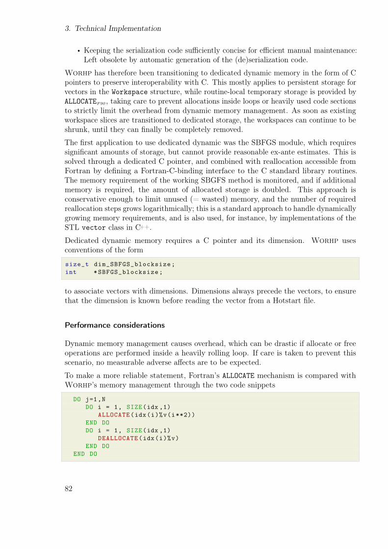
3. Technical Implementation
• Keeping the serialization code suiciently concise for eicient manual maintenance:Left obsolete by automatic generation of the (de)serialization code.
Worhp has therefore been transitioning to dedicated dynamic memory in the form of Cpointers to preserve interoperability with C. This mostly applies to persistent storage forvectors in the Workspace structure, while routine-local temporary storage is provided byALLOCATEF90 , taking care to prevent allocations inside loops or heavily used code sectionsto strictly limit the overhead from dynamic memory management. As soon as existingworkspace slices are transitioned to dedicated storage, the workspaces can continue to beshrunk, until they can őnally be completely removed.
The őrst application to use dedicated dynamic was the SBFGS module, which requiressigniőcant amounts of storage, but cannot provide reasonable ex-ante estimates. This issolved through a dedicated C pointer, and combined with reallocation accessible fromFortran by deőning a Fortran-C-binding interface to the C standard library routines.The memory requirement of the working SBGFS method is monitored, and if additionalmemory is required, the amount of allocated storage is doubled. This approach isconservative enough to limit unused (= wasted) memory, and the number of requiredreallocation steps grows logarithmically; this is a standard approach to handle dynamicallygrowing memory requirements, and is also used, for instance, by implementations of theSTL vector class in C++.
Dedicated dynamic memory requires a C pointer and its dimension. Worhp usesconventions of the form
size_t dim_SBFGS_blocksize;
int *SBFGS_blocksize;
to associate vectors with dimensions. Dimensions always precede the vectors, to ensurethat the dimension is known before reading the vector from a Hotstart őle.
Performance considerations
Dynamic memory management causes overhead, which can be drastic if allocate or freeoperations are performed inside a heavily rolling loop. If care is taken to prevent thisscenario, no measurable adverse afects are to be expected.
To make a more reliable statement, Fortran’s ALLOCATE mechanism is compared withWorhp’s memory management through the two code snippets
DO j=1,N
DO i = 1, SIZE(idx ,1)
ALLOCATE(idx(i)%v(i**2))
END DO
DO i = 1, SIZE(idx ,1)
DEALLOCATE(idx(i)%v)
END DO
END DO
82
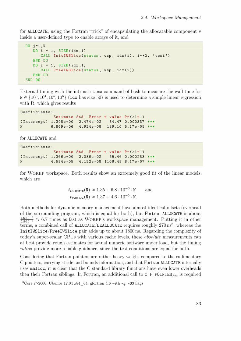
3.4. Workspace Management
for ALLOCATE, using the Fortran łtrickž of encapsulating the allocatable component v
inside a user-deőned type to enable arrays of it, and
DO j=1,N
DO i = 1, SIZE(idx ,1)
CALL InitIWSlice(status , wsp , idx(i), i**2, ’test’)
END DO
DO i = 1, SIZE(idx ,1)
CALL FreeIWSlice(status , wsp , idx(i))
END DO
END DO
External timing with the intrinsic time command of bash to measure the wall time forN ∈ {103, 104, 105, 106} (idx has size 50) is used to determine a simple linear regressionwith R, which gives results
Coefficients:
Estimate Std. Error t value Pr(>|t|)
(Intercept) 1.348e+00 2.474e-02 54.47 0.000337 ***
N 6.849e-06 4.924e-08 139.10 5.17e-05 ***
for ALLOCATE and
Coefficients:
Estimate Std. Error t value Pr(>|t|)
(Intercept) 1.366e+00 2.086e-02 65.46 0.000233 ***
N 4.594e-05 4.152e-08 1106.49 8.17e-07 ***
for Worhp workspace. Both results show an extremely good őt of the linear models,which are
tALLOCATE(N) ≈ 1.35 + 6.8 · 10−6 · N and
tIWSlice(N) ≈ 1.37 + 4.6 · 10−5 · N.
Both methods for dynamic memory management have almost identical ofsets (overheadof the surrounding program, which is equal for both), but Fortran ALLOCATE is about4.6·10−5
6.8·10−6 ≈ 6.7 times as fast as Worhp’s workspace management. Putting it in otherterms, a combined call of ALLOCATE/DEALLOCATE requires roughly 270 ns8, whereas theInitIWSlice/FreeIWSlice pair adds up to about 1800 ns. Regarding the complexity oftoday’s super-scalar CPUs with various cache levels, these absolute measurements canat best provide rough estimates for actual numeric software under load, but the timingratios provide more reliable guidance, since the test conditions are equal for both.
Considering that Fortran pointers are rather heavy-weight compared to the rudimentaryC pointers, carrying stride and bounds information, and that Fortran ALLOCATE internallyuses malloc, it is clear that the C standard library functions have even lower overheadsthen their Fortran siblings. In Fortran, an additional call to C_F_POINTERF03 is required
8Core i7-2600, Ubuntu 12.04 x84_64, gfortran 4.6 with -g -O3 flags
83
3. Technical Implementation
to access both the Worhp workspace and the dedicated dynamic memory, which causessome additional overhead. Measurements using the callgrind tool of valgrind indicate,however, that C_F_POINTER calls are rather light-weight, requiring 63 instructions and8.7 ns per call to dynamic libgfortran, and 55 instruction and 6.8 ns per call to thestatic version.
Conclusion
The use of workspaces, along with the access macros to keep the code concise, andautomatic workspace management through tables to eliminate sources of (human) errorwas an appropriate solution to enable serialization and reasonably dynamic memorymanagement. The workspace approach carries with it various disadvantages, some ofwhich afect Worhp’s performance as solver for large-scale optimization problems. Withthe redesign to workspace-independent sparse matrix structures and the introductionof automatic code generation for serialization, the workspace approach is left withoutobvious advantages, and a technically feasible alternative exists in the form of dedicateddynamic memory. Since the latter also has a performance edge over Worhp’s memorymanagement through WMTs, the only reasonable conclusion is to phase out the legacyworkspace approach, and replace it by dedicated storage. The question whether toperform this as sudden, disruptive replacement, or a slow, incremental one can only beanswered in consideration of the currently active developments.
84
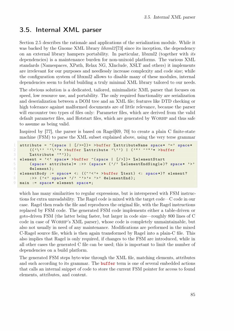
3.5. Internal XML parser
3.5. Internal XML parser
Section 2.5 describes the rationale and applications of the serialization module. While itwas backed by the Gnome XML library libxml2 [73] since its inception, the dependencyon an external library hampers portability. In particular, libxml2 (together with itsdependencies) is a maintenance burden for non-unixoid platforms. The various XMLstandards (Namespaces, XPath, Relax NG, XInclude, XSLT and others) it implementsare irrelevant for our purposes and needlessly increase complexity and code size; whilethe conőguration system of libxml2 allows to disable many of these modules, internaldependencies seem to forbid building a truly minimal XML library tailored to our needs.
The obvious solution is a dedicated, tailored, minimalistic XML parser that focuses onspeed, low resource use, and portability. The only required functionality are serializationand deserialization between a DOM tree and an XML őle; features like DTD checking orhigh tolerance against malformed documents are of little relevance, because the parserwill encounter two types of őles only: Parameter őles, which are derived from the validdefault parameter őles, and Hotstart őles, which are generated by Worhp and thus safeto assume as being valid.
Inspired by [77], the parser is based on Ragel[69, 70] to create a plain C őnite-statemachine (FSM) to parse the XML subset explained above, using the very terse grammar
1 attribute = ^(space | [/ >=])+ >buffer %attributeName space* ’=’ space*
2 ((’\’’ ^’\’’* >buffer %attribute ’\’’) | (’"’ ^’"’* >buffer
3 %attribute ’"’));
4 element = ’<’ space* >buffer ^( space | [/ >])+ %elementStart
5 (space+ attribute )* :>> (space* (’/’ %elementEndSingle )? space* ’>’
6 @element );
7 elementBody := space* <: ((^’<’+ >buffer %text) <: space *)? element?
8 :>> (’<’ space* ’/’ ^’>’+ ’>’ @elementEnd );
9 main := space* element space*;
which has many similarities to regular expressions, but is interspersed with FSM instruc-tions for extra unreadability. The Ragel code is mixed with the target codeÐC code in ourcase. Ragel then reads the őle and reproduces the original őle, with the Ragel instructionsreplaced by FSM code. The generated FSM code implements either a table-driven orgoto-driven FSM (the latter being faster, but larger in code sizeÐroughly 800 lines of Ccode in case of Worhp’s XML parser), whose code is completely unmaintainable, butalso not usually in need of any maintenance. Modiőcations are performed in the mixedC-Ragel source őle, which is then again transformed by Ragel into a plain-C őle. Thisalso implies that Ragel is only required, if changes to the FSM are introduced, while inall other cases the generated C őle can be used; this is important to limit the number ofdependencies on a build platform.
The generated FSM steps byte-wise through the XML őle, matching elements, attributesand such according to its grammar. The buffer term is one of several embedded actionsthat calls an internal snippet of code to store the current FSM pointer for access to foundelements, attributes, and content.
85
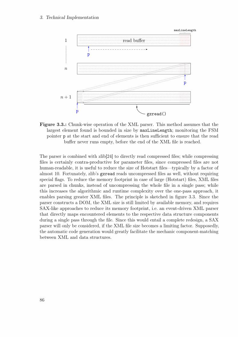
3. Technical Implementation
10101010101010101010101010101010101010101010101010101010101010101010101010101
1010101010101010101010101010101010101010101010101010101010101010101010101010
0101010101010101010101010101010101010101010101010101010101010101010101010101
maxLineLength
read bufer
p
n0101010101010101010101010101010101010101010101010101010101010101010101010101
1010101010101010101010101010101010101010101010101010101010101010101010101010
0101010101010101010101010101010101010101010101010101010101010101010101010101
p
n+ 10101010101010101010101010101010101010101010101010101010101010101010101010
1010101010101010101010101010101010101010101010101010101010101010101010101
0101010101010101010101010101010101010101010101010101010101010101010101010
101
010
101
gzread()p
Figure 3.3.: Chunk-wise operation of the XML parser. This method assumes that thelargest element found is bounded in size by maxLineLength; monitoring the FSMpointer p at the start and end of elements is then suicient to ensure that the read
bufer never runs empty, before the end of the XML őle is reached.
The parser is combined with zlib[24] to directly read compressed őles; while compressingőles is certainly contra-productive for parameter őles, since compressed őles are nothuman-readable, it is useful to reduce the size of Hotstart őlesÐtypically by a factor ofalmost 10. Fortunately, zlib’s gzread reads uncompressed őles as well, without requiringspecial ŕags. To reduce the memory footprint in case of large (Hotstart) őles, XML őlesare parsed in chunks, instead of uncompressing the whole őle in a single pass; whilethis increases the algorithmic and runtime complexity over the one-pass approach, itenables parsing greater XML őles. The principle is sketched in őgure 3.3. Since theparser constructs a DOM, the XML size is still limited by available memory, and requiresSAX-like approaches to reduce its memory footprint, i.e. an event-driven XML parserthat directly maps encountered elements to the respective data structure componentsduring a single pass through the őle. Since this would entail a complete redesign, a SAXparser will only be considered, if the XML őle size becomes a limiting factor. Supposedly,the automatic code generation would greatly facilitate the mechanic component-matchingbetween XML and data structures.
86
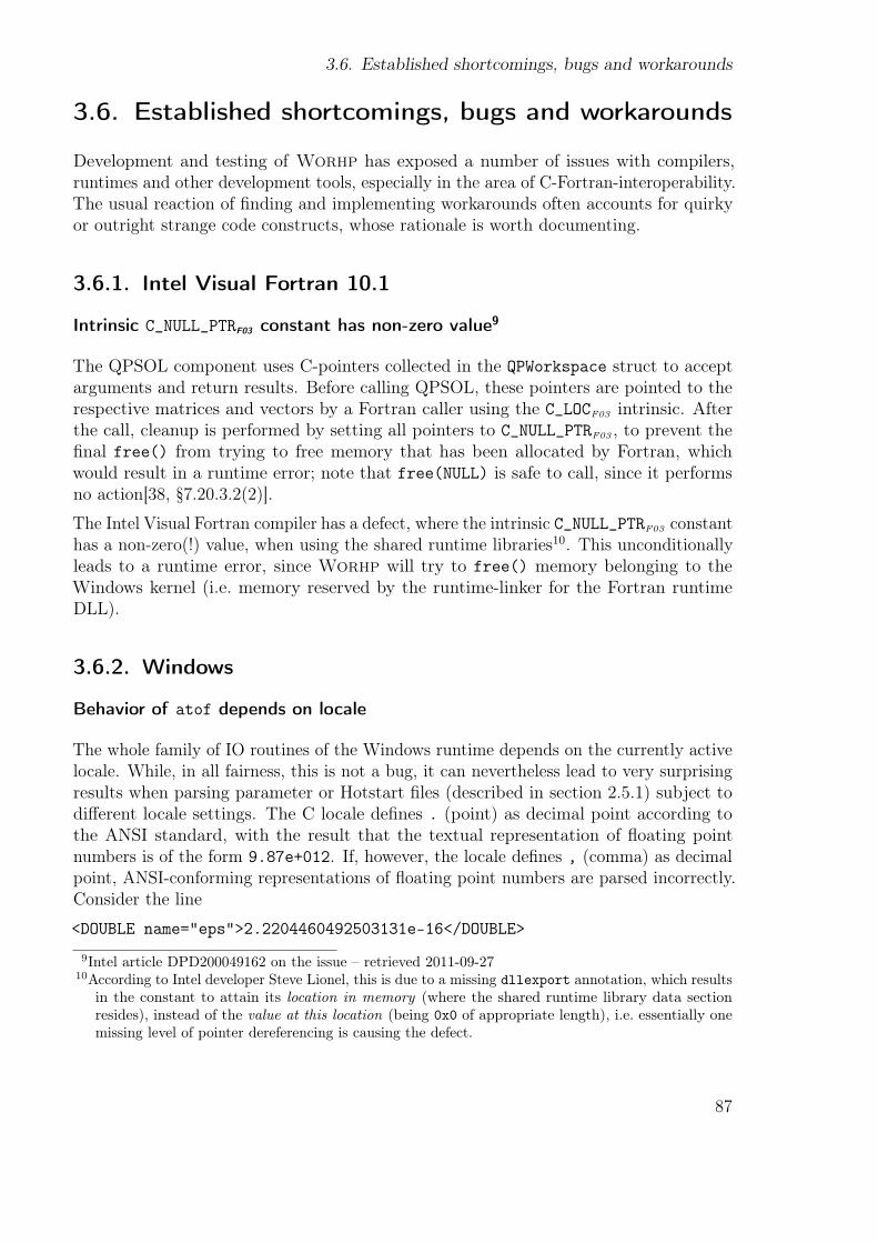
3.6. Established shortcomings, bugs and workarounds
3.6. Established shortcomings, bugs and workarounds
Development and testing of Worhp has exposed a number of issues with compilers,runtimes and other development tools, especially in the area of C-Fortran-interoperability.The usual reaction of őnding and implementing workarounds often accounts for quirkyor outright strange code constructs, whose rationale is worth documenting.
3.6.1. Intel Visual Fortran 10.1
Intrinsic C_NULL_PTRF03 constant has non-zero value9
The QPSOL component uses C-pointers collected in the QPWorkspace struct to acceptarguments and return results. Before calling QPSOL, these pointers are pointed to therespective matrices and vectors by a Fortran caller using the C_LOCF03 intrinsic. Afterthe call, cleanup is performed by setting all pointers to C_NULL_PTRF03 , to prevent theőnal free() from trying to free memory that has been allocated by Fortran, whichwould result in a runtime error; note that free(NULL) is safe to call, since it performsno action[38, ğ7.20.3.2(2)].
The Intel Visual Fortran compiler has a defect, where the intrinsic C_NULL_PTRF03 constanthas a non-zero(!) value, when using the shared runtime libraries10. This unconditionallyleads to a runtime error, since Worhp will try to free() memory belonging to theWindows kernel (i.e. memory reserved by the runtime-linker for the Fortran runtimeDLL).
3.6.2. Windows
Behavior of atof depends on locale
The whole family of IO routines of the Windows runtime depends on the currently activelocale. While, in all fairness, this is not a bug, it can nevertheless lead to very surprisingresults when parsing parameter or Hotstart őles (described in section 2.5.1) subject todiferent locale settings. The C locale deőnes . (point) as decimal point according tothe ANSI standard, with the result that the textual representation of ŕoating pointnumbers is of the form 9.87e+012. If, however, the locale deőnes , (comma) as decimalpoint, ANSI-conforming representations of ŕoating point numbers are parsed incorrectly.Consider the line
<DOUBLE name="eps">2.2204460492503131e-16</DOUBLE>
9Intel article DPD200049162 on the issue – retrieved 2011-09-2710According to Intel developer Steve Lionel, this is due to a missing dllexport annotation, which results
in the constant to attain its location in memory (where the shared runtime library data sectionresides), instead of the value at this location (being 0x0 of appropriate length), i.e. essentially onemissing level of pointer dereferencing is causing the defect.
87

3. Technical Implementation
from Worhp’s parameter őle. This deőnes the quantity to be used as machine epsilon,which is mainly needed for comparisons. On a Windows system with active German (orsimilar) locale, , (comma) is used as decimal point, hence atof parses the 2 and discardsthe rest, in particular the exponent, resulting in eps = 2 and rather odd behavior ofWorhp.
Workarounds exist:
• Retrieve the currently active decimal point by using localeconf, and if unequalto . (point), convert all number representations in ANSI form to the current localeby replacing . by the localized decimal point before handing them over to atof.
• Change the locale settings of the operating system. This is problematic, since onlyfew users will be able to, be it through lack of administrative rights or lack ofknowledge. This can also be quite disruptive to the workŕow and is therefore notrecommended.
• Use setlocale(LC_NUMERIC, "") to reset the locale settings for number represen-tations (back to ANSI). This may have an impact on the calling program, though,depending on the operating system.
88
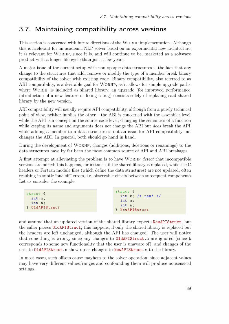
3.7. Maintaining compatibility across versions
3.7. Maintaining compatibility across versions
This section is concerned with future directions of the Worhp implementation. Althoughthis is irrelevant for an academic NLP solver based on an experimental new architecture,it is relevant for Worhp, since it is, and will continue to be, marketed as a softwareproduct with a longer life cycle than just a few years.
A major issue of the current setup with non-opaque data structures is the fact that anychange to the structures that add, remove or modify the type of a member break binarycompatibility of the solver with existing code. Binary compatibility, also referred to asABI compatibility, is a desirable goal for Worhp, as it allows for simple upgrade paths:where Worhp is included as shared library, an upgrade (for improved performance,introduction of a new feature or őxing a bug) consists solely of replacing said sharedlibrary by the new version.
ABI compatibility will usually require API compatibility, although from a purely technicalpoint of view, neither implies the other ś the ABI is concerned with the assembler level,while the API is a concept on the source code level; changing the semantics of a functionwhile keeping its name and arguments does not change the ABI but does break the API,while adding a member to a data structure is not an issue for API compatibility butchanges the ABI. In general, both should go hand in hand.
During the development of Worhp, changes (additions, deletions or renamings) to thedata structures have by far been the most common source of API and ABI breakages.
A őrst attempt at alleviating the problem is to have Worhp detect that incompatibleversions are mixed; this happens, for instance, if the shared library is replaced, while the Cheaders or Fortran module őles (which deőne the data structures) are not updated, oftenresulting in subtle łone-ofž-errors, i.e. observable ofsets between subsequent components.Let us consider the example
struct {
int m;
int n;
} OldAPIStruct
struct {
int k; /* new! */
int m;
int n;
} NewAPIStruct
and assume that an updated version of the shared library expects NewAPIStruct, butthe caller passes OldAPIStruct; this happens, if only the shared library is replaced butthe headers are left unchanged, although the API has changed. The user will noticethat something is wrong, since any changes to OldAPIStruct.m are ignored (since k
corresponds to some new functionality that the user is unaware of), and changes of theuser to OldAPIStruct.n show up as changes to NewAPIStruct.m to the library.
In most cases, such ofsets cause mayhem to the solver operation, since adjacent valuesmay have very diferent values/ranges and confounding them will produce nonsensicalsettings.
89
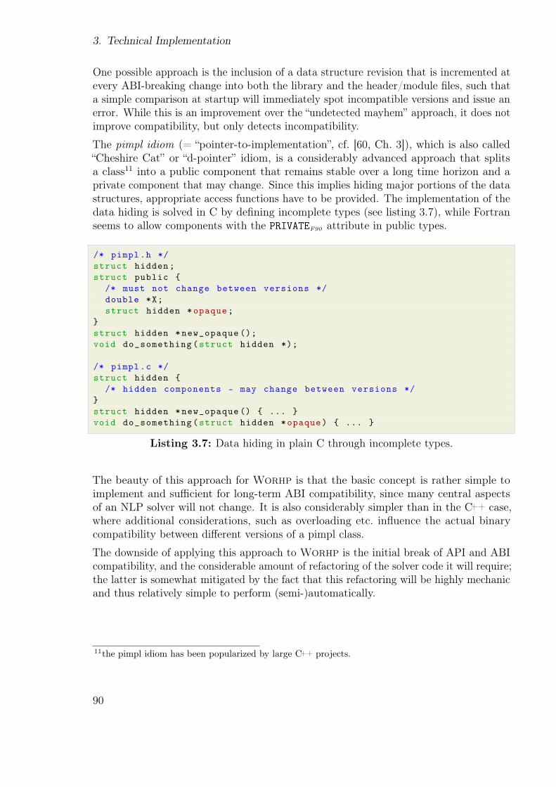
3. Technical Implementation
One possible approach is the inclusion of a data structure revision that is incremented atevery ABI-breaking change into both the library and the header/module őles, such thata simple comparison at startup will immediately spot incompatible versions and issue anerror. While this is an improvement over the łundetected mayhemž approach, it does notimprove compatibility, but only detects incompatibility.
The pimpl idiom (= łpointer-to-implementationž, cf. [60, Ch. 3]), which is also calledłCheshire Catž or łd-pointerž idiom, is a considerably advanced approach that splitsa class11 into a public component that remains stable over a long time horizon and aprivate component that may change. Since this implies hiding major portions of the datastructures, appropriate access functions have to be provided. The implementation of thedata hiding is solved in C by deőning incomplete types (see listing 3.7), while Fortranseems to allow components with the PRIVATEF90 attribute in public types.
/* pimpl.h */
struct hidden;
struct public {
/* must not change between versions */
double *X;
struct hidden *opaque;
}
struct hidden *new_opaque ();
void do_something(struct hidden *);
/* pimpl.c */
struct hidden {
/* hidden components - may change between versions */
}
struct hidden *new_opaque () { ... }
void do_something(struct hidden *opaque) { ... }
Listing 3.7: Data hiding in plain C through incomplete types.
The beauty of this approach for Worhp is that the basic concept is rather simple toimplement and suicient for long-term ABI compatibility, since many central aspectsof an NLP solver will not change. It is also considerably simpler than in the C++ case,where additional considerations, such as overloading etc. inŕuence the actual binarycompatibility between diferent versions of a pimpl class.
The downside of applying this approach to Worhp is the initial break of API and ABIcompatibility, and the considerable amount of refactoring of the solver code it will require;the latter is somewhat mitigated by the fact that this refactoring will be highly mechanicand thus relatively simple to perform (semi-)automatically.
11the pimpl idiom has been popularized by large C++ projects.
90
Chapter4
Solver Infrastructure
Wenn der Reiter nichts taugt, ist das Pferd schuld.A bad workman blames his tools.
(Proverb)
4.1. Configuration and Build system . . . . . . . . . . . . . . . . . . . 92
4.1.1. Available build tools . . . . . . . . . . . . . . . . . . . . . 92
4.1.2. Basics of make . . . . . . . . . . . . . . . . . . . . . . . . 94
4.1.3. Directory structure . . . . . . . . . . . . . . . . . . . . . . 95
4.1.4. Pitfalls of recursive make . . . . . . . . . . . . . . . . . . 96
4.1.5. Non-recursive make . . . . . . . . . . . . . . . . . . . . . 99
4.2. Version and configuration info . . . . . . . . . . . . . . . . . . . . 104
4.3. Testing Approach . . . . . . . . . . . . . . . . . . . . . . . . . . 107
4.4. Testing Infrastructure . . . . . . . . . . . . . . . . . . . . . . . . 110
4.4.1. Parallel testing script . . . . . . . . . . . . . . . . . . . . . 110
4.4.2. Solver output processing . . . . . . . . . . . . . . . . . . . 113
4.5. Parameter Tuning . . . . . . . . . . . . . . . . . . . . . . . . . . 116
4.5.1. Why tune solver parameters? . . . . . . . . . . . . . . . . 116
4.5.2. Sweeping the Parameter Space . . . . . . . . . . . . . . . 117
4.5.3. Examples . . . . . . . . . . . . . . . . . . . . . . . . . . . 120
4.5.4. Conclusions . . . . . . . . . . . . . . . . . . . . . . . . . 127
4.6. Future directions for testing . . . . . . . . . . . . . . . . . . . . . 128
91
4. Solver Infrastructure
4.1. Configuration and Build system
The conőguration and build system of Worhp is used to build the available interfaces forits supported platforms with the chosen solver conőguration. One of the most importanttasks of a build system is to track all inter-dependencies of source and conőguration őles,on the one hand to prevent unnecessary recompilation or regeneration of objects, whosedependencies have not changed, and on the other hand, to reliably trigger the necessaryrecompilation or regeneration of objects whose dependencies have changed. Failure toachieve the őrst task typically leads to time-consuming recompilation cascades, whilefailure to achieve the latter will result in incomplete or faulty builds.
The solver conőguration options to build Worhp include
• the choice of a target platform/compiler pair and system paths,• debug versus release builds (compiler optimization options),• enabling additional debug output for some solver components,• static versus shared libraries,• linear algebra solver support,• enabling optional modules (XML, licensing).
As of late 2010, Worhp is supported on these platforms
Linux: Debian, Redhat and their derivatives,
Unix: Solaris and OpenSolaris,
Mac: using MacPorts[4],
Windows: Server 2000, XP and later,
using the GNU, Intel and Microsoft compilers. Combined with the fact that Worhp
is being developed and tested on a number of systems with diferent compiler/bitnessconstellations, this leads to a large number of diferent possible conőgurations to buildthe solver. Together with the need to direct the automatic code generation and handlethe mixed-language approach, creating and maintaining the build system for Worhp isa complex task.
4.1.1. Available build tools
The development of Worhp being Linux-centric, GNU make[68] is used as the mainbuild infrastructure, since it is ubiquitous on all unixoid platforms and also available forthe other supported platforms.
Possible alternatives to GNU make are
Boost.Build: Boost.Build[1] is a Jam-based build system to conőgure and build C++
libraries or applications for various platforms. It reads concise Jamfiles that arewritten in łJamž, which has a close resemblance to make’s syntax.
92
4.1. Configuration and Build system
Since Boost.Build is C++ centric, building libraries of non-C++ sources is onlypossible by some degree of hacking, for instance by writing explicit rules for all non-C++ source őles; this, however, defeats the purpose of conciseness by automation,and introduces unwanted complexity. Also, in contrast to SCons and CMake,Boost.Build cannot resolve Fortran module dependencies.
The GNU Build System: Also being referred to as łAutotoolsž, the GNU Build Systemis a standard infrastructure component used to build most unixoid open-sourcesoftware. While the complete build system actually consists of a number of in-terlocking pieces of software, namely GNU Autoconf[18], GNU Automake[2] andoptionally GNU Autoheader (part of Autoconf) and GNU libtool[72], Autoconf issometimes used synonymously for the complete build system.
The GNU Build System constructs a portable configure script that in turninstantiates a (mostly recursive) makeőle hierarchy to build a software packageon very diferent systems. The capabilities of the configure script include cross-compiling (although this is involved), checking compiler capabilities, and detectingand working around quirks, known bugs or missing features. Projects that usethe GNU Build System are conőgured, built, and installed using the three famouscommands
./ configure
make
make install
The strength of the generated configure script lies in the fact that it performsvery őne-grained checks for actual capabilities of the build environment, insteadof relying on version look-ups or databases. A capability is tested by spawning asub-process, which runs a shell-script, compiles a small piece of test code, or runs asystem tool to inspect its output. This greatly eases porting an application, oncethe initial efort of setting of Autoconf has been sufered.
However, Autoconf has a number of serious issues:
• Autoconf is complex and has a very steep learning curve, partly due to thefact that it is built on M4, the GNU macro processor.
• The Autotools are notorious for subtle incompatibilities between their manydiferent versions, which is a burden when manipulating the build system ofmore than one project, since this may require parallel installations of diferentAutotool versions.
• Many software packages that depend on Autoconf use recursive invocationsof make. This is harmful for dependency tracking between diferent sourcedirectories, as described in 4.1.4.
• Autoconf is slow1. Part of this performance issue is caused by the repeatedspawning of sub-processes, which is a cheap operation on unixoid systems
1See e.g. section 2.7.2 (test with many dependencies) at http://retropaganda.info/~bohan/work/psycle/branches/bohan/wonderbuild/benchmarks/time.xml#2.7.2 – retrieved 2013-01-30.
93
4. Solver Infrastructure
(internally using fork), but a very costly operation e.g. on Windows platforms.Although the configure script does cache some of its results, in practicemany of the testing operations are performed repeatedly by sub-makes, andnot cached for other configure scripts by default, unless instructed so by theuser.
CMake: CMake[33], the łCross Platform Makež is a mature and powerful tool to generatebuild files to be used by the respective native build system, i.e. makeőles for unixoidsystem and Visual Studio project őles for Windows. CMake has őrst-class support forFortran 902 and claims to have facilities for tracking Fortran module dependencies.
SCons: SCons[46] is a software construction tool written in Python for C/C++, Fortranand other languages. Its power lies in the fact that its conőguration őles arealso written in Python, thus enabling the developer to use a genuine full-featuredprogramming language to tackle the build process. SCons provides a scanner for For-tran 90 (and later) őles that parses USE statements and uses string transformationsto track module dependencies.
Many less well-known build tools exist, such as waf (used by Cisco, and to build Sambaor Node.js), wonderbuild (obscure) or ninja (used to build Google Chrome), but seeingthat Worhp already requires various more or less exotic dependencies, choosing fromestablished build tools is probably wise. Despite the Fortran module dependency trackingfacilities of SCons and CMake, Worhp has thus been relying on make with manuallycreated and maintained makeőles to prevent burdening developers with further softwareand language dependencies. While this approach arguably ofers a lesser degree ofautomation, it allows much őner control of the details of the build process, which isespecially useful given the degree of complexity caused by automatic code generationand the mixed-language approach.
4.1.2. Basics of make
GNU make and other versions are controlled by writing makefiles that specify rulesconsisting of targets and their prerequisite, and recipes to specify the commands toexecute. make is completely string-based (so dir and dir/ are regarded as two diferententities) and has uncommon semantics for variable expansion. Dependencies in make areformulated as targets : prerequisites pairs, for instance foo.o : foo.c foo.h.All dependencies are condensed into a single directed acyclic graph (DAG), whose nodescorrespond to targets and prerequisites and whose edges are the dependencies imposedby rules. It is useful to note that not every DAG is a tree, because multiple targets mayshare a prerequisite (expressed in tree terminology, one child may have more than oneparent), but every tree is a DAG.
It is obviously problematic if the dependency graph is incomplete, because this will resultin incomplete dependency tracking, and thus in incomplete or faulty builds, or even in
2See http://www.cmake.org/Wiki/CMake_Fortran_Issues – retrieved 2013-01-30.
94
4.1. Configuration and Build system
failure to build. It is therefore imperative to create complete dependency graphs, lestthe (potentially subtle) errors introduced by incomplete dependency tracking thwart alleiciency and reliability gains acquired by using a build system.
Common workarounds for the incomplete dependency graph problem are repeated buildpasses, to ensure everything has been build, a tendency to rebuild more than actuallyneeded, or in extreme cases, frequent complete rebuilds (make clean && make all), toensure that all changes in the source őles are picked up. Neither of these workarounds isacceptable, and the necessity to do so is an indication for serious deőciencies.
4.1.3. Directory structure
The source code and auxiliary őles for building and maintaining Worhp are distributedover a number of directories, according to their function.
Config Conőguration őles for diferent platforms, loosely following the naming conven-tion <user/host>-<vendor><bitness>.mk, e.g. ztm-gnu32.mk is a conőgurationőle for the ztm hosts at ZeTeM using the GNU Compiler Collection (GCC)[25] tobuild 32-bit objects.
auto AutoGen deőnition őle to generate the Worhp data structures and AutoGeninclude őle with custom Scheme functions.
bin Target directory for executables and Dynamic Link Libraries (DLLs). Auxiliaryscripts, CUTEr problem lists and parameter őles also reside in this directory.
blas Source code of a BLAS-subset and some LAPACK routines with dependencies.
core Core components that provide fundamental modules and deőnitions, datastructures, workspace handling, preprocessor macros, initialization routines andauxiliary routines to all higher-level components.
doc Documentation directory, including a Doxygen conőguration őle that is capableof producing ridiculous amounts of HTML or LATEX documentation, as well as theWorhp user manual and tutorial.
examples Example codes for the diferent supported interfaces and languages, includ-ing tests of the Hotstart functionality and a variable-size Fortran version of theCUTEr mccormck problem, which can be used to study the asymptotic behavior ofcomputation times and memory consumption of Worhp for very large dimensions.
hsl When Worhp is built with support for one or more of the HSL linear solvers,their source code with dependencies needs to be placed in this directory. Someauxiliary őles are used to build shared libraries or provide a dummy METIS routine.
include Usually empty. If SuperLU or the AMPL library are built by Worhp
because they are not available on the current system, their C header őles are movedhere.
95

4. Solver Infrastructure
interfaces Contains code and auxiliary őles to build the MATLAB and AMPLinterfaces of Worhp.
lib Target directory for libraries. Subdirectories named after the target platform,e.g. win32 or linux64 help to diferentiate between diferent builds. If SuperLUor the AMPL library are built by Worhp, because they are not available on thecurrent system, they are moved here as well.
mod Target directory for Fortran module őles.
obj Target directory for object code.
qpsol Source directory for the QPSOL component, together with the leqsol com-ponent that provides an abstraction layer between diferent linear algebra solversand QPSOL or other Worhp components.
res Directory for global non-source őles, like a release-Makeőle template, the VisualStudio solution or a script for tracking DLL dependencies.
testing Source directory for test routines other than the AMPL interface.
worhp Source directory for the NLP-speciőc components; among these are the userinterfaces and the NLP algorithm, but also the őnite diference and BFGS modules.
xml Source directory for the XML module, the XML library abstraction layer, andthe xw dedicated Worhp XML parser.
4.1.4. Pitfalls of recursive make
make is frequently used recursively to build individual components of the őnal build target.The most common form of this approach is encountered where a project has multiple(sub-)directories with source code; make will recursively spawn sub-makes correspondingto the directory structure. The advantage of using a recursive make hierarchy lies in the(relative) simplicity and independence of each sub-make, as long as there are no or onlyfew cross-directory dependencies.
Using make recursively has important drawbacks, however, as described in detail in [51]and some of these also afected the initial build infrastructure of Worhp.
This initial build infrastructure made heavy use of recursive make to build the sub-librarieslibcore, libqpsol, libwxml, libworhp and libblas according to the directory structurein section 4.1.3. The most signiőcant obstacle to a simple, clean, and reliable recursivebuild infrastructure turns out to be existence of multiple cross-directory dependencies(mostly on őles in core, but not exclusively), resulting in the dependency information tobe incomplete and fragmented over multiple sub-makes. Listings 4.1 and 4.2 show thecondensed annotated build output to illustrate some consequences of this condition.
Running make example would start the following recursive process (with the currentrecursion level indicated by make-like labels):
96
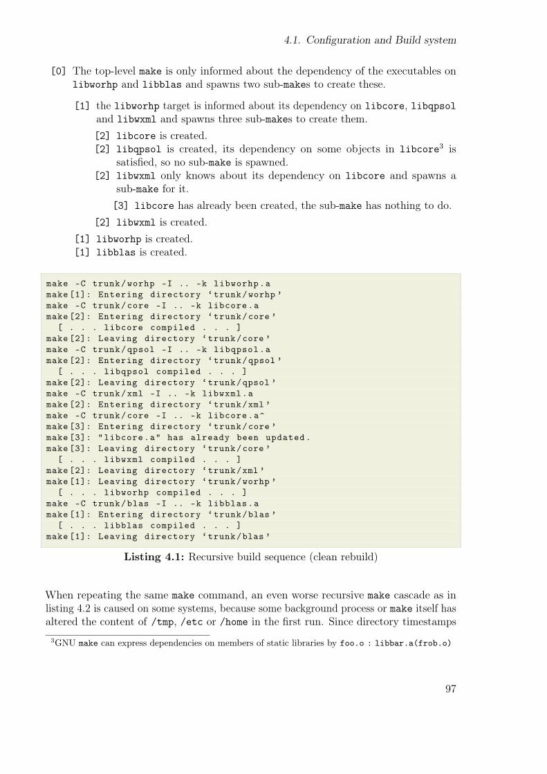
4.1. Configuration and Build system
[0] The top-level make is only informed about the dependency of the executables onlibworhp and libblas and spawns two sub-makes to create these.
[1] the libworhp target is informed about its dependency on libcore, libqpsoland libwxml and spawns three sub-makes to create them.
[2] libcore is created.[2] libqpsol is created, its dependency on some objects in libcore3 is
satisőed, so no sub-make is spawned.[2] libwxml only knows about its dependency on libcore and spawns a
sub-make for it.
[3] libcore has already been created, the sub-make has nothing to do.
[2] libwxml is created.
[1] libworhp is created.[1] libblas is created.
make -C trunk/worhp -I .. -k libworhp.a
make [1]: Entering directory ‘trunk/worhp ’
make -C trunk/core -I .. -k libcore.a
make [2]: Entering directory ‘trunk/core ’
[ . . . libcore compiled . . . ]
make [2]: Leaving directory ‘trunk/core ’
make -C trunk/qpsol -I .. -k libqpsol.a
make [2]: Entering directory ‘trunk/qpsol ’
[ . . . libqpsol compiled . . . ]
make [2]: Leaving directory ‘trunk/qpsol ’
make -C trunk/xml -I .. -k libwxml.a
make [2]: Entering directory ‘trunk/xml ’
make -C trunk/core -I .. -k libcore.a^
make [3]: Entering directory ‘trunk/core ’
make [3]: "libcore.a" has already been updated.
make [3]: Leaving directory ‘trunk/core ’
[ . . . libwxml compiled . . . ]
make [2]: Leaving directory ‘trunk/xml ’
make [1]: Leaving directory ‘trunk/worhp ’
[ . . . libworhp compiled . . . ]
make -C trunk/blas -I .. -k libblas.a
make [1]: Entering directory ‘trunk/blas ’
[ . . . libblas compiled . . . ]
make [1]: Leaving directory ‘trunk/blas ’
Listing 4.1: Recursive build sequence (clean rebuild)
When repeating the same make command, an even worse recursive make cascade as inlisting 4.2 is caused on some systems, because some background process or make itself hasaltered the content of /tmp, /etc or /home in the őrst run. Since directory timestamps
3GNU make can express dependencies on members of static libraries by foo.o : libbar.a(frob.o)
97

4. Solver Infrastructure
on Linux change when the directory content is altered, these now have newer timestampsthan the Worhp sub-libraries; presumably due to some of the many implicit rules ofGNU make, the sub-libraries are considered as outdated and make spawns sub-makes toupdate them. The sub-makes then correctly deduce that nothing has to be done, since nosource or object őle is actually newer than the respective static library, and thus do nottouch them, keeping their timestamp unmodiőed. This results in repeated spawning ofredundant sub-makes, e.g. 3 times for libcore (as dependency of libworhp, of libqpsoland libwxml).
make -C trunk/worhp -I .. -k libworhp.a
make [1]: Entering directory ‘trunk/worhp ’
make -C trunk/core -I .. -k libcore.a
make [2]: Entering directory ‘trunk/core ’
make [2]: "libcore.a" has already been updated.
make [2]: Leaving directory ‘trunk/core ’
make -C trunk/qpsol -I .. -k libqpsol.a
make [2]: Entering directory ‘trunk/qpsol ’
make [2]: "libqpsol.a" has already been updated.
make [2]: Leaving directory ‘trunk/qpsol ’
make -C trunk/xml -I .. -k libwxml.a
make [2]: Entering directory ‘trunk/xml ’
make -C trunk/core -I .. -k libcore.a
make [3]: Entering directory ‘trunk/core ’
make [3]: "libcore.a" has already been updated.
make [3]: Leaving directory ‘trunk/core ’
make [2]: Leaving directory ‘trunk/xml ’
make [1]: Leaving directory ‘trunk/worhp ’
make -C trunk/xml -I .. -k libwxml.a
make [1]: Entering directory ‘trunk/xml ’
make -C trunk/core -I .. -k libcore.a
make [2]: Entering directory ‘trunk/core ’
make [2]: "libcore.a" has already been updated.
make [2]: Leaving directory ‘trunk/core ’
make [1]: Leaving directory ‘trunk/xml ’
make -C trunk/qpsol -I .. -k libqpsol.a
make [1]: Entering directory ‘trunk/qpsol ’
make [1]: "libqpsol.a" has already been updated.
make [1]: Leaving directory ‘trunk/qpsol ’
make -C trunk/core -I .. -k libcore.a
make [1]: Entering directory ‘trunk/core ’
make [1]: "libcore.a" has already been updated.
make [1]: Leaving directory ‘trunk/core ’
make -C trunk/blas -I .. -k libblas.a
make [1]: Entering directory ‘trunk/blas ’
make [1]: Nothing to be done for "libblas.a".
make [1]: Leaving directory ‘trunk/blas ’
Listing 4.2: Recursive build cascade due to newer őle system timestamps
The initial recursive build system thus causes unnecessary overhead due to suboptimaluse of the dependency tracking features of make.
98
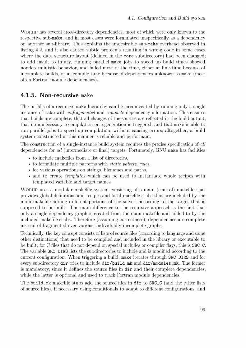
4.1. Configuration and Build system
Worhp has several cross-directory dependencies, most of which were only known to therespective sub-make, and in most cases were formulated unspeciőcally as a dependencyon another sub-library. This explains the undesirable sub-make overhead observed inlisting 4.2, and it also caused subtle problems resulting in wrong code in some caseswhere the data structure layout (deőned in the core subdirectory) had been changed;to add insult to injury, running parallel make jobs to speed up build times showednondeterministic behavior, and failed most of the time, either at link-time because ofincomplete builds, or at compile-time because of dependencies unknown to make (mostoften Fortran module dependencies).
4.1.5. Non-recursive make
The pitfalls of a recursive make hierarchy can be circumvented by running only a singleinstance of make with unfragmented and complete dependency information. This ensuresthat builds are complete, that all changes of the sources are reŕected in the build output,that no unnecessary recompilation or regeneration is triggered, and that make is able torun parallel jobs to speed up compilation, without causing errors; altogether, a buildsystem constructed in this manner is reliable and performant.
The construction of a single-instance build system requires the precise speciőcation of alldependencies for all (intermediate or őnal) targets. Fortunately, GNU make has facilities
• to include makeőles from a list of directories,• to formulate multiple patterns with static pattern rules,• for various operations on strings, őlenames and paths,• and to create templates which can be used to instantiate whole recipes with
templated variable and target names.
Worhp uses a modular makeőle system consisting of a main (central) makeőle thatprovides global deőnitions and recipes and local makeőle stubs that are included by themain makeőle adding diferent portions of the solver, according to the target that issupposed to be built. The main diference to the recursive approach is the fact thatonly a single dependency graph is created from the main makeőle and added to by theincluded makeőle stubs. Therefore (assuming correctness), dependencies are completeinstead of fragmented over various, individually incomplete graphs.
Technically, the key concept consists of lists of source őles (according to language and someother distinctions) that need to be compiled and included in the library or executable tobe built; for C őles that do not depend on special includes or compiler ŕags, this is SRC_C.The variable SRC_DIRS lists the subdirectories to include and is modiőed according to thecurrent conőguration. When triggering a build, make iterates through SRC_DIRS and forevery subdirectory dir tries to include dir/build.mk and dir/modules.mk. The formeris mandatory, since it deőnes the source őles in dir and their complete dependencies,while the latter is optional and used to track Fortran module dependencies.
The build.mk makeőle stubs add the source őles in dir to SRC_C (and the other listsof source őles), if necessary using conditionals to adapt to diferent conőgurations, and
99
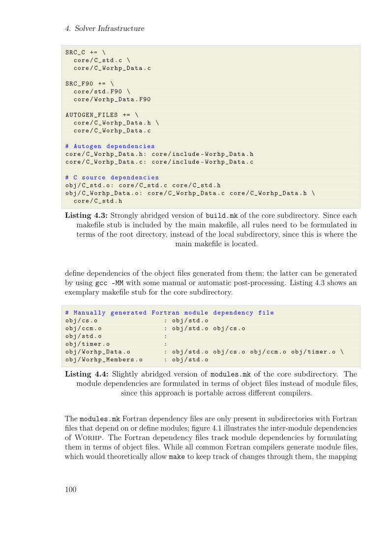
4. Solver Infrastructure
SRC_C += \
core/C_std.c \
core/C_Worhp_Data.c
SRC_F90 += \
core/std.F90 \
core/Worhp_Data.F90
AUTOGEN_FILES += \
core/C_Worhp_Data.h \
core/C_Worhp_Data.c
# Autogen dependencies
core/C_Worhp_Data.h: core/include -Worhp_Data.h
core/C_Worhp_Data.c: core/include -Worhp_Data.c
# C source dependencies
obj/C_std.o: core/C_std.c core/C_std.h
obj/C_Worhp_Data.o: core/C_Worhp_Data.c core/C_Worhp_Data.h \
core/C_std.h
Listing 4.3: Strongly abridged version of build.mk of the core subdirectory. Since eachmakeőle stub is included by the main makeőle, all rules need to be formulated interms of the root directory, instead of the local subdirectory, since this is where the
main makeőle is located.
deőne dependencies of the object őles generated from them; the latter can be generatedby using gcc -MM with some manual or automatic post-processing. Listing 4.3 shows anexemplary makeőle stub for the core subdirectory.
# Manually generated Fortran module dependency file
obj/cs.o : obj/std.o
obj/ccm.o : obj/std.o obj/cs.o
obj/std.o :
obj/timer.o :
obj/Worhp_Data.o : obj/std.o obj/cs.o obj/ccm.o obj/timer.o \
obj/Worhp_Members.o : obj/std.o
Listing 4.4: Slightly abridged version of modules.mk of the core subdirectory. Themodule dependencies are formulated in terms of object őles instead of module őles,
since this approach is portable across diferent compilers.
The modules.mk Fortran dependency őles are only present in subdirectories with Fortranőles that depend on or deőne modules; őgure 4.1 illustrates the inter-module dependenciesof Worhp. The Fortran dependency őles track module dependencies by formulatingthem in terms of object őles. While all common Fortran compilers generate module őles,which would theoretically allow make to keep track of changes through them, the mapping
100
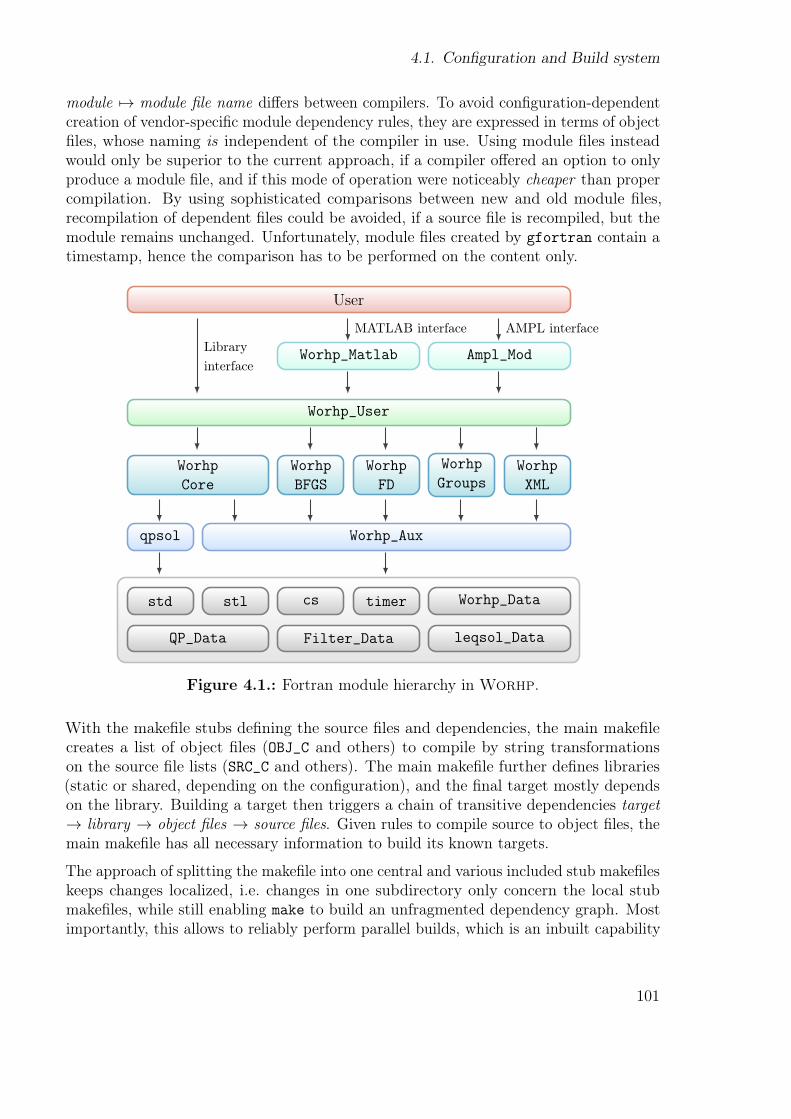
4.1. Configuration and Build system
module →→ module file name difers between compilers. To avoid conőguration-dependentcreation of vendor-speciőc module dependency rules, they are expressed in terms of objectőles, whose naming is independent of the compiler in use. Using module őles insteadwould only be superior to the current approach, if a compiler ofered an option to onlyproduce a module őle, and if this mode of operation were noticeably cheaper than propercompilation. By using sophisticated comparisons between new and old module őles,recompilation of dependent őles could be avoided, if a source őle is recompiled, but themodule remains unchanged. Unfortunately, module őles created by gfortran contain atimestamp, hence the comparison has to be performed on the content only.
User
Library
interface
MATLAB interface AMPL interface
Worhp_Matlab Ampl_Mod
Worhp_User
Worhp
Core
Worhp
BFGS
Worhp
FD
Worhp
GroupsWorhp
XML
qpsol Worhp_Aux
std stl cs timer Worhp_Data
QP_Data Filter_Data leqsol_Data
Figure 4.1.: Fortran module hierarchy in Worhp.
With the makeőle stubs deőning the source őles and dependencies, the main makeőlecreates a list of object őles (OBJ_C and others) to compile by string transformationson the source őle lists (SRC_C and others). The main makeőle further deőnes libraries(static or shared, depending on the conőguration), and the őnal target mostly dependson the library. Building a target then triggers a chain of transitive dependencies target→ library → object files → source files. Given rules to compile source to object őles, themain makeőle has all necessary information to build its known targets.
The approach of splitting the makeőle into one central and various included stub makeőleskeeps changes localized, i.e. changes in one subdirectory only concern the local stubmakeőles, while still enabling make to build an unfragmented dependency graph. Mostimportantly, this allows to reliably perform parallel builds, which is an inbuilt capability
101
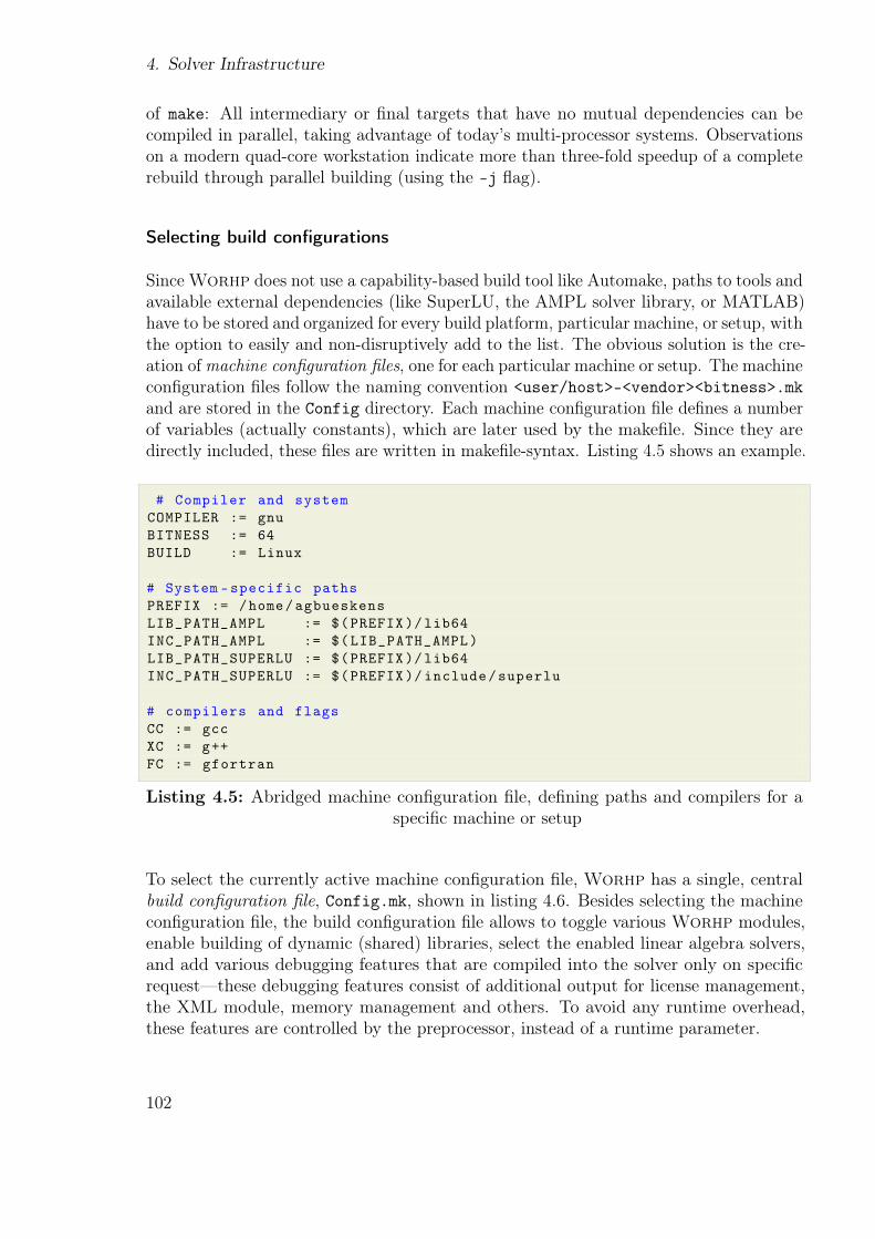
4. Solver Infrastructure
of make: All intermediary or őnal targets that have no mutual dependencies can becompiled in parallel, taking advantage of today’s multi-processor systems. Observationson a modern quad-core workstation indicate more than three-fold speedup of a completerebuild through parallel building (using the -j ŕag).
Selecting build configurations
Since Worhp does not use a capability-based build tool like Automake, paths to tools andavailable external dependencies (like SuperLU, the AMPL solver library, or MATLAB)have to be stored and organized for every build platform, particular machine, or setup, withthe option to easily and non-disruptively add to the list. The obvious solution is the cre-ation of machine configuration files, one for each particular machine or setup. The machineconőguration őles follow the naming convention <user/host>-<vendor><bitness>.mk
and are stored in the Config directory. Each machine conőguration őle deőnes a numberof variables (actually constants), which are later used by the makeőle. Since they aredirectly included, these őles are written in makeőle-syntax. Listing 4.5 shows an example.
# Compiler and system
COMPILER := gnu
BITNESS := 64
BUILD := Linux
# System -specific paths
PREFIX := /home/agbueskens
LIB_PATH_AMPL := $(PREFIX )/lib64
INC_PATH_AMPL := $(LIB_PATH_AMPL)
LIB_PATH_SUPERLU := $(PREFIX )/lib64
INC_PATH_SUPERLU := $(PREFIX )/ include/superlu
# compilers and flags
CC := gcc
XC := g++
FC := gfortran
Listing 4.5: Abridged machine conőguration őle, deőning paths and compilers for aspeciőc machine or setup
To select the currently active machine conőguration őle, Worhp has a single, centralbuild configuration file, Config.mk, shown in listing 4.6. Besides selecting the machineconőguration őle, the build conőguration őle allows to toggle various Worhp modules,enable building of dynamic (shared) libraries, select the enabled linear algebra solvers,and add various debugging features that are compiled into the solver only on speciőcrequestÐthese debugging features consist of additional output for license management,the XML module, memory management and others. To avoid any runtime overhead,these features are controlled by the preprocessor, instead of a runtime parameter.
102
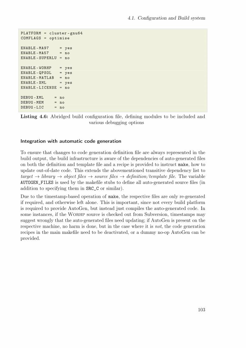
4.1. Configuration and Build system
PLATFORM = cluster -gnu64
COMFLAGS = optimise
ENABLE -MA97 = yes
ENABLE -MA57 = no
ENABLE -SUPERLU = no
ENABLE -WORHP = yes
ENABLE -QPSOL = yes
ENABLE -MATLAB = no
ENABLE -XML = yes
ENABLE -LICENSE = no
DEBUG -XML = no
DEBUG -MEM = no
DEBUG -LIC = no
Listing 4.6: Abridged build conőguration őle, deőning modules to be included andvarious debugging options
Integration with automatic code generation
To ensure that changes to code generation deőnition őle are always represented in thebuild output, the build infrastructure is aware of the dependencies of auto-generated őleson both the deőnition and template őle and a recipe is provided to instruct make, how toupdate out-of-date code. This extends the abovementioned transitive dependency list totarget → library → object files → source files → definition/template file. The variableAUTOGEN_FILES is used by the makeőle stubs to deőne all auto-generated source őles (inaddition to specifying them in SRC_C or similar).
Due to the timestamp-based operation of make, the respective őles are only re-generatedif required, and otherwise left alone. This is important, since not every build platformis required to provide AutoGen, but instead just compiles the auto-generated code. Insome instances, if the Worhp source is checked out from Subversion, timestamps maysuggest wrongly that the auto-generated őles need updating; if AutoGen is present on therespective machine, no harm is done, but in the case where it is not, the code generationrecipes in the main makeőle need to be deactivated, or a dummy no-op AutoGen can beprovided.
103
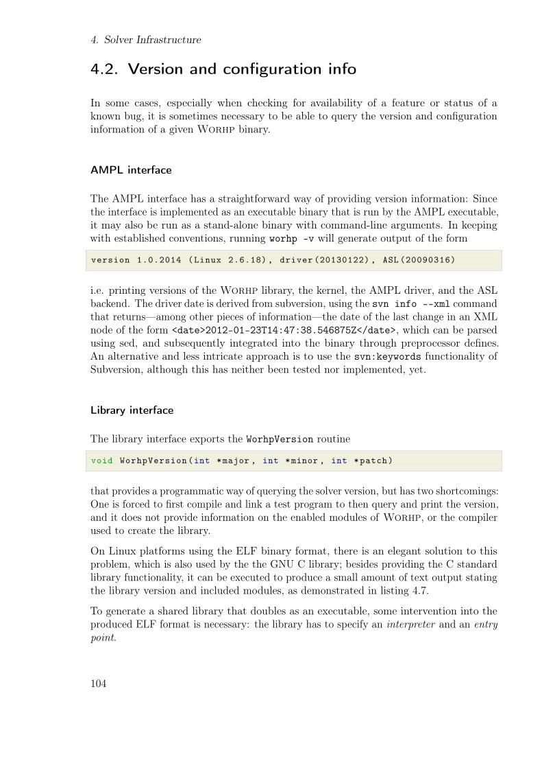
4. Solver Infrastructure
4.2. Version and configuration info
In some cases, especially when checking for availability of a feature or status of aknown bug, it is sometimes necessary to be able to query the version and conőgurationinformation of a given Worhp binary.
AMPL interface
The AMPL interface has a straightforward way of providing version information: Sincethe interface is implemented as an executable binary that is run by the AMPL executable,it may also be run as a stand-alone binary with command-line arguments. In keepingwith established conventions, running worhp -v will generate output of the form
version 1.0.2014 (Linux 2.6.18) , driver (20130122) , ASL (20090316)
i.e. printing versions of the Worhp library, the kernel, the AMPL driver, and the ASLbackend. The driver date is derived from subversion, using the svn info --xml commandthat returnsÐamong other pieces of informationÐthe date of the last change in an XMLnode of the form <date>2012-01-23T14:47:38.546875Z</date>, which can be parsedusing sed, and subsequently integrated into the binary through preprocessor deőnes.An alternative and less intricate approach is to use the svn:keywords functionality ofSubversion, although this has neither been tested nor implemented, yet.
Library interface
The library interface exports the WorhpVersion routine
void WorhpVersion(int *major , int *minor , int *patch)
that provides a programmatic way of querying the solver version, but has two shortcomings:One is forced to őrst compile and link a test program to then query and print the version,and it does not provide information on the enabled modules of Worhp, or the compilerused to create the library.
On Linux platforms using the ELF binary format, there is an elegant solution to thisproblem, which is also used by the the GNU C library; besides providing the C standardlibrary functionality, it can be executed to produce a small amount of text output statingthe library version and included modules, as demonstrated in listing 4.7.
To generate a shared library that doubles as an executable, some intervention into theproduced ELF format is necessary: the library has to specify an interpreter and an entrypoint.
104
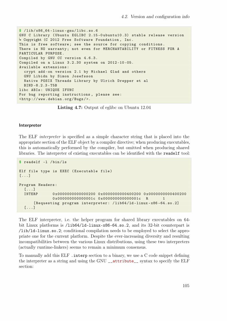
4.2. Version and configuration info
$ /lib/x86_64 -linux -gnu/libc.so.6
GNU C Library (Ubuntu EGLIBC 2.15 -0 ubuntu10 .3) stable release version
Copyright (C 2012 Free Software Foundation , Inc.
This is free software; see the source for copying conditions.
There is NO warranty; not even for MERCHANTABILITY or FITNESS FOR A
PARTICULAR PURPOSE.
Compiled by GNU CC version 4.6.3.
Compiled on a Linux 3.2.30 system on 2012 -10 -05.
Available extensions:
crypt add -on version 2.1 by Michael Glad and others
GNU Libidn by Simon Josefsson
Native POSIX Threads Library by Ulrich Drepper et al
BIND -8.2.3 - T5B
libc ABIs: UNIQUE IFUNC
For bug reporting instructions , please see:
<http ://www.debian.org/Bugs/>.
Listing 4.7: Output of eglibc on Ubuntu 12.04
Interpreter
The ELF interpreter is speciőed as a simple character string that is placed into theappropriate section of the ELF object by a compiler directive; when producing executables,this is automatically performed by the compiler, but omitted when producing sharedlibraries. The interpreter of existing executables can be identiőed with the readelf tool:
$ readelf -l /bin/ls
Elf file type is EXEC (Executable file)
[...]
Program Headers:
[...]
INTERP 0x0000000000000200 0x0000000000400200 0x0000000000400200
0x000000000000001c 0x000000000000001c R 1
[Requesting program interpreter: /lib64/ld -linux -x86 -64.so.2]
[...]
The ELF interpreter, i.e. the helper program for shared library executables on 64-bit Linux platforms is /lib64/ld-linux-x86-64.so.2, and its 32-bit counterpart is/lib/ld-linux.so.2; conditional compilation needs to be employed to select the appro-priate one for the current platform. Despite the ever-increasing diversity and resultingincompatibilities between the various Linux distributions, using these two interpreters(actually runtime-linkers) seems to remain a minimum consensus.
To manually add this ELF .interp section to a binary, we use a C code snippet deőningthe interpreter as a string and using the GNU __attribute__ syntax to specify the ELFsection:
105
4. Solver Infrastructure
const char elf_interpreter [] __attribute__ (( section(".interp"))) =
"/lib/ld -linux.so.2";
Entry point
To specify the entry point, which again is automatically performed by the linker whenproducing an executable, the -e option to the linker speciőes the function to be used asentry point (usually main for executables). To embed this into the GCC command-linethat links the shared library, the -Wl syntax for passing options to the linker has to beused, resulting in
-Wl,-e,entry_point
to deőne entry_point as the entry point function; commas need to be used to prevent theusual tokenization by the compiler driver of the linker options at whitespace, otherwise-e entry_point would be passed to the compiler instead of the linker (resulting incomplaints, because GCC does not understand this option).
Combining both these techniques is used to have libworhp.so print informative outputshown in listing 4.8.
$ libworhp.so
WORHP shared library for Linux , version 1.0.2014
Copyright (C) 2013 SFZ Optimierung , Steuerung und Regelung.
Distribution of WORHP is subject to terms and conditions.
The authors disclaim all warranties , including without limitation ,
merchantability or fitness for a particular purpose.
Available modules:
MA97 solver support
SuperLU solver support
XML module
Compiled with:
gcc (Ubuntu/Linaro 4.6.3 -1 ubuntu5) 4.6.3
GNU Fortran (Ubuntu/Linaro 4.6.3 -1 ubuntu5) 4.6.3
Listing 4.8: Sample output of shared libworhp on Linux platforms
106

4.3. Testing Approach
4.3. Testing Approach
Debugging is twice as hard as writing the code in the firstplace. Therefore, if you write code as cleverly as possible, youare, by definition, not smart enough to debug it.
(Brian Kernighan)
Although the development process of Worhp has never been subject to strict formaliza-tion, it does share some characteristics with the test-driven development paradigm.
Test-driven development is characterized by creating tests for desired functionality beforecreating the software to be tested. This approach guarantees good test coverage andadditionally provides a simple metric for changes to the software. Regression Testing isa canonic addition to this development method, its main diference being that its testsprovoke known (and usually corrected) defects in the software, instead of testing desiredfunctionality. In the combined approach, the test suite is őrst populated with tests forfunctionality that is to be developed, and over the lifespan of the software, tests foridentiőed bugs are added to prevent regressions. The GNU Compiler Collection embracesthis approach and has accumulated over 40,000 such tests over the course of its 25-yearlifetime.
Since Worhp is built to solve NLP, its test suite will naturally consist of optimizationproblems, accompanied by the technical infrastructure needed to run all tests and verifytheir outcome. To make a meaningful statement about Worhp’s capabilities, the test setneeds to be as diverse as possible. The default test suites are a 920-problem set writtenin AMPL, consisting of a subset of CUTEr plus the Schittkowski problems from [63], andthe 68-problem COPS test set. The genuine CUTEr collection is provided as 11474 őlesin SIF format. Since Worhp does not (yet) have a SIF interface, the AMPL alternativeis used for testing. Although neither is a true subset of the other, we shall refer to theset as ł(AMPL-)CUTErž.
Both CUTEr and COPS are recognized as standard test sets for benchmarking andcomparing NLP solvers by the mathematical optimization community, with COPS evenbeing speciőcally designed as solver comparison tool, and CUTEr containing the 124Hock/Schittkowski NLP test problems[32] many of which were speciőcally written toexploit known weaknesses in SQP solvers.
Testing in our sense means to feed all or a subset of the optimization problems ofthe abovementioned test sets to the solver. Test results are derived from some canonicquantities for NLP, among which are the objective function value, the constraint violation,an optimality measure, iteration and function evaluation counts and user time, and thesolver status (solved to optimal or acceptable level, or some error condition). Test runs,such as a typical before/after check when a modiőcation is introduced, can then becompared according to an arbitrary performance measure.
4as of 2012-06 – the collection is updated irregularly, see ftp://ftp.numerical.rl.ac.uk/pub/cuter/mastsif.updates
107
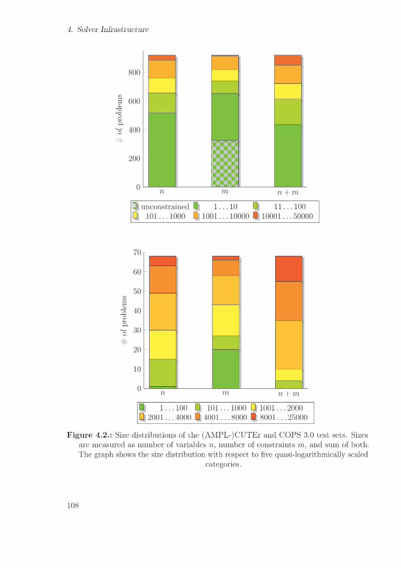
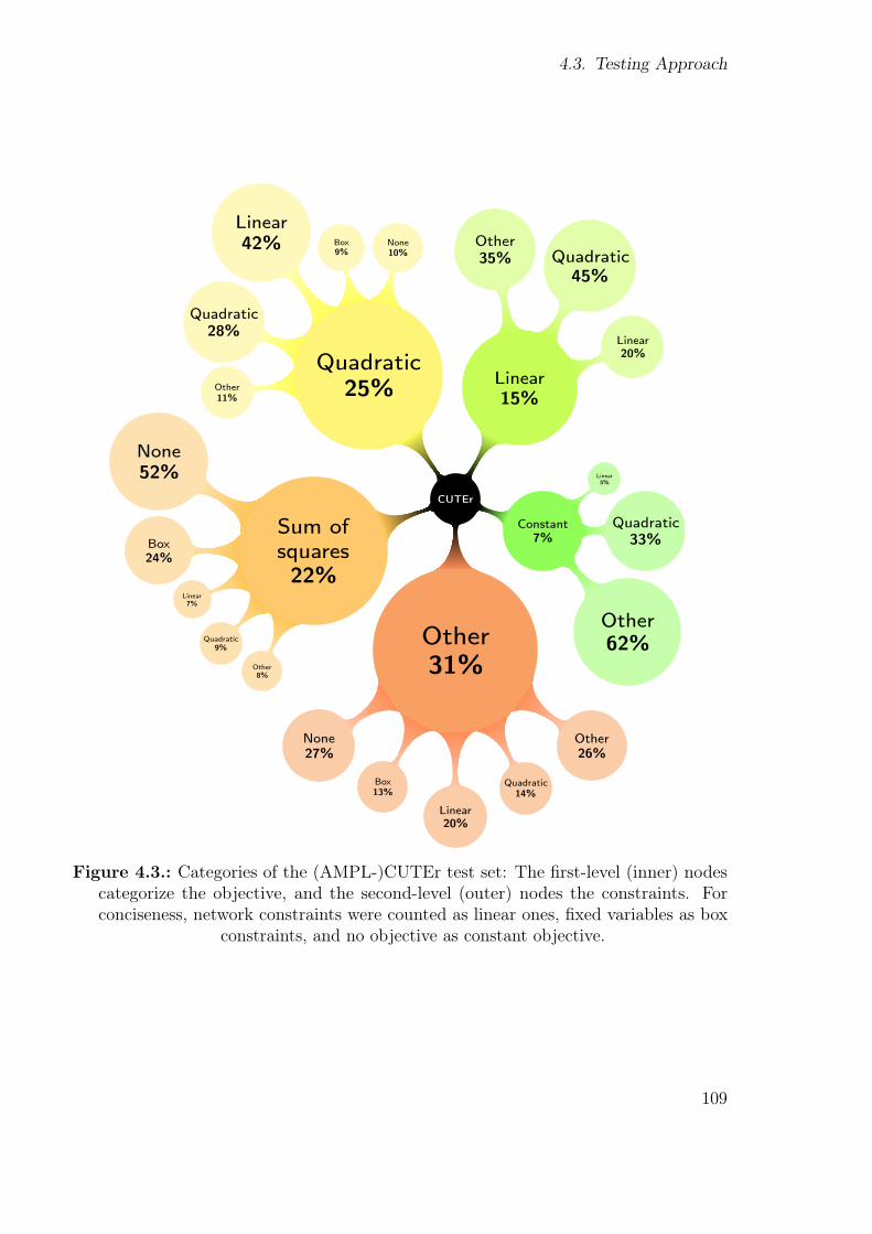
4.3. Testing Approach
CUTEr
Constant
7%
Other
62%
Quadratic
33%
Linear
5%
Linear
15%
Linear
20%
Quadratic
45%
Other
35%
Quadratic
25%
None
10%
Box
9%
Linear
42%
Quadratic
28%
Other
11%
Sum of
squares
22%
None
52%
Box
24%
Linear
7%
Quadratic
9%
Other
8%
Other
31%
None
27%
Box
13%
Linear
20%
Quadratic
14%
Other
26%
Figure 4.3.: Categories of the (AMPL-)CUTEr test set: The őrst-level (inner) nodescategorize the objective, and the second-level (outer) nodes the constraints. Forconciseness, network constraints were counted as linear ones, őxed variables as box
constraints, and no objective as constant objective.
109
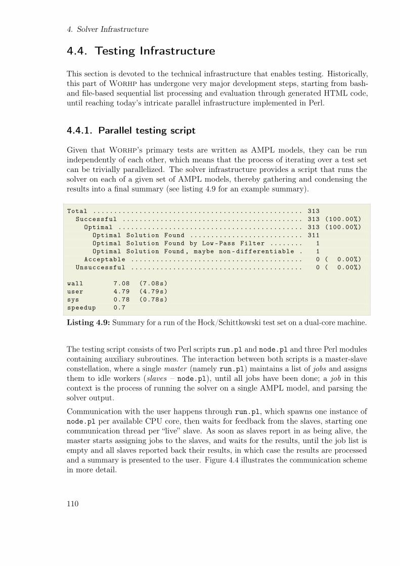
4. Solver Infrastructure
4.4. Testing Infrastructure
This section is devoted to the technical infrastructure that enables testing. Historically,this part of Worhp has undergone very major development steps, starting from bash-and őle-based sequential list processing and evaluation through generated HTML code,until reaching today’s intricate parallel infrastructure implemented in Perl.
4.4.1. Parallel testing script
Given that Worhp’s primary tests are written as AMPL models, they can be runindependently of each other, which means that the process of iterating over a test setcan be trivially parallelized. The solver infrastructure provides a script that runs thesolver on each of a given set of AMPL models, thereby gathering and condensing theresults into a őnal summary (see listing 4.9 for an example summary).
Total .................................................. 313
Successful ........................................... 313 (100.00%)
Optimal ............................................ 313 (100.00%)
Optimal Solution Found ........................... 311
Optimal Solution Found by Low -Pass Filter ........ 1
Optimal Solution Found , maybe non -differentiable . 1
Acceptable ......................................... 0 ( 0.00%)
Unsuccessful ......................................... 0 ( 0.00%)
wall 7.08 (7.08s)
user 4.79 (4.79s)
sys 0.78 (0.78s)
speedup 0.7
Listing 4.9: Summary for a run of the Hock/Schittkowski test set on a dual-core machine.
The testing script consists of two Perl scripts run.pl and node.pl and three Perl modulescontaining auxiliary subroutines. The interaction between both scripts is a master-slaveconstellation, where a single master (namely run.pl) maintains a list of jobs and assignsthem to idle workers (slaves ś node.pl), until all jobs have been done; a job in thiscontext is the process of running the solver on a single AMPL model, and parsing thesolver output.
Communication with the user happens through run.pl, which spawns one instance ofnode.pl per available CPU core, then waits for feedback from the slaves, starting onecommunication thread per łlivež slave. As soon as slaves report in as being alive, themaster starts assigning jobs to the slaves, and waits for the results, until the job list isempty and all slaves reported back their results, in which case the results are processedand a summary is presented to the user. Figure 4.4 illustrates the communication schemein more detail.
110
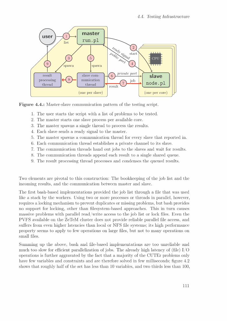
4. Solver Infrastructure
and even fewer constraints. It is therefore necessary to have sub-microsecond access tothe job list, hence a performant implementation has to hold it in memory. This requiresexplicit communication between master and slave, because the slaves cannot retrieve jobsfrom a globally visible őle anymore. The latency of this communication link needs to belower (preferably by at least one order of magnitude) than the time spent on executingthe job.
Since bash does not provide adequate tools for either, the current implementation usesPerl, with the master-slave communication implemented through Ethernet connectionsand the job and result lists implemented on top of a thread-safe deque.
The deque is a Thread::Queue, which is fast and thread-safe. The Ethernet connection onmulti-core machines (i.e. an SMP setup) will be routed through the loopback device, whichincurs very low latencies, and in clusters or MPP setups typically has sub-microsecondlatency. The ZeTeM cluster, for example, is equipped with high-performance Inőnibandand Gigabit Ethernet, which have proven to achieve suiciently low latencies for runninghundreds of jobs in parallel without performance problemsÐping latencies usually lie inthe 50− 100µs range and thus do not dominate the total time, even for small problems.
Higher network latencies are commonly found in distributed (cloud) computing, wherethe individual nodes are not connected through a local network but over regular internetconnections, which results in typical latencies in the 20− 40ms range, i.e. between twoand three orders of magnitude greater than in local clusters. Grouping individually smalltasks into bigger jobs that again take (noticeably) more time to őnish is an option tokeep the network latency from dominating the total time and increase the CPU workload.
The advantage of using TCP connections is that the test infrastructure can be run withoutmodiőcation on very diferent machine types and network topologies, such as a multi-coredesktop machine, a dedicated compute cluster, or a distributed computing grid. Onlythe method of starting the slaves has to be tailored to the present infrastructure: On amulti-core machine, the slaves are started as child processes, while on the ZeTeM cluster,the PBS scheduler distributes and starts the slaves.
Termination
With all jobs distributed, the next important question concerns the termination of theparallel run script: How does the script notice that all jobs have been completed? Theleast-technical approach is to compare the total number of jobs against the number ofreceived results; once the latter reaches the former, all jobs have been completed. Thisapproach is simple and eicient, but vulnerable to faults: A single job that fails toproduce results will cause the whole run to fail, since the őnal processing and condensingof all results can only be triggered as soon as all results are available. It is thereforenecessary to őnd a more fault-tolerant solution. In case of failing jobs, this will result inincomplete results, but ŕawed results are preferable over no results at all.
The chosen approach monitors the number of slave communication threads instead of thenumber of results : After starting the slaves and the result processing thread (2 and 3 in
112
4.4. Testing Infrastructure
őgure 4.4), the master starts a thread that is waiting for incoming TCP connections onthe public port (4), and for every such connection spawns a communication thread (5)that uses a dedicated private port to connect to its associated slave (6). If the slave diesor if it reported its results and the communication thread has no more jobs to submit, itterminates itself. Monitoring the number of live slave communication threads is thereforea feasible termination criterion that is robust against faults: If all slave communicationthreads have terminated, all jobs have been sent to the slaves and either returned resultsor were lost. To sum up, this approach is more robust than counting results, but still hasfollowing ŕaws:
• It is more complex than the result-counting approach; in particular, the main threadőrst has to wait for at least one slave communication thread to start, before waitingfor all threads to finish againÐwithout this barrier, there is a race condition in whichthe main thread terminates right away, if no slave communication thread has beenspawned, yet. To implement such a barrier, Perl’s cond_wait and cond_signal
are used.• The master thread that listens for incoming TCP connections on the public port
will never terminate; as soon as all possible slaves have been started, no additionalconnections will come in, leaving the master thread blocked. Since the Perl threadimplementation does not ofer mechanisms to terminate a thread from outside, thethread cannot terminate or be terminated gracefully. Fortunately, this is of littlepractical relevance, because Perl terminates all threads if the spawning programends, but this provokes warning messages about łrunning and detached threadsžthat may irritate inexperienced users.
• Slaves may suddenly die, either due to errors in the called program (in our case theWorhp binary) or due to external inŕuences, such as hardware errors, hung-upkernels or out-of-memory situations. This approach was devised to handle dyingslaves gracefully, but should nevertheless try and obtain results for every job. If theslave communication thread notices that its slave has died, it therefore re-submitsthe last job to the job queue to have another slave process it. This is reasonable ifthe slave died due to some external inŕuence, but will result in a cascade of dyingslaves, if the job is responsible.
4.4.2. Solver output processing
Condensing the results is concerned with parsing the solver output, performing operations(string comparisons, count, sum, mean, . . . ) on various numeric quantities or status stringsand formatting the results for outputÐstep 9 in őgure 4.4. The parsing is performed byredirecting the solver output through a solver-speciőc parser (since the output formatsof diferent NLP solvers difer widely), which performs line-by-line pattern matchingto extract counts of function evaluation, major and minor iterations, as well as timinginformation, achieved results (objective, feasibility and optimality) and the terminationstatus. Listing 4.10 shows an example of the condensed output on the master node.
113
4. Solver Infrastructure
The solver output parsers are implemented as stateless functions invoked for every lineof solver output, which complicates matters, if some piece of information has to bederived from multiple lines ś most prominently the constraint count, which is oftendisplayed over various lines, diferentiating between equality and inequality constraints,or upper/lower/both bounds for box constraints. A workaround is to make the outputparsing routines stateful by using global variables, such that summation over variouslines is possible.
The solver output parsers (one for each NLP solver) have proven to be quite fragile, sincesubtle changes in the output format of the solver may cause portions of the parser to fail,which in turn leads to undeőned values in the sweep script.
Timing the solvers is performed by starting them through the external time command,providing wall time, user time and sys time. This approach was chosen, because someNLP solvers do not provide timing routines, whereas the internal timing results of othersdifer signiőcantly from external timing. A uniform external timing tool is therefore thefairest comparison between diferent solvers.
Performance Considerations
Running the (AMPL-)CUTEr test set produces 111,110 (sic) lines of output5 with anoverall 8,360,502 bytes, amounting to an average of 120 lines per problem, and roughly 250lines or 18,200 bytes per second on an Intel i7-2600 system with 8 (virtual) cores. Scalingup to the 320 cores of the ZeTeM cluster, this could theoretically produce 10,000 linesper second with 728 KB/s (≈ 5.6 Mbps) of solver output per second to be sent throughthe network and parsed by the master node. While a 100 Mbit Ethernet connection caneasily handle 5 Mbps of data, it is unclear whether Perl can parse this continuous datastream in real-time. In extreme cases, this could lead to overŕowing bufers and dataloss and consequently in incorrect results.
With the sweep functionality being embedded into the parallel run script, the majorparsing efort is therefore delegated to the slaves to keep the CPU load of the masternode and the amount of network traic as low as possible. The master node only receivesthe parsed results, which are sent over the network in the form of őxed-layout strings like
DONE tag =000000: name=hs005:n=2:m=4:nf=11:ng=0: iter =10:
obj = -1.9132229545E+00: con =0.0000000000E+00: kkt =7.7493642313E-08:
status=Optimal Solution Found:tuser =0.00: tsys =0.00
The master caches the received result strings in a Thread::Queue deque, which feeds intothe result processing thread (step 8 in őgure 4.4). To process, each string is tokenized, andPerl’s inbuilt regular expression matching is applied to extract the values. Informationon queue length is indicated below the test results; low values indicate that the resultprocessing thread is able to keep up with the incoming stream of results, while highvalues indicate overload.
5trunk, revision 1949, default settings
114
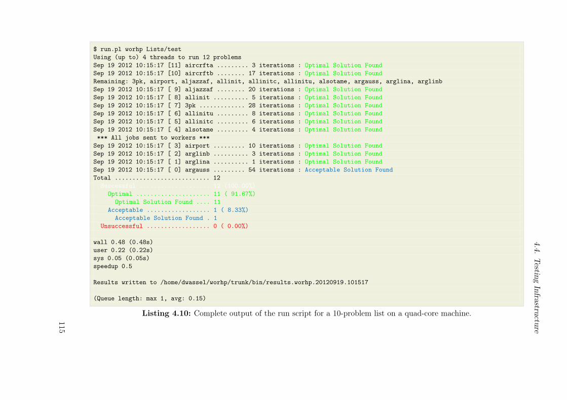
4.4
.Testin
gIn
frastru
cture
$ run.pl worhp Lists/test
Using (up to) 4 threads to run 12 problems
Sep 19 2012 10:15:17 [11] aircrfta ......... 3 iterations : Optimal Solution Found
Sep 19 2012 10:15:17 [10] aircrftb ........ 17 iterations : Optimal Solution Found
Remaining: 3pk, airport, aljazzaf, allinit, allinitc, allinitu, alsotame, argauss, arglina, arglinb
Sep 19 2012 10:15:17 [ 9] aljazzaf ........ 20 iterations : Optimal Solution Found
Sep 19 2012 10:15:17 [ 8] allinit .......... 5 iterations : Optimal Solution Found
Sep 19 2012 10:15:17 [ 7] 3pk ............. 28 iterations : Optimal Solution Found
Sep 19 2012 10:15:17 [ 6] allinitu ......... 8 iterations : Optimal Solution Found
Sep 19 2012 10:15:17 [ 5] allinitc ......... 6 iterations : Optimal Solution Found
Sep 19 2012 10:15:17 [ 4] alsotame ......... 4 iterations : Optimal Solution Found
*** All jobs sent to workers ***
Sep 19 2012 10:15:17 [ 3] airport ......... 10 iterations : Optimal Solution Found
Sep 19 2012 10:15:17 [ 2] arglinb .......... 3 iterations : Optimal Solution Found
Sep 19 2012 10:15:17 [ 1] arglina .......... 1 iterations : Optimal Solution Found
Sep 19 2012 10:15:17 [ 0] argauss ......... 54 iterations : Acceptable Solution Found
Total ........................... 12
Successful .................... 12 (100.00%)
Optimal ..................... 11 ( 91.67%)
Optimal Solution Found .... 11
Acceptable .................. 1 ( 8.33%)
Acceptable Solution Found . 1
Unsuccessful .................. 0 ( 0.00%)
wall 0.48 (0.48s)
user 0.22 (0.22s)
sys 0.05 (0.05s)
speedup 0.5
Results written to /home/dwassel/worhp/trunk/bin/results.worhp.20120919.101517
(Queue length: max 1, avg: 0.15)
Listing 4.10: Complete output of the run script for a 10-problem list on a quad-core machine.
115

4. Solver Infrastructure
4.5. Parameter Tuning
Sed quis emendabit ipso emendator?(But who will optimize the optimizer?)
(with apologies to Decimus Iunius Iuvenalis)
Being a complex piece of mathematical software, Worhp can be inŕuenced by morethan 100 runtime parameters. While the efects of some of them are obvious, for instanceMaxIter, Timeout or TolFeas (which are probably the most-used parameters and easilyunderstood by users), the inŕuence of many other parameters is much more diicult toassess, either because it is subtle and its details are intricate and require deep knowledge ofWorhp’s algorithmic or theoretical background, or because it changes major algorithmicdetails and thus potentially leads to completely diferent sequences of iterates. Whenregarding groups of parameters, instead of single parameters in isolation, the complexityof assessing parameter changes is complicated further (and probably growing exponentiallywith the size of the group).
4.5.1. Why tune solver parameters?
If the proper choice of parameters is diicult and mostly unintuitive, it is natural to askwhy users should struggle with it; since Worhp (and every other suiciently sophisticatedsoftware) is generic, its default parameters try and reŕect a minimum consensus for allpossible NLP, which is a huge and very diverse problem classÐwhen viewed pessimistically,this will necessarily be a setting that works badly for everyone, the software analogueto łone size őts allž. Thus, though not strictly necessary, tuning is often emphaticallyadvised when one intends to seriously solve optimization problems.
łTuningž may have very diferent meanings to diferent users and applications:
• In the prototype phase, parameter tuning may be necessary to achieve convergenceat all, since the model still has rough edges.
• If the underlying model is complex and somehow łhardž to solve, or if the achievableprecision is limited, careful tuning is often necessary to obtain satisfactory results.
• If the optimization result is subject to high precision requirements, parametertuning can ensure that these requirements are met.
• If a class of models has to be minimized frequently, the aim of parameter tuningwill be to speed up the optimization process.
Tuning is worthwhile, because the possible returns can be signiőcant, but it requiresa) deep mathematical, numerical and algorithmic insight into both the solver and theapplication, or b) great amounts of raw computing power to exhaustively sweep theparameter space on a set of representative examples.
Since approach a) is essentially limited to experienced NLP developers who are also deeplyknowledgeable about the potential application, approach b) is, though inelegant, a much
116
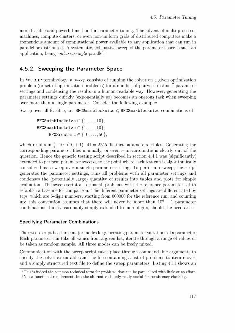
4.5. Parameter Tuning
more feasible and powerful method for parameter tuning. The advent of multi-processormachines, compute clusters, or even non-uniform grids of distributed computers make atremendous amount of computational power available to any application that can run inparallel or distributed. A systematic, exhaustive sweep of the parameter space is such anapplication, being embarrassingly parallel6.
4.5.2. Sweeping the Parameter Space
In Worhp terminology, a sweep consists of running the solver on a given optimizationproblem (or set of optimization problems) for a number of pairwise distinct7 parametersettings and condensing the results in a human-readable way. However, generating theparameter settings quickly (exponentially so) becomes an onerous task when sweepingover more than a single parameter. Consider the following example:
Sweep over all feasible, i.e. BFGSminblocksize 6 BFGSmaxblocksize combinations of
BFGSminblocksize ∈ {1, . . . , 10},BFGSmaxblocksize ∈ {1, . . . , 10},
BFGSrestart ∈ {10, . . . , 50},
which results in 12· 10 · (10 + 1) · 41 = 2255 distinct parameters triples. Generating the
corresponding parameter őles manually, or even semi-automatic is clearly out of thequestion. Hence the generic testing script described in section 4.4.1 was (signiőcantly)extended to perform parameter sweeps, to the point where each test run is algorithmicallyconsidered as a sweep over a single parameter setting. To perform a sweep, the scriptgenerates the parameter settings, runs all problems with all parameter settings andcondenses the (potentially large) quantity of results into tables and plots for simpleevaluation. The sweep script also runs all problems with the reference parameter set toestablish a baseline for comparison. The diferent parameter settings are diferentiated bytags, which are 6-digit numbers, starting from 000000 for the reference run, and countingup; this convention assumes that there will never be more than 106 − 1 parametercombinations, but is reasonably simply extended to more digits, should the need arise.
Specifying Parameter Combinations
The sweep script has three major modes for generating parameter variations of a parameter:Each parameter can take all values from a given list, iterate through a range of values orbe taken as random sample. All three modes can be freely mixed.
Communication with the sweep script takes place through command-line arguments tospecify the solver executable and the őle containing a list of problems to iterate over,and a simply structured text őle to deőne the sweep parameters. Listing 4.11 shows an
6This is indeed the common technical term for problems that can be parallelized with little or no effort.7Not a functional requirement, but the alternative is only really useful for consistency checking.
117
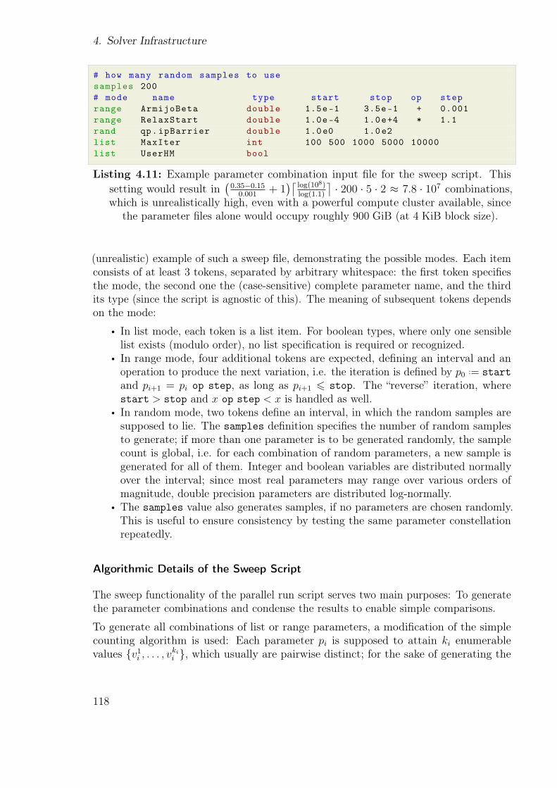
4. Solver Infrastructure
# how many random samples to use
samples 200
# mode name type start stop op step
range ArmijoBeta double 1.5e-1 3.5e-1 + 0.001
range RelaxStart double 1.0e-4 1.0e+4 * 1.1
rand qp.ipBarrier double 1.0e0 1.0e2
list MaxIter int 100 500 1000 5000 10000
list UserHM bool
Listing 4.11: Example parameter combination input őle for the sweep script. Thissetting would result in
0.35−0.150.001
+ 1 log(108)
log(1.1)
· 200 · 5 · 2 ≈ 7.8 · 107 combinations,which is unrealistically high, even with a powerful compute cluster available, since
the parameter őles alone would occupy roughly 900 GiB (at 4 KiB block size).
(unrealistic) example of such a sweep őle, demonstrating the possible modes. Each itemconsists of at least 3 tokens, separated by arbitrary whitespace: the őrst token speciőesthe mode, the second one the (case-sensitive) complete parameter name, and the thirdits type (since the script is agnostic of this). The meaning of subsequent tokens dependson the mode:
• In list mode, each token is a list item. For boolean types, where only one sensiblelist exists (modulo order), no list speciőcation is required or recognized.
• In range mode, four additional tokens are expected, deőning an interval and anoperation to produce the next variation, i.e. the iteration is deőned by p0
..= start
and pi+1 = pi op step, as long as pi+1 6 stop. The łreversež iteration, wherestart > stop and x op step < x is handled as well.
• In random mode, two tokens deőne an interval, in which the random samples aresupposed to lie. The samples deőnition speciőes the number of random samplesto generate; if more than one parameter is to be generated randomly, the samplecount is global, i.e. for each combination of random parameters, a new sample isgenerated for all of them. Integer and boolean variables are distributed normallyover the interval; since most real parameters may range over various orders ofmagnitude, double precision parameters are distributed log-normally.
• The samples value also generates samples, if no parameters are chosen randomly.This is useful to ensure consistency by testing the same parameter constellationrepeatedly.
Algorithmic Details of the Sweep Script
The sweep functionality of the parallel run script serves two main purposes: To generatethe parameter combinations and condense the results to enable simple comparisons.
To generate all combinations of list or range parameters, a modiőcation of the simplecounting algorithm is used: Each parameter pi is supposed to attain ki enumerablevalues {v1i , . . . , vkii }, which usually are pairwise distinct; for the sake of generating the
118
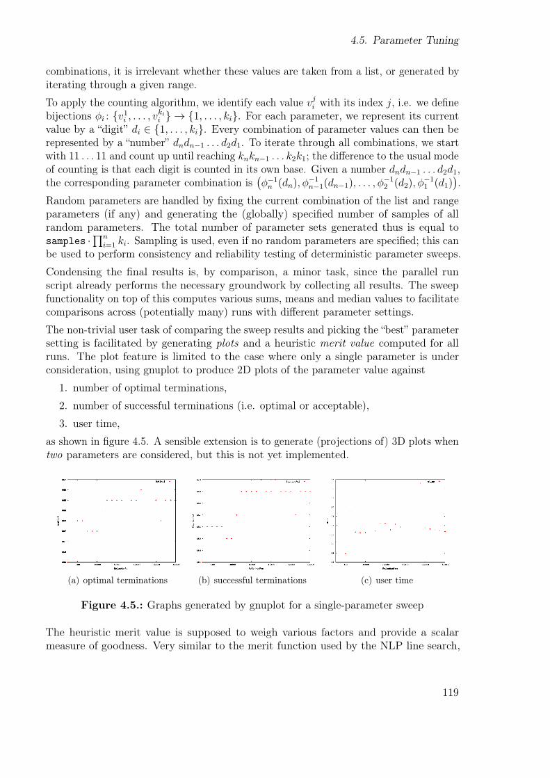
4.5. Parameter Tuning
combinations, it is irrelevant whether these values are taken from a list, or generated byiterating through a given range.
To apply the counting algorithm, we identify each value vji with its index j, i.e. we deőne
bijections φi : {v1i , . . . , vkii } → {1, . . . , ki}. For each parameter, we represent its currentvalue by a łdigitž di ∈ {1, . . . , ki}. Every combination of parameter values can then berepresented by a łnumberž dndn−1 . . . d2d1. To iterate through all combinations, we startwith 11 . . . 11 and count up until reaching knkn−1 . . . k2k1; the diference to the usual modeof counting is that each digit is counted in its own base. Given a number dndn−1 . . . d2d1,the corresponding parameter combination is
φ−1n (dn), φ
−1n−1(dn−1), . . . , φ
−12 (d2), φ
−11 (d1)
.
Random parameters are handled by őxing the current combination of the list and rangeparameters (if any) and generating the (globally) speciőed number of samples of allrandom parameters. The total number of parameter sets generated thus is equal tosamples ·n
i=1 ki. Sampling is used, even if no random parameters are speciőed; this canbe used to perform consistency and reliability testing of deterministic parameter sweeps.
Condensing the őnal results is, by comparison, a minor task, since the parallel runscript already performs the necessary groundwork by collecting all results. The sweepfunctionality on top of this computes various sums, means and median values to facilitatecomparisons across (potentially many) runs with diferent parameter settings.
The non-trivial user task of comparing the sweep results and picking the łbestž parametersetting is facilitated by generating plots and a heuristic merit value computed for allruns. The plot feature is limited to the case where only a single parameter is underconsideration, using gnuplot to produce 2D plots of the parameter value against
1. number of optimal terminations,
2. number of successful terminations (i.e. optimal or acceptable),
3. user time,
as shown in őgure 4.5. A sensible extension is to generate (projections of) 3D plots whentwo parameters are considered, but this is not yet implemented.
(a) optimal terminations (b) successful terminations (c) user time
Figure 4.5.: Graphs generated by gnuplot for a single-parameter sweep
The heuristic merit value is supposed to weigh various factors and provide a scalarmeasure of goodness. Very similar to the merit function used by the NLP line search,
119
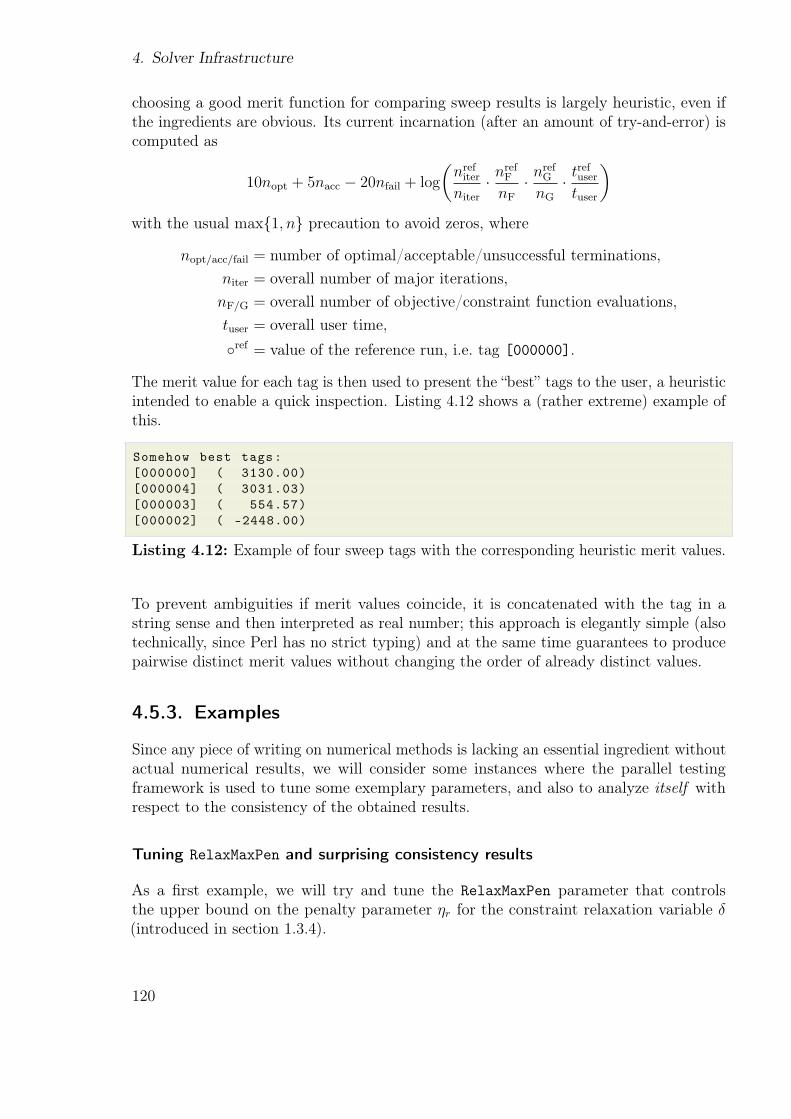
4. Solver Infrastructure
choosing a good merit function for comparing sweep results is largely heuristic, even ifthe ingredients are obvious. Its current incarnation (after an amount of try-and-error) iscomputed as
10nopt + 5nacc − 20nfail + log
nrefiter
niter
· nrefF
nF
· nrefG
nG
· trefuser
tuser
with the usual max{1, n} precaution to avoid zeros, where
nopt/acc/fail = number of optimal/acceptable/unsuccessful terminations,
niter = overall number of major iterations,
nF/G = overall number of objective/constraint function evaluations,
tuser = overall user time,
◦ref = value of the reference run, i.e. tag [000000].
The merit value for each tag is then used to present the łbestž tags to the user, a heuristicintended to enable a quick inspection. Listing 4.12 shows a (rather extreme) example ofthis.
Somehow best tags:
[000000] ( 3130.00)
[000004] ( 3031.03)
[000003] ( 554.57)
[000002] ( -2448.00)
Listing 4.12: Example of four sweep tags with the corresponding heuristic merit values.
To prevent ambiguities if merit values coincide, it is concatenated with the tag in astring sense and then interpreted as real number; this approach is elegantly simple (alsotechnically, since Perl has no strict typing) and at the same time guarantees to producepairwise distinct merit values without changing the order of already distinct values.
4.5.3. Examples
Since any piece of writing on numerical methods is lacking an essential ingredient withoutactual numerical results, we will consider some instances where the parallel testingframework is used to tune some exemplary parameters, and also to analyze itself withrespect to the consistency of the obtained results.
Tuning RelaxMaxPen and surprising consistency results
As a őrst example, we will try and tune the RelaxMaxPen parameter that controlsthe upper bound on the penalty parameter ηr for the constraint relaxation variable δ
(introduced in section 1.3.4).
120
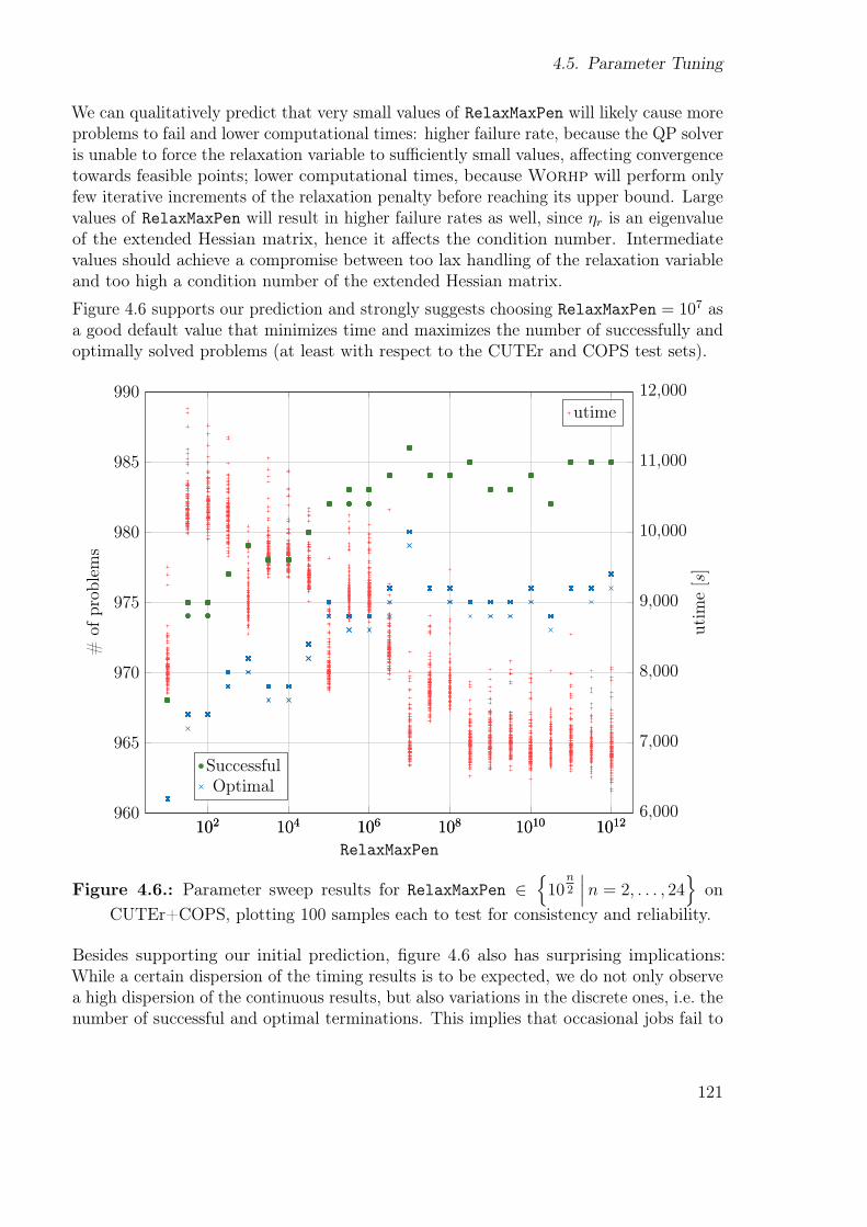
4.5. Parameter Tuning
We can qualitatively predict that very small values of RelaxMaxPen will likely cause moreproblems to fail and lower computational times: higher failure rate, because the QP solveris unable to force the relaxation variable to suiciently small values, afecting convergencetowards feasible points; lower computational times, because Worhp will perform onlyfew iterative increments of the relaxation penalty before reaching its upper bound. Largevalues of RelaxMaxPen will result in higher failure rates as well, since ηr is an eigenvalueof the extended Hessian matrix, hence it afects the condition number. Intermediatevalues should achieve a compromise between too lax handling of the relaxation variableand too high a condition number of the extended Hessian matrix.
Figure 4.6 supports our prediction and strongly suggests choosing RelaxMaxPen = 107 asa good default value that minimizes time and maximizes the number of successfully andoptimally solved problems (at least with respect to the CUTEr and COPS test sets).
102 104 106 108 1010 10126,000
7,000
8,000
9,000
10,000
11,000
12,000
RelaxMaxPen
utim
e[s]
utime
102 104 106 108 1010 1012960
965
970
975
980
985
990
#of
prob
lem
s
SuccessfulOptimal
Figure 4.6.: Parameter sweep results for RelaxMaxPen ∈
10n2
n = 2, . . . , 24
onCUTEr+COPS, plotting 100 samples each to test for consistency and reliability.
Besides supporting our initial prediction, őgure 4.6 also has surprising implications:While a certain dispersion of the timing results is to be expected, we do not only observea high dispersion of the continuous results, but also variations in the discrete ones, i.e. thenumber of successful and optimal terminations. This implies that occasional jobs fail to
121
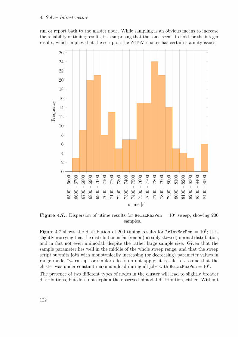
4. Solver Infrastructure
run or report back to the master node. While sampling is an obvious means to increasethe reliability of timing results, it is surprising that the same seems to hold for the integerresults, which implies that the setup on the ZeTeM cluster has certain stability issues.
6500
ś6600
6600
ś6700
6700
ś6800
6800
ś6900
6900
ś7000
7000
ś7100
7100
ś7200
7200
ś7300
7300
ś7400
7400
ś7500
7500
ś7600
7600
ś7700
7700
ś7800
7800
ś7900
7900
ś8000
8000
ś8100
8100
ś8200
8200
ś8300
8300
ś8400
8400
ś8500
0
2
4
6
8
10
12
14
16
18
20
22
24
26
utime [s]
Freq
uenc
y
Figure 4.7.: Dispersion of utime results for RelaxMaxPen = 107 sweep, showing 200samples.
Figure 4.7 shows the distribution of 200 timing results for RelaxMaxPen = 107; it isslightly worrying that the distribution is far from a (possibly skewed) normal distribution,and in fact not even unimodal, despite the rather large sample size. Given that thesample parameter lies well in the middle of the whole sweep range, and that the sweepscript submits jobs with monotonically increasing (or decreasing) parameter values inrange mode, łwarm-upž or similar efects do not apply; it is safe to assume that thecluster was under constant maximum load during all jobs with RelaxMaxPen = 107.
The presence of two diferent types of nodes in the cluster will lead to slightly broaderdistributions, but does not explain the observed bimodal distribution, either. Without
122
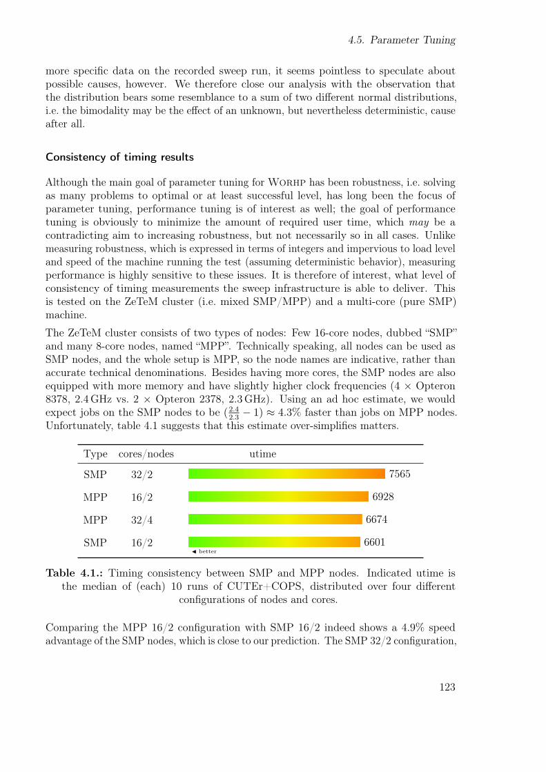
4.5. Parameter Tuning
more speciőc data on the recorded sweep run, it seems pointless to speculate aboutpossible causes, however. We therefore close our analysis with the observation thatthe distribution bears some resemblance to a sum of two diferent normal distributions,i.e. the bimodality may be the efect of an unknown, but nevertheless deterministic, causeafter all.
Consistency of timing results
Although the main goal of parameter tuning for Worhp has been robustness, i.e. solvingas many problems to optimal or at least successful level, has long been the focus ofparameter tuning, performance tuning is of interest as well; the goal of performancetuning is obviously to minimize the amount of required user time, which may be acontradicting aim to increasing robustness, but not necessarily so in all cases. Unlikemeasuring robustness, which is expressed in terms of integers and impervious to load leveland speed of the machine running the test (assuming deterministic behavior), measuringperformance is highly sensitive to these issues. It is therefore of interest, what level ofconsistency of timing measurements the sweep infrastructure is able to deliver. Thisis tested on the ZeTeM cluster (i.e. mixed SMP/MPP) and a multi-core (pure SMP)machine.
The ZeTeM cluster consists of two types of nodes: Few 16-core nodes, dubbed łSMPžand many 8-core nodes, named łMPPž. Technically speaking, all nodes can be used asSMP nodes, and the whole setup is MPP, so the node names are indicative, rather thanaccurate technical denominations. Besides having more cores, the SMP nodes are alsoequipped with more memory and have slightly higher clock frequencies (4 × Opteron8378, 2.4GHz vs. 2 × Opteron 2378, 2.3GHz). Using an ad hoc estimate, we wouldexpect jobs on the SMP nodes to be (2.4
2.3− 1) ≈ 4.3% faster than jobs on MPP nodes.
Unfortunately, table 4.1 suggests that this estimate over-simpliőes matters.
Type cores/nodes utime
SMP 32/2 7565
MPP 16/2 6928
MPP 32/4 6674
SMP 16/2 6601◭ better
Table 4.1.: Timing consistency between SMP and MPP nodes. Indicated utime isthe median of (each) 10 runs of CUTEr+COPS, distributed over four diferent
conőgurations of nodes and cores.
Comparing the MPP 16/2 conőguration with SMP 16/2 indeed shows a 4.9% speedadvantage of the SMP nodes, which is close to our prediction. The SMP 32/2 conőguration,
123

4. Solver Infrastructure
however, is signiőcantly slower than any other, and by almost 15% in comparison to theSMP 16/2 conőguration.
The most probable explanation is bandwidth contention between the (32/2 = 16) Worhp
instances on the fully loaded SMP nodes, where all other cases only run 8 instancesin parallel. Since 100 Mbit Ethernet is able to deliver signiőcantly higher throughputthan the communication for job submission and results, either TCP latency, or memorybandwidth is left to blame. In other words: The observed slowdown with 16 parallelinstances is most probably due to a saturation of a speciőc bandwidth that is not (yet)saturated by 8 instances.
Given that few problems from CUTEr, but rather more from COPS are medium-scale,the test set as a whole deőnitely puts a strain on the memory bandwidth, if by chancevarious medium-scale problems are submitted to the same node. On the other hand,CUTEr contains many problems that can be solved by Worhp in mere milliseconds,which is of similar order as typical network latencies. To conclude: While some form ofbandwidth saturation is the most likely explanation, it remains unclear which bandwidthis being saturated, without performing more extensive measurements. Preventing theSMP nodes from being fully loaded is a feasible workaround that exhibits the expectedperformance diferences between SMP and MPP nodes.
On a multi-core desktop (i.e. SMP) machine, running the sweep script in łconsistencymodež, i.e. running samples of identical parameter sets shows very little variation:
Sweep: Writing parameter files in background.
Number of sweeps: 25
*** All parameter files written ***
Using (up to) 4 threads to run 17472 problems
Tag Success Optimal Failed Iter F evl G evl utime
[000000] 661 648 11 15/8 148/11 109/5 11.34
[000001] 661 648 11 15/8 148/11 109/5 11.64
[000002] 661 648 11 15/8 148/11 109/5 11.80
[000003] 661 648 11 15/8 148/11 109/5 11.57
[000004] 661 648 11 15/8 148/11 109/5 11.73
[000005] 661 648 11 15/8 148/11 109/5 11.60
[000006] 661 648 11 15/8 148/11 109/5 11.63
[000007] 661 648 11 15/8 148/11 109/5 11.48
[000008] 661 648 11 15/8 148/11 109/5 11.46
[000009] 661 648 11 15/8 148/11 109/5 11.72
[000010] 661 648 11 15/8 148/11 109/5 11.84
[000011] 661 648 11 15/8 148/11 109/5 11.68
[000012] 661 648 11 15/8 148/11 109/5 11.80
[000013] 661 648 11 15/8 148/11 109/5 11.36
[000014] 661 648 11 15/8 148/11 109/5 11.86
[000015] 661 648 11 15/8 148/11 109/5 11.12
[000016] 661 648 11 15/8 148/11 109/5 12.06
[000017] 661 648 11 15/8 148/11 109/5 11.33
[000018] 661 648 11 15/8 148/11 109/5 11.81
[000019] 661 648 11 15/8 148/11 109/5 11.36
[000020] 661 648 11 15/8 148/11 109/5 11.70
124
4.5. Parameter Tuning
[000021] 661 648 11 15/8 148/11 109/5 11.42
[000022] 661 648 11 15/8 148/11 109/5 12.04
[000023] 661 648 11 15/8 148/11 109/5 11.55
*** All jobs sent to workers ***
[000024] 661 648 11 15/8 148/11 109/5 11.87
[000025] 661 648 11 15/8 148/11 109/5 10.99
The distribution of the utime values is reasonably close to a normal distribution (72%probability), and their standard deviation σ = 0.26 is almost two orders of magnitudesmaller than the values. The most important observation is that the last utime value isa clear outlier. This is probably due to the lower machine load in the last sweep run,which puts a smaller strain on caches and memory bandwidth.
Tuning ScaleFacObj and sweep automation
Let us now consider the ScaleFacObj parameter, which deőnes a scaling target withrespect to the objective. If this scaling mode is enabled (by the scaledObj ŕag), theobjective is scaled by the factor
c+ ..= min
1,ScaleFacObj
|1cf(x)|
,
which is updated in every major iteration. The motivation behind this scaling factor isto leave reasonably well-scaled objectives alone, while reining in the badly-scaled ones.We consider a őne-grained parameter sweep for 10−5 6 ScaleFacObj 6 105.
Since higher values cause Worhp to apply scaling to fewer of the test problems, we canqualitatively expect lower values to produce better results, if badly scaled objectives areresponsible for unsuccessful terminations with the default settings.
Considering the sweep results őgure 4.8, we can make various observations:
1. The results are subject to pronounced dispersion. One possible interpretation is thatamong the roughly 1000 test problems, few have problem conditions that tax thenumerical methods in Worhp to their limits, hence minor scaling variations maybe the decisive element between optimal, acceptable or unsuccessful termination ofthe solver.
This is a general observation in parameter sweeps: Some test problems are particularlysensitive to certain solver parameters and may show quasi-stochastic behavior in thesweep results. The set of these test problems is parameter-dependent, although someproblems (such as some instances of the palmer, the vanderm and the himmel series) areparticularly conspicuous. In our case, the dispersion width suggests that 3 or 4 problemshave this quasi-stochastic sensitivity to ScaleFacObj.
These łquasi-stochasticž test problems have proven to be problematic for the parametersweep, if computational resources are limited, and the overall sample rate is low, sincethey may suggest highly localized maxima (of successful/optimal terminations) or minima
125
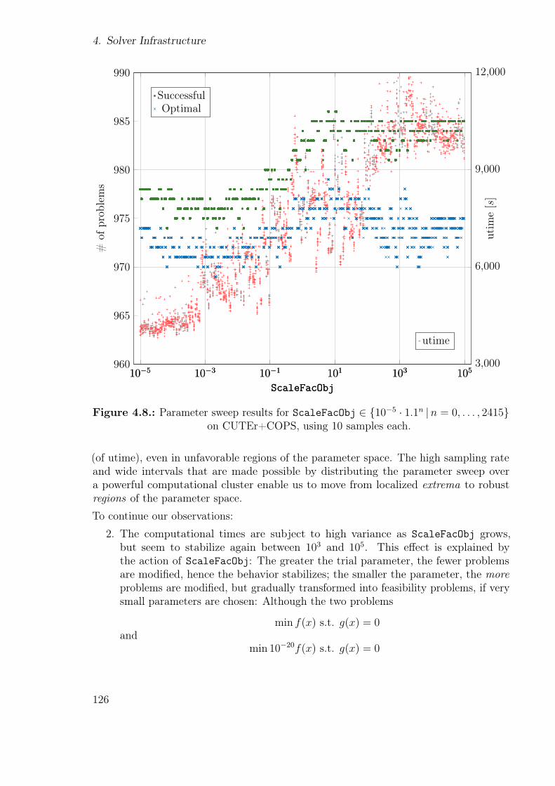
4. Solver Infrastructure
10−5 10−3 10−1 101 103 1053,000
6,000
9,000
12,000
ScaleFacObj
utim
e[s]
utime
10−5 10−3 10−1 101 103 105960
965
970
975
980
985
990
ScaleFacObj
#of
prob
lem
sSuccessfulOptimal
Figure 4.8.: Parameter sweep results for ScaleFacObj ∈ {10−5 · 1.1n |n = 0, . . . , 2415}on CUTEr+COPS, using 10 samples each.
(of utime), even in unfavorable regions of the parameter space. The high sampling rateand wide intervals that are made possible by distributing the parameter sweep overa powerful computational cluster enable us to move from localized extrema to robustregions of the parameter space.
To continue our observations:
2. The computational times are subject to high variance as ScaleFacObj grows,but seem to stabilize again between 103 and 105. This efect is explained bythe action of ScaleFacObj: The greater the trial parameter, the fewer problemsare modiőed, hence the behavior stabilizes; the smaller the parameter, the moreproblems are modiőed, but gradually transformed into feasibility problems, if verysmall parameters are chosen: Although the two problems
min f(x) s.t. g(x) = 0and
min 10−20f(x) s.t. g(x) = 0
126
4.5. Parameter Tuning
are equivalent from a theoretical point of view, the second one degenerates into afeasibility problem g(x) = 0 when solved numerically. It is therefore the łmiddležregion, where many test problems are afected by the parameterÐand hence showvarianceÐ, but whose objective still has numerical inŕuence.
3. We can observe two local maxima with respect to optimal & successful terminations,and one (boundary-)minimum of the utime values. Had we added additionalłintelligencež, in form of support vector machines or global optimization techniques,to the sweep script to automatically identify optimal parameters, it might return10−5 as optimal choice. However, as explained earlier, this choice would essentiallytransform optimization problems into feasibility problems, which is clearly againstthe user’s intentions.
Gathering and incorporating all observations, the current default of RelaxMaxPen = 101
is a suitable choice (at least with respect to the test set), since it hits the globalmaximum of optimal & successful terminations, and does not interfere with thoroughlywell-scaled problems. The timing results for this region are hard to interpret throughthe high dispersion, but on average lie well below the maximum times reached aroundRelaxMaxPen = 103.
4.5.4. Conclusions
The parameter sweep was introduced to enable parameter tuning, both generic andproblem-speciőc. It is intended to somewhat ease the burden of requiring deep knowledgeof both the optimizer and the application to be able to tune solver parameters. While ithas yet to be applied by users, it is not intended as developer-exclusive tool; running thesweep script is suiciently simple to allow wider use in any case, but the interpretationof the results is not necessarily as simple as the graphs suggest. If users are applyingthe parameter sweep to self-chosen test sets, we can assume, however, that they are ableto interpret the results and would therefore not łfall for trapsž such as the potentiallymisleading result of the RelaxMaxPen sweep discussed earlier.
This anticipates one major conclusion: While the parameter sweep is simple to run,blindly trusting its results can be dangerous, which is the reason why the sweep script hasdeliberately not been equipped with additional intelligence to automate the parameterchoice: The sweep technique still requires a reŕecting user to scrutinize its results.
The second conclusion concerns consistency and reliability: As the multi-core testindicates, running the sweep script on a (preferably unloaded) modern desktop machineyields reliable results that are very consistent across repeated runs; the only observedvariation concerns the time measurements. To achieve higher accuracy here, a small (2ś5)number of samples can be used in addition to the (deterministic) parameter variations tocalculate a median of the timing results as highly reliable measure.
As the examples suggest, conditions are slightly worse on the ZeTeM cluster, caused byunreliable nodes with randomly dying slaves and currently unexplained issues that result
127
4. Solver Infrastructure
in high dispersion of timing results. Since even the integer measurements show variation,sweep runs on the cluster always have to use sampling to achieve reliable results. Ifrobustness is the major concern, a rather small number of samples can already guardagainst false results: If we assume a probability of 10−4 (1 in 1000) for a test problemto fail because of technical problems (in reality, it is probably still lower), a single runof CUTEr+COPS has a 1− (1− 10−4)988 ≈ 9.4% probability of returning a false resultdue to one or more technical failures; this is uncomfortably high. However, using 2 or 3samples, we can lower the probability of all test runs returning a false result to 0.89%and 0.083%, respectively, which seems acceptable.
Achieving comparably reliable timing results on the cluster seems to require many moresamples, considering the dispersion observed in őgure 4.7, which is not even normallydistributed (probability < 4.2 · 10−7). It still seems sensible to use the median value ofthe results of multiple samples, instead of the minimum, since deviations are presentin both directions, for instance if a slave with a long-running problem dies immediatelyafter starting it.
All in all, the parallel parameter sweep is a powerful tool, although it requires some carein interpreting its results. The reliability of its results is excellent on multi-core machines,and can be increased to satisfactory levels on the cluster by the use of sampling. Itis unique with its capability of “optimizing the optimizer”, which has likely never beenconsidered for NLP solvers as systematically as described here.
4.6. Future directions for testing
When viewed from a software engineering angle, the current testing regime of Worhp
is very narrowly focused on performance and less on veriőcation and validation in thesoftware-technical sense. The current form of testing could be regarded as a combinationof system testing, which usually is the last or last-but-one step in formalized softwaretesting, and performance testing. With continued development and maintenance ofWorhp, it will be sensible to add more software-engineering oriented forms of testing:unit tests8 perform freestanding tests on single routines or modules, such as Worhp’s CSmodule that provides routines for handling sparse matrices. This form of testing is easierto perform than system testing, since each module has only few, well-deőned functionsof lower complexity than the overall system, and thus requires fewer or simpler tests toexhaustively test it for defects.
Continuous Integration (CI) is a quality assurance technique that merits partial inclusioninto the development process. Given the existing run script for providing test results andthe conőguration and build system, an initial setup requires only a continuous integrationserver that monitors the code repository (Subversion[57] in Worhp’s case) and triggerstest and build runs under certain conditions ś usually at every commit, when followingthe CI rules to the letter. Examples of such CI servers are Jenkins[44], written in Java,
8Engineers might call this “module-in-the-loop”
128
4.6. Future directions for testing
but easily applicable to other łeco-systemsž by plugins, and bitten[65], based on trac[66],both written in Python.
Besides extending the testing approach to new technical forms of testing, it is highlynecessary to extend the test sets by new problems, problem classes and using diferentinterfacesÐthe CUTEr and COPS tests are currently exclusively run through the AMPLinterface. This may obscure existing weaknesses of other interfaces or Worhp’s numericaland algorithmic core, since AMPL provides analytic derivatives, whose precision dependsonly on the machine precision and the math library, and internally simpliőes the problem,removing variables or constraints. Formerly existing problems in handling őxed variableswere only discovered through an application based on the MATLAB interface, sinceAMPL removes these.
Extending the test set with new test problems, and most importantly, beyond AMPL istherefore critical for Worhp’s intended use as a general-purpose, robust NLP solver.
129


AppendixA
Examples
A.1. Bypassing const-ness
These two examples use C to demonstrate bypassing a const qualiőer on a routineargument by changing it through a global pointer.
1 #include <stdio.h>
2 #include <stdlib.h>
3
4 /* Used for global access to n in main */
5 static int *np;
6 void routine1(const int n);
7 void routine2(const int n);
8
9 int main (void) {
10 int n = 42; np = &n;
11 routine1(n);
12 exit(EXIT_SUCCESS );
13 }
14 void routine1(const int n) {
15 routine2(n);
16 printf("After routine2: n = %d\n", n);
17 }
18 void routine2(const int n) {
19 (*np)++; /* Increment n */
20 printf("After increment: n = %d\n", n);
21 }
Listing A.1: Example for bypassing const-ness and call-by-value.
In example listing A.1, routine2 needs to use a global pointer to (in a way) changeits argument n, since it inherited its const-ness from routine1 and we are unwilling tochange the whole calling hierarchy.
131
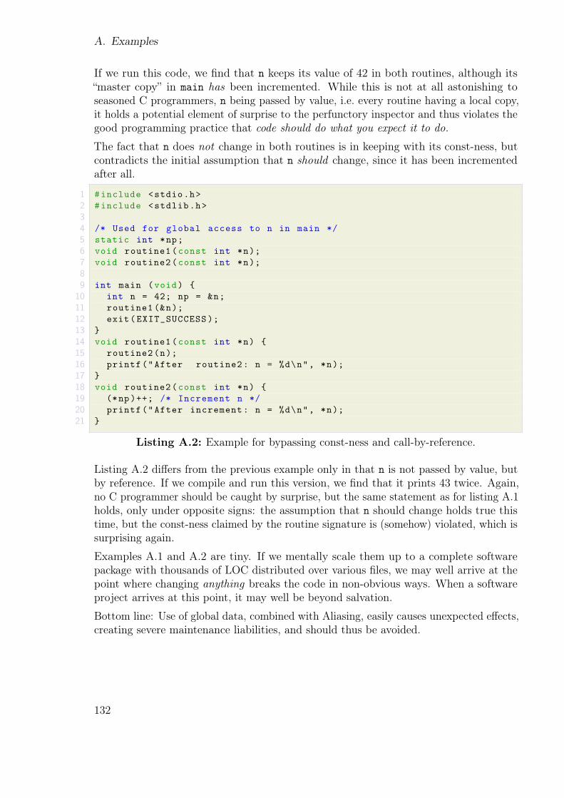
A. Examples
If we run this code, we őnd that n keeps its value of 42 in both routines, although itsłmaster copyž in main has been incremented. While this is not at all astonishing toseasoned C programmers, n being passed by value, i.e. every routine having a local copy,it holds a potential element of surprise to the perfunctory inspector and thus violates thegood programming practice that code should do what you expect it to do.
The fact that n does not change in both routines is in keeping with its const-ness, butcontradicts the initial assumption that n should change, since it has been incrementedafter all.
1 #include <stdio.h>
2 #include <stdlib.h>
3
4 /* Used for global access to n in main */
5 static int *np;
6 void routine1(const int *n);
7 void routine2(const int *n);
8
9 int main (void) {
10 int n = 42; np = &n;
11 routine1 (&n);
12 exit(EXIT_SUCCESS );
13 }
14 void routine1(const int *n) {
15 routine2(n);
16 printf("After routine2: n = %d\n", *n);
17 }
18 void routine2(const int *n) {
19 (*np)++; /* Increment n */
20 printf("After increment: n = %d\n", *n);
21 }
Listing A.2: Example for bypassing const-ness and call-by-reference.
Listing A.2 difers from the previous example only in that n is not passed by value, butby reference. If we compile and run this version, we őnd that it prints 43 twice. Again,no C programmer should be caught by surprise, but the same statement as for listing A.1holds, only under opposite signs: the assumption that n should change holds true thistime, but the const-ness claimed by the routine signature is (somehow) violated, which issurprising again.
Examples A.1 and A.2 are tiny. If we mentally scale them up to a complete softwarepackage with thousands of LOC distributed over various őles, we may well arrive at thepoint where changing anything breaks the code in non-obvious ways. When a softwareproject arrives at this point, it may well be beyond salvation.
Bottom line: Use of global data, combined with Aliasing, easily causes unexpected efects,creating severe maintenance liabilities, and should thus be avoided.
132
List of terms
Aliasing describes the situation where a single piece of data (in memory) can be accessedthrough two or more pointers. The fact that Fortran forbids aliasing by defaultaccounts for its high performance, since it allows compilers to make aggressive useof caching and greatly simpliőes dependency analysis. In contrast, C allows aliasingby default, hence C compilers have to work more conservatively to guarantee dataconsistency. 133
AMPL is A Modeling Language for Mathematical Programming[22]. It allows to formu-late optimization problems in an intuitive language closely resembling mathematicalnotation, and uses symbolic operations to simplify the problem and provide exact(to machine precision) derivatives. 95, 96, 104, 107, 110, 137, 143
Application Binary Interface deőnes the interface between programs or libraries onthe assembler level, i.e. byte order (see endianness), stack convention, etc.. Softwarecompatibility on the ABI level is often desirable to allow for simple upgrade paths,but challenging, since there are signiőcant diferences between diferent compilers(or versions of them) and platforms. 145
Application Programming Interface in our sense is the deőnition of types and func-tions used to communicate with a given piece of software, often a program library.Software development diferentiates between stable and evolving APIs, where theőrst remains static or at least downwards-compatible over various versions, whereasthe latter may change in incompatible ways between diferent versions of the soft-ware. The GNOME libxml2[73] is an example of a stable API, while the Linuxkernel’s API is deliberately left unstable. 139, 145
ASL supposedly an acronym for łAMPL solver libraryž provides the back-end libraryfor hooking NLP (or other) solvers to AMPL. It is available from http://www.
netlib.org/ampl/solvers. 104
AutoGen łis a tool designed to simplify the creation and maintenance of programs thatcontain large amounts of repetitious text. It is especially valuable in programsthat have several blocks of text that must be kept synchronized.ž [47]. AutoGen isbased on Scheme, using the guile[5] library. It is used by Worhp to generate a
133
List of terms
large portion of the data structure-related code. 69, 95
barrier is a concept used in multi-threaded software. A barrier is a code point that hasto be reached by a set of threads before the program continues; it causes fasterthreads to wait for the slower threads to łcatch upž. Barriers are typically usedwhen results from multiple threads are condensed. 113
bash the Bourne-again shell is the standard shell on many current GNU/Linux systems.It is mostly compatible with the older Bourne Shell sh introduced with Unix V7,but also adopted some features of the Korn-Shell ksh and the C-Shell csh. 83,110, 111
BLAS the Basic Linear Algebra System deőnes a set of routines that perform basicoperations on vectors and matrices for higher-level code to rely on, so that eacharchitecture can provide (in the engineering sense) optimized versions. Routines aregrouped into levels 1ś3 according to their operands (scalar-vector, matrix-vectorand matrix-matrix). 39, 95
CamelCase is a convention for concatenating words by capitalizing the őrst letter of everyinterior word, as in CamelCase or computeThisNumber. Using underscores to con-nect words (as in compute_this_number) can be thought of as the complementaryconvention. 47
Continuous Integration is a form of software quality insurance developed that focuseson tightly coupling small, incremental changes with highly automated testing andbuilding infrastructure. Its central aim is to expose conŕicts and errors introducedby changes early though continued automated building and testing of the softwareunder development. 129, 145
COPS the Constrained Optimization Problem Set is a collection of large-scale, whosełprimary purpose [. . . ] is to provide diicult test cases for optimization software.Problems in the current version of the collection come from ŕuid dynamics, popula-tion dynamics, optimal design, mesh smoothing, and optimal control.ž. COPS 3.0is documented in [16, 17]. 107
CUTEr an acronym for łCUTE revisitedž is a collection of over 1,100 optimizationproblems in SIF format that serves the purpose of providing a standard set ofproblems to test and compare optimization codes. Worhp is benchmarked with a920-problem set that contains roughly 750 problems of the complete collection thatis documented at [56]. 95, 107, 111
Debugging derived from the term łbugž, which is nowadays used to describe any kind ofdefect in software. Its origin lies in Harvard, where on September 9, 1947, engineersworking on the Mark II computer found a moth stuck in relay #70, causing anarithmetic test to fail. Grace Murray Hopper is reported to have coined the termłdebuggingž on this occasion. 107
134
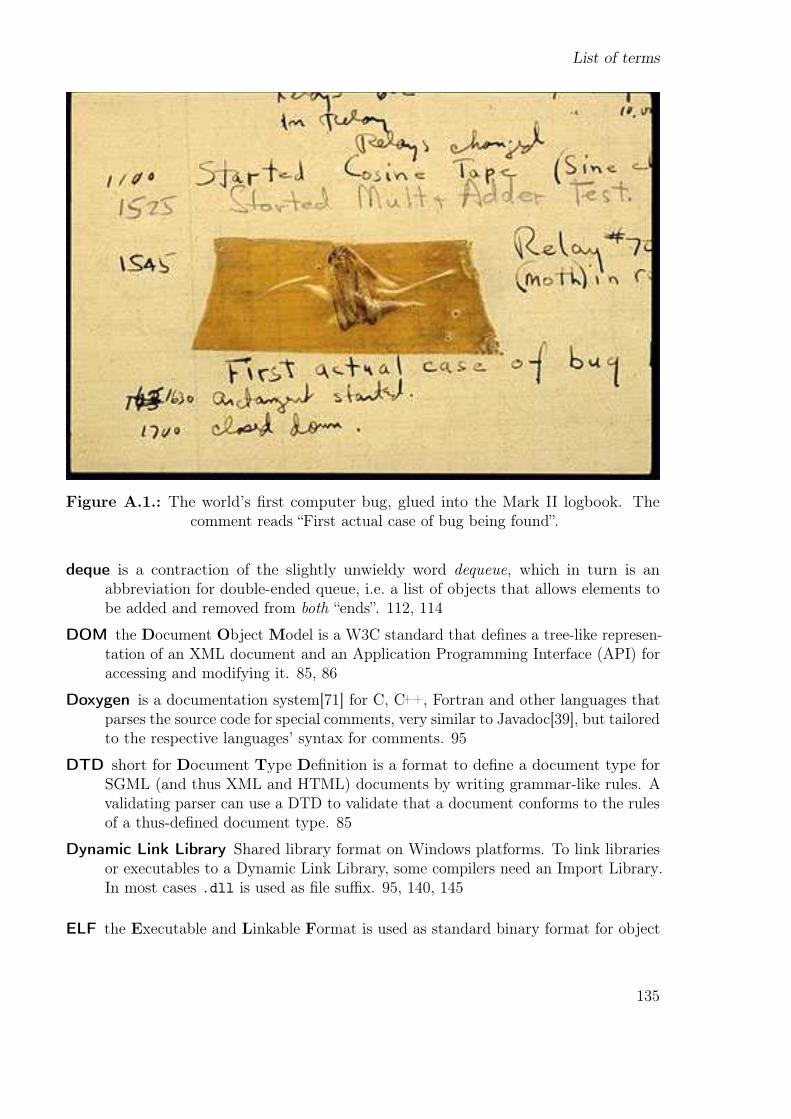
List of terms
Figure A.1.: The world’s őrst computer bug, glued into the Mark II logbook. Thecomment reads łFirst actual case of bug being foundž.
deque is a contraction of the slightly unwieldy word dequeue, which in turn is anabbreviation for double-ended queue, i.e. a list of objects that allows elements tobe added and removed from both łendsž. 112, 114
DOM the Document Object Model is a W3C standard that deőnes a tree-like represen-tation of an XML document and an Application Programming Interface (API) foraccessing and modifying it. 85, 86
Doxygen is a documentation system[71] for C, C++, Fortran and other languages thatparses the source code for special comments, very similar to Javadoc[39], but tailoredto the respective languages’ syntax for comments. 95
DTD short for Document Type Deőnition is a format to deőne a document type forSGML (and thus XML and HTML) documents by writing grammar-like rules. Avalidating parser can use a DTD to validate that a document conforms to the rulesof a thus-deőned document type. 85
Dynamic Link Library Shared library format on Windows platforms. To link librariesor executables to a Dynamic Link Library, some compilers need an Import Library.In most cases .dll is used as őle suix. 95, 140, 145
ELF the Executable and Linkable Format is used as standard binary format for object
135
List of terms
code, libraries and executables on many Linux and Unix platforms, replacing theolder a.out and COFF formats. An ELF object can be examined with several tools,among them readelf and objdump. 62, 104, 105, 143
endianness is a property of a processor architecture that describes the bit storage orderof integers. Big-endian architectures save the MSB őrst (at the lowest bit of aword) and the LSB last (at the highest bit of a word), whereas little-endian has theexact opposite storage order. Arabic numbers, for instance, are written down inbig-endian order, whereas the German ordering of dates as DD.MM.YYYY can bethought of as little-endian. The Intel x86(-64) architecture is little-endian, whileSPARC and PowerPC are historically big-endian (actually bi-endian nowadays,supporting both modes). 57, 137
HSL (formerly the Harwell Subroutine Library) is a collection of threadsafe ISO Fortrancodes for large scale scientiőc computation [34]. 95
Import Library Specialized static library on Windows platforms needed by the linker tolink against a Dynamic Link Library. Native Windows tools use the .lib suix,but the MinGW-related tools also use .dll.a. 139
Ipopt łis an open-source solver for large-scale nonlinear continuous optimization. It canbe used from modeling environments, such as AMPL, GAMS, or Matlab, and it isalso available as callable library with interfaces to C++, C, and Fortran. Ipopt usesan interior point method, together with a őlter linear search procedurež[74]. Thesolver Ipopt is presented in [75]. 38
JSON the JavaScript Object Notation[13] is a standard for serializing JavaScript objects,i.e. it deőnes a mapping between objects and a string representation of them. JSONsupports numeric, logical and string data types and used C-like { } notation fordenoting hierarchies. 50
LAPACK the Linear Algebra Package provides an extensive set of higher-level routinesfor łsolving systems of simultaneous linear equations, least-squares solutions oflinear systems of equations, eigenvalue problems, and singular value problemsž. 95
LISP is a functional language based on λ-calculus. LISP is an acronym for ListProcessing, but the humorous Lots of Irritating Superfluous Parentheses is re-garded a more appropriate description by some. (X)emacs is an example of awell-known application written in a LISP dialect called Emacs Lisp. 143
locale deőnes the country-/language-speciőc conventions for date and time format,number representation (in particular decimal point), currency symbol, time zoneand others. 87
magic number is a derogatory term for the use of literal numbers in code whose jus-tiőcation is not obvious. Examples are conditionals like if (iFlag == 31415)
136
List of terms
(where 31415 should be replaced by a descriptive constant), dimensions like char
string[13] or even arithmetic like i = 60*j; since i and j are completely nonde-scriptive, does 60 describe the number of seconds in a minute, of years betweenthree successive Great Conjunctions of Jupiter and Saturn or of carbon atoms in abuckyball? One main criticism of magic numbers is their burden on maintenance,since refactoring named constants is trivial against őnding and replacing (thecorrect!) number literals in extensive code. 47
Massively Parallel Processing abbreviated as MPP describes parallel computing onmany processors that do not have shared, but distributed memory, i.e. the processorsare coupled loosely by network or similar connections. Parallel programming thatuses explicit message passing, such as MPI, is required on MPP architectures. 143,145
MATLAB is an extensive development environment for numerical algorithms[49]. Itoperates numerically on matrices and vectors and is very suitable for prototypingand quick visualization, but lacks the performance of compiled languages. 96
METIS is a set of routines for partitioning graphs, partitioning őnite element meshes,and producing őll-reducing orderings for sparse matrices[43, 50]. 95
MinGW Minimalist GNU for Windows[52] is a project that ports part of the GNUtoolchain to Windows, which includes (a subset of) the Windows API, compilersfrom the GCC and binutils. It allows the creation of native Windows binaries, butdoes explicitly not emulate a POSIX-like environment, like cygwin does. 140
name mangling is the mapping of a function name in the source code to its assem-bler name in the generated object code. For C, the mapping is usually direct,while C++ employs complex mappings to handle polymorphism on the linkerlevel (example: long foo(std::vector<double> &v, size_t n) is mangled to_Z3fooRSt6vectorIdSaIdEEm by g++). Fortran compilers also mangle functionand subroutine names in a vendor-speciőc way. 62
Nonlinear Programming The Name of the Game: Nonlinear Programming is the pro-cess of minimizing a smooth (nonlinear) objective function subject to smooth(nonlinear) equality and inequality constraints, usually by iterative numerical meth-ods like Worhp. 145
Object-oriented Programming is a programming paradigm popularized with the ad-vent of C++, although its inception dates back many years before that. Its maindistinction from other programming paradigms, such as functional or imperative,is the focus on data encapsulated in objects with operations deőned on them.Important concepts are inheritance, polymorphism and encapsulation. 38, 145
Perl is an extensive scripting language, initially designed as łgluež language with emphasison text processing, but nowadays extended by various modules to a general-purposelanguage suitable for many applications. One of its distinctive features is its rather
137
List of terms
large body of keywords that purposefully includes redundancies (unless(cond) isa graphic example of this, intended as more intuitive alternative to if(not(cond))
that needs to be used in other languages). Perl is often characterized by the łthereis more than one way to do itž (TIMTOWTDI) paradigm, which facilitates writingPerl programs but may result in code that is hard to understand. Perl also followsthe so-called łdo what I meanž-approach for interpreting language constructs innon-surprising ways. 69, 110, 142
PVFS originally named Parallel Virtual File System[61] is a őle system for distributedcomputing focused on delivering high performance and scalability to petabytedimensions. 111
Python is a universal, multi-paradigm programming language with a strong focus onclarity, readability and expressiveness, backed by a very extensive standard library.Distinct features of Python are signiőcant whitespace (blocks are deőned by in-dention) and the small size of its set of builtin functionality and keywords. Thelanguage philosophy is somewhat opposite to Perl in providing a minimalistic,redundancy-free, easily extensible language that allows (and encourages) a single,clear, łcanonicalž implementation of any given problem. Python is therefore consid-ered as very suitable for teaching, but in contrast to other didactic programminglanguages, is also actually being used for serious software projects. 69
R is a free, open-source system for statistical computation and visualization, documentedin [58]. 83
Ragel is a state machine compiler that targets languages like C, C++, Java and Ruby.It uses a regular language to deőne a grammar, and to embed actions to performduring the scanning/parsing process. Ragel then creates free-standing code thatdeőnes a őnite-state machine to scan/parse the deőned grammar. 85
Regression Testing is a test method applicable to software producing output that cansomehow be veriőed or checked against a reference, with the aim to identify andcorrect modiőcations to the software that cause it to fail on inputs, which werehandled correctly before. A regression test is performed by (usually automatically)iterating over a set of inputs and verifying the outputs, e.g. by comparing againstsome reference output. Regression testing is most powerful, if for every identiőeddefect an input to trigger it is added to the test set ś this approach can veryefectively prevent the re-surfacing of bugs that have been őxed before. The GCC isa noticeable example of a software package that relies heavily on regression testingfor developing and accepting bugőxes: the test suite of GCC 4.6 consists of morethan 40,000 individual pieces of code. 107
Reverse Communication is a software architecture convention that places tasks usuallyperformed in the bowels of a software package (the callee) back into the callershands, e.g. the evaluation of a function: instead of implementing a function andproviding a pointer to it to the callee, who then calls the function at his owndisposal, the caller, when prompted by the callee, is given control, performs the
138
List of terms
function’s action and hands the control back to the callee. This reversal of theusual interaction between caller and callee has coined the term. 32, 41, 43, 66, 145
Scheme is a LISP dialect with a minimalistic design philosophy[67], aimed at allowingenough ŕexibility and providing extension tools to extend the language to the usersneeds, rather than deőning an exhaustive set of language features. 69, 95, 137
sed short for stream editor is a stream-oriented text processor on unixoid platforms(although ports to other platforms, such as Windows exist). It uses a very concisesyntax for searching, replacing, stack manipulations and such, which actually makeit Turing-complete; accomplished sed programmers have implemented a calculator,a Linux to Unix assembler converter, or Sokoban(!) using sed. 69, 104
SIF the Standard Input Format is a text format for specifying linear, quadratic andnonlinear optimization problems, closely linked with the NLP solver LANCELOT[12]that is based on SIF as input format, and the MPS format for linear problems, ofwhich it is a superset. A sifdecode tool is available to generate FORTRAN codefrom SIF őles, which can be used to solve SIF-encoded problems with other solvers.In contrast to AMPL or similar formats, SIF is highly non-intuitive, requiring theproblem to be formulated as a high-level structural representation. The format isdescribed in [7]. 107
SuperLU is a general purpose library for the direct solution of large, sparse, nonsymmetricsystems of linear equations on high performance machines[15, 48]. 95, 96
symbol versioning is an extension to ELF that allows to annotate symbols (i.e. functions)in a shared library with a version, and to provide diferent versions of one symbolto a caller. It is used to retain backwards-compatibility even if the functionality ofexisting functions changes. The GNU libc makes ample use of symbol versioning,in order to support existing binaries without recompilation after libc updates. 51
Symmetric Multi-Processing abbreviated as SMP describes parallel computing onsystems where all processors have access to a single (large) amount of shared memory,hence communication between processors only requires locks or semaphores, butdata does not have to be passed around in messages, as required by MassivelyParallel Processing. OpenMP is a typical choice for programming on SMP machines.145
sys time is the subset of a computer’s CPU time that is used by the kernel on behalf ofa process, and as such is complementary to user time. The sys time should usuallybe much lower than the user time for a numerical application, unless it performsintense I/O operations. The total CPU time used by and for a given process is thesum of user and sys time. 114
Unified Solver Interface is a marketing-compatible term referring to the uniform (opt,
wsp, par, cnt) interface of many Worhp routines. 32, 38, 40, 146
139
List of terms
unit of least precision is the absolute spacing between two consecutive ŕoating pointnumbers, abbreviated as ulp. It is related to the machine epsilon, which describesthe same concept normalized to the ŕoating point number 1.0. The IEEE standarddictates that the result of elementary arithmetic operations with ŕoating pointnumbers be within 0.5 ulp of the exact result. 146
user time is the subset of a computer’s CPU time that the kernel allocates to a process.It excludes time used by the kernel on behalf of this process, e.g. for őle operations,and the time spent sleeping, when the kernel allocated CPU time to other processes.For single-thread processes, user time is always less than wall time, since it sharesthe CPU with the kernel and other processes. 107, 114, 143, 144
valgrind is an extensive and invaluable debugging and proőling tool for Linux. It usesdynamic recompilation of binary program code into an internal representation toenable a very wide range of possible diagnostics, including memory debugging, heapand cache proőling, diagnosing race conditions between threads and producing callgraphs[53, 6, 54, 55]. 70, 84
wall time is the physical time used by a process, such as a stopwatch operated by theuser (or the clock on the wall) would measure it. While it gives an indication ofthe perceived speed of a process, it is misleading on machines under load, wheremany active processes compete for CPU time and where the user time is a moreappropriate way of measuring and comparing (performance) timings on computers.For single-thread processes, wall time is a strict upper bound for the user time, butmulti-threaded processes usually reverse this order, since user time (at least onLinux systems) is cumulative for multiple CPUs. 114, 144
Workspace Management Table 2D integer table used by Worhp to track start/end-indices and sizes of Workspace Slices. 79, 146
Workspace Slice Array slice of one of Worhp’s large workspace arrays.. 144
XML the eXtensible Markup Language is a Unicode-based markup language for creatingmachine-readable documents[8]. An XML document has a tree-structure and isorganized by annotating its content with tags and attribute-value pairs. 50, 96, 139
YAML Ain’t Markup Language[19] is a recursive acronym for a plain-text serializationlanguage. It supports key-value pairs, lists, associate arrays and hierarchies, whichit denotes by indention, and distinguished between integer, ŕoat, boolean and stringdata. 50
ZeTeM cluster is a cluster of 36 computing nodes (4 SMP nodes with 16 cores + 32MPP nodes with 8 cores) with a total of 320 Opteron cores and a theoretical peakperformance in the order of 100 GFlops. TORQUE[36] is used as resource managerand MOAB[35] as job scheduler. 111, 112, 123, 124
140
List of acronyms
ABI Application Binary Interface. 89
API Application Programming Interface. 41, 89, 139
CI Continuous Integration. 129
DAG directed acyclic graph. 94
DLL Dynamic Link Library. 95, 96
FSM őnite-state machine. 85
GCC GNU Compiler Collection. 95, 106, 107, 141, 142
GNU GNU’s not Unix. 69, 92, 94, 98, 99, 104, 141
IWMT Integer Workspace Management Table. 79
LOC Lines of code. 133
LSB least signiőcant bit. 57, 140
MPP Massively Parallel Processing. 124
MSB most signiőcant bit. 57, 140
NLP Nonlinear Programming. 38
OOP Object-oriented Programming. 38, 42
RC Reverse Communication. 32, 46, 66
RWMT Real Workspace Management Table. 79
SMP Symmetric Multi-Processing. 124
141

List of acronyms
SQP Sequential Quadratic Programming. 1
ulp unit of least precision. 50
USI Uniőed Solver Interface. 32, 38, 40, 44
WMT Workspace Management Table. 79
142
Bibliography
[1] David Abrahams and Vladimir Prus, Boost.Build, http://www.boost.org/doc/tools/build/.
[2] GNU Automake, http://www.gnu.org/software/automake/.
[3] Ned Batchelder, cog, http://nedbatchelder.com/code/cog/.
[4] Bryan Blackburn, Joshua Root, Rainer Müller, Ryan Schmidt, et al., MacPorts,http://www.macports.org/.
[5] Jim Blandy, Greg Harvey, et al., Guile, the GNU Ubiquitous Intelligent Languagefor Extensions, http://www.gnu.org/software/guile/.
[6] Michael D. Bond, Nicholas Nethercote, Stephen W. Kent, Samuel Z. Guyer,and Kathryn S. McKinley, Tracking bad apples: Reporting the origin of null andundefined value errors, Proceedings of the ACM SIGPLAN International Conferenceon Object-Oriented Programming, Systems, Languages and Applications (OOPSLA2007) (Montreal, Canada), October 2007, pp. 405ś422.
[7] I. Bongartz, A.R. Conn, N.I.M. Gould, and Ph.L. Toint, CUTE: Constrained andUnconstrained Testing Environment, ACM Transactions on Mathematical Software21 (1995), no. 1, 123ś160.
[8] Tim Bray, Jean Paoliand C. M. Sperberg-McQueen, Eve Maler, and François Yergeau,Extensible Markup Language (XML) 1.0, http://www.w3.org/TR/REC-xml/.
[9] C. G. Broyden, The convergence of a class of double-rank minimization algorithms.II. The new algorithm, J. Inst. Math. Appl. 6 (1970), 222ś231.
[10] Christof Büskens, Optimization Methods and Sensitivity Analysis for Optimal ControlProblems with Control and State Constraints, Dissertation, Universität Münster,Münster, 1998.
[11] , Real-Time Optimization and Real-Time Optimal Control of Parameter-Perturbed Problems, Professorial dissertation, Universität Münster, Münster, 2002.
[12] A.R. Conn, N.I.M. Gould, and Ph.L. Toint, LANCELOT, A Fortran Package forLarge-Scale Nonlinear Optimization (Release A), Springer Series in ComputationalMathematics, no. 17, 1992.
143
Bibliography
[13] D. Crockford, JavaScript Object Notation (JSON), http://www.json.org/.
[14] E. Cuthill and J. McKee, Reducing the bandwidth of sparse symmetric matrices,ACM ’69 Proceedings of the 1969 24th national conference (New York, NY, USA),1969, pp. 157ś172.
[15] James Demmel, Stanley C. Eisenstat, John Gilbert, Xiaoye S. Li, and Joseph W. H.Liu, A supernodal approach to sparse partial pivoting, SIAM J. Matrix Analysis andApplications 20 (1999), no. 3, 720ś755.
[16] E. Dolan and J. Moré, Benchmarking Optimization Software with PerformanceProfiles, Mathematical Programming 91 (2002), 201ś213.
[17] E. Dolan, J. Moré, and T. Munson, Optimality measures for performance profiles,SIAM Journal on Optimization 16 (2006), 891ś909.
[18] Paul Eggert and Eric Blake, GNU Autoconf, http://www.gnu.org/software/
autoconf/.
[19] Clark C. Evans, YAML Ain’t Markup Language (YAML), http://www.yaml.org/.
[20] R. Fletcher, A new approach to variable metric algorithms, Comput. J. 13 (1970),no. 3, 317ś322.
[21] Anders Forsgren, Philip E. Gill, and Margaret H. Wright, Interior methods fornonlinear optimization, SIAM Review 44 (2002), no. 4, 525âĂŞś597.
[22] Robert Fourer, David M. Gay, and Brian W. Kernighan, AMPL – A ModelingLanguage for Mathematical Programming, 2nd ed., Brooks/Cole Publishing Company/ Cengage Learning, 2002.
[23] K. R. Frisch, The logarithmic potential method of convex programming, Memorandumof may 13, University Institute of Economic, Oslo, May 1955.
[24] Jean-loup Gailly and Mark Adler, A Massively Spiffy Yet Delicately UnobtrusiveCompression Library, http://www.zlib.net/.
[25] The GNU Compiler Collection, http://gcc.gnu.org/.
[26] Carl Geiger and Christian Kanzow, Numerische Verfahren zur Lösung unre-stringierter Optimierungsaufgaben, Springer, 1999.
[27] , Theorie und Numerik restringierter Optimierungsaufgaben, Springer, 2005.
[28] J. A. George, Computer implementation of the finite element method, Report,Stanford Dept. of Computer Science, 1971.
[29] Philip E. Gill, Walter Murray, and Margaret H. Wright, Practical optimization,Academic Press, 1981.
[30] D. Goldfarb, A family of variable-metric methods derived by variational means, Math.Comp 24 (1970), 23ś26.
[31] Shih-Ping Han, Superlinearly Convergent Variable Metric Algorithms for GeneralNonlinear Programming Problems, Math. Programming 11 (1976/77), no. 3, 263ś282.
144

Bibliography
[32] Willi Hock and Klaus Schittkowski, Test Examples for Nonlinear Programming Codes,Lecture Notes in Economics and Mathematical Systems, vol. 187, Springer-Verlag,1981.
[33] Bill Hofman, Ken Martin, Brad King, Dave Cole, Alexander Neundorf, ClintonStimpson, et al., CMake, http://www.cmake.org/.
[34] HSL(2011). A collection of Fortran codes for large scale scientific computation,http://www.hsl.rl.ac.uk/.
[35] Adaptive Computing Inc., MOAB HPC Suite, http://www.adaptivecomputing.com/products/hpc-products/moab-hpc-basic-edition.
[36] , TORQUE Resource Manager, http://www.adaptivecomputing.com/
products/open-source/torque.
[37] Santa Cruz Operation Inc., System V Application Binary Interface, http://
refspecs.freestandards.org/elf/abi386-4.pdf.
[38] ISO/IEC 9899:1999, Programming languages - C, ISO International Organizationfor Standardization.
[39] Javadoc, http://www.oracle.com/technetwork/java/javase/documentation/
index-137483.html.
[40] ISO/IEC JTC1/SC22, Information technology - Programming languages - Fortran,draft N1601 of the Fortran 2003 standard.
[41] Patrik Kalmbach, Effiziente Ableitungsbestimmung bei hochdimensionaler nichtlin-earer Optimierung, Dissertation, Universität Bremen, Bremen, 2011.
[42] Narendra Karmarkar, A new polynomial time algorithm for linear programming,Combinatorica 4 (1984), no. 4, 373ś395.
[43] George Karypis and Vipin Kumar, A fast and highly quality multilevel scheme forpartitioning irregular graphs, SIAM Journal on Scientiőc Computing 20 (1999),no. 1, 359ś392.
[44] Kohsuke Kawaguchi, R. Tyler Croy, and Andrew Bayer, Jenkins CI, http://
jenkins-ci.org/.
[45] Kemper, Anna Elise, Filtermethoden zur Bewertung der Suchrichtung in NLP-Verfahren, Diploma thesis, Zentrum für Technomathematik, Universität Bremen,2010.
[46] Steven Knight, Gary Oberbrunner, Greg Noel, Sergey Popov, et al., SCons, http://www.scons.org/.
[47] Bruce Korb, AutoGen, http://www.gnu.org/software/autogen/.
[48] X. Sherry Li, James Demmel, John Gilbert, Laura Grigori, and Meiyue Shao,SuperLU, http://crd.lbl.gov/~xiaoye/SuperLU/.
[49] MathWorksTM
, MATLAB, http://www.mathworks.com/products/matlab/.
145
Bibliography
[50] Serial Graph Partitioning and Fill-reducing Matrix Ordering, http://glaros.dtc.umn.edu/gkhome/views/metis.
[51] P.A. Miller, Recursive make considered harmful, AUUGN Journal of AUUG Inc. 19(1998), no. 1, 14ś25.
[52] MinGW, http://www.mingw.org/.
[53] Nicholas Nethercote and Julian Seward, valgrind, http://valgrind.org/.
[54] , How to shadow every byte of memory used by a program, Proceedings ofthe Third International ACM SIGPLAN/SIGOPS Conference on Virtual ExecutionEnvironments (VEE 2007) (San Diego, California, USA), June 2007, pp. 65ś74.
[55] , Valgrind: A framework for heavyweight dynamic binary instrumentation,Proceedings of ACM SIGPLAN 2007 Conference on Programming Language Designand Implementation (PLDI 2007) (San Diego, California, USA), June 2007, pp. 89ś100.
[56] Dominique Orban, a Constrained and Unconstrainted Testing Environment, revisited,http://http://magi-trac-svn.mathappl.polymtl.ca/Trac/cuter.
[57] C. Michael Pilato, Ben Collins-Sussman, and Brian W. Fitzpatrick, Version Controlwith Subversion, 2nd ed., O’Reilly Media.
[58] R Core Team, R: A language and environment for statistical computing, R Founda-tion for Statistical Computing, Vienna, Austria, 2012, ISBN 3-900051-07-0.
[59] Craig Rasmussen, Matthew Sottile, and Christopher Rickett, Chasm LanguageInteroperability Tools, http://chasm-interop.sourceforge.net/.
[60] Martin Reddy, API Design for C++, 1 ed., Morgan Kaufmann, February 2011.
[61] Robert Ross, Thomas Ludwig, Pete Wyckof, et al., Parallel Virtual File System,http://www.pvfs.org/.
[62] Klaus Schittkowski, NLPQLP, http://www.ai7.uni-bayreuth.de/nlpqlp.htm.
[63] , More Test Examples for Nonlinear Programming Codes, Lecture Notes inEconomics and Mathematical Systems, vol. 282, Springer-Verlag, 1987.
[64] D. F. Shanno, Conditioning of quasi-Newton methods for function minimization,Math. Comp 26 (1970), 647ś656.
[65] Edgewall Software, Bitten – A continuous integration plugin for Trac, http://
bitten.edgewall.org/.
[66] , trac – Integrated SCM & Project Management, http://trac.edgewall.org/.
[67] Michael Sperber, R. Kent Dybvig, Matthew Flatt, Anton van Straaten, RobbyFindler, and Jacob Matthews, Revised [6] Report on the Algorithmic LanguageScheme, Cambridge University Press, April 2010.
[68] Richard M. Stallman, Roland McGrath, and Paul Smith, GNU Make, http://www.gnu.org/software/make/.
146
Bibliography
[69] Adrian D. Thurston, Ragel State Machine Compiler, http://www.complang.org/ragel/.
[70] Adrian D. Thurston, Parsing computer languages with an automaton compiled froma single regular expression, Lecture Notes in Computer Science (Taipei, Taiwan),vol. 4094, 2006, 11th International Conference on Implementation and Applicationof Automata (CIAA 2006), pp. 285ś286.
[71] Dimitri van Heesch, Doxygen, http://www.stack.nl/~dimitri/doxygen/.
[72] Gary V. Vaughan, Bob Friesenhahn, Peter O’Gorman, and Ralf Wildenhues, GNUlibtool, http://www.gnu.org/software/libtool/.
[73] Daniel Veillard, Libxml2, http://www.xmlsoft.org/.
[74] Andreas Wächter, Ipopt, http://www.coin-or.org/projects/Ipopt.xml.
[75] Andreas Wächter and Lorenz T. Biegler, On the Implementation of a Primal-DualInterior Point Filter Line Search Algorithm for Large-Scale Nonlinear Programming,Mathematical Programming 106 (2006), no. 1, 25ś57.
[76] Robert B. Wilson, A Simplicial Algorithm for Concave Programming, Ph.D. thesis,Harvard University, 1963.
[77] Mario Zechner, Lightweight XML parser, http://www.badlogicgames.com/
wordpress/?p=1712.
147

Bibliography
148