Embed Size (px)
Citation preview
Exploring NoSQL, Hadoop and HBase INFO-H-415: Advanced Databases
Prof. Esteban Zimanyi
By Ricardo Pettine and Karim Wadie
December 2013
IT4BI Master’s program (2013-2015)
1111 CCCCONTENTSONTENTSONTENTSONTENTS
2 Purpose ................................................................................................................................................. 3
3 Scope ..................................................................................................................................................... 3
4 NoSQL .................................................................................................................................................... 3
4.1 History of NoSQL ........................................................................................................................... 3
4.2 What is NoSQL and when to use it................................................................................................ 4
4.3 NoSQL families .............................................................................................................................. 6
5 Hadoop .................................................................................................................................................. 7
5.1 HDFS .............................................................................................................................................. 8
5.2 MapReduce ................................................................................................................................... 8
5.3 YARN – Hadoop Next Generation MapReduce ........................................................................... 10
6 Hbase .................................................................................................................................................. 10
6.1 About Hbase ................................................................................................................................ 10
6.1.1 Following the Big Table Model ............................................................................................ 10
6.1.2 Hadoop and Hbase .............................................................................................................. 11
6.1.3 Hbase and other NoSQL Databases .................................................................................... 11
6.2 Hbase under the hood ................................................................................................................ 14
6.2.1 Bottom-up architecture ...................................................................................................... 14
6.2.2 Physical table organization ................................................................................................. 15
6.2.3 Table Sharding ..................................................................................................................... 17
6.2.4 HBase nodes topology ........................................................................................................ 17
6.2.5 Integrated Overview ........................................................................................................... 17
6.2.6 Client app: which node to communicate with? .................................................................. 18
6.2.7 Data path ............................................................................................................................. 19
6.2.8 Data model operations ....................................................................................................... 20
6.2.9 ACID semantics.................................................................................................................... 24
6.2.10 MapReduce Demo .............................................................................................................. 25
7 Market Adaptation .............................................................................................................................. 36
8 Complementing the stack ................................................................................................................... 36
9 Summary ............................................................................................................................................. 37
10 References .......................................................................................................................................... 38
2222 PPPPURPOSEURPOSEURPOSEURPOSE
This report documents the team findings on NoSQL technologies, Hadoop and Apache HBase DBMS as
part of the final project for the ULB course “Advanced Databases” in the IT4BI Master’s programme.
The report aims to introduce a reader with a technical background to HBase DBMS by walking him
through a series of interesting topics such as NoSQL, BigData, Hadoop and MapReduce in an easy
manner that doesn’t require experience in the NoSQL domain while covering the necessary technical
and non-technical aspects of each topic.
3333 SSSSCOPE COPE COPE COPE
It is believed that the best way for a beginner reader to understand what is HBase and its value, he
should start from NoSQL itself and the need for it over traditional databases and going through the
entire stack HBase is built upon. Thus, the report will also cover the necessary pre-requisites areas
besides HBase (such as Hadoop) and the historical backgrounds that lead into its emergence and wide-
spread.
The report employs a bottom-up approach starting from “what is NoSQL?” and the need for it, column-
based family of NoSQL, Hadoop, Map Reduce and finally HBase itself as well as quick overview on other
efforts in the community that are considered an integral part of the Hadoop ecosystem.
The report will not cover the following
- Installation steps of any technology
- Configurations or environment setup
4444 NNNNOOOOSQLSQLSQLSQL
4.14.14.14.1 HHHHISTORY OF ISTORY OF ISTORY OF ISTORY OF NNNNOOOOSQLSQLSQLSQL
To be able to understand a new technology one should be able to know the historical context that lead
this technology to come up and flourish. In a nutshell, we can illustrate a brief timeline of database
technologies as follows:
- 1980’s: Relational databases technology started to rise and people arguing about its efficiency
and continuity in the future (pretty much like NoSQL nowadays)
- Early 1990’s: Relational databases spread in the market as it provides persistency, integrity, SQL
querying, transactions support and reporting to enterprises
- Mid 1990’s: The relational model has a major drawback that a single-logical structure (such as
an order, employee..etc) has to be saved across scattered database tables, which lead to the
“Impedance mismatch problem” or the different models\ways to look at the same thing.
This lead to the need for a new database technology that can save the in-memory structures
into data stores directly without the need of mapping between models. Back then people
thought that “object databases” are the solution and that the relational databases will start to
fade away.
- Early 2000’s: the “object databases” didn’t fulfil the expectations and relational databases
dominates the scene. This can be linked to a lot of reasons that are out of scope of this report,
but mainly because enterprises have already invested a lot in relational databases as their
integration mechanism between their portfolios of applications.
- Mid 2000’s: After almost 20 years of RDBMS dominance and surviving new competitors, a new
element is introduced to the game by the rise of websites with huge amount of traffic and data
(such as google, amazon ...etc.) and lately social networks with their need for massive data
storage systems.
Big data players understood the new market needs and tried to adapt it by mainly two options.
Either scaling up by buying bigger servers which usually come in a high price tag and to a limit,
or assembling grids of low-cost commodity hardware PCs. But there was one big problem with
this approach that SQL itself was not designed for grid computing on this scale.
Couple of organizations in the mid 2000’s had enough with these attempts and had to think of
something different to accommodate their needs. Google and Amazon in particular developed
their own data storage systems, BigTable and Dynamo respectively, started to talk about them
and publishing papers. This was an inspiration for an entire new movement of databases
“NoSQL” that can be found in every BigData player now from social networks to search engines
and public services.
4.24.24.24.2 WWWWHAT IHAT IHAT IHAT IS S S S NNNNOOOOSQLSQLSQLSQL AND WHEN TO USE ITAND WHEN TO USE ITAND WHEN TO USE ITAND WHEN TO USE IT
The term “NoSQL” is considered misleading and strange enough (defining something by something that
is not!) but this can be attributed to the origin of the name itself as a hashtag on the social network
twitter that was started by a technical guru who was organizing a series of events with other companies
that later became the big names in the NoSQL domain.
While the name itself is usually understood as “Not only SQL” but given the history of NoSQL and the
fact that it is a movement established by a variety of providers, one can’t summarize it in one rigid
definition but rather a group of common characteristics that can be partially found in NoSQL database
a) Non-relational: They don’t adhere to the model of relational theory and relational algebra, thus
they can’t be queried by traditional SQL. They just store data without explicit and structured
mechanisms to link data from different tables (relations) to one another.
b) Schema-less: Usually misinterpreted as “Unstructured data” but in reality it means a generic
schema that can be utilized by applications, an example of that is the key-value stores that can
store any “Keys” associated with any “Value”
c) Cluster-friendly: the original spark that lead to NoSQL need, the ability to run and scale
smoothly on more than one machine
d) Open source: many of the NoSQL databases on the scene now are open source. However, there
is a commercialization trend that might increase in the future
e) 21st Century web: They come from the new web culture that aroused in the past few years (ex:
Social network). Even though some other non-relational databases came long before this trend
but they are not really called NoSQL
As any other technology NoSQL is not the answer for each and every data-storage need. However,
NoSQL addresses some limitations of the SQL-DBMS. To assist the process of selecting which DBMS to
use for a specific project one should consider the following question
a) What is the data nature: the first consideration that needs to be made is the characteristic of
the data to be leveraged. If the data fits the 2D model of relational databases, such as
accounting, then the relational model is adequate.
On the other hand if the data is more complex such as engineering parts or molecular modeling,
or if it has multiple levels of nesting. One should consider the NoSQL option (ex. Multilevel
nesting is easily represented in JSON format used by many NoSQL databases)
b) What is the volatility of the data model: Traditionally in the relational world most of the data-
needs of a project are translated (designed) into a predefined schema and after a certain point
in time (ex. End of analysis & design phase) any changes to this schema has to be minimal,
leading to restricted flexibility when it comes to application development.
On the other hand, in the world where data-model changes need to be done on daily basis or
even less, such as in the web-centric businesses, the schema-less model of NoSQL comes to a
great advantage.
c) To which extent will I need to scale: It’s a fact that relational databases suffers after
dramatically growing in size or multiplying the number of users. Even after applying the
expensive vertical scaling (ex. Adding processors and memory) it can only scale up to a point
before bottlenecks occur.
If horizontal scaling (ex. Grids of commodity computers) is the suitable methodology for a
project and needs to avoid the high cost and complexity of RDBMS clusters (that usually comes
with HW appliances) then NoSQL is right technology since it is designed specifically for such
horizontal scaling.
d) Data warehousing and analytics: The relational and rigid-schema nature of RDBMS makes it
perfect for querying and reporting. Even today NoSQL data are sometimes loaded back to
RDBMS for reporting.
On the NoSQL frontier, it is better suited for real-time analytics on operational data or when
multiple up streams are used to build an application. Nevertheless, BI-tools support on NoSQL is
a young discipline that is growing rapidly
In some cases, NoSQL can be excluded easily from the candidates list. As a design compromise to
enhance scalability NoSQL is adapting relaxed ACID techniques - acronym for atomicity, consistency,
isolation and durability- opposed to the fund RDBMS. For example, some NoSQL databases use a relaxed
notion of consistency called “eventual consistency”. If the project needs a traditional ACID features for
transactions (ex. Financial transactions) then RDBMS can be a better fit for that.
4.34.34.34.3 NNNNOOOOSQLSQLSQLSQL FAMILIESFAMILIESFAMILIESFAMILIES
Opposed to different relational database systems that are all employing the relational data model at
their very core and given the fact that NoSQL is a technology movement and not a defined product, one
can find different data models provided by NoSQL vendors. However, the most widely used models
(families) can be summarized in the following
a) Key-Value stores:
Provide a distributed index for object storage, where the objects are typically not interpreted by
the system: they are stored and handed back to the application as BLOBs. Simply, give the DB a
“key” and it will return the “value” associated to it without caring about its content or structure.
They also provides means of partitioning the data over multiple machines and replicate it for
recovery
b) Document stores:
They provide more functionality: the system recognizes the structure of the objects stored.
Objects (in this case documents) may have a variable number of named attributes of various
types (integers, strings, and possibly nested objects), objects can grouped into collections, and
the system provides a simple query mechanism to search collections for objects with particular
attribute values. Like the key-value stores, document stores can also partition the data over
many machines and replicate data for automatic recovery.
c) Graph databases:
Based on Graph theory, Graph databases use graph structures with nodes, edges and properties
to represent data. In essence, data is modeled as a network of relationships between
Specific elements. While the graph model may be counter-intuitive and takes some time to
understand, it can be used broadly for a number of applications. Its main appeal is that it makes
it easier to model relationships between entities in an application.
d) Wide-Column stores:
Or column family stores, are considered an evolved version of key-value stores. They use a
sparse, distributed multi-dimensional sorted map to store data. Each record can vary in the
number of columns that are stored, and columns can be nested inside other columns called
super columns. Columns can be grouped together for access in column families, or columns can
be spread across multiple column families. Data is retrieved by primary key per column
Family.
The below figure illustrates some of the top players in the NoSQL scene by family
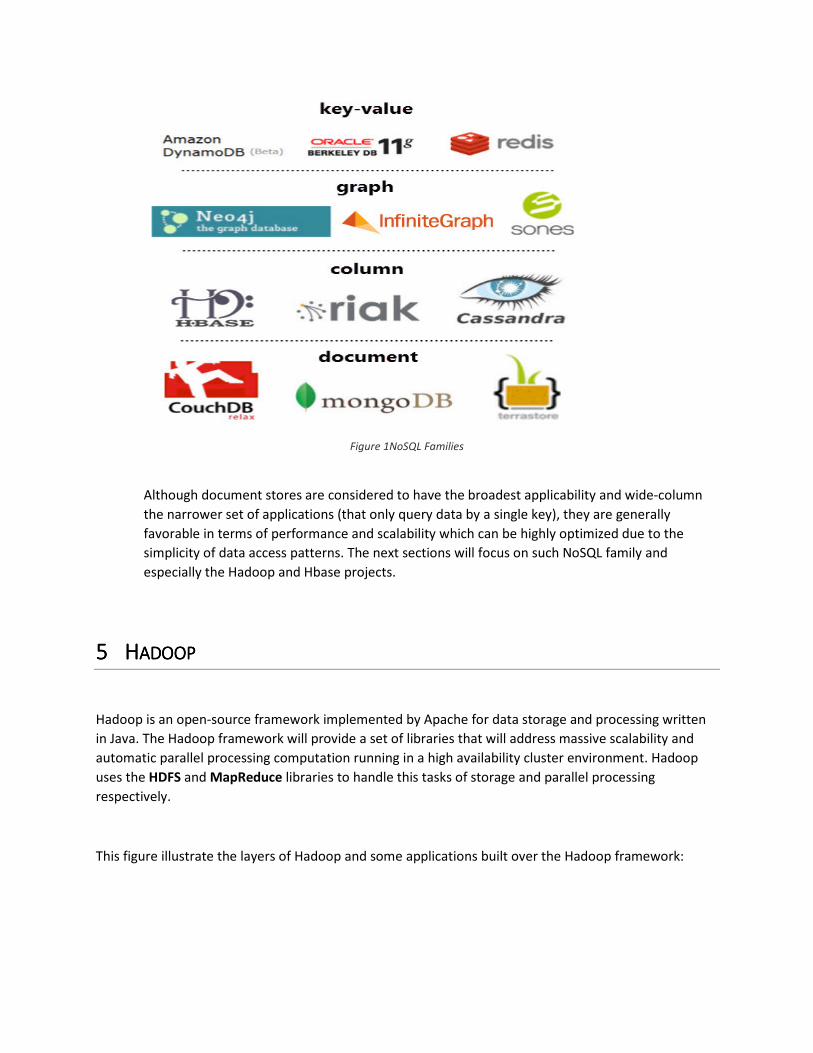
Figure 1NoSQL Families
Although document stores are considered to have the broadest applicability and wide-column
the narrower set of applications (that only query data by a single key), they are generally
favorable in terms of performance and scalability which can be highly optimized due to the
simplicity of data access patterns. The next sections will focus on such NoSQL family and
especially the Hadoop and Hbase projects.
5555 HHHHADOOPADOOPADOOPADOOP
Hadoop is an open-source framework implemented by Apache for data storage and processing written
in Java. The Hadoop framework will provide a set of libraries that will address massive scalability and
automatic parallel processing computation running in a high availability cluster environment. Hadoop
uses the HDFS and MapReduce libraries to handle this tasks of storage and parallel processing
respectively.
This figure illustrate the layers of Hadoop and some applications built over the Hadoop framework:
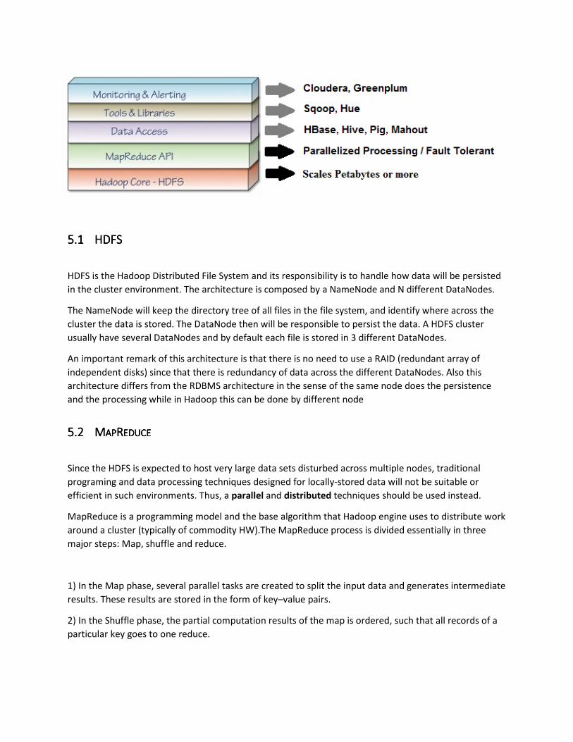
5.15.15.15.1 HDFSHDFSHDFSHDFS
HDFS is the Hadoop Distributed File System and its responsibility is to handle how data will be persisted
in the cluster environment. The architecture is composed by a NameNode and N different DataNodes.
The NameNode will keep the directory tree of all files in the file system, and identify where across the
cluster the data is stored. The DataNode then will be responsible to persist the data. A HDFS cluster
usually have several DataNodes and by default each file is stored in 3 different DataNodes.
An important remark of this architecture is that there is no need to use a RAID (redundant array of
independent disks) since that there is redundancy of data across the different DataNodes. Also this
architecture differs from the RDBMS architecture in the sense of the same node does the persistence
and the processing while in Hadoop this can be done by different node
5.25.25.25.2 MMMMAPAPAPAPRRRREDUCEEDUCEEDUCEEDUCE
Since the HDFS is expected to host very large data sets disturbed across multiple nodes, traditional
programing and data processing techniques designed for locally-stored data will not be suitable or
efficient in such environments. Thus, a parallel and distributed techniques should be used instead.
MapReduce is a programming model and the base algorithm that Hadoop engine uses to distribute work
around a cluster (typically of commodity HW).The MapReduce process is divided essentially in three
major steps: Map, shuffle and reduce.
1) In the Map phase, several parallel tasks are created to split the input data and generates intermediate
results. These results are stored in the form of key–value pairs.
2) In the Shuffle phase, the partial computation results of the map is ordered, such that all records of a
particular key goes to one reduce.
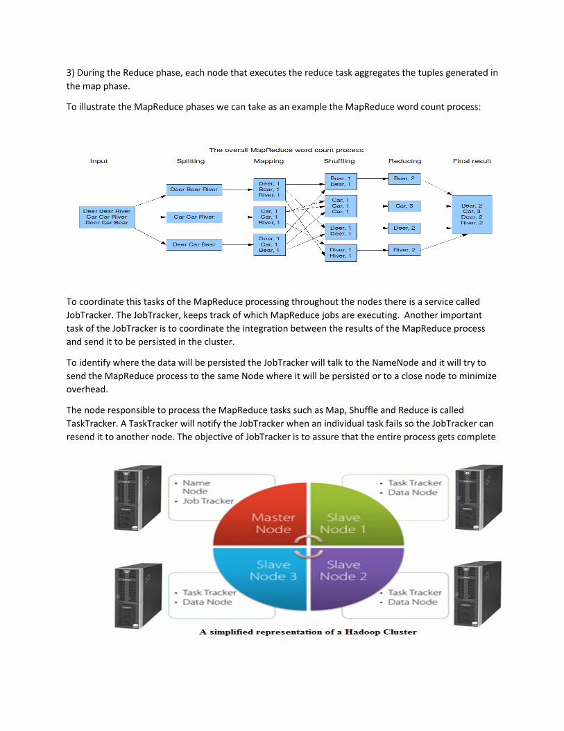
3) During the Reduce phase, each node that executes the reduce task aggregates the tuples generated in
the map phase.
To illustrate the MapReduce phases we can take as an example the MapReduce word count process:
To coordinate this tasks of the MapReduce processing throughout the nodes there is a service called
JobTracker. The JobTracker, keeps track of which MapReduce jobs are executing. Another important
task of the JobTracker is to coordinate the integration between the results of the MapReduce process
and send it to be persisted in the cluster.
To identify where the data will be persisted the JobTracker will talk to the NameNode and it will try to
send the MapReduce process to the same Node where it will be persisted or to a close node to minimize
overhead.
The node responsible to process the MapReduce tasks such as Map, Shuffle and Reduce is called
TaskTracker. A TaskTracker will notify the JobTracker when an individual task fails so the JobTracker can
resend it to another node. The objective of JobTracker is to assure that the entire process gets complete
5.35.35.35.3 YARNYARNYARNYARN –––– HHHHADOOPADOOPADOOPADOOP NNNNEXT EXT EXT EXT GGGGENERATION ENERATION ENERATION ENERATION MMMMAPAPAPAPRRRREDUCE EDUCE EDUCE EDUCE
Yarn is an improvement of the MapReduce process described earlier. The fundamental idea is to split up
the two major functionalities of the JobTracker, resource management and job scheduling/monitoring,
into separate services. This new architecture will bring more flexibility and even more scalability to
Hadoop architecture.
Yarn is example that the technology keeps evolving since its creation about 10 years ago. The Hadoop
growth has been exponential and currently the major technology players uses Hadoop. One example, is
the Windows Azure a solution for cloud computing built with Hadoop created by Microsoft.
6666 HHHHBASEBASEBASEBASE
6.16.16.16.1 AAAABOUT BOUT BOUT BOUT HHHHBASEBASEBASEBASE
HBase is a wide-column NoSQL DBMS as explained in earlier versions. Hbase is part of the Hadoop
ecosystem and is an overlay running on top of Hadoop HDFS. It is well suited for sparse data sets, which
are common in many big data use cases. Hbase was based on Google BigTable model and shares its
features.
6.1.16.1.16.1.16.1.1 FolloFolloFolloFollowing the wing the wing the wing the Big Table ModelBig Table ModelBig Table ModelBig Table Model
BigTable is a large map that is indexed by a row key, column key, and a timestamp. Each value within the
map is an array of bytes that is interpreted by the application. Every read or write of data to a row is
atomic, regardless of how many different columns are read or written within that row.
Some basic features of BigTable:
6.1.1.16.1.1.16.1.1.16.1.1.1 Map Map Map Map
A map is an associative array allowing a quick value look up to a corresponding key. Bigtable is a
collection of (key, value) pairs where the key identifies a row and the value is the set of columns.
6.1.1.26.1.1.26.1.1.26.1.1.2 Sparse Sparse Sparse Sparse
The table is sparse, meaning that different rows in a table may use different columns, with many of the
columns empty for a particular row.
6.1.1.36.1.1.36.1.1.36.1.1.3 Sorted Sorted Sorted Sorted
Most associative arrays are not sorted. A key is hashed to a position in a table. Bigtable sorts its data by
keys. This helps keep related data close together, usually on the same machine — assuming that one
structures keys in such a way that sorting brings the data together. For example, if domain names are
used as keys in a Bigtable, it makes sense to store them in reverse order to ensure that related domains
are close together. For example: be.ac.ulb.code be.ac.ulb.cs be.ac.ulb.www
6.1.1.46.1.1.46.1.1.46.1.1.4 Multidimensional Multidimensional Multidimensional Multidimensional
A table is indexed by rows. Each row contains one or more named column families. Column families are
defined when the table is first created. Within a column family, one may have one or more named
columns. All data within a column family is usually of the same type. The implementation of Bigtable
usually compresses all the columns within a column family together. Columns within a column family
can be created on the fly. Rows, column families and columns provide a three-level naming hierarchy in
identifying data.
6.1.1.56.1.1.56.1.1.56.1.1.5 TimeTimeTimeTime----based based based based
Time is another dimension in Bigtable data. Every column family may keep multiple versions of column
family data. If an application does not specify a timestamp, it will retrieve the latest version of the
column family. Alternatively, it can specify a timestamp and get the latest version that is earlier than or
equal to that timestamp.
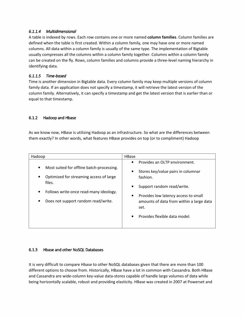
6.1.26.1.26.1.26.1.2 Hadoop andHadoop andHadoop andHadoop and HbaseHbaseHbaseHbase
As we know now, HBase is utilizing Hadoop as an infrastructure. So what are the differences between
them exactly? In other words, what features HBase provides on top (or to compliment) Hadoop
Hadoop HBase
• Most suited for offline batch-processing.
• Optimized for streaming access of large
files.
• Follows write-once read-many ideology.
• Does not support random read/write.
• Provides an OLTP environment.
• Stores key/value pairs in columnar
fashion.
• Support random read/write.
• Provides low latency access to small
amounts of data from within a large data
set.
• Provides flexible data model.
6.1.36.1.36.1.36.1.3 Hbase and otherHbase and otherHbase and otherHbase and other NoSQL DatabasesNoSQL DatabasesNoSQL DatabasesNoSQL Databases
It is very difficult to compare Hbase to other NoSQL databases given that there are more than 100
different options to choose from. Historically, HBase have a lot in common with Cassandra. Both HBase
and Cassandra are wide-column key-value data-stores capable of handle large volumes of data while
being horizontally scalable, robust and providing elasticity. HBase was created in 2007 at Powerset and
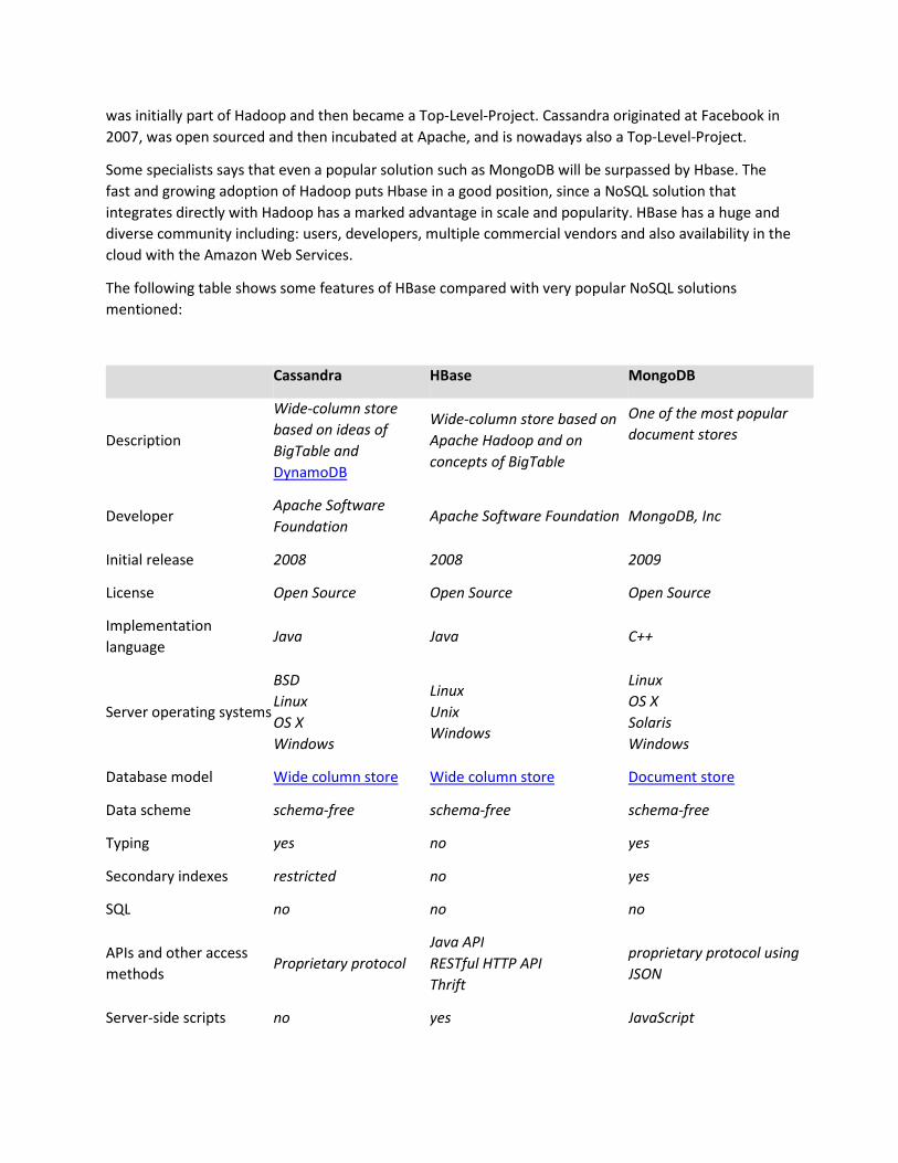
was initially part of Hadoop and then became a Top-Level-Project. Cassandra originated at Facebook in
2007, was open sourced and then incubated at Apache, and is nowadays also a Top-Level-Project.
Some specialists says that even a popular solution such as MongoDB will be surpassed by Hbase. The
fast and growing adoption of Hadoop puts Hbase in a good position, since a NoSQL solution that
integrates directly with Hadoop has a marked advantage in scale and popularity. HBase has a huge and
diverse community including: users, developers, multiple commercial vendors and also availability in the
cloud with the Amazon Web Services.
The following table shows some features of HBase compared with very popular NoSQL solutions
mentioned:
Cassandra HBase MongoDB
Description
Wide-column store
based on ideas of
BigTable and
DynamoDB
Wide-column store based on
Apache Hadoop and on
concepts of BigTable
One of the most popular
document stores
Developer Apache Software
Foundation Apache Software Foundation MongoDB, Inc
Initial release 2008 2008 2009
License Open Source Open Source Open Source
Implementation
language Java Java C++
Server operating systems
BSD
Linux
OS X
Windows
Linux
Unix
Windows
Linux
OS X
Solaris
Windows
Database model Wide column store Wide column store Document store
Data scheme schema-free schema-free schema-free
Typing yes no yes
Secondary indexes restricted no yes
SQL no no no
APIs and other access
methods Proprietary protocol
Java API
RESTful HTTP API
Thrift
proprietary protocol using
JSON
Server-side scripts no yes JavaScript
Triggers no yes no
Partitioning methods Sharding Sharding Sharding
Replication methods selectable replication
factor selectable replication factor Master-slave replication
MapReduce yes yes yes
Consistency concepts Eventual Consistency
Immediate Consistency Immediate Consistency
Eventual Consistency
Immediate Consistency
Foreign keys no no no
Transaction concepts no no no
Concurrency yes yes yes
Durability yes yes yes
User concepts
Access rights for users
can be defined per
object
Access Control Lists (ACL)
Users can be defined with
full access or read-only
access
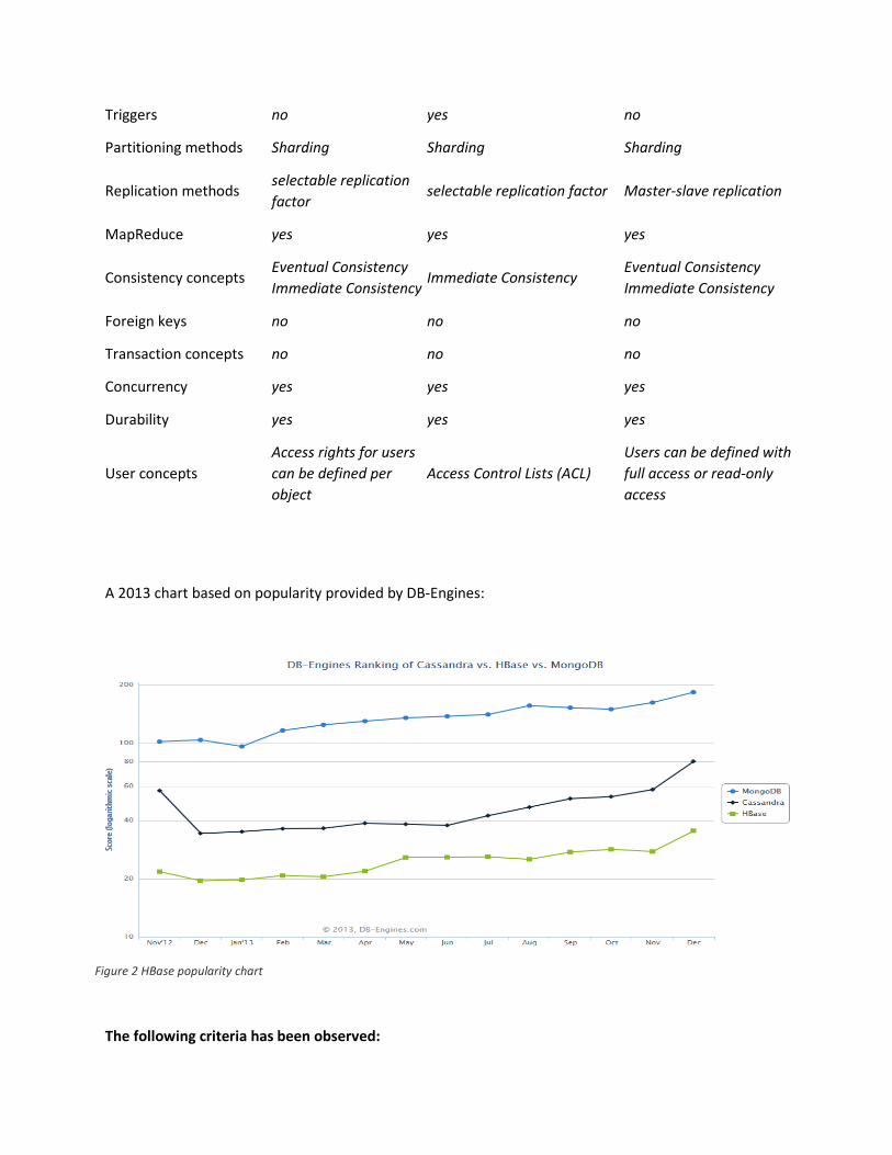
A 2013 chart based on popularity provided by DB-Engines:
The following criteria has been observed:
Figure 2 HBase popularity chart
• Number of mentions of the system on websites
• General interest in the system
• Frequency of technical discussions about the system
• Number of job offers, in which the system is mentioned
6.26.26.26.2 HHHHBASE UNDER BASE UNDER BASE UNDER BASE UNDER THE HOODTHE HOODTHE HOODTHE HOOD
6.2.16.2.16.2.16.2.1 BottomBottomBottomBottom----up architectureup architectureup architectureup architecture
6.2.1.16.2.1.16.2.1.16.2.1.1 Logical Table OrganizationLogical Table OrganizationLogical Table OrganizationLogical Table Organization
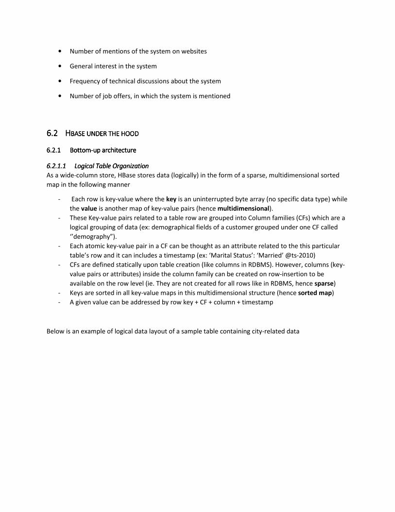
As a wide-column store, HBase stores data (logically) in the form of a sparse, multidimensional sorted
map in the following manner
- Each row is key-value where the key is an uninterrupted byte array (no specific data type) while
the value is another map of key-value pairs (hence multidimensional).
- These Key-value pairs related to a table row are grouped into Column families (CFs) which are a
logical grouping of data (ex: demographical fields of a customer grouped under one CF called
‘’demography”).
- Each atomic key-value pair in a CF can be thought as an attribute related to the this particular
table’s row and it can includes a timestamp (ex: ‘Marital Status’: ‘Married’ @ts-2010)
- CFs are defined statically upon table creation (like columns in RDBMS). However, columns (key-
value pairs or attributes) inside the column family can be created on row-insertion to be
available on the row level (ie. They are not created for all rows like in RDBMS, hence sparse)
- Keys are sorted in all key-value maps in this multidimensional structure (hence sorted map)
- A given value can be addressed by row key + CF + column + timestamp
Below is an example of logical data layout of a sample table containing city-related data
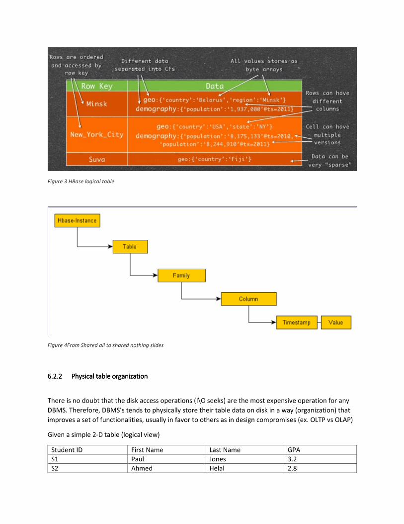
Figure 3 HBase logical table
Figure 4From Shared all to shared nothing slides
6.2.26.2.26.2.26.2.2 Physical table organizationPhysical table organizationPhysical table organizationPhysical table organization
There is no doubt that the disk access operations (I\O seeks) are the most expensive operation for any
DBMS. Therefore, DBMS’s tends to physically store their table data on disk in a way (organization) that
improves a set of functionalities, usually in favor to others as in design compromises (ex. OLTP vs OLAP)
Given a simple 2-D table (logical view)
Student ID First Name Last Name GPA
S1 Paul Jones 3.2
S2 Ahmed Helal 2.8
S3 Peter Smith 3.2
S4 Mark Jones 3.8
A row-oriented DBMS will serialize each row to the disk as follows
001: s1,Paul,Jones,3.2 ; 002:s2,Ahmed,Helal,2.8; s3:300,Peter ..etc
These kind of systems are designed to work best when entire row operations are more frequent (ex.
Insert, delete and retrieve row\s). This matches the common use-case of retrieving the information
about a particular object. However, these DBMS’s are not designed to work on entire data sets,
especially large ones that can’t fit entirely in memory, as opposed to specific rows. Although this kind of
column-oriented operations can be enhanced by using indexes, maintaining indexes adds overhead to
the system especially when adding new data to the table.
On the other hand, a column-oriented DBMS (like HBase) will serialize all the values of a column
together as follows
S1:001, s2:002, s3:003, s4:004 ; Paul:001, Ahmed:002, Peter:003, Mark:004 ; ..etc
This organization can seem similar with how a RDBMS handle indexes. However, the mapping of the
data is different. For example the ‘last name’ column can be serialized in this way since it contains
duplicates
Jones:001, 004, Helal:002, Smith:003
In this general column-oriented layout aggregation over many rows but smaller subset of columns can
be quite efficient as well as optimized compression for storage.
That was a general intro on how column-oriented databases physically stores data compared to row-
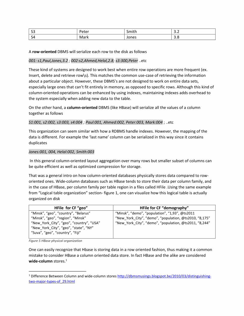
oriented ones. Wide-column databases such as HBase tends to store their data per column family, and
in the case of HBase, per column family per table region in a files called HFile .Using the same example
from “Logical table organization” section- figure 1, one can visualize how this logical table is actually
organized on disk
HFile for CF “geo” HFile for CF “demography”
“Minsk”, “geo”, “country”, “Belarus”
“Minsk”, “geo”, “region”, “Minsk”
“New_York_City”, “geo”, “country”, “USA”
“New_York_City”, “geo”, “state”, “NY”
“Suva”, “geo”, “country”, “Fiji”
“Minsk”, “demo”, “population”, “1,93”, @ts2011
“New_York_City”, “demo”, “population, @ts2010, “8,175”
“New_York_City”, “demo”, “population, @ts2011, “8,244”
Figure 5 HBase physical organization
One can easily recognize that Hbase is storing data in a row oriented fashion, thus making it a common
mistake to consider HBase a column oriented data store. In fact HBase and the alike are considered
wide-column stores.1
1 Difference Between Column and wide-column stores http://dbmsmusings.blogspot.be/2010/03/distinguishing-
two-major-types-of_29.html
6.2.36.2.36.2.36.2.3 Table ShardingTable ShardingTable ShardingTable Sharding
Sharding is the term used to describe the technique HBase use to distribute table data amongst nodes in
the cluster to achieve scalability. Table sharding works in simple steps as follows
- Tables are horizontally partitioned into ‘Regions’ which are the atoms of distribution
- Regions are defined by start and end row keys
- Regions are assigned to HRegionServer’s, the assignment is done by the HMaster server (HBase
servers will be explained in the next section)
- Regions are distributed evenly across RegionServers, A region is assigned to only one
HRegionServer
- A region can split as it grows, Thus dynamically adjusting to the dataset
6.2.46.2.46.2.46.2.4 HBase nodesHBase nodesHBase nodesHBase nodes topologytopologytopologytopology
Since HBase is utilizing Hadoop for its distributed data storage and cluster management, it follows
somehow a similar master\slave architecture. A typical HBase with Hadoop setup will contain the
following servers (in this context the term ‘server’ is used to describe a process and not a machine)
- HMaster: the master node of the HBase grid that coordinates the cluster and responsible for
administrative operations such as regions assignment.
- HRegionServer: slave nodes that hosts table ‘regions’, mainly buffering I/O operations and log
management, permanent data storage is done on HDFS data nodes as will be explained soon
HBase utilize Apache ZooKeeper which is a client/server system for distributed coordination that
exposes an interface similar to a file system, where each node (called a znode) has a name and can be
identified using a file system-like path (for example, /root-znode/sub-znode/my-znode).
In HBase, ZooKeeper coordinates, communicates, and shares state between the Masters and Region
Servers. HBase has a design policy of using ZooKeeper only for transient data (that is, for coordination
and state communication). Thus if the HBase’s ZooKeeper data is removed, only the transient operations
are affected – data can continue to be written and read to/from HBase.
6.2.56.2.56.2.56.2.5 Integrated OverviewIntegrated OverviewIntegrated OverviewIntegrated Overview
Gluing the 3 components’ (HBase, Hadoop and ZooKeeper) services one might conclude the below
integrated architecture
Figure 6 Integrated overview
Usually the Hadoop NameNode and HMaster will be running on the same box (node) while each
HRegionServer and Hadoop DataNode will be coupled together. The same goes for MapReduce roles as
illustrated in the diagram.
It’s worth mentioning that both the HMaster and HRegionServers are fairly stateless and machine
independent since the permanent data storage is applied on the HDFS DataNode. To illustrate the
connection between different services, the following steps will explain how a write request is typically
handled
- A HRegionServer receives a write request, it first writes changes in memory commit log
- At some point it the HRegionServer decides it’s time to write changes permanently into HDFS
- Since a HRegionServer and a HDFS DataNode are usually running on the same machine, the
HDFS creates 3 replicas of the data file (Hadoop strategy for high availability) and stores them
on the local machine and 2 other DataNodes. Thus, in most cases the HRegionServer will always
have a local copy of the regions it is serving (data locality)
Handling Handling Handling Handling failoverfailoverfailoverfailover
Based on the above architecture, when a DataNode fails, it is handled by HDFS replication. When a
HRegionServer fails, the HMaster handles it automatically by re-assigning regions to available region
servers. And finally, if the HMaster fails, it can be replaced by secondary master. (However, the single-
point of failure regarding HMaster is highly argued and the next release of HBase is expected to solve
this problem completely)
6.2.66.2.66.2.66.2.6 Client app: which node to communicate with?Client app: which node to communicate with?Client app: which node to communicate with?Client app: which node to communicate with?
It can be wrongly assumed that since HBase is applying a Master/Slave architecture, it is then handling
all incoming requests from client apps by the HMaster, eventually causing a bottleneck. However, this is
not the case with HBase. As mentioned before the HMaster is responsible only for managing the cluster
and administrative tasks.
To read or write rows, clients don’t have to go through the HMaster, they can directly contact the region
server containing the specified row or the set of region servers responsible for handling a set of keys. To
do so, clients’ needs to query a system table called the ‘META’ table.
‘Meta’ is a system table that keeps track if regions assignments, which is the start and end keys of a
table (region) assigned to a region servers. And since it is a table like the others, the client needs to
know on which node it is residing. The location of the META table is stored on a ZooKeeper node
assigned by the HMaster, so clients reads directly the ZooKeeper Node to get the address of the region
server containing the META table.
6.2.76.2.76.2.76.2.7 Data pathData pathData pathData path
This section will illustrate the logical sequence of operations and components involved to execute both
read and write information. Before going into the steps the below figure illustrates the hierarchy of
HBase objects
Figure 7 HBase data objects hierarchy
In the above model, MemStore is the memory buffer that holds in-memory modifications to the store
before flushing it to a StoreFile. A StoreFile is the physical file used to holds the data and a Store may
contain multiple store files (created by each MemStore Flush) that can be merged together by the
system in a process called “compaction”
6.2.7.16.2.7.16.2.7.16.2.7.1 Write PatWrite PatWrite PatWrite Pathhhh
- The client issues a put command in the format of (row-key, Column Family, column, <<value>>)
- The client asks ZooKeeper the location of the META table
- The client scans it to find the region server responsible for the new key
- The client ask the region server insert\update\delete the specified key-value
- The region server process the request by dispatching it the region responsible for the key (a
region server may contain multiple regions), by turn to the corresponding Store based on the
column family
o The store writes the operation to a write-ahead-log (to insure durability)
o The key-value is added to the store MemStore (to be sorted)
o Once the MemStore reaches a specific size it is flushed to a store file
o When a MemStore flushs its content, a process called ‘minor compaction’ is triggered
that will merge some store files together (based on an algorithm that is out-of-scope of
this report)
6.2.7.26.2.7.26.2.7.26.2.7.2 Read PathRead PathRead PathRead Path
- The client issues a get command in the format by identifying the required key.
- The client asks ZooKeeper the location of the META table
- The client scans it to find the region server responsible for the required key
- The client asks the region server to get the specified key\value
- Region server dispatches the request to the region responsible for the key
o Both MemStore and store files are scanned for the key
o Since multiple store files can be found (ex. For insert & deletes), they need to be all
scanned applying some optimizations like filtering by start\end key or having a bloom
filter on each file (a bloom filter is a data structure designed to tell rapidly and memory-
efficiently, whether an element is present in a set or not)
6.2.86.2.86.2.86.2.8 Data model operationsData model operationsData model operationsData model operations
In this section we will demonstrate a use case on HBase while illustrating some modeling aspects, using
the HBase shell for simple operations and HBase Java API for data generation and map-reduce.
6.2.8.16.2.8.16.2.8.16.2.8.1 Insights modelInsights modelInsights modelInsights model
A common use case that is being used in HBase is the “Web Insights” data model. Given a video sharing
website (like Youtube), we need to track multiple metrics for each videos (number of views, unique
views, likes, comments, locations ..etc) on different granularity (as it happen, Daily aggregates, Monthly
aggregates, Totals). For simplicity we will use one metric “number of views” and we will assume that
each minute the website is logging the number of views it received for a given video (if it has been
viewed only).
To model this in HBase, we can create a single table called “Insights” were each row represents a single
video, with 2 column families “MinutesCounters” and “DailyCounters”. In the minutes-counters CF we
can store the website logging information by dynamically creating columns representing a date-time
value (on a minute grain) along with a values that represents the “NumberOfViews” (for that video at
this minute). On the other hand, we can run a map-reduce code to aggregate the values in the
“MinutesCounters” column family and insert it in the “DailyCounters” for each video.
Figure 8 Insights Mode
Time-to-live
In this highly scalable database we can optimize the storage by setting a Time-To-Live (TTL) flag on the
column family level indicating that HBase should delete the cells in this CF after “x” seconds. In our
model we will set the TTL on “MinutesCounters” CF to 7 days for demonstration purposes.
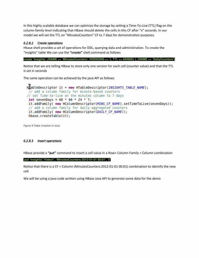
6.2.8.26.2.8.26.2.8.26.2.8.2 Create operationsCreate operationsCreate operationsCreate operations
Hbase shell provides a set of operations for DDL, querying data and administration. To create the
“Insights” table We can use the “create” shell command as follows
create ‘Insights′, {NAME => ‘MinutesCounters′, VERSIONS => 1, TTL => 604800} }, {NAME => ‘DailyCounters′}
Notice that we are telling HBase to store only one version for each cell (counter value) and that the TTL
is set in seconds
The same operation can be achieved by the java API as follows
Figure 9 Table Creation in Java
6.2.8.36.2.8.36.2.8.36.2.8.3 InsertInsertInsertInsert operationsoperationsoperationsoperations
HBase provide a “put” command to insert a cell value in a Row+ Column Family + Column combination
put ‘Insights′,’Video1’, ‘MinutesCounters:2012-01-01 00:01′, ‘5’
Notice that there is a CF + Column (MinutesCounters:2012-01-01 00:01) combination to identify the new
cell.
We will be using a java code written using HBase Java API to generate some data for the demo
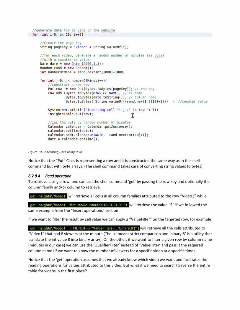
Figure 10 Generating Data using Java
Notice that the “Put” Class is representing a row and it is constructed the same way as in the shell
command but with byte arrays. (The shell command takes care of converting string values to bytes)
6.2.8.46.2.8.46.2.8.46.2.8.4 Read operationRead operationRead operationRead operation
To retrieve a single row, one can use the shell command ‘get’ by passing the row key and optionally the
column family and\or column to retrieve
get ‘Insights′,’Video1’ will retrieve all cells in all column families attributed to the row “Video1” while
get ‘Insights′,’Video1’, ‘MinutesCounters:2012-01-01 00:01′ will retrieve the value “5” if we followed the
same example from the “Insert operations” section
If we want to filter the result by cell value we can apply a “ValueFilter” on the targeted row, for example
get ‘Insights′,’Video1’, { FILTER => “ValueFilter( = , ‘binary:8’)” } will retrieve all the cells attributed to
“Video1” that had 8 viewers at the minute (The ‘=’ means strict comparison and ‘binary:8’ is a utility that
translate the int value 8 into binary array). On the other, if we want to filter a given row by column name
(minutes in our case) we can use the ‘QualifierFilter’ instead of ‘ValueFilter’ and pass it the required
column name (if we want to know the number of viewers for a specific video at a specific time)
Notice that the ‘get’ operation assumes that we already know which video we want and facilitates the
reading operations for values attributed to this video, But what if we need to search\traverse the entire
table for videos in the first place?
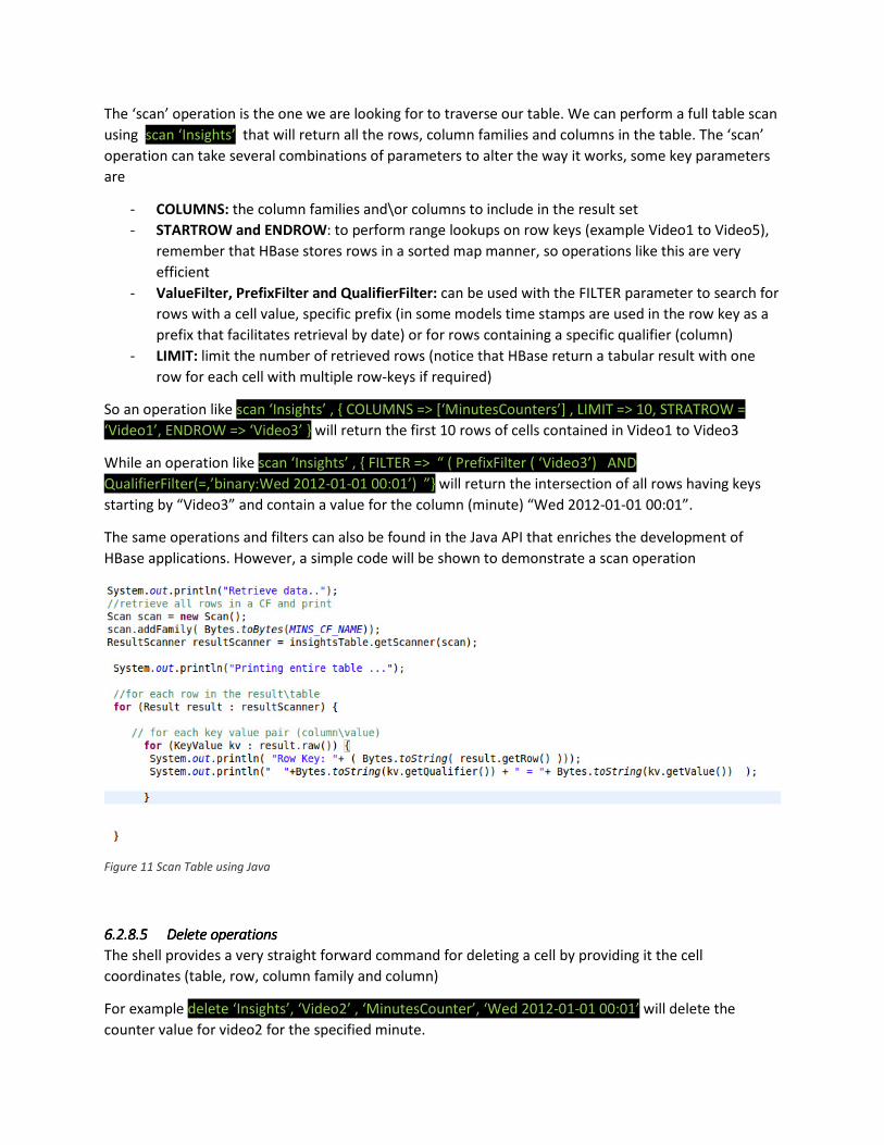
The ‘scan’ operation is the one we are looking for to traverse our table. We can perform a full table scan
using scan ‘Insights’ that will return all the rows, column families and columns in the table. The ‘scan’
operation can take several combinations of parameters to alter the way it works, some key parameters
are
- COLUMNS: the column families and\or columns to include in the result set
- STARTROW and ENDROW: to perform range lookups on row keys (example Video1 to Video5),
remember that HBase stores rows in a sorted map manner, so operations like this are very
efficient
- ValueFilter, PrefixFilter and QualifierFilter: can be used with the FILTER parameter to search for
rows with a cell value, specific prefix (in some models time stamps are used in the row key as a
prefix that facilitates retrieval by date) or for rows containing a specific qualifier (column)
- LIMIT: limit the number of retrieved rows (notice that HBase return a tabular result with one
row for each cell with multiple row-keys if required)
So an operation like scan ‘Insights’ , { COLUMNS => [‘MinutesCounters’] , LIMIT => 10, STRATROW =
‘Video1’, ENDROW => ‘Video3’ } will return the first 10 rows of cells contained in Video1 to Video3
While an operation like scan ‘Insights’ , { FILTER => “ ( PrefixFilter ( ‘Video3’) AND
QualifierFilter(=,’binary:Wed 2012-01-01 00:01’) ”} will return the intersection of all rows having keys
starting by “Video3” and contain a value for the column (minute) “Wed 2012-01-01 00:01”.
The same operations and filters can also be found in the Java API that enriches the development of
HBase applications. However, a simple code will be shown to demonstrate a scan operation
Figure 11 Scan Table using Java
6.2.8.56.2.8.56.2.8.56.2.8.5 Delete operationsDelete operationsDelete operationsDelete operations
The shell provides a very straight forward command for deleting a cell by providing it the cell
coordinates (table, row, column family and column)
For example delete ‘Insights’, ‘Video2’ , ‘MinutesCounter’, ‘Wed 2012-01-01 00:01’ will delete the
counter value for video2 for the specified minute.
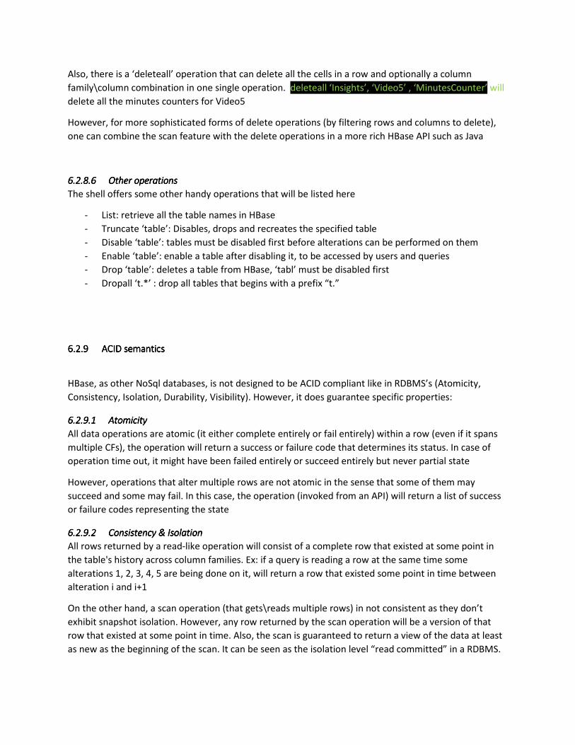
Also, there is a ‘deleteall’ operation that can delete all the cells in a row and optionally a column
family\column combination in one single operation. deleteall ‘Insights’, ‘Video5’ , ‘MinutesCounter’ will
delete all the minutes counters for Video5
However, for more sophisticated forms of delete operations (by filtering rows and columns to delete),
one can combine the scan feature with the delete operations in a more rich HBase API such as Java
6.2.8.66.2.8.66.2.8.66.2.8.6 Other operations Other operations Other operations Other operations
The shell offers some other handy operations that will be listed here
- List: retrieve all the table names in HBase
- Truncate ‘table’: Disables, drops and recreates the specified table
- Disable ‘table’: tables must be disabled first before alterations can be performed on them
- Enable ‘table’: enable a table after disabling it, to be accessed by users and queries
- Drop ‘table’: deletes a table from HBase, ‘tabl’ must be disabled first
- Dropall ‘t.*’ : drop all tables that begins with a prefix “t.”
6.2.96.2.96.2.96.2.9 ACIDACIDACIDACID semantics semantics semantics semantics
HBase, as other NoSql databases, is not designed to be ACID compliant like in RDBMS’s (Atomicity,
Consistency, Isolation, Durability, Visibility). However, it does guarantee specific properties:
6.2.9.16.2.9.16.2.9.16.2.9.1 AtomicityAtomicityAtomicityAtomicity
All data operations are atomic (it either complete entirely or fail entirely) within a row (even if it spans
multiple CFs), the operation will return a success or failure code that determines its status. In case of
operation time out, it might have been failed entirely or succeed entirely but never partial state
However, operations that alter multiple rows are not atomic in the sense that some of them may
succeed and some may fail. In this case, the operation (invoked from an API) will return a list of success
or failure codes representing the state
6.2.9.26.2.9.26.2.9.26.2.9.2 Consistency & IsolationConsistency & IsolationConsistency & IsolationConsistency & Isolation
All rows returned by a read-like operation will consist of a complete row that existed at some point in
the table's history across column families. Ex: if a query is reading a row at the same time some
alterations 1, 2, 3, 4, 5 are being done on it, will return a row that existed some point in time between
alteration i and i+1
On the other hand, a scan operation (that gets\reads multiple rows) in not consistent as they don’t
exhibit snapshot isolation. However, any row returned by the scan operation will be a version of that
row that existed at some point in time. Also, the scan is guaranteed to return a view of the data at least
as new as the beginning of the scan. It can be seen as the isolation level “read committed” in a RDBMS.
6.2.9.36.2.9.36.2.9.36.2.9.3 DurabilityDurabilityDurabilityDurability
Any success code returned by an altar-operation implies that the altered version is visible to both the
client who performed the operation and any other client with whom it later communicates through side
channels, that is any version of a cell that has been returned to read operation is guaranteed to be
durably stored.
Also, one can guarantee the following
- All visible data is also durable data (a read will never return data that has not been durable on
disk)
- Operations that returned success code are made durable on disk
- Operations that returned failure code will not be made durable
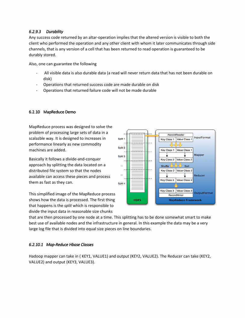
6.2.106.2.106.2.106.2.10 MapReduceMapReduceMapReduceMapReduce DemoDemoDemoDemo
MapReduce process was designed to solve the
problem of processing large sets of data in a
scalazble way. It is designed to increases in
performance linearly as new commodity
machines are added.
Basically it follows a divide-and-conquer
approach by splitting the data located on a
distributed file system so that the nodes
available can access these pieces and process
them as fast as they can.
This simplified image of the MapReduce process
shows how the data is processed. The first thing
that happens is the split which is responsible to
divide the input data in reasonable size chunks
that are then processed by one node at a time. This splitting has to be done somewhat smart to make
best use of available nodes and the infrastructure in general. In this example the data may be a very
large log file that is divided into equal size pieces on line boundaries.
6.2.10.16.2.10.16.2.10.16.2.10.1 MapMapMapMap----Reduce Hbase ClassesReduce Hbase ClassesReduce Hbase ClassesReduce Hbase Classes
Hadoop mapper can take in ( KEY1, VALUE1) and output (KEY2, VALUE2). The Reducer can take (KEY2,
VALUE2) and output (KEY3, VALUE3).
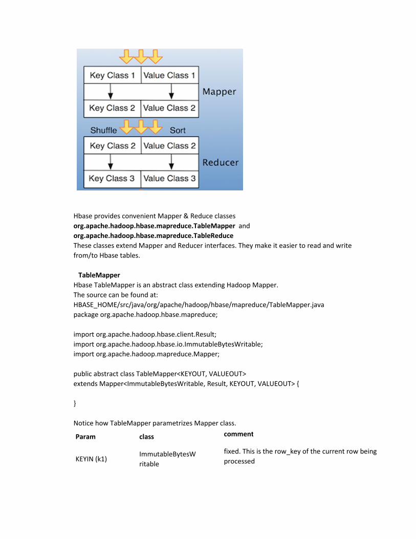
Hbase provides convenient Mapper & Reduce classes
org.apache.hadoop.hbase.mapreduce.TableMapper and
org.apache.hadoop.hbase.mapreduce.TableReduce
These classes extend Mapper and Reducer interfaces. They make it easier to read and write
from/to Hbase tables.
TableMapper
Hbase TableMapper is an abstract class extending Hadoop Mapper.
The source can be found at:
HBASE_HOME/src/java/org/apache/hadoop/hbase/mapreduce/TableMapper.java
package org.apache.hadoop.hbase.mapreduce;
import org.apache.hadoop.hbase.client.Result;
import org.apache.hadoop.hbase.io.ImmutableBytesWritable;
import org.apache.hadoop.mapreduce.Mapper;
public abstract class TableMapper<KEYOUT, VALUEOUT>
extends Mapper<ImmutableBytesWritable, Result, KEYOUT, VALUEOUT> {
}
Notice how TableMapper parametrizes Mapper class.
Param class comment
KEYIN (k1) ImmutableBytesW
ritable
fixed. This is the row_key of the current row being
processed
VALUEIN
(v1) Result fixed. This is the value (result) of the row
KEYOUT
(k2) user specified customizable
VALUEOUT
(v2) user specified customizable
The input key/value for TableMapper is fixed. We are free to customize output key/value
classes. This is a noticeable difference compared to writing a straight hadoop mapper.
TableReducer
src : HBASE_HOME/src/java/org/apache/hadoop/hbase/mapreduce/TableReducer.java
package org.apache.hadoop.hbase.mapreduce;
import org.apache.hadoop.io.Writable;
import org.apache.hadoop.mapreduce.Reducer;
public abstract class TableReducer<KEYIN, VALUEIN, KEYOUT>
extends Reducer<KEYIN, VALUEIN, KEYOUT, Writable> {
}
Let’ss look at the parameters:
Param Class
KEYIN (k2 - same as mapper
keyout) user-specified (same class as K2 ouput from mapper)
VALUEIN(v2 - same as mapper
valueout) user-specified (same class as V2 ouput from mapper)
KEYIN (k3) user-specified
VALUEOUT (k4) must be Writable
TableReducer can take any KEY2 / VALUE2 class and emit any KEY3 class, and a Writable VALUE4
class.
6.2.10.26.2.10.26.2.10.26.2.10.2 When should we applyWhen should we applyWhen should we applyWhen should we apply Map or ReduceMap or ReduceMap or ReduceMap or Reduce
If you want to import a large set of data into a HBase table you can read the data using a
Mapper and after aggregating it on a per key basis using a Reducer and finally writing it into a
HBase table. This involves the whole MapReduce stack including the shuffle and sort using
intermediate files. But what if you know that the data for example has a unique key? Why go
through the extra step of copying and sorting when there is always just exactly one key/value
pair? In this case would certainly be better to skip the reduce stage.
Same or different Tables
This is the an important distinction. The bottom line is, when you read a table in the Map stage
you should consider not writing back to that very same table in the same process. It could on
one hand hinder the proper distribution of regions across the nodes (open scanners block
regions splits) and on the other hand you may or may not see the new data as you scan. But
when you read from one table and write to another then you can do that in a single stage. So for
two different tables you can write your table updates directly in the TableMapper.map() while
with the same table you must write the same code in the TableReduce.reduce(). The reason is
that the Map stage completely reads a table and then passes the data on in intermediate files to
the Reduce stage. In turn this means that the Reducer reads from the distributed file system
(DFS) and writes into the now idle HBase table.
All of the above are simply recommendations based on what is currently available with HBase.
There is of course no reason not to scan and modify a table in the same process. But to avoid
certain non-deterministic issue it is in general not recommend. This also could be taken into
consideration when designing your HBase tables.
Key Distribution
Another specific requirement for an effective import is to have a random keys as they are read.
While this will be difficult if you scan a table in the Map phase, as keys are sorted, we may be
able to make use of this when reading from a raw data file. Instead of leaving the key the offset
of the file, as created by the TextOutputFormat for example, we could simply replace the rather
useless offset with a random key.
This will guarantee that the data is spread across all nodes more evenly. Especially the
HRegionServers will be very thankful as they each host as set of regions and random keys makes
for a random load on these regions. Of course this depends on how the data is written to the
raw files or how the real row keys are computed, but still a very valuable thing to keep in mind.
6.2.10.36.2.10.36.2.10.36.2.10.3 MapReduce Demo: Video Views counterMapReduce Demo: Video Views counterMapReduce Demo: Video Views counterMapReduce Demo: Video Views counter
For this example lets assume our Hbase has records of accessed video_logs. We record each
video that was accessed in a specific day. To simplify we are only logging the video_id and the
day of it was accessed. We can imagine all sorts of stats can be gathered, such as ip_address,
referred page, etc.
The schema looks like this:
video_timestamp => {
details => {
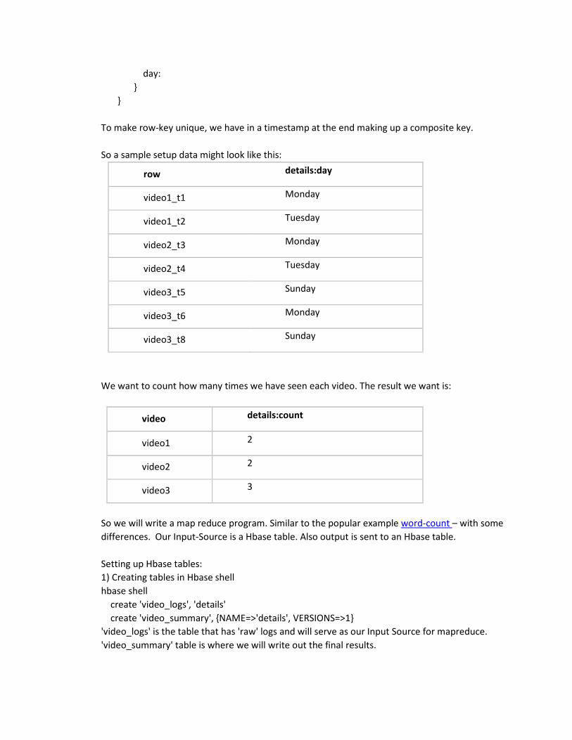
day:
}
}
To make row-key unique, we have in a timestamp at the end making up a composite key.
So a sample setup data might look like this:
row details:day
video1_t1 Monday
video1_t2 Tuesday
video2_t3 Monday
video2_t4 Tuesday
video3_t5 Sunday
video3_t6 Monday
video3_t8 Sunday
We want to count how many times we have seen each video. The result we want is:
video details:count
video1 2
video2 2
video3 3
So we will write a map reduce program. Similar to the popular example word-count – with some
differences. Our Input-Source is a Hbase table. Also output is sent to an Hbase table.
Setting up Hbase tables:
1) Creating tables in Hbase shell
hbase shell
create 'video_logs', 'details'
create 'video_summary', {NAME=>'details', VERSIONS=>1}
'video_logs' is the table that has 'raw' logs and will serve as our Input Source for mapreduce.
'video_summary' table is where we will write out the final results.
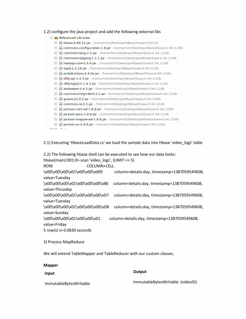
1.2) configure the java project and add the following external libs
2.1) Executing 'HbaseLoadData.cs' we load the sample data into Hbase 'video_logs' table
2.2) The following hbase shell can be executed to see how our data looks:
hbase(main):001:0> scan 'video_logs', {LIMIT => 5}
ROW COLUMN+CELL
\x00\x00\x00\x01\x00\x00\x009 column=details:day, timestamp=1387059549608,
value=Tuesday
\x00\x00\x00\x01\x00\x00\x00\x86 column=details:day, timestamp=1387059549608,
value=Thrusday
\x00\x00\x00\x01\x00\x00\x00\xD7 column=details:day, timestamp=1387059549608,
value=Tuesday
\x00\x00\x00\x01\x00\x00\x00\xDB column=details:day, timestamp=1387059549608,
value=Sunday
\x00\x00\x00\x01\x00\x00\x01. column=details:day, timestamp=1387059549608,
value=Friday
5 row(s) in 0.0830 seconds
3) Process MapReduce
We will extend TableMapper and TableReducer with our custom classes.
Mapper
Input Output
ImmutableBytesWritable ImmutableBytesWritable (videoID)
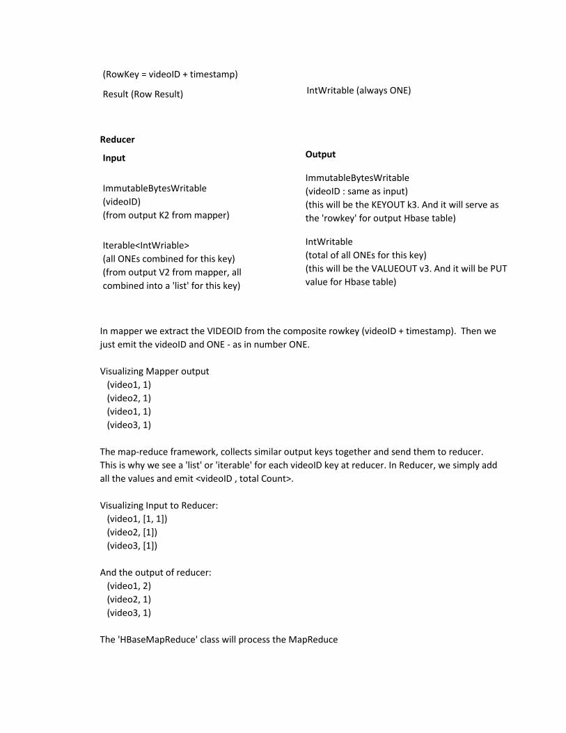
(RowKey = videoID + timestamp)
Result (Row Result) IntWritable (always ONE)
Reducer
Input Output
ImmutableBytesWritable
(videoID)
(from output K2 from mapper)
ImmutableBytesWritable
(videoID : same as input)
(this will be the KEYOUT k3. And it will serve as
the 'rowkey' for output Hbase table)
Iterable<IntWriable>
(all ONEs combined for this key)
(from output V2 from mapper, all
combined into a 'list' for this key)
IntWritable
(total of all ONEs for this key)
(this will be the VALUEOUT v3. And it will be PUT
value for Hbase table)
In mapper we extract the VIDEOID from the composite rowkey (videoID + timestamp). Then we
just emit the videoID and ONE - as in number ONE.
Visualizing Mapper output
(video1, 1)
(video2, 1)
(video1, 1)
(video3, 1)
The map-reduce framework, collects similar output keys together and send them to reducer.
This is why we see a 'list' or 'iterable' for each videoID key at reducer. In Reducer, we simply add
all the values and emit <videoID , total Count>.
Visualizing Input to Reducer:
(video1, [1, 1])
(video2, [1])
(video3, [1])
And the output of reducer:
(video1, 2)
(video2, 1)
(video3, 1)
The 'HBaseMapReduce' class will process the MapReduce
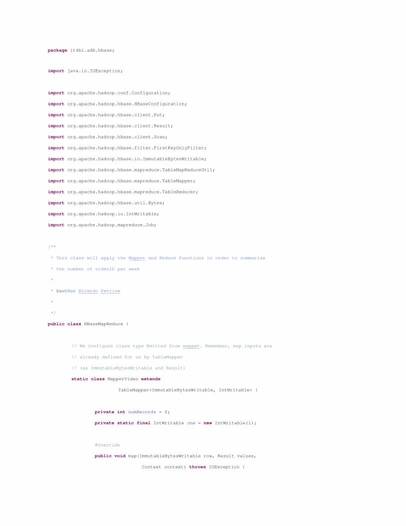
package it4bi.adb.hbase;
import java.io.IOException;
import org.apache.hadoop.conf.Configuration;
import org.apache.hadoop.hbase.HBaseConfiguration;
import org.apache.hadoop.hbase.client.Put;
import org.apache.hadoop.hbase.client.Result;
import org.apache.hadoop.hbase.client.Scan;
import org.apache.hadoop.hbase.filter.FirstKeyOnlyFilter;
import org.apache.hadoop.hbase.io.ImmutableBytesWritable;
import org.apache.hadoop.hbase.mapreduce.TableMapReduceUtil;
import org.apache.hadoop.hbase.mapreduce.TableMapper;
import org.apache.hadoop.hbase.mapreduce.TableReducer;
import org.apache.hadoop.hbase.util.Bytes;
import org.apache.hadoop.io.IntWritable;
import org.apache.hadoop.mapreduce.Job;
/**
* This class will apply the Mapper and Reduce functions in order to summarize
* the number of videoID per week
*
* @author Ricardo Pettine
*
*/
public class HBaseMapReduce {
// We configure class type Emitted from mapper. Remember, map inputs are
// already defined for us by TableMapper
// (as ImmutableBytesWritable and Result)
static class MapperVideo extends
TableMapper<ImmutableBytesWritable, IntWritable> {
private int numRecords = 0;
private static final IntWritable one = new IntWritable(1);
@Override
public void map(ImmutableBytesWritable row, Result values,
Context context) throws IOException {
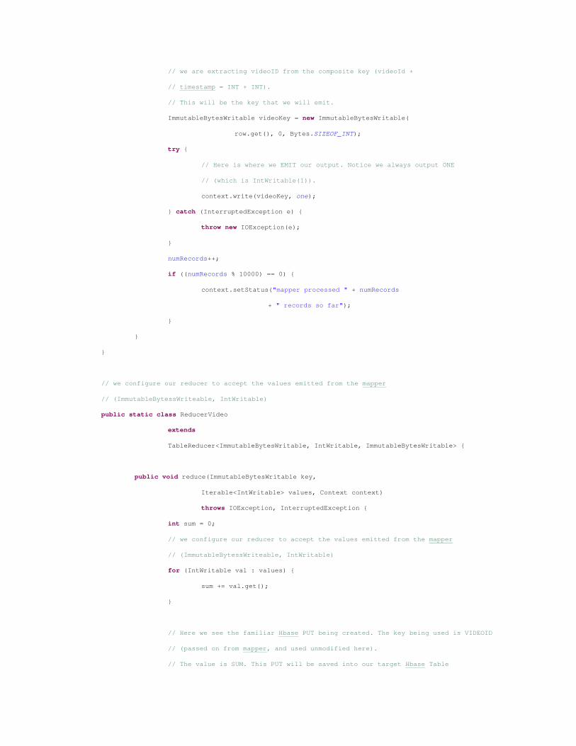
// we are extracting videoID from the composite key (videoId +
// timestamp = INT + INT).
// This will be the key that we will emit.
ImmutableBytesWritable videoKey = new ImmutableBytesWritable(
row.get(), 0, Bytes.SIZEOF_INT);
try {
// Here is where we EMIT our output. Notice we always output ONE
// (which is IntWritable(1)).
context.write(videoKey, one);
} catch (InterruptedException e) {
throw new IOException(e);
}
numRecords++;
if ((numRecords % 10000) == 0) {
context.setStatus("mapper processed " + numRecords
+ " records so far");
}
}
}
// we configure our reducer to accept the values emitted from the mapper
// (ImmutableBytessWriteable, IntWritable)
public static class ReducerVideo
extends
TableReducer<ImmutableBytesWritable, IntWritable, ImmutableBytesWritable> {
public void reduce(ImmutableBytesWritable key,
Iterable<IntWritable> values, Context context)
throws IOException, InterruptedException {
int sum = 0;
// we configure our reducer to accept the values emitted from the mapper
// (ImmutableBytessWriteable, IntWritable)
for (IntWritable val : values) {
sum += val.get();
}
// Here we see the familiar Hbase PUT being created. The key being used is VIDEOID
// (passed on from mapper, and used unmodified here).
// The value is SUM. This PUT will be saved into our target Hbase Table
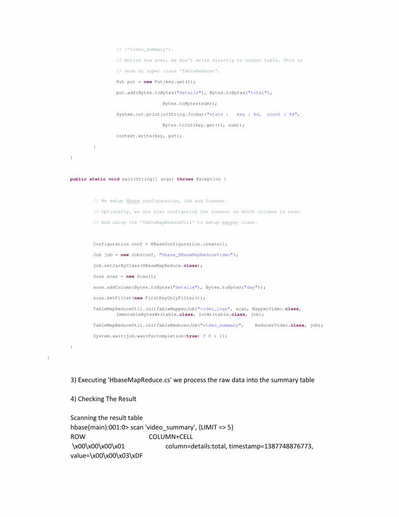
// ('video_summary').
// Notice how ever, we don't write directly to output table. This is
// done by super class 'TableReducer'.
Put put = new Put(key.get());
put.add(Bytes.toBytes("details"), Bytes.toBytes("total"),
Bytes.toBytes(sum));
System.out.println(String.format("stats : key : %d, count : %d",
Bytes.toInt(key.get()), sum));
context.write(key, put);
}
}
public static void main(String[] args) throws Exception {
// We setup Hbase configuration, Job and Scanner.
// Optionally, we are also configuring the scanner on which columns to read.
// And using the 'TableMapReduceUtil' to setup mapper class.
Configuration conf = HBaseConfiguration.create();
Job job = new Job(conf, "Hbase_HBaseMapReduceVideo");
job.setJarByClass(HBaseMapReduce.class);
Scan scan = new Scan();
scan.addColumn(Bytes.toBytes("details"), Bytes.toBytes("day"));
scan.setFilter(new FirstKeyOnlyFilter());
TableMapReduceUtil.initTableMapperJob("video_logs", scan, MapperVideo.class,
ImmutableBytesWritable.class, IntWritable.class, job);
TableMapReduceUtil.initTableReducerJob("video_summary", ReducerVideo.class, job);
System.exit(job.waitForCompletion(true) ? 0 : 1);
}
}
3) Executing 'HbaseMapReduce.cs' we process the raw data into the summary table
4) Checking The Result
Scanning the result table
hbase(main):001:0> scan 'video_summary', {LIMIT => 5}
ROW COLUMN+CELL
\x00\x00\x00\x01 column=details:total, timestamp=1387748876773,
value=\x00\x00\x03\xDF
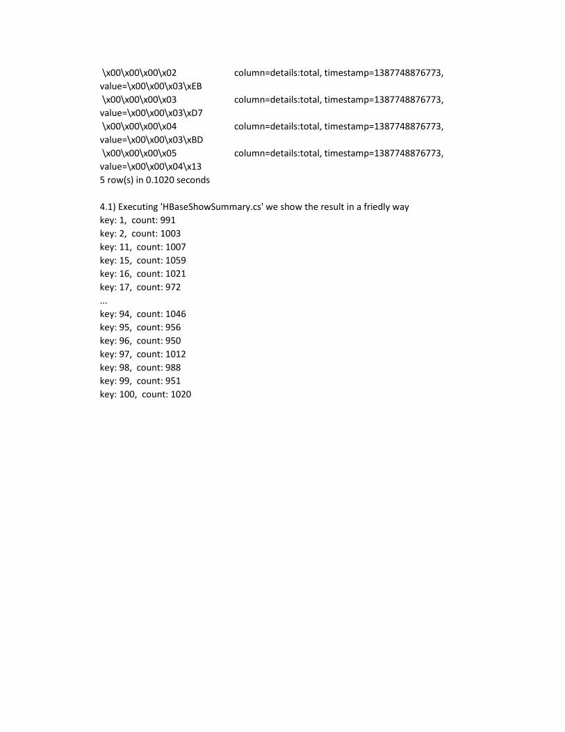
\x00\x00\x00\x02 column=details:total, timestamp=1387748876773,
value=\x00\x00\x03\xEB
\x00\x00\x00\x03 column=details:total, timestamp=1387748876773,
value=\x00\x00\x03\xD7
\x00\x00\x00\x04 column=details:total, timestamp=1387748876773,
value=\x00\x00\x03\xBD
\x00\x00\x00\x05 column=details:total, timestamp=1387748876773,
value=\x00\x00\x04\x13
5 row(s) in 0.1020 seconds
4.1) Executing 'HBaseShowSummary.cs' we show the result in a friedly way
key: 1, count: 991
key: 2, count: 1003
key: 11, count: 1007
key: 15, count: 1059
key: 16, count: 1021
key: 17, count: 972
...
key: 94, count: 1046
key: 95, count: 956
key: 96, count: 950
key: 97, count: 1012
key: 98, count: 988
key: 99, count: 951
key: 100, count: 1020
7777 MMMMARKARKARKARKET ET ET ET AAAADAPTATIONDAPTATIONDAPTATIONDAPTATION
Compared to the other NoSql players in the market, HBase is considered one of the most used and
deployed data bases in the BigData arena given the fact that it is utilizing Hadoop which in turn already
established its market position as a BigData platform. Currently there are many well-known customers
with a significant HBase cluster installed such as Adobe, Careers.rs, meetup, Twitter, VideoSurf , Yahoo
and WorldLingo.
Moreover, In November 2010, Facebook launched its first production usage of the HBase NoSQL-style
database to power its messages storage. Since then, it was scaled up and spread out inside Facebook.
This specific adaptation is considered to be a huge prove of HBase capabilities, not only because
Facebook requires manipulation of massive social data, but also because Facebook is the one who
started project “Casendra” which is considered one of the major alternatives\competitors of HBase.
8888 CCCCOMPLEMENTING THE STAOMPLEMENTING THE STAOMPLEMENTING THE STAOMPLEMENTING THE STACKCKCKCK
It’s worth mentioning that the open-source community, especially Apache, is contributing to the NoSQL
movement non stopping. Currently there are several projects running to improve or add new
capabilities to the existing platforms like Hadoop (one can consider that HBase itself is one these
projects complementing Hadoop with random data access).
The flowing list will briefly introduce other projects in the Hadoop ecosystem and highlights new
investigation topics for next academic projects
- Drill: Introducing real-time real-time querying of nested data and to scale to clusters of 10,000
nodes or more, modeled after Google Dremel.
- Flume: Considered the ETL tool for Hadoop, It’s a tool for harvesting, aggregating and moving
large amounts of log data in and out of Hadoop. Flume "channels" data between "sources" and
"sinks" and its data harvesting can either be scheduled or event-driven. Possible sources for
Flume include Avro, files, and system logs, and possible sinks include HDFS and HBase.
- Hive: Hive provides a warehouse structure and SQL-like access for data in HDFS and other
Hadoop input sources (e.g. Amazon S3). Hive's query language, HiveQL, compiles to MapReduce.
It also allows user-defined functions (UDFs). Hive is widely used, and has itself become a "sub-
platform" in the Hadoop ecosystem.
- Pig: Is a framework consisting of a high-level scripting language (Pig Latin) and a run-time
environment that allows users to execute MapReduce on a Hadoop cluster. Like HiveQL in Hive,
Pig Latin is a higher-level language that compiles to MapReduce.
- Mahout: Mahout is a scalable machine-learning and data mining library. Algorithms in the
Mahout library belong to the subset that can be executed in a distributed fashion, and have
been written to be executable in MapReduce.
9999 SSSSUMMARYUMMARYUMMARYUMMARY
In this report we investigated one of the major movements in the IT industry nowadays which is
“NoSQL” that is usually coupled with the buzz word “BigData”. We have seen the history and evolution
of DBMSs and data storage needs from RDBMS to the current days of massive data sets that requires
new techniques in data storage and manipulation.
We discussed the common characteristics- such as Non-relational, schema-less, cluster friendly - that
can be found in the NoSQL databases in general that mainly decide our choice between using a
relational versus a NoSQL database. And then we went through the different families of NoSQL that
defines the data storage methodology of each of them (key-value, document, graph, column and wide-
column families)
After the NoSQL Introduction, we analyzed the Hadoop platform, consisting mainly of a distributed file
system (HDFS) coupled with a distributed programming framework, MapReduce, to process such data
hosted on the HDFS in an efficient manner.
We then started focusing on one database management system, HBase, which is a wide-column NoSQL
database based on the Hadoop platform, mainly providing it with random read\write access and
database management features addressing scalability issues. We also discussed some of the internals of
HBase in terms of logical and physical data architecture, how it is addressing scalability by table
sharding, available operations using HBase Shell and Java API, ACID semantics and how to run
MapReduce programs on it.
Finally, we ended the report by talking about the wide and fast adoption of HBase in major organizations
that are well known of handling massive amounts of data, proving that there is actually a big market for
NoSQL databases in general and HBase in particular. And finally we listed some other interesting
projects in the Hadoop ecosystem that can enrich the Hadoop\HBase stack and can also be hot-topics
for further investigations (or may be contribution) in the Hadoop domain.
Based on this technology investigation, we can confidently conclude that NoSQL databases are not
applicable for every use-case and it’s definitely not a replacement for Relational DBMSs but rather a new
branch of database technologies that address specific requirements (mainly handling extremely larger
and\or semi-structured datasets) at the cost of compromising other features that were taken for
granted in the relational world. Nevertheless, inside the NoSQL domain, Hadoop and HBase are clearly
market leaders with a lot of potential in the BigData world that should be top listed for consideration
once an organization realizes its need for a wide-column NoSql database, And even though the
MapReduce programing framework may seems harder to learn and adapt, there is a rich portfolio of
open source projects that complements Hadoop & HBase with SQL like query language - like Hive & Pig-
that are already widely adapted and supported in the HBase market.
10101010 RRRREFERENCESEFERENCESEFERENCESEFERENCES
1. http://hbase.apache.org/acid-semantics.html
2. http://www.zdnet.com/rdbms-vs-nosql-how-do-you-pick-7000020803/
3. NoSQL by Greg Burd
4. http://www.aerospike.com/what-is-a-nosql-key-value-store/
5. Relational Databases, Object Databases, Key-Value Stores,
Document Stores, and Extensible Record Stores: A Comparison
Rick Cattell December 2010
6. http://www.tomsitpro.com/articles/rdbms-sql-cassandra-dba-developer,2-547-2.html
7. Google Paper: MapReduce: Simplified Data Processing on Large Clusters, Dean and
Chemawat
8. Hbase logical table: Intro to Hbase slides
9. http://en.wikipedia.org/wiki/Column-oriented_DBMS
10. http://hbase.apache.org/acid-semantics.html
11. http://wiki.apache.org/hadoop/Hbase/PoweredBy
12. http://ebookbrowsee.net/mapred-tutorial-pdf-d422671722
13. https://hadoop.apache.org/docs/r1.2.1/mapred_tutorial.html
14. http://hadoop.apache.org/docs/r0.19.0/mapred_tutorial.pdf
15. http://dbmsmusings.blogspot.be/2010/03/distinguishing-two-major-types-of_29.html
16. http://www.revelytix.com/?q=content/hadoop-ecosystem
17. Introduction to NoSQL by Martin Fowler (Youtube)
18. Intro to HBase, Alex Baranau, Sematext Internation 2012