Exploring Full-Duplex Gains in Multi-Cell Wireless Networks:A Spatial Stochastic Framework

Shu Wang, Vignesh Venkateswaran and Xinyu ZhangUniversity of Wisconsin-Madison

Email: swang367,vvenkateswar@wisc.edu xyzhang@ece.wisc.edu

Abstract—Full-duplex radio technology is becoming mature andholds potential to boost the spectrum efficiency of a point-to-point wireless link. However, a fundamental understanding isstill lacking, with respect to its advantage over half-duplex inmulti-cell wireless networks with contending links. In this paper,we establish a spatial stochastic framework to analyze the meannetwork throughput gain from full-duplex, and pinpoint the keyfactors that determine the gain. Our framework extends classicalstochastic geometry analysis with a new tool-set, which allows us tomodel a trade-off between the benefit from concurrent full-duplextransmissions and the loss of spatial reuse, particularly for CSMA-based transmitters with random backoff. The analysis derivesclosed-form expressions for the full-duplex gain as a function oflink distance, interference range, network density, and carriersensing schemes. It can be easily applied to guide the deploymentchoices during the early stage of network planning.

I. INTRODUCTION

Recent advances in radio hardware and signal processing arepushing full-duplex wireless communications close to commer-cialization [1]. However, existing work mostly focused on full-duplex PHY-layer implementation [2], [3] or MAC protocols[4], [5] that extend 802.11 CSMA/CA. Unlike half-duplexwireless networks whose asymptotics have been investigatedextensively [6], the fundamental network-capacity implicationsof full-duplex remain largely underexplored.

In distributed wireless networks, contending nodes’ trans-missions need to be separated in time, frequency, and/or spaceto avoid excessive interference. Whereas full-duplex allows apair of nodes to co-locate their transmissions in the same timeslot and frequency band, their spatial interference footprint isheavier than a half-duplex pair. An accurate characterizationof this trade-off can lead to a fundamental understanding ofthe full-duplex network capacity and the achievable gain, thusguiding the practical protocol design and network deployment.

The objective of this work is to provide an analytical frame-work allowing one to access the key properties of full-duplexwireless networks running carrier-sensing based random accessprotocols. The insights we seek to obtain include, e.g., whatis the network throughput (gain) when using full-duplex radioscompared with half-duplex ones? What are the key factors thatdetermine the gain and how to engineer such design knobsto maximize full-duplex’s potential? With this framework, wealso seek to derive general guidelines for deploying full-duplexmulti-cell wireless LANs, e.g., for an anticipated AP density,which type of radio is more cost-effective?

For such an analytical model, the main challenge lies in aneed to take into account interference, random contention, andthe resulting spatial reuse among contending links. Such fac-tors, of course, are topology dependent. One cannot traverse theenormous number of possible configurations, but must instead

consider a statistical spatial model for the node locations, andextracts insights from there.

Following this principle, we assume certain statistical dis-tribution of AP/client locations, and derive spatial averages ofcritical network quantities, e.g., interference and spatial densityof successful transmitters. Such a spatial averaging technique,widely referred to as stochastic geometry [7], has been used in avariety of wireless network examples, like ad-hoc networks, inorder to perform average-case analysis of network throughput,by modeling the interference experienced by nodes under arandom access MAC protocol.

It is, however, non-trivial to apply the classical stochasticgeometry model to full-duplex networks, because of two newbarriers. First, existing stochastic geometry analysis [8], [9]uses a hard-core point process (HCPP) to model the distributionof winning transmitters. The contention region of a point inHCPP is defined by a unit disc containing no other points. Withfull-duplex, the spatial footprint of two neighboring transmit-ters can become correlated, which can no longer be handledby conventional stochastic geometry models. Second, existingmodels only focus on winning transmitters after CSMA/CAcontention, but ignore the receiver which itself has an exclusiveregion and is vulnerable to artifacts of carrier sensing such ashidden terminals. Such artifacts are critical to spatial reuse andto the real gain from full-duplex.

In light of the above challenges, we propose a new stochasticframework that can analyze the average spatial footprint of atypical full-duplex pair, as well as the spatial distribution of full-duplex pairs that win contention. Our approach leads to closed-form expressions for the average throughput of full-duplexnetworks with Poisson-bipolar distributed links. It also enablesclosed-form analysis of half-duplex throughput under carriersensing artifacts, e.g., hidden/exposed terminals. Consequently,we can derive the full-duplex throughput gain under a varietyof topological parameters and protocol imperfectness.

We find that the most critical factor that determines full-duplex gain is the mean link distance d relative to the carriersensing range. A smaller d amplifies full-duplex gain since,intuitively, it reduces the interference footprint of a full-duplexlink. For a fixed d, full-duplex gain tends to be larger in avery sparse deployment of APs, yet the gain saturates quicklyas density increases. More interestingly, we found a majorcontributing factor to full-duplex gain lies in full-duplex nodes’capability to implicitly remove hidden/exposed terminals. Thus,the full-duplex gain tends to be amplified under imperfect car-rier sensing. In addition, we show that our analytical frameworkcan be applied to guide the choice between full-duplex or half-duplex technologies during deployment stage, given various

2

(a) (b)

Primary transmitter

Secondary transmitter Transmitter Primary

receiverSecondary

receiver

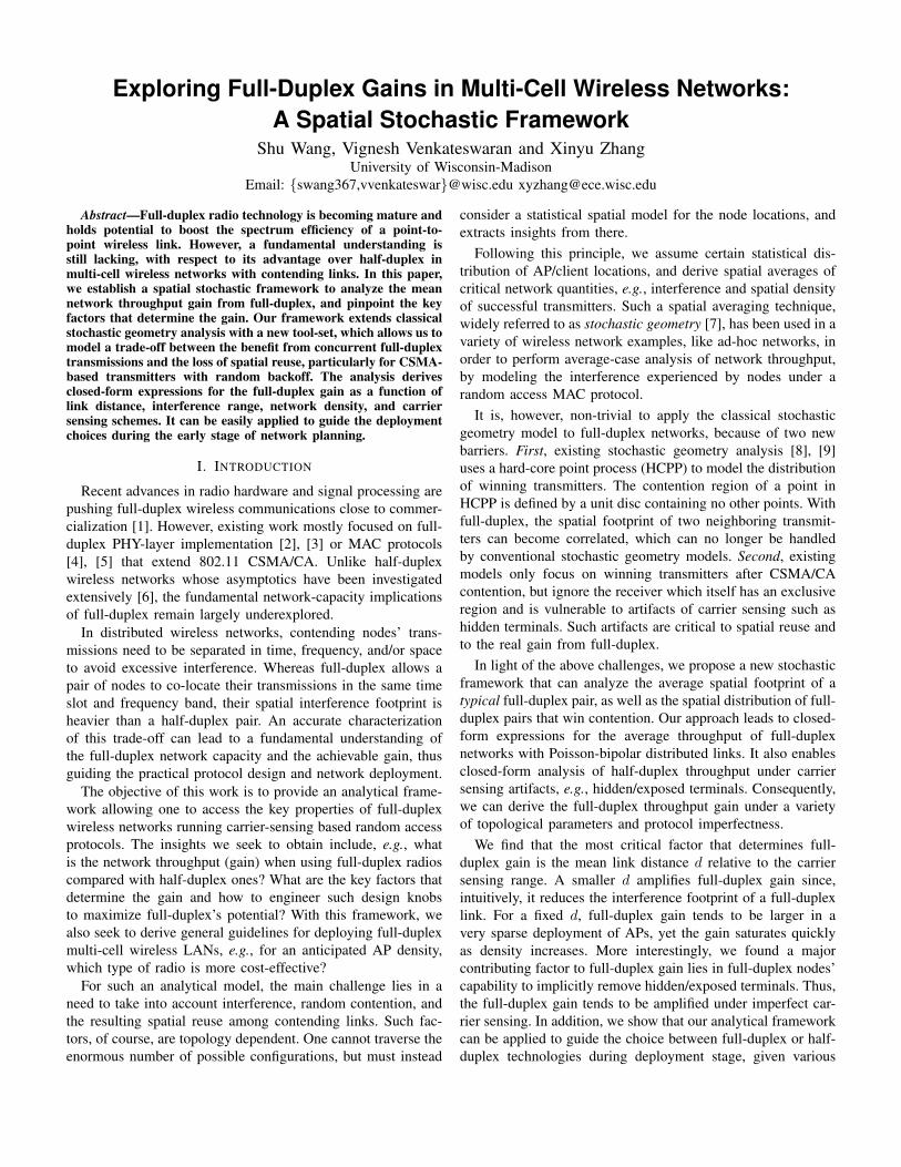
Fig. 1. Full-duplex transmission modes in a wireless LAN: (a) bidirectionaltransmission and (b) cut-through transmission.

objectives and constraints, e.g., client/AP density and cost ofhalf- and full-duplex radio.

The rest of this paper is structured as follows. We first presenta background on stochastic geometry and our network modelsin Sec. II. Then we analyze the full-duplex gain under two setsof interference models, in Sec. III and IV. In Sec. V, we applyour models to full-duplex network planning. Sec. VI discussesrelated work and finally, Sec. VII concludes the paper.

II. BACKGROUND AND OVERVIEW OF NETWORK MODELS

In this section, we present the essential models and assump-tions underlying our analytical framework.

A. A Primer on Stochastic Geometry and Its Limitations

Stochastic geometry provides average-case analysis of net-work throughput, wherein the averages are made over a largenumber of nodes randomly located in the spatial domain.Recent stochastic geometry models of 802.11 CSMA networkscommonly apply a two-step approach [8]. First, nodes areassumed to be deployed following a Poisson Point Process(PPP). Then, the distribution of simultaneously active trans-mitters after CSMA contention is approximated by a Maternhard core point process (HCPP). Simply put, the HCPP thinsthe parent PPP and models the winning nodes after randombackoff. Second, the interference experienced by a typicalwinning node is approximated by the interference resultingfrom a PPP which has the same intensity as the HCPP. Suchapproximation has been shown to be fairly accurate, mainlybecause the exact locations of the active transmitters matter lessthan the number of other active transmitters (interferers) andtheir relative distances. Given the approximated HCPP, networkperformance metrics such as transmission success probability(under interference) and throughput can be easily derived.

When applied to modeling the full-duplex gain, existingstochastic geometry models fall short of accuracy from threeaspects. (i) They mainly focus on potential transmitters througha homogeneous point process model. The spatial reuse be-tween transmitters and receivers cannot be modeled but isthe most critical factor that determines the full-duplex gain[10]. (ii) They assume a unit disk exclusive region aroundeach transmitter, and omit the carrier sensing artifacts, suchas exposed and hidden terminals, which again account forthe discrepancies in theoretical and practical limit of bothhalf-duplex and full-duplex networks. (iii) They commonlyapproximate the received signal-to-interference-plus-noise ratio(SINR) using the SINR at the transmitter side, yet whether atransmission succeeds depends SINR at the receiver side (orboth sides for full-duplex).

We remedy the above limitations by marrying stochasticgeometry with the two interference models proposed in Gupta

(a)

θ θ

(b) (c)

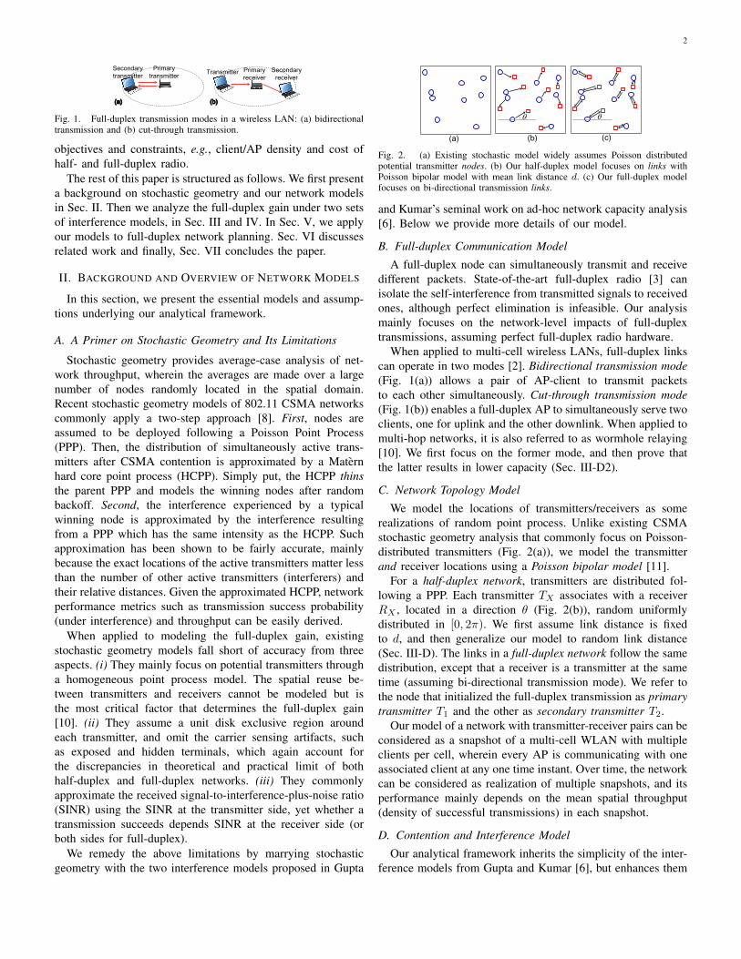
Fig. 2. (a) Existing stochastic model widely assumes Poisson distributedpotential transmitter nodes. (b) Our half-duplex model focuses on links withPoisson bipolar model with mean link distance d. (c) Our full-duplex modelfocuses on bi-directional transmission links.

and Kumar’s seminal work on ad-hoc network capacity analysis[6]. Below we provide more details of our model.

B. Full-duplex Communication Model

A full-duplex node can simultaneously transmit and receivedifferent packets. State-of-the-art full-duplex radio [3] canisolate the self-interference from transmitted signals to receivedones, although perfect elimination is infeasible. Our analysismainly focuses on the network-level impacts of full-duplextransmissions, assuming perfect full-duplex radio hardware.

When applied to multi-cell wireless LANs, full-duplex linkscan operate in two modes [2]. Bidirectional transmission mode(Fig. 1(a)) allows a pair of AP-client to transmit packetsto each other simultaneously. Cut-through transmission mode(Fig. 1(b)) enables a full-duplex AP to simultaneously serve twoclients, one for uplink and the other downlink. When applied tomulti-hop networks, it is also referred to as wormhole relaying[10]. We first focus on the former mode, and then prove thatthe latter results in lower capacity (Sec. III-D2).

C. Network Topology Model

We model the locations of transmitters/receivers as somerealizations of random point process. Unlike existing CSMAstochastic geometry analysis that commonly focus on Poisson-distributed transmitters (Fig. 2(a)), we model the transmitterand receiver locations using a Poisson bipolar model [11].

For a half-duplex network, transmitters are distributed fol-lowing a PPP. Each transmitter TX associates with a receiverRX , located in a direction θ (Fig. 2(b)), random uniformlydistributed in [0, 2π). We first assume link distance is fixedto d, and then generalize our model to random link distance(Sec. III-D). The links in a full-duplex network follow the samedistribution, except that a receiver is a transmitter at the sametime (assuming bi-directional transmission mode). We refer tothe node that initialized the full-duplex transmission as primarytransmitter T1 and the other as secondary transmitter T2.

Our model of a network with transmitter-receiver pairs can beconsidered as a snapshot of a multi-cell WLAN with multipleclients per cell, wherein every AP is communicating with oneassociated client at any one time instant. Over time, the networkcan be considered as realization of multiple snapshots, and itsperformance mainly depends on the mean spatial throughput(density of successful transmissions) in each snapshot.

D. Contention and Interference Model

Our analytical framework inherits the simplicity of the inter-ference models from Gupta and Kumar [6], but enhances them

3

(a)

(d)

Reusable by other RX

Reusable by other TX

Unreusable by other T1/T2 (no hidden or exposed terminals )

(b)

Reusable by other RX

Unreusable by other TX(Exposed terminal problem may exist)

Hidden terminals may

exist

(c)

Reusable by other RX

Unreusable by other TX(Exposed terminal problem may exist)

Hidden terminals may

still exist

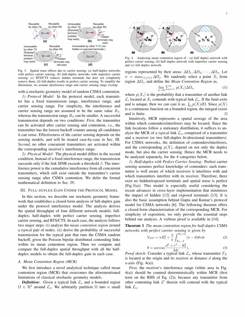
Fig. 3. Spatial reuse effects due to carrier sensing: (a) half-duplex networkswith perfect carrier sensing; (b) half-duplex networks with imperfect carriersensing; (c) RTS/CTS reduces hidden terminals but does not completelyremove them; (d) full-duplex results in perfect carrier sensing. To simplify theillustration, we assume interference range and carrier sensing range overlap.

with a stochastic geometry model of random CSMA contention.1) Protocol Model: In the protocol model, each transmit-

ter has a fixed transmission range, interference range, andcarrier sensing range. For simplicity, the interference andcarrier sensing range are assumed to be the same value RI ,whereas the transmission range RS can be smaller. A successfultransmission depends on two conditions: First, the transmittercan be activated after carrier sensing and contention, i.e., thetransmitter has the lowest backoff counter among all candidatesit can sense. Effectiveness of the carrier sensing depends on thesensing models, and will be treated case-by-case in Sec. III.Second, no other concurrent transmitters are activated withinthe corresponding receiver’s interference range.

2) Physical Model: The physical model differs in the secondcondition. Instead of a fixed interference range, the transmissionsucceeds only if the link SINR exceeds a threshold β. The inter-ference power is the cumulative interference from all concurrenttransmitters, which still exist outside the transmitter’s carriersensing range after CSMA contention. We defer the formalmathematical definition to Sec. IV.

III. FULL-DUPLEX GAIN UNDER THE PROTOCOL MODEL

In this section, we describe our stochastic geometry frame-work that establishes a closed-form analysis of full-duplex gainunder the protocol interference model. The analysis derivesthe spatial throughput of four different network models: full-duplex; half-duplex with perfect carrier sensing, imperfectcarrier sensing, and RTS/CTS. In each case, the analysis followstwo major steps: (i) analyze the mean contention region arounda typical pair of nodes. (ii) derive the probability of successfultransmission for the typical pair that runs the CSMA randombackoff, given the Poisson bipolar distributed contending linkswithin its mean contention region. Then we compute andcompare the full-duplex spatial throughput with all the half-duplex models to obtain the full-duplex gain in each case.

A. Mean Contention Region (MCR)

We first introduce a novel analytical technique called meancontention region (MCR) that overcomes the aforementionedlimitations of classical stochastic geometry models.

Definition: Given a typical link Lo and a bounded regionΩ ∈ R2 around Lo. We arbitrarily partition Ω into n small

Rxd

Tx’

Rx’

d

Tx Tx Rxd

T2

d

T1

θ

d

θ

Tx’

Rx’

(a) (b) (c)

Fig. 4. Analyzing mean contention region of : (a) half duplex network withperfect carrier sensing, (b) half duplex network with imperfect carrier sensingand (c) full duplex network.

regions represented by their areas: ∆Ω1,∆Ω2, · · · ,∆Ωn. Letσ = max1≤j≤n ∆Ωj . We randomly select a point Xi fromregion ∆Ωi, and define the Mean Contention Region as,

limσ→0

∑ni=1 p(Xi)∆Ωi, (1)

where p(Xi) is the probability that a transmitter of another linkLi located at Xi contends with typical link Lo. If the limit exitsand is unique, then we can cast it as:

∫Ωp(X)dΩ. Since p(X)

is a continuous function on a bounded region, the integral existsand is finite. ut

Intuitively, MCR represents a spatial average of the areawithin which contenders/interferers may be located. Since thelink locations follow a stationary distribution, it suffices to an-alyze the MCR of a typical link Lo, comprised of a transmitterand a receiver (or two full-duplex bi-directional transmitters).For CSMA networks, the definition of contenders/interferers,and the corresponding p(X), depend on not only the duplexmode, but also the carrier sensing. Hence the MCR needs tobe analyzed separately, for the 4 categories below.

1) Half-duplex with Perfect Carrier Sensing: Perfect carriersensing assumes perfect knowledge of contenders: each trans-mitter is well aware of which receivers it interferes with andwhich transmitters interfere with its receiver. Therefore, thereexist no hidden/exposed terminals and spatial reuse is perfect(Fig.3(a)). This model is especially useful considering therecent advances in cross-layer implementation that minimizesthe impact of hidden [12] and exposed terminals [13]. It isalso the basic assumption behind Gupta and Kumar’s protocolmodel for CSMA networks [6]. The following theorem offersa closed-form characterization of the corresponding MCR. Forsimplicity of exposition, we only provide the essential stepsbehind our analysis. A verbose proof is available in [14].

Theorem 1 The mean contention region for half-duplex CSMAnetworks with perfect carrier sensing is given by

VHP = πR2I +

2

π

∫ RI+d

RI−d(π − θ)θrdr (2)

θ = arccos(d2 + r2 −R2

I

2dr). (3)

Proof sketch: Consider a typical link Lo whose transmitter TXis located at the origin and its receiver at distance d along thex-axis (Fig. 4(a)).

First, the receiver’s interference range (white area in Fig.4(a)) should be counted deterministically within MCR (firstterm on the RHS of Eq. (2)), because any transmitter fromother contenting link L′ therein will contend with the typicallink Lo.

4

Second, consider a contending link L′ whose transmitter TX′is within the shaded area in Fig. 4(a). If its receiver RX′ islocated within the interference range of TX (red solid arc), thenRX′ will be interfered. Otherwise (green dashed arc), it needsnot contend with the typical link and can transmit concurrentlyunder perfect carrier sensing. Under Poisson bipolar model,the orientation of a receiver w.r.t. its transmitter is uniformlydistributed in [0, 2π). Thus, we can obtain the probability ofRX′ located in TX ’s interference range by calculating theratio of θ to 2π. Since this probability p(X) depends onthe transmitter’s location, we can integrate the probabilitythroughout the shaded area to obtain the spatial average (secondterm on the RHS of Eq. (2)).

For any other transmitter outside the above two regions, itsreceiver RX′ can never fall within TX ’s interference range, andthus it should not be counted into the MCR. ut

2) Half-duplex with Imperfect Carrier Sensing: In the basic802.11 protocol (Fig. 3(b)), a node defers its transmissionwhenever it senses a busy channel. This mechanism reducesthe risk of collision but often leads to the exposed terminalproblem, i.e., some nodes may not interfere a receiver, butare unnecessarily suppressed by the corresponding transmitter.In addition, it suffers from the hidden terminal problem, i.e.,other nodes outside the ongoing transmitter’s carrier sensingrange but inside the ongoing receiver’s interference range canstill cause collisions. We refer to this category of protocol asimperfect carrier sensing, and analyze the MCR as follows.Theorem 2 Under imperfect carrier sensing, the mean con-tention region for CSMA networks is given by

VHI = Vu +2

π

∫ RI+d

RI

(π − θ)θrdr (4)

Vu = 2πR2I − 2R2

I arccos(d

2RI) + d

√R2I −

d2

4(5)

θ = arccos(d2 + r2 −R2

I

2dr

)(6)

Proof sketch: The transmitter TX suppresses all other trans-mitters within its interference range which, together with thereceiver’s interference range, become a deterministic contentionregion (the Vu term above, corresponding to the white region inFig. 4(b)). Spatial average of contention region for the shadedarea can be derived in a similar way to Theorem 1. ut

3) Half-duplex with RTS/CTS Signaling: An enhanced ver-sion of 802.11 uses RTS/CTS to alleviate hidden terminals(Fig. 3(c)). Yet it still bears the exposed terminal problem.Moreover, there may still be hidden terminals outside the CTStransmission range but within the receiver’s interference range.Denote the transmission range as RS , then we can derive theMCR under RTS/CTS signaling as follows.Theorem 3 The mean contention region for half duplex net-work using RTS/CTS is given by

VHRC =

V1 + V2 + V3 + 2(V4 − V5) d > RI −RSVHI d ≤ RI −RS

(7)

V1 = 2πR2I − 2R2

I arccos(d

2RI) + d

√R2I −

d2

4(8)

V2 =2

π

∫ RI+d

RI

(π − γ1 − θ2)θ1rdr (9)

V3 =2

π

∫ RS+d

RI

(π − γ2 − θ3)θ4rdr (10)

V4 =1

2π

∫ d

0

∫ π−θ6+γ1

θ5−γ2

(ϕ1 + ϕ2 + ϕ3)rdrdθ (11)

V5 =1

2π

∫ RI

RS

∫ π−γ2−θ3

π−θ1(ϕ4 + ϕ5 + θ4)rdrdθ (12)

The γ1, γ2, θ1 to θ5 and ϕ1 to ϕ5 are intermediate parameters.Detailed expressions are put in [14] for simplicity of exposition.

The proof follows similar steps as the full-duplex case below,and is thus omitted to avoid redundancy.

4) Full-duplex: For full-duplex links, we assume a carriersensing model similar to the FuMAC in [15]. A bi-directionalfull-duplex transmission can start only if both the primary andsecondary transmitter sense an idle channel. Such synchronousfull-duplex scheme has proven to have superior performancethan one that mixes half-duplex with full-duplex transmissions[15]. In addition, (i) it eliminates hidden terminals becauseevery receiver is a transmitter at the same time that uses itstransmission as a busy-tone to protect itself from interferers. (ii)exposed terminals no longer exists, because no transmitter cancoexist with other transmitter (and simultaneously a receiver)within the carrier sensing range anyway (Fig. 3(d)).

In other words, full-duplex carrier sensing implicitly removesthe hidden/exposed terminals. Our later analysis will show thatthis is where the main benefit of full-duplex comes from. Underthis protocol, the MCR can be characterized as follows.Theorem 4 The mean contention region for a typical full-duplex link is given by

VF = V1 + 2V2 + 2V3 (13)

V1 = 2πR2I − 2R2

I arccos(d

2RI) + d

√R2I −

d2

4(14)

V2 =2

π

∫ RI+d

RI

(π − θ2 − θ3)θ1rdr (15)

V3 =

∫ d

0

∫ 3π − 2θ4 − θ5

22θ4 + θ5 − π

2

(ϕ1 + ϕ2 + ϕ3

2π)rdrdθ (16)

where θ1 to θ5, ϕ1 to ϕ3, and δ1 to δ2 are intermediateparameters whose detailed expressions are available in [14].Proof sketch: We consider three regions shown as differentpatterns in Fig. 4(c). The white region is a deterministiccontention region, whereas other two contribute to the MCRprobabilistically, and can be analyzed using a similar procedureas in Theorem 1. The detailed proof is put in [14]. ut

B. Spatial Density of Successful Transmissions

We now derive the mean transmission density, i.e., averagenumber of successful transmissions per unit area, after thetypical pair of nodes contend with peers in the MCR. TheCSMA contention (Sec. II) can be modeled as a Matern Type IIprocess [16] that thins the original PPP distributed contenderswithin the MCR. Given a stationary independently marked PPPof intensity µ, the Palm retaining probability that a point x

5

0

0.5

1

1.5

2

2.5

3

0 20 40 60 80 100

λ HP

(m-2

)

d (m)

x 10-5

n=1

n=10

TheoreticalSimulation

0

0.5

1

1.5

2

2.5

3

0 20 40 60 80 100

λ F(m

-2)

d (m)

x 10-5

n=1

n=10

TheoreticalSimulation

(a) (b)

(c) (d)

0

0.5

1

1.5

2

2.5

3

0 20 40 60 80 100

λ HI(m

-2)

d (m)

x 10-5

n=1

n=10

TheoreticalSimulation

0

0.5

1

1.5

2

2.5

3

0 20 40 60 80

λ HR

C(m

-2)

d (m)

x 10-5

n=1

n=10

TheoreticalSimulation

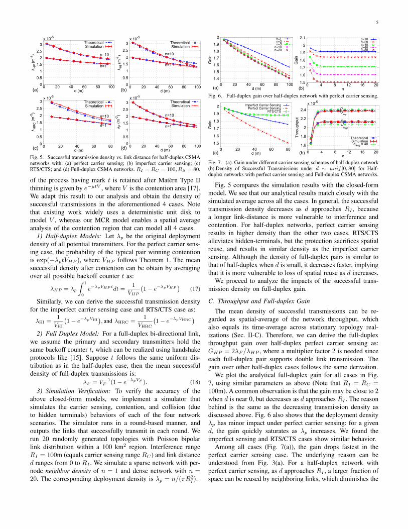
Fig. 5. Successful transmission density vs. link distance for half-duplex CSMAnetworks with: (a) perfect carrier sensing; (b) imperfect carrier sensing; (c)RTS/CTS; and (d) Full-duplex CSMA networks. RI = RC = 100, RS = 80.

of the process having mark t is retained after Matern Type IIthinning is given by e−µtV , where V is the contention area [17].We adapt this result to our analysis and obtain the density ofsuccessful transmissions in the aforementioned 4 cases. Notethat existing work widely uses a deterministic unit disk tomodel V , whereas our MCR model enables a spatial averageanalysis of the contention region that can model all 4 cases.

1) Half-duplex Models: Let λp be the original deploymentdensity of all potential transmitters. For the perfect carrier sens-ing case, the probability of the typical pair winning contentionis exp(−λptVHP ), where VHP follows Theorem 1. The meansuccessful density after contention can be obtain by averagingover all possible backoff counter t as:

λHP = λp

∫ 1

0

e−λpVHP tdt =1

VHP

(1− e−λpVHP

)(17)

Similarly, we can derive the successful transmission densityfor the imperfect carrier sensing case and RTS/CTS case as:

λHI =1

VHI

(1− e−λpVHI

), and λHRC =

1

VHRC

(1− e−λpVHRC

)2) Full Duplex Model: For a full-duplex bi-directional link,

we assume the primary and secondary transmitters hold thesame backoff counter t, which can be realized using handshakeprotocols like [15]. Suppose t follows the same uniform dis-tribution as in the half-duplex case, then the mean successfuldensity of full-duplex transmissions is:

λF = V −1F (1− e−λpVF ). (18)

3) Simulation Verification: To verify the accuracy of theabove closed-form models, we implement a simulator thatsimulates the carrier sensing, contention, and collision (dueto hidden terminals) behaviors of each of the four networkscenarios. The simulator runs in a round-based manner, andoutputs the links that successfully transmit in each round. Werun 20 randomly generated topologies with Poisson bipolarlink distribution within a 100 km2 region. Interference rangeRI = 100m (equals carrier sensing range RC) and link distanced ranges from 0 to RI . We simulate a sparse network with per-node neighbor density of n = 1 and dense network with n =20. The corresponding deployment density is λp = n/(πR2

I).

1.4

1.5

1.6

1.7

1.8

1.9

2

0 20 40 60 80 100

Gai

n

d (m)

n=1n=2n=3

n=10n=20

1.5

1.6

1.7

1.8

1.9

2

2.1

0 4 8 12 16 20

Gai

n

n

d=10d=20d=40d=60d=80

(a) (b)

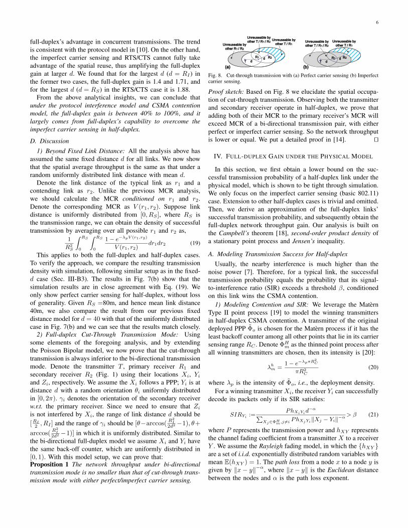
Fig. 6. Full-duplex gain over half-duplex network with perfect carrier sensing.

1.6

1.8

2

2.2

2.4

0 4 8 12 16 20

Throu

ghpu

t

n

x 10-5

λF

λHP

TheoreticalSimulationdavg = 401.5

1.6

1.7

1.8

1.9

2

0 20 40 60 80

Gain

d (m)

Imperfect Carrier SensingPerfect Carrier Sensing

RTS/CTS

(a) (b)

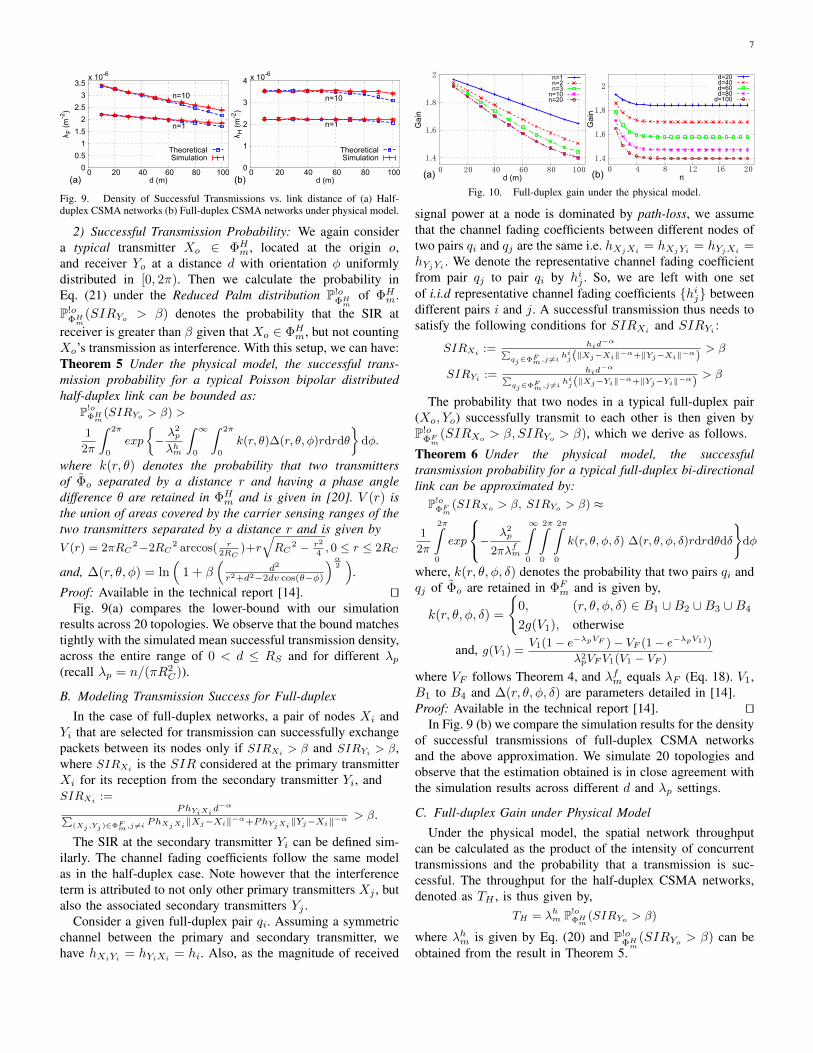
Fig. 7. (a). Gain under different carrier sensing schemes of half duplex network(b).Density of Successful Transmissions under d ∼ unif [0, 80] for Half-duplex networks with perfect carrier sensing and Full-duplex CSMA networks.

Fig. 5 compares the simulation results with the closed-formmodel. We see that our analytical results match closely with thesimulated average across all the cases. In general, the successfultransmission density decreases as d approaches RI , becausea longer link-distance is more vulnerable to interference andcontention. For half-duplex networks, perfect carrier sensingresults in higher density than the other two cases. RTS/CTSalleviates hidden-terminals, but the protection sacrifices spatialreuse, and results in similar density as the imperfect carriersensing. Although the density of full-duplex pairs is similar tothat of half-duplex when d is small, it decreases faster, implyingthat it is more vulnerable to loss of spatial reuse as d increases.

We proceed to analyze the impacts of the successful trans-mission density on full-duplex gain.

C. Throughput and Full-duplex Gain

The mean density of successful transmissions can be re-garded as spatial-average of the network throughput, whichalso equals its time-average across stationary topology real-izations (Sec. II-C). Therefore, we can derive the full-duplexthroughput gain over half-duplex perfect carrier sensing as:GHP = 2λF /λHP , where a multiplier factor 2 is needed sinceeach full-duplex pair supports double link transmission. Thegain over other half-duplex cases follows the same derivation.

We plot the analytical full-duplex gain for all cases in Fig.7, using similar parameters as above (Note that RI = RC =100m). A common observation is that the gain may be close to 2when d is near 0, but decreases as d approaches RI . The reasonbehind is the same as the decreasing transmission density asdiscussed above. Fig. 6 also shows that the deployment densityλp has minor impact under perfect carrier sensing: for a givend, the gain quickly saturates as λp increases. We found theimperfect sensing and RTS/CTS cases show similar behavior.

Among all cases (Fig. 7(a)), the gain drops fastest in theperfect carrier sensing case. The underlying reason can beunderstood from Fig. 3(a). For a half-duplex network withperfect carrier sensing, as d approaches RI , a larger fraction ofspace can be reused by neighboring links, which diminishes the

6

full-duplex’s advantage in concurrent transmissions. The trendis consistent with the protocol model in [10]. On the other hand,the imperfect carrier sensing and RTS/CTS cannot fully takeadvantage of the spatial reuse, thus amplifying the full-duplexgain at larger d. We found that for the largest d (d = RI ) inthe former two cases, the full-duplex gain is 1.4 and 1.71, andfor the largest d (d = RS) in the RTS/CTS case it is 1.88.

From the above analytical insights, we can conclude thatunder the protocol interference model and CSMA contentionmodel, the full-duplex gain is between 40% to 100%, and itlargely comes from full-duplex’s capability to overcome theimperfect carrier sensing in half-duplex.

D. Discussion

1) Beyond Fixed Link Distance: All the analysis above hasassumed the same fixed distance d for all links. We now showthat the spatial average throughput is the same as that under arandom uniformly distributed link distance with mean d.

Denote the link distance of the typical link as r1 and acontending link as r2. Unlike the previous MCR analysis,we should calculate the MCR conditioned on r1 and r2.Denote the corresponding MCR as V (r1, r2). Suppose linkdistance is uniformly distributed from [0, RS ], where RS isthe transmission range, we can obtain the density of successfultransmission by averaging over all possible r1 and r2 as,

1

R2S

∫ RS

0

∫ RS

0

1− e−λpV (r1,r2)

V (r1, r2)dr1dr2 (19)

This applies to both the full-duplex and half-duplex cases.To verify the approach, we compare the resulting transmissiondensity with simulation, following similar setup as in the fixed-d case (Sec. III-B3). The results in Fig. 7(b) show that thesimulation results are in close agreement with Eq. (19). Weonly show perfect carrier sensing for half-duplex, without lossof generality. Given RS =80m, and hence mean link distance40m, we also compare the result from our previous fixeddistance model for d = 40 with that of the uniformly distributedcase in Fig. 7(b) and we can see that the results match closely.

2) Full-duplex Cut-Through Transmission Mode: Usingsome elements of the foregoing analysis, and by extendingthe Poisson Bipolar model, we now prove that the cut-throughtransmission is always inferior to the bi-directional transmissionmode. Denote the transmitter T , primary receiver R1 andsecondary receiver R2 (Fig. 1) using their locations Xi, Yiand Zi, respectively. We assume the Xi follows a PPP; Yi is atdistance d with a random orientation θi uniformly distributedin [0, 2π). γi denotes the orientation of the secondary receiverw.r.t. the primary receiver. Since we need to ensure that Ziis not interfered by Xi, the range of link distance d should be[RI2 , RI ] and the range of γi should be [θ−arccos(

R2I

2d2 −1), θ+

arccos(R2I

2d2 −1)] in which it is uniformly distributed. Similar tothe bi-directional full-duplex model we assume Xi and Yi havethe same back-off counter, which are uniformly distributed in[0, 1). With this model setup, we can prove that:Proposition 1 The network throughput under bi-directionaltransmission mode is no smaller than that of cut-through trans-mission mode with either perfect/imperfect carrier sensing.

R1T d

R2d

Unreuseable by other T / R1Unreuseable by

other R1 / R2

R1T d

R2d

Unreuseable by other T / R1 / R2

Unreuseable by other T / R1

(a) (b)

Unreuseable by other T / R1 / R2

Fig. 8. Cut-through transmission with (a) Perfect carrier sensing (b) Imperfectcarrier sensing.

Proof sketch: Based on Fig. 8 we elucidate the spatial occupa-tion of cut-through transmission. Observing both the transmitterand secondary receiver operate in half-duplex, we prove thatadding both of their MCR to the primary receiver’s MCR willexceed MCR of a bi-directional transmission pair, with eitherperfect or imperfect carrier sensing. So the network throughputis lower or equal. We put a detailed proof in [14]. ut

IV. FULL-DUPLEX GAIN UNDER THE PHYSICAL MODEL

In this section, we first obtain a lower bound on the suc-cessful transmission probability of a half-duplex link under thephysical model, which is shown to be tight through simulation.We only focus on the imperfect carrier sensing (basic 802.11)case. Extension to other half-duplex cases is trivial and omitted.Then, we derive an approximation of the full-duplex links’successful transmission probability, and subsequently obtain thefull-duplex network throughput gain. Our analysis is built onthe Campbell’s theorem [18], second-order product density ofa stationary point process and Jensen’s inequality.

A. Modeling Transmission Success for Half-duplex

Usually, the nearby interference is much higher than thenoise power [7]. Therefore, for a typical link, the successfultransmission probability equals the probability that its signal-to-interference ratio (SIR) exceeds a threshold β, conditionedon this link wins the CSMA contention.

1) Modeling Contention and SIR: We leverage the MaternType II point process [19] to model the winning transmittersin half-duplex CSMA contention. A transmitter of the originaldeployed PPP Φo is chosen for the Matern process if it has theleast backoff counter among all other points that lie in its carriersensing range RC . Denote ΦHm as the thinned point process afterall winning transmitters are chosen, then its intensity is [20]:

λhm =1− e−λpπR

2C

πR2C

(20)

where λp is the intensity of Φo, i.e., the deployment density.For a winning transmitter Xi, the receiver Yi can successfully

decode its packets only if its SIR satisfies:

SIRYi :=PhXiYid

−α∑Xj∈ΦHm,j 6=i

PhXjYi‖Xj − Yi‖−α> β (21)

where P represents the transmission power and hXY representsthe channel fading coefficient from a transmitter X to a receiverY . We assume the Rayleigh fading model, in which the hXY are a set of i.i.d. exponentially distributed random variables withmean E(hXY ) = 1. The path loss from a node x to a node y isgiven by ‖x− y‖−α, where ‖x− y‖ is the Euclidean distancebetween the nodes and α is the path loss exponent.

7

0

0.5

1

1.5

2

2.5

3

3.5

0 20 40 60 80 100

λ F(m

-2)

d (m)

x 10-6

n=1

n=10

TheoreticalSimulation

0

1

2

3

4

0 20 40 60 80 100

λ H(m

-2)

d (m)

x 10-6

n=1

n=10

TheoreticalSimulation

(a) (b)

Fig. 9. Density of Successful Transmissions vs. link distance of (a) Half-duplex CSMA networks (b) Full-duplex CSMA networks under physical model.

2) Successful Transmission Probability: We again considera typical transmitter Xo ∈ ΦHm, located at the origin o,and receiver Yo at a distance d with orientation φ uniformlydistributed in [0, 2π). Then we calculate the probability inEq. (21) under the Reduced Palm distribution P!o

ΦHmof ΦHm.

P!oΦHm

(SIRYo > β) denotes the probability that the SIR atreceiver is greater than β given that Xo ∈ ΦHm, but not countingXo’s transmission as interference. With this setup, we can have:Theorem 5 Under the physical model, the successful trans-mission probability for a typical Poisson bipolar distributedhalf-duplex link can be bounded as:

P!oΦHm

(SIRYo > β) >

1

2π

∫ 2π

0

exp

−λ2p

λhm

∫ ∞0

∫ 2π

0

k(r, θ)∆(r, θ, φ)rdrdθ

dφ.

where k(r, θ) denotes the probability that two transmittersof Φo separated by a distance r and having a phase angledifference θ are retained in ΦHm and is given in [20]. V (r) isthe union of areas covered by the carrier sensing ranges of thetwo transmitters separated by a distance r and is given byV (r) = 2πRC

2−2RC2 arccos( r

2RC)+r

√RC

2 − r2

4, 0 ≤ r ≤ 2RC

and, ∆(r, θ, φ) = ln(

1 + β(

d2

r2+d2−2dv cos(θ−φ)

)α2)

.

Proof: Available in the technical report [14]. utFig. 9(a) compares the lower-bound with our simulation

results across 20 topologies. We observe that the bound matchestightly with the simulated mean successful transmission density,across the entire range of 0 < d ≤ RS and for different λp(recall λp = n/(πR2

C)).

B. Modeling Transmission Success for Full-duplex

In the case of full-duplex networks, a pair of nodes Xi andYi that are selected for transmission can successfully exchangepackets between its nodes only if SIRXi > β and SIRYi > β,where SIRXi is the SIR considered at the primary transmitterXi for its reception from the secondary transmitter Yi, andSIRXi :=

PhYiXid−α∑

(Xj,Yj)∈ΦFm,j 6=iPhXjXi‖Xj−Xi‖

−α+PhYjXi‖Yj−Xi‖−α > β.

The SIR at the secondary transmitter Yi can be defined sim-ilarly. The channel fading coefficients follow the same modelas in the half-duplex case. Note however that the interferenceterm is attributed to not only other primary transmitters Xj , butalso the associated secondary transmitters Yj .

Consider a given full-duplex pair qi. Assuming a symmetricchannel between the primary and secondary transmitter, wehave hXiYi = hYiXi = hi. Also, as the magnitude of received

1.4

1.6

1.8

2

0 4 8 12 16 20

Gai

n

n

d=20d=40d=60d=80

d=100

1.4

1.6

1.8

2

0 20 40 60 80 100

Gai

n

d (m)

n=1n=2n=3

n=10n=20

(a) (b)

Fig. 10. Full-duplex gain under the physical model.

signal power at a node is dominated by path-loss, we assumethat the channel fading coefficients between different nodes oftwo pairs qi and qj are the same i.e. hXjXi = hXjYi = hYjXi =hYjYi . We denote the representative channel fading coefficientfrom pair qj to pair qi by hij . So, we are left with one setof i.i.d representative channel fading coefficients hij betweendifferent pairs i and j. A successful transmission thus needs tosatisfy the following conditions for SIRXi and SIRYi :

SIRXi := hid−α∑

qj∈ΦFm,j 6=ihij(‖Xj−Xi‖−α+‖Yj−Xi‖−α)

> β

SIRYi := hid−α∑

qj∈ΦFm,j 6=ihij(‖Xj−Yi‖−α+‖Yj−Yi‖−α)

> β

The probability that two nodes in a typical full-duplex pair(Xo, Yo) successfully transmit to each other is then given byP!o

ΦFm(SIRXo > β, SIRYo > β), which we derive as follows.

Theorem 6 Under the physical model, the successfultransmission probability for a typical full-duplex bi-directionallink can be approximated by:

P!oΦFm

(SIRXo > β, SIRYo > β) ≈

1

2π

2π∫0

exp

− λ2p

2πλfm

∞∫0

2π∫0

2π∫0

k(r, θ, φ, δ) ∆(r, θ, φ, δ)rdrdθdδ

dφ

where, k(r, θ, φ, δ) denotes the probability that two pairs qi andqj of Φo are retained in ΦFm and is given by,

k(r, θ, φ, δ) =

0, (r, θ, φ, δ) ∈ B1 ∪B2 ∪B3 ∪B4

2g(V1), otherwise

and, g(V1) =V1(1− e−λpVF )− VF (1− e−λpV1))

λ2pVFV1(V1 − VF )

where VF follows Theorem 4, and λfm equals λF (Eq. 18). V1,B1 to B4 and ∆(r, θ, φ, δ) are parameters detailed in [14].Proof: Available in the technical report [14]. ut

In Fig. 9 (b) we compare the simulation results for the densityof successful transmissions of full-duplex CSMA networksand the above approximation. We simulate 20 topologies andobserve that the estimation obtained is in close agreement withthe simulation results across different d and λp settings.

C. Full-duplex Gain under Physical Model

Under the physical model, the spatial network throughputcan be calculated as the product of the intensity of concurrenttransmissions and the probability that a transmission is suc-cessful. The throughput for the half-duplex CSMA networks,denoted as TH , is thus given by,

TH = λhm P!oΦHm

(SIRYo > β)

where λhm is given by Eq. (20) and P!oΦHm

(SIRYo > β) can beobtained from the result in Theorem 5.

8

00.51

1.52

2.53

3.54

100 125 150 175 200 225 250 275 300

Throughput

Rc(m)(a) (b)

x 10-6

Half-duplexFull-duplex

1.2

1.4

1.6

1.8

2

2.2

2.4

0 20 40 60 80 100

Gain

d (m)

n=1n=2n=3n=10n=20

Fig. 11. (a) Spatial throughput vs. carrier sensing range. Optimal RC = 200mfor full-duplex and RC = 216m for half-duplex (b) Gain of full-duplex overhalf-duplex CSMA networks under physical model using the optimal RC .

For the full-duplex CSMA networks, the network throughputcan be derived as,

TF = 2λfm P!oΦFm

(SIRXo > β, SIRYo > β)

where λfm is given by Eq. (18) and P!oΦFm

(SIRXo >

β, SIRYo > β) can be obtained following Theorem 6. Thereis multiplication by a factor 2 because λfm is the density oftransmission pairs and every pair has two active transmissions.

In Fig. 10 we plot the network throughput gain of full-duplexover half-duplex CSMA networks, TF /TH , with varying linkdistance d and deployment density λp where λp = n/πR2

C .We observe that the full-duplex gain shows similar trend as inthe protocol model, i.e., it approaches 2 as d is near 0, butdecreases to around 1.4 as d approaches RS .

We also observed that the carrier sensing range RC is acrucial parameter that affects the spatial throughput. Fig. 11(a)plots the numerical spatial throughput under different RC set-tings, with SIR threshold β = 10 dB, α = 4 and maximum linkdistance 100m. A smaller RC may not be able to protect thereceiver from interference, whereas a larger RC degrades spa-tial reuse between links. Remarkably, the throughput-optimalRC for full-duplex is smaller than that of half-duplex, againbecause of full-duplex’s capability of perfect carrier sensing.Each full-duplex receiver itself is a transmitter, and hence itdoes not require the other transmitter to extend RC to protectit. From Fig. 11 (b) we can see that under the optimal RC valuesthe full-duplex can provide a throughput gain larger than 2 forsmaller link distances (e.g., 2.3× for d = 10m). This is anotheraspect that network planners need to consider to capitalize onfull-duplex technology. Given the consistency of physical andprotocol model, we expect a varying RC will affect the full-duplex gain in the protocol model as well. We leave the detailedexploration for future work.

V. APPLICATION TO FULL-DUPLEX NETWORK PLANNING

In this section, we extend our analytical results to deriveguidelines for deploying full-duplex multi-cell wireless net-works. For network planners, an important consideration is tobalance achievable throughput with deployment cost. This canbe reflected in a throughput-per-cost metric, denoted as η. So,given an anticipated coverage area, one approach to networkplanning would be to compare the η of full- and half-duplexAP deployment, and choose the one that is more profitable.

But before the deployment, it is necessary to ensure that theAP density is sufficient to cover the region of interest. Thefraction fA, of an area A, covered by a homogeneous PPPdeployment with density λ is given by: fA = 1 − e−λπR

2C ,

0

0.005

0.01

0.015

0.02

0.025

0.03

0.035

0 4 8 12 16 20

Throug

hput

/Cos

t(M

bps/$)

n

Full-duplex (K=1.5)Full-duplex (K=3)

HD Imperfect sensingHD RTS/CTS

1.84

1.86

1.88

1.9

1.92

0 4 8 12 16 20

Kt

n(a) (b)

Fig. 12. (a) Throughput/Cost vs. network density for different K, and (b).The trade-off point Kt under different AP densities.

where RC represents the carrier sensing range of an AP [17].Thus, the deployment density should satisfy:

λ ≥ λ0 = − ln(1− fA)/πR2C (22)

For a given client population, suppose each client associatesto the nearest AP. For an arbitrarily located client, its mean dis-tance to the nearest AP can be modeled by [17]: d = (2

√λ)−1.

Naturally, as the APs’ deployment density λ increases, themean AP-client link distance decreases.

Let λH and λF denote the density of successful transmis-sions (in m−2) for half- and full-duplex deployment. Taking theprotocol model in Sec. III for example, we can express λF andall three cases of λH as a function of d, RC and λ. Supposethe cost of a half-duplex and full-duplex AP equals cH and cF ,and throughput-per-cost equals ηH and ηF , respectively. For aper-link (one-direction) bit-rate b Mbps, we have:

ηH =λHAb

λAcH, and ηF =

2λFAb

λAcF(23)

Given that d = (2√λ)−1, the ηH (ηF ) can be expressed

as a function of λ,RC , b and A. In practice, the latter threeparameters are known, and thus ηH (ηF ) is only a function ofλ, which can be straightforwardly proven to be monotonicallydecreasing using the closed-form formulas in Sec. III. Considerthe following set of practical parameters: cH = 50$, cF =KcH ; A = 9e4 m2, RC = 100m, b = 6 Mbps, and fA = 90%which can be fed into Eq. (23). We depict the results in Fig.12(a) , considering only the practical cases of imperfect carriersensing and RTS/CTS for λH . We observe that η is high for asparse network, but decreases fast as network density increasesThe rate of decrease drops as the network becomes denser,primarily because of the saturation of spatial throughput. ηHcan outperform ηF only for large K values.

This inspires us to examine the sweet-spot K value, Kt,below which a full-duplex deployment becomes more cost-effective. Observing ηH and ηF are monotonic, we can setηH = ηF , and based on Eq. (23), solve for Kt:

Kt = cF /cH = 2λF /λH (24)

which in turn becomes a function of λ. With the aforementionedconfigurations, numerical results in Fig. 12(b) show that Kt

sits above 1.8 and increases monotonically with deploymentdensity. With the above analytical framework, network plannerscan easily obtain the sweet spot and decide the optimal choice.

VI. RELATED WORK

Recent research on full-duplex mainly focuses on implement-ing new radio hardware architecture and signal processing algo-rithms. Choi et al. [2] is the first to realize single-channel full-duplex over ZigBee radios, which inspired substantial follow-on

9

efforts. In particular, Bharadia et al. [3] recently implementedthe first in-band full-duplex WiFi radio with a single antenna.

The development of full-duplex radios is marching steadilytowards commercialization [1]. In contrast, the impact of full-duplex on higher network layers remains largely underexplored.Centralized scheduling and decentralized random access proto-cols [4], [5] have been proposed for full-duplex wireless LANs.Each of these protocols modifies the current CSMA MAC tocapitalize on the concurrent transmission/reception capability.The performance limit of full-duplex and its dominating factorsare yet to be investigated.

Since the landmark paper of Gupta and Kumar [6], substan-tial effort has focused on analyzing wireless network capacityunder various topologies and PHY layer technologies [21]. Ex-isting analysis mostly assumes half-duplex radios, and targetscapacity scaling laws under an asymptotically growing nodepopulation. Information theoretic properties of single-cell full-duplex WLAN are analyzed recently [22]. Yet it remains anopen problem what is the fundamental gain when full-duplexinterplays with multi-cell interference and spatial reuse.

Recent work of Yang et al. [23] used a simplified unit-disk model to compare the asymptotic dominance relation(higher or lower) between MIMO and full-duplex radio modes.Xie et al. [10] are the first to derive an upperbound of full-duplex network capacity through disk-packing. In contrast, ourapproach leverages stochastic geometry for an average-caseanalysis of the full-duplex capacity and its gain over half-duplex. Our analysis shows consistent trend with [10], i.e.,the gain decreases as link distance approaches interferencerange. However, our framework can analyze the impact of amore comprehensive set of network parameters, carrier sensingmodels, and interference model.

Stochastic geometry has shown great potential in quantifyingthe spatial reuse in wireless networks [7]. Particularly to IEEE802.11 networks, the key analytic question lies in approximat-ing the sparsified winning node distribution after contention[16]. In [8], an HCPP model is proposed to capture keyproperties of 802.11 networks (for Poisson node distribution).Alfano et al. [24] extended model to analyze the nodes’throughput variation under a minimum link-distance constraint.Substantial work has focused on more accurate approximationof contention behavior [16]. To our knowledge, our analyticalframework is the first to advance stochastic geometry to analyzefull-duplex wireless networks. Our analysis overcomes the lim-itations of classical stochastic geometry (Sec. II), and enablesan investigation of different carrier sensing schemes for bothfull- and half-duplex networks.

VII. CONCLUSION

We have devised a spatial stochastic framework, which istailored to analyzing the spatial footprint of full-duplex andhalf-duplex links under perfect/imperfect carrier sensing andRTS/CTS signaling. Our framework introduces a new analytictool, i.e., the mean contention region, that integrates classi-cal stochastic geometry with the protocol interference model.

This allows us to establish closed-form formulas for the full-duplex gain under different topological properties and protocolimperfectness. Our analysis under the physical model, thoughconsistent with the protocol model, builds on probabilisticapproximations. Our immediate next step is to derive a moreaccurate and concise model along this line of analysis.

ACKNOWLEDGEMENT

The work reported in this paper was supported in part by theNSF under Grant CNS-1318292, CNS-1343363, CNS-1350039and CNS-1404613.

REFERENCES

[1] Kumu Networks, “Wireless Full-duplex: A Revolution in Wireless De-sign,” http://kumunetworks.com/, 2014.

[2] J. I. Choi, M. Jain, K. Srinivasan, P. Levis, and S. Katti, “Achieving SingleChannel, Full Duplex Wireless Communication,” in ACM MobiCom,2010.

[3] D. Bharadia, E. McMilin, and S. Katti, “Full Duplex Radios,” in Pro-ceedings of ACM SIGCOMM, 2013.

[4] W. Zhou, K. Srinivasan, and P. Sinha, “RCTC: Rapid Concurrent Trans-mission Coordination in Full Duplex Wireless Networks,” in Proc. ofIEEE ICNP, 2013.

[5] A. Sahai, G. Patel, and A. Sabharwal, “Pushing the Limits of Full-duplex:Design and Real-time Implementation,” CoRR, vol. abs/1107.0607, 2011.

[6] P. Gupta and P. Kumar, “The Capacity of Wireless Networks,” IEEETransactions on Information Theory, vol. 46, no. 2, 2000.

[7] J. Andrews, R. Ganti, M. Haenggi, N. Jindal, and S. Weber, “A Primeron Spatial Modeling and Analysis in Wireless Networks,” IEEE Comm.Magazine, vol. 48, no. 11, 2010.

[8] H. Q. Nguyen, F. Baccelli, and D. Kofman, “A Stochastic GeometryAnalysis of Dense IEEE 802.11 Networks,” in IEEE INFOCOM, 2007.

[9] Y. Zhong, W. Zhang, and M. Haenggi, “Stochastic Analysis of the MeanInterference for the RTS/CTS Mechanism,” in IEEE ICC, 2014.

[10] X. Xie and X. Zhang, “Does Full-duplex Double the Capacity of Full-Duplex Wireless Networks?” in Proc. of IEEE INFOCOM, 2014.

[11] F. Baccelli, B. Blaszczyszyn, and P. Muhlethaler, “Stochastic Analysis ofSpatial and Opportunistic Aloha,” IEEE JSAC, vol. 27, no. 7, 2009.

[12] S. Gollakota and D. Katabi, “Zigzag Decoding: Combating HiddenTerminals in Wireless Networks,” in Proc. of ACM SIGCOMM, 2008.

[13] M. Vutukuru, K. Jamieson, and H. Balakrishnan, “Harnessing ExposedTerminals in Wireless Networks,” in Proc. of USENIX NSDI, 2008.

[14] S. Wang, V. Venkateswaran, and X. Zhang, “Exploring Full-Duplex Gainsin Multi-Cell Wireless Networks (Tech-report),” http://goo.gl/gq6d6W,2014.

[15] X. Xie and X. Zhang, “Semi-Synchronous Channel Access for Full-duplex Wireless Networks,” in Proc. of IEEE ICNP, 2014.

[16] A. Busson and G. Chelius, “Point Processes for Interference Modelingin CSMA/CA Ad-hoc Networks,” in Proc. of ACM PE-WASUN, 2009.

[17] S. N. Chiu, D. Stoyan, W. S. Kendall, and J. Mecke, Stochastic Geometryand Its Applications. John Wiley & Sons, 2013.

[18] A. M. Ibrahim, T. A. ElBatt, and A. El-Keyi, “Coverage ProbabilityAnalysis for Wireless Networks Using Repulsive Point Processes,” CoRR,vol. abs/1309.3597, 2013.

[19] B. Matern, “Spatial variation,” Lecture Notes in Statistics, vol. 36, 1986.[20] M. Haenggi, “Mean Interference in Hard-Core Wireless Networks,” IEEE

Communications Letters, vol. 15, no. 8, pp. 792–794, 2011.[21] C. Jiang, Y. Shi, Y. Hou, W. Lou, S. Kompella, and S. Midkiff,

“Toward Simple Criteria to Establish Capacity Scaling Laws for WirelessNetworks,” in Proc. of IEEE INFOCOM, 2012.

[22] V. Aggarwal, M. Duarte, A. Sabharwal, and N. Shankaranarayanan, “Full-or Half-duplex? A Capacity Analysis with Bounded Radio Resources,”in IEEE Information Theory Workshop (ITW), 2012.

[23] Y. Yang, B. Chen, K. Srinivasany, and N. B. Shroff, “Characterizingthe Achievable Throughput in Wireless Networks with Two Active RFchains,” in Proc. of IEEE INFOCOM, 2014.

[24] G. Alfano, M. Garetto, and E. Leonardi, “New Insights Into the StochasticGeometry Analysis of Dense CSMA Networks,” in Proc. of IEEEINFOCOM, 2011.