Exploring cost dominance between high and low pesticide use

in French crop farming systems by varying scale and output mix

Jean-Philippe Boussemarta*

, Hervé Leleub, Oluwaseun Ojo

b

a LEM-IÉSEG School of Management and University of Lille

b CNRS/LEM and IÉSEG School of Management

Abstract:

Policy makers as well as land users in developed countries are willing to promote new

agricultural practices that are more environmentally friendly. This can be possible notably

among several others by reducing chemical utilization. For instance in France, the agreement of

the “Grenelle de l’environnement” encourages farmers to decrease pesticide use per ha about

50% over a period of ten years. This paper deals with a framework which aims at assessing the

cost dominance between technologies that favor less or more pesticide levels per ha. Cost

functions are estimated thanks to a non-parametric activity analysis model and a robust approach

frontier is introduced in order to lessen the sensitivity of the cost frontier to the influence of

potential outliers. With respect to this, two cost functions characterized by a relatively lower or

higher pesticide level per ha are compared. Based on a sample of 707 French crop farms

observed in year 2008, our simulations clearly show that agricultural practices using less

pesticide per ha are more cost competitive than practices using more pesticide without inducing

other input substitution costs. In addition, results are differentiated by farm size and types of crop

to identify possible scale and output mix effects. They reveal that this cost dominance is a robust

phenomenon across size and scope dimensions and economically support more green practices in

terms of crop activities.

Keywords: Pesticide Use (PU), Cash crops farming systems, Activity Analysis Model (AAM),

Non Parametric Robust Cost Function (NPRCF), Hamming Distance (HD).

JEL Classification: C61, D22, D24, Q12.

This research has been supported by the “Agence Nationale de la Recherche” on the project “Popsy: Arable Crop

Production, Environment and Regulation”, decision n°ANR-08-STRA-12-05. We use a database of CERFRANCE

Alliance Centre. Special thanks to Loïc Guindé, Henri-Bertrand Lefer and Frederic Chateau for assisting us in

database construction.

*Corresponding author

IÉSEG School of Management

3 rue de la Digue 59000 Lille, France, jp.boussemart@ieseg.fr

Phone : +33.3.20.545.892, Fax: +33.3.20.574.855

2

1. Introduction

French agriculture ranks third in the world for pesticide consumption and is the leading user in

Europe. With a total volume of 76,100 tons of active substances sold in 2004. Fungicides

account for 50% of this volume, herbicides for 34%, insecticides for 3% and other products for

14%. Nevertheless, in the last fifty years there has been two periods characterized by different

growth rates of pesticide consumption by French farmers. The first one (1959-1989) corresponds

to the French agriculture expansion with a 7% annual growth rate of pesticide consumption while

there is a deceleration of output growth implying a stabilization of pesticide use during the last

period (1990-2011). This reveals that in recent time there has been a close attention paid to

promote new agricultural practices that tries to stabilize or diminish chemical input utilizations

thus becoming more eco-friendly.

It is therefore imperative to note that farmers can view the relationship between agriculture and

environment as conflicting (win-lose) or as synergistic (win-win). A win-lose situation is

occurring when productivity gains coming from pesticide use are leading to environmental

degradation or when environmental protection induces additional production costs. A synergistic

approach, on the other hand, assumes that sustainable environmental management and

productivity gains or cost reductions can be achieved simultaneously. Thus, when sustainability

for development is an ultimate goal, it requires the balancing of environmental, social and

economic systems. With this, the long-term sustainability of agricultural production will not be

threatened, thus implying an official recognition of the necessary tradeoffs between short-term

productivity and long-term sustainability. Therefore, increasing attention should be paid to

alternative production systems that strive for both high production and environmental quality.

From an ecological economic perspective, environmental and economic developments are

complementary rather than conflicting goals. Ecological agriculture seeks to balance the long-

term costs of farm production against the short-term profits of goods sold at market. In view of

this reality, a consensus or commitment that ultimately leads to environmentally sound and

economically acceptable agricultural practices should be forged (Robertson and Swinton 2005).

3

In this respect, agricultural sustainability entails making the best use of nature’s goods and

services with the consideration of not damaging these indispensable assets (McNeely and Scherr

2001; Uphoff 2002). The aims are to: (i) integrate natural processes such as nutrient cycling,

nitrogen fixation, soil regeneration and natural enemies of pests into food production processes;

(ii) minimize the use of non-renewable inputs that damage the environment or harm the health of

farmers and consumers; (iii) make productive use of the knowledge and skills of farmers, so

improving their self-reliance and substituting human capital for costly inputs; (iv) make

productive use of people’s capacities to work together to solve common agricultural and natural

resource problems, such as pest, watershed, irrigation, forest and credit management.

Agricultural systems emphasizing these principles are also multi-functional within landscapes

and economies. They jointly produce food and other goods for farm families and markets, but

also contribute to a range of valued public goods, such as clean water, wildlife, carbon

sequestration in soils, flood protection, groundwater recharge, and landscape amenity value. In

addition, they are most likely to emerge from new configurations of social capital, comprising

relations of trust embodied in new social organizations, and new horizontal and vertical

partnerships between institutions, and human capital comprising leadership, ingenuity,

management skills, and capacity to innovate. Agricultural systems with high levels of social and

human assets are more able to innovate in the face of uncertainty (Pretty and Ward 2001). As a

more sustainable agriculture seeks to make the best use of nature’s goods and services, so

technologies and practices must be locally adapted. In addition, if it can be proved that these

more sustainable agricultural practices are in convergence with higher productivity levels and

cost competitiveness, farmers will naturally adopt them by achieving a win–win strategy with the

societal preferences.

Irrespective of the fact that many elements (site conditions, regional pedo-climatic factors, etc.)

affect the eco-efficiency of farm activities, the farmers’ technical choices (farming system, crop

rotation, tillage intensity, chemical application, etc.) significantly impact the efficient use of

limited resources and, accordingly, on the potential of environmental endangerments. In this

regard, previous studies have already shown a positive relationship between managerial and

environmental efficiencies (De Koeijer et al. 2002) thus highlighting substantial potentialities to

improve the sustainability of arable farming with a lower production cost. Of course it is not easy

4

to generalize these results in conformity with all local and regional agriculture, more applied

researches therefore need to be conducted in order to see if green practices are in line with the

producers’ economical benefit.

In view of this, this paper attempts to find out if low pesticide use farming is (not) more cost

competitive than systems with higher pesticide consumption in French agriculture. Using data

from 707 farms located in the Eure & Loir Département1 in year 2008, cost estimations are done

empirically to assess the comparisons between two technologies characterized by different levels

of pesticide per ha. Allowing for eventual presence of technical and allocative inefficiencies in

the data, a cost frontier framework is therefore preferred to a traditional cost function approach.

Following Boussemart, Leleu and Ojo (2011) and in order to avoid any bias linked to the choice

of the frontier specification, we start with an Activity Analysis Model (AAM) (Koopmans1951;

Baumol 1958) and estimate cost frontiers for the High Pesticide Use and Low Pesticide Use

technologies (respectively HPU and LPU). In comparison to Boussemart, Leleu and Ojo (2011),

the originality of this paper dwells on four specificities. First, instead of focusing on common

mixed farming systems (crops and livestock) with relatively small crop surfaces, we made use of

farms with big surfaces specialized in cash crops located in the geographical area which appears

to be the main region in France for planting cereals and other cash crops. Second instead of

evaluating observed farms, competitiveness of technologies in terms of cost is established for

different crop-mixes and several levels of size. This allows us to explore the whole cost functions

in their respective scale and scope dimensions. Third, as the crop mixes influence significantly

the level of pesticide use, it is crucial to take into account the surface partition among the crops

in order to compare similar farming systems. In our case study, surface partition gathers 25

different crops. With respect to this, we explicitly introduce the concept of Hamming Distance

which serves to control the similarity of crop mixes when including farms in the AAM.

Technically, we ensure that the optimal solution in the AAM initiates a similar crop surface

partition than the evaluated production plan. Fourth, while non-parametric cost function is

estimated thanks to an AAM which imposes very few assumptions on the production set, its

main drawback lies in the sensitivity of the measure to potential presence of outliers. We

therefore adapt our cost model to a robust frontier approach.

1 Eure & Loir Département is an administrative area geographically located in the center of France.

5

This paper is therefore divided into four sections. The subsequent sections are detailed thus: first

we unveil the methodology used in assessing the cost dominance effect between the two

specified technologies respectively HPU and LPU. Then we address the common concerns of

pesticide use among crop producers in Eure & Loir our empirical analysis, results and

discussion. A final note concludes the paper.

2. Methodology detailing high or low pesticide practices and their cost effects

Cost frontiers can be modeled, thanks to an AAM originally developed by (Koopmans 1951;

Baumol 1958). AAM is a linear programming based technique for modeling a production

technology with the presence of multiple inputs and multiple outputs. Subsequently, this

literature has exponentially grown under the Data Envelopment Analysis (DEA) label for

measuring technical efficiency. It is a relevant alternative to econometrical models based on a

more engineered approach rather than a pure statistical approach. At this junction, it is expedient

to state that the main advantage of AAM is to allow cost function estimations without specifying

any functional form between inputs and outputs. However, it is important also to note that the

disadvantage of the AAM is that it does not allow for deviations from the efficient frontier to be

a function of random error. As such, AAM can produce results that are susceptible to the

influence of outliers which can easily bias the cost function estimation. This however sounds a

note of caution and to this regard, our paper attacks this problem with the use of a robust frontier

approach to overcome the uncertainty on the data thus silencing the possible effect of outliers in

our results. The implementations of the robust approach proposed by Simar and Wilson (2008)

for FDH and DEA methods are new programming problems which could be solved easily.

2.1. The production technology

Starting from the damage control model initially proposed by Lichtenberg and Zilberman (1986)

and recently developed in a more general non parametric context by Kuosmanen, Pemsl and

Wesseler (2006), we define the production technology by differentiating direct inputs (land,

fertilizer, seeds, etc.) and damage abatement inputs (pesticides). In such an approach, pesticide

uses differ fundamentally from direct inputs as they do not directly increase output yields. Their

role is essentially to control potential losses caused by damage agents such as insects, weeds or

6

bacteria. Thus, the production technology links the maximal potential outputs obtainable from

direct inputs, taking into account potential losses which depend on pesticide use.

Let us consider that K farms or more generically K Decision Making Units (DMUs) are observed

and we denote the associated index set by 1, , KK . These DMUs face a production process

with M outputs, N direct inputs and one damage control input (pesticide). The respective index

sets of outputs and direct inputs are defined as 1, , and 1, ,M N M . We denote by

1 , , M

My yy the vector of observed output quantities, 1 , ,D D N

Nx xDx the vector

of direct input quantities and Px R the damage control input (pesticide).

Finally 1 , ,D D N

Nw wDw and Pw are respectively direct input and pesticide prices.

Using the general framework as developed by Shephard (1953), the production possibility set

(denoted as T) of all feasible input and output vectors is defined as follows:

1( , ) : ( ) can produce P N M PT x xD Dx y x y

(1)

T also referred to as production technology is supposed to obey the following axioms:

A1: ( ,0, ) T0 0 , that is inactivity is feasible and ( , , ) 0Px T 0 y y that is, no free lunch;

A2: the set ( , ) ( , , ) :P PA x x TD Dx u y u x of dominating observations is bounded NRD

x ,

that is infinite outputs cannot be obtained from a finite direct input vector;

A3: T is closed;

A4: for all ( , )Px TDx y , and all 1( , )P N MxD

u v

, we have

( , ) ( , ) ( , )P P Px x x TD D Dx y u v u v (free disposability of direct inputs and outputs);

A5: T is convex.

2.2. Definition of technologies for low pesticide use (LPU) and high pesticide use

(HPU)

To compare the cost functions according to the level of pesticide per ha thanks to this previous

AAM, we redefine the production possibility set as:

7

1( ) ( , ) : ( ) can produce given P N M PT PU x x PUD Dx y x y

(2)

where PU denotes a given ratio of pesticide use per ha.

Thus we define two different technologies based on a level of pesticide use, PU. By denoting

( )HPUT PU as the technology using more or equal pesticide than PU per ha and ( )LPUT PU as

the technology utilizing less or equal pesticide per ha. For estimation purpose ( )LPUT PU will

include the observed DMUs in the data set using less pesticide per ha than a given level of PU

while ( )HPUT PU comprises only the observed DMUs that has an equal or higher ratio of

pesticides per ha than PU. From an observed sample of K farms and the axioms A1-A5 applied

on ( )T PU defined in (2), they are respectively defined by:

,( ) ( , ) , , , 1 0 , and LPU P k k k D k D k k k

m m n n

k k k

T PU x y y m x x n k PU PUDx y

K K K

M K (3)

,( ) ( , ) , , , 1 0 , and HPU P k k k D k D k k k

m m n n

k k k

T PU x y y m x x n k PU PUDx y

K K K

M K (4)

2.3. The basic cost model

Formally, the production cost is equal to ( )t P PC w xD Dw x where the superscript t denotes a

transposed vector. Assuming identical prices for all farmers, observed costs can be directly

considered instead of the product of input price and quantity vectors2. Thanks to the previous

definitions (3) and (4), we are now able to define the two cost functions including the direct input

and pesticide costs, respectively LPUC and HPUC . They are respectively defined by:

( , ) min ( ) : ( , ) ( )P t P P P LPU

LPUC x w x x T PUD D D Dx y w x x y (5)

( , ) min ( ) : ( , ) ( )P t P P P HPU

HPUC x w x x T PU D D D Dx y w x x y (6)

Then for the above two technologies, the estimation of a cost function entails solving the

following basic linear programs to retrieve the estimated minimal costs LPUC and HPUC for every

production plan with a production level ( )oy .

2 That farmers are assumed to have the same market power which seems rather acceptable based on their similar

specificities in terms of size and output mixes within the same local area (Eure & Loir Département).

8

min

,

0 if

1

0,

k k

LPU

k

k k o

m m

k

k k o

k

k

k

k

C C

y y m

PU PU

k

K

K

K

K

M

K

(7)

min

,

0 if

1

0,

k k

HPU

k

k k o

m m

k

k k o

k

k

k

k

C C

y y m

PU PU

k

K

K

K

K

M

K

(8)

The solutions to these models result in estimated minimum costs LPUC and

HPUC for every

production plan o. For each 0k , DMU k forms a part of the optimal linear combination which

minimizes cost of plan o and can be considered as a benchmark referent defining the cost

function. By varying size and scope of ( )oy , the linear programs are therefore solved and allow

us to explore the entire cost function over its whole domain. By making the comparison between

LPUC and HPUC we measure the gap between the two minimal costs, thus the cost dominance in

relation to pesticide use for farming systems can be assessed. At this stage, it is essential to

highlight that potential situation of inefficiencies, depending on many different factors and more

specifically climatic effects, do not affect the gap between the two technologies since we focus

on the comparison of two optimal cost functions within the same region with homogenous pedo-

climatic characteristics.

2.4. Cost functions with heterogeneous production

In farming systems, it is well known that output mixes influence significantly the production cost

and the pesticide use level. Consequently, it is crucial to take into account the production

heterogeneity among DMUs to be sure of comparing similar farming systems. In models (7) and

(8), the first set of constraints relative to the M outputs ensure theoretically that the minimal cost

is effectively computed for a given crop partition. But usually, empirical researches based on

farm account data cannot deal with output quantity information about each detailed crop and

satisfy themselves with one global aggregated output value (at worst) or with some different

output values for a few types of main crops (for the best). On the other hand, it is usually easier

to get statistical material from Farm Accounting Data Network concerning utilized surfaces for

9

each detailed crop. These are indeed highly correlated to the output mixes and directly linked to

the pesticide treatments. Thus it is possible to correctly characterize farm output-mixes thanks to

their respective crop surface partition even without complete figures about output levels.

To manage this problem, we introduce a relevant way of taking care of the detailed crop mixes.

We borrow from fuzzy set theory the concept of Hamming distance (Kaufmann 1975) to

evaluate the proximity between two production plans a and b belonging to ( )LPUT PU or

( )HPUT PU according to their respective structure of crop surfaces. More precisely, the Hamming

distance HD is measured by the sum of absolute deviations between two vectors defined on crop

surface partition. Formally, for DMUs a and b we have:

( , ) m m

a b

m

HD a b s sM

Where sm

is the share of crop surface m in total used land.

The maximum value of Hamming distance is 2 when a and b are characterized by entirely different

crop surface profiles and the minimum value is 0 when all crop surface shares are equal.

( , )

2

HD a bhas a straightforward economic interpretation: for instance, a HD value of 0.2 means that

in comparing b to a, 10% of its surfaces occur in different crops.

Introducing the total crop revenue as: m m

m

R p YM

instead of the M output constraints and

adapting cost models (7) and (8), we therefore have the following linear models (9) and (10):

10

+ -λ,S ,Smin

, (9)

( )

0 if

1

0,

k k

LPU

k

k k o

k

k k o

m m

m k m

k k o

m m m m

k

o

m m m

m m

k k o

k

k

k

k

C C

R R

L L

L L S S m

S S HD L

PU PU

k

K

K

M K M

K

M M

K

K

M

K

+ -λ,S ,Smin

, (10)

( )

0 if

1

0,

k k

HPU

k

k k o

k

k k o

m m

m k m

k k o

m m m m

k

o

m m m

m m

k k o

k

k

k

k

C C

R R

L L

L L S S m

S S HD L

PU PU

k

K

K

M K M

K

M M

K

K

M

K

Programs (9) and (10) are not the most intuitive and simplest way to introduce Hamming distance

constraints in (7) and (8). However they result from algebraic manipulations in order to keep the

linearity of programs. As a result (9) and (10) can be solved with standard LP solvers. This

approach avails the privilege to add a constraint on the maximum tolerated Hamming Distance to

the standard cost frontier models as seen in programs (7) and (8) above in a bid to limit the degree

of heterogeneity between observations in terms of crop surface profile. Moreover in our

application, the models considered only one single aggregated output but include 25 specific crop

surface constraints plus one global land surface constraint. They are solved using linear programs

(9) and (10). S+

m and S-m are respectively positive and negative slack variables associated with the m

constraints on the land categories. The exogenous Hamming Distance parameter HD indicates the

closest degree of proximity possible in the sample. If HD=0, then the cost function is defined

only by a DMU which has exactly the same land partition than the evaluated production plan. If

a tolerance of HD= is accepted, the cost function relies on referent DMUs which have a

maximum of %2

difference in crop surface shares. The higher is, the less DMUs defining the

technology are comparable in terms of crop surface mixes. Finally, let us underline HD=2, all

observed DMUs will be included in the technologies ( )LPUT PU and ( )HPUT PU irrespective of

11

their crop surface mixes compared to the evaluated production plan. In that case (9) and (10)

return to (7) and (8) respectively.

2.5. The Robust Cost function

Compared to econometric techniques, the non-parametric nature of the AAM approach avoids

the possibility of confounding the misspecification effects due to an arbitrary choice of

functional forms of the technology and the inefficiency components. It is therefore a strong

advantage. Nevertheless, as mathematical programming techniques are inherently enveloping

techniques, the main practical inconveniency of the previous cost models is the difficulty to

include a statistical error component as usual into the econometrical approach. For instance, the

input–output vectors are assumed to be measured with full accuracy while, practically, almost

always there are some perturbations in the input/output data. In a survey study on some

benchmark problems, Ben-Tal and Nemirovski (2000) showed that a small change in the sample

could lead to big variations in solutions for some benchmark optimization problems. Therefore

the results are considered to be very sensitive to some extreme observations of the reference

production set which can be considered as potential outliers.

To avoid this main drawback, Cazals, Florens and Simar (2002); Daraio and Simar (2007) have

recently developed robust alternatives to the traditional non parametric approach. These

alternatives lie on the concept of partial frontier in contrast to the usual full frontier. In that line,

this subsection is devoted to the estimation of the robust cost frontier from a sample of observed

DMUs. Notice that throughout the presentation of the theoretical model we have always assumed

a well-defined technology frontier. However in the empirical work, in order to take into account

heterogeneity and exogenous factors in firms’ production, we allow for the presence of outliers

(located below the cost frontier). We therefore need to compute the expected minimal cost in a

robust way.

In view of this, a selection of a large number of sub-samples from the reference sets

( )LPUT PU and ( )HPUT PU which allows the resampling and computation of the minimal cost has

to be done. Finally the minimal cost is estimated as the average of the successive minimal costs

computed over all the previous sub-samples. With such an approach, the sub-reference sets

12

change over the different samples and the evaluated production plan is not constantly

benchmarked against potential outliers which may sometimes be present (or not) in the sub-

reference set. The final average cost can be interpreted as the expected minimal level of cost.

The computational algorithm is now described as inspired by Dervaux et al (2009). First in the

case of the technology ( )LPUT PU , for a given evaluated production plan o characterized by its

total output value Ro and its crop surface partition

1 2s ( , ,..., )o o o o

Ms s s , a sample b of size G with

replacement is drawn from the reference set and is defined by:

, ( ) ( , , , ) : , LPU k k k k k

b G PU C R s PU PU PU k K (11)

Afterwards, the minimal cost is now defined on the sub-sample , ( )LPU

b G PU and then computed

thanks to program (9). Lastly, where B is the number of Monte-Carlo replications, we repeat this

for b = 1…B, therefore our final minimal cost is computed as:

,

1

1

BLPU LPU

b G

b

C CB

(12)

The same procedure is duplicated for the alternative technology ( )HPUT PU in order to compare

the two minimal expected costs LPUC and HPUC .

Under such a robust cost frontier approach, two parameters ‘B’ (number of replications) and ‘G’

(size of the sub-samples) are introduced to measure the minimal costs. As it is shown by

Dervaux et al (2009), the parameter ‘B’ does not seem to play a crucial role and its value has to

be chosen according to an acceptable time of computation. The second parameter ‘G’ plays a

more decisive function. One can note that if ‘G’ is tending to infinity, usual non-robust minimal

costs are recovered since all DMUs have a very high probability to be included in each sub-

sample and consequently cost functions are evaluated on all production plans of the initial

reference sets. For any applied analysis, a value of ‘G’ has to be chosen. In fact, in most

applications the sub-sample size of potential referents varies a lot depending on the current

evaluated production plan. With respect to our application, we follow the approach inspired by

Dervaux et al (2009) opting for a relative value as a percentage of the sub-sample size instead of

a specified absolute value of the parameter ‘G’. It guarantees the same proportion of

13

observations in each sub-sample used in the ‘B’ replications independently of the size of the sub-

sample.

3. Comparing cost functions between lower and higher levels of pesticide uses

In developed countries, policy makers and land users alike are enthusiastic about promoting new

agricultural practices that are more environmentally friendly. Among several others, this

enthusiasm can be actualized by reducing chemical use. For instance in France, the agreement of

the “Grenelle de l’environnement” encourages farmers to decrease pesticide use per ha about

50% over a period of ten years. Based on the fact that pesticide application is a means of pest

control, it becomes crucial to suggest the best technology for the farmers in terms of cost

competitiveness thus allowing for both better management and good ecological improvement. In

the following, the common concern as regards pesticide use in Eure & Loir Département in

France is addressed through our empirical application, results and comments.

3.1. Brief discussion about the data used

With respect to the sample of 707 crop farms in Eure & Loir observed in year 2008, the

technology of farms are specified using one global revenue aggregating twenty-five output

values and four inputs. The outputs for which cultivated surfaces are available include: crops

cultivated on fallow land, forage crops, dehydrated alfalfa, corn, irrigated corn, oat, other cereals,

flaxseed, sunflower, other industrial crops, flax, spring barley, winter barley, sugar beet, wheat,

durum, hard wheat, proteaginous peas, beans, green peas, other vegetables, winter rapeseed,

horticulture, potato consumption, and fruits. The total cost evaluated in euros comprises

operational costs which are linked to the physical process of crop growth such as fertilizer or

seeds plus other intermediate inputs like fuel, electricity, water, land and quasi fixed primary

input costs (labor and capital) and finally pesticides as the damage control input. The unit price

of land is estimated by the hired cost that the farmer paid to the owner when the land was leased.

As regards to the owned land, a fictitious price equal to the hired cost of his leased land is used.

A similar rule is applied for the family labor. The wage including social taxes per full time

equivalent salary is multiplied by the family labor units and then aggregated to the hired labor

cost. Finally the capital expenditures are evaluated by the amortization related to equipment and

building.

14

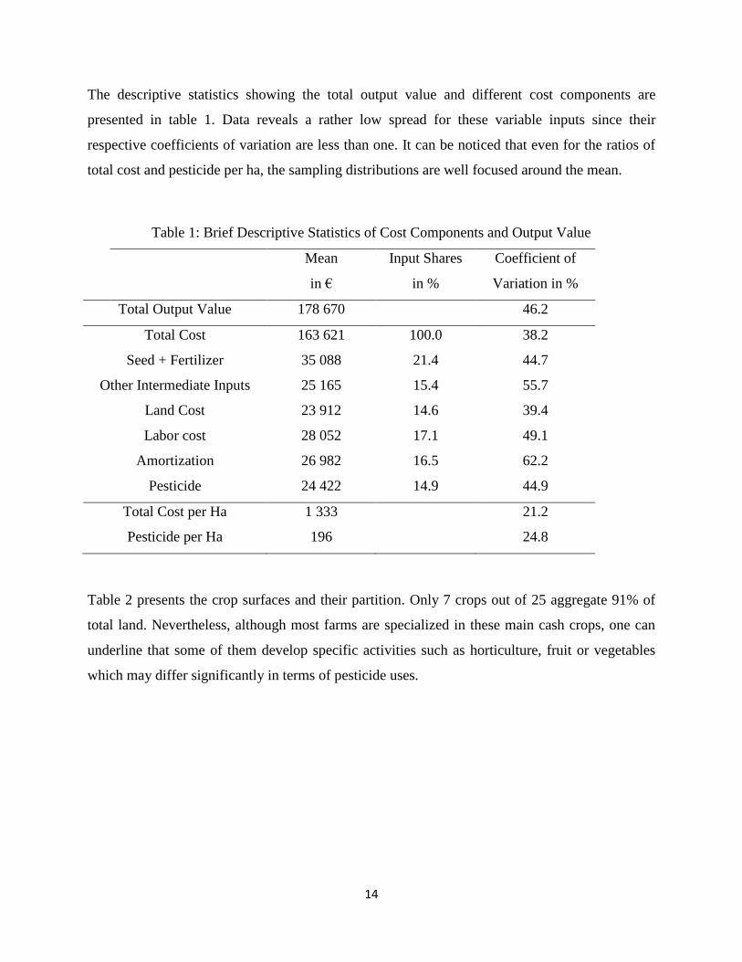
The descriptive statistics showing the total output value and different cost components are

presented in table 1. Data reveals a rather low spread for these variable inputs since their

respective coefficients of variation are less than one. It can be noticed that even for the ratios of

total cost and pesticide per ha, the sampling distributions are well focused around the mean.

Table 1: Brief Descriptive Statistics of Cost Components and Output Value

Mean

in €

Input Shares

in %

Coefficient of

Variation in %

Total Output Value 178 670 46.2

Total Cost 163 621 100.0 38.2

Seed + Fertilizer 35 088 21.4 44.7

Other Intermediate Inputs 25 165 15.4 55.7

Land Cost 23 912 14.6 39.4

Labor cost 28 052 17.1 49.1

Amortization 26 982 16.5 62.2

Pesticide 24 422 14.9 44.9

Total Cost per Ha 1 333 21.2

Pesticide per Ha 196 24.8

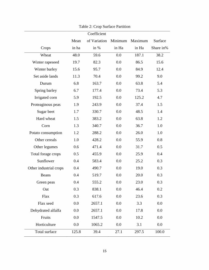
Table 2 presents the crop surfaces and their partition. Only 7 crops out of 25 aggregate 91% of

total land. Nevertheless, although most farms are specialized in these main cash crops, one can

underline that some of them develop specific activities such as horticulture, fruit or vegetables

which may differ significantly in terms of pesticide uses.

15

Table 2: Crop Surface Partition

Crops

Mean

in ha

Coefficient

of Variation

in %

Minimum

in Ha

Maximum

in Ha

Surface

Share in%

Wheat 48.0 59.6 0.0 187.1 38.2

Winter rapeseed 19.7 82.3 0.0 86.5 15.6

Winter barley 15.6 95.7 0.0 84.9 12.4

Set aside lands 11.3 70.4 0.0 99.2 9.0

Durum 6.8 163.7 0.0 63.8 5.4

Spring barley 6.7 177.4 0.0 73.4 5.3

Irrigated corn 5.9 192.5 0.0 125.2 4.7

Proteaginous peas 1.9 243.9 0.0 37.4 1.5

Sugar beet 1.7 330.7 0.0 48.5 1.4

Hard wheat 1.5 383.2 0.0 63.8 1.2

Corn 1.3 340.7 0.0 36.7 1.0

Potato consumption 1.2 288.2 0.0 26.0 1.0

Other cereals 1.0 428.2 0.0 55.9 0.8

Other legumes 0.6 471.4 0.0 31.7 0.5

Total forage crops 0.5 455.9 0.0 25.9 0.4

Sunflower 0.4 583.4 0.0 25.2 0.3

Other industrial crops 0.4 490.7 0.0 19.0 0.3

Beans 0.4 519.7 0.0 20.0 0.3

Green peas 0.4 555.2 0.0 23.0 0.3

Oat 0.3 838.1 0.0 46.4 0.2

Flax 0.3 617.6 0.0 23.6 0.3

Flax seed 0.0 2657.1 0.0 3.3 0.0

Dehydrated alfalfa 0.0 2657.1 0.0 17.8 0.0

Fruits 0.0 1547.5 0.0 10.2 0.0

Horticulture 0.0 1065.2 0.0 3.1 0.0

Total surface 125.8 39.4 27.1 297.5 100.0

16

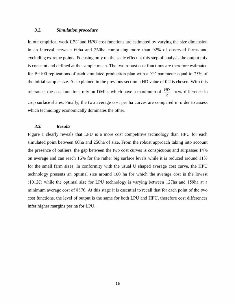
3.2. Simulation procedure

In our empirical work LPU and HPU cost functions are estimated by varying the size dimension

in an interval between 60ha and 250ha comprising more than 92% of observed farms and

excluding extreme points. Focusing only on the scale effect at this step of analysis the output mix

is constant and defined at the sample mean. The two robust cost functions are therefore estimated

for B=100 replications of each simulated production plan with a ‘G’ parameter equal to 75% of

the initial sample size. As explained in the previous section a HD value of 0.2 is chosen. With this

tolerance, the cost functions rely on DMUs which have a maximum of 10%2

HD difference in

crop surface shares. Finally, the two average cost per ha curves are compared in order to assess

which technology economically dominates the other.

3.3. Results

Figure 1 clearly reveals that LPU is a more cost competitive technology than HPU for each

simulated point between 60ha and 250ha of size. From the robust approach taking into account

the presence of outliers, the gap between the two cost curves is conspicuous and surpasses 14%

on average and can reach 16% for the rather big surface levels while it is reduced around 11%

for the small farm sizes. In conformity with the usual U shaped average cost curve, the HPU

technology presents an optimal size around 100 ha for which the average cost is the lowest

(1012€) while the optimal size for LPU technology is varying between 127ha and 159ha at a

minimum average cost of 887€. At this stage it is essential to recall that for each point of the two

cost functions, the level of output is the same for both LPU and HPU, therefore cost differences

infer higher margins per ha for LPU.

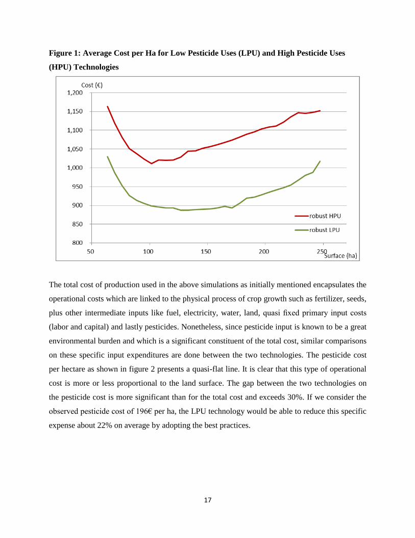
17

Figure 1: Average Cost per Ha for Low Pesticide Uses (LPU) and High Pesticide Uses

(HPU) Technologies

The total cost of production used in the above simulations as initially mentioned encapsulates the

operational costs which are linked to the physical process of crop growth such as fertilizer, seeds,

plus other intermediate inputs like fuel, electricity, water, land, quasi fixed primary input costs

(labor and capital) and lastly pesticides. Nonetheless, since pesticide input is known to be a great

environmental burden and which is a significant constituent of the total cost, similar comparisons

on these specific input expenditures are done between the two technologies. The pesticide cost

per hectare as shown in figure 2 presents a quasi-flat line. It is clear that this type of operational

cost is more or less proportional to the land surface. The gap between the two technologies on

the pesticide cost is more significant than for the total cost and exceeds 30%. If we consider the

observed pesticide cost of 196€ per ha, the LPU technology would be able to reduce this specific

expense about 22% on average by adopting the best practices.

18

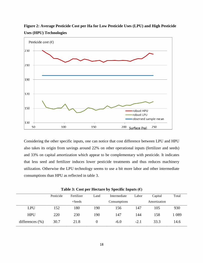
Figure 2: Average Pesticide Cost per Ha for Low Pesticide Uses (LPU) and High Pesticide

Uses (HPU) Technologies

Considering the other specific inputs, one can notice that cost difference between LPU and HPU

also takes its origin from savings around 22% on other operational inputs (fertilizer and seeds)

and 33% on capital amortization which appear to be complementary with pesticide. It indicates

that less seed and fertilizer induces lower pesticide treatments and thus reduces machinery

utilization. Otherwise the LPU technology seems to use a bit more labor and other intermediate

consumptions than HPU as reflected in table 3.

Table 3: Cost per Hectare by Specific Inputs (€)

Pesticide

Fertilizer

+Seeds

Land

Intermediate

Consumptions

Labor

Capital

Amortization

Total

LPU 152 180 190 156 147 105 930

HPU 220 230 190 147 144 158 1 089

differences (%) 30.7 21.8 0 -6.0 -2.1 33.3 14.6

19

Therefore as displayed in table 4, the cost structures of the two technologies differ but not very

significantly meaning that the adoption of LPU do not need to realize substantial substitution

effects or shift among input intensity. This result allows us to assess that the adoption of LPU

appears a relative achievable practice by all the farmers. It essentially depends on how the inputs

are effectively managed without significant reallocation among inputs.

Table 4: Cost Shares by Specific Inputs (in % of total cost)

Pesticide

Fertilizer

+ Seeds

Land

Intermediate

Consumptions

Labor

Capital

Amortization

Total

LPU 16.39 19.26 20.48 16.73 15.82 11.32 100.00

HPU 20.22 21.12 17.50 13.52 13.20 14.44 100.00

differences -3.83 -1.86 2.98 3.21 2.62 -3.12

In order to extend the previous conclusion established in the scale dimension but with respect to

the scope dimension, it is necessary to run new simulations within different crop mixes and

related input practices.

These are defined on our observed sample by a cluster analysis based on the individual crop

surface partitions. We finally concluded with five groups clearly differentiated in their output

mixes. Mix 1 is characterized by legumes, durum and irrigated corn which occupy 14%, 13%

and 10% of total surface respectively. Mix 2 is composed by farms which mainly cultivate

wheat, winter barley and rapeseed (43%, 18% and 22%). Mix 3 is made up of wheat, rapeseed

and proteaginous peas (respectively 48%, 13% and 7%). Mix 4 comprises sugar beet, spring

barley and hard wheat (14%, 11% and 19%). Finally, mix 5 is characterized by durum, irrigated

corn and potatoes (18%, 15% and 5%).

As it is observed in table 5, the crop mixes have no significant differences in terms of total land

size but three of them are characterized by a high margin level per ha thanks to some specific

remunerative crops as legumes, sugar beet, hard wheat or potatoes (mixes “legumes-durum-

corn”, “sugar beet-spring barley-hard wheat” and “durum-corn-potatoes”). The two last mixes

“wheat-winter barley-rapeseed” and “wheat-rapeseed-proteaginous peas” have an outcome of a

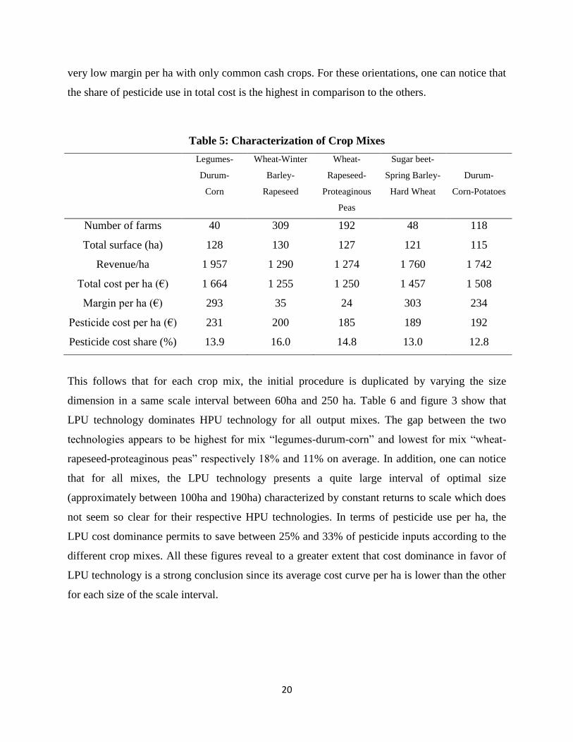
20

very low margin per ha with only common cash crops. For these orientations, one can notice that

the share of pesticide use in total cost is the highest in comparison to the others.

Table 5: Characterization of Crop Mixes

Legumes-

Durum-

Corn

Wheat-Winter

Barley-

Rapeseed

Wheat-

Rapeseed-

Proteaginous

Peas

Sugar beet-

Spring Barley-

Hard Wheat

Durum-

Corn-Potatoes

Number of farms 40 309 192 48 118

Total surface (ha) 128 130 127 121 115

Revenue/ha 1 957 1 290 1 274 1 760 1 742

Total cost per ha (€) 1 664 1 255 1 250 1 457 1 508

Margin per ha (€) 293 35 24 303 234

Pesticide cost per ha (€) 231 200 185 189 192

Pesticide cost share (%) 13.9 16.0 14.8 13.0 12.8

This follows that for each crop mix, the initial procedure is duplicated by varying the size

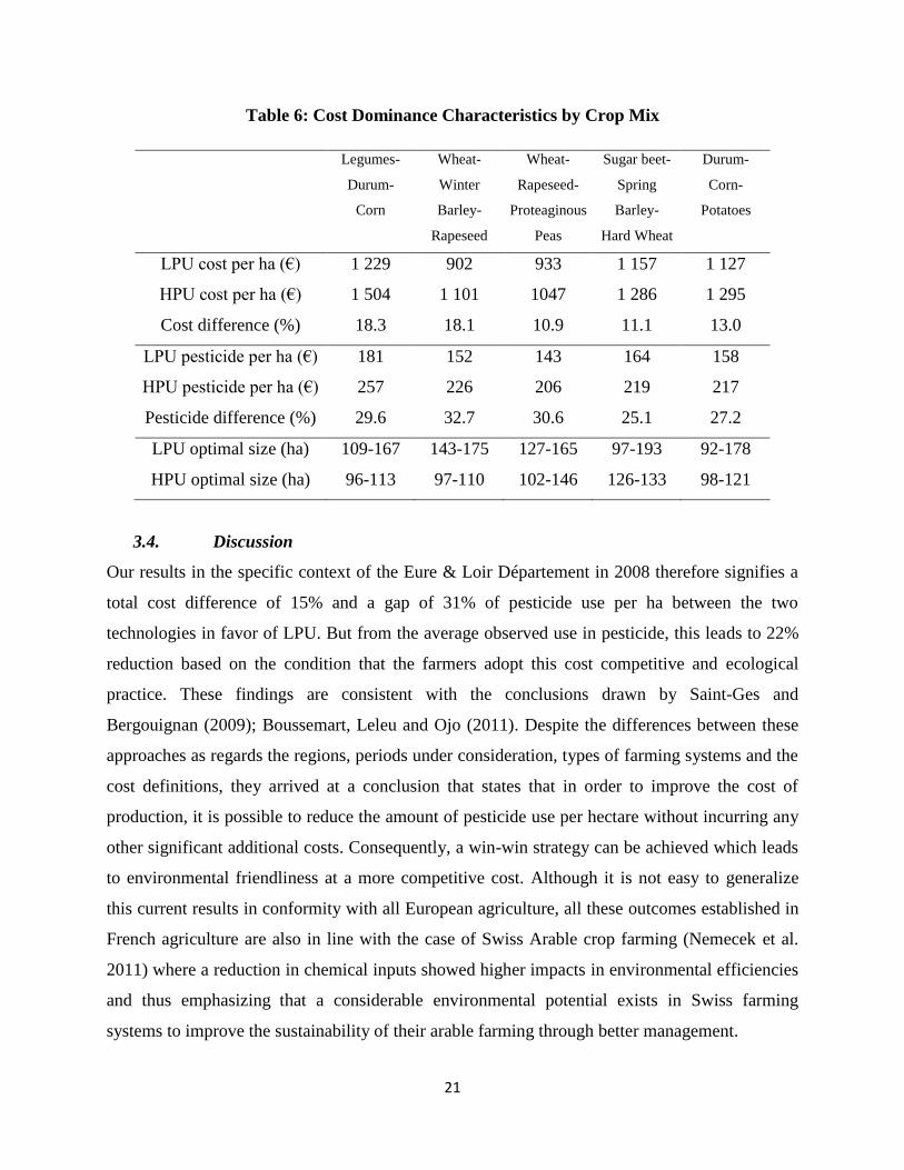
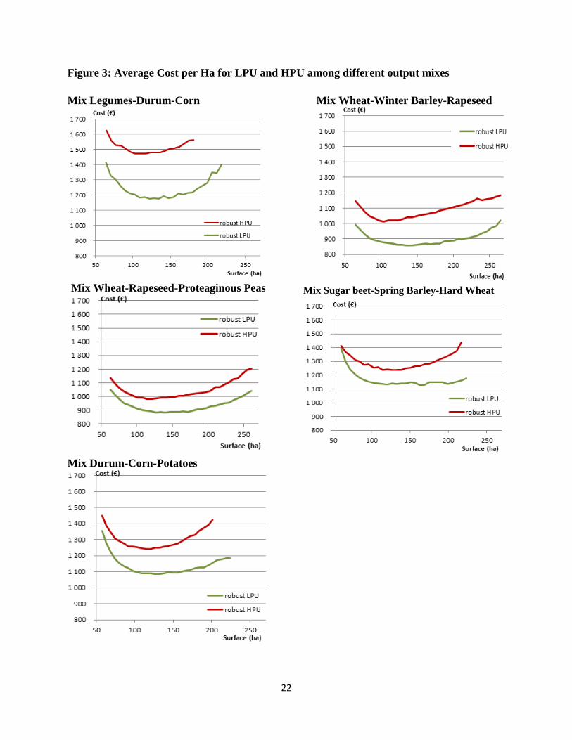
dimension in a same scale interval between 60ha and 250 ha. Table 6 and figure 3 show that

LPU technology dominates HPU technology for all output mixes. The gap between the two

technologies appears to be highest for mix “legumes-durum-corn” and lowest for mix “wheat-

rapeseed-proteaginous peas” respectively 18% and 11% on average. In addition, one can notice

that for all mixes, the LPU technology presents a quite large interval of optimal size

(approximately between 100ha and 190ha) characterized by constant returns to scale which does

not seem so clear for their respective HPU technologies. In terms of pesticide use per ha, the

LPU cost dominance permits to save between 25% and 33% of pesticide inputs according to the

different crop mixes. All these figures reveal to a greater extent that cost dominance in favor of

LPU technology is a strong conclusion since its average cost curve per ha is lower than the other

for each size of the scale interval.

21

Table 6: Cost Dominance Characteristics by Crop Mix

Legumes-

Durum-

Corn

Wheat-

Winter

Barley-

Rapeseed

Wheat-

Rapeseed-

Proteaginous

Peas

Sugar beet-

Spring

Barley-

Hard Wheat

Durum-

Corn-

Potatoes

LPU cost per ha (€) 1 229 902 933 1 157 1 127

HPU cost per ha (€) 1 504 1 101 1047 1 286 1 295

Cost difference (%) 18.3 18.1 10.9 11.1 13.0

LPU pesticide per ha (€) 181 152 143 164 158

HPU pesticide per ha (€) 257 226 206 219 217

Pesticide difference (%) 29.6 32.7 30.6 25.1 27.2

LPU optimal size (ha) 109-167 143-175 127-165 97-193 92-178

HPU optimal size (ha) 96-113 97-110 102-146 126-133 98-121

3.4. Discussion

Our results in the specific context of the Eure & Loir Département in 2008 therefore signifies a

total cost difference of 15% and a gap of 31% of pesticide use per ha between the two

technologies in favor of LPU. But from the average observed use in pesticide, this leads to 22%

reduction based on the condition that the farmers adopt this cost competitive and ecological

practice. These findings are consistent with the conclusions drawn by Saint-Ges and

Bergouignan (2009); Boussemart, Leleu and Ojo (2011). Despite the differences between these

approaches as regards the regions, periods under consideration, types of farming systems and the

cost definitions, they arrived at a conclusion that states that in order to improve the cost of

production, it is possible to reduce the amount of pesticide use per hectare without incurring any

other significant additional costs. Consequently, a win-win strategy can be achieved which leads

to environmental friendliness at a more competitive cost. Although it is not easy to generalize

this current results in conformity with all European agriculture, all these outcomes established in

French agriculture are also in line with the case of Swiss Arable crop farming (Nemecek et al.

2011) where a reduction in chemical inputs showed higher impacts in environmental efficiencies

and thus emphasizing that a considerable environmental potential exists in Swiss farming

systems to improve the sustainability of their arable farming through better management.

22

Figure 3: Average Cost per Ha for LPU and HPU among different output mixes

Mix Legumes-Durum-Corn

Mix Wheat-Rapeseed-Proteaginous Peas

Mix Durum-Corn-Potatoes

Mix Wheat-Winter Barley-Rapeseed

Mix Sugar beet-Spring Barley-Hard Wheat

23

A common, though erroneous, assumption about agricultural sustainability is that it implies a net

reduction in input use correlated to a yield reduction, thus making such systems essentially

extensive (they require more land to produce the same amount of food) which are generally

considered as less profitable by farmers. This study shows that alternative more efficient (and

thus more cost competitive) practices can lead to the same level of output per ha of surface. By

diminishing their pesticide use and also other expenses as fertilizer or capital consumption

without significant higher level of labor utilization, farmers are able to adopt more sustainable

practices characterized by a higher profitability. To this regard, recent empirical evidence shows

that successful agricultural sustainability initiatives and projects arise from shifts in the factors of

agricultural production (e.g. from use of fertilizers to nitrogen-fixing legumes; from pesticides to

emphasis on natural enemies; from ploughing to zero-tillage). A better concept than extensive is

one that centres on intensification of resources, making better use of existing resources (e.g. land,

water, biodiversity) and technologies (Buttel 2003; Tegtmeier and Duffy 2004). Thus

intensification using natural, social and human capital assets, combined with the use of best

available technologies and inputs that minimize or eliminate harm to the environment remains a

better option. Pretty, Morison and Hine (2003) examined the extent to which farmers have

improved food production with low cost, locally available and environmentally sensitive

practices and technologies and they found improvements in food production occurring through

several key practices and technologies, one of which is pest control using biodiversity services

with minimal or zero-pesticide use. Their research reveals promising advances in the adoption of

practices and technologies that are likely to be more sustainable with substantial benefits thereby

encouraging farmers to settle for practices that minimize the use of chemical inputs that can

cause harm to the environment or to the health of the farmers and consumers alike.

However, the substantial cost difference between HPU and LPU lead us to wonder why relative

high pesticide using practices are still chosen by some farmers. Risk aversion is frequently

mentioned as a justification but few researches were able to surely gauge this effect and no clear

conclusions have been established (Carpentier et al. 2005). A relevant literature debating on the

right specification of technologies incorporating pesticide as a damage-control input in a

parametric or non-parametric context (see Lichtenberg and Zilberman 1986 and Kuosmanen,

Pemsl and Wesseler 2006 among others) highlights that the usual specification of pesticide as a

24

direct input leads to overestimate its productivity and underestimate the productivity of other

inputs. Therefore agricultural policies based on these available econometric results would

promote intensive use of pesticides. Following Chambers and Lichtenberg (1994) and the initial

contribution of Lichtenberg-Zilberman, Chambers, Giannis and Vangelis (2010) conclude that

the traditional damage measure belittles the profit losses caused by pest infestations. They

highlight that when farmers are faced with pest attacks, they will take a supply-response

adjustment which boosts their income losses. This last effect is usually ignored by the traditional

pest-damage measure. Therefore pesticides seem to be less economically effective as opposed to

what other studies established.

Unfortunately, factors such as strong influence of pesticide distributors and quick results

obtained in the short term after pesticide applications could also presumably encourage farmers

to rely more on pesticide use. This high dependence on pesticides could be an indication that

farmers are less concerned about agricultural practices that are effective, inexpensive and yet

more favorable to the environment. This has been a very serious hindrance to the adoption of low

pesticide input techniques in the case of French field crop farms (Barbier et al. 2010). However,

in the case of Belgian cereal crop farmers, Vanloqueren and Baret (2008) also noted that despite

the existence of alternative technologies, the use of pesticide is still on the increase and thus

chemical inputs gradually became the main pest control strategy. They added that modern wheat

cropping practices are ‘locked-in’ to a fungicide-dependency situation which requires new

conditions (such as tougher pesticide regulations, changes in cereal prices, changing consumer

preferences, programs of pesticide reduction to evolve round greater managerial efforts and

innovative skills, etc.) to pull apart the lock-in. To this effect, they suggested that specific actions

must be undertaken to get out of this static situation.

This research therefore encourages agricultural practices that focus on the necessity to develop

technologies and practices that are environmental friendly, are accessible to and cost effective for

farmers, and lead to improvements in food productivity.

25

4. Conclusion

A competitiveness of technologies in terms of cost is established for different surface sizes, crop-

mixes and pesticide uses by exploring the cost function over its whole domain of definition.

Thus, it deals with a framework which aims at assessing the cost dominance between

technologies that favor high or low pesticide levels per ha. The authenticity of our result indicate

that low pesticide use per ha which creates environmental friendliness is more competitive in

terms of total cost in comparison to a high pesticide use which stimulates environmental burden.

While the results gotten here depend on the Eure & Loir sample and thus are not easy to

generalize in conformity with all European’s agriculture, they are totally in convergence with

previous researches using different methodological tools and other data in various European

regions.

From a methodological point of view, the originality of this study resides on several elements.

First instead of developing the usual econometric approach, cost frontier estimations are done

empirically thanks to an AAM which imposes few assumptions on the production set and does

not require any a priori specific functional form for the cost benchmark. This AAM allows the

assessment of the competiveness between two technologies characterized by different levels of

pesticide per ha. These comparisons of technologies in terms of cost are established for different

crop-mixes at several levels of size. Second the concept of Hamming Distance is endogenously

introduced in the linear programs which estimate the HPU and LPU minimal costs. This

guarantees that the optimal solution have a similar profile than the current evaluated farming

system in terms of crop surface structure. Third, in order to get round the possibility of

comparing the sensitivity of our result to the potential presence of outliers, we assume a well-

defined technology frontier by computing the expected minimal cost in a robust way, thereby

reducing the sensitivity of the cost frontier to the influence of potential outliers.

Since our results strongly show that Low Pesticide Use (LPU) dominates High Pesticide Use

(HPU) in terms of total cost, they can provide a direction for policy-makers or farmers as regards

the reduction of pesticide use in French Agriculture thus motivating environmental friendliness.

It is somehow very striking to note that practices that creates less burden to the environment and

which are simultaneously the most efficient in terms of costs are not embraced by farmers who

26

prefers the more intensive pesticide use technique to the less intensive one despite the significant

expense-gap between these two technologies, HPU and LPU respectively.

Indeed, health and environmental problems cannot be isolated from economic concerns due to

the fact that inappropriate pesticide use results not merely in yield loss but also in health

problems and possible air, soil and water pollution. The problem of farmers’ health should be an

important concern for policymakers when looking at the economic and efficiency of pesticides in

agricultural production. The conclusion from this study will inform ongoing efforts to promote

upstream policy interventions to reduce hazardous pesticide exposures for vulnerable farmers. It

is important to state that the results gotten in this paper are derived from the current technology

of farms which ensures its possibility by adopting the observed practices with low pesticide uses.

Thus, in ten years time, the aim of 50% rate of reduction may be achievable only with some

improvements in technology which will enable the farmers and the Society to opt for a win-win

strategy.

27

References

Barbier, J.M., Bonicel, L., Dubeuf, J.P., Guichard, L., Halska, J., Meynard, J.M., Schmidt, A.,

2010. Analyse des Jeux d'Acteurs. In: Ecophyto, R&D (Ed.), rapport d'expertise financé par le

Ministère de l'agriculture et de la pêche et par le Ministère de l'écologie, de l'énergie, du

développement durable et de l'aménagement du territoire, Tome VII. 74 p.

Baumol, W.J., 1958. Activity analysis in one lesson. American Economic Review 58 (5), 837–873.

BenTal, A., & Nemirovski, A., 2000. Robust solutions of linear programming problems

contaminated with uncertain data. Mathematical Programming, 88,411–421.

Boussemart, J.P., Leleu, H., Ojo, O., 2011. Could society's willingness to reduce pesticide use be

aligned with farmers' economic self-interest? Ecological Economics 70 (2011) 1797–1804.

Buttel, F.H., 2003. Internalising the societal costs of agricultural production. Plant Physiol. 133,

1656–1665.

Carpentier, A., Barbier, J.M., Bontems, P., Lacroix, A ., Laplana, R ., Lemarié, S et Turpin, N.,

2005. Aspects économiques de la régulation des pollutions par les pesticides, in: INRA (Ed.),

Pesticides, agriculture et environnement : réduire l’utilisation des pesticides et en limiter les

impacts environnementaux, Rapport de l’Expertise Collective INRA/CEMAGREF, chapitre 5.

Cazals, C., Florens, J.P., Simar, L., 2002. Nonparametric frontier estimation: a robust approach.

Journal of Econometrics 106, 1–25.

Chambers, R G, Lichtenberg, E., 1994. Simple Econometrics of Pesticide Productivity. American

Journal of Agricultural Economics 76: 407-417.

Chambers, R G, Giannis K., Vangelis T.,2010. Another Look at Pesticide productivity and pest

damage. American Journal of Agricultural Economics 1–19; doi: 10.1093/ajae/aaq066

Daraio, C., Simar, L., 2007. Conditional nonparametric frontier models for convex and non convex

technologies: a unifying approach. Journal of Productivity Analysis 28(1-2), 13-32

Dervaux, B., Leleu, H., Minvielle, E., Valdmanis, V., Aegerter, P., and Guidet, B., 2009.

Performance of French intensive care units: A directional distance function approach at the patient

level. International Journal of Production Economics 120, 585-594.

De Koeijer, T.J., Wossink, G.A.A., Struik, P.C., Renkema, J.A., 2002. Measuring agricultural

sustainability in terms of effciency. Journal of Environmental Management 66, 9–17.

Kaufmann, A., 1975. Introduction to the Theory of Fuzzy Subsets: Volume 1: Fundamental

Theoretical Elements, New York, Academic Press.

Koopmans, T.C., 1951. Activity analysis of production and allocation. Cowles Commission for

Research in Economics Monograph no. 13. John Wiley and Sons, New York.

28

Kuosmanen, T., Pemsl D., Wesseler J., 2006. Specification and estimation of production functions

involving damage control inputs: a two-stage, semiparametric approach. American Journal of

Agricultural Economics, 88(2), 499-511.

Lichtenberg, E., Zilberman, D., 1986. The Econometrics of Damage Control: Why Specification

Matters. American Journal of Agricultural Economics 68, 261–273.

McNeely, J.A., Scherr, S.J., 2001. Common ground, common future. How eco agriculture can help

feed the world and save wild biodiversity? IUCN and Future Harvest, Geneva.

Nemecek,T., Huguenin-Elie,O., Dubois, D., Gaillard,G., Schaller, B., Chervet,A.,2011. Life cycle

assessment of Swiss farming systems: II. Extensive and intensive production. Agricultural Systems

104, 233–245

Pretty, J., Ward, H., 2001. Social Capital and Environment. World Development 29(2), 209-227

Pretty, J.N., Morison, J.I.L., Hine, R.E., 2003. Reducing food poverty by increasing agricultural

sustainability in developing countries Social capital and the environment. Agriculture, Ecosystems

and Environment 95, 217–234

Robertson, G. P., Swinton, S. M., 2005. Reconciling agricultural productivity and environmental

integrity: a grand challenge for agriculture. Frontiers in Ecology and the Environment: 3(1): 38-46.

Saint-Ges, V., Be´lis-Bergouignan, M.C., 2009. Ways of reducing pesticides use in Bordeaux

Vineyards. Journal of Cleaner Production 17, 1644–1653

Shephard, R., 1953. Cost and Production Functions. Princeton University Press, New Jersey.

Simar, L., Wilson, P. W., 2008. Statistical Inference in Nonparametric Frontier Models: Recent

Developments and Perspectives in H O Fried, C A Knox-Lovell, Schmidt, The Measurement of

Productive Efficiency and Productivity Growth, Oxford: Oxford University Press

Tegtmeier, E.M., & Duffy, D.M., 2004. External Costs of Agricultural Production in the United

States. International Journal of Agricultural Sustainability. 1473-5903

Uphoff, N., (Ed.), 2002. Agroecological Innovations: Increasing Food Production with

Participatory Development. Earthscan, London

Vanloqueren, G., Baret, P.V., 2008. Why are ecological, low-input, multi-resistant wheat cultivars

slow to develop commercially? A Belgian agricultural ‘lock-in’ case study. Ecological Economics

66, 436–446.