EXPLORATORY DEVELOPMENT OF VARIM PROCESS FOR

MANUFACTURING HIGH TEMPERATURE POLYMER MATRIX

COMPOSITES

A Dissertation presented to

the Faculty of the Graduate School

University of Missouri-Columbia

In Partial Fulfillment

of the Requirements for the Degree

Doctor of Philosophy

by

AHMED KHATTAB

Dr. A. Sherif El-Gizawy, Dissertation Supervisor

JULY 2005

Dedicated to my dear wife Eman

ii

ACKNOWLEDGMENTS

All Praise is due to the almighty God; the most Gracious and the most Merciful.

I would like to thank The Boeing Company for its financial support to this project. Also,

I’d like to extend my special gratitude to Mr. Gregg Bogucki, of the Boeing Company,

for his advice about the mechanical testing procedures.

I would like to thank Dr. Donald Adams at the University of Wyoming, Dr. Rajesh

Shende at the University of Missouri-Columbia, and Dr. James Bryan at the University of

Missouri-Columbia for their advices and their useful suggestions.

Also, I extend my gratitude to the entire staff of the Department of Mechanical and

Aerospace Engineering at the University of Missouri-Columbia. The technical support of

engineering workshop’s crew, Mr. Richard Oberto, Mr. Brian Samuels, and Mr. Rix

Gish, during my experiments is highly appreciated.

I would like to acknowledge all the members of my Ph.D. committee, Dr. Uee Wan Cho,

Dr. Sanjeev Khanna, Dr. Hongbin Ma, and Dr. Hani Salim for reading the dissertation

and for their constructive remakes.

I would like to express my deepest gratitude to my advisor, Dr. Sherif El-Gizawy, for his

advice, guidance, and encouragement throughout my Ph.D. program.

iii

I would like to express my special and deepest gratitude to my parents who are pushing

me towards the success.

Last but not least, I would like to thank my dear wife, Eman, for her patience, support,

sacrifices, and encouragement during the years of my study. Also, I’d like to express my

love for my two sons, Karim and Khaled, who give me the smile and hope for the whole

life.

iv

ABSTRACT

This research focuses on an exploratory development of vacuum assisted resin infusion

molding (VARIM) process for manufacturing high temperature polymer matrix

composites for high speed civil transport. The present study involves development of a

comprehensive process virtual model and a physical model to relate the process

conditions to the evolved properties and defects in the molded composites. The virtual

model consists of three modules: the resin infusion stage; the resin cure stage; and the

cure dependant mechanical properties. The physical model investigates the feasibility of

VARIM for fabricating high temperature polymer composites and the behavior of the

process with the change in its parameters. Characterization of properties, defects, and

internal structure of produced composites is the major thrust in this study.

A virtual model for simulating the polymer flow behavior during the infusion stage was

developed and verified experimentally, with capabilities for prediction of flow pattern,

under the vacuum bagging, and evolved defects. The developed model of thermal and

cure analysis was used to get a complete temperature and cure histories of the molded

composites. The mechanical properties as functions of degree of cure and time were

determined for 5250-4-RTM resin and eight-harness carbon fiber mats.

Based on the developed virtual model and with the appropriate mold design, sound

panels, with internal voids content less than 1%, were successfully molded. Thus, the

v

VARIM process was found to be feasible for fabrication of high temperature polymer

composites. The experimental investigation shows that post cure time and maximum cure

temperature are the most significant parameters. Heating rate has a little effect on the

process. As the maximum cure temperature decreases the material strength increases.

Increasing post cure time from zero to five hours helps to increase the strength under high

humidity and high temperature condition. The study shows that, within the range used for

each parameter in the experimental design, a maximum cure temperature of 183oC, a post

cure time of 5 hours at 227°C, and a heating rate of 1.67oC/min are the optimum process

conditions for high-temperature and high-humidity applications. These curing conditions

would maximize the mechanical properties of composites molded by VARIM.

The findings of this research will help in developing a science based technology for the

VARIM process for understanding of the process behavior and the effects of various

process parameters on the properties and integrity of the produced composites.

vi

TABLE OF CONTENTS

ACKNOWLEDGMENTS ............................................................................................. ii

ABSTRACT...................................................................................................................iv

LIST OF TABLES..........................................................................................................x

LIST OF FIGURES ..................................................................................................... xii

LIST OF NOMENCLATURE.....................................................................................xvi

Chapter 1: INTRODUCTION.........................................................................................1

1.1 Problem Statement ........................................................................................1

1.2 Objectives .....................................................................................................2

Chapter 2: LITERATURE REVIEW..............................................................................4

2.1 Vacuum Assisted Resin Infusion Molding (VARIM) Process .....................4

2.2 Resin Flow Behavior.....................................................................................6

2.3 Resin Cure...................................................................................................10

Chapter 3: Investigation Approach ...............................................................................13

3.1 Process Modeling........................................................................................13

3.1.1 Virtual Flow Module....................................................................13

3.1.2 Thermal and Cure Analysis Module ............................................13

3.1.3 Cure Dependant Mechanical Properties Module .........................14

3.2 Experimental Evaluation of VARIM Process.............................................14

3.2.1 Materials ......................................................................................14

3.2.2 Fabrication Process ......................................................................15

3.2.3 Evaluation of Process-induced Properties ...................................15

vii

3.2.4 Experimental Design....................................................................16

Chapter 4: MODELING OF VARIM PROCESS.........................................................17

4.1 Virtual Flow Module...................................................................................17

4.1.1 Numerical Modeling ....................................................................18

4.1.2 Visual Presentation and Animation of the Results ......................23

4.1.3 Case Studies .................................................................................23

4.2 Thermal and Resin Cure Analysis ..............................................................29

4.3 Cure Dependant Mechanical Properties......................................................32

4.3.1 Fiber Mat Structure ......................................................................32

4.3.2 Shape Function Formulation........................................................35

4.3.3 Stiffness Matrix Formulation.......................................................38

4.4 Discussion of Cure Modeling Results.........................................................43

4.4.1 Thermal and Cure Analysis Results.............................................43

4.4.2 Composite Mechanical Properties Results...................................51

Chapter 5: EXPERIMENTAL INVESTIGATION OF VARIM PROCESS ...............60

5.1 Introduction.................................................................................................60

5.2 Materials .....................................................................................................60

5.3 Experimental Procedure..............................................................................63

5.4 Experimental Design...................................................................................67

5.5 Specimens Preparation................................................................................69

5.6 Conditioning Chamber................................................................................71

Chapter 6: CHARACTERIZATION OF PROPERTIES OF COMPOSITES

MOLDED BY VARIM...............................................................................74

viii

6.1 Introduction.................................................................................................74

6.2 Internal Structure of Molded Panels ...........................................................75

6.3 Characterization of Room-Temperature Tensile Properties .......................77

6.3.1 Test Procedure .............................................................................77

6.3.2 Data Collection ............................................................................79

6.3.3 Response Analysis .......................................................................84

6.4 Characterization of Compressive Properties of the Molded

Materials under Different Environmental Conditions ................................90

6.4.1 Room Temperature Compression Test ........................................90

6.4.1.1 Test Procedure ..............................................................90

6.4.1.2 Data Collection .............................................................91

6.4.1.3 Response Analysis ........................................................93

6.4.2 High Temperature- Dry Compression Test..................................96

6.4.2.1 Test Procedure ..............................................................96

6.4.2.2 Data Collection .............................................................98

6.4.2.3 Response Analysis ......................................................102

6.4.3 High Temperature- Wet Compression Test ...............................107

6.4.3.1 Test Procedure ............................................................107

6.4.3.2 Data Collection ...........................................................108

6.4.3.3 Response Analysis ......................................................111

6.5 Discussion of Experimental Results .........................................................114

6.6 Empirical Model of VARIM Process .......................................................119

6.7 Comparison of Properties of Composites Produced by ............................129

ix

VARIM and other Molding Techniques

Chapter 7: CONCLUSIONS AND RECOMMENDATIONS ...................................131

7.1 Introduction...............................................................................................131

7.2 Conclusions...............................................................................................132

7.3 Recommendations.....................................................................................134

APPENDIX A.............................................................................................................135

APPENDIX B .............................................................................................................141

APPENDIX C .............................................................................................................144

APPENDIX D.............................................................................................................150

REFERENCES ...........................................................................................................153

VITA...........................................................................................................................159

x

LIST OF TABLES

Table Page 4.1 Kinetic parameters for 5250-4-RTM resin ........................................................ 43 4.2 Some case studies used to produce composite panel by VARIM ..................... 44 4.3 Elastic properties of the carbon fiber AS4 and 5250-4-RTM resin................... 51 4.4 Cure dependent properties for carbon fiber/5250-4-RTM resin........................ 57 5.1 Control factor levels corresponding to their coded levels ................................. 68 5.2 Three parameter central composite design ........................................................ 68 6.1 Percentage of voids obtained by image analysis for some samples

produced by VARIM ......................................................................................... 76 6.2 Process parameters effect on ultimate tensile strength for each case ................ 82 6.3 Process parameters effect on tensile modulus for each case ............................. 83 6.4 Analysis of variance for ultimate tensile strength ............................................. 87 6.5 Analysis of variance for tensile modulus at room temperature ......................... 89 6.6 Process parameters effect on compressive strength at room temperature ......... 92 6.7 Analysis of variance for max compressive strength at room temperature......... 95 6.8 Process parameters effect on the compressive strength for high temp-dry ..... 100 6.9 Process parameters effect on the compressive modulus for each case............ 101 6.10 Analysis of variance for compressive strength at high temperature-dry ......... 104 6.11 Analysis of variance for compressive modulus at high temperature-dry ........ 107 6.12 Percentage of weight gain after condoning and at time of test........................ 108 6.13 Process parameters effect on the compressive strength for high temp-wet..... 110

xi

6.14 Analysis of variance for compressive strength at high temperature-wet......... 113 6.15 Analysis of variance for compressive strength at high temperature-wet......... 120 6.16 Predicted strength and corresponding percent error of model for each case... 121 6.17 Optimum process parameters and the model predicted response.................... 122 6.18 Response polynomial coefficients for maximum compressive strength ......... 123 6.19 Predicted strength and corresponding percent error of model for each case... 124 6.20 Optimum process parameters and the model predicted response.................... 125 6.21 Response polynomial coefficients for maximum compressive strength ......... 126 6.22 Predicted strength and corresponding percent error of model for each case... 127 6.23 Optimum process parameters and the model predicted response.................... 128

xii

LIST OF FIGURES

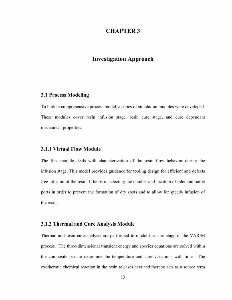
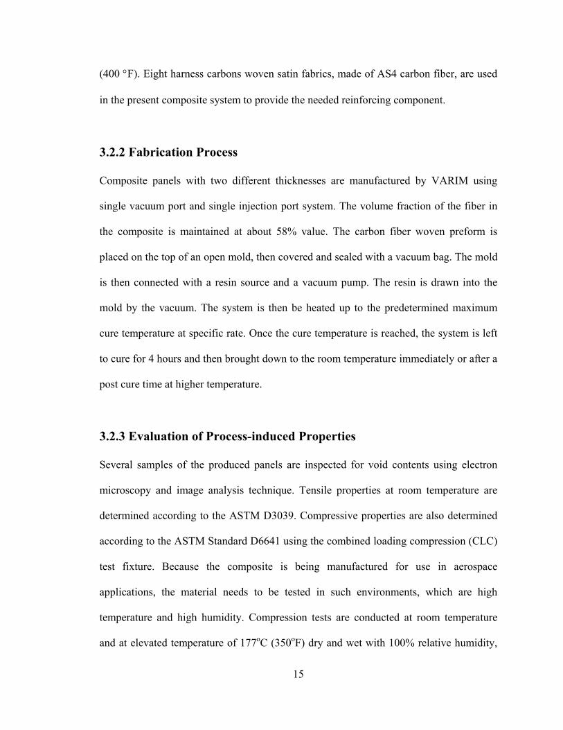
Figure Page 4.1 Schematic diagram of the experimental setup................................................... 20 4.2 Resin flow front during infusion stage .............................................................. 26 4.3 The thick white line represents the actual resin flow front................................ 26 4.4 Resin flow front with the effect of race-tracking during resin infusion ............ 27 4.5 Race-tracking effect, (a) the flow front during infusion and (b) macro-void

due to race-tracking effect at the end of mold filling ........................................ 27 4.6 Marc-void due to race-tracking effect, (a) the simulation result and (b) the

actual part (the thick white line surrounds an air void) ..................................... 28 4.7 Resin flow front during infusion stage, a) experimental, b) simulation

results, c) actual flow front near the end of infusion stage................................ 28 4.8 Schematic of a top view of eight-harness carbon fiber mat .............................. 33 4.9 Geometry of a cross section of eight-harness carbon fiber mat, (a) a CAD

drawing (b) a picture obtained by optical microscope for sample produced by VARIM......................................................................................................... 34

4.10 Geometry of eight-harness carbon fiber mat. Each section represents a cross

section of the mat along the y-direction ............................................................ 34 4.11 Geometry of a cross section of eight-harness carbon fiber mat......................... 35 4.12 Geometrical relation between the fill yarn and the warp yarn of 8H fiber

mat ..................................................................................................................... 35 4.13 Variation of resin elastic modulus and Poisson’s ratio with cure...................... 41 4.14 Cure and temperature histories for case 1 ......................................................... 46 4.15 Distribution of degree of cure through the panel thickness along the length .... 47 4.16 Distribution of degree of cure through the panel thickness along the width..... 47 4.17 Distribution of temperature through the panel thickness along the length........ 48

xiii

4.18 Distribution of degree of cure through the panel thickness along the length .... 48 4.19 Cure and temperature histories for case 2 ......................................................... 49 4.20 Cure history comparison for cases 1and 2......................................................... 49 4.21 Cure history comparison for cases 3and 4......................................................... 50 4.22 Distribution of Young’s modulus for section A-A at the end of cure cycle...... 52 4.23 Distribution of Young’s modulus at an area with fiber undulation................... 53 4.24 Average of Young’s modulus through the thickness and along the length ....... 54 4.25 Average of Young’s modulus through the thickness and along the length ....... 54 4.26 Average of Young’s modulus through the thickness and along the length

for the 8 sections of the unit cell of a one-layer laminate.................................. 55 4.27 A laminate with six layers of carbon fiber randomly distributed ...................... 56 4.28 Average of Young’s modulus through the thickness and along the length

for the 8 sections of the unit cell of a six-layer laminate................................... 56 4.29 Variation of Young’s modulus with resin degree of cure ................................. 57 4.30 Variation of extensional stiffness with resin degree of cure ............................. 58 4.31 Variation of bending-extension stiffness with resin degree of cure .................. 59 4.32 Variation of bending stiffness with resin degree of cure................................... 59 5.1 Chemical structures of 5250-4 RTM resin components, taken from ................ 62 5.2 Chemical structure of the combined 3-component 5250-4 RTM resin ............. 62 5.3 Schematic diagram of the experimental setup................................................... 65 5.4 VARIM experimental setup-carbon fiber at the top of the mold ...................... 66 5.5 VARIM experimental setup-vacuum bag covers the mold ............................... 66 5.6 VARIM experimental setup............................................................................... 66 5.7 Machining of composite specimen using a special fixture................................ 69

xiv

5.8 Lateral lines being cut in the composite panel .................................................. 70 5.9 Machining of the edges of carbon fiber composite sample ............................... 70 5.10 Environmentally controlled chamber ................................................................ 72 5.11 Setup of conditioning chamber.......................................................................... 73 5.12 Composite specimens loaded in the conditioning chamber............................... 73 6.1 Scanning electron micrograph of composite material produced by VARIM.... 75 6.2 Image analysis micrograph report showing the low micro-voids contents

(average 0.25%)................................................................................................. 76 6.3 Dimensions in millimeter of coupon used in tensile test................................... 78 6.4 Tension test setup for composite sample........................................................... 78 6.5 Stress-strain curve of tensile test for one of the cases ....................................... 79 6.6 Scatter plot of tensile strength for each case shown in table 6-2....................... 82 6.7 Scatter plot of tensile modulus for each case shown in table 6-3...................... 83 6.8 Average main effect of post cure time on ultimate tensile strength .................. 84 6.9 Average main effect of max cure temperature on ultimate tensile strength ...... 85 6.10 Average main effect of heating rate on ultimate tensile strength ...................... 85 6.11 Average main effect of heating rate on tensile modulus ................................... 88 6.12 Average main effect of post cure time on tensile modulus ............................... 88 6.13 Average main effect of max cure temperature on tensile modulus ................... 89 6.14 Combined loading compressive test fixture ...................................................... 91 6.15 Scatter plot of tensile modulus for each case shown in table 6-6...................... 92 6.16 Average main effect of post cure time on compressive strength....................... 93 6.17 Average main effect of heating rate on compressive strength........................... 94 6.18 Average main effect of max cure temperature on compressive strength .......... 94

xv

6.19 Combined load compression (CLC) modified fixture....................................... 96 6.20 One half of the CLC modified fixture showing the heating system.................. 97 6.21 The specimen with the strain gage used in the compression test ...................... 98 6.22 Stress-strain curve for compression test of one of the cases ............................. 99 6.23 Scatter plot of compressive modulus for each case shown in table 6-8 .......... 100 6.24 Scatter plot of compressive modulus for each case shown in table 6-9 .......... 101 6.25 Average main effect of post cure time on compressive strength..................... 102 6.26 Average main effect of max cure temperature on compressive strength ........ 103 6.27 Average main effect of heating rate on compressive strength......................... 103 6.28 Average main effect of max cure temperature on compressive modulus........ 105 6.29 Average main effect of post cure time on compressive modulus.................... 105 6.30 Average main effect of heating rate on compressive modulus........................ 106 6.31 Scatter plot of compressive modulus for each case shown in table 6-13 ........ 110 6.32 Average main effect of post cure time on compressive strength..................... 111 6.33 Average main effect of max cure temperature on compressive strength ........ 112 6.34 Average main effect of heating rate on compressive strength......................... 112 6.35 Comparison between the measured and the predicted tensile strength ........... 121 6.36 Predicted tensile strength versus measured tensile strength............................ 122 6.37 Comparison between the measured and the predicted compressive strength.. 124 6.38 Predicted compressive strength versus measured compressive strength......... 125 6.39 Comparison between the measured and the predicted compressive strength.. 127 6.40 Predicted compressive strength versus measured compressive strength......... 128 6.41 Comparison between the VARIM, RTM and prepreg molding technique...... 130

xvi

LIST OF NOMENCLATURE A1, 2 : Arrhenius constants (1/s)

Aij : Extensional stiffnesses (N/m)

Bij : Bending-extension coupling stiffnesses (Pa m2)

CA : Local concentration of the uncured resin

CI : Initial concentration of uncured resin

pc : Specific heat (J/kg K)

pfc : Specific heat of fiber (J/kg K)

prc : Specific heat of resin (J/kg K)

Dij : Bending stiffnesses (Pa m2)

Em : Tensile modulus of matrix (GPa)

Ef : Tensile modulus of fiber (GPa)

Ek : Activation energy (J/mole)

Gm : Shear modulus of matrix (GPa)

Gf : Shear modulus of fiber (GPa)

H : Height (m)

th : Thickness of matrix top layer (m)

zh : Yarn thickness (m)

Keff : Effective permeability (m2)

Krace : Equivalent race tracking permeability (m2)

xvii

K1, 2 : Reaction rate constants

k : Thermal conductivity (W/m K)

fk : Thermal conductivity of fiber (W/m K)

rk : Thermal conductivity of resin (W/m K)

n : Order of the reaction

P : Pressure (N/m2)

R : Universal gas constant

Ra : Reaction rate (1/s)

Sa : Source term due to chemical reaction (W/m3)

t : Time (s)

ui : Velocity component of resin in xi direction (m/s)

fV : Fiber volume fraction

W : Width (m)

fw : Weight fraction of fiber

rw : Weight fraction of resin respectively

gx : Offset distance of the warp yarn from zero coordinate (m)

oz : Center line of fill yarn (m)

uz : Upper boundary of the fill yarn (m)

lz : Lower boundary of the fill yarn (m)

a : Wavelength of a yarn (m)

tz : Boundary of elliptical shape of warp yarn (m)

airε : Volume fraction of air

xviii

sinreε : Volume fraction of resin

airρ : Density of air (kg/m3)

sinreρ : Density of resin (kg/m3)

airµ : Viscosity of air (Pa s)

sinreµ : Viscosity of resin (Pa s)

Ψ : Degree of cure

∆H : Heat of reaction (J/kg)

ρ : Density (kg/m3)

fρ : Density of fiber (kg/m3)

rρ : Density resin (kg/m3)

θ : Angle between fiber direction and x-axis

mν : Poisson’s ratio of matrix

fν : Poisson’s ratio of fiber

1

CHAPTER 1

INTODUCTION

1.1 Problem Statement

The Vacuum Assisted Resin Infusion Molding (VARIM) is a manufacturing process for

composite structures [1-3]. In this process, the reinforcement, which is usually composed

of several layers of woven fiber mats, is placed in an open mold and a plastic vacuum bag

is placed on the top of the mold. The mold is connected with a resin source and a vacuum

pump. As the vacuum is drawn through the mold, the liquid resin infuses into the

reinforcing fiber mats. Curing and de-molding steps to finish the product follow this. In

the vacuum assisted resin infusion molding (VARIM) process a highly permeable

distribution fabric, known as distribution medium is used in order to accelerate the

infusion process and to enhance the liquid resin penetration in the thickness direction [4].

VARIM has become very attractive fabrication technology in recent years because of its

low cost tooling and scalability to very large structures. It minimizes the void contents

inside the molded composites, reduces VOC emissions, and results in less scrap than

other molding techniques [5, 6]. Nevertheless, VARIM has been used primarily with

resin systems that cure at room temperature such as vinyl ester. High temperature

polymer matrix composites for high performance applications that require cure at high

temperature are currently produced by the autoclave/prepreg molding technique. This

2

process is not cost effective and limited to small size structures. The potentials of

VARIM for fabricating high temperature polymer composite structures with properties

and quality match those of the autoclave/prepreg molded ones are widely unexplored.

1.2 Objectives

This research focuses on an exploratory development of VARIM process for

manufacturing high temperature polymer matrix composites. It addresses material

characterization, process verification and identification of transition pathways.

This work aims at developing a science-based technology for VARIM of high

temperature polymer matrix composites for the understanding of the process behavior

and the effects of various process parameters on the properties and integrity of the

produced composites. Some important issues remain to be explored before high

temperature VARIM can be widely used for variety of applications. Process–induced

damage in the form of voids, and macro-voids (dry spots) developed during processing

are reported as the most significant problems in liquid composite molding particularly for

materials that cure at high temperature [6-9]. These process-induced defects can cause

significant changes in the geometry and serious degradation of the mechanical properties

of the molded structure. The absence of a knowledge base involving the processing-

material-performance relationship for VARIM of high temperature polymer composites;

delays the introduction of such strategic materials to the next generation high speed and

light weight transports.

3

The numerical-experimental investigation will provide the capability for robust process

and tooling design, prediction and characterization of process-induced damage and

properties of high temperature polymer composites produced by VARIM. The following

are the specific objectives of this study:

• Development of a predictive model based on control volume technique in order to

characterize the polymer flow behavior in VARIM of composite structures.

• Development of a 3D finite difference model to determine composite thermal and

cure histories during the cure cycle

• Determination of cure-dependent mechanical properties for eight-harness carbon

/5250-4 resin system.

• Perform parametric tests using the design of experiments method on VARIM of

the eight-harness carbon /5250-4 resin system, in order to investigate the effects

of process parameters on the quality of the produced structures and to develop an

empirical relationship between process parameters and the evolved properties.

4

CHAPTER 2

LITERATURE REVIEW

2.1 Vacuum Assisted Resin Infusion Molding (VARIM) Process

High temperature matrix composites are needed for high speed civil transport and

advanced tactical fighters. Typical airframe materials for such applications must endure

120,000 hours at temperatures approaching 180oC (350oF) [10]. High temperature matrix

composites are currently produced by autoclave/prepreg molding technique. This process

is not cost effective and limited to small size structures. Uneven distribution of pressure

and temperature during consolidation and curing of large parts are typical problems of the

autoclave technique. Such problems can cause an uneven cure, warpage, voids, and low

fiber volume fraction [7, 11]. Conventional resin transfer molding (RTM) is also used for

manufacturing large composite parts using high temperature polymers. The low volume

fraction of fibers (maximum value of 40%) that can be used in the process and the high

concentration of voids (greater than 1%) in the molded composites limit RTM to the

production of secondary structure members and light load applications. [12]. VARIM

offers a manufacturing process of composite materials, which are more affordable than

those from autoclave techniques. The application of VARIM manufacturing of the

Lockheed Martin Joint Air-to-Surface Standoff Missile (JASSM) has showed cost

savings over the autoclave process [13]. Also composite materials produced by vacuum

5

assisted show superior mechanical properties over those produced by RTM due to the

high fiber volume fraction (up 60%).

Until recently, VARIM had not been used for high temperature polymer matrix

composites because of the limitation of resins availability with low melt viscosity and log

melt stability. Fortunately, the Cycom 5250-4-RTM resin system, introduced by Cytec

Engineered Materials, satisfies these needs. This resin reaches very low viscosity during

transfer and maintains a low viscosity for several hours. Laminates fabricated from this

resin are capable of service temperatures up to 204oC (400oF) [14]. Higher processing

temperatures are required to obtain composite materials for high temperature use. The

high processing temperature in VARIM presents a challenge for bagging and sealing

materials. Criss and Koon [15] used phenylethynyl terminated imides (PETI), which is a

high temperature polymer, to fabricate composites using VARIM. The quality of the

laminates was determined based on voids contents and mechanical properties. In this

work, panels with 4% porosity showed mechanical performance suitable for structural

applications. More work is needed to be done to refine the process conditions to reduce

porosity and to improve properties.

A comprehensive review for the historical development of vacuum assisted resin infusion

(VARI) was introduced by Williams et al. [16]. The study reviewed the progress of VARI

from its first development by Macro [17] to the Seemann composites resin infusion

manufacturing process (SCRIMP) [18]. The review showed that the development of

VARI process has been slow (compared to RTM). Generally, there is little information

6

available about the properties and process-induced defects of high temperature polymer

composites structures produced by VARIM processes. A better understanding of evolved

mechanical properties and the significance of process-induced damage in these processes

are required before the introduction of new composites systems in the design of large

structures for high performance applications.

2.2 Resin Flow Behavior

The proper infusion of the reinforcing fibers with the liquid polymer requires proper

positioning of the inlets and outlets, close monitoring of mold temperature and vacuum

pressure, and selection of optimum resin flow rate into the mold. Proper positioning of

the filling port helps in eliminating the formation of voids and hence in generating

composites parts with good quality. Trochu and Gauvin [19] employed a boundary-fitted

finite difference method to model a two-dimensional RTM process. Their model is

capable of obtaining the resin front and pressure distribution within the mold. They also

discussed the limitations of finite difference method in modeling this process. They

performed experiments and compared the experimental and numerical results. These

investigators noticed the difference between numerical simulations and experimental

observations of the resin front positions. They suggested that this difference is due to

edge effects. However, they claimed that these edge effects could not be easily modeled

numerically.

Later on, A. Hammami [20], and S.G. Advani [7] presented an analysis to describe the

race-tracking (edge effect) using appropriate flow equation in an open channel (mold

7

edge) and Darcy’s law in the porous medium. Then an equivalent permeability can be

computed for the channel. Pillai and Advani [21] simulated the unsaturated flow

encountered in woven fiber mats used in RTM, using a finite element method. The resin

flow inside the mold is modeled as a flow through porous media. They presented results

on simple flow at constant injection pressure in 1-D flow and constant flow rate radial

injection flow. Diallo et al [22] developed a similar model. They addressed the effects of

variation in the through thickness and in-plane porosity and permeability. Colestenian

and El-Gizawy [23] performed both physical and numerical modeling using a finite

element technique on the RTM process. The effects of injection pressure, resin viscosity,

type of reinforcement, and mold geometry on mold filling times were investigated.

Comparison between the experimental and numerical results of the resin front position

indicated the importance of edge effects (race-tracking) in resin flow behavior in small

cavities with larger boundary areas. Increasing the permeability at the edge region in the

numerical model allowed for reasonable agreement between the numerical and the

physical observations of the resin flow front position and mold filling time.

El-Gizawy and Kuan [24] used a control volume technique based on the finite difference

method to characterize the polymer flow behavior in resin transfer molding of woven

fiber composite structures. In their model, transient terms are considered in order to

accurately describe the behavior of the polymer front during the injection stage. An

analytical model [25] was introduced in order to investigate the role of vacuum pressure

and port locations on flow front control for liquid molding processes. The parametric

studies used in this investigation resulted in a relationship that captures the important

8

physics. This relationship can be used for flow front control and hence avoiding

incomplete filling problems. In another study [26], a model was developed to analyze

resin flow through a deformable fiber preform in VARIM process. The force balance

between the resin and the fiber preform is used to account for the swelling of the preform

inside the flexible vacuum bag. The application of the developed model was

demonstrated using a large panel with complex geometry.

A recent study [27] introduced a new approach to get an optimum arrangement of gates

and vents locations for RTM process design based on the mesh distance concept. In order

to reduce the computational time for mold filling simulation, the proposed process used a

genetic algorithm, instead of numerical simulation, to determine the gate and vent

locations. The model was tested on several cases obtained from literature. The model was

found effective, but further work needs to be done to include important process

parameters, such as permeability and part thickness. Another study was conducted by B.

Kim et al. [28], to determine the optimum gate location based on numerical simulation

and optimization process using a genetic algorithm. The results were compared to

experiments for several cases with different permeability and different part thickness. The

results showed a good agreement between the algorithm and the experimental work. A.

Gokce el al. [29] used branch and bound search to find the optimum gate locations in

liquid composite molding process. The study is conducted in a virtual optimization and a

control environment created by the integration of simulation software and math software.

The method was compared with exhaustive search and genetic algorithms. The results

were very promising for the case studies conducted for single gate optimization in RTM.

9

More research is needed to be conducted for multiple gate optimization problems. B.

Minaie et al. [30] presented an inverse methodology that directly calculates the optimum

inlet conditions in order to achieve a desired filling pattern such that the last point to fill

(LPF) location coincides with the preset exit vent location that is specified during RTM

process design. The proposed inverse algorithm was successfully applied to a rectangular

mold with two inlet gates in order to determine the location of vent. The algorithm needs

to be validated with different mold shapes, especially more complex shapes.

Choi and Dharan [31], addressed a novel process to over come the decay in the pressure

with distance from the inlet port in RTM. They proposed a process named articulated

RTM in which the mold is designed to be articulated such that the mechanical action of

the articulated segments create high local pressure that facilitate the fluid flow and hence

reduce the mold filling time with less void generation. Smaller segments and a large

number of segments result in shorter mold fill times [32]. However, this approach is very

limited to small parts due to the tooling complexity and the high cost. P. Luca et al. [33]

gave an overview of the liquid composite molding (LCM) process modeling issues with a

review of preforming simulation in RTM. This study emphasized that the critical material

parameter that drives the resin flow in the RTM simulation is the permeability.

Joubaud and Trochu [34] presented an approach to simulate vacuum assisted resin

infusion based on an equivalent flexible mold permeability using an existing RTM

software. The study showed that the porosity of the reinforcement and hence the

permeability depend on the vacuum level under the flexible plastic bag. Then the

10

permeability measured in a stiff mold cannot be used to simulate the VARIM process. A

modified value of permeability, called flexible mold permeability, was either measured

experimentally or derived from the compressibility and permeability of the fabric. The

comparison between an experimental case study and the simulation results showed a

fairly good agreement. The simulation did not take into consideration the influence of the

flow-enhancing layer, the infusion mesh, or the peel ply, which need to be investigated.

Another experimental study was conducted by A. Hammami [35], to investigate the main

factor affecting the permeability measurement in the VARIM process. The study

investigated experimentally the effect of a flow enhancement layer and the infusion

mesh. However, the use of the infusion mesh helped to reduce the filling time. The

findings showed the need for additional experimental work, and also, for a simulation

model covering the whole parameters which will help in reducing the experimental work

needed.

2.3 Resin Cure

A series of analysis on modeling the effect of cure on residual stress development in

laminate composites was performed by White and Hahn [36-38]. Their two-dimensional

model [36] was developed to predict cure and residual stress in an automotive process.

They used cure dependent mechanical properties in their model. In a subsequent work,

White and Hann [37, 38] presented experimental results on residual stress formation in an

autoclave or hot press processing. Golestanian and El-Gizawy [39] presented results on

cure-dependent properties of resin transfer molded thin composites with woven fiber

mats. In this study, resin properties are assumed to change from viscoelastic liquid to

11

properties of the solid as the part cures. Osswald et al. [40] performed analysis on

shrinking and warpage of compression-molded fiber reinforced composite parts. Their

research concentrated on numerical simulation and experimental investigation of

shrinkage and warpage in thin compression molded parts. Their numerical model

incorporated cure-dependent mechanical properties of the composite. They considered

the composite at a macroscopic scale and did not differentiate between the fiber and resin

rich regions.

Bogetti and Gillespie [41] investigated thickness and autoclave temperature effects on

formation of residual stresses in laminate composites. Their results indicated complex

thermal and cure gradients in thick composite laminates. The effects of these gradients on

process induced residual stresses were shown to be important. Tseng and Osswald [42]

performed analysis on thermo-mechanical behavior of compression molded composite

parts. They used a coupled temperature and stress simulation program to determine

residual stress build up during curing of the part. They studied the effect of fiber content,

part thickness, unsymmetrical curing and flow-induced fiber orientation on the shrinkage

and warpage of the molded parts. Their results indicated a significant effect of warpage

on fiber orientation. Their analysis was on compression molding of random fiber

composites, since they considered thin composite parts, their thermal analysis was one-

dimensional. They also neglected coupling between stretching and bending of the

composite laminate. In an effort to simulate the entire VARIM process, a three-

dimensional model was developed [43]. It constitutes modules for describing the resin

flow, heat transfer, preform compaction, cure kinetics, and residual stresses during

12

infiltration and cure. The published work shows only the experimental verification of the

resin flow module. They addressed VARIM process for resins that cure at room

temperature (vinyl ester). Y. Kim and I. Daniel [44], conducted an experimental study to

investigate the cure cycle effects on residual stress, and residual strain on new material

fabricated by RTM process. Three different cure cycles with different peak temperature

and different heat rates were used. The study showed that the residual stress developed at

high cure temperature was lower than that developed at a lower cure temperature due to

the constraint induced strain. The effect of different heat up rates was not that clear.

The literature review shows that a large portion of the published work on process

modeling for woven fiber/high temperature polymer composites deals primarily with the

conventional RTM process. Nevertheless, these findings and results could also help in the

development of the science-based technology for VARIM processes using high

temperature polymers. This work will address the gaps in the current literature and

develop a more generic model to simulate the VARIM process. This comprehensive

research covers both the infusion (polymer flow) stage and the cure stage. The numerical-

experimental investigation will provide a capability for robust process and tooling design,

prediction, and characterization of process-induced properties of high temperature

polymer composites produced by VARIM.

13

CHAPTER 3

Investigation Approach

3.1 Process Modeling

To build a comprehensive process model, a series of simulation modules were developed.

These modules cover resin infusion stage, resin cure stage, and cure dependant

mechanical properties.

3.1.1 Virtual Flow Module

The first module deals with characterization of the resin flow behavior during the

infusion stage. This model provides guidance for tooling design for efficient and defects

free infusion of the resin. It helps in selecting the number and location of inlet and outlet

ports in order to prevent the formation of dry spots and to allow for speedy infusion of

the resin.

3.1.2 Thermal and Cure Analysis Module

Thermal and resin cure analysis are performed to model the cure stage of the VARIM

process. The three-dimensional transient energy and species equations are solved within

the composite part to determine the temperature and cure variations with time. The

exothermic chemical reaction in the resin releases heat and thereby acts as a source term

14

in the energy equation. Thus the energy and species equations become coupled and need

to be solved simultaneously. The degree of cure as a function of time and temperature are

determined.

3.1.3 Cure Dependant Mechanical Properties Module

Once the composite degree of cure is known with time, the stiffness matrices could be

determined as functions of degree of cure and time. Classical Laminate Theory (CLT) is

assumed to be applicable to the infinitesimal regions of the composite unit cell. Cure

dependent mechanical properties of composite parts with eight-harness fiber mats are

determined. Resin properties are assumed to change from that of a liquid to properties of

a solid as the part cures. This module takes into account the fiber continuity and

undulation. Resin rich areas between fiber bundles and the fraction of resin within the

fiber bundles are taken into account too. The components of the stiffness, coupling

stiffness, and bending stiffness matrices are modeled for the investigated systems. For

the fill and warp yarns, the changes in fiber orientation due to fiber undulation are taken

into account.

3.2 Experimental Evaluation of VARIM Process

3.2.1 Materials

The high temperature resin used is CYCOM 5250-4-RTM produced by CYTEC

Engineered Materials in California. It is a one-part homogenous Bismaleimide (BMI)

resin with some additives to improve toughness [45]. This polymer was developed for use

in high performance structural composites requiring high temperature use up to 204 ºC

15

(400 °F). Eight harness carbons woven satin fabrics, made of AS4 carbon fiber, are used

in the present composite system to provide the needed reinforcing component.

3.2.2 Fabrication Process

Composite panels with two different thicknesses are manufactured by VARIM using

single vacuum port and single injection port system. The volume fraction of the fiber in

the composite is maintained at about 58% value. The carbon fiber woven preform is

placed on the top of an open mold, then covered and sealed with a vacuum bag. The mold

is then connected with a resin source and a vacuum pump. The resin is drawn into the

mold by the vacuum. The system is then be heated up to the predetermined maximum

cure temperature at specific rate. Once the cure temperature is reached, the system is left

to cure for 4 hours and then brought down to the room temperature immediately or after a

post cure time at higher temperature.

3.2.3 Evaluation of Process-induced Properties

Several samples of the produced panels are inspected for void contents using electron

microscopy and image analysis technique. Tensile properties at room temperature are

determined according to the ASTM D3039. Compressive properties are also determined

according to the ASTM Standard D6641 using the combined loading compression (CLC)

test fixture. Because the composite is being manufactured for use in aerospace

applications, the material needs to be tested in such environments, which are high

temperature and high humidity. Compression tests are conducted at room temperature

and at elevated temperature of 177oC (350oF) dry and wet with 100% relative humidity,

16

to determine the response of these molded composite materials when stressed in these

environments.

3.2.4 Experimental Design

An experimental plan has been designed to study the effects of process variables. A

partial factorial design of experiments involves three major parameters is conducted on

VARIM for high temperature resin composites. The process variables in the design

include: maximum curing temperature, heating rate during the cure stage, and post cure

time at higher temperature after curing. In order to obtain generality and precision for the

developed experimental database for the process, the experiments needed to generate the

required data must be conducted in a systematic and organized way. The unifying feature

of statistically designed experiments is that all factors of interest are varied

simultaneously. In this way, the maximum amount of information can be extracted with

a minimum number of experiments. The response surface methodology (RMS) [46] is

useful for cases where the responses of interest are influenced by several process factors

and where the main objective is to optimize these responses.

17

CHAPTER 4

MODELING OF VARIM PROCESS

4.1 Virtual Flow Module

A virtual flow model for process design in vacuum assisted resin infusion operations is

developed. It uses a control volume technique based on finite difference method to

characterize flow behavior during resin infusion in molding woven fiber composite

structures. In order to enhance the visual capability of the developed virtual model, a

geometric reconstruction scheme is used to present the resin flow front at fixed time

increment. The Graphic Interchange Format (GIF) is used to combine images into a

single file to create animation. This model provides capabilities for prediction of flow

pattern and evolved defects. Several case studies were conducted to evaluate the

effectiveness of the developed model.

Numerical simulation of the resin during the hot infusion stage in the newly developed

VARIM is not yet fully developed or verified. The design of the process and tooling in

VARIM is currently conducted following the tedious trial and error approach. The

present work aims at investigating the applicability of the model originally developed by

[23, 24] from RTM to the infusion stage in VARIM process involving stiff lower half

mold and flexible upper half mold. Necessary boundary conditions will be modified for

the new process (VARIM). Moreover a post process phase will be added to the

18

established numerical simulation enabling the model to create animation of the flow

behavior in VARIM and therefore make it truly virtual.

4.1.1 Numerical Modeling

The developed model deals with characterization of the resin flow behavior during the

infusion stage. This model provides guidance for tooling design for efficient and defects

free infusion of the resin. It also helps in selecting the number and location of inlet gates

and evacuation ports in order to prevent the formation of dry spots and allow for speedy

infusion of the resin. In order to simulate the flow behavior in VARIM, the following

assumptions are considered:

(1) The properties of resin do not vary and no curing takes place during the isothermal

infusion process.

(2) Capillary and inertia effects are neglected.

(3) The surface tension is neglected compared to the dominant viscous force.

Resin flow through fiber mats, are modeled as a two-phase fluid flow through porous

media. The fractional volume of fluid (VOF) technique is used to characterize the

behavior of the free boundary at the interface between the two fluids involved in the

process (air and resin). Just before the application of the vacuum pressure and the

introduction of the resin, the volume fraction of resin is zero for the whole region, and the

volume fraction of air is equal to one and the volume fraction of resin is equal to zero. In

the VOF model, the location of the interface between two phases, resin and air, is

19

accomplished by the solution of a continuity equation for the volume fraction of resin

phase as follows:

0sinsin =∂

∂+

∂∂

i

reire

xu

tεε

(1)

The air phase volume fraction will be computed based on the constraint:

sin1 reair εε −= (2)

A single momentum equation is solved throughout the domain, and the resulting velocity

filed is shared between the two phases. The momentum equation, assuming no gravity

and external body force, takes the following form:

ii jii

j

j

i

ijji

ij u

kxu

xu

xxPuu

xu

t ∑=

−∂

∂+

∂∂

∂∂

+∂∂

−=∂∂

+∂∂ 3

1)()()( µµρρ (3)

Where ( ∑=

−3

1ii

ji

ukµ ) is the viscous loss term (Darcy) when fluid flows through porous

media, and ( jik ) is the permeability tensor of fiber mats (when high permeability layers

are used over the fiber preform an effective permeability tensor is used [26]).

Modeling of resin flow under vacuum bagging in VARIM process requires the

knowledge of the fiber mat permeability. The porosity of the reinforcement and other

20

porous media used in VARIM and hence the permeability depends on the vacuum level

under the flexible plastic bag [47]. Since high permeable layers are used over the fiber

mat, a proper value of permeability, representing the flow resistance called “effective

permeability”, is to be measured experimentally using the empirical Darcy’s law:

dxdP

uK reeff /

sinµ= (4)

The experimental set up, shown in Figure 4-1, was used to measure the effective

permeability of the model process. A digital video camera was used to record the resin

flow front through the transparent vacuum bagging. Procedures and recommendations

reported earlier [7, 23] were followed in the measurements.

Figure 4-1. Schematic diagram of the experimental setup.

21

For each control volume,

airairrere ρερερ += sinsin (5)

and

airairrere µεµεµ += sinsin (6)

Where in equations (1) through (6),

airε : volume fraction of air

sinreε : volume fraction of resin

airρ : the density of air (kg/m3)

sinreρ : the density of resin (kg/m3)

airµ : the viscosity of air (poise)

sinreµ : the viscosity of resin (poise)

t: time (s)

ui: the velocity component of resin in xi direction

P: pressure (N/m2)

Keff : effective permeability (m2).

One of the common problem with RTM and VARIM is the race tracking, which can lead

to macro-voids. Race tracking is caused by the presence of high permeability areas near

the mold edges. These high permeable areas are created by the unraveling of fiber

bundles during the cutting of the preform or by improper preform placement inside the

22

mold. This phenomenon could not be completely prevented but it may be reduced.

Modeling race tracking can help in mold design and deciding the location of mold vents.

S.G. Advani [7] presented an analysis to model the race tracking using the Navier-Stokes

equation for flow inside a duct, considering the flow at the mold edge as a flow in a four-

edge channel. Then an equivalent permeability can be computed for the channel by

equating the channel flow rate to Darcian flow rate.

∑∞

=

Π−

Π−=

.......5,3,155

2

])2/tanh(1921[12 ij

race ihwi

whhK (7)

Where:

Krace: equivalent race tracking permeability (m2)

h: race tracking channel height (m)

w: race tracking channel width (m).

In this case the flow inside the mold will be modeled as a flow through porous media

with different permeability at the edges.

The mathematical model is solved using a control volume based finite difference

technique. Applying the boundary conditions to the governing equations solves the

pressure field. The characterization of the free boundary (the resin flow front) is handled

using the concept of fractional volume of fluid (VOF). The orientation of the resin flow

front is determined by the direction of the gradient of the volume fraction of the resin or

air phase within the cell, and that of the neighbor cell which shares the face in question.

When the cell is near the interface between two phases, the geometric reconstruction

23

scheme is used. The geometric reconstruction scheme represents the interface between

fluids using a piecewise-linear approach.

4.1.2 Visual Presentation and Animation of the Results

In order to enhance the visual capability of the developed numerical model, the geometric

reconstruction scheme introduced by D. L. Youngs [48] is used in the presentation of the

numerical results. This scheme can visually present the profile of the infused resin flow

front profile using the flow through cells that exist around the interface between the two

fluids (resin and air). This interface is presented in the geometric reconstruction scheme

using a piecewise-linear approach. It assumes that the interface has a linear slope within

each cell, and uses it for prediction of the advection of the resin through the cell faces.

This scheme shows more accurate flow behavior than the donor acceptor scheme used

before by [24].

Furthermore, the Graphic Interchange Format (GIF) is used in order to combine images

generated by the geometric reconstruction scheme into a single file to create animation.

The combined techniques of the geometric reconstruction and GIF provide an effective

virtual way of illustrating the effects of process variables and tooling design on the flow

behavior and the potential formation of dry spots during the infusion stage in VARIM.

4.1.3 Case Studies

Several case studies using the developed model are conducted in order to characterize the

flow behavior inside the mold. The FLUENT control volume based finite difference

24

technique is used to solve the mathematical model. This is a general purpose finite

difference analysis program that has the capability of simulating a wide range of physical

phenomena, including steady state or transient flow, laminar or turbulent flow,

multiphase flow. The model is solved based on the following assumptions:

1- The effective permeability measured under the flexible vacuum bagging in the x-

direction is equal to the one in the y-direction.

2- The part thickness is relatively small compared to its length and width.

3- The infusion process is assumed to be conducted under isothermal conditions at 121

ºC (250 ºF).

The reinforcement used in these case studies consisted of six layers of eight-harness

carbon fiber mats. Cycom 5250-4-RTM BMI resin was used in this study. Figure 4-2

shows the model capability to predict the flow front and the resin-air interface. The

model can predict the void location and the percentage of resin-air in zones that contain a

mixture of both phases.

The flow of resin, through a preform of carbon fiber mats, was investigated and, some of

the results were compared with experimental observations. During one of these

experiments, as shown in Figure 4-3, the resin infusion was stopped before filling the

whole mold cavity and the part was cured at this filling stage, to be as an example for the

actual flow front. The thick white line in Figure 4-3 represents the actual resin flow front.

As shown in Figure 4-4, the model is able to predict the same shape of the flow front of

the resin, as in Figure 4-3, and also the interface zone between the two phases.

25

Race tracking represents a major problem for all resin molding processes. In race tracking

the movement of the fluid at both mold sides, or at one side only, with higher

permeability regions, is faster than the bulk of the fluid. Race tracking can lead to the

formation of macro-voids (dry spots) in the molded composite part during manufacturing.

Figure 4-5-(a) shows the effect of race tracking at one side of the mold, on the resin flow

front during infusion. Figure 4-5-(b) shows that, due to race tracking, the resin flow front

almost closed the venting port before filling the whole mold. This behavior leads to

macro-void by trapping air inside the mold. Figure 4-6-(b) shows another case study with

damage in the form of area of macro-void. Figure 4-6-(a) shows how precise the model to

predict that damage, which is almost the same size and almost the same location as in the

molded (defected) part. Changing the mold design by introducing an additional vent close

to the location of the dry spot, eliminated the damage and led to sound structure. Figure

4-7 displays the experimental observation of the flow front during infusion (Fig. 4-7-a)

and the simulation results (Fig.4-7-b). There is a good agreement between the actual

experimental results and the virtual (simulated) ones. Figure 4-7-c shows the actual flow

front near the end of the infusion stage. It is evident that mold design modification has

resulted in eliminating all potential dry spots.

26

Figure 4-2. Resin flow front during infusion stage.

Figure 4-3. The thick white line represents the actual resin flow front.

27

Figure 4-4. Resin flow front with the effect of race-tracking during resin infusion.

Figure 4-5. Race-tracking effect, (a) the flow front during infusion and (b) macro-void

due to race-tracking effect at the end of mold filling.

28

Figure 4-6. Marc-void due to race-tracking effect, (a) the simulation result and (b) the

actual part (the thick white line surrounds an air void).

Figure 4-7. Resin flow front during infusion stage, a) experimental, b) simulation results,

c) actual flow front near the end of infusion stage.

29

4.2 Thermal and Resin Cure Analysis

Thermal and resin cure analysis is performed to model the cure stage of the VARIM

process. The three-dimensional transient energy and species equations are solved within

the composite part to determine the temperature and cure variations with time. The

exothermic chemical reaction in the resin releases heat and thereby acts as a source term

in the energy equation. Thus the energy and species equations become coupled and need

to be solved simultaneously.

To determine the degree of cure as a function of the temperature and the time during the

cure cycle, the energy and species equations are solved as follows:

The energy equation is given by:

ρCpDTDt = ∇ ·(k ∇ T) + Sa (8)

In the species equation, the degree of cure is defined by:

I

AI

CCC −

=Ψ (9)

Where CA is the local concentration of the uncured resin, and CI is the initial

concentration of uncured resin at any time. The three-dimensional species equation is

based on the model:

30

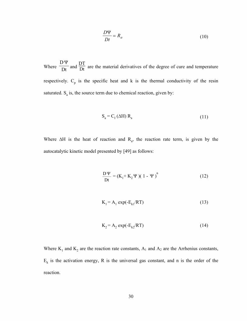
aRDt

D=

Ψ (10)

Where DtD Ψ

and DTDt are the material derivatives of the degree of cure and temperature

respectively. Cp is the specific heat and k is the thermal conductivity of the resin

saturated. Sa is, the source term due to chemical reaction, given by:

Sa = CI (∆H) Ra (11)

Where ∆H is the heat of reaction and Ra, the reaction rate term, is given by the

autocatalytic kinetic model presented by [49] as follows:

Dt

D Ψ = (K1+ K2 Ψ )( 1 - Ψ )n (12)

K1 = A1 exp(-Ek1/RT) (13)

K2 = A2 exp(-Ek2/RT) (14)

Where K1 and K2 are the reaction rate constants, A1 and A2 are the Arrhenius constants,

Ek is the activation energy, R is the universal gas constant, and n is the order of the

reaction.

31

Lumped properties based on weight average thermo-physical properties were used in the

energy and species equations. The properties were determined as follows [39]:

ffrr

fr

ww ρρρρ

ρ+

= (15)

ffrr

fr

wkwkkk

k+

= (16)

pffprrp cwcwc += (17)

)1( ff

rf

ff

VV

Vw

−+=

ρρ

(18)

fr ww −= 1 (19)

Where ρ , fρ , and rρ are the densities of the composite, the fiber, and the resin,

respectively; k , fk , and rk are the thermal conductivities; pc pfc , and prc are the

specific heats of the composite, the fiber, and the resin, respectively; where fw , and

rw are the weight fractions of the fiber mat and the resin respectively; fV is the fiber

volume fraction.

32

4.3 Cure Dependant Mechanical Properties 4.3.1 Fiber Mat Structure To model the mechanical properties of carbon fiber mat composites, the geometry of the

mat was analyzed at microscopic level. Figure 4-8 shows a schematic of a top view of

eight-harness (8H) weave. This number (8H) refers to the number of yarns that are passed

over by one yarn. In an eight harness satin weave, yarns are weaved by passing over

seven and under one yarn before the pattern repeats itself. The fiber yarns which run in x-

direction are called the fill yarns, and those running in the y-direction are called the warp

yarns, with the same fibers count in both directions.

The cross section of some samples produced by VARIM were prepared, polished, and

analyzed under optical microscope. Figure 4-9-(b) shows the shape of a cross section

through the thickness of the molded sample. All the dimensions of the fill and warp yarn

were obtained from the observation under the microscope and this shape was redrawn in

CAD system as shown in Figure 4-9-(a). These observations showed that the warp yarn,

which crosses over the fill yarn, looks like an ellipse. Due to the high compression in

VARIM process, the following seven yarns, which cross under the fill yarn, regroup

together to act as a one bundle.

The analysis is performed on a unit cell which represents the entire mat. The geometry of

eight-harness mat repeats itself every eight yarns in both x- and y-directions. The unit cell

chosen for the analysis should contain all the patterns present in the mat. The complete

unit cell for eight-harness mat consists of eight rows. Figure 4-10 shows the geometry of

33

eight-harness carbon fiber mat as was seen under the microscope. Each section represents

a cross section of the mat along the y-direction, as shown in Figure 4-8. These sections

were used in modeling the composite mechanical properties and sitting up the stiffness

matrices.

Figure 4-8. Schematic of a top view of eight-harness carbon fiber mat.

34

Figure 4-9. Geometry of a cross section of eight-harness carbon fiber mat, (a) a CAD

drawing (b) a picture obtained by optical microscope for sample produced by VARIM.

Figure 4-10. Geometry of eight-harness carbon fiber mat. Each section represents a cross section of the mat along the y-direction.

(a)

(b)

35

4.3.2 Shape Function Formulation The shape function was formulated based on the observation of the cross section of

molded samples by VARIM under the microscope. The fill yarn was modeled as a sin

wave, Figure 4-11 shows the CAD drawing for one layer of the fiber mat, with the fill

yarn as a sin wave. The figure shows also a picture obtained by optical microscope for a

sample produced by VARIM.

Figure 4-11. Geometry of a cross section of eight-harness carbon fiber mat, (a) a CAD drawing (b) a picture obtained by optical microscope for sample produced by VARIM.

Figure 4-12. Geometrical relation between the fill yarn and the warp yarn of 8H fiber

mat.

36

The geometrical relation between the fill yarn and the warp yarn of eight-harness fiber

mat, as shown in Figure 4-12, was used to define the shape function based on the shape

characterization performed by Ito and Chou [50].

The center line of the fill yarn oz is defined as:

)2sin(2

)( xa

hxz zo

π−= where

≤≤−

43

4axa (20)

The fill yarn thickness, zh , is assumed to be constant. The upper boundary of the fill yarn is defined as:

2)()( z

ouhxzxz += (21)

And the lower boundary of the fill yarn is defined as:

2)()( z

olhxzxz −= (22)

The shape of the warp yarn cross section, based on the observation under the microscope,

is assumed to be elliptical and given as:

czggg

t hhxxaxxxa

hxz −+−−−−

= )22)(22(4

2)( 2

where

−≤≤ )

2( gg xaxx (23)

Based on the geometrical shape the variable, ch in the previous equation is defined as:

)12

(sin(2

+=axhh gz

c

π (24)

The local angle between fiber direction and x-axis is:

))((tan)( 1

dxxdzx o−=θ (25)

37

Where, in the previous equations:

oz : center line of fill yarn

uz : upper boundary of the fill yarn

lz : lower boundary of the fill yarn

zh : yarn thickness

a : wavelength of a yarn

tz : boundary of elliptical shape of warp yarn

gx : offset distance of the warp yarn from zero coordinate

θ : angle between fiber direction and x-axis

Some samples of the molded composite material, produced by VARIM, were polished

and observed using an optical microscope. Measurements were made, under the

microscope, for wavelength of a yarn, yarn thickness, elliptical shape of the warp yarn,

and some other necessary dimensions to draw the cross section in CAD system. The area

of the elliptical shape of the warp yarn, and the total fiber bundle cross section area were

used to calculate the bundle fiber volume fraction.

38

4.3.3 Stiffness Matrix Formulation

Classical Laminate Theory (CLT) is assumed to be applicable to the infinitesimal regions of the composite unit cell. The in-plain stiffness constants for each infinitesimal length (dx) are given as follows:

∫=H

0ij

2ijijij dz)Qzz,(1,y)(x,Dy),(x,By),(x,A (26)

=

xy

ν

y

ν

xyx

ν

xyx

ν

x

ij

G00

0DE

DEν

0DEν

DE

Q (27)

Where:

Aij: extensional stiffnesses

Bij: bending-extension coupling stiffnesses

Dij: bending stiffnesses

Qij: reduced stiffnesses

Dν = 1 − νxyνyx

The stiffnesses of the fill, warp, and the matrix are evaluated based on the properties of

each constituent. The fiber volume fraction of the fill and warp was calculated based on

the dimension obtained under the microscope for the shape of the yarn and the total cross

section area of the fiber in the bundle. The bundle fiber volume fraction was found to be

39

62%. The properties of the fill and warp yarn are determined based on the rule of

mixtures as follows:

The longitudinal Young’s modulus of the yarn is given by:

E1 = VfEf + (1-Vf)Em (28)

The transverse Young’s modulus of the yarn, using Halphin and Tsi semi-empirical

models [51], is given by:

)1

1(2

f

fm V

VEE

ηξη

−

+= (29)

))/(

1)/(ξ

η+

−=

mf

mf

EEEE

(30)

The reinforcing factor “ξ ” is given by the empirical formula [52]:

10401 fV+=ξ (31)

The shear modulus is given by:

)1

1(12

f

fm V

VGG

ηξη

−+

= (32)

40

))/(

1)/(ξ

η+

−=

mf

mf

GGGG

(33)

G23 = Gm/(1 - Vf1/2

(1 - Gm/G23f)) (34)

The Poisson’s ratios is given by:

mfff VV ννυυ )1(1312 −+== (35)

1121221 / EEνυ = (36)

)2( 212323 ννυυ −+= mmff VV (37)

Where Em and Ef are the tensile moduli for the matrix and the fiber respectively. Vf is the

fiber volume fraction. Gm and Gf are the shear moduli for the matrix and the fiber

respectively. mν is the Poisson’s ratio for the matrix and fν for the fiber.

The changes in fiber orientation due to yarn undulation must be taken into account. The

effective elastic constants for the fill and warp yarns are given as follows:

θθνθθ 22

1

12

121

4

1

4

cossin21sincos1

−++=

EGEEEx (38)

2EE y = (39)

41

−+−+= θθθθνν 22

1221

44

1

12 cossin111)cos(sinGEEE

Exxy (40)

)cos(sin1cossin142221 44

12

22

121

12

21

θθθθν++

−++=

GGEEEGxy (41)

While the molded composite material using the eight-harness fiber mat is considered to

be orthotropic, the matrix (resin) is considered to be isotropic. At the early stages of

curing, before gelation, resin acts as a liquid. As the degree of cure increases, more cross

linking occurs, and the resin acts as a solid media. The mechanical properties of resin

change as a function of degree of cure. Figure 4-13 shows a linear relation between the

degree of cure and the mechanical properties of the resin. This model was presented in

early ninety and used after that successfully in different studies [39]. This model was

used to determine resin mechanical properties as a function of degree of cure. These

properties are then used to determine the stiffness matrix for the matrix (resin).

Degree of Cure (%)0 5 85 100

E0.5

ν xy

Elastic Modulus

Poisson's Ratio

Figure 4-13. Variation of resin elastic modulus and Poisson’s ratio with cure [39].

42

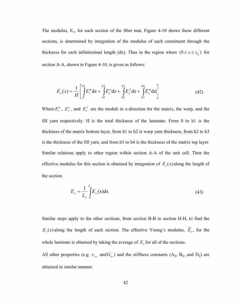
The modulus, Ex, for each section of the fiber mat, Figure 4-10 shows these different

sections, is determined by integration of the modulus of each constituent through the

thickness for each infinitesimal length (dx). Thus in the region where )0( gxx ≤≤ for

section A-A, shown in Figure 4-10, is given as follows:

+++= ∫∫∫∫

4

3

3

2

2

1

1

0

dzdzdzdz1)(h

h

mx

h

h

fx

h

h

wx

hmxx EEEE

HxE (42)

Where mxE , w

xE , and fxE are the moduli in x-direction for the matrix, the warp, and the

fill yarn respectively. H is the total thickness of the laminate. From 0 to h1 is the

thickness of the matrix bottom layer, from h1 to h2 is warp yarn thickness, from h2 to h3

is the thickness of the fill yarn, and from h3 to h4 is the thickness of the matrix top layer.

Similar relations apply to other region within section A-A of the unit cell. Then the

effective modulus for this section is obtained by integration of )(xEx along the length of

the section.

∫=xL

xx

x EL

E0

(x)dx1 (43)

Similar steps apply to the other sections, from section B-B to section H-H, to find the

)(xEx along the length of each section. The effective Young’s modulus, xE , for the

whole laminate is obtained by taking the average of xE for all of the sections.

All other properties (e.g. xyν and xyG ) and the stiffness constants (Aij, Bij, and Dij) are

obtained in similar manner.

43

4.4 Discussion of Cure Modeling Results

4.4.1 Thermal and Cure Analysis Results

The three dimensional transient energy and kinetic equations are nonlinear and coupled

through the source term. These equations were solved using a control volume based

finite difference technique [53]. The exothermic chemical reaction in the 5250-4 RTM

resin releases heat and acts as a heat source. Therefore the energy and the spices

equations, equations 8 and 9, were solved together simultaneously. A MATLAB code

was written, using a control volume based finite difference, to solve for the thermal and

cure histories in the cure cycle. Temperature field is determined in the part at each time

step. Then, the degree of cure is determined by integration of equation 10 with time.

The reaction kinetics, for 5250-4-RTM resin, was determined by using a differential

scanning calorimeter (DSC) [49]. The DSC measured the reaction exthotherm as a

function of time as shown in equations from 12 to 14. Table 4-1summarizes the

parameters of the kinetic model, obtained from reference [49]. Heat of reaction, ∆H in

Table 4-1, was obtained from, the resin manufacturer, CYTEC Engineered Materials

Company [14].

Table 4-1. Kinetic parameters for 5250-4-RTM resin

Arrhenius constant, A1 (1/s)

Arrhenius constant, A2 (1/s)

Activation Energy,

Ek1 (kJ/mole)

Activation Energy,

Ek2 (kJ/mole)

Heat of Reaction, ∆H (kJ/kg)

Order of Reaction,

n

0.815 40.2 29.3 37.3 249.8 2

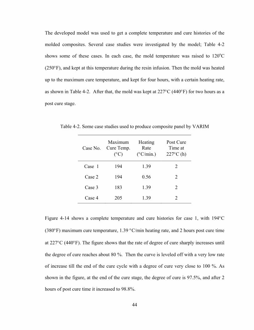
44

The developed model was used to get a complete temperature and cure histories of the

molded composites. Several case studies were investigated by the model; Table 4-2

shows some of these cases. In each case, the mold temperature was raised to 120oC

(250°F), and kept at this temperature during the resin infusion. Then the mold was heated

up to the maximum cure temperature, and kept for four hours, with a certain heating rate,

as shown in Table 4-2. After that, the mold was kept at 227°C (440°F) for two hours as a

post cure stage.

Table 4-2. Some case studies used to produce composite panel by VARIM

Case No. Maximum

Cure Temp. (°C)

Heating Rate

(°C/min.)

Post Cure Time at

227°C (h)

Case 1 194 1.39 2

Case 2 194 0.56 2

Case 3 183 1.39 2

Case 4 205 1.39 2

Figure 4-14 shows a complete temperature and cure histories for case 1, with 194°C

(380°F) maximum cure temperature, 1.39 °C/min heating rate, and 2 hours post cure time

at 227°C (440°F). The figure shows that the rate of degree of cure sharply increases until

the degree of cure reaches about 80 %. Then the curve is leveled off with a very low rate

of increase till the end of the cure cycle with a degree of cure very close to 100 %. As

shown in the figure, at the end of the cure stage, the degree of cure is 97.5%, and after 2

hours of post cure time it increased to 98.8%.

45

Figure 4-15 shows the distribution of degree of cure through the thickness and along the

length of the composite panel for case 1 during curing stage, after one hour from the

beginning of the cure cycle. Figure 4-16 shows the same distribution through the

thickness and along the width of the panel. These two sections were taken at the middle

of the panel. A section at the middle is a good representative for the panel, based on the

observation of several sections taken along the length and the width with almost no

difference. The two figures show that the distribution of degree of cure for any layer

along the length or the width is almost constant except at the edges. But the main change

occurs across the panel thickness, where the degree of cure decreases gradually from the

bottom to the top within a range of 1.8%, from 81.3 to 79.5%. Figure 4-17 shows the

temperature distribution through the thickness and along the length of the composite

panel for case 1 at the of the cure cycle. The temperature distribution shows a trend

similar to the distribution of degree of cure. At the end of the cure cycle, the degree of

cure is almost the same across the part as shown in Figure 4-18.

Another case was studied, case 2, with a low heating rate 0.56°C/min, but with the same

cure temperature and post cure time as in case 1. The complete temperature and cure

histories for case 1 are shown in Figure 4-19. Figure 4-20 shows a comparison for the

cure histories for these two cases, 3 and 4. In case 1, with a higher heating rate, it took the

material 66 minutes to reach about 80% degree of cure, while in case 2, with a lower

heating rate, it took about 115 minutes to reach the same degree.

46

The effect of maximum cure temperature on the trend of degree of cure was studied

through the comparison of two cases, 3 and 4, with the same heating rate and post cure

time but with different maximum cure temperature. In case 3 the maximum cure

temperature was 183oC (360°F), while it was 205oC (400°F) in case 4. Figure 4-21 shows

a comparison for the cure histories for these two cases. In the first hour of the cure cycle,

the degree of cure for both cases was the same. Then the case with the higher cure

temperature reached a higher degree of cure than the case with the lower one. Both cases

reached the same degree of cure at the end of the cure stage and right before the post cure

stage.

0

0.1

0.2

0.3

0.4

0.5

0.6

0.7

0.8

0.9

1

0.0 1.0 2.0 3.0 4.0 5.0 6.0 7.0 8.0

Time, h

Deg

ree

of C

ure,

%

100

125

150

175

200

225

250

Tem

pera

ture

, deg

. C

Degree of CureTemperature

Figure 4-14. Cure and temperature histories for case 1.

47

Figure 4-15. Distribution of degree of cure through the panel thickness along the length.

Figure 4-16. Distribution of degree of cure through the panel thickness along the width.

0.735

0.757

0.745

0.735

0.757

0.745

48

Figure 4-17. Distribution of temperature through the panel thickness along the length.

Figure 4-18. Distribution of degree of cure through the panel thickness along the length.

192.6

193.3

192.9

0.98804

0.98816

0.98810

oC

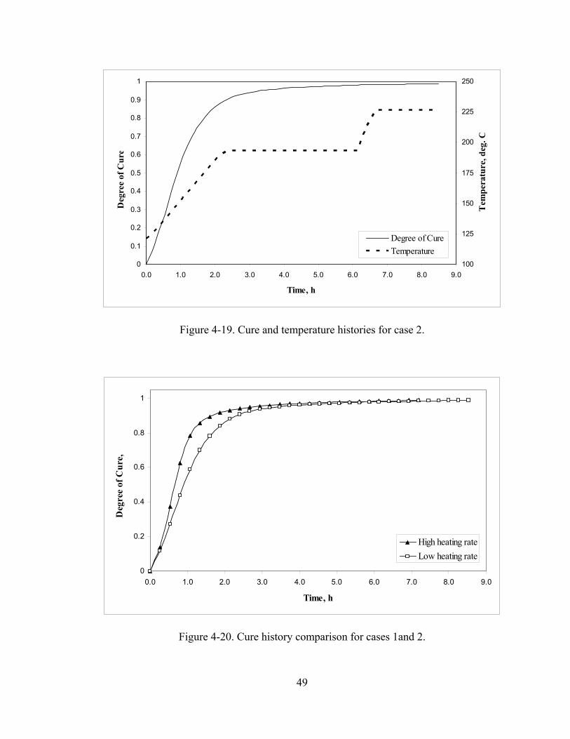
49

0

0.1

0.2

0.3

0.4

0.5

0.6

0.7

0.8

0.9

1

0.0 1.0 2.0 3.0 4.0 5.0 6.0 7.0 8.0 9.0

Time, h

Deg

ree

of C

ure,

%

100

125

150

175

200

225

250

Tem

pera

ture

, deg

. C

Degree of CureTemperature

Figure 4-19. Cure and temperature histories for case 2.

0

0.2

0.4

0.6

0.8

1

0.0 1.0 2.0 3.0 4.0 5.0 6.0 7.0 8.0 9.0

Time, h

Deg

ree

of C

ure,

%

High heating rateLow heating rate

Figure 4-20. Cure history comparison for cases 1and 2.

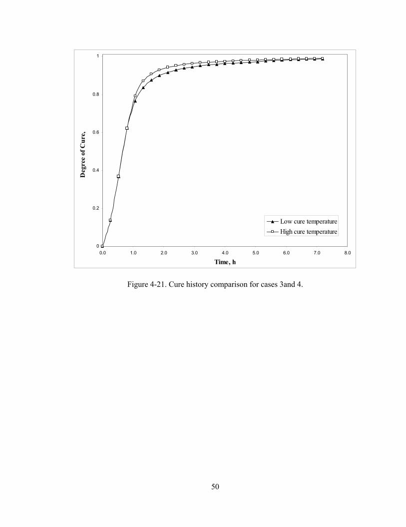
50

0

0.2

0.4

0.6

0.8

1

0.0 1.0 2.0 3.0 4.0 5.0 6.0 7.0 8.0

Time, h

Deg

ree

of C

ure,

%

Low cure temperatureHigh cure temperature

Figure 4-21. Cure history comparison for cases 3and 4.

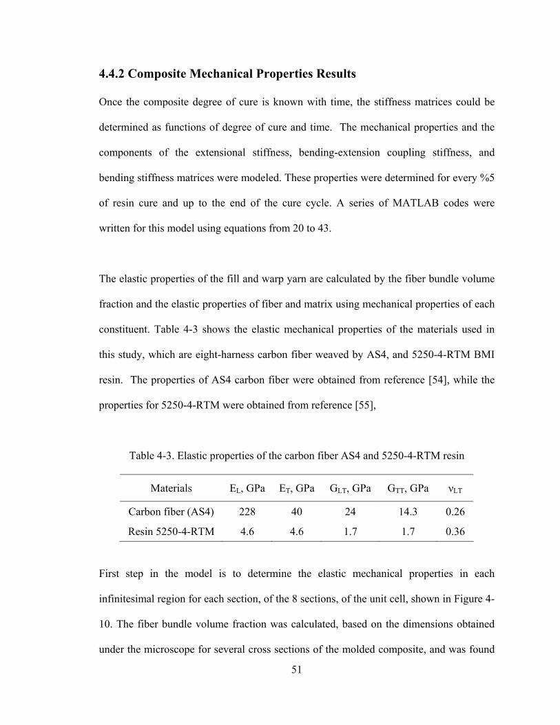
51

4.4.2 Composite Mechanical Properties Results

Once the composite degree of cure is known with time, the stiffness matrices could be

determined as functions of degree of cure and time. The mechanical properties and the

components of the extensional stiffness, bending-extension coupling stiffness, and

bending stiffness matrices were modeled. These properties were determined for every %5

of resin cure and up to the end of the cure cycle. A series of MATLAB codes were

written for this model using equations from 20 to 43.

The elastic properties of the fill and warp yarn are calculated by the fiber bundle volume

fraction and the elastic properties of fiber and matrix using mechanical properties of each

constituent. Table 4-3 shows the elastic mechanical properties of the materials used in

this study, which are eight-harness carbon fiber weaved by AS4, and 5250-4-RTM BMI

resin. The properties of AS4 carbon fiber were obtained from reference [54], while the

properties for 5250-4-RTM were obtained from reference [55],

Table 4-3. Elastic properties of the carbon fiber AS4 and 5250-4-RTM resin

Materials EL, GPa ET, GPa GLT, GPa GTT, GPa νLT

Carbon fiber (AS4) 228 40 24 14.3 0.26

Resin 5250-4-RTM 4.6 4.6 1.7 1.7 0.36

First step in the model is to determine the elastic mechanical properties in each

infinitesimal region for each section, of the 8 sections, of the unit cell, shown in Figure 4-

10. The fiber bundle volume fraction was calculated, based on the dimensions obtained

under the microscope for several cross sections of the molded composite, and was found

52

to be 62%. The cure dependant properties were determined for the resin in the fiber

bundle and resin-rich regions. The composite mechanical properties were determined for

every 5% of resin degree of cure from zero and up to the end of curing cycle, 100 % for

every section of the 8 sections using equation 38 and 39. Figure 4-22 shows the

distribution of Young’s modulus for section A-A at the end of cure cycle. Figure 4-23

shows the change in the modulus due to fiber undulation for the same section. Then, the

average of the modulus through the thickness and along the section length was

determined by equation 42 for each section of the unit cell. A curve represents this

average is shown in Figure 4-24. Figure 4-25 shows the average for every section of the 8

sections, of the unit cell, along x-direction.

Figure 4-22. Distribution of Young’s modulus for section A-A at the end of cure cycle.

GPa

Fill 143 GPa

Fill 143 GPa

Fill 80 GPa

Warp 18 GPa

53

Figure 4-23 Distribution of Young’s modulus at an area with fiber undulation.

Figure 4-24. Average of Young’s modulus through the thickness and along the length.

Matrix 4.6 GPa

Warp 18 GPa

Fill 80 GPa

GPa

Fill 143 GPa

Fill 143 GPa

Fill 80 GPa

Fill 143 GPa

Warp 18 GPa

54

Section H-H40.050.060.070.080.090.0

0

Ex, G

Pa

Section G-G40.050.060.070.080.090.0

0

Ex, G

Pa

Section F-F40.050.060.070.080.090.0

0

Ex, G

Pa

Section E-E40.050.060.070.080.090.0

0

Ex, G

Pa

Section D-D40.050.060.070.080.090.0

0

Ex, G

Pa

Section C-C40.050.060.070.080.090.0

0

Ex, G

Pa

Section B-B40.050.060.070.080.090.0

0

Ex, G

Pa

Section A-A40.050.060.070.080.090.0

0

Section Length

Ex, G

Pa

Figure 4-25. Average of Young’s modulus through the thickness and along the length.

55

The distribution of the effective modulus of the unit cell, as shown in Figure 4-26, was

determined by taking the average for the 8 sections along the y-direction for a one-layer

laminate of carbon fiber mat. A laminate with several layers of carbon fiber randomly

distributed, as shown in Figure 4-27, reduced the wavy distribution of the effective

modulus. Figure 4-28 shows this distribution for a 6-layer laminate.

The previous steps were repeated to determine the modulus of the laminate at every 5 %

of resin degree of cure. The rest of the elastic properties were determined in similar

manner. Figure 4-29 shows the variation of Young’s modulus with resin degree of cure.

The modulus showed an exponential increase with resin degree of cure.

The value of Young’s modulus obtained experimentally in this study, as will be presented

in section 6.3.2, is 15% less than the value obtained by the mathematical model at 100%

degree of cure, shown in Table 4-4. The difference is due to two main reasons; first one is

the assumptions of the mathematical model which assumes that there is no interfacial

sliding between fiber/matrix or between the layers of the fiber mats. Also, no void in the

molded composite was assumed, while the experimental investigation showed a 0.25%

average void content. The second reason is due to the difficulties in the experimental

investigation, which includes the difficulty to lay up the carbon fiber mats parallel to each

other on the top of the mold, and also the difficulty in the machining of the tested

specimens with their sides parallel to the direction of the fibers inside the molded panels.

These reasons result in a higher value of the mathematical model and in a lower value of

the experimentally tested specimens.

56

Average from Sec. A-A to Sec. H-H40.050.060.070.080.090.0

0

Section Length

Mod

ulus

Ex,

GPa

Figure 4-26. Average of Young’s modulus through the thickness and along the length for

the 8 sections of the unit cell of a one-layer laminate.

Figure 4-27. A laminate with six layers of carbon fiber randomly distributed.

Average from Sec. A-A to Sec. H-H for 6 layers40.050.060.070.080.090.0

0

Section Length

Mod

ulus

Ex,

GPa

Figure 4-28. Average of Young’s modulus through the thickness and along the length for

the 8 sections of the unit cell of a six-layer laminate.

57

40.0

45.0

50.0

55.0

60.0

65.0

70.0

75.0

80.0

0.00 20.00 40.00 60.00 80.00 100.00

Degree of Cure, %

You

ng's

Mod

ulus

Ex,

GP

a

Figure 4-29. Variation of Young’s modulus with resin degree of cure.

Tabale 4-4. Cure dependent properties for carbon fiber/5250-4-RTM resin

Degree of Cure, % Ex, GPa Ey, GPa Gxy, GPa νxy

20 61.5 61.5 1.4 0.215

40 66.9 66.9 2.7 0.207

60 70.7 70.7 3.8 0.201

80 73.9 73.9 5.0 0.195

100 74.0 74.0 5.1 0.194

58

Once the effective elastic properties were determined with degree cure, Table 4-4

summarize these properties, the stiffness matrix, Qij, and the stiffness constants Aij, Bij,

and Dij were determined by equations 26 and 27. Figure 4-30, 4-31, and 4-32 show the

variation of the first component of the extensional stiffness, the bending-extension

stiffness, and the bending stiffness, respectively. The extensional stiffness A11 showed an

exponential increase with the resin degree of cure. The bending-extension stiffness and

the bending stiffness showed a similar trend. The non-zero element of the bending-

extension stiffness matrix implies that the normal and shear forces will result in twisting

and bending of the composite part.

1.90E+07

2.10E+07

2.30E+07

2.50E+07

2.70E+07

2.90E+07

3.10E+07

0.00 20.00 40.00 60.00 80.00 100.00

Degree of Cure, %

Exte

nsio

nal S

tiffn

ess

A 11,

N/m

Figure 4-30. Variation of extensional stiffness with resin degree of cure.

59

3.00E+03

4.00E+03

5.00E+03

6.00E+03

7.00E+03

8.00E+03

0.00 20.00 40.00 60.00 80.00 100.00

Degree of Cure, %

Bend

ing-

Exte

nsio

n S

tiffn

ess

B11

, Pa

m2

Figure 4-31. Variation of bending-extension stiffness with resin degree of cure.

0.50

0.70

0.90

1.10

1.30

1.50

1.70

1.90

2.10

2.30

0.00 20.00 40.00 60.00 80.00 100.00

Degree of Cure, %

Bend

ing

Stiff

ness

D11

, Pa

m3

Figure 4-32. Variation of bending stiffness with resin degree of cure.

60

CHAPTER 5

EXPERIMENTAL INVESTIGATION OF VARIM PROCESS

5.1 Introduction

In Vacuum Assisted Resin Infusion Molding (VARIM) process, composite panels of 380

mm (15in) length and 175 mm (7in) width with two different thicknesses, 2.1mm

(0.084in) and 0.79 mm (0.031in), are molded. Vacuum Assisted Resin Infusion Molding

(VARIM) process using single vacuum port and single resin inlet port system is used to

evaluate the feasibility of the process to produce a composite structure with properties

needed for aerospace application. The volume fraction of the fiber in the composite is

maintained at about 58%.

5.2 Materials

Eight harness carbons woven satin fabrics, made of AS4 carbon fiber, are used in the

present composite system to provide the needed reinforcing component and to satisfy the

condition of porous media, required by VARIM process.

The high temperature resin used is CYCOM 5250-4-RTM produced by CYTEC

Engineered Materials in California. It is a one-part homogenous Bismaleimide (BMI)

resin with some additives to improve toughness. This polymer was developed for use in

61

high performance structural composites requiring high temperature up to 204 ºC (400 °F)

use and increased toughness.

5250-4 RTM is a 3-componant modified bisbaleimide (BMI) resin. BMI resins are used

for high performance applications due to their high temperature resistance, high glass

transition temperature, and excellent chemical corrosion resistance. But the main

disadvantage of BMI resins that they are very brittle. 5250-4 RTM resin has three

different components to overcome the disadvantage of MBI resin and to improve

processing and toughness. These three components are Bismalieimidodiphenylmethane

(BMPM) (44 wt%), Diallyl Bisphenol A (DABPA) (32 wt%), and BMI-1, 3-tolyl (24

wt%) [61]. Figure 5-1 illustrates the chemical structures of the three components. The

chemical structure of the combined 3-component 5250-4 RTM resin is shown in Figure

5-2.

It’s known that resins based on BMIs need to be cured at high temperature and postcured

at elevated temperature for relatively longer time. The cross linking mechanism during

cure and postcure process involves two main steps. First step is the opening of carbon-

carbon double bonds (C=C). This step improves the thermal and mechanical properties of

the composite. In the second step with more heating time, the cross linking may occur via

dehydration of the hydroxyl groups. This step leads to microcraking and hence the

deterioration of mechanical properties of composites. This means that longer postcure

time may not improve the mechanical properties [62].

62

Figure 5-1. Chemical structures of 5250-4 RTM resin components, taken from.

Figure 5-2. Chemical structure of the combined 3-component 5250-4 RTM resin.

Hydroxyl group

C = C bond

63

5.3 Experimental Procedure

The experimental procedure for the vacuum assisted resin infusion molding process can

be summarized as follows:

1- The surface of a flat Aluminum mold, with a 560mm (22in) length, 255mm (10in)

width, and 50mm (2in) thick, is cleaned and sprayed with a release agent dry

lubricant (Miller-Stephenson #MS-122AD).

2- A release film, with 510mm (20in) length and 200mm (8in) width, which

enhances the resin flow, is laid on the top of the mold. The release film is a

product of Airtech Int’l, Inc. #A4000.

3- A peel ply material (fiberglass coated with a release agent), with 485mm (19in)

length and 190mm (7.5in) width, is placed on the top of the release film to

prevent the sticking of the preform with the mold. The peel ply material is a high

permeable material to allow resin flow to pass through it. The peel ply is a

product of Airtech Int’l, Inc. bleeder lease.

4- The carbon fiber mat is cut to the required size, which is 380mm (15in) length and

175mm (7in) width, and then stacked one by one on the top of the peel ply. The

carbon fiber mat is produced by Hexcel Schwebel #AGP370-8HBA-49.

5- Another peel ply sheet is laid on the top layer of the carbon fiber (preform). This

sheet prevents the sticking of the preform with the rest of the bagging materials on

the top; also it allows resin flow from the top to the preform.

6- Highly porous materials of fiberglass cloth and Aluminum screen are laid on the

top of the peel ply to accelerate resin flow. The Aluminum screen is 485mm

64

(19in) length and 190mm (7.5in) width with 0.56mm (0.022in) thick. The size of

the screen net is 18-cell in 25mm (1in).

7- A high temperature sealant tape, which seals off the vacuum bag, is applied on the

edge of the mold all around the sides. The tape is a product of Airtech Int’l, Inc.

GS#213-3.

8- A high temperature vacuum bag, with 510mm (20in) length and 330mm (13in)

width, is used to cover the whole top of the mold including the sealant tape. The

vacuum bag is produced by Airtech Int’l, Inc. #WN1500.

9- Two vacuum valves are connected to both sides of the mold, one of them is a

resin inlet and the other is a resin outlet or a vacuum port. The base of the valve is

placed under the vacuum bag and the rest of the valve is attached to the valve base

through the vacuum bag. The vacuum valve is a product of Airtech Int’l, Inc.

VAC valve 399.

10- Vacuum pressure 735mm (29in) of mercury is applied under the bagging to

withdraw the air within the mold.

11- The resin, which is in a solid state at room temperature, is melted in a vacuum

oven at 120oC (250oF) to get all the gases out of it.

12- The tool is then heated to 120oC (250oF) using a heat blanket, with 610mm (24in)

length, and 305mm (12in) width, to have an isothermal resin injection. The heat

blanket, with 120V, 12A, and 1kW, is a product of Briskheat #SRL512012X24.

13- The resin is then transferred to an air-circulating oven at 120oC (250oF) and the

mold inlet tube is to be dipped to the bottom of the resin can inside the oven.

14- The inlet valve is then opened and the resin is allowed to infuse within the fabric.

65

15- After the whole preform is infused by the resin the vacuum is reduced to 177mm

(7in) of mercury and the resin supply is closed off.

16- The mold is covered by glass wools as an insulation, and then is heated to the

maximum cure temperature with a certain heating rate and allowed to cure for 4

hours, and then cooled to room temperature immediately or after several hours of

post cure time according to the experimental design.

17- Temperature changes during curing are monitored using an imbedded

thermocouple inside the mold.

Figure 5-3 shows a schematic diagram of the setup. Figures 5-4, 5-5, and 5-6 show some

pictures of the experimental setup of VARIM process.

Figure 5-3. Schematic diagram of the experimental setup.

66

Figure 5-4. VARIM experimental setup-carbon fiber at the top of the mold.

Figure 5-5. VARIM experimental setup-vacuum bag covers the mold.

Figure 5-6. VARIM experimental setup.

67

5.4 Experimental Design

A partial factorial design of experiments was conducted on VARIM for high temperature

resin composites. The process variables in the design includes: maximum curing

temperature, heating rate during the cure stage, and post cure time at higher temperature

after curing. Samples from the produced composites were evaluated for mechanical

properties and damage assessment in the laboratory in order to establish relationships

between process parameters and the properties of VARIM composites.

In order to obtain generality and precision for the developed experimental database for

the process, the experiments needed to generate the required data must be conducted in a

systematic and organized way. The unifying feature of statistically designed experiments

is that all factors of interest are varied simultaneously. In this way, the maximum amount

of information can be extracted with a minimum number of experiments. The response

surface methodology (RMS) [46] is useful for cases where the responses of interest are

influenced by several process factors and where the main objective is to optimize all

these responses. In this method, a low order polynomial is fitted between the response

parameters of the process. A three parameter RSM with central composite design was

adopted. The design involves a fraction of first-order (2n) factorial design, two “star

points” on the axis of each design variable, and one center point. The parameters were

explored at five levels that cover the wide range of process conditions. The levels are

represented by the commonly used codes (-1, +1, 0) on the factorial portion of the design,

and values (-2, +2) on the axial portion. Table 5-1 displays the parameters, their

corresponding levels and values.

68

A total of different 15 experiments, as shown in Table 5-2, were conducted. Each

experiment will be repeated there times in order to have good estimation of experimental

errors.

Table 5-1. Control factor levels corresponding to their coded levels Level Maximum Cure

Temp. (°C) Heating Rate

(°C/min.) Post Cure Time

at 227°C (h) -2 -1 0 1 2

183 188 194 199 205

0.56 0.83 1.11 1.39 1.67

0 2 4 5 6

Table 5-2. Three parameter central composite design

Exp No.

Maximum Cure

Temp. (°C)

Heating Rate

(°C/min.)

Post Cure

Time at 227°C

(h) 1 188 1.67 0 2 188 1.67 4 3 188 1.12 0 4 188 1.12 4 5 199 1.67 0 6 199 1.67 4 7 199 1.12 0 8 199 1.12 4 9 183 1.39 2 10 205 1.39 2 11 194 0.56 2 12 194 0.84 2 13 194 1.39 6 14 194 1.39 5 15 194 1.39 2

69

5.5 Specimens Preparation

The composite parts were cut first using a solid carbide slitting saw on a milling machine.

All precautions were taken to cut the molded panels parallel to fiber direction. A special

fixture was designed to be used for that purpose. Figure 5-7 shows the machining and the

fixture used. Figure 5-8 shows a panel after being cut. Then a band saw was used to cut

all the samples roughly at both edges. Finally the edges of samples were machined on a

milling machine using a carbide end mill with diamond coating to achieve the required

tolerances according the standards. Figure 5-9 shows the machining process. The same

procedure was followed in the preparation of the specimen for tensile test and for

compression test as well.

Figure 5-7. Machining of composite specimen using a special fixture.

Solid Carbide Slitting Saw

70

Figure 5-8. Lateral lines being cut in the composite panel.

Figure 5-9. Machining of the edges of carbon fiber composite specimen.

Diamond Coated End Mill

Composite Specimen

Vacuum

71

5.6 Conditioning Chamber

An environmentally controlled conditioning chamber has been designed and built to

expose the composite specimens molded by VARIM to an atmosphere with a high

humidity as the actual aerospace working condition. The conditioning chamber is shown

in Figure 5-10. The chamber consists of a stainless steel base, and a glass gar. The

chamber is equipped with an electrical heater, a thermocouple, and a vacuum inlet tube.

The setup of the chamber is shown in Figure 5-11. The chamber is connected to a

vacuum pump, a distillated water tank. A pressure gage and a drierite are installed

between the vacuum pump and the inlet valve. The electrical heater and the thermocouple

are connected to a temperature controller.

The specimens were first dried twice in an oven at 160oC (325oF) for two and half hours

and then left to cool down to room temperature. The conditioning chamber was loaded by

the specimens as shown in Figure 5-12. The specimens were first exposed to a vacuum

pressure of 735mm (29in) of mercury for 24 hours. This step was done to take all the

gases out of the specimens. The water inlet valve was opened, and the water got into the

chamber, until it covered the electrical heater, about 25mm (1in) of water height. Due to

that the relative humidity inside the chamber was raised to 100%. The vacuum valve was

closed at that time. The specimens were exposed to 100% relative humidity for 3400

hours (140 days) to reach to saturation condition [55-59]. The chamber temperature was

kept at 80oC (176oF) to accelerate the process of moisture absorption [60].

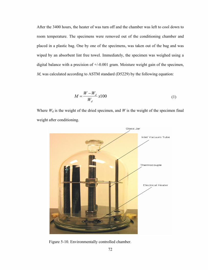
72

After the 3400 hours, the heater of was turn off and the chamber was left to cool down to

room temperature. The specimens were removed out of the conditioning chamber and

placed in a plastic bag. One by one of the specimens, was taken out of the bag and was

wiped by an absorbent lint free towel. Immediately, the specimen was weighed using a

digital balance with a precision of +/-0.001 gram. Moisture weight gain of the specimen,

M, was calculated according to ASTM standard (D5229) by the following equation:

100xW

WWMd

d−= (1)

Where Wd is the weight of the dried specimen, and W is the weight of the specimen final

weight after conditioning.

Figure 5-10. Environmentally controlled chamber.

73

Figure 5-11. Setup of conditioning chamber.

Figure 5-12. Composite specimens loaded in the conditioning chamber.

74

CHAPTER 6

CHARACTERIZATION OF PROPERTIES OF

COMPOSITES MOLDED BY VARIM

6.1 Introduction

In this chapter the feasibility of VARIM for fabricating high temperature polymer matrix

composites was examined. The present study involves the following investigative steps:

1. Physical demonstration of the feasibility of VARIM to produce composite panels

with the desired properties.

2. Evaluation of the effects of the new process on properties and process-induced

damage evolved during VARIM.

3. Development of an empirical relationship between process parameters and the

evolved properties and determination of the optimum process window for the

required properties

4. Comparison of properties of VARIM produced composites with properties

developed using conventional RTM and autoclave/prepreg molding techniques.

75

6.2 Internal Structure of Molded Panels

Several molded panels were inspected for void contents using scanning electron

microscope and image analysis technique. Figure 6-1 displays one of the SEM

micrograph of the internal structure of the molded composites. The average voids

percentage was found to be 0.25%. This is much lower than what normally found in

panels produced by RTM technique (3%). It is also less than what Aerospace industry

would accept in this type of structure (1%). Table 6-1 shows percentage of voids obtained

by image analysis of sectioned samples produced by VARIM. Figure 6-2 shows a sample

report of one of the images analyzed for voids content in the structure.

Figure 6-1. Scanning electron micrograph of composite material produced by VARIM.

76

Figure 6-2. Image analysis micrograph report showing the low micro-voids contents (average 0.25%).

Table 6-1. Percentage of voids obtained by image analysis for some samples produced by VARIM

Micro-void

77

6.3 Characterization of Room-Temperature Tensile Properties

Room temperature tensile strength and tensile modulus of panels produced by VARIM

were determined. Tension test was performed using ASTM standard test method for

tensile properties of polymer matrix composite materials. Designation: D 3039/D

3039M-00. Latest revision: December, 2002.

6.3.1 Test Procedure

The Specimens used in the test are 200 mm (8.0 in) long, 25 mm (1.0 in) wide, and on

average 0.79 mm (0.031 in) thick, to prevent slippage of the specimen inside the

hydraulic grips of the MTS machine; strips of emery cloth were glued to the ends of the

specimen. As shown in Figure 6-3, 64 mm (2.5 in) long by 25 mm (1 in) wide emery

cloth tabs are used on both ends of the specimen. Specimens were placed in the hydraulic

grips of the MTS machine leaving 12.5 mm (0.5 in) of emery cloth showing on top and

bottom. In Figure 6-4, the emery cloth extends past the grips approximately 12.5 mm (0.5

in.) The coupon is shown again in b); the light colored portion of the emery cloth was the

area inside the grips. This practice helps to relieve stress concentrations at the grip edge

by distributing the load on the emery cloth down the sides of the coupon. An

extensometer was used to record strain. The machine which was used in the test is Series

812 Materials Test System from MTS Systems Corporation. Hydraulic grips were used

with a gripping pressure of 10 MPa. The tension test was performed using a constant

head speed of 1.27 mm/min (0.05 in/min).

78

Figure 6-3. Dimensions in millimeter of coupon used in tensile test.

a) b) c)

Figure 6-4. Tension test setup for composite sample, note the emery cloth extends past

the grips approximately 12.5 (0.5 in). The sample is shown again in b); the light colored

portion of the emery cloth was the area inside the grips. A new sample is shown in c).

79

6.3.2 Data Collection

The data was collected and recorded during the test form the extensometer and the MTS

by LABVEIW. The data collected was load in the pounds, ram displacement in inchs,

and strain. The ultimate tensile strength was calculated based on the maximum load

recorded and the dimension measured of the gage length of the sample (width and

thickness). Since the material has a linear response stress-strain curve, the tensile

modulus was calculated as the slope of the linear fit of the stress-strain curve obtained by

LABVEIW. Figure 6-5 shows the stress-strain curve for one of the cases, where the

maximum cure temperature is 188oC (370oF) and the heating rate is 1.67oC/min

(3oF/min) without a post cure time.

0

200

400

600

800

1000

1200

0 0.005 0.01 0.015 0.02

Strain, mm/mm

Stre

ss, M

Pa

Figure 6-5. Stress-strain curve of tensile test for one of the cases.

80

According to ASTM standards the percentage of coefficient of variation of the ultimate

tensile strength and tensile modulus is calculated as follows:

nxxn

ii /)(

1∑

=

= (1)

)1/()( 2

1

21 −−= ∑

=− nxnxS

n

iin (2)

xSCV n /100 1−= (3)

where:

x : sample mean (average)

1−nS : sample standard deviation

CV : sample coefficient of variation, in percent

n : number of specimens

ix : measured property.

Table 6-2 shows the effect of process parameters on ultimate tensile strength. Some cases

were repeated several times to count for error and mistakes. The tensile test for case No.

1 was performed for 21 samples and it came with a coefficient of variation of 7.1 %.

Cases no. 2 and 6 were performed for 10 times and came with a coefficient of variation of

4 and 8.5 % respectively. The average coefficient of variation for the 15 cases was found

81

to be 5.2 %. Table 6-2 also shows the standard deviation and the coefficient of variation

for each case. Figure 6-6 shows the scatter plot for ultimate tensile strength for each case.

The effect of process parameters on the tensile modulus is shown in Table 6-3. The

maximum coefficient of variation was found to be 4.8 % for case No. 1. The average

coefficient of variation for all cases was found to be 3 %. The scatter plot for tensile

modulus for each case is shown in Figure 6-7.

82

Table 6-2. Process parameters effect on ultimate tensile strength for each case

Tensile Strength Case No.

Maximum Cure

Temp. (oC)

Heating Rate

(°C/min.)

Post Cure

Time at 227oC

(h)

No of Samples Tested

Max. Tensile Strength (MPa)

Standard Deviation

Coefficient of

Variation %

1 188 1.67 0 21 917 65 7.1 2 188 1.67 4 10 828 33 4.0 3 188 1.12 0 5 892 69 7.8 4 188 1.12 4 5 804 38 4.7 5 199 1.67 0 8 847 62 7.3 6 199 1.67 4 10 786 66 8.5 7 199 1.12 0 5 841 46 5.5 8 199 1.12 4 5 778 26 3.3 9 183 1.39 2 5 884 24 2.7 10 205 1.39 2 5 817 45 5.5 11 194 0.56 2 5 825 21 2.5 12 194 0.84 2 5 828 35 4.3 13 194 1.39 6 5 838 40 4.7 14 194 1.39 5 5 808 54 6.7 15 194 1.39 2 5 856 34 4.0

Case No.

Max

Str

engt

h, M

Pa

151413121110987654321

1000

800

600

400

200

0

Figure 6-6. Scatter plot of tensile strength for each case shown in table 6-2.

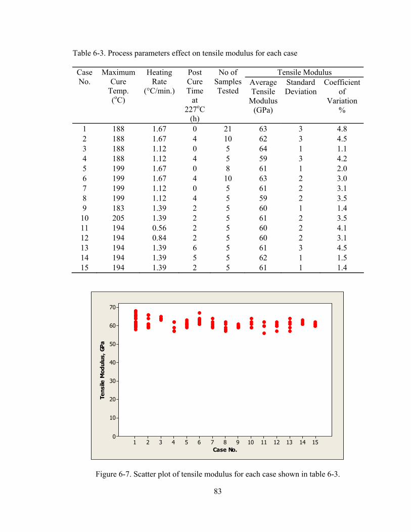
83

Table 6-3. Process parameters effect on tensile modulus for each case

Tensile Modulus Case No.

Maximum Cure

Temp. (oC)

Heating Rate

(°C/min.)

Post Cure Time

at 227oC

(h)

No of Samples Tested

Average Tensile

Modulus (GPa)

Standard Deviation

Coefficient of

Variation %

1 188 1.67 0 21 63 3 4.8 2 188 1.67 4 10 62 3 4.5 3 188 1.12 0 5 64 1 1.1 4 188 1.12 4 5 59 3 4.2 5 199 1.67 0 8 61 1 2.0 6 199 1.67 4 10 63 2 3.0 7 199 1.12 0 5 61 2 3.1 8 199 1.12 4 5 59 2 3.5 9 183 1.39 2 5 60 1 1.4 10 205 1.39 2 5 61 2 3.5 11 194 0.56 2 5 60 2 4.1 12 194 0.84 2 5 60 2 3.1 13 194 1.39 6 5 61 3 4.5 14 194 1.39 5 5 62 1 1.5 15 194 1.39 2 5 61 1 1.4

Case No.

Tens

ile M

odul

us, G

Pa

151413121110987654321

70

60

50

40

30

20

10

0

Figure 6-7. Scatter plot of tensile modulus for each case shown in table 6-3.

84

6.3.3 Response Analysis

The responses obtained from the different 15 cases as shown in Tables 6-2 and 6-3, were

analyzed using graphical representation of the mean effects of each parameter. The

response analysis helps in identifying those parameters that have the greatest impact on

the process. Figures 6-8 to 6-10 show the average main effects of process parameters,

which are post cure time, maximum cure temperature, and heating rate, on ultimate

tensile strength, respectively. These figures show that the trend of the ultimate tensile

strength decreases as the post cure time and the maximum cure temperature increase

within the range used for both parameters. Figure 6-10 shows that as the heating rate

increases form 0.56oC/min (1oF/min) to 1.67oC/min (3oF/min) the composite strength

increases slightly.

Post Cure Time, hour

Mea

n of

Max

Str

engt

h, M

Pa

65420

900

880

860

840

820

800

Figure 6-8. Average main effect of post cure time on ultimate tensile strength.

85

Max Cure Tempraure, °C

Mea

n of

Max

Str

engt

h, M

Pa

205199194188183

900

880

860

840

820

800

Figure 6-9. Average main effect of max cure temperature on ultimate tensile strength.

Heating Rate, °C/min

Mea

n of

Max

Str

engt

h, M

Pa

1.671.391.120.840.56

900

880

860

840

820

800

Figure 6-10. Average main effect of heating rate on ultimate tensile strength.

86

Analysis of variance (ANOVA) was performed to investigate the effect of process

parameters on the obtained responses (maximum tensile strength and tensile modulus).

Table 6-4 summarizes the analysis of variance. The p-values (P) and F-ratios (F) are used

in the analysis to estimate the significance of each parameter on the experimental

responses [63, 64]. F-ratio in the analysis is compared to F a 5%, commonly used, upper

critical value of the F distribution (F table). If F-ratio is greater than F-table, the

parameter is statistically significant. The p-value (P) is compared to level of significance,

α-value. The commonly used value for α is 5%. If p-value is less than or equal to α-

value, the parameter has a significant effect. As shown in Tables 6-4, the p-values for

maximum cure temperature, and post cure time are less than α-value, which is 0.05.

Then, these two parameters within the range used in the experiment are, statistically,

significant factors. F-ratios for maximum cure temperature and post cure time are 5.254

and 10.361 respectively as shown in Table 6-4. The F-ratios confirm the same results as

before, since they are greater than F-table (2.72). Post cure time is the most significant

parameters, as it has the highest F-ratio. The analysis of response, as shown before in

Figures 6-8 and 6-9, shows that these two parameters have strong effect on tensile

strength. The ANOVA shows also that heating rate, with F-ratio less than F-table and p-

value greater than α-value, is an insignificant parameter.

87

Table 6-4. Analysis of variance for ultimate tensile strength

Source Sum Squares DF Mean

Square F P

Max Cure Temp 42124.7 3 14041.6 5.254 0.002 Heating Rate 6217.5 3 2072.5 0.775 0.511 Post Cure Time 83075.8 3 27691.9 10.361 0.000 Error 237872.9 89 2672.73 Total 449794.9 103

Where in the ANOVA tables, the DF is the degree of freedom, F is the error variance

ratio, and P is the percentage of confidence level of the parameters.

Figures 6-11 to 6-13 show the average main effects of process parameters, which are post

cure time, maximum cure temperature, and heating rate, on tensile modulus, respectively.

Figure 6-11 shows that as the heating rate increases the modulus slightly increases. As

shown in Figures 6-12 and 6-13 the effects of post cure time and maximum cure

temperature on tensile modulus are not clear and the data is scattered around the average

line. The analysis of variance (ANOVA), summarized in Table 6-5, shows that post cure

time is the dominant parameter over the other two parameters, heating rate and maximum

cure temperature. The analysis shows that post cure time is slightly significant as its F-

ratio, 2.71, is equal to F-table, 2.72. Heating rate and maximum cure temperature are

insignificant parameters as their F-ratios are less than the F-table.

88

Heating Rate, °C/min

Mea

n of

Ten

sile

Mod

ulus

, GPa

1.671.391.120.840.56

62.5

62.0

61.5

61.0

60.5

60.0

Figure 6-11. Average main effect of heating rate on tensile modulus.

Post Cure Time, hour

Mea

n of

Ten

sile

Mod

ulus

, GPa

65420

62.5

62.0

61.5

61.0

60.5

60.0

Figure 6-12. Average main effect of post cure time on tensile modulus.

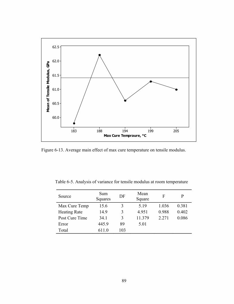
89

Max Cure Tempraure, °C

Mea

n of

Ten

sile

Mod

ulus

, GPa

205199194188183

62.5

62.0

61.5

61.0

60.5

60.0

Figure 6-13. Average main effect of max cure temperature on tensile modulus.

Table 6-5. Analysis of variance for tensile modulus at room temperature

Source Sum Squares DF Mean

Square F P

Max Cure Temp 15.6 3 5.19 1.036 0.381 Heating Rate 14.9 3 4.951 0.988 0.402 Post Cure Time 34.1 3 11.379 2.271 0.086 Error 445.9 89 5.01 Total 611.0 103

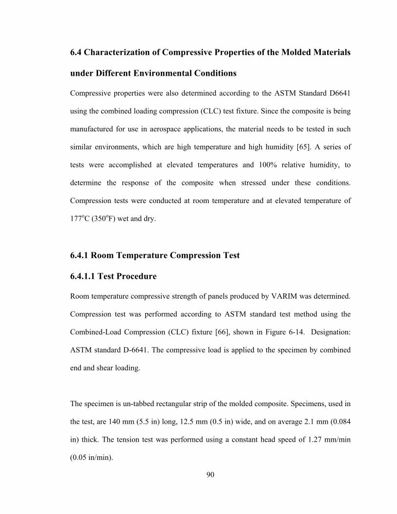
90

6.4 Characterization of Compressive Properties of the Molded Materials

under Different Environmental Conditions

Compressive properties were also determined according to the ASTM Standard D6641

using the combined loading compression (CLC) test fixture. Since the composite is being

manufactured for use in aerospace applications, the material needs to be tested in such

similar environments, which are high temperature and high humidity [65]. A series of

tests were accomplished at elevated temperatures and 100% relative humidity, to

determine the response of the composite when stressed under these conditions.

Compression tests were conducted at room temperature and at elevated temperature of

177oC (350oF) wet and dry.

6.4.1 Room Temperature Compression Test

6.4.1.1 Test Procedure

Room temperature compressive strength of panels produced by VARIM was determined.

Compression test was performed according to ASTM standard test method using the

Combined-Load Compression (CLC) fixture [66], shown in Figure 6-14. Designation:

ASTM standard D-6641. The compressive load is applied to the specimen by combined

end and shear loading.

The specimen is un-tabbed rectangular strip of the molded composite. Specimens, used in

the test, are 140 mm (5.5 in) long, 12.5 mm (0.5 in) wide, and on average 2.1 mm (0.084

in) thick. The tension test was performed using a constant head speed of 1.27 mm/min

(0.05 in/min).

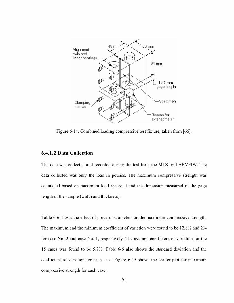
91

Figure 6-14. Combined loading compressive test fixture, taken from [66].

6.4.1.2 Data Collection

The data was collected and recorded during the test from the MTS by LABVEIW. The

data collected was only the load in pounds. The maximum compressive strength was

calculated based on maximum load recorded and the dimension measured of the gage

length of the sample (width and thickness).

Table 6-6 shows the effect of process parameters on the maximum compressive strength.

The maximum and the minimum coefficient of variation were found to be 12.8% and 2%

for case No. 2 and case No. 1, respectively. The average coefficient of variation for the

15 cases was found to be 5.7%. Table 6-6 also shows the standard deviation and the

coefficient of variation for each case. Figure 6-15 shows the scatter plot for maximum

compressive strength for each case.

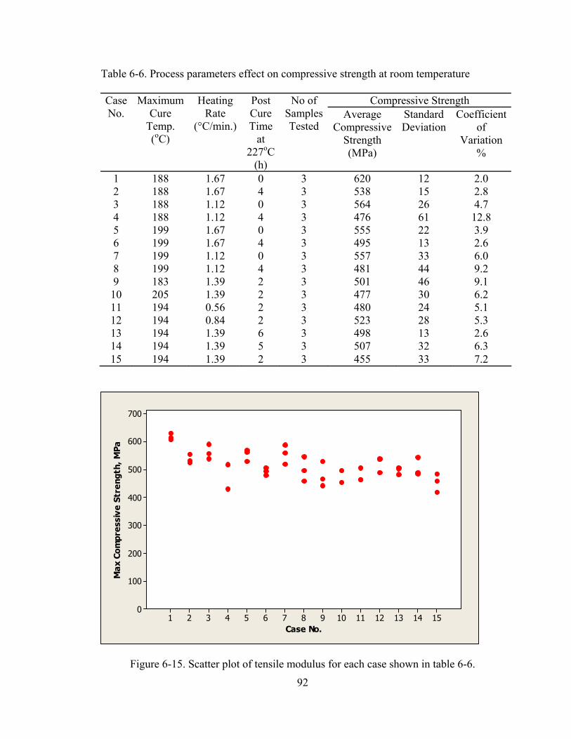
92

Table 6-6. Process parameters effect on compressive strength at room temperature

Compressive Strength Case No.

Maximum Cure

Temp. (oC)

Heating Rate

(°C/min.)

Post Cure Time

at 227oC

(h)

No of Samples Tested

Average Compressive

Strength (MPa)

Standard Deviation

Coefficient of

Variation %

1 188 1.67 0 3 620 12 2.0 2 188 1.67 4 3 538 15 2.8 3 188 1.12 0 3 564 26 4.7 4 188 1.12 4 3 476 61 12.8 5 199 1.67 0 3 555 22 3.9 6 199 1.67 4 3 495 13 2.6 7 199 1.12 0 3 557 33 6.0 8 199 1.12 4 3 481 44 9.2 9 183 1.39 2 3 501 46 9.1 10 205 1.39 2 3 477 30 6.2 11 194 0.56 2 3 480 24 5.1 12 194 0.84 2 3 523 28 5.3 13 194 1.39 6 3 498 13 2.6 14 194 1.39 5 3 507 32 6.3 15 194 1.39 2 3 455 33 7.2

Case No.

Max

Com

pres

sive

Str

engt

h, M

Pa

151413121110987654321

700

600

500

400

300

200

100

0

Figure 6-15. Scatter plot of tensile modulus for each case shown in table 6-6.

93

6.4.1.3 Response Analysis

The responses obtained from the different 15 cases as shown in Table 6-6, were analyzed

using graphical representation of the mean effects of each parameter. Figures 6-16 to 6-

18 show the average main effects of process parameters, which are post cure time,

maximum cure temperature, and heating rate, on max compressive strength. Figure 6-16

shows that the max compressive strength decreases as the post cure time increases within

the range used in the experiments, from zero to 2 hours and then almost stays within the

same range. Figure 6-17 shows that the max compressive strength increases as the

heating rate increases form 0.56oC/min (1oF/min) to 1.67oC/min (3oF/min). Except at

heating rate 1.39oC/min (2.5oF/min) it showed a drop in the compressive strength. The

effect of maximum cure temperature is not clear and the data is scattered around the

average line as shown in Figure 6-18.

Post Cure Time, hour

Mea

n of

Max

Com

pres

sive

Str

engt

h, M

Pa

65420

580

560

540

520

500

480

Figure 6-16. Average main effect of post cure time on compressive strength.

94

Heating Rate, °C/min

Mea

n of

Max

Com

pres

sive

Str

engt

h, M

Pa

1.671.391.120.840.56

580

560

540

520

500

480

Figure 6-17. Average main effect of heating rate on compressive strength.

Max Cure Tempraure, °C

Mea

n of

Max

Com

pres

sive

Str

engt

h, M

Pa

205199194188183

580

560

540

520

500

480

Figure 6-18. Average main effect of max cure temperature on compressive strength.

95

The analysis of variance (ANOVA) shows that post cure time in the range used in the

experiments is the most significant parameter followed by heating rate. As shown in the

ANOVA Table 6-7 p-values for these two parameters are less than the percentage of

confidence, α-value, which is 0.05. F-ratios for these two parameters, heating rate and

post cure time, are 4.166 and 12.196 respectively as shown in Table 6-7. Their F-ratios

confirm the same results as before, since they are greater than F-table (2.83). Also, the

analysis shows that maximum cure temperature is statistically insignificant. The p-value

for maximum cure temperature, 0.243, is greater than the α-value, 0.05.

Table 6-7. Analysis of variance for max compressive strength at room temperature

Source Sum Squares DF Mean

Square F P

Max Cure Temp 4036.8 3 1345.61 1.473 0.243 Heating Rate 11414.6 3 3804.86 4.166 0.015 Post Cure Time 33415.0 3 11138.3 12.196 0.000 Error 25572.0 28 913.286 Total 104222.8 42

96

6.4.2 High Temperature-Dry Compression Test

6.4.2.1 Test Procedure

The effect of elevated temperature on compressive strength and modulus of panels

produced by VARIM were determined. Compression test was performed according to

ASTM standard test method using the Combined-Load Compression (CLC) fixture.

Designation: ASTM standard D-6641. The compressive load is applied to the specimen

by combined end and shear loading. The CLC fixture was modified to be equipped with a

heating coil and a thermocouple. Figure 6-19 shows a picture of the modified fixture. The

thermocouple is connected to a temperature controller to control the heating rate. The

heating coil and the thermocouple are shown in Figure 6-20.

Figure 6-19. Combined load compression (CLC) modified fixture.

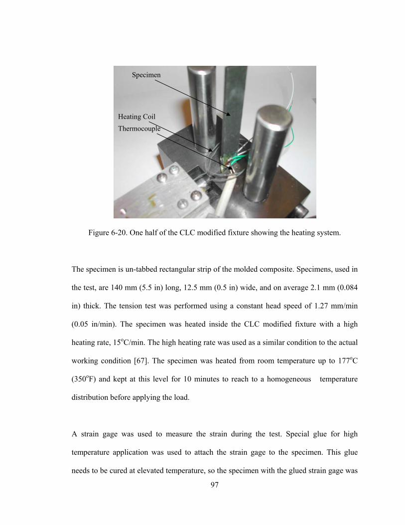
97

Figure 6-20. One half of the CLC modified fixture showing the heating system.

The specimen is un-tabbed rectangular strip of the molded composite. Specimens, used in

the test, are 140 mm (5.5 in) long, 12.5 mm (0.5 in) wide, and on average 2.1 mm (0.084

in) thick. The tension test was performed using a constant head speed of 1.27 mm/min

(0.05 in/min). The specimen was heated inside the CLC modified fixture with a high

heating rate, 15oC/min. The high heating rate was used as a similar condition to the actual

working condition [67]. The specimen was heated from room temperature up to 177oC

(350oF) and kept at this level for 10 minutes to reach to a homogeneous temperature

distribution before applying the load.

A strain gage was used to measure the strain during the test. Special glue for high

temperature application was used to attach the strain gage to the specimen. This glue

needs to be cured at elevated temperature, so the specimen with the glued strain gage was

Thermocouple Heating Coil

Specimen

98

heated at an air circulating oven to 163oC (325oF) for two hours and half with a heating

rate of 15oC/min, as recommended by the manufacturer. Figure 6-21 shows the specimen

used in the test.

Figure 6-21. The specimen with the strain gage used in the compression test.

6.4.2.2 Data Collection

The data was collected and recorded during the test form the MTS by LABVEIW. The

data collected was the compressive load, the corresponding strain, and the specimen

temperature. The maximum compressive strength was calculated based on maximum

load recorded and the dimension measured of the gage length of the sample (width and

thickness). The compressive modulus was calculated as the slope of the linear fit of the

stress-strain curve obtained. Figure 6-22 shows the stress-strain curve for one of the

cases, where the maximum cure temperature is 199oC (390oF) and the heating rate is

1.11oC/min (2oF/min) without post cure time.

Table 6-8 shows the effect of process parameters on the ultimate compressive strength.

The average coefficient of variation for the 15 cases, every case repeated 3 times, was

found to be 7.7 %. Table 6-8 also shows the standard deviation and the coefficient of

variation for each case. Figure 6-23 shows the scatter plot for ultimate compressive

strength for each case.

99

The effect of process parameters on the compressive modulus is shown in Table 6-9. The

maximum coefficient of variation was found to be 11.3 % for case No. 3. Case numbers 2

and 15 have the lowest coefficient of variation, 0.2 %. The average coefficient of

variation for all cases was found to be 3.7 %. The scatter plot for compressive modulus

for each case is shown in Figure 6-24.

0

100

200

300

400

500

600

0 0.002 0.004 0.006 0.008 0.01

Strain, mm/mm

Cpm

pres

sive

Stre

ngth

, MPa

Figure 6-22. Stress-strain curve for compression test of one of the cases.

100

Table 6-8. Process parameters effect on the compressive strength for high temp-dry

Compressive Strength Case No.

Maximum Cure

Temp. (oC)

Heating Rate

(°C/min.)

Post Cure Time

at 227oC

(h)

No. of Samples Tested

Compressive Strength (MPa)

Standard Deviation

Coefficient of

Variation %

1 188 1.67 0 3 533 35 6.5 2 188 1.67 4 3 327 34 10.4 3 188 1.12 0 3 466 47 10.2 4 188 1.12 4 3 358 18 5.0 5 199 1.67 0 3 438 42 9.6 6 199 1.67 4 3 404 33 8.1 7 199 1.12 0 3 391 48 12.2 8 199 1.12 4 3 463 5 1.1 9 183 1.39 2 3 480 46 9.5 10 205 1.39 2 3 396 20 5.0 11 194 0.56 2 3 433 46 10.6 12 194 0.84 2 3 435 45 10.4 13 194 1.39 6 3 444 12 2.7 14 194 1.39 5 3 515 47 9.2 15 194 1.39 2 3 436 23 5.2

Exp. No.

Max

Com

pres

sive

Str

engt

h, M

Pa

151413121110987654321

600

500

400

300

200

100

0

Figure 6-23. Scatter plot of compressive modulus for each case shown in table 6-8.

101

Table 6-9. Process parameters effect on the compressive modulus for each case

Compressive Modulus Case No.

Maximum Cure

Temp. (oC)

Heating Rate

(°C/min.)

Post Cure Time

at 227oC

(h)

No. of Samples Tested

Compressive Modulus

(GPa)

Standard Deviation

Coefficient of

Variation %

1 188 1.67 0 3 61 3 4.7 2 188 1.67 4 3 63 1 1.1 3 188 1.12 0 3 58 7 11.3 4 188 1.12 4 3 63 3 4.1 5 199 1.67 0 3 59 1 1.9 6 199 1.67 4 3 63 3 4.3 7 199 1.12 0 3 65 2 3.1 8 199 1.12 4 3 62 0 0.2 9 183 1.39 2 3 61 1 2.4 10 205 1.39 2 3 64 4 6.7 11 194 0.56 2 3 60 2 4.1 12 194 0.84 2 3 65 0 0.0 13 194 1.39 6 3 62 4 7.0 14 194 1.39 5 3 62 3 4.4 15 194 1.39 2 3 59 0 0.2

Exp. No.

Max

Com

pres

sive

Mod

ulus

, GPa

151413121110987654321

70

60

50

40

30

20

10

0

Figure 6-24. Scatter plot of compressive modulus for each case shown in table 6-9.

102

6.4.2.3 Response Analysis

The responses obtained from the 15 different cases as shown in Tables 6-8 and 6-9, were

analyzed using graphical representation of the mean effects of each parameter. Figures 6-

25 to 6-27 show the average main effects of process parameters, which are post cure

time, maximum cure temperature, and heating rate, on compressive strength,

respectively. Figure 6-25 shows that the compressive strength decreases as the post cure

time increases from zero to 4 hours, and then it increases at post cure time of 5 hours.

After that the strength decreases at post cure time of 6 hours. Figure 6-26 shows that the

trend of compressive strength decreases as the maximum cure temperature increases

except at cure temperature of 194oC (380oF) the strength shows a slight increase. The

heating rate, as shown in Figure 6-27, does not show a clear effect on compressive

strength, since the data is scattered around and close to the average line.

Post Cure Time, hour

Mea

n of

Max

Com

pres

sive

Str

engt

h, M

Pa

65420

520

500

480

460

440

420

400

380

Figure 6-25. Average main effect of post cure time on compressive strength.

103

Max Cure Tempraure, °C

Mea

n of

Max

Com

pres

sive

Str

engt

h, M

Pa

205199194188183

520

500

480

460

440

420

400

380

Figure 6-26. Average main effect of max cure temperature on compressive strength.

Heating Rate, °C/min

Mea

n of

Max

Com

pres

sive

Str

engt

h, M

Pa

1.671.391.120.840.56

520

500

480

460

440

420

400

380

Figure 6-27. Average main effect of heating rate on compressive strength.

104

Analysis of variance (ANOVA) was performed for the obtained responses and

summarized in Table 6-10. The analysis shows that post cure time in the range used in

the experiments is a significant parameter. As shown in Tables 6-10 the p-value for post

cure time, 0.003, is less than the percentage of confidence, α-value, which is 0.05 and its

F-ratio, 6.809, is greater than F-table, 2.90. Also, the analysis shows that the p-value for

heating rate and maximum cure temperature are greater than the α-value. Then, these two

parameters in the range used in the experiment are statistically insignificant.

Table 6-10. Analysis of variance for compressive strength at high temperature-dry

Source Sum Squares DF Mean

Square F P

Max Cure Temp 8730.5 3 2910.18 2.072 0.138 Heating Rate 156.0 3 52.00 0.037 0.990 Post Cure Time 28694.9 3 9564.98 6.809 0.003 Error 26688.7 19 1404.67 Total 118445.8 33

Figures 6-28 to 6-30 show the average main effects of process parameters, which are

maximum cure temperature, post cure time, and heating rate, on compressive modulus,

respectively. Figure 6-28 shows that as the maximum cure temperature increases, in the

range used in the experiment, the modulus slightly increases. As shown in Figures 6-29

and 6-30 the effects of post cure time and heating rate on compressive strength are not

clear and the data is scattered around the average line.

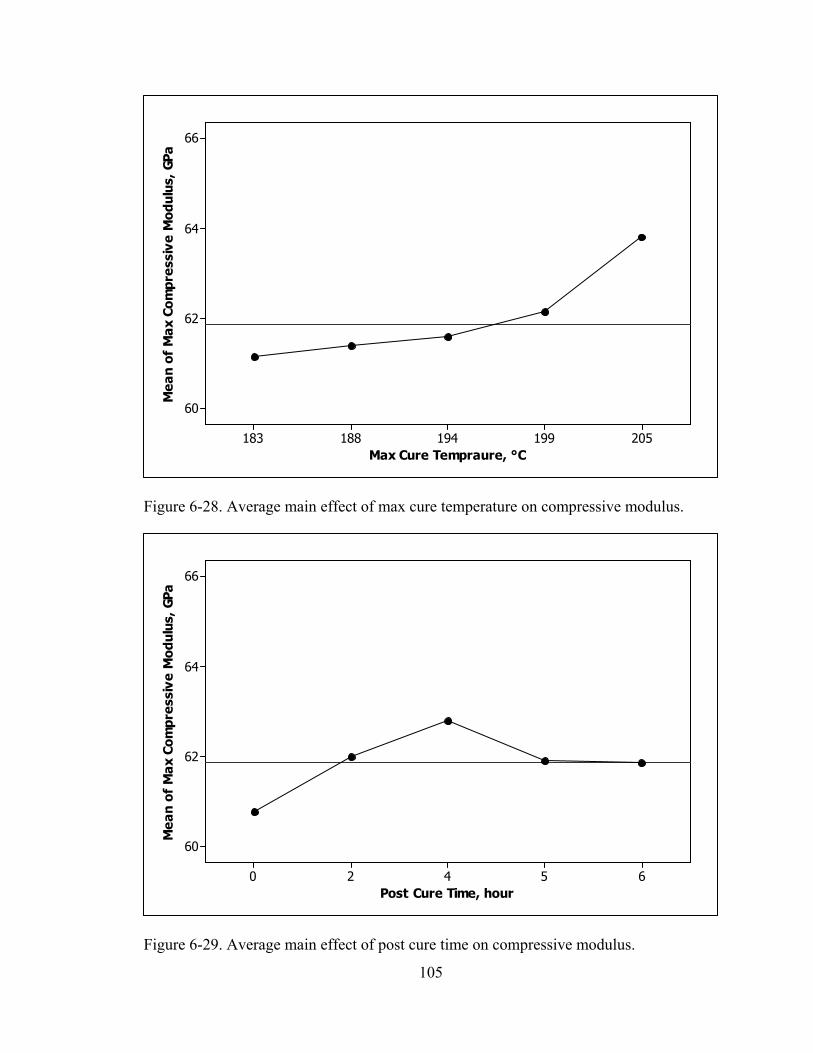
105

Max Cure Tempraure, °C

Mea

n of

Max

Com

pres

sive

Mod

ulus

, GPa

205199194188183

66

64

62

60

Figure 6-28. Average main effect of max cure temperature on compressive modulus.

Post Cure Time, hour

Mea

n of

Max

Com

pres

sive

Mod

ulus

, GPa

65420

66

64

62

60

Figure 6-29. Average main effect of post cure time on compressive modulus.

106

Heating Rate, °C/min

Mea

n of

Max

Com

pres

sive

Mod

ulus

, GPa

1.671.391.120.840.56

66

64

62

60

Figure 6-30. Average main effect of heating rate on compressive modulus.

The analysis of variance shown in Tables 6-11, shows that maximum cure temperature,

heating rate, and post cure time, in the range used in the experiment, are statistically

insignificant for this response (compressive modulus). As shown in the table, the p-values

for these three parameters are less than α-value, which is 0.05. The F-ratios for maximum

cure temperature, heating rate, and post cure time are 1.336, 1.802 and 1.207 respectively

as shown in Table 6-11. The F-ratios confirm the same results as before, since they are all

less than F-table (2.91).

107

Table 6-11. Analysis of variance for compressive modulus at high temperature-dry

Source Sum Squares DF Mean

Square F P

Max Cure Temp 35.2 3 11.721 1.336 0.296 Heating Rate 47.4 3 15.813 1.802 0.185 Post Cure Time 31.8 3 10.592 1.207 0.337 Error 149.1 17 8.773 Total 277.5 31

6.4.3 High Temperature-Wet Compression Test

6.4.3.1 Test Procedure

The same test procedure used in section 6.4.2 for high temperature-dry compression test

was used for high temperature-wet compression test. The same specimen size was also

used. But the main difference is the specimens in this test have been exposed to 100%

relative humidity for 3400 hours (140 days) according to the procedure explained in

section 5.6. The moisture weight gained during this period was found to be 1.05% of the

specimen weight.

The specimen was heated, inside the compression fixture, from room temperature up to

177oC (350oF) and kept at this level for 10 minutes to reach to a homogeneous

temperature distribution before applying the compression load.

A group of 15 specimens, one of each case tested, called “travelers” was conditioned at

100% relative humidity for the same period. These specimens went through the heating

cycle inside the test fixture, but without applying any compression load. Then they were

weighed to determine the actual percentage of moisture gained at the time of the test.

108

Table 6-12 shows the percentage of moisture gain after conditioning and at the time of

test.

Table 6-12. Percentage of weight gain after condoning and at time of test

Specimen No.

Weight gain % after 3400

h at 100% RH

Weight gain % at time of

test

1 1.06 0.88 2 1.07 0.88 3 1.05 0.92 4 1.03 0.85 5 1.04 0.89 6 1.04 0.89 7 1.05 0.87 8 1.07 0.88 9 1.05 0.87 10 1.05 0.87 11 1.06 0.86 12 1.06 0.91 13 1.06 0.87 14 1.04 0.84 15 1.07 0.88

6.4.3.2 Data Collection

The data was collected and recorded during the test form the MTS by LABVEIW. The

data collected is the compressive load and the specimen temperature. The maximum

compressive strength was calculated based on maximum load recorded and the dimension

measured of the gage length of the sample (width and thickness).

109

Table 6-13 shows the effect of process parameters on the ultimate compressive strength.

The average coefficient of variation for the 15 cases, every case repeated 3 times, was

found to be 10.1 %. Table 6-13 also shows the standard deviation and the coefficient of

variation for each case. Figure 6-31 shows the scatter plot for ultimate compressive

strength for each case.

110

Table 6-13. Process parameters effect on the compressive strength for high temp-wet

Compressive Strength Case No.

Maximum Cure

Temp. (°C)

Heating Rate

(°C/min.)

Post Cure Time

at 227°C

(h)

No of Samples Tested

Compressive Strength (MPa)

Standard Deviation

Coefficient of

Variation %

1 188 1.67 0 3 219 28 12.7 2 188 1.67 4 3 286 3 0.9 3 188 1.12 0 3 175 4 2.5 4 188 1.12 4 3 250 33 13.3 5 199 1.67 0 3 307 36 11.7 6 199 1.67 4 3 240 41 17.2 7 199 1.12 0 3 242 15 6.4 8 199 1.12 4 3 300 33 10.9 9 183 1.39 2 3 283 22 7.9 10 205 1.39 2 3 255 24 9.4 11 194 0.56 2 3 259 48 18.6 12 194 0.84 2 3 240 21 8.7 13 194 1.39 6 3 225 13 5.9 14 194 1.39 5 3 301 32 10.6 15 194 1.39 2 3 225 34 15.0

Case No.

Max

Com

pres

sive

Str

engt

h, M

Pa

151413121110987654321

350

300

250

200

150

100

50

0

Figure 6-31. Scatter plot of compressive modulus for each case shown in table 6-13.

111

6.4.3.3 Response Analysis

The responses obtained from the 15 different cases as shown in Table 6-12 was analyzed

using graphical representation of the mean effects of each parameter. Figures 6-32 to 6-

34 show the average main effects of process parameters, which are post cure time,

maximum cure temperature, and heating rate, on compressive strength, respectively.

Figure 6-32 shows that the compressive strength increases as the post cure time increases

from zero to 5 hours, and then it drops sharply at post cure time of 6 hours. Figure 6-31

shows that the maximum compressive strength is at cure temperature of 183oC (360oF).

The heating rate, as shown in Figure 6-34, does not show a clear effect on compressive

strength, since the data is scattered around and close to the average line.

Post Cure Time, hour

Mea

n of

Max

Com

pres

sive

Str

engt

h, M

Pa

65420

320

300

280

260

240

220

Figure 6-32. Average main effect of post cure time on compressive strength.

112

Max Cure Tempraure, °C

Mea

n of

Max

Com

pres

sive

Str

engt

h, M

Pa

205199194188183

320

300

280

260

240

220

Figure 6-33. Average main effect of max cure temperature on compressive strength.

Heating Rate, °C/min

Mea

n of

Max

Com

pres

sive

Str

engt

h, M

Pa

1.671.391.120.840.56

320

300

280

260

240

220

Figure 6-34. Average main effect of heating rate on compressive strength.

113

Table 6-14 summarizes the analysis of variance (ANOVA) conducted for the obtained

responses. The p-values for maximum cure temperature, and post cure time are less than

α-value, which is 0.05. Then, these two parameters within the range used in the

experiment are, statistically, significant parameters. F-ratios for maximum cure

temperature and post cure time are 4.648 and 5.278 respectively as shown in Table 6-14.

The F-ratios confirm the same results as before, since they are greater than F-table (2.88).

Post cure time is the most significant parameters, as it has the highest F-ratio and the

lowest p-value. The analysis of response, as shown before in Figures 6-32 and 6-33,

showed that these two parameters have strong effect on compressive strength. The

ANOVA shows also that heating rate, with F-ratio less than F-table and p-value greater

than α-value, is an insignificant parameter.

Table 6-14. Analysis of variance for compressive strength at high temperature-wet

Source Sum Squares DF Mean Square F P

Max Cure Temp 11851.0 3 3950.34 4.648 0.012 Heating Rate 3704.9 3 1234.97 1.453 0.256 Post Cure Time 13456.2 3 4485.39 5.278 0.007 Error 17846.7 21 849.841 Total 58329.0 35

114

6.5 Discussion of Experimental Results

One of the objectives of this study is to experimentally investigate the effects of the

major process parameters on mechanical properties for composite materials molded by

VARIM. This experimental investigation helps to build a science based technology for

VARIM process to produce composite materials free of defects with the highest possible

mechanical properties suitable for high temperature applications. The major process

parameters, that were investigated, are maximum cure temperature, post cure time, and

heating rate. Mechanical properties were tested under tensile and compressive loads.

Tests were conducted at room temperature and at elevated temperature. A group of

specimens tested were first conditioned at 100% relative humidity to simulate the actual

working condition.

The findings of room temperature tensile and compressive load tests show that post cure

time and maximum cure temperature plays the most significant role in VARIM process.

The response analysis for both tension and compression test confirms that as post cure

time increases, in the range used in the experimental design, the material strength

decreases. The highest strength at room temperature was obtained without a post cure

stage. The effect of maximum cure temperature on room temperature tensile test shows

that as maximum cure temperature decreases in the range used in the experimental

design, tensile strength increases. Also, the highest compressive strength was obtained at

a low cure temperature (188oC). So, both tensile and compressive load test confirms that

a low cure temperature, within the range used in the experimental design, leads to a high

strength.

115

Heating rate, in the range used in the experimental design, does not show a significant

effect on both tensile and compressive strength at room temperature. However, the

response analysis shows that as heating rate increases the strength slightly increases. The

highest heating rate used in this study, which is 1.67oC/min, led to the highest strength.

The findings of room temperature tensile and compressive load tests show that the

compressive strength is about 32% less than the tensile strength. In fact this difference

was explored by Li [55] using composite materials with a different type of carbon fiber.

In his study, there is a 37% reduction in the compressive strength from the tensile

strength. It was found that the most likely damage in the tested specimens is the intra-ply

delamination, which was also observed in this study. It’s obvious that the intra-ply

delamination has a greater effect on compressive strength rather than on tensile strength.

During Cure and post cure stages, the cross linking mechanism involves two main steps,

as explained in section 3.2.1. These two steps are carbon-carbon double bonds (C=C)

opening, and dehydration of hydroxyl groups. First step improves the composite

mechanical properties, while the second step deteriorates the mechanical properties. As

the maximum cure temperature increases the effects of the rate of dehydration becomes

more pronounced as compared with the mechanism of carbon-carbon double bonds

(C=C) opening. Since curing the resin at a high temperature, for the same time as at a low

temperature, increases the possibility of water molecules diffusion out of the polymer,

which leads to more defects. While at a low maximum cure temperature, within the range

used in the experimental design, the carbon-carbon double bonds (C=C) opening

116

dominates the mechanism of cross linking, which improves the composite mechanical

properties.

So, curing time, which is 4 hours in this study, at a low maximum cure temperature,

within the rage used in the experiments, is enough to reach the maximum degree of cure

based on carbon-carbon double bonds (C=C) opening mechanism, which improves the

properties. A post cure stage after that leads to increase the degree of cure based on

dehydration, which deteriorates the properties. That explains why the strength, tensile and

compressive, decreases as post cure time increases.

In the high temperature-wet compressive load test, the specimens were conditioned at

100% relative humidity and 80oC for 3400 hours (140 days) to reach moisture absorption

steady state. Then the specimens were tested at 177oC with a high heating rate of

15oC/min. The experimental investigation of high temperature-high humidity

compressive load test shows that post cure time is a dominant parameter in VARIM

process followed by maximum cure temperature. As post cure time increases the

composite compressive strength increases until it reaches a peak at 5 hours post cure

time. At a one hour further post cure time, the strength shows a sharp drop.

In high temperature-dry compressive load test, the specimens were dried at 163oC for two

hours and half and were tested at 177oC with a high heating rate of 15oC/min. As in the

high temperature-wet, the compressive strength shows a peak at 5 hours of post cure time

and then a sharp drop at post cure time of 6 hours. So, the effect of post cure time on

117

compressive strength is the same at both high temperature-dry and high temperature-wet

tests.

Maximum cure temperature shows the same effect on compressive strength at high

temperature (wet and dry) tests as well as at room temperature tests. The highest

compressive strength, for both high temperature dry and wet, was obtained at the lowest

maximum cure temperature used in the experimental design. Also, as in room

temperature tests, heating rate has a little significance effect on compressive strength at

high temperature test, dry and wet.

High humidity and high temperature are the major factors in damaging composite

materials [68-74]. The problem arises when a composite with absorbed moisture is heated

suddenly with a high heating rate. Moisture absorbed in composite materials reduces

glass transition temperature and deteriorates the mechanical properties of fiber/matrix

interfacial adhesion [55]. The response analysis, conducted in this study, shows that, for

high temperature application, post cure time can play a great role to improve the

mechanical properties of molded composites by VARIM. Increasing post cure time from

zero to five hours helped to increase the compressive strength. Increasing the time to 6

hours resulted in less compressive strength. As post cure time increase composite

mechanical properties decreases, but glass transition temperature increases. As glass

transition increases, the molded material attains more chemical and physical stability.

This stability helps the material to become less reactive, and to resist the effects of high

humidity to certain limit, as shown in the previous results. As post cure time increases

118

further, glass transition temperature increases, but defects increases more and more,

which makes the strength to drop.

It’s obvious from the previous discussion that one of the three major parameters

investigated in this study, within the range used in the experimental design, which is

heating rate, has a little effect on the strength of the molded composite by VARIM.

However, it was found that a heating rate of 1.67oC/min helped to increase the strength.

Also it was found that decreasing maximum cure temperature to the lowest value used in

the experiments, which is 183oC, helped to increase the strength. So a maximum cure

temperature of 183oC and a heating rate of 1.67oC/min are the optimum conditions for

room temperature and high temperature applications at tension and compression modes.

Post cure time has different effects on room temperature application than on high

temperature (dry and wet) application. For room temperature application, using the

previous optimum maximum cure temperature and heating rate, excluding post cure stage

from molding process resulted in increasing the material strength. On the other hand, for

high temperature applications, with high humidity or without, adding a time of 5 hours of

post cure time at 227oC increased the material strength.

119

6.6 Empirical Model of VARIM Process

An empirical relationship between process parameters and the evolved properties

(responses) can help in determination of the optimum process window for the required

properties. Response can be represented as a function of the process parameters, so it can

be written as follows:

( )321 ,, xxxfy = (4)

The response can be modeled based on a regression model approach in the form

∑∑∑∑<

==

+++=

jiij

jiij

k

iiii

k

iii xxaxaxaay

1

2

10 (5)

Equation (5) can be written as an empirical model as follows:

3223311321122

3332

2222

1113322110 xxaxxaxxaxaxaxaxaxaxaay +++++++++=

(5)

Where:

y : response, maximum strength (MPa)

x1 : maximum cure temperature (oC)

x2 : heating rate (oC/min)

x3 : post cure time (h)

ao : average response

a1, a2…: regression coefficients.

120

The regression coefficients for the model that best represents the experimental data for

room temperature tensile strength are shown in Table 6-15. Table 6-16 shows the effect

of process parameters on the ultimate tensile strength and their corresponding predicted

value for each case of the experimental design. The average percent error of model for

the 15 cases was found to be 1.6%. As shown in the table, the maximum percent error of

model is 3.8% for case number eight, while the minimum one is 0.1% for case number

three. Figure 6-35 shows the comparison between the measured and the predicted value

for maximum tensile strength. The model prediction is plotted in Figure 6-36 versus the

average of the experimentally measured tensile strength for the 15 different cases of the

experimental design. The diagonal solid line represents the ideal fit. Based on the

response analysis in section 6.3.3, the optimal process parameters are specified in Table

6-17 with the predicted maximum tensile strength. The accuracy of the model cannot be

guaranteed for parameters outside the range of the experimental design used in this study.

Table 6-15. Analysis of variance for compressive strength at high temperature-wet

Coefficient Value

a0 5397.15 a1 -48.63 a2 753.66 a3 -152.32 a11 0.13 a22 -1.83 a33 3.64 a12 -3.80 a13 0.64 a23 -2.69

121

Table 6-16. Predicted strength and the corresponding percent error of model for each case

Case No.

Maximum Cure

Temp. (°C)

Heating Rate

(°C/min.)

Post Cure Time

at 227°C

(h)

Max Tensile

strength, MPa

Predicted Max

Tensile strength,

MPa

Percent Error of Model,

%

1 188 1.67 0 917 910 0.8 2 188 1.67 4 828 822 0.7 3 188 1.12 0 892 891 0.1 4 188 1.12 4 804 809 0.7 5 199 1.67 0 847 859 1.3 6 199 1.67 4 786 799 1.6 7 199 1.12 0 841 863 2.5 8 199 1.12 4 778 809 3.8 9 183 1.39 2 884 866 2.1 10 205 1.39 2 817 817 0.0 11 194 0.56 2 825 819 0.7 12 194 0.84 2 828 822 0.7 13 194 1.39 6 838 815 2.9 14 194 1.39 5 808 806 0.2 15 194 1.39 2 856 826 3.7

0100200300400500600700800900

1000

1 2 3 4 5 6 7 8 9 10 11 12 13 14 15

Case No.

Tens

ile S

tren

gth,

MPa

Measured StrengthPredicted Strength

Figure 6-35. Comparison between the measured and the predicted tensile strength.

122

700

750

800

850

900

950

1000

700 750 800 850 900 950 1000

Predicted Tensile Strength, MPa

Mea

sure

d Te

nsile

Str

engt

h, M

Pa

Figure 6-36. Predicted tensile strength versus measured tensile strength.

Table6-17. Optimum process parameters and the model predicted response

Maximum Cure

Temp. (°C)

Heating Rate

(°C/min.)

Post Cure Time

at 227°C

(h)

Predicted Max

Tensile strength,

MPa

Average Percent Error of

Model, %

183 1.67 0 944 1.6

123

The regression coefficients for the model that best represents the experimental data for

room temperature compressive strength are shown in Table 6-18. Table 6-19 shows the

effect of process parameters on the ultimate tensile strength and their corresponding

predicted value for each case of the experimental design. The average percent error of

model for the 15 cases was found to be 3.3%. As shown in the table, the maximum

percent error of model is 10.7% for case number fifteen, while the minimum one is 0.4%

for case number nine. Figure 6-37 shows the comparison between the measured and the

predicted value for maximum compressive strength. The model prediction is plotted in

Figure 6-38 versus the average of the experimentally measured compressive strength for

the 15 different cases of the experimental design. The diagonal solid line represents the

ideal fit. Based on the response analysis in section 6.4.1.3, the optimal process parameters

are specified in Table 6-20 with the predicted maximum compressive strength.

Table 6-18. Response polynomial coefficients for maximum compressive strength

Coefficient Value

a0 -6205.00 a1 56.54 a2 2053.18 a3 -176.18 a11 -0.11 a22 57.14 a33 6.20 a12 -11.18 a13 0.66 a23 2.60

124

Table 6-19. Predicted strength and the corresponding percent error of model for each case

Case No.

Maximum Cure

Temp. (°C)

Heating Rate

(°C/min.)

Post Cure Time

at 227°C

(h)

Max Compressive

strength, MPa

Predicted Max

Compressive strength,

MPa

Percent Error of Model,

%

1 188 1.67 0 620 615 0.8 2 188 1.67 4 538 523 3.0 3 188 1.12 0 564 554 1.9 4 188 1.12 4 476 456 4.3 5 199 1.67 0 555 563 1.5 6 199 1.67 4 495 500 1.1 7 199 1.12 0 557 570 2.2 8 199 1.12 4 481 501 4.0 9 183 1.39 2 501 500 0.4 10 205 1.39 2 477 492 2.9 11 194 0.56 2 480 508 5.5 12 194 0.84 2 523 500 4.7 13 194 1.39 6 498 529 5.9 14 194 1.39 5 507 506 0.2 15 194 1.39 2 455 509 10.7

0

100

200

300

400

500

600

700

1 2 3 4 5 6 7 8 9 10 11 12 13 14 15Case No.

Max

Com

pres

sive

Str

engt

h, M

Pa

Measured StrengthPredicted Strength

Figure 6-37. Comparison between the measured and the predicted compressive strength.

125

400

450

500

550

600

650

700

400 450 500 550 600 650 700

Predicted Compressive Strength, MPa

Mea

sure

d C

ompr

essi

ve S

tren

gth,

MPa

Figure 6-38. Predicted compressive strength versus measured compressive strength.

Table6-20. Optimum process parameters and the model predicted response

Maximum Cure

Temp. (°C)

Heating Rate

(°C/min.)

Post Cure Time

at 227°C

(h)

Predicted Max

Compressive strength,

MPa

Average Percent Error of

Model, %

183 1.67 0 629 3.3

126

The regression coefficients for the model that best represents the experimental data for

high temperature-wet compressive strength are shown in Table 6-21. Table 6-22 shows

the effect of process parameters on the ultimate tensile strength and their corresponding

predicted value for each case of the experimental design. The average percent error of

model for the 15 cases was found to be 8.4%. As shown in the table, the maximum

percent error of model is 17.6% for case number fourteen, while the minimum one is

0.3% for case number ten. Figure 6-39 shows the comparison between the measured and

the predicted value for maximum compressive strength. The model prediction is plotted

in Figure 6-40 versus the average of the experimentally measured compressive strength

for the 15 different cases of the experimental design. The diagonal solid line represents

the ideal fit. Based on the response analysis in section 6.4.3.3, the optimal process

parameters are specified in Table 6-23 with the predicted maximum compressive

strength.

Table 6-21. Response polynomial coefficients for maximum compressive strength

Coefficient Value

a0 560.00 a1 -15.28 a2 1130.67 a3 365.71 a11 0.07 a22 67.95 a33 -1.97 a12 -6.34 a13 -1.63 a23 -23.85

127

Table 6-22. Predicted strength and the corresponding percent error of model for each case

Case No.

Maximum Cure

Temp. (°C)

Heating Rate

(°C/min.)

Post Cure Time

at 227°C

(h)

Max Compressive

strength, MPa

Predicted Max

Compressive strength,

MPa

Percent Error of Model,

%

1 188 1.67 0 219 249 12.0 2 188 1.67 4 286 295 3.1 3 188 1.12 0 175 178 1.7 4 188 1.12 4 250 277 9.7 5 199 1.67 0 307 262 17.1 6 199 1.67 4 240 237 1.4 7 199 1.12 0 242 230 5.1 8 199 1.12 4 300 257 16.9 9 183 1.39 2 283 259 9.3 10 205 1.39 2 255 255 0.3 11 194 0.56 2 259 260 0.4 12 194 0.84 2 240 246 2.5 13 194 1.39 6 225 251 10.1 14 194 1.39 5 301 256 17.6 15 194 1.39 2 225 248 9.5

0

50

100

150

200

250

300

350

400

1 2 3 4 5 6 7 8 9 10 11 12 13 14 15Case No.

Max

Com

pres

sive

Stre

ngth

, MP

a

Measured StrengthPredicted Strength

Figure 6-39. Comparison between the measured and the predicted compressive strength.

128

100

150

200

250

300

350

100 150 200 250 300 350

Predicted Compressive Strength, MPa

Mea

sure

d C

ompr

essi

ve S

tren

gth,

MPa

Figure 6-40. Predicted compressive strength versus measured compressive strength.

Table6-23. Optimum process parameters and the model predicted response

Maximum Cure

Temp. (°C)

Heating Rate

(°C/min.)

Post Cure Time

at 227°C

(h)

Predicted Max

Compressive strength,

MPa

Average Percent Error of

Model, %

183 1.67 5 337 8.4

129

6.7 Comparison of Properties of Composites Produced by VARIM and

other Molding Techniques

A comparison of the strength of composite materials produced by vacuum assisted resin

infusion molding (VARIM), which is the focus of this research, resin transfer molding

(RTM), and prepreg molding techniques is shown in Figure 6-41. The VARIM data used

in the comparison was collected experimentally during this study. The RTM, and prepreg

data for the same material system, carbon fiber and 5250-4 RTM, and the same carbon

fiber volume fraction 58%, are available by the company produces the polymer (Cytec

Engineered Materials).

It’s obvious from Figure 6-41 that the tensile strength at room temperature of the

composite materials molded by VARIM gives 917 MPa, which is higher than those

molded by RTM and autoclave/prepreg molding techniques by 21% and 8.5%

respectively. Comparison of compressive strength at room temperature shows that the

composites produced by VARIM have higher strength than the material produced by

RTM. The material produced by VARIM gives 620 MPa compressive strength, at room

temperature, which is 4.5% higher than the material produced by RTM. A compression

test for samples conditioned at 100% relative humidity and test at 177 oC shows that

VARIM produces materials with higher compressive strength than those produced by

RTM. The molded material by VARIM has a higher compressive strength than the

material produced by RTM by 21%. So the comparison shows that, it’s clear that the

properties of the materials produced by VARIM, both in room temperature and high

temperature-wet, are superior to those produced by RTM.

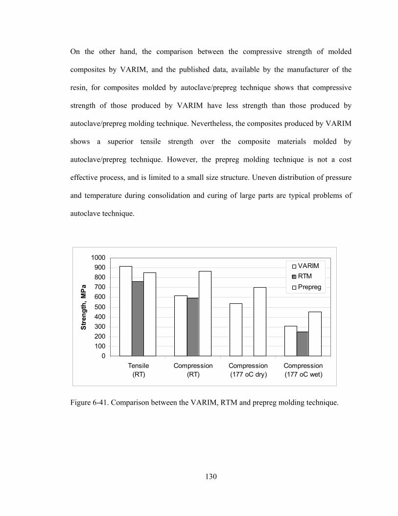
130

On the other hand, the comparison between the compressive strength of molded

composites by VARIM, and the published data, available by the manufacturer of the

resin, for composites molded by autoclave/prepreg technique shows that compressive

strength of those produced by VARIM have less strength than those produced by

autoclave/prepreg molding technique. Nevertheless, the composites produced by VARIM

shows a superior tensile strength over the composite materials molded by

autoclave/prepreg technique. However, the prepreg molding technique is not a cost

effective process, and is limited to a small size structure. Uneven distribution of pressure

and temperature during consolidation and curing of large parts are typical problems of

autoclave technique.

0100200300400500600700800900

1000

Tensile(RT)

Compression(RT)

Compression(177 oC dry)

Compression(177 oC wet)

Stre

ngth

, MPa

VARIMRTMPrepreg

Figure 6-41. Comparison between the VARIM, RTM and prepreg molding technique.

131

CHAPTER 7

CONCLUSIONS AND RECOMMENDATIONS

7.1 Introduction

This research focuses on an exploratory development of Vacuum Assisted Resin Infusion

Molding (VARIM) process for manufacturing high temperature polymer matrix

composites. The present study involves development of a comprehensive process virtual

model and a physical model to relate the process conditions to the evolved properties and

defects in vacuum assisted resin infusion molding of polymer composites. The virtual

model consists of three modules: resin infusion stage; resin cure stage; and cure

dependant mechanical properties. The physical model investigates the feasibility of

VARIM for fabricating high temperature polymer composites and the behavior of the

process with the change in its parameters. Characterization of properties, defects, and

internal structure of produced composites is the major thrust in this study.

The findings of this research will help in developing a science based technology for the

VARIM process for understanding of the process behavior and the effects of various

process parameters on the properties and integrity of the produced composites. The

numerical-experimental investigation provides capability for robust process and tooling

design, prediction, and characterization of process induced damage and properties of high

132

temperature polymer composites molded by VARIM. The developed virtual models

provide effective means for identifying process window for defects-free composite

structures with the desired properties.

7.2 Conclusions

From the results and discussion of this research, the following conclusions can be stated:

• With appropriate mold design based on the developed virtual model, sound

panels with high fiber volume fraction (58%) were successfully molded. Thus,

vacuum assisted resin infusion molding (VARIM) process was found to be

feasible for fabrication of high temperature polymer composites.

• The developed process (VARIM) is a closed one, offering an environmentally

benign manufacturing through the reduction of VOC emission.

• A virtual model for simulating the polymer flow behavior during the infusion

stage was developed and verified experimentally, with capabilities for

prediction of flow pattern, inside the mold, and evolved defects in vacuum

assisted resin infusion molding operation. This model is a useful tool for

process and mold design.

• A post processor visual mode involves combination of geometric

reconstruction scheme and graphic interchange format (GIF) was introduced

in the flow model in order to provide for effective visual presentation of the

results and to create a simple animation of the process.

133

• Several case studies using the developed model show the effect of race-

tracking on the formation of macro-voids and the importance of inlet ports

location and the proper ventilation for elimination of these defects.

• The process virtual model should help advance the manufacturing technology

for the production of affordable polymer composites for high temperature (up

to 250ºC) applications.

• The mechanical properties of panels produced by VARIM match the

properties obtained on a similar material system using other molding

techniques.

• The developed empirical relationship between VARIM process parameters,

within the range of the experimental design used in this study, and the evolved

properties helps in the determination of the optimum process window for the

required properties.

• The experimental investigation shows that post cure time and maximum cure

temperature are the most significant parameters in VARIM process for

manufacturing high temperature composites. Heating rate, with the range used

in the experimental design, has a little effect on VARIM process.

• This study shows that, within the range used for each parameter in the

experimental design, a maximum cure temperature of 183oC, a post cure time

of 5 hours, and a heating rate of 1.67oC/min are the optimum process

conditions for high-temperature and high-humidity applications. These curing

conditions would maximize the mechanical properties of composites molded

by VARIM.

134

• There is a very good agreement between the developed model predictions and

the experimental observations.

7.3 Recommendations

Based on the observations from the current research, the following recommendations are

suggested for future work:

• Construction of neural networks using the results obtained experimentally and

numerically, in the current research, in order to represent the relationships

between the process parameters and the evolved properties of the molded

composites by vacuum assisted resin infusion molding (VARIM) over a wider

range of process conditions.

• More complex shapes should be tested using VARIM process with multiple

resin inlets and vacuum ports.

• Numerical optimization techniques should be integrated with the developed

virtual models to define more global optimization process designs under given

constraints.

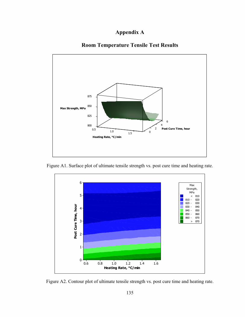
135

Appendix A

Room Temperature Tensile Test Results

64

Max Strength, MPa

800

825

850

875

2 Post Cure Time, hour0.51.0 01.5

Heating Rate, °C/min

Figure A1. Surface plot of ultimate tensile strength vs. post cure time and heating rate.

Heating Rate, °C/min

Post

Cur

e Ti

me,

hou

r

1.61.41.21.00.80.6

6

5

4

3

2

1

0

Max

820820 - 830830 - 840

Strength,

840 - 850850 - 860860 -

MPa

870> 870

< 810810 -

Figure A2. Contour plot of ultimate tensile strength vs. post cure time and heating rate.

136

64

Max Strength, MPa

800

840

880

920

2 Post Cure Time, hour180190 0200

Max Cure Tempraure, °C

Figure A3. Surface plot of tensile strength vs. post cure time and max cure temp.

Max Cure Tempraure, °C

Post

Cur

e Ti

me,

hou

r

204200196192188184

6

5

4

3

2

1

0

Max

840840 - 860860 - 880

Strength,

880 - 900900 - 920

> 920

MPa< 820

820 -

Figure A4. Contour plot of tensile strength vs. post cure time and max cure temp.

137

1.5

Max Strength, MPa

800

825

850

1.0

875

Heating Rate, °C/min180190 0.5200

Max Cure Tempraure, °C

Figure A5. Surface plot of ultimate tensile strength vs. post cure time and heating rate.

Max Cure Tempraure, °C

Hea

ting

Rat

e, °

C/m

in

204200196192188184

1.6

1.4

1.2

1.0

0.8

0.6

Max

820820 - 840840 - 860

Strength,

> 860

MPa< 800

800 -

Figure A6. Contour plot of ultimate tensile strength vs. max cure temp and heating rate.

138

64

Tensile Modulus, GPa

55.0

57.5

60.0

62.5

2 Post Cure Time, hour0.51.0 01.5

Heating Rate, °C/min

Figure A7. Surface plot of tensile modulus vs. post cure time and heating rate.

Heating Rate, °C/min

Post

Cur

e Ti

me,

hou

r

1.61.41.21.00.80.6

6

5

4

3

2

1

0

Tensile

57.257.2 - 58.458.4 - 59.6

Modulus,

59.6 - 60.860.8 - 62.062.0 -

GPa

63.2> 63.2

< 56.056.0 -

Figure A8. Contour plot of tensile modulus vs. post cure time and heating rate.

139

64

Tensile Modulus, GPa

56

60

64

2 Post Cure Time, hour180190 0200

Max Cure Tempraure, °C

Figure A9. Surface plot of tensile modulus vs. post cure time and max cure temp.

Max Cure Tempraure, °C

Post

Cur

e Ti

me,

hou

r

204200196192188184

6

5

4

3

2

1

0

Tensile

5858 - 5959 - 60

Modulus,

60 - 6161 - 6262 -

GPa

63> 63

< 5757 -

Figure A10. Contour plot of tensile modulus vs. post cure time and max cure temp.

140

1.5

Tensile Modulus, GPa

58

60

1.0

62

Heating Rate, °C/min180190 0.5200

Max Cure Tempraure, °C

Figure A11. Surface plot of tensile modulus vs. heating rate and max cure temp.

Max Cure Tempraure, °C

Hea

ting

Rat

e, °

C/m

in

204200196192188184

1.6

1.4

1.2

1.0

0.8

0.6

Tensile

58.658.6 - 59.259.2 - 59.8

Modulus,

59.8 - 60.460.4 - 61.061.0 -

GPa

61.6> 61.6

< 58.058.0 -

Figure A12. Contour plot of tensile modulus vs. heating rate and max cure temp.

141

Appendix B

Room Temperature Compressive Load Test Results

64

Comp Strength, MPa

480

510

540

570

2 Post Cure Time, hour0.51.0 01.5

Heating Rate, °C/min

Figure B1. Surface plot of compressive strength vs. post cure time and heating rate.

Heating Rate, °C/min

Post

Cur

e Ti

me,

hou

r

1.61.41.21.00.80.6

6

5

4

3

2

1

0

Max

- 500500 - 520520 - 540

Compressive

540 - 560560 - 580

>

Strength,

580

MPa< 480

480

Figure B2. Contour plot of compressive strength vs. post cure time and heating rate.

142

64

Comp Strength, MPa

450

500

550

2 Post Cure Time, hour180190 0200

Max Cure Tempraure, °C

Figure B3. Surface plot of compressive strength vs. post cure time and max cure temp.

Max Cure Tempraure, °C

Post

Cur

e Ti

me,

hou

r

204200196192188184

6

5

4

3

2

1

0

Max

- 460460 - 480480 - 500

Compressive

500 - 520520 - 540540

Strength,

- 560> 560

MPa< 440

440

Figure B4. Contour plot of compressive strength vs. post cure time and max cure temp.

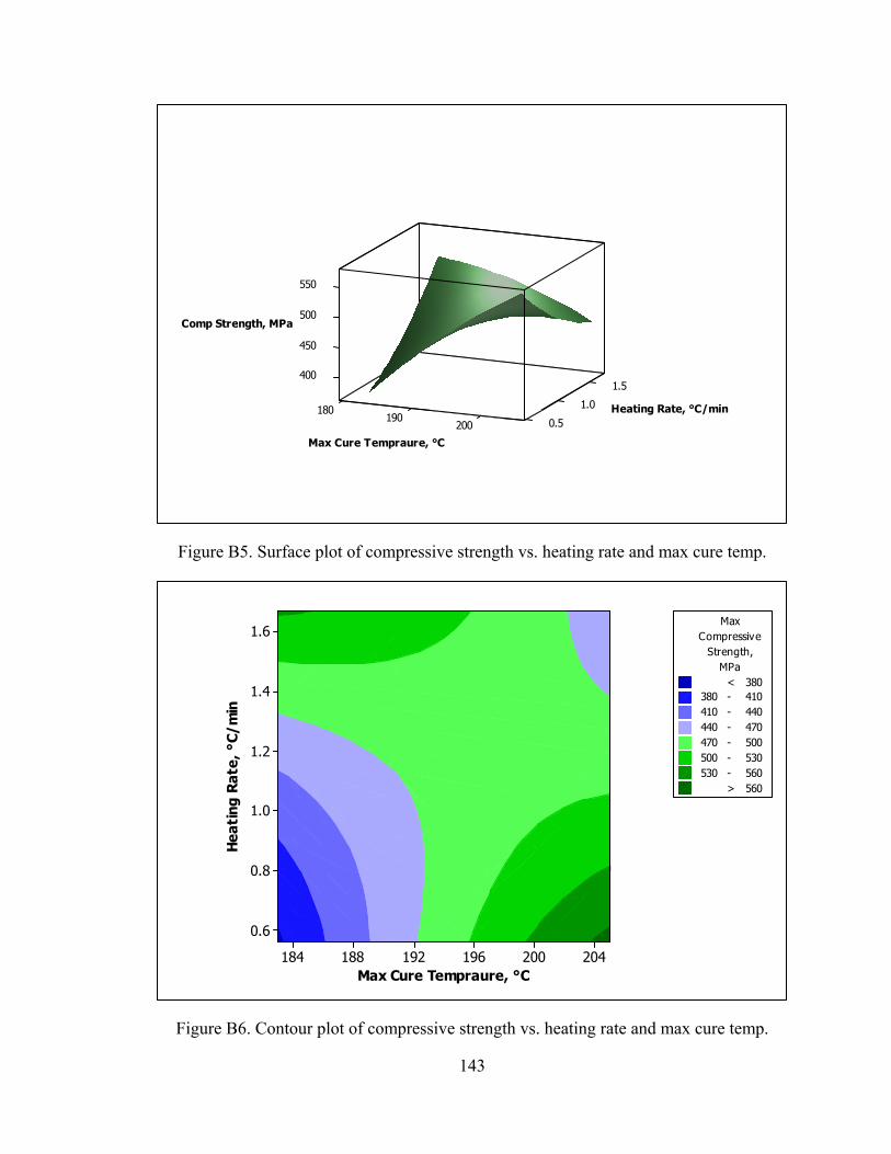
143

1.5

Comp Strength, MPa

400

450

500

1.0

550

Heating Rate, °C/min180190 0.5200

Max Cure Tempraure, °C

Figure B5. Surface plot of compressive strength vs. heating rate and max cure temp.

Max Cure Tempraure, °C

Hea

ting

Rat

e, °

C/m

in

204200196192188184

1.6

1.4

1.2

1.0

0.8

0.6

Max

- 410410 - 440440 - 470

Compressive

470 - 500500 - 530530

Strength,

- 560> 560

MPa< 380

380

Figure B6. Contour plot of compressive strength vs. heating rate and max cure temp.

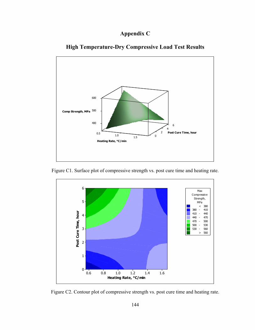
144

Appendix C

High Temperature-Dry Compressive Load Test Results

64

Comp Strength, MPa

400

500

600

2 Post Cure Time, hour0.51.0 01.5

Heating Rate, °C/min

Figure C1. Surface plot of compressive strength vs. post cure time and heating rate.

Heating Rate, °C/min

Post

Cur

e Ti

me,

hou

r

1.61.41.21.00.80.6

6

5

4

3

2

1

0

Max

- 410410 - 440440 - 470

Compressive

470 - 500500 - 530530

Strength,

- 560> 560

MPa< 380

380

Figure C2. Contour plot of compressive strength vs. post cure time and heating rate.

145

64

Comp Strength, MPa

300

400

500

600

2 Post Cure Time, hour180190 0200

Max Cure Tempraure, °C

Figure C3. Surface plot of compressive strength vs. post cure time and max cure temp.

Max Cure Tempraure, °C

Post

Cur

e Ti

me,

hou

r

204200196192188184

6

5

4

3

2

1

0

Max

- 400400 - 450450 - 500

Compressive

500 - 550550 - 600600

Strength,

- 650> 650

MPa< 350

350

Figure C4. Contour plot of compressive strength vs. post cure time and max cure temp.

146

1.5

Comp Strength, MPa

400

440

480

1.0

520

Heating Rate, °C/min180190 0.5200

Max Cure Tempraure, °C

Figure C5. Surface plot of compressive strength vs. post cure time and heating rate.

Max Cure Tempraure, °C

Hea

ting

Rat

e, °

C/m

in

204200196192188184

1.6

1.4

1.2

1.0

0.8

0.6

Max

- 430430 - 450450 - 470

Compressive

470 - 490490 - 510510

Strength,

- 530> 530

MPa< 410

410

Figure C6. Contour plot of compressive strength vs. max cure temp and heating rate.

147

64

Comp Modulus, GPa

60

61

62

63

2 Post Cure Time, hour0.51.0 01.5

Heating Rate, °C/min

Figure C7. Surface plot of compressive modulus vs. post cure time and heating rate.

Heating Rate, °C/min

Post

Cur

e Ti

me,

hou

r

1.61.41.21.00.80.6

6

5

4

3

2

1

0

Max

- 60.160.1 - 60.660.6 - 61.1

Compressive

61.1 - 61.661.6 - 62.162.1

Modulus,

- 62.6> 62.6

GPa< 59.6

59.6

Figure C8. Contour plot of compressive modulus vs. post cure time and heating rate.

148

64

Comp Modulus, GPa

60

64

68

2 Post Cure Time, hour180190 0200

Max Cure Tempraure, °C

Figure C9. Surface plot of compressive modulus vs. post cure time and max cure temp.

Max Cure Tempraure, °C

Post

Cur

e Ti

me,

hou

r

204200196192188184

6

5

4

3

2

1

0

Max

- 60.060.0 - 61.561.5 - 63.0

Compressive

63.0 - 64.564.5 - 66.066.0

Modulus,

- 67.5> 67.5

GPa< 58.5

58.5

Figure C10. Contour plot of compressive modulus vs. post cure time and max cure temp.

149

1.5

Comp Modulus, GPa

60

65

1.0

70

Heating Rate, °C/min180190 0.5200

Max Cure Tempraure, °C

Figure C11. Surface plot of compressive modulus vs. heating rate and max cure temp.

Max Cure Tempraure, °C

Hea

ting

Rat

e, °

C/m

in

204200196192188184

1.6

1.4

1.2

1.0

0.8

0.6

Max

- 5959 - 6161 - 63

Compressive

63 - 6565 - 6767

Modulus,

- 69> 69

GPa< 57

57

Figure C12. Contour plot of compressive modulus vs. heating rate and max cure temp.

150

Appendix D

High Temperature-Wet Compressive Load Test Results

64

Comp Strength, MPa

200

250

300

350

2 Post Cure Time, hour0.51.0 01.5

Heating Rate, °C/min

Figure D1. Surface plot of compressive strength vs. post cure time and heating rate.

Heating Rate, °C/min

Post

Cur

e Ti

me,

hou

r

1.61.41.21.00.80.6

6

5

4

3

2

1

0

Max

- 220220 - 240240 - 260

Compressive

260 - 280280 - 300300

Strength,

- 320> 320

MPa< 200

200

Figure D2. Contour plot of compressive strength vs. post cure time and heating rate.

151

64

Comp Strength, MPa

150

200

250

300

2 Post Cure Time, hour180190 0200

Max Cure Tempraure, °C

Figure D3. Surface plot of compressive strength vs. post cure time and max cure temp.

Max Cure Tempraure, °C

Post

Cur

e Ti

me,

hou

r

204200196192188184

6

5

4

3

2

1

0

Max

- 175175 - 200200 - 225

Compressive

225 - 250250 - 275275

Strength,

- 300> 300

MPa< 150

150

Figure D4. Contour plot of compressive strength vs. post cure time and max cure temp.

152

1.5

Comp Strength, MPa

250

300

1.0

350

Heating Rate, °C/min180190 0.5200

Max Cure Tempraure, °C

Figure D5. Surface plot of compressive strength vs. post cure time and heating rate.

Max Cure Tempraure, °C

Hea

ting

Rat

e, °

C/m

in

204200196192188184

1.6

1.4

1.2

1.0

0.8

0.6

Max

- 265265 - 280280 - 295

Compressive

295 - 310310 - 325325

Strength,

- 340> 340

MPa< 250

250

Figure D6. Contour plot of compressive strength vs. max cure temp and heating rate.

153

REFERENCES 1. Pike, T., McArthur, M., Schade, D., “Vacuum Assisted Resin Transfer Molding

of a Layered Structural Laminate for Application on Ground Combat Vehicles,” International SAMPLE Technical Conference, Vol. 28, 1996, pp.374-380.

2. Lewit, S., Jakubowski, J., “Low Cost VARTM Process for Commercial and

Military Applications,” International SAMPLE Symposium, Vol. 42, 1997, pp.1173-1187.

3. Lazarus, Paul, “Resin Infusion of Marine Composites,” International SAMPLE

Symposium, Vol. 41, 1996, pp.1447-1458. 4. Gillio, E, Advani, S.G., Fink, B.K., and Gillespie, J.W., “Investigation of the Role

of Transfer Flow in Co-injection Resin Transfer Molding,” Polymer Composites, Vol. 19, 1998, pp738-749.

5. Wu, T. and Hahn, T., “Mechanical Properties of E-Glass/Vinyl Ester Composite

Fabricated by VARTM,” International SAMPLE Symposium, Vol. 42, 1997, pp.1-12.

6. Heider, D., Hofmann, C., and Gillespie, Jr., “Automation and Control of Large –

Scale Composite Parts by VARTM Processing,” International SAMPLE Symposium, Vol. 45, 2000, pp.1567-1574.

7. Advani, S.G., and Sozer, E.M., “Process Modeling in Composite Manufacturing,”

Marcel Dekker, Inc., New York, NY, 2003.

8. Golestanian H., and El-Gizawy, A.S., “Modeling of Process Induced Residual Stresses in Thin Molded Composites with Woven Fiber Mats,” Journal of Composite Materials, Vol.35, No. 17, 2001, pp.1513-1528.

9. El-Gizawy, A. S., and Kuan, Yean-Der “Evolution and Management of Process-

induced Damage in Polymer Composites”, Proceedings, Global Symposium on Innovation in Materials Processing and Manufacturing, TMS Annual Meeting, New Orleans, Louisiana, February, 2001, pp.125-135.

10. Meador, M., “High Temperature Polymer-Matrix Composites”, In Flight Vehicle

Materials, Structure and Dynamics-Assessment and future Directions, Vol. 2, Ahmed Noor and Samuel Venneri, editors, American Society of Mechanical Engineers, 1994, pp.406-415.

11. Dillon, G., Mallon, P., and Monaghan, M., “The Autoclave Processing of

Composites” In Gutowski, T.G., editor, Advanced Composites Manufacturing, John Wiley and Sons, New York, NY, 1997.

154

12. Lee, L.J., “liquid Composite Modeling,” In Gutowski, T.G., editor, Advanced Composites Manufacturing, John Wiley and Sons, New York, NY, 1997.

13. A. H. Tullo, Chem. Eng. News, May 28, 2001, pp16.

14. Cycom 5250-4-RTM Resin System Description, Private Communication, Cytec

Fiberite, Inc., July, 2002.

15. Criss, J. and Koon, R., “High temperature VARTM of phenylethynyl terminated imide composites,” 33rd International SAMPE Technical Conference, 2001, pp1009-1021.

16. C. Williams, J. Summerscales, and S. Grove, “Resin infusion under flexible

tooling: a review,” Composites, 27A, 1996, pp 517-524.

17. Macro method, US patent No. 2495640, 1950.

18. W.H. Seemann, “Plastic transfer molding techniques for the production of fiber reinforced plastic structures,” US patent No. 4902215, 1989.

19. Trochu, F. Gauvin, R.Gao, D –M., “Numerical Analysis of the Resin Transfer

Molding Process by the Finite Element Method,” Advances in Polymer Technology. Vol. 12, No. 4, 1993, pp.329-342.

20. A. Hammami, R. Gauvin, and F. Trochu, “Modeling the edge effect in liquid

composites molding,” Composites, Part A 29A, 1198, pp 603-609.

21. Pillai, K.M. and Advani, S.G., “Numerical Simulation of Unsaturated Flow in Woven Fiber Performs During the Resin Transfer Molding Process,” Polymer Composites, Vol. 19, No. 1, Feb. 1998, pp.71-80.

22. Diallo, M.L., Gauvin, R., and Trochu, F., “Experimental Analysis and Simulation

of Flow through Multi-layer Fiber Reinforcements in Liquid Composite Molding”, Polymer Composites, vol. 19, No. 3, June 1998, PP.246-256.

23. Golestanian, H., and El-Gizawy, A.S., “Experimental and Numerical Modeling of

Mold Filling in Resin Transfer Molding,” Polymer Composites Journal, No.4, Vol. 19, August, 1998, pp. 359-406.

24. El-Gizawy, A.S., and Kuan, Year-Dear, “Numerical Characterization of Mold

Injection in Resin Transfer Molding Process,” Advances in Polymer Technology, Vol. 19, No. 3, Septemeber 2000, pp.173-179.

25. Hsiao, Kuang-Ting., Gillespie and Avani, S.G., “Numerical Simulation of

Unsaturated Flow in Woven Fiber Performs During the Resin Transfer Molding Process,” Polymer Composites, Vol. 19, No. 1, Feb. 1998, pp.71-80.

155

26. Kang, M.K., Lee, W.I., and Hahn, “Analysis of Vacuum Bag resin Transfer

Molding Process,” Composites, Part A: Applied Science and Manufacturing, Vol. 32, 2002, pp.1553-1560.

27. S. Jiang, C. Zhang, and B. Wang, “Optimum arrangement of gate and vent for

RTM process design using a mesh distance based approach,” Composites: part A33, 2002, pp 471-481.

28. B. Kim, G. J. Nam, and J. W. Lee, “Optimization of filling process in RTM using

a genetic algorithm and experimental design method,” Polymer composites, Vol. 23, No. 1, Feb,. 2002, pp 72-86.

29. A. Gokce, K.T. Hsiao, and S. G. Advani, “Branch and bound search optimization

injection gate locations in liquid composite molding processes,” Composites: part A33, 2002, pp 1263-1272.

30. B. Miaie, Y.F. Chen, and A.M. Mescher, “A methodology to obtain a desired

filling patter during resin transfer molding,” Journal of composite materials, Vol. 36, No. 14, 2002, pp 1677-1692.

31. Jun H. Choi and C.K.H. Dharan, “Mold fill time and void reduction in resin

transfer molding achieved by articulated tooling,” Journal of composite materials, Vol. 36, No. 19, 2002, pp 2267-2285.

32. Jun H. Choi and C.K.H. Dharan, “Enhancement of resin transfer molding using

articulated tooling,” Polymer composites, Vol. 23, No. 4, August 2002, pp 674-681.

33. P. de Luca, Y. Benoit, and J. Trochon, “Coupled pre-forming/injection

simulations of liquid composite molding progresses,” 47th International SAMPLE symposium, 2002, pp 1307-1316.

34. L. Joubaud, and F. Trochu, “Simulation of the manufacturing of an ambulance

roof vacuum assisted resin infusion (VARI),” Composites-2002, Composites fabricators association, 2002.

35. Adel Hammami, “Key factors affecting permeability measurement in the vacuum

infusion molding process,” Polymer composites, Vol. 23, No. 6, 2002, pp 1057-1067.

36. White, S. R. and Hahn, H.T., “Process Modeling of Composite Materials:

Residual Stress Development During Cure. Part I. Model Formulation,” Journal of Composite Materials, vol. 26, No. 16, 1992, pp.2402-2422.

156

37. White, S. R. and Hahn, H.T., “Process Modeling of Composite Materials: Residual Stress Development During Cure. Part II. Experimental Validation,” Journal of Composite Materials, vol. 26, No. 16, 1992, pp.2423-2453.

38. White, S. R. and Hahn, H.T., “Cure Cycle Optimization for Reduction of

Processing-Induced Residual Stresses in Composite Materials,” Journal of Composite Materials, vol. 27, No. 14, 1993, pp.1352-1378.

39. Golestanian, H., and El-Gizawy, A.S., “Cure Dependent Lamina Stiffness

Matrices of Resin Transfer Molded Composite Parts,” Journal of Composite Materials, No. 23, Vol. 31, 1997, pp.2402-2423.

40. Osswald, Tim A., Sun, Esther M., and Tseng, Shi-Chang, “Experimental

Verification on Simulation Shrinkage and Warpage of Thin Compression Molded SMC Parts,” Polymers & Polymer Composites, Vol. 2, No. 3, 1994, pp. 187A-198A.

41. Bogetti, Travis A. and Gillespie, John W. Jr., “Process-Induced Stress and

Deformation in Thick-Section Thermosetting Composite Laminates,” Journal of Composite Materials, Vol. 26, No. 5, 1992, pp.626-658.

42. Tseng, Shi-Chang and Osswald, Tim, A., “Prediction of Shrinkage and Warpage

of Fiber Reinforced Thermoset Composite Parts,” Journal of Reinforced Plastics and Composites, Vol. 13, 1994, pp.698-721.

43. Loos.A.C., Sayer, J., McGrane, R., and Grimsley, B., “VARTM Process Model

Development,” International SAMPLE Symposium, Vol. 461, 2001, pp. 1049-1060.

44. Y.K. Kim and I.M. Daniel, “Cure cycle effect on composite structures

manufactured by resin transfer molding,” Composite materials, Vol. 36, No. 14, 2002, pp 1725-1743.

45. Dillon, G., Mallon, P., and Monaghan, M.: Advanced Composites Manufacturing,

John Wiley and Sons, New York, NY, 1997.

46. Meyers, R.H., Montgomery, D.C., “Response Surface Methodology: Process and Product Optimization Using Designed Experiments,” John Wiley and Sons, New York, Ny, 1995.

47. Y. Luo, I. Verpoest, K. Hoes, M. Vanheule, H. Sol, and A. Cardon, “Permeability

measurement of textile reinforcements with several test fluids,” Composites-part A: applied science and manufacturing, v32, 2001, pp 1497-1504.

48. D. L. Youngs, “Time Dependant Multi Material Flow Distortion,” In K. W.

Morton and M. J. Baines, Academic Press, 1982.

157

49. Srinivasan, R., Wang, T., and Lee, L., “Chemorheology of High Temperature

RTM Resins,” 53rd Society of Plastics Engineers, ANTEC Technical Conference, 1995, pp3016-3029.

50. Ito, Makoto, and Chou, Tsu-Wei, “An Analytical and Experimental Study of

Strength and Failure Behavior of Plain Weave Composites,” Journal of Composite Materials, Vol. 32, No. 1, 1998, pp.2-30.

51. Jones, Robert M., “Mechanics of Composite Materials,” Taylor & Francis,

Philadelphia, PA, 1999, pp. 151-157.

52. Kaw, K., “Mechanics of Composite Materials,” CRC Press, New York, 1997, pp.174-178.

53. Patanakar, S. V., “Numerical Heat Transfer and Fluid Flow,” McGraw-Hill, New

York, 1980, pp.59-61.

54. Product data sheet of Magnamite AS4 Carbon Fiber, provided by Hexcel Schwebel, 2005.

55. Li, Chao, “Experimental and Analytical Investigation of Failure Behavior in

Satin-Weave Composites and Uni-Weave Satin-Weave Hybrid Composites,” Dissertation, Texas A&M University, 2001.

56. Loos, C., and Springer, S., “Moisture Absorption of Graphite-Epoxy Composites

Immersed in Liquid and in Humid Air,” Journal of Composite Materials, v13, 1979, pp.131-147.

57. Collings, T.A., “The Effect of Observed Climatic Conditions on the moisture

Equilibrium Level of Fiber-Reinforced Plastics,” Composites, Jan 1986, pp.33-41.

58. Shen, Chi, and Springer, S. “Moisture Absorption and Desorption of Composite Materials,” Journal of Composite Materials, v10, 1976, pp.2-20.

59. Lincoln, E., and Morgan, J., Shin, E., “Moisture Absorption-Network Structure

Correlations in BMPM/DABPA Bismaleimide Composite Matrices,” Journal of Advanced Materials, v32, No. 4, 2000, pp.24-34.

60. Springer, S., and Tang, Jian-Mao, “Accelerated Environmental Testing of

Composites,” Journal of Composite Materials, v21, 1987, pp.225-242.

61. Ju, J. and Morgan, R.J., “Characterization of Microcrack Development in BMI-Carbon Fiber Composite under stress and Thermal Cycling,” Journal of Composite Materials, v38, 2004, pp. 2007-2024.

158

62. He, Y., Zhong, Y. and Zhou, J., “Post-Curing Effects on Physical and Mechanical Properties of IM7/5250-4 Composites,” 30th International SAMPE Technical Conference, 1998, pp. 226-233.

63. Antony, Jiju, “Design of Experiments for Engineers and Scientists,” Butterworth-

Heinmann, Burlington, MA, 2003.

64. Montogomery, C., “Introduction to Statistical Quality Control,” John Wiley & Sons, New York, 1996.

65. Hodgkinson, J.M>, “Mechanical Testing of Advanced Fiber Composites,”

Woodhead Publishing Limited, Cambridge, England, 2000.

66. Adams, D.F. and Welsh, J.S., “The Wyoming Combined Loading Compression Test Method,” Journal of Composites Technology abd Research, JCTRER, 19(3), 197, pp. 123-133.

67. Li, R.B., “Moisture Absorption and Hygrothermal Aging in a Bismaleimide Resin

and its Carbon Fiber Composites,” Dissertation, Univ. of Michigan, 2001.

68. Wright, W.W., “The Effect of Diffusion of Water into Epoxy Resins and their Carbon-Fiber Reinforced Composites,” Composites, July 1981, pp.201-205.

69. Biney, O. and Zhong, Y., “Hudrolytic Effects on the Properties of Graphite/BMI

Composites,” 43rd International SAMPE Symposium, 1998, pp.120-129.

70. Biney, O. and Wilson, E., “Hygrothermal Effects on the Thermal and Mechanical Properties of IM7/5250-4 Composites,” 44th International SAMPE Symposium, 1999, pp.734-740.

71. Zhong, Yang, and He, Yu, “Short-Term ging effects on Thermal and Mechanical

Properties of IM7/5250-4 Composites,” 44th International SAMPE Symposium, 1999, pp.741-747.

72. Bechel, T., and Fredin, B., “Combined Cryogenic and Elevated temperature

cycling of Carbon/polymer Composites,” 47th International SAMPE Symposium, 2002, pp.808-819.

73. Morgan, J., and Ju, Jaehyung, “Characterization of BMI-Carbon Fiber Composite

Microcrack Development Under Thermal Cycling,” Society of Plastics Engineers, ANTEC Technical Conference, 2003, pp.2059-2063.

74. Walker, Sandra, “Thermal Effects on the Compressive Behavior of IM7/PETI5

Laminates,” Journal of Composites Materials, v38, No. 2, 2004, pp.149-162.

159

VITA

Ahmed Khattab was born on November 27, 1966 in Alexandria, Egypt. He received his

B.S. degree in Mechanical Engineering form Faculty of Engineering-Alexandria

University, Egypt in 1990. He joined CATERPILLAR Inc. dealer in Egypt for one year

as a Maintenance Engineer. Then he worked as a Researcher for nine years at the

Research Center of Arab Academy for Science and Technology, Alexandria-Egypt. He

earned his Master degree in Mechanical Engineering form Faculty of Engineering-

Alexandria University, Egypt in 1998.

In summer 2000, he went to the United States of America to pursue his Ph.D. from

University of Missouri-Columbia. Ahmed is married to Eman Matter and he is a father of

two boys, Karim and Khaled.