2

3

Explorations in Phenomenology as Practiced in Waldorf Schools

A Science News Roundletter Editor: David Mitchell

1158 Quince Ave.Boulder, CO 80304

Phone and Fax: 303/ 541-9244E-mail: davidm@awsna.org

© Copyright 2011 by AWSNA Publications

All materials may be reproduced for individual use in Waldorf/Steiner Schools but not published without permission of the editor.

Printed with the Support of the Waldorf Curriculum Fund____________________________________________________________________________________________________________ VOL. 17, #27 Spring 2011

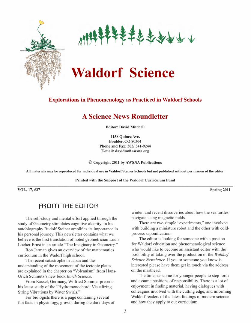
FROM THE EDITOR

The self-study and mental effort applied through the study of Geometry stimulates cognitive alacrity. In his autobiography Rudolf Steiner amplifies its importance in his personal journey. This newsletter contains what we believe is the first translation of noted geometrician Louis Locher-Ernst in an article “The Imaginary in Geometry.”

Ron Jarman gives an overview of the mathematics curriculum in the Wadorf high school.

The recent catastrophe in Japan and the understanding of the movement of the tectonic plates are explained in the chapter on “Volcanism” from Hans-Urich Schmutz’s new book Earth Science.

From Kassel, Germany, Wilfried Sommer presents his latest study of the “Hydromonochord: Visualizing String Vibrations by Water Swirls.”

For biologists there is a page containing several fun facts in physiology, growth during the dark days of

winter, and recent discoveries about how the sea turtles navigate using magnetic fields.

There are two simple “experiments,” one involved with building a miniature robot and the other with cold-process saponification.

The editor is looking for someone with a passion for Waldorf education and phenomenological science who would like to become an assistant editor with the possibility of taking over the production of the Waldorf Science Newsletter. If you or someone you know is interested please have them get in touch via the address on the masthead.

The time has come for younger people to step forth and assume positions of responsibility. There is a lot of enjoyment in finding material, having dialogues with colleagues involved with the cutting edge, and informing Waldorf readers of the latest findings of modern science and how they apply to our curriculum.

Waldorf Science

4

Books of Interest

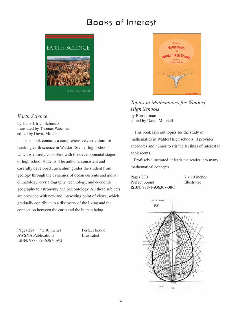
Earth Scienceby Hans-Ulrich Schmutztranslated by Thomas Wassmeredited by David Mitchell

This book contains a comprehensive curriculum for teaching earth science in Waldorf/Steiner high schools which is entirely consistent with the developmental stages of high school students. The author’s consistent and carefully developed curriculum guides the student from geology through the dynamics of ocean currents and global climatology, crystallography, technology, and economic geography to astronomy and paleontology. All these subjects are provided with new and interesting point of views, which gradually contribute to a discovery of the living and the connection between the earth and the human being.

Pages 224 7 x 10 inches Perfect bound AWSNA Publications IllustratedISBN: 978-1-936367-09-2

Topics in Mathematics for Waldorf High Schools by Ron Jarmanedited by David Mitchell

This book lays out topics for the study of mathematics in Waldorf high schools. It provides anecdotes and humor to stir the feelings of interest in adolescents.

Profusely illustrated, it leads the reader into many mathematical concepts.

Pages 230 7 x 10 inches Perfect bound IllustratedISBN: 978-1-936367-08-5

5

Topics in Mathematics for Waldorf High Schools—11th Gradeedited by Robert Neumann

The series Mathematics for the High School was specifically designed with math teachers in mind. Not only are the books useful resources for gaining familiarity with teaching approaches used in a Waldorf school, but they are also a source of inspiration – offering fresh perspectives and new insights – for courses that have perhaps been taught many times. This book contains experienced teachers’ suggestions for lesson blocks covering topics taught in the 11th grade in the Waldorf curriculum.

Themes include:

• Analytical Geometry• Projective Geometry• Spherical Geometry• Sequences and Limits

The emphasis is on projective geometry, since this topic is not very familiar to most teachers.

The material is not only described theoretically, but includes many examples, exercises and “hands-on” hints for the lessons. Some information about the historical background of the major themes rounds out many of the contributions.

Pages 288 7.25 x 9 inches Softcover Illustrated AWSNA PublicationsISBN 978-1-936367-11-5

Research Bulletin Spring/Summer 2010Volume XV, Number 1

• What Can Rudolf Steiner’s Words to the First Waldorf Teachers Tell Us Today?

• Social Emotional Intelligence: The Basis for a New Vision of Education in the United States

• Rudolf Steiner’s Research Methods for Teachers• Combined Grades in Waldorf Schools: Creating

Classrooms Teachers Can Feel Good About• Educating Gifted Students in Waldorf Schools• How Do Teachers Learn with Teachers?• Does Our Educational System Contribute to

Attentional and Learning Difficulties in Our Children?• Survey on Waldorf School Trustee Education

Also included are the work of the Research Fellows and reports on current projects.

Pages 72 7.5 x 11 inches AWSNA Publications Softcover

6

Colloquium on High School Physics

Organized by the Waldorf High School Research Group through the Research Institute for Waldorf Education.A group of experienced teachers discusses and explores the Waldorf physics curriculum and suggest new ideas while solving some of the riddles found in the current curriculum.

AWSNA Publications 8.5 x 11 inchesPages 98 Spiralbound Illustrated

Associative EconomicsSpiritual Activity for the Common Good

This comprehensive book guides the reader to substantially rethink aspects of economic life. It opens doors for new perspectives, describes pitfalls and successes, and gives practical small steps one can take in order to effect change and improve the human condition.

AWSNA Publications 5.5 x 8.5 inchesPages 164 IllustratedISBN: 978-1-936367-10-8 Perfect bound

1

Waldorf Journal Project #17March 2011

AWSNA

From Images to Thinking

Compiled and edited by

David Mitchell

Happiness is a butterfly, which when pursued, is always just beyond your grasp, but which, if you will sit down quietly, may alight upon you. – Nathaniel Hawthorne

Waldorf Journal Project #17From Images to thInkIngEdited by David Mitchell

Contents

• Children Learn in Images by Rosemary Wermbter

• The Fairy Tale of the Crystal Ball by Christianne Brown

• Interpreting Fairy Tales by Rudolf Steiner

• How to Create, Tell, and Recall a Story by Rudolf Steiner

• The Secret of Children’s Pictures by Armin Krenz

• Research into Resilience by Christof Wieckert

• Resilient Children: First Food or Fast Food

by Katherine Train

• Why Waldorf Works: From a Neuroscientific Perspective

by Dr. Regalena Melrose

• The Senses by Eileen M. Hutchins

• The Training of Observation by Eileen M. Hutchins

• Observation and Thinking by Eileen M. Hutchins

• The Activity of Thinking by Eileen M. Hutchins

• An Education for Our Time by Christof Wieckert

• A Bold Step Forward by Andreas Neider

• Internet Crutch by Mathias Maurer

Pages 116 8.5 x 11 inches Spiralbound Illustrated

Available at cost through AWSNA Publications and gratis Online at www.waldorflibrary.org.

7

The Leafcutter Antsby Edward O. Wilson and Bert Hölldobler

Leafcutter ants are familiar to all those who live in rural Texas and Louisiana. These are the ants busily running in columns on trails they keep free of debris and vegetation, carrying freshly-cut sections of leaves and flower petals over their heads like umbrellas. If one followed the ants to their nest, one would discover an immense network of tunnels, the majority of which are an underground garden in which the ants grow their food—fungus planted onto a substrate of chewed plant material previously brought by the ants. As readers we are introduced to earth’s most evolved animal society. With the colony’s queen as its reproductive organ, the various ages and types of workers as the brain, heart, and other organs; and the communication among the ants similar to the communication of nerves and ganglia, a leafcutter ant colony can be truly considered as a superorganism.

Pages 160 6.1 x 8.2 inches SoftcoverW. W. Norton & Company IllustratedISBN: 978-0393338683

Research Bulletin, Autumn/Winter 2010, Volume XV Number 2

Contents:

• The Inner Life and Work of the Teacher

• The Human Body as a Resonance Organ: A Sketch of an Anthropology of the Senses

• Aesthetic Knowledge as a Source for the Main Lesson

• The Work of Emmi Pikler

• Knitting It All Together: Handwork and Spacial Dynamics

• Seven Myths of Social Participation of Waldorf Graduates

• Volunteerism, Communication, Social Interaction: A Survey of Waldorf School Parents

• A Timeline for the Association of Waldorf Schools of North America

Also included are the work of the Research Fellows and reports on current projects.

Pages 81 7.5 x 11 inches Perfect bound cover Illustrated

8

For Teachers

Points to Consider in Teaching Science

1. Did I arouse the interest of the students?

2. Was there “soul breathing” in the class? Did they laugh and also feel deep introspection? (A lesson without a laugh is a lost opportunity.)

3. What real images were brought as opposed to judgments or pre-formed concepts?

4. Were different senses of the students properly stimulated?

5. Was the experiment clear and phenomenological?

6. Was the recapitulation without equipment successful?

7. Was a concept arrived at by the class?

8. Did I prepare the students properly for the night? Were the questions that arose from the morning lesson stimulating? Did they give back through the will today what went through the senses yesterday?

9. What new skill or knowledge did the students receive today?

10. Was every student acknowledged, and did they each produce effort?

11. What was done to get the students moving in some way?

12. How can I better apply all of the above to tomorrow’s lesson?

– DSM

9

A BRIEF OVERVIEWOF THE WALDORF HIGH SCHOOL

MATHEMATICS CURRICULUM

by

Ron Jarman

In high school work it is the activity of thinking which becomes the soul captain’s principal lieutenant in the third phase of growing up. “Thinking,” said Rudolf Steiner, “is the all-one being which permeates everything.” There are four stages in the development and strengthening of the activity of thinking and they correspond to the path running through classes (or grades) 9, 10, 11 and 12. Nevertheless all three parts of soul activity develop strongly during this later phase from age fourteen upwards. As the teenager’s own soul penetrates his bodily activities, he has to experience and overcome an inner soul chaos as he learns to look in a new way at everything in the world and in himself.

In mathematics as well as in other subjects, the ninth grader wants to experience everything afresh. He welcomes the change from having a class teacher to being taught each subject by someone who has worked to become an expert in it, assisted by the rigors of a university degree and life experience. Teachers in their twenties and thirties are often the best people to teach young people of high school age. The ninth grader wants to be shown anew how to do addition sums and long divisions for example, but now in a fully conscious way, grasping the reasons for each whim of written layout. No longer is the underlying aim to receive the teacher’s tick at the end of one’s calculations. The pupil wants to be able to know himself whether or not his answers are correct. The authority of the individual teacher is replaced by experience of and guidance by the truth itself. Despite the obvious lies, half-truths, deceptions and hypocrisies in the world and in the young person’s immediate environment, he wants above all to find those realms where he can assert and experience that the world is true. As a young child he needed assurance that the world is fundamentally good. Between roughly 7 and 14 he needed confirmation that the world is beautiful. Already basically strengthened in will and feeling respectively, he now needs this third guarantee to help him find the earthly home for his own personality.

In Class 9 the emphasis a teacher can lay is on contrasts. Awareness of contrasts leads to the consciousness in which

10

thinking can grow. In art lessons the best medium is black (charcoal sticks or paint brushes) on white paper. The physics of electromagnetism will contrast the power unit of an electric train with that of the telephone earpiece. The principle is the same in both, but the contrast in current is enormous.

The first could be described as allopathic electricity and the second as homeopathic electricity. Contrasts in other subjects are between drama and comedy, plate tectonics and volcanoes, Olympic gymnastics and country dancing. At the same time there are strong common elements. In mathematics there is the contrast between melody and harmony in music. In geometry the conic sections ellipse and hyperbola are contrasted, and comparison can be made between these and the respective form and function relationship between head and limbs. In addition there is the intermediate chest and rhythmic system, represented by the parabola, so that the metamorphosis in both groups can be made apparent.

In Class 10, pairs of contrasts and their interactions carries the thinking awareness a stage further. Ancient history in this class culminates in a careful study of Greek civilization and the Socratic dialogues. The Pythagorean-Platonic description of the four elements in terms of the two contrasts moist-dry and warm-cold is part of this, and much of the mathematics developed from this can be used. Geometric constructions of the four basic spirals (Archimedean, Equiangular, Reciprocal and Asymptotic Circle) illustrate the four progressions of numbers arising therefrom, and how they indicate a progression from material to noetic aspects of the world. It is independent judgment that evolves in Class 10. Perhaps the prime example of this is in trigonometry. To be able to stand far away from a mountain, take three measurements and then be able to calculate the mountain’s height without becoming involved in climbing it exemplifies the particular ingredient of human intelligence required to make an objective judgment unfettered by personal feelings of involvement—which would be difficult for Class Niners to achieve.

By Class 11 the students are ready to plunge into greater detail in everything they study, whether it be the history of music (one of the main lessons they have), the story of Parzival and its significance, atomic theory, the theory of organic cellular structure, or computer technology. It is the year when analysis is the key word. So in mathematics differential calculus is introduced—the same kind of procedure towards smaller and finally infinitesimal parts is required to do this. Also in geometry the fundamental theorem of Projective Geometry is proved and made use of. At the same time the principle of duality shows how the importance of point-like entities must be complemented by the equally valid and important planar entities which structure and shape the plant and organic world as a whole. The intellect can become finely honed at this age as well as developing an awareness of the noetic dimensions of life.

11

The final school year (Class 12) gives the students an opportunity to gather together the many results obtained through analysis and experience and discover the higher unities as true progenitors. Intellect has prepared the ground for reason. Analysis gives way to synthesis. The many points of view which scientific and artistic work have revealed help to form the indispensable modesty and wonder which every student requires in beginning to build his own view of the nature of both the world in which he lives and what being human really means. He becomes aware that he possesses a unique individuality and that it will suffer rust and tarnishing if he allows it to become infused with mere egotism. He will seek a higher synthesis of himself with the best that human society endeavors to achieve. So in physics Class 12 concentrates on understanding the whole world of color. The diverging scientific descriptions of Newton, Goethe, Ostwald and others have to be evaluated and their contributions to the whole subject synthesized, yet not fully determined—only adult life will provide the experiences needed to do that. Renaissance and modern painting, which together with architecture figure in another main lesson, will further nourish such endeavors.

Class 12 mathematics is again concerned with synthesis. Differential calculus gives rise to integral calculus. Human reason can now grasp chaos theory and fractals. Earthly geometry (what used to be called Euclidean geometry) is seen to be but a limited part of a Projective Euclidean (or parabolic) geometry, which is only one of a whole host of geometries, e.g., hyperbolic, elliptic and polar Euclidean geometries, all of which have their own forms of measurement, be it of distance or angle. Practice in working with money in three different ways back in Class 6 now grows into a deep study of economics; and the realization dawns in Class 12 that the problems of world economy will never be solved until a far more holistic approach to them is made than the world has so far managed to evolve.

It is important in upper classes just as in lower classes that every student gain a clear impression of what the topics introduced contribute to the whole curriculum of school subjects as well as to the whole mathematics curriculum. The difference in difficulty of problems set for more able and less able students will be become much greater by Class 12. Nonetheless the social value of keeping all students of the same chronological age in the same main lesson block is far reaching. The whole class will experience together the basic qualities of the various topics and their relevance to a wide range of human activities in life—all this in perhaps the initial half hour each day. Then the individual work of students and group work of some of them will follow different directions, some manual, practical and artistic, others of an advanced mathematical, analytical and also synthesizing character.

12

Some Fun Facts of Physiology

HEART & BLOODThe heart is a hollow muscle which weighs

between 8–12 ounces.The heart beats 104,000 times every day.The blood makes more than 1,000 circuits/ day.Every day 1,000,000 (one million) blood cells

are produced in your body.

LUNGSWe breathe 23,000 times a day.The surface area of your lungs is 1,000 square

feet. This is 20 times greater than the surface of your skin.

EYESThe eye blinks 17,000 times per day; this would

total 30 minutes if all at once.We move our eye muscles 2,000,000 times per

day.The eye can distinguish 8 million differences in

color (hues).Your eye and brain can build color from waves

of energy.

EARSYour ear can distinguish more than 300,000

tones.

NERVESNerve impulses travel at the rate of 350 feet/

second.Every night we move 40–70 times during sleep.

MUSCLES If all 600 muscles in your body pulled in one

direction, you could lift 25 tons.The tongue is the strongest muscle for its size

in the body, The gluteus maximus (rear end) is the biggest.

DIGESTIONYour digestive tract is 30 feet long.

HAIRIn the average lifetime your hair will grow 25

feet.We lose 45 scalp hairs every day.

BONESThe body has 206 different bones; more than half

of these are in your hands and feet.The human skull is made up of 29 different bones.One cubic inch of bone can withstand a two-ton

force.The foot has 26 bones, 107 ligaments, 19 muscles,

all of which interact in an intricate manner.The interior of the spine looks like melted icicles.

It has two distinct areas which allow the bones to be both light and strong: (1). the dense, ivory-like outside and (2) the airy, canal-like interior.

SKINEvery day we shed 14.4 million dead skin

particles (keratin).A square centimeter of skin has 100 sweat

glands, 12 feet of nerves with 100 nerve endings, 10 hair follicles, 15 sebaceous glands, and 3 feet of blood vessels.

The skin has 2 million pores to rid the body of water, salt, and other wastes. We eliminate 500 grams of waste products every day. This creates body odor.

Every pound of excess fat requires 200 miles of capillaries to support it.

When we shiver we involuntarily warm our body.

– DSM

13

THE IMAGINARY IN GEOMETRY

by Louis Locher-Ernst

translated by Paul Courtney

provided via Ernst Schuberth and Mikko Bojarsky

1. IntroductionImaginary objects can be visualized by means of real pictures in various

fundamentally different ways. The usual representation of the complex number z = x + iy in rectangular (x, y) or Riemannian spherical co-ordinates is specially suitable for a graphical representation of the region that an analytic function w = f (z) assigns to some domain of the independent variable z. Useful though this representation is in many investigations, it nevertheless leaves the geometer dissatisfied in one respect. The ∞2 complex points of a line, e.g. the points x = a + ia´ (a, a´ real) of the x-axis, are symbolized by the real points of a plane, and as a result the non-real points of the line appear detached from this as their base. Suppose we want to pursue geometry in the plane including the complex elements. If we hold fast to the accepted function-theoretic representation, then in order to accommodate the real pictures of the complex points of the lines concerned, we would have to assign a separate plane to every line of the plane.

Von Staudt1 famously discovered a real representation of the complex elements of space (point, line and plane) corresponding directly to the essence of the thing.The reason why a completely natural handling of this representation is still relatively unknown is probably due to the fact that the von Staudt theory is usually developed purely projectively right from the start. Of course the projective theory of involutions is at the heart of the matter. Yet for an introduction it may be asked whether, with a more hands-on mental picturing of involutions, we cannot accommodate the power of intuition. What follows2 should show that this is at least possible. In order to assume a minimum of prior knowledge we shall use metric concepts at the outset. Our aim with regard to isotropic lines, imaginary conic sections, imaginary tangents, generating a sphere as a ruled surface, etc., is to achieve a concreteness which means more than a purely schematic picture, which can of course be obtained in many different ways. In the first Part we restrict ourselves in the main to the complex elements of a real plane. In the second Part the essentially more intricate relationships in space are described. We are trying above all to find intuitive pictures and just to sketch the proofs sufficiently for those who are interested.

2. The arrow of an imaginary pointFirst we introduce the key concept we shall be working with throughout.The points of a line g may be combined in pairs A,A1 and B,B1 and C,C1 etc. in such

a way that for a certain fixed point M of g and an arbitrary pair P, P1 the relationship exists.

14

MP ·MP1 = k = constant (1)

Such a pairing is called an involution3; M is the center, k the power of the involution. The point corresponding to the center M according to (1) is the point at infinity of g.

In doing this the segments MP, MP1 are regarded as having the same sign whenever the directions from M to P and from M to P1 are the same. Thus if the power k is positive then the segments MP, MP1 of every pair have the same direction, if k is negative, the opposite direction. Suppose we choose on the line g the zero- and unit-point of a co-ordinate system, and a, x, x1 are the co-ordinates of M, P and P1. Then the involution is determined by the relation (x − a)(x1 − a) = k (a, k real). If k is positive the involution is called hyperbolic, if negative elliptic. If k = 0, the involution is a “degenerate” one, in which every pair of corresponding points includes the center.

We call to mind some properties of an involution which follow easily from the definition:

Through projection, every involution is transformed into an involution of the same kind.

An involution is determined by two pairs A, A1 and B, B1 of corresponding points. In an elliptic involution two pairs of corresponding points separate each other. If A, A1 is a pair of corresponding points of an elliptic involution, there is just one pair B, B1 of this involution that separates A, A1 harmonically. The construction of B, B1 for a given A we give later.4

A non-degenerate involution contains just two double points, that is, two points that correspond to themselves. Indeed the equation (x − a)(x − a) = k has the two solutions x = a ± √ k . The double points are real for a hyperbolic, complex for an elliptic involution. In both cases every pair P, P1 of corresponding points separates the double points harmonically.

Suppose P moves through the point-range in a certain sense. Then in an elliptic involution the corresponding point P1 moves through the range in the same sense, but in a hyperbolic involution in the opposite sense. The double points of a hyperbolic involution can be understood as the meeting points of this reciprocal movement. In an elliptic involution the corresponding points P, P1 do not meet each other in real points. Yet the elliptic involution unambiguously determines two imaginary5 points as double points. If P moves through the point-range in a certain sense, then an elliptic involution relates to this movement of P a movement in the same sense of the corresponding point P1.

We regard this co-ordinated movement as the real picture of an imaginary double point; the other imaginary double point is given by the co-ordinated movement in the opposite sense. In short, a directed elliptic involution represents an imaginary point, and conversely every imaginary point of the line in question can be given by a directed elliptic involution n.

These co-ordinated movements are essential for a vivid intuition of the imaginary. The movements cannot be captured in a single geometrical picture however, so we introduce a symbol that unambiguously determines these movements (that is, the directed elliptic involution). We give the center M of the involution and one of the two principal points P1 N1 . These are the two corresponding points that are equidistant from M. If this distance is h and M has the co-ordinate a, then the equation of the elliptic involution is

(x − a)(x1 − a) = −h2 (2)

15

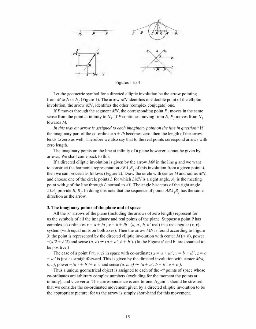
Figures 1 to 4

Let the geometric symbol for a directed elliptic involution be the arrow pointing from M to N or N1 (Figure 1). The arrow MN identifies one double point of the elliptic involution, the arrow MN1 identifies the other (complex conjugate) one.

If P moves through the segment MN, the corresponding point P1 moves in the same sense from the point at infinity to N1. If P continues moving from N, P1 moves from N1 towards M.

In this way an arrow is assigned to each imaginary point on the line in question.6 If the imaginary part of the co-ordinate a + ih becomes zero, then the length of the arrow tends to zero as well. Therefore we also say that to the real points correspond arrows with zero length.

The imaginary points on the line at infinity of a plane however cannot be given by arrows. We shall come back to this.

If a directed elliptic involution is given by the arrow MN in the line g and we want to construct the harmonic representation ABA1B1 of this involution from a given point A, then we can proceed as follows (Figure 2): Draw the circle with center M and radius MN, and choose one of the circle points L for which LMN is a right angle. A1 is the meeting point with g of the line through L normal to AL. The angle bisectors of the right angle ALA1 provide B, B1. In doing this note that the sequence of points ABA1B1 has the same direction as the arrow.

3. The imaginary points of the plane and of spaceAll the ∞4 arrows of the plane (including the arrows of zero length) represent for

us the symbols of all the imaginary and real points of the plane. Suppose a point P has complex co-ordinates x = a + ia´, y = b + ib´ (a, a´, b, b´ real) in a rectangular (x, y)-system (with equal units on both axes). Then the arrow MN is found according to Figure 3: the point is represented by the directed elliptic involution with center M (a, b), power −(a´2 + b´2) and sense (a, b) ➛ (a + a´, b + b´). (In the Figure a´ and b´ are assumed to be positive.)

The case of a point P(x, y, z) in space with co-ordinates x = a + ia´, y = b + ib´, z = c + ic´ is just as straightforward. This is given by the directed involution with center M(a, b, c), power −(a´2 + b´2+ c´2) and sense (a, b, c) ➛ (a + a´, b + b´, c + c´).

Thus a unique geometrical object is assigned to each of the ∞6 points of space whose co-ordinates are arbitrary complex numbers (excluding for the moment the points at infinity), and vice versa: The correspondence is one-to-one. Again it should be stressed that we consider the co-ordinated movement given by a directed elliptic involution to be the appropriate picture; for us the arrow is simply short-hand for this movement.

16

4. The lines of a planeSuppose there is a directed elliptic involution (given, say, by an arrow) in a line l. If

we project its points from any point S lying outside l, then we determine in the pencil (S) a directed elliptic line involution. A distinguished elliptic line involution in (S) is the right-angled involution which relates to each line in S, the line in S that is normal to it. There is no need to explain what the harmonic representation aba1b1 of a directed elliptic line involution means.

The duality principle in the plane shows it is correct to state: A directed elliptic line involution is the picture of an imaginary line. Since there are also imaginary lines in space which are not given in this way, we call the imaginary lines just introduced special imaginary lines.7 That there exists a one-one correspondence between the imaginary lines of the plane and the directed elliptic line involutions will be a consequence of what follows.

The imaginary point P(ABA1B1) lies in the real line g if the elements of the involution ABA1B1, that is, the arrow of P8, lies in g. Hence just one real line goes through an imaginary point (in the plane). The imaginary point P(ABA1B1) lies in the imaginary line g(aba1b1) if the point and line involutions representing them—including their senses—are perspective. In an imaginary line there is just one real point, namely the base point S of the directed elliptic involution representing the line.

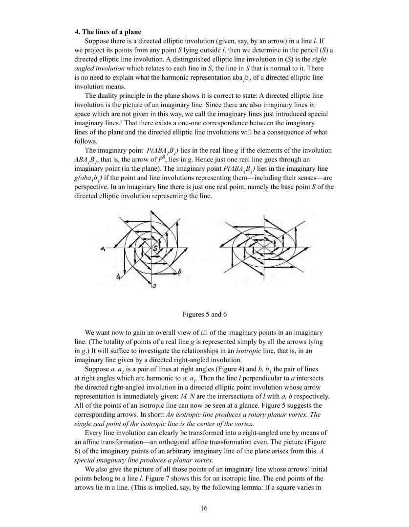
Figures 5 and 6

We want now to gain an overall view of all of the imaginary points in an imaginary line. (The totality of points of a real line g is represented simply by all the arrows lying in g.) It will suffice to investigate the relationships in an isotropic line, that is, in an imaginary line given by a directed right-angled involution.

Suppose a, a1 is a pair of lines at right angles (Figure 4) and b, b1 the pair of lines at right angles which are harmonic to a, a1. Then the line l perpendicular to a intersects the directed right-angled involution in a directed elliptic point involution whose arrow representation is immediately given: M, N are the intersections of l with a, b respectively. All of the points of an isotropic line can now be seen at a glance. Figure 5 suggests the corresponding arrows. In short: An isotropic line produces a rotary planar vortex. The single real point of the isotropic line is the center of the vortex.

Every line involution can clearly be transformed into a right-angled one by means of an affine transformation—an orthogonal affine transformation even. The picture (Figure 6) of the imaginary points of an arbitrary imaginary line of the plane arises from this. A special imaginary line produces a planar vortex.

We also give the picture of all those points of an imaginary line whose arrows’ initial points belong to a line l. Figure 7 shows this for an isotropic line. The end points of the arrows lie in a line. (This is implied, say, by the following lemma: If a square varies in

17

such a way that one corner S is fixed and a corner adjacent to S describes a line, then the other two corners also describe lines.) By affine transformation it now follows that:

If the initial points of the arrows representing points of a special imaginary line g belong to a line l, then the end points form a point range similar to the range of initial points.

If two points P, Q (that is, their arrows) of a special imaginary line are given, then, using this proposition, further points of the line can easily be constructed (Figure 8).

Figures 7 to 10

We call two arrows connected if the end point of one arrow is the initial point of the other. The distinctive positioning of two connected arrows in relation to the base S (to the real point) will prove to be useful. Figure 9 shows two such arrows 12, 23 belonging to an isotropic line (that is, representing points of this line). The construction (given in Figure 10) of the base S of the line of which two connected arrows 12, 23 are given follows by affine transformation: 1234 and 124S are parallelograms.

Finally Figure 11 shows those arrows of a special imaginary line which lie in the real lines of a pencil T. (In the Figure the line is assumed to be isotropic; the general case follows by affine transformation.)

A special case should also be mentioned: A directed elliptic line involution in a pencil of parallel lines gives a special imaginary line with base S at infinity. The initial points of all the arrows of this line are in that line a of the pencil which is related in the involution to the line at infinity, the end points are in a line b whose corresponding line b1 is the same distance from a as b (Figure 12).

The positioning of the arrows given by the points of an imaginary line, explained above, can easily be deduced analytically from the equation Ax + By + Cz = 0, where A, B, C are arbitrary complex coefficients.

Figures 11 and 12

18

If we intersect a directed elliptic line involution with the line at infinity of the plane, the resulting section is a directed elliptic point involution determining an imaginary point of this line.

5. Connecting and intersecting in the plane

A. Two points P, Q determine exactly one line g, which contains P and Q.B. Two lines p, q determine exactly one point G, which lies on p and q.

Proof of A: If P, Q are real there is nothing to prove. If P is real and Q imaginary, then g is imaginary, provided P does not belong to the line of the arrow Q. P is the base of the line involution which represents g and which is perspective to the involution of Q.

If P, Q are imaginary then g is imaginary provided P, Q do not belong to the same real line. g must be represented by the directed elliptic line involution which, including sense, is perspective to the directed point involutions representing P and Q respectively. Let U be the point of intersection (Figure 13) of the lines of the arrows P, Q. We determine the harmonic representations UV U1V1, UV’U’1V'1 (according to Figure 2) of the involutions representing P, Q. As a result the connecting lines U1U’1 = u1, V V’ = v, V1V’01 = v1 go through a point S. The lines u = SU, u1, v, v1 determine the directed elliptic line involution uvu1v1 that represents the line g we seek.

A simpler construction is the one given in Figure 14 using the remark made earlier about connected arrows. First construct the connected arrows 12, 23 from the arrows P, Q, whereby 12 belongs to the line through the initial points, 23 to the line through the end points of the arrows P, Q. This is easily done using the proposition relating to Figure 8.

Figures 13 and 14

Proof of B: We immediately consider the case in which p, q are imaginary and have distinct real centers S, S’. Let u be the connecting line SS'. Then we determine (using a section in a line, say) the harmonic representations uvu1v1, uv’u’

1v’1 of the line involutions

giving p, q. V = vv’, V1 = v1v’1, U1 = u1u’

1 then lie in a real line g. If U is the point of intersection ug, then the directed involution UV U1V1 provides the required point of intersection G.

This gives us control of the operations of connecting and intersecting in the complex geometry of the plane. How continuity is understood in the complex domain is immediately clear from continuity in the corresponding domain of arrows. It is not possible here to go into detail about ordering axioms.

6. The imaginary points and tangents of a conic sectionWe give the constructions and suggest the proofs afterwards. Figure 15a shows the

situation for a circle. Construct a concentric rectangular hyperbola with major axis the same length as the circle’s diameter. The half-chords perpendicular to the major axis

19

provide arrows (with points on the hyperbola) which all represent imaginary points of the circle. The tangent in the imaginary point P is given as follows: Determine the pole S of the line s containing the arrow P. The directed line involution in S perspective to the point involution representing P gives the tangent. To obtain all the points of the circle we must rotate Figure 15a about the circle’s center. Especially noteworthy is the following. From the circle’s field of arrows, it is seen immediately that every circle contains two particular imaginary points of the line at infinity, namely those points in which the directed right-angled involutions (isotropic lines) intersect that line. To send tangents to the circle from one of its inner points S, we must determine a planar vortex with center S, that has one arrow in common with the circle. The arrow field of the circle enables us to perceive directly that the tangents from the center of the circle are the isotropic lines of this point.

Figures 15 a, b, c

If we let the circle’s radius tend to zero, its arrow field is transformed into a double rotary vortex (Figure 15b, the two isotropic lines of the center). Figure 15c shows the points of an imaginary circle.

To construct the imaginary points and tangents of an arbitrary real conic section, we introduce the concept of harmonic reflection. Given a point A which does not lie on the line t, the harmonic reflection of a figure UVW . . . in A and t means the central collineation with center A, axis t and characteristic -1. Thus to construct the reflection U1 of U, we must intersect the line AU with t and determine the point U1 which, with U, separates point A and that point of intersection harmonically.

Suppose now any conic k is given. We want to determine its points of intersection with a set of parallel (real) lines. Let s be a line of the set (Figure 16) that does not meet k in real points. First construct a tangent t parallel to s, let B be its point of contact, A the second end-point of the diameter through B. Now reflect k harmonically in A and t. A conic section k1 is formed which touches k in A and B. AB cuts s in the initial point C of the arrows CU1 and CV1 whose end points belong to k1. These arrows represent the imaginary points of intersection P,Q of s with k.

If we carry out the construction for all lines which do not intersect k in real points, we obtain all of the imaginary points of k. (If k is a parabola, k1 is a parabola congruent to k.)

To construct the tangent in point P, determine the pole S of the line s through the arrow P. The directed elliptic line involution in S that is perspective to the involution representing P supplies the required tangent.

The proof of the construction given follows from the proposition:9 The extra triangle of a complete 4-point inscribed in a conic section is a polar triangle. Hence, if in Figure 17 XY rotates about the point S, the extra points X’, Y’ of the complete 4-point ABXY describe the polar line s of S; moreover X’, Y’ are conjugate, and thus describe the point involution produced on s by k.10 The points U1, V1 in Figure 16 are those corresponding points of this involution which separate their mid-point C and the point at infinity of s harmonically.

20

Figures 16 and 17

We now have an intuitive overview of all the imaginary points and tangents of a real conic section. It is a simple matter to carry this over to the purely imaginary conic sections as well. But in what follows we shall turn to the imaginary elements in space.

7. Imaginary planesAn imaginary point of space is given by a directed elliptic point involution, which

we represent by an arrow.11 A special imaginary line has as picture a directed elliptic line involution. The duality principle in space tells us how we have to define an imaginary plane. The form dual to a point-range is a plane-sheaf. If we connect the base line p of the sheaf with the points of a point-range, whose base line is skew to p, an involution in the range is transferred to the sheaf. The picture of an imaginary plane π is a directed elliptic plane involution.

Figures 18 and 19

A point P lies in the plane π if either P (thus also its arrow) belongs to the real base p of π or the plane involution representing π, including the sense of the involution, is perspective to the directed involution representing P (Figure 18). In an imaginary plane there is exactly one real line, namely the base p of the involution furnishing the plane.

A special imaginary line g lies in the imaginary plane π if the involution representing g, including the involution’s sense, is perspective to the involution representing π (Figure 19).

We need to get an overview of all of the ∞4 points of an imaginary plane π. Apart from the real and imaginary points of the base p of π, they are those imaginary points whose involutions, including their sense, are perspective to the involution that represents π. On each real line distinct from p there lies exactly one point of π. To visualize the corresponding set of arrows, it is enough to do this for a plane π given by a directed right-

21

angled plane involution αβαβ since the general case can be obtained from this by an affine transformation.

Suppose point M in a is the center of a line-pencil (M) whose plane is parallel to α1 (Figure 20), hence normal to α. The directed point involutions cut out of the lines of pencil (M) by the directed right-angled plane involution all have M as their center. The points of intersection with one of the planes β bisecting the angle between α and α1 are related to the corresponding points of intersection with the other bisecting plane β1. The single exception is the line of pencil (M) parallel to p, which meets π in the real point at infinity of p. Hence the line of intersection l of the plane β with the plane of pencil (M) contains the end-points of the arrows representing the points of intersection of pencil (M) with π, while M is their common initial point.

Figures 20 and 21

All the arrows of π not lying in p (that is, arrows representing the points of the plane π) are given if the half-pencil of arrows indicated in Figure 20 is translated in the direction of p, rotated about p, and expanded away from p. Hence normal projection onto a plane normal to p produces a rotary vortex representing the line of intersection of π with the plane of projection.

In the general case we obtain, instead of the coaxial circular cylinders of Figure 20, elliptical cylinders which are coaxial, similar and similarly situated.

Note also the special case when the base line p of the plane involution is at infinity. In this case the set of initial points and the set of end-points of the arrows of π each fill a plane (Figure 21, in which α1 is the plane at infinity).

There are now the questions of intersecting two arbitrary planes and connecting two arbitrary points of space. We take first the special case where the real base lines of the two planes or of the two points intersect.

Two points P, Q whose arrow lines intersect lie in the connecting plane of these lines. It was shown in Section 5 that two such points determine one and only one connecting line which is easy to construct.

Dual to this: Two planes π, κ whose bases p, q intersect, determine a unique line which lies in both planes.

If π, κ are both real there is nothing to prove. Suppose π is real and κ imaginary. Then the section in π of the plane involution of κ is a directed elliptic line involution which represents the line of intersection, which is thus a special imaginary line. Only in

22

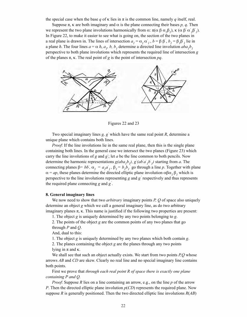
the special case when the base q of κ lies in π is the common line, namely q itself, real.Suppose π, κ are both imaginary and α is the plane connecting their bases p, q. Then

we represent the two plane involutions harmonically from α: π(α β α1β1), κ (α β’ α

’1β’

1). In Figure 22, to make it easier to see what is going on, the section of the two planes in a real plane is drawn in. The lines of intersection a1 = α1 α

’1 , b = β β’, b1 = β1β’

1 lie in a plane δ. The four lines a = α δ, a1, b, b1 determine a directed line involution aba1b1 perspective to both plane involutions which represents the required line of intersection g of the planes π, κ. The real point of g is the point of intersection pq.

Figures 22 and 23

Two special imaginary lines g, g’ which have the same real point R, determine a unique plane which contains both lines.

Proof: If the line involutions lie in the same real plane, then this is the single plane containing both lines. In the general case we intersect the two planes (Figure 23) which carry the line involutions of g and g’; let a be the line common to both pencils. Now determine the harmonic representations g(aba1b1), g’(ab’a’

1b’1) starting from a. The

connecting planes β= bb’, α1 = a1a’1 , β1 = b1b1

’ go through a line p. Together with plane α = ap, these planes determine the directed elliptic plane involution αβα1 β1 which is perspective to the line involutions representing g and g’ respectively and thus represents the required plane connecting g and g’.

8. General imaginary linesWe now need to show that two arbitrary imaginary points P, Q of space also uniquely

determine an object g which we call a general imaginary line, as do two arbitrary imaginary planes π, κ. This name is justified if the following two properties are present:

1. The object g is uniquely determined by any two points belonging to g.2. The points of the object g are the common points of any two planes that gothrough P and Q.And, dual to this:1. The object g is uniquely determined by any two planes which both contain g.2. The planes containing the object g are the planes through any two pointslying in π and κ.We shall see that such an object actually exists. We start from two points P,Q whose

arrows AB and CD are skew. Clearly no real line and no special imaginary line contains both points.

First we prove that through each real point R of space there is exactly one plane containing P and Q.

Proof: Suppose R lies on a line containing an arrow, e.g., on the line p of the arrow P. Then the directed elliptic plane involution p(CD) represents the required plane. Now suppose R is generally positioned. Then the two directed elliptic line involutions R(AB)

23

and R(CD) determine two special imaginary lines with the common real point R. By the proposition proved at the end of Section 7, these lines determine a unique connecting plane. This contains the points P and Q.

This is how we shall proceed further. We shall put through P and Q two specially chosen planes δ and ε. Then we shall investigate the object that consists of the common points of these two planes. Finally we shall show that this object possesses both of the required properties 1 and 2 given above. As a result we shall have produced a perfectly clear picture of the general imaginary line.

The line AC, through the two initial points of the arrows P and Q, and the line BD, which is skew to AC, through their end-points, uniquely determine two parallel planes α and β, α through AC and β through BD (Figure 24). Let u be the line of intersection at infinity of these planes α, β. The involutions that represent P and Q determine in sheaf (u) the same directed elliptic involution αβα1β1. In this involution the plane at infinity of space α1 corresponds to plane α, the plane β1 the same distance from α as β, corresponds to plane β. The imaginary plane δ determined by the involution αβα1β1 is one of the two distinguished planes though P and Q mentioned.

To determine the second distinguished plane ε through P and Q we project the arrows P, Q normally onto plane α. The projections P’

Q’ are two arrows A B’

and C D’ , that

is, two imaginary points in α which determine a planar vortex, a special imaginary line g’

in α. Let H be the real point of g’ , that is, the center of the planar vortex.

The line h perpendicular to α then determines, together with the directed elliptic line involution representing g’, a directed elliptic plane involution, that is, a plane ε, which by construction goes through P and Q.

Figures 24 and 25

The points common to both planes δ and ε can now be seen at a glance. Let the totality of these points be called (W). We have to determine the arrows common to two arrow-manifolds of the type indicated in Figures 20 and 21.

All the arrows of δ begin in α and end in β. Of these arrows we have to pick out those belonging to ε. Each of α’s actual points is the initial point of exactly one such arrow, whose normal projection onto α belongs to the line g’. Therefore the object (W) arises as follows: We leave the initial points of all the arrows of the planar vortex of g’ unchanged, but we raise their end-points at right angles to α through the fixed length f, namely the distance between planes α, β.

In Figure 25 we imagine first that g’, the normal projection of the object (W) onto α, produces a rotary vortex (Figure 26). The general case follows by means of an orthogonal affine transformation.

If we also add to each arrow of (W) the arrow which gives the conjugate complex point, then the latter arrow’s end-point lies in the plane β1. The lines which carry the arrows of (W) can thus be constructed as follows. Draw in β and β1 two circles of the

24

same size whose centers N, N1 lie in the “axis” h and connect those points of these circles that lie one above the other; the connecting lines are the rulings of a circular cylinder. Next the circle in β must be rotated round N through an angle of 90º. The circular cylinder becomes a hyperboloid of revolution. Doing this for all circles in β with center N and adding the line at infinity u gives us all of the lines which carry arrows of the object (W). The arrows begin in α and end in β. We call the object (W) a spatial vortex (Figure 27). In the case we had in mind first we have a rotary spatial vortex. The general spatial vortex arises from the latter by means of an orthogonal affinity. The spatial vortex (W) uniquely determined by two generally positioned imaginary points P,Q in space represents the general imaginary line g through P, Q. Such a line contains no real point and lies in no real plane.

Figures 26 and 27

We see immediately that (W) possesses Property 1. Any two arrows of (W) determine the planes α and β in exactly the same way as P and Q do, and their normal projections onto α determine, by construction, the same line g’. We shall show that the second property is also present. First we reflect that there are ∞8 general imaginary lines: The shape of the vortex is determined by one quantity, say by the eccentricity of the “cross-sectional ellipse” (Figure 27). The “size” of the vortex is determined by the length f of the principal arrow HN. The position of the vortex in space is determined by six parameters: four parameters for the position of axis h, one parameter for the position of the principal plane α perpendicular to h, and one for the cross-sectional ellipse’s major axis. If the length f tends to zero, the limiting object that results is a special imaginary line.

We turn our attention now to the set of lines that carries arrows of the vortex. It follows immediately from the construction that exactly one such line passes through each real point of space. Furthermore each real plane of space contains exactly one such line, which follows from the reflection that every real plane intersects the planes δ and ε in one line each, whose point of intersection provides one arrow of the vortex, which arrow lies in that real plane. The set of arrow lines is thus a linear congruence of lines. The totality of real lines meeting two real skew lines m and n also has the property that generally exactly one line of this totality goes through each real point and exactly one such line lies in each real plane. The only exceptions are the points and planes of the two focal lines m, n. This totality is called a hyperbolic congruence, the totality of arrow lines of a spatial vortex is an elliptic congruence. Whereas the former determines two real focal lines, the latter determines a pair of conjugate complex, general imaginary lines g, g*. Because if we replace each arrow of (W) by its conjugate, that is, by the arrow with the opposite direction, the same length and the same initial point, the result is clearly another spatial vortex (W*). The elliptic congruence determines precisely the two vortices (W*) and

25

(W*). (The two planes β, β1, which are symmetric with respect to the central point H and normal to the axis h, contain those points which are twisted through 90º with respect to each other.)

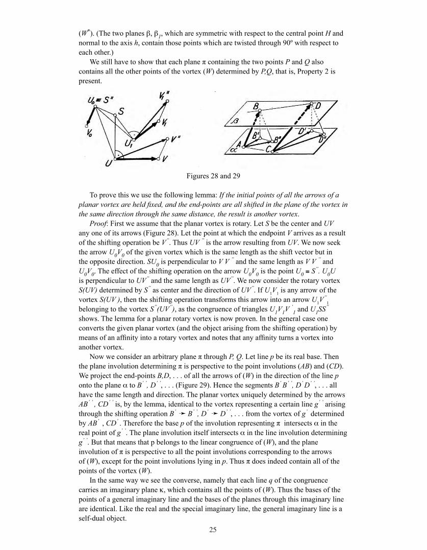
We still have to show that each plane π containing the two points P and Q also contains all the other points of the vortex (W) determined by P,Q, that is, Property 2 is present.

Figures 28 and 29

To prove this we use the following lemma: If the initial points of all the arrows of a planar vortex are held fixed, and the end-points are all shifted in the plane of the vortex in the same direction through the same distance, the result is another vortex.

Proof: First we assume that the planar vortex is rotary. Let S be the center and UV any one of its arrows (Figure 28). Let the point at which the endpoint V arrives as a result of the shifting operation be V’’. Thus UV ’’ is the arrow resulting from UV. We now seek the arrow U0V0 of the given vortex which is the same length as the shift vector but in the opposite direction. SU0 is perpendicular to V V ’’ and the same length as V V ’’ and U0V0. The effect of the shifting operation on the arrow U0V0 is the point U0 ≡ S’’. U0U is perpendicular to UV’’ and the same length as UV’’. We now consider the rotary vortex S(UV) determined by S’’ as center and the direction of UV’’. If U1V1 is any arrow of the vortex S(UV ), then the shifting operation transforms this arrow into an arrow U1V

’’1

belonging to the vortex S’’(UV’’), as the congruence of triangles U1V1V ’1 and U1SS’’

shows. The lemma for a planar rotary vortex is now proven. In the general case one converts the given planar vortex (and the object arising from the shifting operation) by means of an affinity into a rotary vortex and notes that any affinity turns a vortex into another vortex.

Now we consider an arbitrary plane π through P, Q. Let line p be its real base. Then the plane involution determining π is perspective to the point involutions (AB) and (CD). We project the end-points B,D, . . . of all the arrows of (W) in the direction of the line p onto the plane α to B’

’, D’

’, . . . (Figure 29). Hence the segments B’

B’ ’, D’

D’ ’, . . . all

have the same length and direction. The planar vortex uniquely determined by the arrows AB’

’ , CD’

’ is, by the lemma, identical to the vortex representing a certain line g’

’ arising

through the shifting operation B’ ➛ B’

’, D’

➛ D’ ’, . . . from the vortex of g’

determined by AB’

, CD’ . Therefore the base p of the involution representing π intersects α in the

real point of g’ ’. The plane involution itself intersects α in the line involution determining

g’ ’. But that means that p belongs to the linear congruence of (W), and the plane

involution of π is perspective to all the point involutions corresponding to the arrows of (W), except for the point involutions lying in p. Thus π does indeed contain all of the points of the vortex (W).

In the same way we see the converse, namely that each line q of the congruence carries an imaginary plane κ, which contains all the points of (W). Thus the bases of the points of a general imaginary line and the bases of the planes through this imaginary line are identical. Like the real and the special imaginary line, the general imaginary line is a self-dual object.

26

We have now reached one of the main goals of our remarks: to gain a correct picture of the general imaginary line in the most elementary way possible.

9. ConclusionTo elaborate complex synthetic geometry further is not be possible here. We shall

merely add some remarks. It is easy to see that all further propositions about connecting and intersecting the elements point, line and plane are generally valid: A plane and a line not belonging to it have just one point in common; three points not lying in the same line determine just one plane that contains them; and so on.

Also the imaginary elements contained in, for example, a second degree surface can now be represented in a concrete and vivid way. In an oval second degree surface there lie two families of special imaginary lines, but no real and no general imaginary lines. The hyperboloid of one sheet carries, apart from two families of real lines, general imaginary lines as well. Figure 30 shows the situation with a sphere, all of whose points we want to see together at a glance. A plane α1 through its center intersects it in a great circle whose arrow field is shown in the Figure (cf. page 8).

If the intersecting plane is shifted to the tangent plane α3, the result is the arrow field of two conjugate isotropic lines. In position α4 the only points the plane still has in common with the sphere are the imaginary points of an imaginary circle. (To obtain all of the points of a particular cross-sectional object, we must of course rotate Figure 30 about axis a.)

Figures 30

There is also the question of how the normal representation of the complex numbers in a rectangular (x, y)-system fits into the general theory of the imaginary in geometry. To answer this let I be that imaginary point of the line at infinity which is the section in that line of every directed right-angled line involution in the (x, y)-plane with positive sense. If we connect I with all points of the x-axis then the real point of the line connecting I with the point x = a+ia’ of the x-axis clearly has co-ordinates x = a, y = a’.

Hopefully our explanations have shown that the arrow representation used here has some advantages, at least in the linear and quadratic domains.

27

Sphere and hyperboloid of one sheet

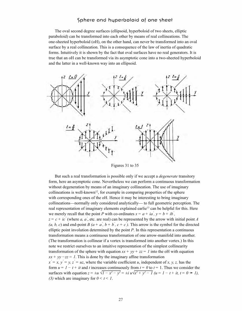
The oval second degree surfaces (ellipsoid, hyperboloid of two sheets, elliptic paraboloid) can be transformed into each other by means of real collineations. The one-sheeted hyperboloid (oH), on the other hand, can never be transformed into an oval surface by a real collineation. This is a consequence of the law of inertia of quadratic forms. Intuitively it is shown by the fact that oval surfaces have no real generators. It is true that an oH can be transformed via its asymptotic cone into a two-sheeted hyperboloid and the latter in a well-known way into an ellipsoid.

Figures 31 to 35

But such a real transformation is possible only if we accept a degenerate transitory form, here an asymptotic cone. Nevertheless we can perform a continuous transformation without degeneration by means of an imaginary collineation. The use of imaginary collineations is well-known12, for example in comparing properties of the sphere with corresponding ones of the oH. Hence it may be interesting to bring imaginary collineations—normally only considered analytically— to full geometric perception. The real representation of imaginary elements explained earlie13 can be helpful for this. Here we merely recall that the point P with co-ordinates x = a + ia’, y = b + ib’, z = c + ic’ (where a, a’, etc. are real) can be represented by the arrow with initial point A (a, b, c) and end-point B (a + a’, b + b’, c + c’). This arrow is the symbol for the directed elliptic point involution determined by the point P. In this representation a continuous transformation means a continuous transformation of one arrow-manifold into another. (The transformation is collinear if a vortex is transformed into another vortex.) In this note we restrict ourselves to an intuitive representation of the simplest collinearity transformation of the sphere with equation xx + yy + zz = 1 into the oH with equation xx + yy −zz = 1. This is done by the imaginary affine transformation x’ = x, y’ = y, z’ = uz, where the variable coefficient u, independent of x, y, z, has the form u = 1 − t + it and t increases continuously from t = 0 to t = 1. Thus we consider the surfaces with equation z = ±u √1 − x2 − y2 = ±i u√x2 + y2 − 1 (u = 1 − t + it, t = 0 ➛ 1), (3) which are imaginary for 0 < t < 1.

28

Figures 36 to 40

For t = 0 (1) represents a sphere, for t = 1 an oH. Figures 31 to 35 show the transition in the section with the (y, z)-plane (x = 0). In these the z-arrows are only indicated for real y. The stages t = 0, 1/4, 1/2, 3/4, 1 are drawn. The real points (degenerate arrows) of the circle (t = 0) become arrows of increasing length, the end-points remaining on the initial circle, the initial points eventually moving as far as the y-axis. The arrows representing the imaginary points, for real y, of the circle (t = 0)—these arrows’ lengths (which are the amounts of their imaginary parts) diminish, while the initial points of the arrows move downwards or upwards from the y-axis as far as the rectangular hyperbola whose real points are the final stage of the transition. (The points of the section of the surface (1) in the (x, y)-plane—a circle—remain unchanged.)

The sphere possesses two sets of ∞2 imaginary generators (special imaginary lines), while the oH carries, apart from ∞2 general imaginary lines, in particular also two sets of ∞1 real generators. Figures 35 to 40 indicate how these come about with our affine transformation of the sphere. They arise from those generators (rotary vortices) of the sphere whose real points lie in the (x, y)-plane. The other generators of the sphere are transformed into general imaginary lines of the oH.

29

Resources(* Asterisked note was added by Mikko Bojarsky.)

1. G.K. Christian von Staudt, Contributions to the Geometry of Position [Beiträge zur Geometrie der Lage], Nürnberg 1856, No. 1.

2. This account is a concise summary of part of a course of lectures on elementary mathematics from a higher standpoint.

3. This curious name was coined by G. Desargues in his paper “Rough draft of an attempt to deal with the outcome of the meeting of a cone with a plane” [Brouillon projet d’une atteinte aux événements des rencontres d’un cone avec un plan], Paris, 1639. Regarding this the translator M. Zacharias (Oswald Klassiker, No. 197), says “The word involution means the state of being curled up as happens in the youthful stage of parts of a shoot.”

4. For the involutions that arise as sections of a complete 4-point or a pencil of circles, and so forth refer, e.g., to the always excellent work by Theodore Reye, The Geometry of Position [Die Geometrie der Lage], Vol. 1, 5th edition, Leipzig, 1909.

5. It is usual to speak of imaginary (rather than complex) points even when the co-ordinate is not purely imaginary.

6. In the book Plane Analytic Curves and Their Associated Depictions [Ebene analytische Kurven und zu ihnen gehőrige Abbildungen], Leipzig and Berlin, 1911, E. Study uses in plane geometry a pair of real points to represent an imaginary point, e.g., in terms of the above, the pair N,N1. For the historical development, cf. A. Ramorino The Imaginary Elements in Geometry [Gli elementi imaginari nella geometrie], Giornale die Matematiche 35, p. 242, 1897.

7. A representation of the imaginary line corresponding to the arrow is made possible by distinguishing one point of the plane (just as the arrow representation of a point is by distinguishing the line at infinity), but an explanation here would take us too far afield.

8. This will also be abbreviated to “the arrow P.”9. * Cf. L. Locher-Ernst, Projective Geometry and the Fundamentals of Euclidean

and Polar-Euclidean Geometry [Projektive Geometrie und die Grundlagen der euklidischen und polareuklidischen Geometrie], Zurich, 1940.

10. A non-degenerate conic section k creates in each real line s of its plane an involution, namely the involution of conjugate points of s. If the involution is hyperbolic, then the double points are the intersections of s with k, in this case real. If the involution is elliptic, then its imaginary double points are the common points of s and k.

11. Recall the remark at the end of Section 3.12. Cf., e.g., F. Klein Lectures on Higher Geometry [Vorlesungen über höhere

Geometrie], 3rd edition, Berlin, 1926, p. 182.13. Cf. the Chapter “The imaginary in geometry.”

30

NASA Program Puts Aspiring Engineer, Waldorf Graduate, to Work on Mars Rover

by

Mareesa Nicosia, The Saratogian

His engineering talent has taken one local graduate all over the country; one day, his ideas could be flown in space. Michael Maylahn, 19, a 2009 graduate of The Waldorf School of Saratoga Springs, recently led a team of engineering students in creating a prototype Mars rover at NASA’s Marshall Space Flight Center in Huntsville, Alabama. A sophomore at Santa Monica College in California, Maylahn was recommended by a teacher to participate in the project, in which just 89 students from across the country were accepted into NASA’s National Community College Aerospace

Scholars program after completing a rigorous months-long application process. To qualify, Maylahn spent about 800 hours last summer completing four web-based

research assignments in which he drew up a plan for a hypothetical robotics mission to Mars—in addition to holding down a full-time job and taking an online class. His plan— including a financial proposal, timeline and sketch of the rover— was accepted, and the process culminated in Maylahn flying from California to Alabama for the three-day, hands-on experience at the NASA Center this past fall. There, he led an 11-member team of students from throughout the U.S. to put their rover plan into action, with only 30 hours to get it all done. They competed against 33 other students in Alabama, while a separate group was sent to compete at NASA’s Johnson Space Center in Houston, Texas.

“We had to create a business model for a robotics firm that would hypothetically create and sell a Mars rover to NASA for a mission,” Maylahn said. “Then we were given a box of robotics parts and actually built the rover.” Maylahn tapped into his natural leadership abilities to encourage team bonding, which is what he believes gave his team the edge to win the competition.

“I divvied up the tasks and helped people if they needed help. The most important part was briefing everyone every couple of hours so they knew what everyone else was doing. As a result, it brought our team close together,” Maylahn said. The “think outside the box” mantra of his Waldorf education also played a key role in his success as the team leader, Maylahn said.

Though his forté has always been math and science, Maylahn said he was grateful to his teachers at the Waldorf school for helping him strengthen his weaker areas, like writing and art. “That made me more well-balanced,” he said. “The more well-balanced you are, the more things you’re able to achieve. I also feel like I have a really good idea of who I am, and at 19 years old, I feel like most of my peers don’t have that.” Ultimately, Maylahn hopes to combine his love for math and science with his natural leadership abilities and one day run his own robotics firm. “I feel like I learned so much from this experience, (and got) a glimpse of what I want to do in my career,” he said.

31

VOLCANISM

by Hans-Urich Schmutz

translated by Thomas Wassmer

Earthquake Science [Seismology]During the decades following World War II, seismology played a key role in the study

of the development of plate tectonics. The discussion of earthquakes serves as a good entry into the block, as it originates in what has already become and investigates the question of the process of coming into being. With the help of the portrayal of an historic earthquake, it may become clear that this process hidden in the interior of the earth involves the tearing-up and breaking-up of rocks.

The extraordinarily well-documented great earthquake that occurred in Alaska March 27, 1964, is a very vivid example. With its hypocenter at a depth of 20 km and its magnitude of 9.2, it caused ground displacements of more than 4 m on the earth’s surface which corresponds to a displacement of approximately 15 m at the hypocenter. (National Research Council 1968, Schneider 1975, Bolt 2006) Due to the uplifting of mountains, it is possible today to investigate rocks on the earth’s surface that were at the location of the earthquake processes in approximately 10 km depth when the alpine orogenesis occurred.

The crystalline rock of the Silvretta nappe [cap rock] in the Lower Engadine [Switzerland] and in Tyrol [Austria] show such traces of earthquake activity. (Schmutz 1995) Entire batches of rock look like they were torn apart and later on were perfectly cemented together by a dark mass. These types of rocks are called pseudotachylites. Torn rock pieces show square and rounded forms; the dark mass consists of quenched natural glass, which developed from plasticized rock material melted from the enormous friction during earthquakes.

Now the hypothetical physical process can be discussed with the students. Under an overload of miles and miles, the approximately 250°C hot rock is subject to an even pressure from all sides. In addition, it is also subject to a pressure from the side, which attaches selectively to various portions of the rock. The rock bond resists until the directional pressure exceeds the resistance: All of a sudden the rock crushes. When rocks are torn into pieces at such depths, the developing cavities show the physical properties of an enormously strong vacuum. The abrupt sliding of rock strata in the scale of several meters’ dislocation leads first to rock dust at the friction surfaces and subsequently to friction melting. Together with smaller and larger rock particles, the melted rock material is sucked up into the vacuum regions at lightning speed. The melt solidifies with such speed that allows the formation of natural glass: A pseudotachylite emerges. After discussing this process until the students fully understand it, the question can be asked, whether it is conceivable that such an event can be caused only by pressure or also by tension—which would mean a tearing apart. The answer to this question is yes, earthquakes can be caused by directional pull [tension] as well as by directional pressure. Now when we take a closer look at the rock types of the Silvretta nappe, we also find rocks that are known as mylonites or ultramylonites close to the pseudotachylite zones.

32

The structure within these rocks gives the impression of a flowing movement. Larger minerals [quartz or feldspar] are pulled out [dilated] into lenses and are located within an extreme fine-grained, but crystalline—not glassy—intermediate layer. From rock mechanical experiments it is possible to understand the process of mylonite formation. If rocks contain a certain amount of water, directional pressure can continuously influence the rock and a slow sliding shear movement will occur layer after layer, accompanied by a selective reduction of the grain size.

No earthquakes result if in the depth the directional pressure can be transformed into continuous movements. The process of an earthquake can therefore be understood as a movement that has been suppressed for a long time and is now caught up on in a very short time. In addition, students take note of the fact that movements in the earth’s interior are caused not only by earthquakes, but also continuous movements, as in the case of the mylonite formation.

After the detailed examination of these rock types, which introduces the students to the process of rock metamorphosis, we can now study the worldwide distribution of earthquakes using a distribution map of all recorded earthquakes. But before we get too far into this, students usually want to know how earthquakes are recorded. There are some good books describing the construction and function of earthquake recording devices, e.g., seismometers. (Brinkmann 1990; Strohbach 1990; Shearer 2009) Students are usually very satisfied when they fully understand the function of the measuring devices. The analysis of seismograms from various areas of the world should be explained in a simplified form. It is well worth discussing the phenomena of refraction and reflection at the interface boundary between different media; however, characteristic features of longitudinal, transversal and surface waves can be demonstrated only in a reduced form. One significant detail is how seismologists assume hypothetic interface boundaries inside the earth’s interior in a trial-and-error way until the sum of all seismograms points to a particular hypocenter. What comes out of this? As a side effect this leads to an image of the architecture of the earth’s interior!

The map of the world showing all earthquakes registered in a decade deserves to be investigated in more detail and should be carefully copied into the main lesson book. At first glance, the absence of earthquakes in most of the interior of the continents and a line of earthquakes in the center of the oceans make for striking observations. In the Atlantic Ocean, starting in the Arctic Sea, earthquakes are concentrated in the center and branch out in the south Atlantic Ocean. The margins of the oceans are mostly free of earthquakes. The seismic foci appear in a line, pointing to the center of the earth.

In the Pacific Ocean the very opposite is the case. Most of the earthquakes are located on the margins of the ocean. The focal planes are pointing from the oceanic trenches slanting down under the continents and island arcs. The arched distribution of earthquakes in the south Pacific Ocean nestles in California against the slantingly submerging distribution of earthquakes. The Indian Ocean shows a balancing intermediate situation; it connects the polar appearances of the Atlantic and Pacific Oceans. In terms of earthquakes, the west Indian Ocean still shows Atlantic character whereas the NE Indian Ocean shows Pacific character. Like the mediation character of the Indian Ocean, the motif of the polarity of the Atlantic and Pacific Oceans will reappear several times again. Whereas the earthquake belts in the Pacific Ocean are located at the continental margins, slantingly submerging to a depth of 700 km, the situation is very different in Europe and south Asia. The earthquake belt separates Africa from Europe. If India is seen as a geologic subcontinent, the

33

Tibetan earthquakes are also located on the margin of a continent. According to newer research (Pavoni 1997; Pavoni and Müller 2000), the radially-oriented mid-ocean earthquake zones are mainly caused by the earth’s crust being pulled apart [tension phenomena]. The slanted submerging earthquake areas of the continental margins are caused by compression phenomena. This polarity of compression/tension can be schematically summarized in the paragraphs that follow.

VolcanismAs the activities of volcanoes

are closely related to the processes of earthquakes, there is a perfectly smooth transition between these topics. Again, it is possible to start with volcanic rocks, which constitute the solidified volcanic processes, observe the superficial phenomena and elaborate the processes to volcano formation. To follow the polarity of pressure/tension, a subdivision into andesitic and alkaline basaltic volcanoes is the thing to do.

Andesitic VolcanismThe exemplary portrayal of a volcanic eruption is again a favorable introduction.

The eruption of Mount St. Helen’s is a prime example, as there is plenty of good visual material available. Other choices could include the monumental explosions of Krakatoa and Mount Tambora in Indonesia, or the historically interesting eruption of Vesuvius and the destruction of the Roman cities of Pompeii and Herculaneum (compare to Francis and Oppenheimer 2004; Johnson 2006; Pichler 1988; Rast 1987; Schminke 2003; Volcano, the eruption of Mount St. Helens, 1980). The characteristics of andesitic eruptions are a long dormancy and a very vaguely announced but then violent activity, which leads to a rhythmic alternating deposit of ejected volcanic tuff and run-out lava along relatively steep mountain slopes [stratovolcanoes or composite volcanoes]. For more specific information, please consult the literature cited above.

Consideration of the architecture and origin of the magma chamber will lead to a better understanding of these impressive events. Andesitic magma chambers are located at a structure which we already discussed, namely close to the earthquake zones which are slanting, reach down below a continent and are subjected to the interplay of forces that push the earth’s crust together. In a depth of 60 to 70 km, this zone is almost free of any earthquake, as this is the depth where magma chambers occur, which consist of liquid, and therefore unbreakable, rock material. Estimates of the temperature in

Fig. Whenever dense but thin oceanic crust (3) collides with less dense but massive continental crust (6) in a convergent plate boundary, the heavier and thinner oceanic crust is bent downwards and starts to dive below the thicker and lighter continental crust. This downwards movement of the oceanic crust creates the deepest depressions of the earth’s crust called oceanic trenches (4). The colliding continental crust is bent upwards and mountains are formed (orogenesis). Increasingly deeper earthquakes occur along the sliding surface between the two colliding plates (✼ = shallow earthquakes, ✴ = intermediate earthquakes, ❋ = deep earthquakes). This process is called subduction. In honor of its discoverers, this earthquake pattern is named a Wadati-Benioff zone. It is shown here in the case of the west coast of South America. In a depth of 100–300 km, the increased temperature and pressure causes water and carbon dioxide to be forced out of the subducing oceanic crust (arrows) of the slab (7). This causes the rocks of the lithosphere (2) and the mantle wedge (MW) to melt at a relatively low temperature and create magma (partial melting, PM), which rises and gathers in magma chambers (MC) feeding stratovolcanoes in between and on top of the Andes (5). Drawing by Madelaine Bradford

34

the earth’s interior show that the areas where the partially melted rock occurs are characterized by the lowest relative temperatures! This contradiction needs a more detailed explanation. It is known from laboratory experiments on the liquefaction of rocks with a granite chemism that a granite with a certain water content within its pores and hairline cracks can have a melting point as low as approximately 700°C. Well-drained and desiccated but otherwise identical granite, in comparison to this, does not melt below 1300°C. If, therefore, rocks in the region of the andesitic magma chambers would show increased water content, this would clear up the contradiction (compare to Schminke 2003).

In anticipation of what will come later in the course of the block, the phenomenon of the subduction zones should be mentioned here. The rocky oceanic crust of approximately 10 km thickness submerges under the continental crust, which is approximately five times as thick. The interface boundary of this motion coincides with the above-mentioned earthquake zone at the continental margins. The zone of submersion, originally discovered by the Japanese seismologist Kiyoo Wadati and later further described by the American seismologist Hugo Benioff, starts at an oceanic trench and can be followed (indicated by the earthquake zone] to a depth of more than 700 km slanting below the continent. Oceanographers have known for a long time about the intensive life, especially of the inconspicuous single-celled phyto- and zooplankton, in the coastal waters above oceanic trenches. This richness is mainly caused by the upwelling of nutrient-rich and cold hypolimnic water combined with strong insolation. When there is plenty of life, there is also plenty of die-off. Vast amounts of skeletal remains of planktonic organisms are sinking towards the deep sea, mostly degrading and dissolving, and chemically precipitated in the form of lime after supersaturation occurs. This lime sludge is accumulating within the oceanic trench and is slowly transported into the depth by the submerging of the ocean floor rocks. In this way, it is reasonable to believe that in a depth of 60 to 70 km (corresponding to the location of andesitic magma chambers), excessive amounts of water and carbon dioxide occur in the vapor phase, which will lead to the above-mentioned lowering of the melting point of the rocks.

Sun—water—life—death—lime slurry—subduction and metamorphous transformation of minerals—partial melting—ascend—volcanic eruption: This chain of cause and effect will get an even deeper meaning in the cause of the earth science curriculum.

After the students understand the existence of the three-dimensional tube-like, sometimes expanding and sometimes thinning-out magma chamber, it is time to discuss the ascending of the masses. As there is sufficient water available and caused by a high vapor pressure, the igneous melt, nourished from rocky material of the continental crust and a smaller amount of ocean floor rock, may get quite movable. The magma ascends along cracks and zones of material weaknesses and adds rocky material that lies on its way into the melt. As the temperature gradient and differences in hardness relative to the neighboring rock rise as further up the melt moves, it often gets stuck in large amounts in the depth of several kilometers and starts to cool off very slowly. This is the way plutonites or intrusive rocks such as granite, granodiorite, syenite and diorite are formed. Only if the last breakthrough to the surface succeeds, accompanied by earthquakes and fold formation, do we arrive at the above-described phenomenon of a severe volcanic eruption.

Now when we draw a world map of all active or “sleeping” andesitic volcanoes, a familiar pattern reappears: the same pattern as for the compression earthquake zones. The spatial geometry of these zones will be discussed at a later time.

35

Alkaline-Basaltic Volcanism: Hot SpotsThe volcanic phenomena on Iceland, Hawaii, at the Etna [Sicily, Italy] or long

time extinct volcanoes like Yellowstone or the Eifel in Germany are showing other, completely different characteristics. At the Etna, for example, eruptions occurring along ripped-open fissures are reported every other year. The main activity is the outflow of lava. The corresponding mountain form is much less steep-conic as compared to andesitic volcanoes. Volcanoes created by alkali-basaltic lava in such a way are called shield volcanoes. Their rock types belong to the chemism of the earth’s upper mantle; they are therefore basic/alkaline, which means that free silica does not occur as quartz and there are only small amounts of alkaline varieties of feldspar. Main minerals are the dark colored olivine, pyroxene and hornblendes. A closer look at the islands of Hawaii leads us to an important chapter on how the idea of plate tectonics was developed. In the 1960s, a lining up of volcanoes into a 6000 km-long row was discovered, reaching from Hawaii to the Bering Sea/Kamchatka, with most volcanoes now eroded below the surface of the sea. It could be shown with a clear regularity that the extinct volcanoes are older and older the further away they are located from Hawaii.

This row of volcanoes and their age structure hint at a cyclic volcanic process that must have been active for more than 90 million years. The melting zones are expected to be in a depth of approximately 700 km. These zones located deep within the earth’s mantle in alkaline-basaltic material are commonly referred to as hot spots. The Canadian geophysicist J. Tuzo Wilson was systematically looking worldwide for hot spots based on the known structure aligned with rows of volcanic cones (compare to Giese 1987, Wilson 1976). Within the Atlantic and Indian Oceans, he discovered a series of symmetrical double rows of strings of volcanoes, which on both sides of the middle of the ocean stretch from an active volcanic island through the entire half of the ocean until they reach the flanking continents. This is most obvious with Tristan de Cunha in the southern Atlantic and Iceland in the northern Atlantic. Students will quickly make up their minds about this: That two hot spots come together in the middle of the ocean cannot be random. The same phenomena and their thoughtful appreciation led Wilson in 1962 to the drafting of the theory of plate tectonics. He assumed that hot spots are stationary structures within the earth’s mantle, and the earth’s crust [astenosphere], split up into plates, would move above these hot spots. The plates would move sideways away from the already discovered mid-ocean ridges; the improbable coincidence is transformed into an inner necessity. The appreciation of this scientific result leads students to an experience of trust into their own thinking, as a law of nature [causality] is grasped in the act of thinking by relating it to an experienced necessity.

From the knowledge of the development of regions of partial melting in andesitic volcanoes develops the question: Why do hot spot melts occur? From seismological research it follows that mobile ascending material from the transition zone between the earth’s lower and upper mantles [the so-called mantle plume] accumulates in isolated or serial areas of melts [hotspots]. When the very slow melting into the rock above continues, the hotspot material forms a new magma chamber, where the mobile liquid stays for a prolonged time, when it comes to a pressure release from only having approximately 5 to 10 km depth of rocky cover above the melt. (Schminke 1986, 2003) A rhythmic opening occurs, as described for the hotspot volcanoes, when the magma is able to flow out through stress zones within the earth’s crust. We can therefore describe the entire volcanic processes in terms of just four depth zones: the zone of [partial] melting, the more extended zone of detachment and ascending, a stagnation and differentiation zone close to the surface, and the eruption zone visible to direct observation.

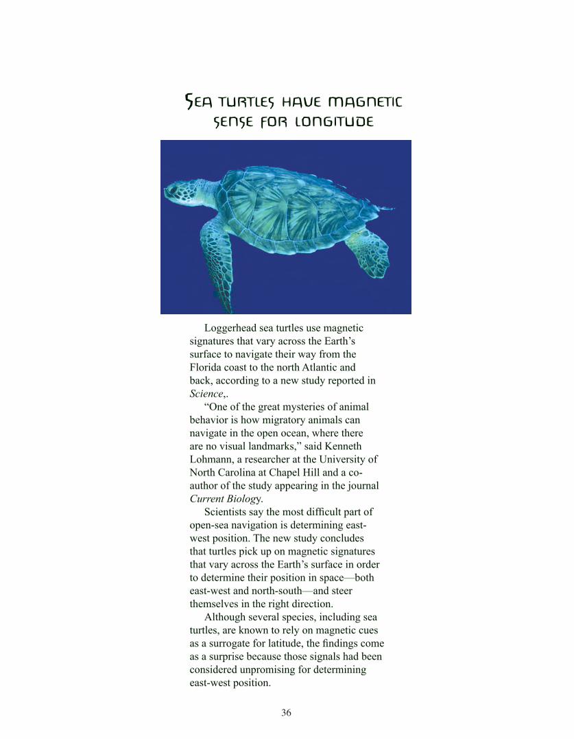
36

Sea turtleS have magnetic SenSe for longitude

Loggerhead sea turtles use magnetic signatures that vary across the Earth’s surface to navigate their way from the Florida coast to the north Atlantic and back, according to a new study reported in Science,.

“One of the great mysteries of animal behavior is how migratory animals can navigate in the open ocean, where there are no visual landmarks,” said Kenneth Lohmann, a researcher at the University of North Carolina at Chapel Hill and a co-author of the study appearing in the journal Current Biology.

Scientists say the most difficult part of open-sea navigation is determining east-west position. The new study concludes that turtles pick up on magnetic signatures that vary across the Earth’s surface in order to determine their position in space—both east-west and north-south—and steer themselves in the right direction.

Although several species, including sea turtles, are known to rely on magnetic cues as a surrogate for latitude, the findings come as a surprise because those signals had been considered unpromising for determining east-west position.

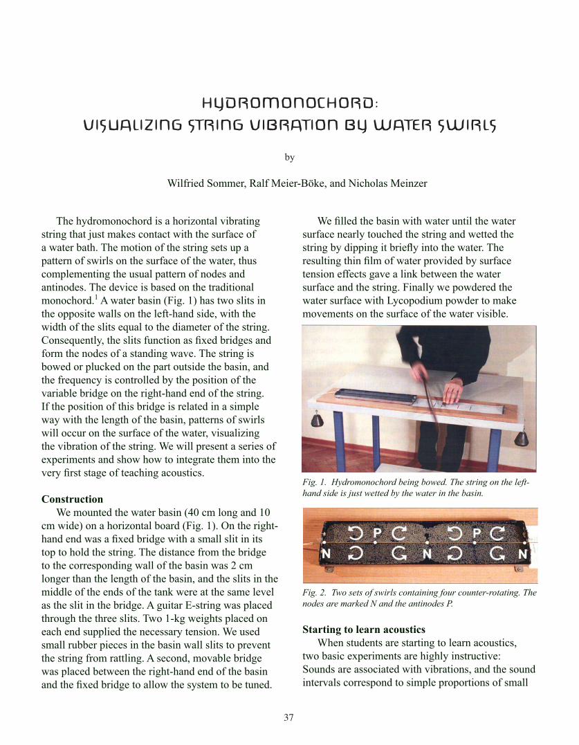
37

The hydromonochord is a horizontal vibrating string that just makes contact with the surface of a water bath. The motion of the string sets up a pattern of swirls on the surface of the water, thus complementing the usual pattern of nodes and antinodes. The device is based on the traditional monochord.1 A water basin (Fig. 1) has two slits in the opposite walls on the left-hand side, with the width of the slits equal to the diameter of the string. Consequently, the slits function as fixed bridges and form the nodes of a standing wave. The string is bowed or plucked on the part outside the basin, and the frequency is controlled by the position of the variable bridge on the right-hand end of the string. If the position of this bridge is related in a simple way with the length of the basin, patterns of swirls will occur on the surface of the water, visualizing the vibration of the string. We will present a series of experiments and show how to integrate them into the very first stage of teaching acoustics.

Construction We mounted the water basin (40 cm long and 10

cm wide) on a horizontal board (Fig. 1). On the right-hand end was a fixed bridge with a small slit in its top to hold the string. The distance from the bridge to the corresponding wall of the basin was 2 cm longer than the length of the basin, and the slits in the middle of the ends of the tank were at the same level as the slit in the bridge. A guitar E-string was placed through the three slits. Two 1-kg weights placed on each end supplied the necessary tension. We used small rubber pieces in the basin wall slits to prevent the string from rattling. A second, movable bridge was placed between the right-hand end of the basin and the fixed bridge to allow the system to be tuned.

HYDROMONOCHORD:VISUALIZING STRING VIBRATION BY WATER SWIRLS

by

Wilfried Sommer, Ralf Meier-Böke, and Nicholas Meinzer

We filled the basin with water until the water surface nearly touched the string and wetted the string by dipping it briefly into the water. The resulting thin film of water provided by surface tension effects gave a link between the water surface and the string. Finally we powdered the water surface with Lycopodium powder to make movements on the surface of the water visible.

Fig. 1. Hydromonochord being bowed. The string on the left-hand side is just wetted by the water in the basin.

Fig. 2. Two sets of swirls containing four counter-rotating. The nodes are marked N and the antinodes P.

Starting to learn acoustics When students are starting to learn acoustics,

two basic experiments are highly instructive: Sounds are associated with vibrations, and the sound intervals correspond to simple proportions of small

38

of the swirls is—compared to other methods-a very simple vibration detector. 3,4

Since the part of the string vibrating in air is a little bit longer than the length of the basin, the students can move the variable bridge slowly from one side to the other while plucking or bowing the string and reach several resonant positions. While doing this the forefinger of one hand holds the string firm on the variable bridge while the other hand bows or plucks. At the resonant position the swirls form very quickly, while in between only irregular movements are observed.

If one changes the tension of the string by pressing down the string with one finger directly after the bridge, the students can hear the increasing pitch of the plucked string while the pattern of the water swirls does not change. The crucial point is the wavelength of the standing wave in the string, which depends on the position of the variable bridge.

Second experiment: to raise octaves When the students compare the situation when the

variable bridge is set so that it is half the length of the basin from the right-hand end of the basin, and then the one in which it is a quarter of the distance (while keeping the tension constant), they find that the pitch of the plucked or bowed string goes up one octave. Simultaneously the flowing pattern in the water basin changes from two sets of swirls to four sets.

The comparison of the 2/3-position to the 1/3-position of the variable bridge, which involves a jump of an octave as well, is a little bit more complicated since the water pattern does not change. It is up to the teacher to decide if harmonics are to be mentioned to this level of students. They can certainly see that the set of swirls that occurs at the 2/3-position belongs to the first harmonic.

Further experimental challenges As an experimental challenge on a more advanced

level, one can try to go from two or four sets of swirls over the length of the water basin up to seven sets. From our experience it will be necessary to bow and not to pluck the string to accomplish this, and the variable bridge is put to the 1/5-, 1/6- or 1/7 -position in order to develop the corresponding number of sets. It is essential that the water has completely stopped moving when the bowing of the string starts.

numbers (traditional monochord experiments). The highly symmetric Chladni patterns, produced by bowing the edges of thin circular or rectangular plates that have had fine sand spread on their upper surfaces, can give students a feel for the numerical and geometrical order being involved in the phenomena of sounds.2 The Chladni patterns will occur when the vibrating sand migrates to the lines of nodes as the plate vibrates. The hydromonochord connects both of these ideas: the simple proportions of the intervals originating from the length of the bowed or plucked string on the one hand and the pattern of the vibrating string visualized by water swirls on the other hand.

We developed the hydromonochord for our introductory physics course so that students can see these two impressive phenomena coming together in one experiment. In this way they are able to realize the marvelous order as a signature of physics, especially, as the perceptions of several senses contribute to this experimental result. The following experiments focus on this signature for learning and understanding physics. We do not intend a systematic approach to standing wave phenomena or harmonics at this level.

First experiment: the occurrence of swirls In this first experiment the formation of swirls

is demonstrated. If the variable bridge is adjusted so that the distance from it to the right-hand end of the basin is a small number fraction of the length of the basin (especially 1/4,1/3,1/2, or 2/3), a set of swirls will occur as soon as the string is bowed or plucked.

At resonance, the surface of the water always contains sets of four counter-rotating swirls. In Fig. 2 the nodes are indicated by N and the antinodes by P. In each swirl the motion of the water next to the string and at the edge of the basin is parallel to the string, and at the nodes and antinodes the water moves perpendicular to the string. Students are able to connect the vibration of the string and the set of corresponding swirls by following two arguments: The antinodes of the string function as drivers for the formation of swirls. The nodes are relatively calm, since the outward flowing water of the swirls continues its rotation, reaching the walls of the basin, turning back, and starting to move along the string once more. In this sense the setting

39

If the variable bridge is almost touching the fixed bridge, the bowed length of the string will be equal to the length of the water basin. At this position we expected only one set of swirls to occur by bowing the string. We succeeded sometimes in the production of only one set, but in most cases we got the second or third harmonic, which means two or three sets of swirls.

These experimental exercises emphasize the connections of vibration and sound. Simultaneously students look upon the close connection of fundamental oscillations and their harmonics.

Acknowledgment The authors wish to thank Klaus Charisius,

retired, for his significant early work on the hydromonochord.

References 1. Ben Saferstein, “Resurrecting the Pythagorean

monochord,” Phys. Teach. 29,438–439 (Oct. 1991).

2. T. D. Rossing and N. H. Fletcher, Principles of Vibration and Sound, 2nd ed. (Springer, New York, 2004), p. 71.

3. Donald E. Hall, “Sacrificing a cheap guitar in the name of science,” Phys. Teach. 27, 673–677 (Dec. 1989).

4. E. Brock Dale, “Classroom demonstration of the vibration of a bowed string,” Am. Phys. 44, 1077–1079 (Nov. 1976).

AuthorsWilfried Sommer is assistant professor for

school pedagogy focusing on phenomenological teaching methods, a physics teacher at the Waldorf School Kassel, teacher trainer at the Kassel Teacher Training College, and a member of the board of directors of the Pedagogical Research Centre of the Federation of Waldorf Schools. Alanus University for Arts and Social Sciences, Faculty of Education, Villestr. 3, 0-53347 Alfter, Germany; wilfried.sommer@alanus.edu.

Ralf Meier-Bäke is an engineer with the Pedagogical Research Centre of the Federation of Waldorf Schools, responsible for the production of experimental equipment, and member of the team for the development of the hydromonochord. Padagogische Forschungsstelle Kassel, Brabanter Str. 30, 0-34131 Kassel, Germany; lehrmittel@lehrerseminar-forschung.de.

Nicholas Meinzer, a student, during an internship, was concerned with development of the hydromonochord. Pädagogische Forschungsstelle Kassel, Brabanter Str. 30, 0-34131 Kassel, Germany; nick@meinzer.info

40

And while I stood there I saw more than I can tell and I understood more than I saw; for I was seeing in a sacred manner the shapes of all things in the spirit, and the shape of all shapes as they must live together like one being. And I saw that the sacred hoop of my people was one of many hoops that made one circle, wide as sunlight and as starlight, and in the center grew one mighty flowering tree to shelter the children of one mother and one father. And I saw that it was holy. – Black Elk

Around Christmas the buds set and the bushes radiate a blood-like hue. Even though the earth’s crust is cold and solid, the mystery of growth ensues, dark-ly, quietly, and steadily. Traditional cultures around the world have danced, sung, and prayed at the winter solstice to hasten the sun’s return.

Early Egyptian myths imply that the sun was within a lioness, Sekhmet, at night and could be seen reflected in the eyes of the cow. Ancient Celts built raised stone, sun-round earthly circles where they worshiped and prayed for the Sun Goddess to return and the priests did astronomical sightings to gauge when the first seeds could be planted. Early Scandina-vian peoples sacrificed female animals to feed the Sun Goddess and hasten her journey back higher into the sky. During the later periods of Roman history, sun worship gained in importance and ultimately led to what has been called a “solar monotheism.” Nearly all the gods of the period were possessed of solar quali-ties. The feast of Sol Invictus (Unconquered Sun) on December 25 was celebrated with immense joy, and eventually this date was taken over by the Christians

RETURN OF THE SUN AFTER THE DARKEST DAYS

as Christmas, the celebrated birthday of Christ. The seventh-century Japanese held boisterous celebra-tions to entice forth the Sun Goddess from her seclu-sion in a cave.

The Native American tribes who practiced sun dance were:

• Arapaho• Arikara • Asbinboine • Cheyenne • Crow • Gros • Ventre • Hidutsa • Sioux • Plains Cree • Plains Ojibway • Sarasi

41

• Omaha • Ponca • Ute • Shoshone • Kiowa• Blackfoot

Their rituals varied from tribe to tribe. In North Amer-ica, many Native American tribes such as the Kiowas and Sioux , for example, had cults of ritualistic sun dancers. The Dakota Indians called the Sun “the mysterious one of day” and believed that this deity watched over them in time of need.

We Are One With The Infinite Sun Forever And Ever And Ever. – Native American

Some of these same cultures used stone observatories to track the annual path of the sun, and all were adept at reading natural signs that pointed to the turning of the seasons. So most winter solstice ceremonies probably served as celebrations of an expected but nonetheless reassuring event.

Signs of approaching spring can appear long before the year’s shortest day. On sun-warmed shales in the foothills of the Rockies, early Easter daisies (Townsendia exscapa and T. hookerii) begin blooming right around Thanksgiving. Nearby, both pasture sage (Artemisia ludoviciana) and fringed sage (A. jrigida) sprout aromatic green leaves.

Along the rivers, creeks, and streams, great horned owls begin courting in October, hooting deep into the night as they re-establish nesting territories. Some fe-males will lay their eggs by mid-January. Most bald eagle pairs have reconstructed their rough nests made of twigs and tree branches by the time the winter solstice arrives.

At the ponds, common goldeneyes cruise across the water in devoted pairs, while wood duck males fight and splash over mates. Groups of courting wigeons fly over-head in tight diamond formation like an Air Force flight demonstration team at the county fair.

By a quirk of astronomy—stemming from the inter-action of the tilting Earth with its elliptical orbit around the sun—where I live in Colorado the earliest sunset falls around Dec. 9, nearly two weeks before the shortest day. As total daylight keeps diminishing, the afternoons gradually grow longer, hinting at the rising of the sun in the heavens and renewal of vegitation that it promises.

As we celebrate the sun’s return, we find the occa-sional warmth-filled rays of the sun massaging our faces as the days lengthen. Our spirits lift with this unantici-pated grace and its promise of renewed spring growth. We look toward the heavens and observe bald eagles and flocks of Canada geese fly over the frosted grasslands along the lower river beds. As the wisemen of the Narive Americans chanted:

To pray you open your whole selfTo sky, to earth, to sun, to moon,To one whole voice that is you.And know there is moreThat you can’t see, can’t hear,Can’t know except in momentsSteadily growing, and in languagesThat aren’t always sound but otherCircles of motion.Like eagle that Sunday morningOver Salt River. Circled in blue skyIn wind, swept our hearts cleanWith sacred wings.We see you, see ourselves and knowThat we must take the utmost careAnd kindness in all things.Breathe in, knowing we are made ofAll this, and breathe, knowingWe are truly blessed because weWere born, and die soon within aTrue circle of motion,Like eagle rounding out the morningInside us.We pray that it will be doneIn beauty. – Native American

– DSM

42

Experiment

A Mini RobotIngredients:

• an old sonic toothbrush with angled bristles

• a pager motor (www. goldmine-elec.com)

• solder

• black electrical tape

• thin insulated copper wire

Procedure:

• Cut off the head of the toothbrush using a small back-saw

• Solder two wires to motor.

• Stick the motor and battery to the tape and watch the brush hop about.

43

There are many ways that soap can be made. Here is one example.

Ingedients:

• 2 oz. of olive oil • 3 pounds of Crisco shortening or organic vegetable shortening • 12 oz. of water (Distilled water is best.) • 6 oz. lye (sodium hydroxide, micro beads) • food coloring (optional, red or yellow will work adequately) • essential oil (lavender, honeysuckle, hibiscus or other from your local herb shop)

Equipment:

• glass bowl • wooden spoon • safety glasses • mold

Procedure: • Melt and heat the Crisco in a water bath stirring with a wooden spoon • Place cold water in a glass bowl and slowly add and mix in the lye while stirring with a wooden

spoon. Stir until water is clear if you can. (Caution, use safety glasses and ensure that lye doesn’t get in eyes!)

• After the Crisco has completely melted, mix in the lye and then the olive oil. • When the Crisco and lye are warm to the touch, pour lye into Crisco while stirring. Keep

stirring until you get trace.

Trace is when it thickens to the point where you can drop some of the mix back in to itself and it leaves a trail.

• Add scent (choice from a local herb shop) and color (food coloring) if desired and pour into mold(s). This recipe fits nicely in an 8 x 8 inch container.

• Put molds in a warm, insulated place, let set 24 hours and then cut. Place on a rack and let cure for 2–3 weeks in the open air at room temperature.

Experiment

Making Soap

44

Building anElectric Motor

(see Science Kit #12)

45

46

47

Teaching Sensible Science Course

Began in February, 2011

The fourth round of Teaching Sensible Science Course began at the Chicago Waldorf School with the largest enrollment to date. This is an excellent training course for class teachers who want to prepare themselves for teaching the science curriculum in Grades 6 through 8.

The course is comprised of three, one-week sessions, each focusing on the Physics and Chemistry curricula of a specific grade. Led by Michael D’Aleo, participants enrich their understanding of the philosophical underpinnings of the phenomenological approach to teaching science and benefit from lots of practical advice and experience in presenting the demonstrations and experiments. This course is highly recommended.

For more information or to register for the next series, contact the director of the program, Michael D’Aleo, at: spalight@verizon.net.

48

Index of Past Issues

Waldorf Science Newsletteredited by David Mitchell © AWSNA Publications

This newsletter is published once a year and is dedicated to developing science teaching in the Waldorf schools. Teachers are in vited to pose questions, seek resource material, discuss experiments, write about their classes (suc-cessful and not very successful), and investigate phe nomena. The editor also translates relevant science articles from Waldorf periodicals from around the world. The following past editions are available from:

AWSNA PublicationsE-mail: publications@awsna.org

458 Harold Meyers RoadEarlton, NY 12058 fax: 518/ 634-2597

phone: 518/ 634-2222

available on-line at: http://www.whywaldorfworks.org/books_sciencenews.htm

Volume 1, #1 Partial contents – Acoustics in Grade 6; Teaching about Alcohol in Grade 8 Chemistry; The Chemistry Curriculum: The Debate over Teacher Demonstration vs. Student Experimentation; Spiritual Aspects of 20th Century Science; Overview of the Waldorf Science Curriculum; Water; Characteristics of the Major Sugars; Goethe’s Meditation on Granite; Book Reviews; Humor; Poetry; Conferences; and Sample Experiments Volume 1, #2 Partial contents – The Characteristics of Drugs; Eratosthenes Revived; The Golden Number; Educational Guidelines for a Chemical Formula Language; The Properties of Acids and Bases; Walter Lebendörfer on Chemistry; Biology in the 11th Grade; What Is Home?; The Waldorf Environmental Curriculum; Environmental Education; Women in Science; Book Reviews; Humor; Poetry; Conferences; and Sample Experiments

Volume 2, #3 Partial contents – Grade 12 Physics – Von Mackensen; Biology Teaching in the 11th Grade; Euclid’s Algorithm; The Logos and Goethean Observation; Nature Education; Aristotle’s Taste Spectrum; Book Reviews; Humor; Poetry; Conferences; and Sample Experiments

Volume 2, #4 Partial contents – Current Research; Strange Theories; Science Education and Wonder; The Human Earth; Steiner’s Counterspace Examined; The Cow; Language and the Book of Nature; Book Reviews; Humor; Poetry; Conferences; and Sample Experiment

Volume 3, #5 Partial contents – Book Reviews; First Lessons in Astronomy; Steps in the Development of Thinking (Power of Judgment); Computer Science and Computers in the Waldorf School; Technology; Computers in Education; Some Characteristics of the Computer; Computers and Consciousness; Experiments

Volume 3, #6 Partial contents – Space and Counter Space; New Eyes for Plants; Experiments of Academia dell Cement; Physics and Chemistry in the Grades; Goethean Science Credits; Chemistry Workshop; Table of Important Salts; Goethe’s Scientific Imagination; To Infinity and Back in Class 11; π and Trigonometry; Science in the Waldorf Kindergarten; A Note on Pascal’s Triangle; Experiments

Volume 4, #7 Partial contents – The Message of the Sphinx; Honey; Cell Cosmology; Einstein’s Question; What Is Goethean Science?; Prototype Computer Program; River Watch as a Classroom Activity; Thoughts on Curriculum Standards; Comments on Building a Waldorf School; Experiments

49

Volume 4, #8 Partial contents – Towards Holistic Biology; How DNA Computers Work; Solar System Facts; What Is Goethean Science?; Human Movement and the Nervous System; What Is Science?; What Is Meant by “Teaching the Children to Breathe?”; Experiments

Volume 5, #9 Partial contents – The Globe Inside Our Planet; Music, Blood and Hemoglobin; Standards in Science; Cognitive Channels—the Learning Cycles and Middle School Students; 8th Grade Physics, From Dividing to Extracting Roots; What Is Lambda?; Waldorf Science Kits

Volume 5, #10 Partial contents – Reading the Rocks; Why the Arts Are Important to Science; The Three Groups of Rocks; Introduction to Geology; The Rock Cycle; Mineralogy for Grade 6; Metals and Minerals, Precious Stones—Their Meaning for Earth, the Human Being, and the Cosmos; Experiments

Volume 6, #11 Partial contents – A Chemistry of Process; Sponges and Sinks and Rags; How to Read Science; Experiences and Suggestions for Chemistry Teaching; Experimentation as an Art; Biographies—Dmitri Mendeleev, Joseph Priestley, Marie Curie; Destructive Distillation; Experiments

Volume 6, #12 Partial contents – Light and Darkness in 6th Grade Physics; The Relation of “Optical Elevation” to Binocular Vision; Description of Curves in Connection with Elevation Phenomena; Water Treatment at the Toronto Waldorf School; A Lime Kiln that Can Be Assembled and Disassembled; Experiments

Volume 7, #13 Partial contents – Thoughts on Returning to an “Education Towards Freedom”; Pedagogical Motives for the Third Seven-Year Period; Social Education through Mathematics Lessons; A Vision for Waldorf Education; Our Approach to Math Doesn’t Add Up; International Mathematics Curriculum

Volume 7, #14 Partial contents – Conferences; Physiology, Update on Taste; Pictorial Earthquake; Boiling with Snow; Towards a Waldorf High School Science Curriculum for the 21st Century; The Thermal Decomposition of Calcium Carbonate; Crystals Reveal Unexpected Beginnings; Cosmic Ray Studies on Skis; Experiments

Volume 8, #15 Partial contents – Book Reviews; Arabic Science; Arabic Mathematics: Forgotten Brilliance; Making Natural Dyes; Exploring the Qualities of Iron; Von Mackensen Chemistry Conference; Oalic and Formic Acid; Hydraulic Rams; What the Water Spider Taught Me

Volume 8, #16 Partial contents – Waldorf High School Research Papers; Inside the Gulf of Maine; How Do Atomistic Models Act on the Understanding of Nature in the Young Person?; The House of Arithmetic; Origami Mathematics; Sixth Grade Acoustics; Sixth Grade Kaleidoscopes; Tricks with Mirrors; The Flour Mill and the Industrial Revolution; Web Gems; Understanding Parabolic Reflectors; The Capacitor; Oscillation and Waves; Crystal Radio; Qualifications for High School Mathematics Teaching

Volume 9, #17 Partial contents – Book Reviews; Acknowledgement from a Waldorf Parent; Raising Money for Science; The Twelve-Year-Old Child and Orpheus; Towards a Sensible Kind of Chemistry, Part One; The Lightning Bug; The Ladybug; Exploratory Experimentation: Goethe, Land, and Faraday; Faraday’s Synthetic Investigation of Solenoids; Faraday’s Analytic Investigation of Induction; Geometric Addition Table: A Curious Configuration

Volume 9, #18 Partial contents – Book Reviews; Towards a Sensible Kind of Chemistry, Part Two; The Evolution of the Fast Brain; Professors Vie with Web for Class Attention; The Teenage Edge; Oscillator Coil Demonstration Using an Ultra-Low Frequency LC-“Tank” Circuit; Thermodynamic Experiments for the Middle School

50

Volume 10, #19 Partial contents – Book Reviews; The Beaver; Nature in the Human Being; Astronomy Verses for the Middle School; Child Development and the Teaching of Science; Bibliography for Middle School Teachers; What Is Phenomenology?; The Design of Human and Animal Bodies; The Brain and Finger Dexterity; Observations of a Neurophysiologist

Volume 10, #20 Partial contents – Book Reviews; A Number Story for the Sixth Grade; Novel Entries for a Trig Table; An Introduction to the Sine and Tangent; Toss Out the Toss-Up: Bias in Heads or Tails; Phlogistron Theory; Song of the Rain; Refrigeration in Physics; The Poetry of Astronomy; Build Your Own Sextant; Highlights from Recent Science-teaching Periodicals; Websites of Interest

Volume 11, #21 Partial contents – Books of Interest; A Sampling of Poems for Botany; How Does Sense-Nerve System Activity Relate to Conscious Experience?; Acoustics in Sixth Grade; Fun Facts of Physiology; About Formative Forces in Vertebrates and Human Beings; Global Perspective; Points to Consider in Science Teaching; Deconstructing

Black Box; Aspects of a Computerized Physics Lab

Volume 12, #22 Partial contents – Books of Interest; Preserving a Snowflake; Environment, Morphology, and Physical Principles for Waldorf High School Teachers and Students, Part 1; Homemade Audio Speaker for Grade Eight; Mathematics and Natural Science: A Reflection from the Viewpoint of Pedagogy and the History of Ideas; Animal Sight; Kepler’s Model of the Universe; Teaching Sensible Science; Mug on a Glass: An Optics Demonstration for Grade Seven; Chemistry Challenge for Grade Eight; On Being an Insect; Surveying and Mapping: An Attempt to Integrate New and Emerging Technologies into the Class 10 Curriculum

Volume 13, #23 Partial contents – Books of Interest; Advice on Teaching 8th Grade Meteorology; An Explanation of the Phenomenological Approach for Parents of Middle School Children; Astronomy (Hubble Space Telescope Photographs); Environment, Morphology, and Physical Principles for Waldorf High School Teachers and Students, Part 2; Sensible Science Workshop; How Parachute Spiders Invade a New Territory; Pluto Is No Longer a Planet; Computer Curricula in U.S. Waldorf Schools; Experiments

Volume 14, #24 Partial contents – Books of Interest; Robotics; A Seventh Grade Fresco Project; A Pinhole Camera Project for the Seventh Grade; Other Projects for Elementary Physics Classes; The Aurora Borealis; Phenomenological Science Equipment; The Karma of Calculus—Involving Isaac Newton and Gottfried Leibniz; Award-Winning Photos of Nature and Animals; Humor

Volume 15, #25 Partial contents – Books of Interest; Doing Phenomenology in Science; The Western Screech Owl; Sea Turtles Use Earth’s Magnetic Field to Navigate; The World’s Biggest Bug; Tree Talk; The Phenomenology of Colored Shadows; Analemma; Photos from Hubble; Mechanics in 7th Grade Physics

Volume 16, #26 Partial contents – Books of Interest; Going through, Taking in, Considering: A Three-Phase Process of Learning as a Method of “Teaching in Main Lesson Blocks”; The Geometry of Life: Toward a Science of Form; Phenomenology: Husserl’s Philosophy and Goethe’s Approach to Science; First Approach to Mineralogy; Growing Salt Crystals; The Beauty of Slime Molds; An Interview with Daniel Pink; Mutualism between Elk and Magpies; Symbiotic Relationships

Volume 17, #27 Partial contents – Books of Interest; Points to Consider in Teaching Science; A Brief Overview of the Waldorf High School Mathematics Curriculum; Some Fun Facts of Physiology; The Imaginary in Geometry; Volcanism; Hydromonochord: Visualizing String Vibrations by Water Swirls; Return of the Sun after the Darkest Days; Experiments