Embed Size (px)
Citation preview

The Psychometric Properties of the GSS Wordsum Vocabulary Test
Neil Malhotra (corresponding author) Department of Political Science
Stanford University Encina Hall West, Room 100
Stanford, CA 94305 Phone: 408-772-7969
Email: [email protected]
Jon A. Krosnick Departments of Communication, Political Science, and Psychology
Stanford University 434 McClatchy Hall
450 Serra Mall Stanford, CA 94305 Phone: 650-725-3031 Fax: 650-725-2472
Email: [email protected]
Edward Haertel School of Education Stanford University
485 Lasuen Mall Stanford, CA 94305-3096
Phone: (650) 725 1251 Email: [email protected]
August, 2007
Jon Krosnick is University Fellow with Resources for the Future. This research was supported by a small grant from the Board of Overseers of the General Social Survey. We thank Yi Chun Chen for valuable research assistance.
The Psychometric Properties of the GSS Wordsum Vocabulary Test
Abstract
Social scientists in many disciplines have used the General Social Survey’s ten-item
Wordsum vocabulary test to study the causes and consequences of vocabulary knowledge and
related constructs. In adding up the number of correct answers to yield a test score, researchers
have implicitly assumed that the ten items all reflect a single, underlying construct and that each
item deserves equal weight when generating the total score. In this paper, we report evidence
suggesting that extracting the unique variance associated with each word and measuring the
latent construct only with the variance shared among all indicators strengthens the validity of the
index. We also report evidence suggesting that Wordsum could be improved by adding words of
moderate difficulty to accompany the existing questions that are either quite easy or quite
difficult. Previous studies that used Wordsum should be revisited in light of these findings,
because their results might change when a more optimal analytic method is used.
1
The Psychometric Properties of the GSS Wordsum Vocabulary Test
Cognitive abilities have received a substantial amount of attention from social scientists,
who have devoted a great deal of effort to building tools for measuring these skills, to be used
when testing theories of their causes and consequences. A frequently studied component of
intelligence is verbal skill: the ability to use, manipulate, and reason with language. Verbal
ability can be decomposed into fluid intelligence (which is the ability to manipulate information)
and crystallized intelligence (which is the cache of information acquired through experience and
stored statically in long-term memory; Cattell 1963, 1987; Horn and Cattell 1967). Our focus in
this paper is on an aspect of verbal crystallized intelligence: vocabulary knowledge (i.e., the
possession of word meanings).
Many tests have been constructed to measure vocabulary knowledge, most of them
lengthy and cumbersome. Well-known, long tests used in educational and psychological
research include the vocabulary items of the I.E.R. Intelligence Scale CAVD, the vocabulary
subtest of the Wechsler Adult Intelligence Scale-Revised (WAIS-R) (Wechsler 1981), the Mill-
Hill Vocabulary Scale (Raven 1982), the vocabulary section of the Nelson-Denny Reading Test
(Nelson and Denny 1960), the vocabulary subtest of the Shipley Institute of Living Scale
(Shipley 1946), and others. Some tests (e.g. the items from the I.E.R. Intelligence Scale CAVD)
are multiple-choice, whereas others (e.g. WAIS-R) ask respondents to provide open-ended
answers. The WAIS-R includes 35 vocabulary items in a 60 to 90-minute test; the Mill-Hill
scale is composed of 66 questions, constituting 25 minutes of testing time; the Nelson-Denny test
asks 80 vocabulary items in a 45-minute test; and the Shipley test includes 40 items in a 20-
minute assessment.
In contrast to these lengthy measures, the General Social Survey (GSS) has included a

2
much shorter ten-item, multiple-choice measure of vocabulary knowledge (called “Wordsum”)
in sixteen surveys of representative national samples of American adults since 1974. Wordsum
has been used to assess verbal skills (and even general intelligence sometimes) by scholars in a
wide array of disciplines, including sociology, political science, and psychology. Yet despite its
widespread use, the basic psychometrics of Wordsum have almost never been evaluated (though
see Bowles et al. 2005). All substantive research using Wordsum that we have uncovered has
assumed that the test captures a single, underlying factor, so the total number of correct answers
has been computed for use in analysis. In this paper, we explore the psychometric properties of
Wordsum to see whether there are better ways to analyze the resulting data and to see whether
the measure itself can be improved.
We begin by describing the history and format of Wordsum. Then, we review previous
studies that have used Wordsum, to document its ubiquity across the social sciences and to
underscore the importance of exploring its psychometric properties. The third section presents a
theoretical analysis of the measurement issues involved. Then, we present the results of two
studies of the psychometric properties of Wordsum, describing our data and findings and
discussing their implications.
The Test
In the early 1920s, Edward L. Thorndike developed a lengthy vocabulary test as part of
the I.E.R. Intelligence Scale CAVD to measure, in his words, “verbal intelligence.” As in the
modern-day Wordsum test, each question asked respondents to identify the word or phrase in a
set of five whose meaning was closest to a target word. Robert L. Thorndike (1942) later
extracted two subsets of the original test, each containing twenty items of varying difficulty. For
each subset, two target words were selected at each of ten difficulty levels. The ten items in

3
Wordsum (labeled with letters A though J) were selected from the first of these two subsets.
Prior to its initial use in the 1974 GSS, a slightly different version of Wordsum was used in
another national survey: National Opinion Research Center (NORC) Study SRS-889A (1966).
However, neither Thorndike nor NORC recorded why they selected the particular set of items to
be included in that survey. Without understanding how the items were chosen, we cannot know
whether the designers of the test intended to measure a single dimension or multiple dimensions
of verbal intelligence.
The Wordsum measure has been administered using a show card that interviewers have
handed to GSS respondents during interviews in their homes. Each item of the test is multiple-
choice, consisting of a prompt word in capital letters and five responses choices (as well as a
“don’t know” option), all numbered and in lower-case. Some response choices are single words,
while others are phrases.1 The instructions provided to respondents are:
“We would like to know something about how people go about guessing words
they do not know. On this card are listed some words—you may know some of
them, and you may not know quite a few of them.
On each line the first word is in capital letters—like BEAST. Then there are five
other words. Tell me the number of the word that comes closest to the meaning
of the word in capital letters. For example, if the word in capital letters is BEAST, you
would say ‘4’ since ‘animal’ comes closer to BEAST than any of the other words.
If you wish, I will read the words to you. These words are difficult for almost
everyone—just give me your best guess if you are not sure of the answer. CIRCLE ONE
CODE NUMBER FOR EACH ITEM BELOW.
1 The administrators of the GSS keep the list of prompt words and responses choices confidential to avoid contamination of future surveys, so we cannot describe them here.

4
EXAMPLE
BEAST 1. afraid 2. words 3. large 4. animal 5. separate 6. DON’T KNOW”
The Ubiquity of Wordsum in the Social Sciences
Analyzing the psychometric properties of Wordsum is important, because scores on the
test have been used extensively as both an independent variable and a dependent variable in
much previous research. A literature search of social science journals, books, and edited
volumes published between 1977 and 2000 uncovered 38 studies that used Wordsum. Table 1
presents the distribution of publications by scholarly field. The majority of studies have been
published in sociology, political science, education, and psychology, though Wordsum has
appeared in publications of other disciplines as well. In this section, we review a portion of these
studies to illustrate Wordsum’s utility in the social sciences.
Constructs Measured Using Wordsum
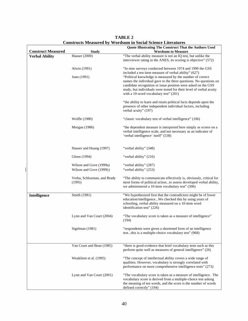
Scholars have used Wordsum to measure many constructs, listed in Table 2 according to
frequency of use. Nine studies used Wordsum to measure verbal ability; eight used it to measure
the broader construct of general intelligence. Interestingly, fewer studies (seven) used Wordsum
to operationalize exactly what it is, a test of vocabulary. And some scholars have used the test to
measure concepts such as cognitive sophistication, knowledge of standard English words,
linguistic complexity, and receptivity to knowledge.
Findings of Research with Wordsum
Many scholars have examined hypothesized determinants and consequences of
vocabulary knowledge as measured by Wordsum using GSS cross-sectional data. Although
methodological techniques exist for causal inference using the sort of cross-sectional,
observational data that the GSS has entailed (e.g. covariance structure modeling, instrumental
5
variables regression, propensity score matching), the vast majority of the evidence, which we
review next, is correlational.
Several scholars have used Wordsum to explore the effect of vocabulary knowledge on
socioeconomic and life success, testing the controversial hypothesis that society has become
increasingly stratified by ability (Herrnstein and Murray 1994). Walberg and Weinstein (1984)
documented a positive relation between vocabulary scores and socioeconomic status (SES), and
Hauser and Huang (1997) found that this relation did not change between 1974 and 1994.
Weakliem, McQuillan, and Schauer (1995) observed that class differences in Wordsum scores
were smaller in cohorts born after 1945 than in cohorts born earlier, challenging the hypothesis
that vocabulary knowledge and occupational status have become increasingly intertwined.
Other scholars have explored the relation between vocabulary knowledge and educational
attainment. Many observers believe that the American education system, through reading and
writing tasks, improves students’ abilities to comprehend language and to use it effectively.
Hyman, Wright, and Reed (1975) did find that more educated people had better vocabulary
knowledge. Wolfle (1980) discovered that most of the impact of education is indirect and occurs
via adult intelligence. Smith (1993) showed that the education gap in Wordsum scores is greater
for earlier birth cohorts, suggesting that the relation between education and vocabulary
knowledge has diminished over time. Blake (1989) found that at each level of educational
attainment, vocabulary knowledge scores were negatively related to the number of siblings a
respondent had. This supports the confluence model (Zajonc and Markus 1975), which asserts
that a child’s intellectual development is dependent on the average level of intelligence in his or
her household, which decreases as more children are added. Finally, Loeb and Bound (1996)
suggested that school characteristics such as lower student-teacher ratios and longer term lengths

6
significantly increase Wordsum scores.
Other correlates of vocabulary knowledge have also been studied using Wordsum. For
example, Morgan (1986) found that people who spent more time watching television scored
lower on Wordsum. Lewis (1990) reported that public bureaucrats had higher Wordsum scores
than did the general public, while Glenn and Hill (1977) found that urban and suburban
respondents did better on Wordsum than did rural respondents. Nash (1991) observed that
African-Americans scored lower on Wordsum than whites, even when controlling for SES.
A small, yet controversial research literature has emerged regarding the presence of
cohort differences in Wordsum scores. Alwin (1991) and Glenn (1994) attributed the drop in the
mean Wordsum score over time to lower scores among cohorts born after World War II. Wilson
and Gove (1999a, 1999b) critiqued these studies by claiming that the decline in scores over time
is an artifact of adjusting cohort test scores for differences in education. As a result, the across-
time pattern of Wordsum scores may be due to aging, providing support for the cognitive aging
hypothesis (Schaie 1996), which states that vocabulary ability (a form of “crystallized”
intelligence) increases until the mid-fifties. Alwin and McCammon (1999) repeated Alwin’s
analysis but controlled for aging and again found that decreases in Wordsum scores over time
were best explained by cohort differences. Glenn (1999) found between-cohort differences in
vocabulary knowledge scores but not within-cohort differences in scores according to age,
refuting Wilson and Grove’s aging hypothesis.
Other studies have used Wordsum to measure cognitive skills and intelligence more
broadly. Miner (1957) found that scores on Wordsum and more elaborate IQ tests were strongly
correlated (r=.8 or higher), suggesting that verbal skills are a good measure of general cognitive
ability. Bobo and Licari (1989), Arthur and Case (1994), and Case, Greeley, and Fuchs (1989)
7
used Wordsum as a measure of cognitive sophistication, which they found to be significantly and
negatively related to political intolerance, support for police force, and racial prejudice,
respectively. These findings were viewed as consistent with the hypothesis that intelligence
increases tolerance. Sigelman (1981) used Wordsum to represent general intelligence and
reported evidence that less intelligent people are no happier than the general population, refuting
the folk wisdom that “ignorance is bliss.” Van Court and Bean (1985) and Lynn and Van Court
(2004) examined the relation between Wordsum scores and fertility, concluding that less
intelligent people (as measured by vocabulary knowledge) are more fertile. Rempel (1997) used
Wordsum as a proxy for cognitive mobilization (e.g. the possession and use of advanced
intellectual capacities), which he argued causes people to develop a unidimensional liberal-
conservative political ideology. Finally, Hauser (2000) used vocabulary scores as a proxy for
cognitive ability, which he found to predict voter turnout.
Wordsum has also been used by survey methodologists analyzing how respondents
answer questions. Krosnick and Alwin (1987) demonstrated that respondents with lower
Wordsum scores were most prone to response order effects in surveys. These investigators
concluded that response order effects occur because respondents with limited cognitive skills are
most likely to shortcut the cognitive processes entailed by generating optimal answers to
questions. Smith (1981) found that respondents with lower Wordsum scores were more likely to
provide logically contradictory answers to different questions. Smith (1992) also discovered that
respondents with higher Wordsum scores were more likely to provide substantive answers to
sexual behavior questions instead of giving “don’t know” responses.
Some studies of political participation have used Wordsum to measure constructs other
than vocabulary knowledge and general intelligence. For example, Junn (1991) treated

8
Wordsum as an indicator of political knowledge, which she found to increase participatory
activity. Verba, Schlozman, and Brady (1995) found that people with higher Wordsum scores,
which the authors used to represent civic skill and the ability to politically communicate, were
more likely to participate in the political process.
In conclusion, numerous studies conducted over the past thirty years have uncovered a
host of variables that seem to correlate with Wordsum in ways that have advanced theory-
building in the social sciences. The ubiquity of Wordsum suggests that a closer examination of
the measure is warranted.
Theoretical Overview of Measurement Approaches
The studies described above all operationalized vocabulary knowledge by summing the
number of correct responses on the test and then including that number in statistical models.
Hereafter, we refer to this approach as the “additive technique.” To justify such an
operationalization, one must assume not only that the items tap a single underlying dimension of
vocabulary knowledge but also that each item deserves equal weight when gauging that
dimension through addition. In other words, the unique variance associated with each word is
equal and random, not systematic. However, if some items better capture the construct of
vocabulary knowledge, then this assumption may be untenable.
Other approaches to measurement would permit researchers to relax this assumption and,
consequently, may more validly represent vocabulary knowledge. For instance, item response
theory (IRT; Baker 2004) presumes that a latent construct can be tapped by dichotomous test
items and that the probability of a correct response to an item is a function of the respondent’s
level of the construct. Item parameters characterize the form of this function for each specific
item. In widely used “two-parameter” models, items are assumed to differ according to two

9
parameters: difficulty and discrimination. Item difficulty is inversely related to the probability of
providing a correct response; harder items are answered correctly by fewer respondents. The
discrimination parameter measures an item’s ability to distinguish between respondents on the
high and low ends of the latent construct. Items that poorly discriminate are unable to bifurcate
respondents into groups with different values on the latent scale. Hence, not all items are
“created equal,” since some are more effective than others at identifying respondents’ locations
on the latent scale. Consequently, the simple additive technique of combining a set of items may
not be optimal; poorly discriminating items may dilute the validity of the summed score.
IRT posits that a set of test items ideal for measuring with uniform accuracy over a broad
range of ability would possess two characteristics: (1) they should be highly discriminating,
meaning that they should be able to distinguish the ability levels of respondents; and (2) they
should have a broad range of levels of difficulty. Hence, researchers should select the most
discriminating items at each of various difficulty levels to construct an index. In this way, the
total scores on the test can effectively stratify respondents by ability levels. Individuals
possessing low values of the latent construct will usually not receive high scores, and those at
high values of the construct will usually not score poorly.
Another school of thought is the latent variable approach, which would treat vocabulary
knowledge as a latent construct that is the cause of responses to a set of observed variables, such
as responses to test items (Skrondal and Rabe-Hesketh 2004). Unlike the summation technique,
latent variable modeling does not assume that the unique variance in each item is random and
equal. Rather, this approach separates the unique variance in each item from the shared variance
common to all the items. The shared variance would be presumed to constitute the construct of
vocabulary knowledge.

10
The IRT and latent variable approaches can be implemented presuming that responses to
all the test items place respondents on a single latent continuum. And given what research has
documented about vocabulary development, this may be a sensible assumption. The theory of
crystallized intelligence claims that vocabulary knowledge is developed during a distinct stage
early in life and then maintained (Horn and Cattell 1967). Furthermore, this base of knowledge
is reinforced throughout life through use of words in everyday activity. New vocabulary is then
added to this foundation (Cattell 1987). However, crystallized intelligence theory also posits that
vocabulary accumulation during adulthood is specialized and esoteric, implying that vocabulary
knowledge may be comprised of multiple dimensions (Cattell 1998). Moreover, the dual
representation theory of knowledge suggests that vocabulary knowledge is characterized by
multiple representations differing in their level of specificity (Brainerd and Reyna 1992). Some
aspects of verbal ability deal with general meanings of words, whereas others are responsible for
more specific definitions, implying that vocabulary skill may not be best represented by a unitary
factor.
Previous studies examining the dimensionality of vocabulary knowledge have employed
factor analysis to assess its underlying structure. Bailey and Federman (1979) and Beck et al.
(1989) identified two underlying factors of the WAIS-R intelligence items but interpreted them
differently. The former study concluded that the WAIS-R test measured breadth and depth
dimensions, whereas the latter identified a standard vocabulary factor and an advanced
vocabulary factor. In the only factor-analytic examination of the GSS’s Wordsum test, Bowles
et al. (2005) also identified two dimensions: basic vocabulary and advanced vocabulary. They
reported loadings on these factors that corresponded closely to the item difficulties, with one
factor largely defined by the four easy items and the other by the six difficult items. The
11
possibility that these were merely artifactual “difficulty” factors was thoughtfully addressed and
ruled out to the extent possible using alternative methods of nonlinear factor analysis and
correction for guessing.
In order to test the superiority of a two-factor structure over a one-factor structure, it is
useful to explore whether the two factors are differently associated with other variables. Bowles
et al. (2005) showed this to be so for age, cohort, and education, which were significantly
differently related to the two vocabulary knowledge factors.
Study One: A Psychometric Analysis of Wordsum
Overview of Analyses
Our goal in this paper is twofold: (1) to reassess the dimensionality of Wordsum by a
different method: analyzing how individual words behave in correlational analyses, to see
whether their factor structure might be more complex than prior research suggested; and (2) to
compare two analytic approaches to measuring the latent construct(s) of interest: the approach
used most often in past research (simply adding up the number of correct responses) vs. latent
variable covariance structure modeling. If the latent structure of Wordsum is in fact more
complex than just two factors and yet researchers want to measure a single principal factor, then
using covariance structure modeling can extract the unique variance in each item and
operationally define vocabulary knowledge as the variance common to all items, yielding more
precise measurement and perhaps different substantive findings.
We evaluate the unidimensionality hypothesis by testing six hypotheses. The first three
treat vocabulary knowledge as a dependent variable, and the latter three treat it as a predictor.
Vocabulary Knowledge as the Dependent Variable
Hypothesis 1: If the ten items all reflect a single underlying construct, then they should
12
correlate similarly with predictors of vocabulary knowledge.
For each of the ten words, we predicted whether a respondent correctly answered an item
with variables expected to correlate with vocabulary knowledge, such as the year in which the
survey was conducted (Alwin 1991), age (Wilson and Gove 1999a, 199b), education (Hyman,
Wright, and Reed 1975), parental education, and media consumption (Morgan 1986). If
Wordsum is unidimensional, then the relations between these variables and the probability of
answering an item correctly should be similar across words. However, if the individual items
and the criterion measures correlate idiosyncratically, then the underlying factor structure is
likely to be more complex.
Hypothesis 2: If the ten items all reflect a single underlying construct, then using
arbitrary subsets of the Wordsum items rather then the full set of items to measure vocabulary
knowledge should produce weaker associations but no substantive shifts in the results of
correlational analyses.
We randomly selected words from Wordsum to create two four-item subscales. We then
predicted these scale scores with the same correlates mentioned above. Unidimensionality
would be confirmed if we obtained consistent estimates regardless of which subset is used,
whereas observing heterogeneous results across the subscales would attest to the
multidimensionality of the Wordsum items.
Hypothesis 3: If the ten items all reflect a single underlying construct and adding up the
number answered correctly effectively removes measurement error, then using the latent
variable approach to extract the unique variance in each test item should produce comparable
parameter estimates and variance explained in models predicting vocabulary knowledge as does
the simple additive technique.

13
We estimated the parameters of latent variable covariance structure models predicting
vocabulary knowledge with the variables mentioned above. In one set of models, vocabulary
knowledge was measured perfectly by the summed score using all Wordsum items or one of two
four-item subscales. In another set of models, vocabulary knowledge was a latent variable that
determined responses to individual items. This method extracts the unique variance in each test
item in order to construct a composite latent construct measure tapping only the variance shared
among all indicators. We assessed whether this approach yielded stronger relations between
vocabulary knowledge and its correlates and more variance explained.
Vocabulary Knowledge as the Independent Variable
Hypothesis 4: If the ten items all reflect a single underlying construct, then they should
perform similarly in analyses using vocabulary knowledge as a predictor.
We used the ten individual items as independent variables when estimating the
parameters of regression equations predicting voter turnout and political tolerance, two popular
dependent variables that past research has posited are consequences of vocabulary knowledge as
measured by Wordsum. We replicated regressions from Hauser’s (2000) study of the
determinants of turnout and Bobo and Licari’s (1989) analysis of the predictors of political
tolerance. If Wordsum is unidimensional, then the ten words should correlate similarly with
turnout and tolerance. However, if the individual items predict the two variables
idiosyncratically, that would suggest that a more complex psychometric structure exists.
Hypothesis 5: If the ten items all reflect a single underlying construct, then using
arbitrary subsets of the Wordsum items rather then the full set of items to predict turnout and
tolerance should produce weaker but substantively comparable results in correlational analyses.
Using the two four-item subscales from the test of Hypothesis 2, we used vocabulary
14
knowledge to predict voter turnout and political tolerance using the Hauser (2000) and Bobo and
Licari (1989) regression equation specifications. Unidimensionality would be confirmed if we
obtain consistent but weaker estimates, regardless of which subset is used, whereas observing
heterogeneous results across the subscales would attest to multidimensionality of the Wordsum
items.
Hypothesis 6: If the ten items all reflect a single underlying construct, then using the
latent variable approach to extract the unique variance of each test item should produce the
same parameter estimates and variance explained in models predicting tolerance and turnout as
does the simple additive technique.
We computed the parameters of covariance structure models predicting turnout and
tolerance with vocabulary knowledge, measured in two ways. In one set of models, we
measured vocabulary knowledge with a summed score using all Wordsum items or using the two
four-item subscales described above. In another set of models, we treated vocabulary knowledge
as a latent variable that was posited to cause responses to the individual items. If we observe
stronger relations of vocabulary knowledge with its correlates and more variance explained when
using the latent variable approach than when using the additive approach, that would suggest that
Wordsum taps multiple constructs. In other words, extracting the unique variance of the words
would strengthen the associations between vocabulary knowledge and its correlates.
In all the analyses we conducted, political tolerance was also represented as a latent
variable measured by the fifteen dichotomous items in the GSS civil liberties battery. Voter
turnout was simply an observed, dichotomous variable. Mplus was used, so we could relax the
assumption of continuity by estimating covariance structure models with limited dependent
variables as probability models, which assume that continuous latent variables underlie

15
categorical outcomes (as in logistic regression).
Data
The GSS is a series of national surveys that have been conducted twenty-six times by the
National Opinion Research Center (NORC) since 1972. Interviews were conducted face to face
with a representative, national area probability cluster sample of the English-speaking American
adult population not living in institutions (e.g., college dorms, nursing homes). We focused on
the administrations of Wordsum in fifteen surveys conducted between 1974 and 2000. The
sample size per survey was about 1,500 between 1974 and 1990 and has approached 3,000 since
1994. Response rates have ranged from 70% to 80% (National Opinion Research Center 2004).
In some years, the test was administered to only a random subset of the respondents rather than
to all of them. Of the 43,698 people interviewed in these fifteen surveys, the total number of
respondents who took the test in its entirety is 19,879. Appendix 1 explains technical issues
involving weighting, clustering, and handling of missing data.
Results
Wordsum is composed of two groups of words: six “easy” words and four “hard” words
(see Figures 1 and 2). A majority of respondents (65.7%-95.3%) correctly answered items D, B,
A, F, I, and E, whereas a minority of respondents (19.2%-35.7%) accurately identified words G,
H, J, and C. Interestingly, no words were moderately difficult, being answered correctly by
about half of the sample.
To conduct an IRT analysis to assess each item’s difficulty and level of discrimination,
we used BILOG-MG (Zimowski, Muraki, Mislevy, & Bock, 1996) and estimated the parameters
of a three-parameter model to control for respondent guessing (see Appendix 2 for details). This
uncovered great heterogeneity in the items’ abilities to discriminate between respondents high

16
and low in vocabulary knowledge. Among the “easy words,” word F discriminates well,
whereas words A and I are uninformative in stratifying individuals according to vocabulary
knowledge (see Table 3). Similarly, among the “hard” words, word H appears to discriminate
better than word C. These findings indicate that the Wordsum items have unique properties,
suggesting that they may not all represent a common, underlying dimension. Therefore, a more
careful examination of each individual item seems warranted. Furthermore, these results suggest
that the test may be improved through the addition of moderately difficult words, a possibility we
will explore later.
Vocabulary Knowledge as the Dependent Variable
Hypothesis 1
First, we assessed whether the relations of correct responses to each of the ten items with
year, age, education, parental education, and media consumption were consistent across words.2
Wordsum responses were coded 1 if the word was correctly identified and 0 if not or if the
respondent said he or she did not know the answer. Parameter estimates from logistic
regressions predicting correct responses for each word are presented in the first ten columns of
Table 4.
Heterogeneity among items with respect to the temporal changes in correct responses is
quite apparent, suggesting that Wordsum may be representing multiple factors (see row 1 of
Table 4). Time was coded to range from 0 to 1, with 0 representing the earliest year (1974) and
1 representing the latest year (2000). For some words (D, A, E), the probability of observing a
correct response was unrelated with time. For the remainder (B, F, I, G, H, J, C), a negative
relation is observed: fewer correct answers in later years. Introducing a quadratic term to permit
2 These variables were chosen because they allowed us to pool together as many waves of the GSS as possible while including an array of predictors in regression equations.

17
a nonlinear relation did not produce consistency across words. Among the seven words for
which there was a negative relation, the quadratic term was positive and significant for three (F,
I, H), positive and insignificant for two (B, J), and negative and insignificant for two (G, C).
Among the three words for which there was no linear relation, for only one word (A) does
including a quadratic term produce a negative, significant linear effect and a positive, significant
quadratic effect. This suggests that different words may be tapping different constructs, as
evidenced by differences between them in terms of trends over time.
The relation between correct response and age also varied across words, again pointing to
a multifactorial psychometric structure (see rows 2 and 3 of Table 4). Age was coded to range
from 0 to 1, with 0 representing the youngest person across all surveys and 1 representing the
oldest person. For most words, a nonlinear relation appeared: middle-aged respondents
answered the items correctly more often than did the young and the elderly. However, for two
words (D and F), the quadratic term was statistically insignificant, implying a monotonic
increase in vocabulary knowledge with age. The probability of providing a correct response to
word J, on the other hand, appears to have been completely unrelated to age.
The effect of education on vocabulary knowledge was concave for easy words and
convex for hard words. Education was coded using four dummy variables representing five
different levels. Respondents with less than a high school education were treated as the baseline
category. To illustrate the meanings of the parameters, the predicted probabilities of observing a
correct response (holding all other variables at their means) are plotted against level of education
in Figures 3 and 4. For easy words, being a high school graduate greatly increased the
probability of providing a correct response, but little was gained from additional education.
Conversely, for hard words, the probability of providing a correct response only increased

18
substantially among people with a bachelor’s degree or more education. Thus, easy items
require only a little bit of schooling, whereas hard items necessitate post-secondary education.
With respect to parental education, the results were much less consistent, with different
degree levels achieving statistical significance for different words. These results again suggest
that the assumption of a single factor of vocabulary knowledge may not be appropriate.
We next examined the relations between Wordsum items and media consumption.
Newspaper readership was coded to range from 0 (meaning the respondent never read a
newspaper) to 1 (meaning read a newspaper seven days a week) and television viewing was
coded to range from 0 (meaning the respondent never watched television) to 1 (meaning watched
television twenty-four hours a day). For every word, more newspaper reading was associated
with increased vocabulary knowledge, although the strengths of the coefficients varied across
words. Conversely, watching more television generally decreased performance on the Wordsum
items, though Words A and I did not manifest this relation. Thus, these correlational analyses
suggest that the ten items may not be consistently tapping a single construct of vocabulary
knowledge or even two factors.
Hypothesis 2
Next, we predicted scores on two four-item subscales: one built using Words A, C, H, I,
and the other built using Words D, E, F, G. Both sets constituted mixtures of “hard” and “easy”
words. To ensure direct comparability, all scales were coded to range from 0 (answering none of
the items correctly) to 1 (answering all items correctly). Coefficients from regressions predicting
the number of correct responses on the entire Wordsum scale as well as the two four-item
subscales (labeled “Four-Item A” and “Four-Item B”) are presented in the final three columns of
Table 4.

19
The coefficients were generally larger when predicting the “Four-Item B” scale than
when predicting the “Four-Item A” scale, suggesting that the former may be a more valid
measure of vocabulary knowledge. Of the seventeen variables used to predict vocabulary
knowledge, six were significantly larger for the “Four-Item B” scale, at the 90% significance
level. If Wordsum taps a single dimension of vocabulary knowledge, then the relations of a set
of covariates with subscales of the test should not vary depending on the particular words
included in the subscale. Although this seems to have been so if one glances quickly at the
coefficients, closer examination suggests systematic differences.
Hypothesis 3
Next, we estimated the parameters of covariance structure models predicting vocabulary
knowledge with the full set of predictors. In one set of models, vocabulary knowledge was
treated as measured perfectly by a single indicator: the total number of correct Wordsum
responses (using either all ten items or the two four-item subsets). In a second set of models,
vocabulary knowledge was measured by multiple indicators (the individual test items), each with
error. These two approaches differ in two ways: (1) the latter extracts the unique variance of
each item from the total score, whereas the former includes that unique variance, and (2) the
latter approach does not impose the constraint that all items be weighted equally, whereas the
former approach does.
To compare the effectiveness of the two analytic approaches, we estimated the
parameters using Mplus and compared the goodness of fit of various models.3 In all of these
models, the predictors (e.g. age, education, etc.) were treated as being perfectly measured by
3 Because responses to the individual items are dichotomous, the measurement model equations representing the effect of latent vocabulary knowledge on each item’s score were estimated within a logistic regression framework.
20
single indicators. The path diagrams can be found in Appendix 3.
The multiple indicator models fit better than the models constructed using the simple
additive approach (see Table 5). The R2 of the model using the 10-item total score was .26,
dramatically lower than that for the model in which the ten items were separate multiple
indicators (R2 = .46). Similar results were produced with the four-item subscales. Interestingly,
the fits of the models using the multiple indicator approach with the “Four-Item A” and “Four-
Item B” (R2 = .36 and .41, respectively) subsets are superior to the model fit obtained when using
the single-indicator 10-item score (R2 = .26). These findings suggest that relaxing the
assumption of equal item weights and extracting unique item variance when measuring
vocabulary knowledge produces much better explanatory results.
Vocabulary Knowledge as the Independent Variable
Hypothesis 4
Next, we estimated the parameters of covariance structure models using vocabulary
knowledge to predict political tolerance and voter turnout, replicating Hauser’s (2000) and Bobo
and Licari’s (1989) regressions. Political tolerance was measured with a fifteen-item battery
constructed with questions asking about respondents’ support of three civil rights (to make a
speech, teach in a college, and author a book kept in a public library) of five social groups
(atheists, communists, racists, fascists, and homosexuals). For each group, respondents were
asked whether members should be allowed to make the speech, whether members should be
“fired” from the college, and whether the book should be removed from the library. All items
were dichotomous, and the civil liberties score was the sum of tolerant responses. Turnout was
measured by a question asking whether the respondent voted in the most recent presidential
election. We included in our regressions the same demographic and political control variables

21
included by the authors in their original work.4
Again, we found that the individual words behaved differently from one another, pointing
to multidimensionality. Replicating Hauser’s (2000) regression predicting turnout with the ten-
item score, we found the same strong positive relation (b = 2.73, p<.001, see column 1 of Table
6). When we relaxed the assumption of equal weight by including all the individual items as
separate predictors, we observed large between-item heterogeneity in coefficient size, regardless
of whether all items were predictors in a single equation or each item was the sole predictor, one
at a time (see columns 2 and 3). According to chi-square tests evaluating differences between
coefficients, item E was the strongest predictor; its coefficient was significantly larger than those
of all other items except Word F. One item (I) had an associated coefficient that was
significantly weaker than all the rest and in fact had a non-significant partial association with
turnout when controlling for all the others. Since both of these words are “easy,” item difficulty
does not anticipate which questions will predict turnout. All items were statistically significant
predictors of turnout when they were included as the only measure of vocabulary knowledge in
the equation, but the coefficients varied considerably in size, ranging from .49 to .96 (see column
3).
We obtained similar findings when replicating Bobo and Licari’s (1989) work predicting
political tolerance (see Table 7). The ten-item index was a strong predictor of tolerance (see
column 1), but only four items (E, G, I, J) were significant predictors of tolerance, whereas the
other six were not (see column 2). Again, item difficulty was unrelated to predictive
effectiveness, since E and I are “easy” words and G and J are “hard.” When including each
4 Information on the coding of covariates can be found in the original articles. Despite considerable effort, we were unable to replicate their regression results exactly, although our estimates were extremely close. Most importantly, our estimates involving vocabulary knowledge were statistically indistinguishable from the estimates reported by the authors.

22
vocabulary test item as the sole predictor, Item B still manifested no significant association, and
the other words had significant associations but of notably varying strength, rangin from .54 to
1.57 (see column 3). All of these findings challenge the assumption of equal item weighting.
Hypothesis 5
The “Four-Item B” scale’s coefficient was larger than the “Four-Item A” scale’s when
predicting both outcomes (see Tables 6 and 7). This difference was significant with regard to
turnout (Δb = .33, p=.004), though not with regard to tolerance (Δb = .34, p=.63). Again, this
suggests that Wordsum does not tap a single dimension of vocabulary knowledge, since the
relations between tolerance/turnout and the score varied depending on the particular words
included in the subscale.
Hypothesis 6
Finally, we explored the value of extracting the unique variance of each of the items by
constructing covariance structure models predicting tolerance and turnout with vocabulary
knowledge. Vocabulary knowledge was represented both as a measured variable using the
additive technique and as a latent variable that caused answers about each individual word.
Political tolerance was represented as a latent variable that caused its fifteen indicators. Turnout
was represented as a perfectly measured construct: respondents’ reports of whether or not they
voted in the previous presidential election (the loading was fixed at one, and the error variance
was constrained to be zero). We performed this exercise using all ten Wordsum items and using
the two four-item subscales.
The results suggested that past analyses may have considerably underestimated the
strengths of the relations between vocabulary knowledge and its covariates by using the simple
additive Wordsum score. Parameter estimates generated using Mplus for the turnout analysis are

23
presented in the left-hand side of Table 8. Isolating the variance common to all ten words
produced a nearly 50% improvement in model fit compared to summing correct responses (see
Table 8). Furthermore, using only four words from the “Four-Item B” scale to predict
vocabulary knowledge did even better than using all ten (R2=.19). However, variance explained
when using the “Four-Item A” scale was slightly lower. This is consistent with the finding that
the “Four-Item A” subscale was a much weaker predictor of turnout than the “Four-Item B”
scale (see Table 3).
Similar results appeared when predicting political tolerance with vocabulary knowledge
(see right-hand side of Table 8). The variance explained in the dependent variables was more
than one-and-a-half times as large when extracting the unique variance of each of the ten items
than when simply adding up the number of correct answers. Similar patterns appeared when
using the two four-point subscales. In fact, treating vocabulary knowledge as a latent construct
and using the four words from the “Four-Item A” scale produced nearly as strong as an
association as using all ten words. Additionally, the variance explained varied depending on
which subset of words was used, again suggesting a complex psychometric structure of
Wordsum. Thus, in using Wordsum, relaxing the assumption of unidimensionality and freeing
the weights on the individual items appears to have improved measurement considerably.
Study Two: Potential Improvements to Wordsum
Overview
Because Wordsum currently includes items of very high difficulty (fewer than one-third
of Americans answer these correctly) or very low difficulty (more than three quarters of
Americans answer these correctly), IRT suggests that it can be improved by adding moderately
difficult words with a percent correct between 40% and 60%. This would allow the test to

24
discriminate better among people whose vocabulary knowledge is in the middle range. In fact,
test design experts urge that it is especially important to have items of moderate difficulty in such
a test (e.g., Minnema et al. 2000), yet Wordsum has none.
We therefore explored the possibility of adding additional items to the existing Wordsum
battery. A natural place to look for items to add is the vocabulary section of the I.E.R.
Intelligence Scale CAVD, since Wordsum is itself a subset of this larger test. Although we have
been unable to locate any CAVD test results from the last few decades, we developed a
technique to determine which of the CAVD test words were most likely to be moderately
difficult using the frequency of the words’ occurrence in popular news media stories.
Our approach was based on the assumption that the more frequently a word is used in
news stories, the more people are likely to know its meaning. Such an association between word
frequency in news stories and public understanding of the words could result from two
phenomena: (1) the news media might avoid using words that people do not understand; and/or
(2) people might be more likely to learn the meanings of words to which they are exposed more
frequently in news stories. Either way, frequency of appearance in news stories might serve as
an indicator of item difficulty.
To test this hypothesis, we began by using Lexis-Nexis to count the number of stories in
The New York Times that contained each of the ten Wordsum words in the headline or lead
paragraph between 1982 and 2000, the years for which data are available. With those data, we
estimated the parameters of the following regression equation:
Percent Correcti = βLn Storiesi + εi.
where Percent Correcti is the percent of respondents who correctly answered the Wordsum
question about word i, and Storiesi is the number of news stories that included word i in the

25
headline or lead paragraph.
A standardized estimate of the relation between the natural log of the number of stories
and the percent correct was .68 (R2 = .46, p=.03), a very strong relation. The unstandardized
coefficient is 13.04, meaning that a 1% increase in the number of stories was associated with a
.13 percentage-point increase in correct responses. This suggests that we could use the
frequency of news media mentions of words in the CAVD that are not in Wordsum to predict the
percent of Americans who would define each word correctly.
To begin the process of selecting candidate items for adding to Wordsum, we randomly
selected thirteen words from the intermediate levels of the CAVD (which are the levels from
which the Wordsum items were selected - Levels V3, V4, V5, V6, and V7).5 We then generated
predicted percent correct scores for these words using their frequency in news stories. Seven of
the words had predicted percent correct scores between 40% correct and 60% correct: “New
Word 2” (41.0% correct), “New Word 1” (41.6% correct), “New Word 16” (43.5% correct),
“New Word 9” (43.6% correct), “New Word 18” (48.7% correct), “New Word 14” (52.9%
correct), and “New Word 5” (53.8% correct). These therefore seemed worthy of further
investigation.
We used a second source of information to identify potential words to add as well: the
results of tests administered by Thorndike (1927) to high school seniors on various occasions
between 1922 and 1925, as described in his book The Measurement of Intelligence. Clearly, this
respondent pool is very different from a national probability sample of American adults living
today. However, the correlation between percent correct for the ten Wordsum words in the
1922-1925 Thorndike sample and the 1974-2002 GSS samples is a remarkable .83, meaning that
5 Because these items may eventually be included in Wordsum, we do not describe them here and refer to them anonymously (e.g. “New Word 1,” “New Word 2,” etc.).

26
the difficulty rankings and the differences in difficulties between words was consistent across
datasets. Hence, the Thorndike results may be a reasonable proxy with which to select items for
testing with the American public today.
In Thorndike’s data, 17 words were correctly defined by between 42% and 62% of high
school seniors: “New Word 20” (42.0%), “New Word 15” (42.0%), “New Word 19” (43.1%),
“New Word 21” (43.5%), “New Word 22” (45.1%), “New Word 6” (45.7%), “New Word 23”
(46.2%), “New Word 3” (49.5%), “New Word 4” (49.8%), “New Word 13” (51.0%), “New
Word 9” (52.5%), “New Word 10” (55.9%), “New Word 7” (58.4%), “New Word 8” (60.5%),
“New Word 11” (61.0%), “New Word 12” (61.6%), and “New Word 17” (61.6%). One of these
words (“New Word 9”) was also identified by our method using news story frequency to guess
item difficulty, making it an especially appealing candidate. Using all the items for which we
had both predicted percent correct from our news story frequency analysis and also from
Thorndike’s testing, the correlation between the predicted percent correct was r=.40.6 Thus,
there was some correspondence between the two methods for this set of words, though
correspondence was far from perfect.
To gauge whether these methods identified test items that would in fact be moderately
difficult and therefore useful additions to Wordsum, we administered 23 items from the CAVD
(the seven words from the news story analysis and the seventeen words from the Thorndike
administration, one of which overlapped with the words from the news story analysis) to a
general population sample of American adults to ascertain the percent of people who answered
each one correctly. The Thorndike items each offered five response options (the correct answer
plus four distracters) in addition to the target vocabulary word. We also administered the ten
Wordsum items to assess comparability of results from this sample to those obtained in the GSS. 6 Three words were not administered by Thorndike (1927).

27
Data
The 23 new test items were included in an Internet survey of 1,498 volunteer American
adult respondents conducted by Lightspeed Research in January, 2007. Lightspeed's panel of
potential survey respondents is recruited in three principal ways: (1) people who register online
for something at a website and agree to receive offers from other organizations are later sent
emails inviting them to join the Lightspeed panel to complete survey questionnaires, (2) people
who register online for something at a website and check a box at that time indicating their
interest in joining the Lightspeed panel are later sent emails inviting them to complete the
Lightspeed registration process, and (3) banner advertisements on websites invite people to click
and join Lightspeed's panel. Using results from the U.S. Census Bureau’s Current Population
Survey, Lightspeed Research quota sampled its panel members in numbers such that the final
respondent pool would be reflective of the U.S. population as a whole in terms of characteristics
such as age, gender, and region. Post-stratification weights were constructed so that the sample
matched the U.S. population in terms of education, race, age, and gender.
Results
The proportion of the Lightspeed respondents answering the ten Wordsum questions
correctly was higher than the proportion of GSS respondents doing so, by an average of 7.6
percentage points (see the top of Table 9). Nonetheless, the ranking of difficulties of the ten
Wordsum items was about the same in both surveys. In fact, the correlation between the percent
correct across the ten items was a staggeringly high r=.99. Hence, results from the Lightspeed
survey for the 23 proposed new words (shown at the bottom of Table 9) may be quite
informative about how GSS respondents would answer the items.
To anticipate the percent correct for these words likely to occur in a general public

28
sample, we estimated the parameters of an OLS regression predicting GSS percent correct with
Lightspeed percent correct using the ten Wordsum words. The coefficient estimates for the
intercept and slope were -6.9 (p=.16) and .99 (p<.001), respectively. Hence, on average, there
was a nearly perfect 1:1 relationship between GSS and Lightspeed percent correct, save for the
6.9 percentage point intercept shift. Correcting for this discrepancy, we calculated predicted
values from the regression, thereby estimating how the new words would perform in a
probability sample of the general population (see the second column in the bottom panel of Table
9).
According to this method, twelve words (bolded) manifested predicted percents correct in
the moderate range: New Words 7-18. If even a few of these words were appended to the current
Wordsum battery, the test would likely become more discriminating and better able to tap the
latent variable of vocabulary knowledge.
To select the most desirable candidates among these words, we sought to identify those
with the highest discrimination parameters from an IRT analysis. Our first step in this process
involved conducting IRT analyses with data on the ten Wordsum items in the Lightspeed
Research dataset. The estimated discrimination and difficulty parameters are reported in the last
two columns in the top panel of Table 9. The correlations between the discrimination and
difficulty parameters across the GSS and Lightspeed data were r=.82 and r=.97, respectively.
This, too, inspires some confidence in use of the Lightspeed data for identifying new items.
Using all 33 words in the Lightspeed dataset (the 10 Wordsum items and the 23 possible
additions), we again estimated a three-parameter IRT model, producing discrimination and
difficulty statistics for the proposed additional words (see the last two columns in the bottom
panel of Table 9). Words with the highest discrimination scores are the most appealing to add to

29
Wordsum⎯the four highest were “New Word 8,” “New Word 9,” “New Word 12,” and “New
Word 16” (in the shaded rows of Table 9).
Finally, we conducted a series of analyses to explore the impact of adding these four
words to Wordsum, either in addition to the current ten words or replacing the four least
desirable words according to IRT methods. We examined the performance of a longer, fourteen
item scale because, in practical application, the GSS might retain the original ten items to
continue the time series and simply add supplemental words. However, we also examined a
revised ten-item measure replacing four current Wordsum items, because adding four items will
almost always improve scale performance. By holding the number of items constant, we
explored the advantages of incorporating moderately difficult items into Wordsum.
In constructing a test to measure ability along a latent scale (as opposed to constructing a
test to bifurcate individuals above and below a given cut point), IRT suggests selecting highly
discriminating items at equally spaced difficulty levels (Embretson and Reise, 2000). According
to these guidelines, we selected Words A and I for elimination, because of their low
discrimination power (see Table 3). We also removed Words B and C, because they had
redundant difficulties with Words D and J, respectively but had low discrimination parameters
(see Table 3). The resulting set of words was more equally spaced in terms of difficulties.
Using the Lightspeed Research data, these additions clearly altered the observed
distribution of vocabulary knowledge scores (computed by adding up the number correct). In the
new distributions, shown in the bottom of Figure 5, the numbers of respondents decline fairly
smoothly as the percent correct declines from right to left. One might imagine that the more
normal distribution, shown at the top of Figure 5 for the original Wordsum words for both the
GSS and Lightspeed data, would be more psychometrically desirable. But the Lightspeed data

30
suggest that the distributions shown in the bottom of Figure 5 may more accurately describe the
distribution of vocabulary knowledge in the American public.
As shown in Figure 6, revising Wordsum to include moderately difficult items makes the
test information curves conform more closely to the ideals of IRT. For the current ten items, the
test information curve has a valley at the middle of the ability dimension, reflecting the paucity
of moderately difficult items (see top of Figure 6). Replacing redundant and poorly
discriminating words with moderately difficult words produces a test high in information at all
ability levels.
To see whether changing the distribution by adding the four new words changed the
validity of the composite score, we conducted OLS regressions predicting vocabulary knowledge
scores using the two demographics available in the Lightspeed dataset that we had also used in
the regressions presented in Table 4: age and education.7 To generate a baseline for comparison,
we predicted total Wordsum score using the ten current items in the most recent GSS data (see
the first column on Table 10) and in the Lightspeed Research data (see column 2). We then
conducted the same regression after replacing words A, B, C, and I with the four new words of
moderate difficulty and yet again after adding the four new words to the full set of ten (see the
last two columns of Table 10).
The regression coefficients for the demographics were stronger and more statistically
significant when predicting the revised ten-item measure of vocabulary knowledge than when
predicting the original measure. Indeed, the percent of variance explained by the two
demographics increased by fully three percentage points. Interestingly, adding back the four
7 In the Lightspeed data, we found no quadratic effect of age on vocabulary knowledge when including a squared term for age. In the regression predicting the current tem items, the coefficients for age and age squared were b=-.10 (p=.60) and b=.29 (p=.13), respectively. In the regression predicting the revised Wordsum index, the coefficients for age and age squared are b=.16 (p=.53) and b=.10 (p=.71), respectively.

31
discarded words made the coefficient estimates weaker and did little to increase the variance
explained. Hence, adding moderately difficult items to Wordsum strengthened the relations
between vocabulary knowledge and theoretically sensible covariates, suggesting that the latent
construct of vocabulary knowledge can be better measured using a slightly different battery.
Similarly, when we estimated structural equation models using Mplus in the manner
described above (i.e. with the latent variable of vocabulary knowledge predicting responses to
the items individually), we again found that the introduction of moderately difficult items
enhanced the correlational validity of the battery. As shown in Table 11, the relations of age and
the education dummies with the latent vocabulary knowledge variable were stronger when using
the revised ten- and fourteen-item measures than when using the original ten items.
Furthermore, the measurement model fit the data better as well, suggesting that the moderately
difficult items do better at discriminating respondents near the center of the latent dimension of
vocabulary knowledge.
Finally, we explored how test scores from the revised battery including the four
moderately difficult items mapped onto scores from the original, ten-item test. Table 12 presents
a cross-tabulation of scores from both tests with cell percentages from the Lightspeed data. On
average, respondents’ scores on the additional Wordsum items were similar to their scores on the
original ten. Whereas respondents averaged 66.8 percent correct on the current Wordsum test,
they answered 68.1% correct on the four additional items (weighted).
Discussion
In this paper, we sought to explore the underlying dimensionality of Wordsum. Such a
close examination seemed warranted given the ubiquity of the measure across the social sciences
and the fact that all researchers implicitly assumed that the test tapped a single, underlying

32
construct of vocabulary knowledge. Each of our six sets of analyses pointed to a complex
psychometric structure, unable to be explained by one or two latent dimensions.
1. When treating vocabulary ability as the dependent variable, the relations between a set
of predictors (time, age, respondent and parental education, media consumption) and the
probability of a correct answer were not completely consistent across the ten individual items.
2. Wordsum manifested different relations with a set of predictors depending on whether
we used all ten Wordsum items or one of the two four-item subscales, a result inconsistent with
unidimensionality or bidimensionality.
3. Using a latent variable approach to discard the unique variance in each item and
measure vocabulary knowledge with the shared variance yielded more explanatory power
predicting vocabulary knowledge, political tolerance, and voter turnout as compared to the
simple additive technique.
4. Vocabulary knowledge predicted tolerance and turnout differently depending on which
of the ten individual items we used.
5. Tolerance and turnout were related to vocabulary knowledge differently depending on
which of the two four-item subscales was used.
These results all suggest that the ten Wordsum words have different relations with
various criteria because responses to the items manifest a considerable amount of unique,
systematic variance. If a researcher simply sums the number of correct responses to calculate a
total score out of ten (or sums a subset of the items), then the systematic unique variance of each
word is included in that score. The item-specific variances do indeed appear to be non-random,
meaning that estimates from statistical models that simply analyze a total Wordsum score will be
distorted by measurement error. So when researchers are interested in the shared variance

33
common to all indicators to represent general vocabulary knowledge, the latent variable
approach seems to be an effective way to isolate this shared variance and remove the distorting
influence of unique variance in particular items.
These findings suggest potential value in revisiting previous studies that used Wordsum
to document the causes and consequences of vocabulary knowledge. Indeed, our replications of
two existing studies demonstrated that the stringent (but unmet) assumptions of the additive
technique can affect the substantive conclusions a researcher would reach. Therefore, it may be
worthwhile to build covariance structure models treating vocabulary knowledge as a latent
variable measured by the GSS ten items and exploring: (1) the impact of vocabulary knowledge
on socioeconomic success; (2) the impact of education on vocabulary knowledge; and (3) age-
time-cohort patterns. Revisiting these substantive topics with a new understanding of the
psychometric properties of Wordsum may help us shed light on previously undiscovered
intricacies in the causal processes at work involving vocabulary knowledge.
Similarly, our results are instructive for future users of Wordsum, regardless of whether
vocabulary is a central construct in the analysis or simply a control variable. When estimating
relations between Wordsum performance and other variables of interest, covariance structure
modeling seems merited. This approach may yield more valid parameter estimates. By only
using the total score, scholars have been throwing away valuable information and running the
risk of reaching incorrect conclusions.
Indeed, our findings in this regard may be of value not only to users of Wordsum but also
to other scholars who study constructs that are measured using batteries of items assumed to
represent a single, underlying dimension. As with vocabulary knowledge, the optimal method of
operationalizing these constructs may not be a simple addition of its constituent items.

34
Our findings also point to a way to improve GSS’s Wordsum test, by adding items of
moderate difficulty. Such additions would probably improve the IRT parameters of the test and
also considerably alter substantive findings involving Wordsum in constructive ways.

35
Appendix 1: Methodological Issues
In this appendix, we explain issues involved in performing the statistical analyses
including weighting, clustering, and handling of missing data.
Weighting
Three probability weights (FORMWT, OVERSAMP, ADULTS) from the GSS dataset
were multiplied together to yield the weight variable that was used in our analyses. First, the
data were weighted by demographics using the variable FORMWT.8 Second, the data were
weighted to account for black oversamples (OVERSAMP) in 1982 and 1987. Finally, since the
unit of analysis in this study is the individual, the data were weighted to account for household
size. This weight was equal to the number of adults in the household (ADULTS).
Clustering
Because the GSS uses block quota sampling, we took into account that random samples
were clustered by primary sampling unit (PSU). Using Stata 9.0’s and MPlus’s survey
commands, the statistical analyses take into account clustering by PSU, which is represented by
the variable SAMPCODE.
Missing Data
Instances in which a respondent did not choose an answer to a Wordsum question can be
considered incorrect when a respondent says “I don’t know which answer is correct.” but should
probably be treated as missing data points if the respondent says “I prefer not to take this test.”
and fails to answer all the questions. Therefore, respondents who declined to answer all 10
answers are dropped from our analyses. We also discarded data from respondents who “broke
off” from the test midway through (which we operationalized by declining to answer the last four
questions of the test). When we repeated our analyses using other cutoffs instead (the last 1, 2, 3, 8 The demographic characteristics used to construct the weights are not reported in the GSS codebook.

36
or 5 questions), the results obtained were the same.

37
Appendix 2: Three-Parameter Item Response Model
The three-parameter item response theory model is defined as:
)(11)1()(
jjeggP jjj βθαθ −−+
−+=
where Pj(θ) is the probability that respondent with abilityθ answers item j answers correctly, αj
is the item discrimination parameter, βj is the item difficulty parameter, and gi is the probability
of a correct response to a multiple-choice item as a result of guessing. The BILOG-MG software
employed marginal maximum likelihood (MML) estimation to obtain parameter estimates for
each item by integrating the likelihood function over the ability distribution (Bock and Aitken
1981).

38
Appendix 3: Path Diagrams of Latent Variable Models Predicting Vocabulary Knowledge
Multiple Indicator Model (Vocabulary Knowledge Predicts Items Individually) Single Indicator Model (Vocabulary Knowledge Predicts Additive Scale)
Vocab.Knowledge
G
H
J
C
D
B
A
F
I
E
Time
Age
Educ.
Fath.Educ.
Moth.Educ.
TV
News
Time
Age
Educ.
Fath.Educ.
Moth.Educ.
TV
News
Vocab.Knowledge
Time
Age
Educ.
Fath.Educ.
Moth.Educ.
TV
News
Time
Age
Educ.
Fath.Educ.
Moth.Educ.
TV
News
WordsumScale

39
TABLE 1
Number of Studies Using Wordsum by Scholarly Field
Field Number of Studies Sociology 14 Political Science 8 Education 5 Psychology 3 General Social Science 2 Statistical Methodology 2 Natural Sciences 1 Philosophy 1 Gerontology 1 Communication 1 Total 38
40
TABLE 2
Constructs Measured by Wordsum in Social Science Literatures
Construct Measured Study Quote Illustrating The Construct That the Authors Used
Wordsum to Measure Verbal Ability Hauser (2000) “The verbal ability measure is not an IQ test, but unlike the
interviewer rating in the ANES, its scoring is objective” (572)
Alwin (1991) “In nine surveys conducted between 1974 and 1990 the GSS included a ten-item measure of verbal ability” (627)
Junn (1991) “Political knowledge is measured by the number of correct names the individual gave to the three questions. No questions on candidate recognition or issue position were asked on the GSS study, but individuals were tested for their level of verbal acuity with a 10-word vocabulary test” (201) “the ability to learn and retain political facts depends upon the presence of other independent individual factors, including verbal acuity” (197)
Wolfle (1980) “classic vocabulary test of verbal intelligence” (106)
Morgan (1986) “the dependent measure is interpreted here simply as scores on a verbal intelligence scale, and not necessary as an indicator of ‘verbal intelligence’ itself” (538)
Hauser and Huang (1997)
“verbal ability” (348)
Glenn (1994)
“verbal ability” (216)
Wilson and Gove (1999a) “verbal ability” (287) Wilson and Gove (1999b)
“verbal ability” (253)
Verba, Schlozman, and Brady (1995)
“The ability to communicate effectively is, obviously, critical for most forms of political action...to assess developed verbal ability, we administered a 10-item vocabulary test” (306)
Intelligence Smith (1981) “We hypothesized first that the contradictors might be of lower education/intelligence...We checked this by using years of schooling, verbal ability measured on a 10-item word identification test” (226)
Lynn and Van Court (2004) “The vocabulary score is taken as a measure of intelligence” (194)
Sigelman (1981) “respondents were given a shortened form of an intelligence test...this is a multiple-choice vocabulary test” (968)
Van Court and Bean (1985) “there is good evidence that brief vocabulary tests such as this perform quite well as measures of general intelligence” (26)
Weakliem et al. (1995) “The concept of intellectual ability covers a wide range of qualities. However, vocabulary is strongly correlated with performance on more comprehensive intelligence tests” (273)
Lynn and Van Court (2001) “The vocabulary score is taken as a measure of intelligence. The vocabulary score is derived from a multiple-choice test asking the meaning of ten words, and the score is the number of words defined correctly” (194)

41
Intelligence (Continued)
Rempel (1997) “Years of education and vocabulary score are the GSS’s two operational measures of what Ingelhart (1990) calls ‘cognitive mobilization’—the possession and use of advanced intellectual capacities” (201)
Wallberg and Weinstein (1984) “‘Competence,’ as indexed by intelligence or cognitive achievement...includes the total score on a 10-item test of vocabulary, which undoubtedly underestimates the role of ability in predicting the criteria” (207-209)
Vocabulary Arthur and Case (1994) “vocabulary score” (171)
Smith (1993) “comparing scores on a 10-item vocabulary test” (307)
Glenn and Hill (1977)
“vocabulary test score” (45)
Smith (1992) “vocabulary score” (314)
Loeb and Bound (1996) “The achievement measure provided by the GSS is a ten-item test of vocabulary knowledge” (654)
Lewis (1990) “vocabulary test” (226)
Glenn (1999) “vocabulary” (267)
Cognitive Sophistication
Bobo and Licari (1989) “Our indicator of cognitive sophistication is the number of correct answers to a ten-word vocabulary test” (292)
Krosnick and Alwin (1987) “The 1984 GSS included two indirect measures of respondents’ cognitive sophistication: the amount of reported formal education and a vocabulary test score” (209)
Knowledge of Standard English Words
Nash (1991) “Scores on the variables, WORDSUM, therefore, are conceived as an indicator of knowledge of standard English words and may, hence, be seen as a measure of integration into the standard American speech community” (255)
Linguistic Complexity
Case et al. (1989) “The NORC operationalizes knowledge through vocabulary test scores. Knowledge, then, expresses levels of linguistic complexity: the more knowledgeable dispose of more complex and diverse ways to articulate themselves through language” (471)
Knowledge and Receptivity to Knowledge
Hyman, Wright, and Reed (1975)
“knowledge and receptivity to knowledge” (109)

42
TABLE 3
Discrimination, Difficulty, and Guessing Parameters from Item-Response Analysis of Wordsum
Word % Correct Discrimination Difficulty Guessing D 93.3% 2.32 -1.85 .07 B 92.8 2.28 -1.84 .05 A 81.9 .96 -1.72 .09 F 78.7 2.88 -.68 .22 I 78.0 .91 -1.49 .07 E 72.0 2.04 -.76 .04 G 33.6 2.72 .91 .15 H 29.3 3.13 .85 .08 J 23.2 2.88 .95 .05 C 22.4 2.07 1.20 .05
Note: Higher parameters estimates indicate higher discrimination, difficulty, and guessing.

43
TABLE 4 Regressions Predicting Correct Responses with Time, Age, Respondent and Parental Education, and Media Consumption
% Correct 93.3% 92.8% 81.9% 78.7% 78.0% 72. 0% 33.6% 29.3% 23.2% 22.4% Word D Word B Word A Word F Word I Word E Word G Word H Word J Word C Wordsum Four-
Item A Four-
Item B Time -.34 -.81** .07 -.55** -.49** -.01 -.68*** -.87*** -.34* -.83*** -.07*** -.09*** -.06*** Age 2.73* 4.16*** 2.23** 1.91* 1.29+ 7.18*** 5.54*** 3.77*** -.39 4.00*** .45*** .44*** .64*** Age Squared -1.72 -3.57** -3.07*** -.97 -1.58* -5.82*** -3.95*** -1.88** 1.05 -3.47*** -.35*** -.39*** -.46*** High School 1.01*** 1.22*** .60*** 1.09*** .63*** 1.08*** .70*** .71*** .65*** .78*** .13*** .11*** .17*** Associate .88** 1.44*** .76*** 1.42*** 1.03*** 1.43*** .98*** .86*** .88*** .94*** .16*** .14*** .21*** Bachelors 1.29*** 1.66*** 1.16*** 1.93*** .91*** 1.95*** 1.53*** 1.57*** 1.86*** 1.63*** .24*** .22*** .26*** Graduate 1.61*** 1.55*** 1.37*** 2.16*** 1.26*** 2.15*** 2.01*** 2.13*** 2.06*** 2.24*** .29*** .31*** .29*** Father-HS .12 .17 .28*** .33*** .13+ .28*** .18* .24** .25** .19* .03*** .03*** .03*** Father-Ass. .15 .47 -.36 .38 -.09 .55* .22 .25 .09 .07 .02 .00 .05**
Father-Bach. .01 -.07 .31* .55** .25** .41** .46*** .47*** .54*** .40** .06*** .06*** .05***
Father-Grad. -.10 1.10** .71*** .45* .20 1.06*** .17 .52*** .52*** .41** .06*** .06*** .05*** Mother-HS 1.06*** .64*** .12 .41*** .25** .47*** .16* .23** .30*** .25** .04*** .04*** .05***
Mother-Ass. .96* .34 -.11 .28 .20 .29 .13 .24 .20 .08 .03* .02 .04** Mother-Bach. 1.48*** .61+ -.04 .67*** .32* .80*** .30* .54*** .47** .28* .06*** .05*** .07*** Mother-Grad. 1.16* 1.76** .50+ .89** .26 .28 .48** .55** .59** .25 .07*** .06** .08*** Newspaper .56** .62*** .24* .70*** .34** .38** .34*** .35*** .37** .36** .06*** .05*** .07*** Television -1.60* -1.47** .16 -1.06** -.52 -1.07** -.81* -1.10** -2.04** -1.14** -.14*** -.09** -.16*** Constant .91*** .97*** .55** -.45** .49** -1.66*** -2.54*** -2.63*** -2.44*** -2.77*** .37*** .33*** .37*** ***p<.001; **p<.01; *p<.05; +p<.10. Note: Coefficients in first ten columns estimated using logistic regression; coefficients in final three columns are unstandardized b’s from OLS regression. Wordsum, Four-Item A, and Four-Item B scores rescaled to lie between 0 and 1. All level of education variables are dichotomous; omitted category is “Less than High School.” Newspaper consumption measured by number of days per week; television consumption measured by number of hours per day. All variables coded to lie between 0 and 1. All data are weighted and adjusted for clustering in sample. N=9,519 for all regressions.

44
TABLE 5
M-Plus Estimates for Models Predicting Vocabulary Knowledge Ten Words “Four-Item A” “Four-Item B” Individual Additive Individual Additive Individual Additive Time -.15
(.03)
-.06 (.01)
-.21 (.04)
-.08 (.02)
-.15 (.05)
-.04 (.01)
Age 1.05 (.14)
.46 (.05)
.85 (.17)
.45 (.07)
2.18 (.25)
.66 (.07)
Age Squared
-.83 (.14)
-.39 (.06)
-.72 (.18)
-.42 (.07)
-1.73 (.26)
-.54 (.08)
Education .71 (.04)
.27 (.01)
.71 (.04)
.28 (.01)
1.03 (.05)
.26 (.01)
Father’s Ed. .17 (.02)
.06 (.01)
.19 (.03)
.07 (.01)
.20 (.05)
.06 (.01)
Mothers’ Ed. .28 (.03)
.09 (.01)
.17 (.04)
.07 (.02)
.53 (.05)
.11 (.01)
Television -.41 (.05)
-.14 (.02)
-.38 (.09)
-.10 (.03)
-.44 (.10)
-.17 (.03)
Newspaper .18 (.02)
.07 (.01)
.17 (.03)
.06 (.01)
.27 (.04)
.09 (.01)
R2 .46 .26 .36 .17 .41 .20 Note: N=9,519. All data are weighted and adjusted for clustering in sample.

45
TABLE 6
Replications of Hauser’s (2000) Regression Predicting Voter Turnout with Vocabulary Knowledge
All Predictors in a Single Equation
One Predictor in Each
Equation
Wordsum 2.73*** Word D .25** .95*** Word B .18* .93*** Word A .21*** .59*** Word F .40*** .94*** Word I .04 .49*** Word E .50*** .96*** Word G .30*** .69*** Word H .18** .71*** Word J .21** .76*** Word C .30*** .76*** Four-Item A 1.69*** Four-Item B 2.02***
Constant -.87*** -.82*** ⎯⎯ -.19 -.68*** ***p<.001; **p<.01; *p<.05; +p<.10. Note: Coefficients in equations predicting turnout are unstandardized coefficients from logistic regressions. Regressions also include dummies for gender, year of interview, year of election, and the following age groups: <25 years old, 25-34 years old, 45-54 years old, 55-64 years old, and 65+ years old. Data from 1974-1990. No parameter estimates for the constant are reported in the third column, because they varied from equation to equation. N=11,897.
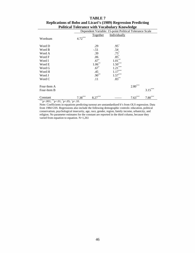
46
TABLE 7
Replications of Bobo and Licari’s (1989) Regression Predicting Political Tolerance with Vocabulary Knowledge
Dependent Variable: 15-point Political Tolerance Scale Together Individually
Wordsum 4.72*** Word D .29 .95+ Word B -.51 .54 Word A .39 .75* Word F .06 .85* Word I .67* 1.01** Word E 1.06** 1.50*** Word G .67* 1.21*** Word H .45 1.17*** Word J .90** 1.57*** Word C .11 .83** Four-Item A 2.80*** Four-Item B 3.15***
Constant 7.38*** 8.27*** ⎯⎯ 7.63*** 7.80***
***p<.001; **p<.01; *p<.05; +p<.10. Note: Coefficients in equations predicting turnout are unstandardized b’s from OLS regression. Data from 1984 GSS. Regressions also include the following demographic controls: education, political conservatism, psychological insecurity, age, race, gender, region, family income, urbanicity, and religion. No parameter estimates for the constant are reported in the third column, because they varied from equation to equation. N=1,261
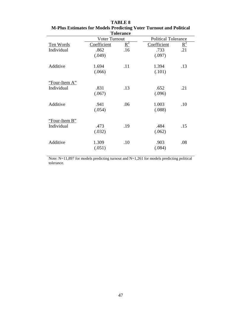
47
TABLE 8
M-Plus Estimates for Models Predicting Voter Turnout and Political Tolerance
Voter Turnout Political Tolerance Ten Words Coefficient R2 Coefficient R2 Individual .862
(.049) .16 .733
(.097)
.21
Additive 1.694 (.066)
.11 1.394 (.101)
.13
“Four-Item A” Individual .831
(.067) .13 .652
(.096)
.21
Additive .941 (.054)
.06 1.003 (.088)
.10
“Four-Item B” Individual .473
(.032) .19 .484
(.062)
.15
Additive 1.309 (.051)
.10 .903 (.084)
.08
Note: N=11,897 for models predicting turnout and N=1,261 for models predicting political tolerance.

48
TABLE 9 Proposals for New Words to be Added to the General Social Survey
IRT Parameters from Lightspeed Research Data
Lightspeed Research General Social Survey Discrimination Difficulty Guessing Current Words Word D 96.7% 93.3% 2.84 -2.24 .15 Word B 95.7 92.8 2.66 -2.34 .16 Word A 88.0 81.9 .92 -2.83 .18 Word F 94.6 78.7 2.67 -2.05 .16 Word I 82.3 78.0 .96 -1.88 .18 Word E 86.1 72.0 2.74 -1.48 .11 Word G 39.6 33.6 1.85 .23 .08 Word H 33.0 29.3 3.48 .44 .13 Word J 37.5 23.2 2.49 .33 .06 Word C 27.7 22.4 1.64 .80 .08 Proposed Additional Words
Lightspeed Research (Actual)
Lightspeed Research (Corrected)
New Word 1 92.1% 84.3% 2.61 -1.90 .17 New Word 2 91.6 83.8 2.24 -2.19 .14 New Word 3 88.2 80.4 1.54 -1.95 .14 New Word 4 86.6 78.8 1.01 -2.39 .17 New Word 5 84.9 77.1 2.31 -1.59 .15 New Word 6 83.8 76.0 .87 -2.29 .15 New Word 7 76.4 68.7 1.50 -1.29 .13 New Word 8 71.6 64.0 2.07 -.97 .09 New Word 9 67.0 59.4 2.47 -.62 .23 New Word 10 65.6 58.0 1.21 -.95 .11 New Word 11 60.8 53.3 1.80 -.53 .16 New Word 12 59.5 52.0 2.48 -.43 .13 New Word 13 57.7 50.2 .59 -.37 .11 New Word 14 57.6 50.1 1.94 -.37 .10 New Word 15 57.5 50.0 1.37 -.43 .11 New Word 16 56.4 48.9 2.29 -.43 .11 New Word 17 54.7 47.2 1.10 -.19 .12 New Word 18 51.7 44.3 1.65 -.32 .06 New Word 19 32.5 25.3 .64 1.95 .13 New Word 20 31.7 24.5 2.48 .67 .10 New Word 21 29.2 22.0 1.86 1.09 .19 New Word 22 28.2 21.0 3.19 .49 .05 New Word 23 23.4 16.3 .60 2.61 .10
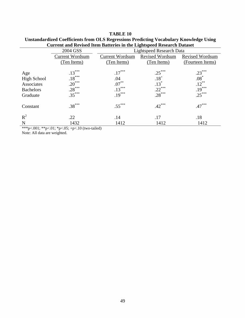
49
TABLE 10 Unstandardized Coefficients from OLS Regressions Predicting Vocabulary Knowledge Using
Current and Revised Item Batteries in the Lightspeed Research Dataset 2004 GSS Lightspeed Research Data Current Wordsum
(Ten Items) Current Wordsum
(Ten Items) Revised Wordsum
(Ten Items) Revised Wordsum (Fourteen Items)
Age .13*** .17*** .25*** .23*** High School .18*** .04 .18+ .08* Associates .20*** .07** .13* .12** Bachelors .28*** .13*** .22*** .19*** Graduate .35*** .19*** .28*** .25*** Constant .38*** .55*** .42*** .47*** R2 .22 .14 .17 .18 N 1432 1412 1412 1412 ***p<.001; **p<.01; *p<.05; +p<.10 (two-tailed) Note: All data are weighted.

50
TABLE 11 M-Plus Estimates for Models Predicting Vocabulary Knowledge Using Current and Revised Item Batteries in the Lightspeed Research Dataset
Current Wordsum (Ten Items)
Revised Wordsum (Ten Items)
Revised Wordsum (Fourteen Items)
Age .087 (.014)
.098 (.014)
.089 (.013)
High School .026 (.017)
.040 (.014)
.037 (.014)
Associates .035 (.018)
.052 (.015)
.046 (.015)
Bachelors .061 (.019)
.075 (.016)
.072 (.016)
Graduate .084 (.020)
.091 (.018)
.090 (.017)
R2 .15 .21 .19 Note: N=1,412. All data are weighted.

51
TABLE 12 Cross-Tabulation of Scores from Revised Wordsum (Fourteen Items) against Current Wordsum (Ten Items)
10 9 8 7 6 5 4 3 2 1 0 14 12.7% .0% .0% .0% .0% .0% .0% .0% .0% .0% .0% 13 .7 13.1 .0 .0 .0 .0 .0 .0 .0 .0 .0 12 .2 1.6 9.6 .0 .0 .0 .0 .0 .0 .0 .0 11 .0 .4 5.3 6.9 .0 .0 .0 .0 .0 .0 .0 10 .0 .1 1.5 5.7 4.2 .0 .0 .0 .0 .0 .0 9 .0 .0 .5 3.9 6.2 .6 .0 .0 .0 .0 .0 8 .0 .0 .0 1.8 5.3 1.9 .3 .0 .0 .0 .0 7 .0 .0 .0 .4 3.5 1.9 .4 .0 .0 .0 .0 6 .0 .0 .0 .0 1.9 2.6 .9 .1 .0 .0 .0 5 .0 .0 .0 .0 .0 1.5 1.2 .1 .0 .0 .0 4 .0 .0 .0 .0 .0 .0 .8 .6 .0 .0 .0 3 .0 .0 .0 .0 .0 .0 .0 .5 .1 .1 .0 2 .0 .0 .0 .0 .0 .0 .0 .0 .3 .0 .0 1 .0 .0 .0 .0 .0 .0 .0 .0 .0 .3 .1 0 .0 .0 .0 .0 .0 .0 .0 .0 .0 .0 .4

52
1975 1980 1985 1990 1995 2000
6070
8090
100
Figure 1: Frequencies of Correct Responses Over Time (Easy Words)
Year
% C
orre
ct
Word DWord BWord AWord FWord IWord E

53
1975 1980 1985 1990 1995 2000
1015
2025
3035
40
Figure 2: Frequencies of Correct Responses Over Time (Hard Words)
Year
% C
orre
ct
Word GWord HWord JWord C
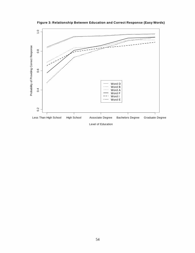
54
0.2
0.4
0.6
0.8
1.0
Figure 3: Relationship Between Education and Correct Response (Easy Words)
Level of Education
Prob
abilit
y of
Pro
vidi
ng C
orre
ct R
espo
nse
Less Than High School High School Associate Degree Bachelors Degree Graduate Degree
Word DWord BWord AWord FWord IWord E

55
0.0
0.2
0.4
0.6
0.8
Figure 4: Relationship Between Education and Correct Response (Hard Words)
Level of Education
Prob
abilit
y of
Pro
vidi
ng C
orre
ct R
espo
nse
Less Than High School High School Associate Degree Bachelors Degree Graduate Degree
Word GWord HWord JWord C

56
Figure 5: Distribution of Vocabulary Knowledge Scores for Current and Revised Item Batteries in GSS and Lightspeed Research Data
05
1015
20P
erce
ntag
e of
Res
pond
ents
0 1 2 3 4 5 6 7 8 9 10Number of Correct Responses
GSS--Current Wordsum (Ten Items)Distribution of Vocabulary Scores
05
1015
20P
erce
ntag
e of
Res
pond
ents
0 1 2 3 4 5 6 7 8 9 10Number of Correct Responses
Lightspeed--Current Wordsum (Ten Items)Distribution of Vocabulary Scores
05
1015
20P
erce
ntag
e of
Res
pond
ents
0 2 4 6 8 10Number of Correct Responses
Lightspeed--Revised Wordsum (Ten Items)Distribution of Vocabulary Scores
05
1015
Per
cent
age
of R
espo
nden
ts
0 1 2 3 4 5 6 7 8 9 10 11 12 13 14Number of Correct Responses
Lightspeed--Revised Wordsum (Fourteen Items)Distribution of Vocabulary Scores

57
Figure 6: Test Information Functions for Current and Revised Item Batteries in Lightspeed Research Data
-3 -2 -1 0 1 2 30
1
2
3
4
5
6
Scale Score
Info
rmat
ion
Subtest: TEST0001
0
0 .64
1 .28
1 .92
2 .56
3 .20
Standard Error
Test Information Curve, Lightspeed—Current Wordsum (Ten Items)
-3 -2 -1 0 1 2 30
1
2
3
4
5
6
7
Scale Score
Info
rmat
ion
Subtest: TEST0001
0
0 .63
1 .27
1 .90
2 .53
3 .16
Standard Error
Test Information Curve, Lightspeed—Revised Wordsum (Fourteen Items)
-3 -2 -1 0 1 2 30
1
2
3
4
5
6
Scale Score
Info
rmat
ion
Subtest: TEST0001
0
1 .13
2 .26
3 .39
4 .52
5 .65
Standard Error
Test Information Curve, Lightspeed—Revised Wordsum (Ten Items)
58
References
Alwin, Duane F. 1991. “Family of Origin and Cohort Differences in Verbal Ability.” American
Sociological Review. 56(5): 625-638.
Alwin, Duane F. and Ryan J. McCammon. 1999. “Aging Versus Cohort Interpretations of
Intercohort Differences in GSS Vocabulary Scores.” American Sociological Review.
64(2): 272-286.
Arthur, John A. and Charles E. Case. 1994. “Race, Class, and Support for Police Use of Force.”
Crime, Law, and Social Change. 21(2): 167-182.
Baker, Frank B. 2004. Item Theory Response: Parameter Estimation Techniques (2nd ed.). New
York: Marcel Dekker.
Bailey, Kent. G. and Edward J. Federman. 1979. “Factor Analysis of Breadth and Depth
Dimensions on Wechsler’s Similarities and Vocabulary Subscales.” Journal of Clinical
Psychology. 35(2): 341-345.
Beck, N. C., D. Tucker, R. Frank, J. Parker, R. Lake, S. Thomas, W. Lichty, E. Horwitz,
B. Horwitz, and F. Merritt.1989. ”The latent factor structure of the WAIS-R: A factor
analysis of individual item responses.” Journal of Clinical Psychology. 45(2): 281-293.
Blake, Judith. 1989. Family Size and Achievement. Berkeley: University of California Press.
Bobo, Lawrence and Frederick C. Licari. 1989. “Education and Political Tolerance: Testing the
Effects of Cognitive Sophistication and Target Group Affect.” Public Opinion Quarterly.
53(3): 285-308.
Bock, R. Darrell and Murray Aitken. 1981. “Marginal Maximum Likelihood Estimation of Item
Parameters: Application of an EM algorithm.” Psychometrika. 46(4): 443- 459.
Bowles, Ryan P., Kevin J. Grimm, and John J. McArdle. 2005. "A Structural Factor Analysis of
59
Vocabulary Knowledge and Relations to Age." Journal of Gerontology: Psychological
Sciences and Social Sciences. 60(5): 234-241.
Brainerd, Charles J., and Valerie F. Reyna. 1992. "Explaining ‘Memory Free’ Reasoning."
Psychological Science. 3(6): 332-339.
Case, Charles E., Andrew M. Greeley, and Stephen Fuchs. 1989. "Social Determinants of Racial
Prejudice." Sociological Perspectives. 32(4): 469-483.
Cattell, Raymond B. 1963. "Theory of Fluid and Crystallized Intelligence: a Critical
Experiment." Journal of Educational Psychology. 54(1): 1-22.
Cattell, Raymond B. 1987. Intelligence: Its Structure, Growth, and Action. Amsterdam: Elsevier.
Cattell, Raymond B. 1998. "Where is Intelligence? Some Answers from the Triadic Theory." In
John J. McArdle & Richard W. Woodcock (Eds.), Human Cognitive Abilities in Theory
and Practice. Mahwah, NJ: Erlbaum.
Embretson, Susan E., and Reise, Steven P. 2000. Item Response Theory for Psychologists.
Mahwah, NJ: Erlbaum.
Gardner, Howard. 1993. Frames of Mind: The Theory of Multiple Intelligences. New York:
Basic Books.
Glenn, Norval D. 1994. "Television Watching, Newspaper Reading, and Cohort Differences in
Verbal Ability." Sociology of Education. 67(3): 216-230.
Glenn, Norval D. and L. Hill, Jr. 1977. “Rural-Urban Differences in Attitudes and Behavior in
the United States.” Annals of the American Academy of Political and Social Science.
429(1): 36-50.
Hauser, Seth M. 2000. “Education, Ability and Civic Engagement in the Contemporary United
States.” Social Science Research. 29(4): 556-582.

60
Hauser, Robert M. and Min-Hsiung Huang. 1997. “Verbal Ability and Socioeconomic Success:
A Trend Analysis.” Social Science Research. 26(3): 331-376.
Herrnstein, Richard J. and Charles Murray. 1994. The Bell Curve. New York: Free Press.
Horn, J. L. and Roger B. Cattell. 1967. “Age Differences in Fluid and Crystallized Intelligence.”
Acta Psychologica. 26(2): 107-129.
Hyman, Herbert H., Charles R.Wright, and John S. Reed. 1975. The Enduring Effects of
Education. Chicago: The University of Chicago Press.
Junn, Jane. 1991. Participation and Political Knowledge. In W. Crotty (Ed.), Political
Participation and American Democracy. New York: Greenwood Press.
Krosnick, Jon A. and Duane F. Alwin. 1987. “An Evaluation of a Cognitive Theory of Response
Order Effects in Survey Measurement.” Public Opinion Quarterly. 51(2): 201-219.
Lewis, Gregory B. 1990. “In Search of the Machiavellian Milquetoasts: Comparing Attitudes of
Bureaucrats and Ordinary People.” Public Administration Review. 50(2): 220-227.
Loeb, Susanna and John Bound. 1996. “The Effect of Measured School Inputs on Academic
Achievement: Evidence from the 1920s, 1930s, and 1940s Birth Cohorts.” The Review of
Economics and Statistics. 78(4): 653-664.
Lynn, Richard and Marilyn Van Court. 2004. "New Evidence of Dysgenic Fertility for
Intelligence in the United States." Intelligence. 32(22): 193-201.
Raven, John C. 1982. Revised Manual for Raven's Progressive Matrices and Vocabulary Scale.
Windsor, UK: NFER Nelson.
Rempel, Michael. 1997. "Contemporary Ideological Cleavages in the United States." In T.N.
Clark and M. Rempel (Eds.), Citizen Politics on Post-Industrial Societies. Boulder, CO:
Westview Press.
61
Morgan, Michael. 1986. "Television and Adults' Verbal Intelligence." Journalism Quarterly.
63(3): 537-541.
Miner, John. B. 1957. Intelligence in the United States: A Survey with Conclusions for
Manpower Utilization in Education and Employment. New York: Springer.
Nash, Jeffrey. E. 1991. "Race and Words: A Note on the Sociolinguistic Divisiveness of Race in
American Society." Sociological Inquiry. 61(2): 252-262.
National Opinion Research Center. 1966. Study SRS-889A. Chicago: NORC.
Nelson, Michael J. and Ewen C. Denney. 1960. The Nelson-Denney Reading Test (revised by
James I. Brown). Boston: Houghton Mifflin.
Schaie, K. Warner. 1996. Intellectual Development in Adulthood: The Seattle Longitudinal
Study. New York: Cambridge University Press.
Skrondal, Anders and Sophia Rabe-Hesketh. 2004. Generalized Latent Variable Modeling:
Multilevel, Longitudinal, and Structural Equation Models. Boca Raton, FL: Chapman &
Hall/CRC.
Shipley, Walter C. 1946. Institute of Living Scale. Los Angeles: Western Psychological Services.
Sigelman, Lee. 1981. “Is Ignorance Bliss? A Reconstruction of the Folk Wisdom.” Human
Relations. 34(4): 965-974.
Smith, Tom W. 1981. “Contradictions on the Abortion Scale.” GSS Methodological Report, 19.
Smith, Tom W. 1992. “A Methodological Analysis of the Sexual Behavior Questions on the
General Social Surveys.” Journal of Official Statistics. 8(3): 309-325.
Smith, Tom W. 1993. “The Relationship of Age to Education Across Time.” Social Science
Research. 22(3): 300-311.
Thorndike, Robert L. 1942. “Two Screening Tests of Verbal Intelligence.” Journal of Applied

62
Psychology. 26: 128-135.
Thorndike, Robert L. and Gallup, George H. 1944. “Verbal Intelligence in the American Adult.”
Journal of General Psychology. 30: 75-85.
Van Court, M., & Bean, F. D. 1985. “Intelligence and Fertility in the United States: 1912-1982.”
Intelligence. 9(1): 23-32.
Verba. Sidney, Kay Lehman Schlozman, and Henry E. Brady. 1985. Voice and Equality: Civic
Voluntarism in American Politics. Cambridge: Harvard University Press.
Walberg, Herbert J. and Thomas Weinstein. 1984. “Adult Outcomes of Connections,
Certification, and Verbal Competence.” Journal of Educational Research. 77(4): 207-
212.
Weakliem, David, Julia McQullan, and Tracy Schauer. 1995. “Toward Meritocracy? Changing
Social-Class Differences in Intellectual Ability.” Sociology of Education. 68(4): 271-286.
Wechsler, David. 1981. WAIS-R manual. New York: The Psychological Corporation.
Wilson, James A. and Walter R. Gove. 1999a. “The Age-Period-Cohort Conundrum and Verbal
Ability: Empirical Relationships and their Interpretation: Reply to Glenn and to Alwin
and McCammon.” American Sociological Review. 64(2): 287-302.
Wilson, James A. and Walter R. Gove. 1999b. “The Intercohort Decline in Verbal
Ability: Does it Exist?” American Sociological Review. 64(2): 253-266.
Wolfle, Lee M. 1980. “The Enduring Effects of Education on Verbal Skills.” Sociology of
Education. 53(3): 104-114.
Zajonc, R. B. and Gregory B. Markus. 1975. “Birth Order and Intellectual Development.”
Psychological Review. 82(1): 74-88.

63
Zimowski, M. F., Muraki, E., Mislevy, R. J., & Bock, R. D. (1996). BILOG-MG [Computer
software]. Chicago: Scientific Software International.