Embed Size (px)
Citation preview
Exploiting the Magnetic Origin of Solar Activity in Forecasting
Thermospheric Density Variations
Harry Warren
Naval Research Laboratory, Space Science Division, Washington, DC
John Emmert
Naval Research Laboratory, Space Science Division, Washington, DC
Abstract A detailed understanding of solar irradiance and its variability at extreme ultraviolet (EUV)
wavelengths is required to model thermospheric density and to specify and forecast satellite drag. Current
operational models rely on forecasts of proxies for solar activity based on autoregression. The forecasts from
these models generally degrade to climatology after only a few days. Solar magnetic fields are ultimately
responsible for variations in the EUV irradiance. The evolution of solar magnetic fields is well understood
and results from a combination of solar rotation, diffusion, meridional flow, and magnetic flux emergence.
In this presentation we review the current state of autoregressive proxy models and compare their forecast
skill against new activity models based on magnetic flux transport.
1. Introduction
The influence of the Sun’s extreme ultraviolet radiation (EUV, 50–1200 A) on the Earth’s upper atmo-
sphere is perhaps the most dramatic of all the Sun-Earth connections. The solar irradiance at these wave-
lengths is directly coupled to solar activity and is strongly modulated by the 11-year sunspot cycle. Solar
EUV radiation is deposited in the Earth’s atmosphere at heights above about 100 km where the densities are
low. The coupling of the highly variable solar EUV emission to the Earth’s tenuous upper atmosphere leads
to dramatic variations in the thermodynamics, chemical composition, and ionization of the Earth’s upper
atmosphere over the solar cycle. The maximum temperature of the thermosphere, for example, typically
rises by about 500 K (750 to 1250 K) from solar minimum to solar maximum. Both the neutral and elec-
tron density in this region can change by more than an order of magnitude during a typical solar cycle [for
reviews see 6, 9].
The close connection between solar variability at these wavelengths and thermospheric density means
that accurately specifying and forecasting satellite drag requires a detailed understanding of the solar EUV
irradiance. Unfortunately, establishing and monitoring the absolute radiometric calibration of EUV instru-
ments is difficult and much of our quantitative understanding of the solar EUV irradiance and its variability
remains uncertain. For example, it is not clear if the unusually low values for various irradiance measure-
ments taken during the recent solar minimum reflect real changes in the solar atmosphere or are simply
instrumental problems. The Solar EUV Monitor (SEM) on SOHO recorded a 15% reduction in the irradi-
ance near 304 A between the 1996 and 2008 minima [18], but the behavior of F10.7 and the Mg II core-to-
wing ratio, proxies for solar activity, suggests that the irradiance during the two solar minima should differ
by only a few percent [2, 14]. In the absence of continuous and well calibrated solar spectral irradiance
measurements, models of thermospheric density rely on proxies for solar activity.
In this paper we explore the use of solar magnetic field measurements as both the basis of solar EUV
irradiance variability models as well as for use in forecasting irradiance variability. Spatially resolved mea-
surements of solar radiance are well correlated with the magnitude of the underlying magnetic field. This is
the so-called “flux-luminosity” relationship [e.g., 12, 3], which holds in conditions ranging from the quiet
Sun to the most active stars [11]. This concept has already been applied to models of the total solar irra-
diance [e.g., the SATIRE-S model 1]) and is likely to form the basis of future irradiance models at other
wavelengths. Furthermore, the evolution of solar magnetic fields is generally well understood and results
from a combination of solar rotation, diffusion, meridional flow, and magnetic flux emergence [for a review
see 10]. Thus it should be possible to make accurate forecasts of solar magnetic fields and proxies for solar
activity related to them [see 4, for the application of this idea to forecasting F10.7 ]. Current forecasts of so-
lar activity are often based on polynomial extrapolations (or autoregression) and their performance degrades
quickly. Our goal is to make quantitative comparisons between models based on autoregression and models
based on magnetic flux transport.
2. Autoregressive Forecast Models
The 27 day rotational period of the sun leads to a quasi-periodic modulation in the solar irradiance at all
wavelengths. Current forecasts of proxies for solar activity often use autoregression to predict the amplitude
of this quasi-periodic signature [e.g. 16, 8]. This approach makes use of a least-squares polynomial fit of
“past” data to “future” data. That is, the observations are fit to an equation of the form f+n = c + a0f0 +a−1f−1 + a−2f−2 + · · ·, where f+n is the value of the proxy n days in the future from a given date and the
right hand side of the equation represents the values of the proxy on the date of interest and before. Here we
address several basic questions, such as what is the optimal amount of past data to include? How does the
forecast error increase with the length of the forecast? and How does autoregression compare with simple
reference models?
For this analysis we use the daily F10.7 observations collected over the past 6 solar cycles (January
1, 1954 to June 30, 2014). Note that of these 22,066 observations we have generated spline interpolated
values for 168 (0.8%) missing observations. Most of these missing data points are from the 1950’s. This
period is included because it represents the highest levels of solar activity observed over the past several
hundred years. This data was randomly divided into a training set comprising 60% of the observations, and
a validation set, which contains the remaining 40% of the data. The training data is used to determine the
coefficients for the polynomial fit while the validation data is used to estimate the forecast error and skill.
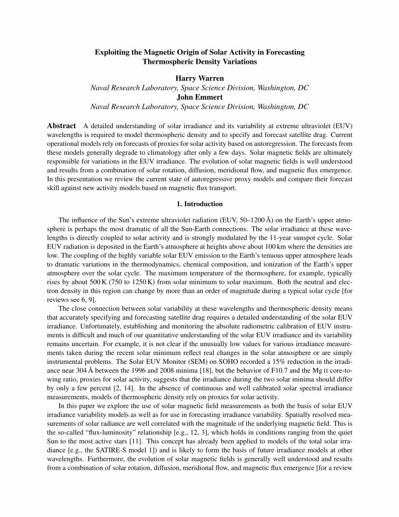
We considered forecasts of 1 to 45 days using ensembles of between 1 and 108 past data values. For
each model we computed the root-mean-square-error (RMSE) from the validation set as a function of fore-
cast day and model complexity. The lowest forecast error is generally achieved for models with the most
coefficients, although we found that there is little marginal benefit to considering more than about 30 previ-
ous observations. For the remainder of this paper we present results from models that use 108 previous data
points. The RMSE as a function of forecast day for this case is shown in Fig. 1. Here we see that the RMSE
rises rapidly for about 10 days and then asymptotes.
To evaluate the skill of the autoregressive forecast we compared it with two very simple reference fore-
cast models: “persistence” — predicting that the last measured value will be observed for the next 45 days,
and “climatology” — predicting that the average value from the previous 81 days will be observed over the
next 45 days. We compute the model skill using
Skill = 1−MSE(model)
MSE(reference). (1)
This comparisons shows the expected result, with the persistence reference model performing similarly to
autoregression for very short periods, and autoregression converging to climatology over long periods. The
peak skill in the autoregression model (0.4) is achieved at 6 days.
Note that the forecast and skill reported here are for the entire data set. These metrics vary with the
solar cycle. At high levels of solar activity RMSE increases, but skill remains relatively high. At low levels
of solar activity RMSE decreases, but since there is very little modulation in the irradiance and the simple
reference models perform well, the skill of the forecast also falls.
We have repeated this exercise for the S10 proxy, which is simply a scaled version of the broad band
irradiance measured by the SEM on SOHO [15]. These results, which are also shown in Fig. 1, are similar
to those obtained for f10.7, except that the RMSE for the autoregressive forecast are about 50% smaller.
0
10
20
30
RM
S E
rror
%
F10.7
81−Day MeanPersistenceRegression
0 10 20 30 40Forecast Day
0.0
0.2
0.4
0.6
0.8
1.0
Ski
ll
Regression vs. PersistenceRegression vs. 81−Day Mean
0
10
20
30
RM
S E
rror
(%
)
S10 RegressionPersistence
81−Day Mean
0 10 20 30 40Forecast Day
0.0
0.2
0.4
0.6
0.8
1.0
Ski
ll
Regression vs. PersistenceRegression vs. 81−Day Mean
Figure 1: RMSE and forecast skill as a function of forecast day for autoregressive models of two proxies for
solar activity. The F10.7 cm radio flux is shown in the top panela and S10 is shown in the bottom panels.
The autoregressive models are compared against simple models of persistence and the 81-day running mean.
For both proxies forecast skill peaks at about 6 days.
As we will demonstrate in the next section, this out-performance is likely due to the fact that S10 is more
closely tied to emission from the lowest layers of the solar atmosphere.
3. Using the Solar Magnetic Field as a Proxy for Solar Activity
Several recent irradiance models of the total solar irradiance have used spatially resolved magnetic field
measurements as an input [e.g., SATIRE-S 1, 5]. The basic assumption in these models is that only changes
in the surface magnetic fields impact the solar irradiance on time scales greater than one day [e.g., 7]. Here
07−Oct−03 00:03:03
12−Oct−03 15:59:03
18−Oct−03 15:59:03
24−Oct−03 07:59:03
30−Oct−03 08:00:03
0
5.0•106
1.0•107
1.5•107
2.0•107
total EIT Intensity
12−Oct 17−Oct 22−Oct 27−Oct 01−NovStart Time (07−Oct−03 00:03:03)
0
5.0•1022
1.0•1023
1.5•1023
total MDI Unsigned Flux
0
5.0•106
1.0•107
1.5•107
2.0•107
tota
l EIT
Inte
nsity
(D
N/s
)
correlation = 0.96
0 5.0•1022 1.0•1023 1.5•1023
total MDI Unsigned Flux (MX)
−60−40
−20
0
20
40
60
% D
iffer
ence
σ = 6.8%
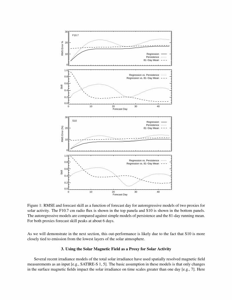
Figure 2: Observations of radiance and magnetic field at disk center. These observations illustrate the strong
correlation between the integrated radiance and the total unsigned magnetic flux. The top panels show
examples of the radial magnetic field measured with the Michelson Doppler Imager (MDI) and the 304 A
radiance from the EUV Imaging Telescope (EIT) measured at disk center. The bottom left panels show
the corresponding time series. The bottom right panels show a linear regression between the total unsigned
magnetic flux and the total radiance in the field of view. The residuals between the simple linear model and
the observed total radiance is also shown.
we illustrate the robustness of this assumption for EUV emission from small regions of the solar disk so we
can discuss this in terms of a flux-radiance relationship. We also show that it is possible to use the magnetic
field integrated over the disk as a replacement for other proxies of solar activity.
The relationship between the radiance and the unsigned magnetic flux is illustrated in Fig. 2. The upper
panels in this figure show the central portion of the solar disk from several MDI magnetograms (top) and EIT
images at 304 A (bottom) from October 7 through November 5, 2003. This period is one of particularly high
solar activity and is a challenge for any modeling. The two panels on the lower left show the times series
of the EIT 304 A emission and unsigned magnetic flux integrated over this region (Φr =∑
|Br| ·A, where
Br is the flux density in Gauss in a pixel and A is the pixel area). The strong correlation is clearly shown by
these two time series. A scatter plot of these values is shown in the lower right portion of Fig. 2 along with
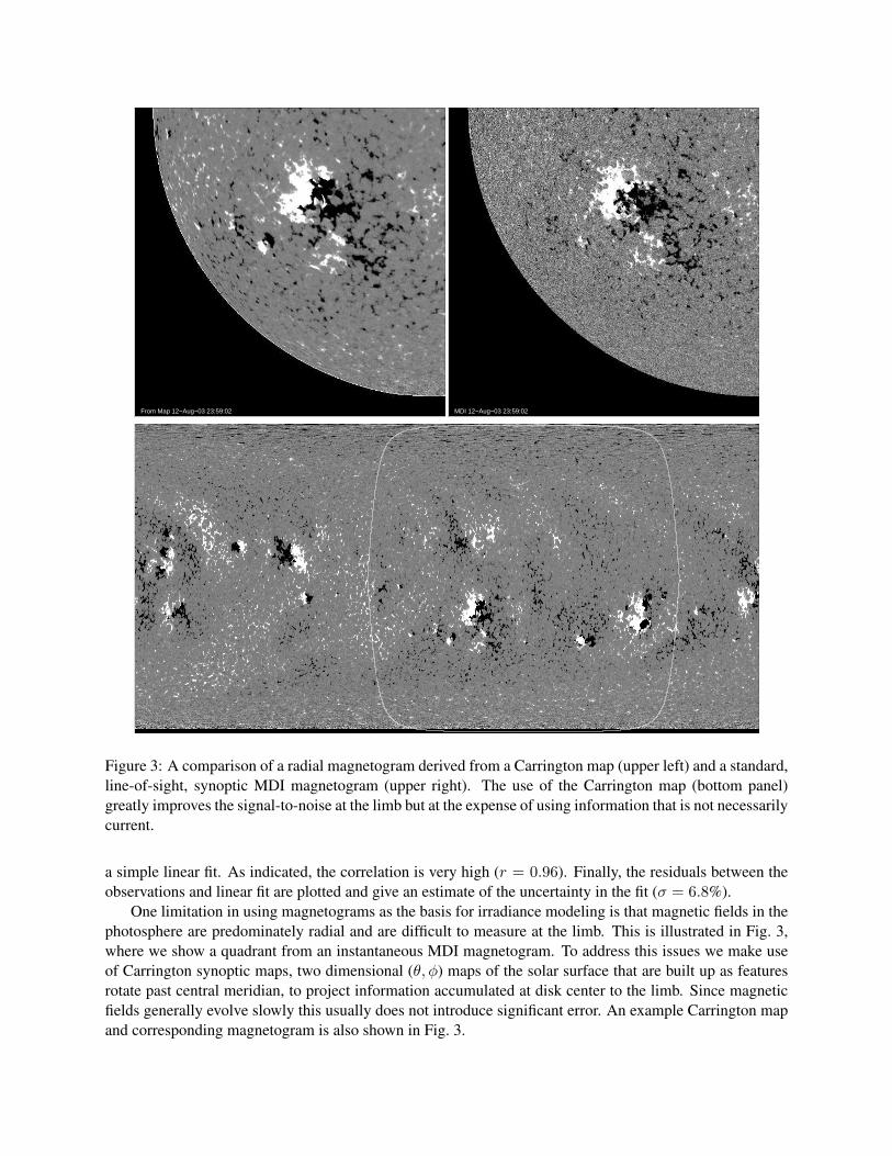
From Map 12−Aug−03 23:59:02
MDI 12−Aug−03 23:59:02
Figure 3: A comparison of a radial magnetogram derived from a Carrington map (upper left) and a standard,
line-of-sight, synoptic MDI magnetogram (upper right). The use of the Carrington map (bottom panel)
greatly improves the signal-to-noise at the limb but at the expense of using information that is not necessarily
current.
a simple linear fit. As indicated, the correlation is very high (r = 0.96). Finally, the residuals between the
observations and linear fit are plotted and give an estimate of the uncertainty in the fit (σ = 6.8%).
One limitation in using magnetograms as the basis for irradiance modeling is that magnetic fields in the
photosphere are predominately radial and are difficult to measure at the limb. This is illustrated in Fig. 3,
where we show a quadrant from an instantaneous MDI magnetogram. To address this issues we make use
of Carrington synoptic maps, two dimensional (θ, φ) maps of the solar surface that are built up as features
rotate past central meridian, to project information accumulated at disk center to the limb. Since magnetic
fields generally evolve slowly this usually does not introduce significant error. An example Carrington map
and corresponding magnetogram is also shown in Fig. 3.
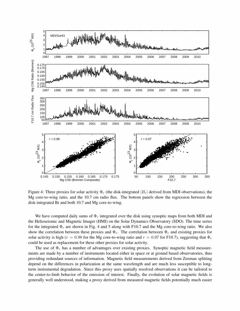
1997 1998 1999 2000 2001 2002 2003 2004 2005 2006 2007 2008 2009 201001
2
3
45
Φr (
1023
MX
)MDI/SoHO
1997 1998 1999 2000 2001 2002 2003 2004 2005 2006 2007 2008 2009 20100.1450.1500.1550.1600.1650.1700.175
Mg
C/W
Rat
io (
Bre
men
)
1997 1998 1999 2000 2001 2002 2003 2004 2005 2006 2007 2008 2009 201050
100150200250300350
F10
.7 c
m R
adio
Flu
x
0.145 0.150 0.155 0.160 0.165 0.170 0.175Mg C/W (Bremen Composite)
0
1
2
3
4
5
Φr (
1023
MX
)
r = 0.98
50 100 150 200 250 300 350F10.7
0
1
2
3
4
5
Φr (
1023
MX
)
r = 0.97
Figure 4: Three proxies for solar activity Φr (the disk-integrated |Br| derived from MDI observations), the
Mg core-to-wing ratio, and the 10.7 cm radio flux. The bottom panels show the regression between the
disk-integrated Br and both 10.7 and Mg core-to-wing.
We have computed daily sums of Φr integrated over the disk using synoptic maps from both MDI and
the Helioseismic and Magnetic Imager (HMI) on the Solar Dynamics Observatory (SDO). The time series
for the integrated Φr are shown in Fig. 4 and 5 along with F10.7 and the Mg core-to-wing ratio. We also
show the correlation between these proxies and Φr. The correlation between Φr and existing proxies for
solar activity is high (r = 0.98 for the Mg core-to-wing ratio and r = 0.97 for F10.7), suggesting that Φr
could be used as replacement for these other proxies for solar activity.
The use of Φr has a number of advantages over existing proxies. Synoptic magnetic field measure-
ments are made by a number of instruments located either in space or at ground based observatories, thus
providing redundant sources of information. Magnetic field measurements derived from Zeeman splitting
depend on the differences in polarization at the same wavelength and are much less susceptible to long-
term instrumental degradation. Since this proxy uses spatially resolved observations it can be tailored to
the center-to-limb behavior of the emission of interest. Finally, the evolution of solar magnetic fields is
generally well understood, making a proxy derived from measured magnetic fields potentially much easier
2010 2011 2012 2013 20140
1
2
3HMI/SDO
Φr (
1023
MX
)
2010 2011 2012 2013 20140.1450.1500.1550.1600.1650.1700.175
Mg
C/W
Rat
io
2010 2011 2012 2013 201450
100150200250300350
F10
.7 c
m R
adio
Flu
x
0.145 0.150 0.155 0.160 0.165 0.170 0.175Mg C/W (Bremen Composite)
0
1
2
3
4
Φr (
1023
MX
)
r = 0.97
50 100 150 200 250 300F10.7
0
1
2
3
Φr (
1023
MX
)
r = 0.90
Figure 5: The same as Fig. 4, but for Φr derived from HMI observations of the magnetic field. The dotted
line in the top panel shows the results from MDI for this period.
to forecast.
4. Magnetic Flux Transport and Forecasting Magnetic Activity
The evolution of magnetic fields on the solar surface can be described by a two-dimensional convection-
diffusion equation:
∂Br
∂t= −ω(θ)
∂Br
∂φ−
1
R⊙ sin θ
∂
∂θ[v(θ)Br sin θ] + κ∇2
⊥Br + S (2)
where ω(θ) is the differential rotation rate, v(θ) is the meridional flow velocity, κ is the diffusion rate, and
S is the flux emergence rate [see 10, for a review].
We have implemented a discrete flux transport model similar to those of Wang and Sheeley [17], Worden
and Harvey [19], and Schrijver [13], but that is optimized for use with new observations at higher spatial
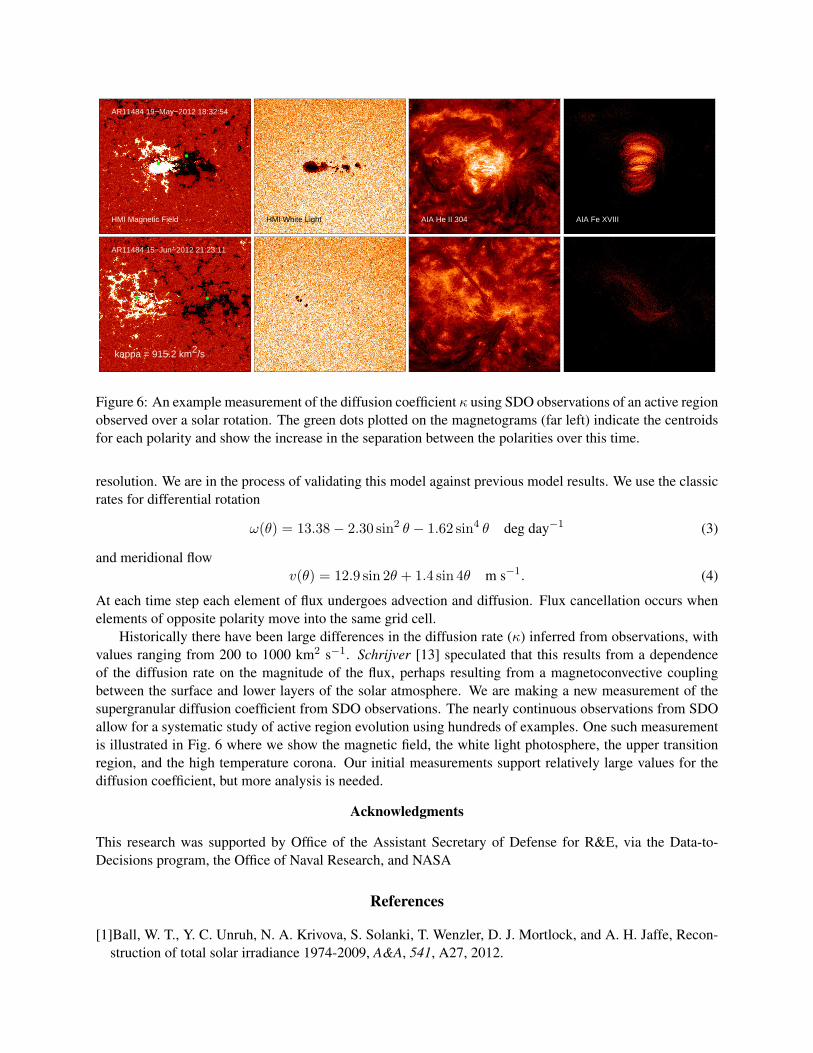
HMI Magnetic Field
AR11484 19−May−2012 18:32:54
HMI White Light
AIA He II 304
AIA Fe XVIII
kappa = 915.2 km2/s
AR11484 15−Jun−2012 21:23:11
Figure 6: An example measurement of the diffusion coefficient κ using SDO observations of an active region
observed over a solar rotation. The green dots plotted on the magnetograms (far left) indicate the centroids
for each polarity and show the increase in the separation between the polarities over this time.
resolution. We are in the process of validating this model against previous model results. We use the classic
rates for differential rotation
ω(θ) = 13.38− 2.30 sin2 θ − 1.62 sin4 θ deg day−1 (3)
and meridional flow
v(θ) = 12.9 sin 2θ + 1.4 sin 4θ m s−1. (4)
At each time step each element of flux undergoes advection and diffusion. Flux cancellation occurs when
elements of opposite polarity move into the same grid cell.
Historically there have been large differences in the diffusion rate (κ) inferred from observations, with
values ranging from 200 to 1000 km2 s−1. Schrijver [13] speculated that this results from a dependence
of the diffusion rate on the magnitude of the flux, perhaps resulting from a magnetoconvective coupling
between the surface and lower layers of the solar atmosphere. We are making a new measurement of the
supergranular diffusion coefficient from SDO observations. The nearly continuous observations from SDO
allow for a systematic study of active region evolution using hundreds of examples. One such measurement
is illustrated in Fig. 6 where we show the magnetic field, the white light photosphere, the upper transition
region, and the high temperature corona. Our initial measurements support relatively large values for the
diffusion coefficient, but more analysis is needed.
Acknowledgments
This research was supported by Office of the Assistant Secretary of Defense for R&E, via the Data-to-
Decisions program, the Office of Naval Research, and NASA
References
[1]Ball, W. T., Y. C. Unruh, N. A. Krivova, S. Solanki, T. Wenzler, D. J. Mortlock, and A. H. Jaffe, Recon-
struction of total solar irradiance 1974-2009, A&A, 541, A27, 2012.
[2]Emmert, J. T., J. L. Lean, and J. M. Picone, Record-low thermospheric density during the 2008 solar
minimum, Geophys. Res. Lett., 37, 12,102, 2010.
[3]Fisher, G. H., D. W. Longcope, T. R. Metcalf, and A. A. Pevtsov, Coronal Heating in Active Regions as
a Function of Global Magnetic Variables, ApJ, 508, 885–898, 1998.
[4]Henney, C. J., W. A. Toussaint, S. M. White, and C. N. Arge, Forecasting F10.7 with solar magnetic flux
transport modeling, Space Weather, 10, 2011, 2012.
[5]Krivova, N. A., S. K. Solanki, T. Wenzler, and B. Podlipnik, Reconstruction of solar UV irradiance since
1974, Journal of Geophysical Research (Atmospheres), 114, 0, 2009.
[6]Lean, J., The Sun’s Variable Radiation and Its Relevance For Earth, ARA&A, 35, 33–67, 1997.
[7]Lean, J. L., J. Cook, W. Marquette, and A. Johannesson, Magnetic Sources of the Solar Irradiance Cycle,
ApJ, 492, 390, 1998.
[8]Lean, J. L., J. M. Picone, and J. T. Emmert, Quantitative forecasting of near-term solar activity and upper
atmospheric density, Journal of Geophysical Research (Space Physics), 114, 7301, 2009.
[9]Lean, J. L., T. N. Woods, F. G. Eparvier, R. R. Meier, D. J. Strickland, J. T. Correira, and J. S. Evans,
Solar extreme ultraviolet irradiance: Present, past, and future, Journal of Geophysical Research (Space
Physics), 116, 1102, 2011.
[10]Mackay, D., and A. Yeates, The Sun’s Global Photospheric and Coronal Magnetic Fields: Observations
and Models, Living Reviews in Solar Physics, 9, 6, 2012.
[11]Pevtsov, A. A., G. H. Fisher, L. W. Acton, D. W. Longcope, C. M. Johns-Krull, C. C. Kankelborg, and
T. R. Metcalf, The Relationship Between X-Ray Radiance and Magnetic Flux, ApJ, 598, 1387–1391,
2003.
[12]Schrijver, C. J., Solar active regions - Radiative intensities and large-scale parameters of the magnetic
field, A&A, 180, 241–252, 1987.
[13]Schrijver, C. J., Simulations of the Photospheric Magnetic Activity and Outer Atmospheric Radiative
Losses of Cool Stars Based on Characteristics of the Solar Magnetic Field, ApJ, 547, 475–490, 2001.
[14]Solomon, S. C., L. Qian, L. V. Didkovsky, R. A. Viereck, and T. N. Woods, Causes of low thermospheric
density during the 2007-2009 solar minimum, Journal of Geophysical Research (Space Physics), 116, 0,
2011.
[15]Tobiska, W. K., and S. D. Bouwer, New developments in SOLAR2000 for space research and opera-
tions, Advances in Space Research, 37, 347–358, 2006.
[16]Tobiska, W. K., S. D. Bouwer, and B. R. Bowman, The development of new solar indices for use in
thermospheric density modeling, Journal of Atmospheric and Solar-Terrestrial Physics, 70, 803–819,
2008.
[17]Wang, Y.-M., and N. R. Sheeley, Jr., The rotation of photospheric magnetic fields: A random walk
transport model, ApJ, 430, 399–412, 1994.
[18]Woods, T. N., Irradiance Variations during This Solar Cycle Minimum, in SOHO-23: Understanding a
Peculiar Solar Minimum, edited by S. R. Cranmer, J. T. Hoeksema, and J. L. Kohl, vol. 428 of Astronom-
ical Society of the Pacific Conference Series, p. 63, 2010.
[19]Worden, J., and J. Harvey, An Evolving Synoptic Magnetic Flux map and Implications for the Distribu-
tion of Photospheric Magnetic Flux, Sol. Phys., 195, 247–268, 2000.