Embed Size (px)
Citation preview
Exploiting Local and Global Patch Rarities for Saliency Detection
Ali BorjiUSC
Laurent IttiUSC
Abstract
We introduce a saliency model based on two key ideas.The first one is considering local and global image patchrarities as two complementary processes. The second oneis based on our observation that for different images, oneof the RGB and Lab color spaces outperforms the other insaliency detection. We propose a framework that measurespatch rarities in each color space and combines them ina final map. For each color channel, first, the input im-age is partitioned into non-overlapping patches and theneach patch is represented by a vector of coefficients thatlinearly reconstruct it from a learned dictionary of patchesfrom natural scenes. Next, two measures of saliency (Localand Global) are calculated and fused to indicate saliencyof each patch. Local saliency is distinctiveness of a patchfrom its surrounding patches. Global saliency is the inverseof a patch’s probability of happening over the entire image.The final saliency map is built by normalizing and fusinglocal and global saliency maps of all channels from bothcolor systems. Extensive evaluation over four benchmarkeye-tracking datasets shows the significant advantage of ourapproach over 10 state-of-the-art saliency models.
1. IntroductionThe human visual system has to process an enormous
amount of incoming information (∼ 108 bit/s) from the
retina. Similarly, in computer vision, many systems suf-
fer from the high computational complexity of inputs, es-
pecially when these systems are supposed to work in real
time. Visual saliency is a concept that offers efficient solu-
tions for both biological and artificial vision systems. It is
basically a process that detects scene regions different from
their surroundings (often referred as bottom-up saliency).
Then, higher cognitive and usually more complex opera-
tions are focused only on the selected areas.
Recently, modeling visual saliency has raised much in-
terest in theory and applications (see [47] for a review). For
example in computer vision, it has been used for image and
video compression [49], image segmentation, and object
Figure 1. One color system does not work for all images. Top (Bottom):
Sample images where our model is able to detect the outliers in CIE Lab
(RGB) color space. For some images both color spaces work equally well.
Last column shows combined maps from both color spaces. Images are
taken from the TORONTO dataset [14].
recognition [52]. In computer graphics, detecting salient re-
gions has been employed for content-aware image cropping,
photo collage [50], and stylization of images [53]. Saliency
computation has also applications in other areas such as ad-
vertisement design [51] and visual prosthetics [48]. Our
focus in this paper is proposing a new and more predictive
(with respect to human eye tracking data) model of bottom-
up visual saliency by integrating local and global saliency
detection in both RGB and Lab color spaces (see Fig. 1).
Related works on saliency modeling. A majority
of computational models of attention follow the structure
adapted from the Feature Integration Theory (FIT) [15] and
the Guided Search model [1]. Koch and Ullman [19] pro-
posed a computational architecture for this theory and Itti etal. [4] were among the first ones to fully implement and
maintain it. The main idea here is to compute saliency in
978-1-4673-1228-8/12/$31.00 ©2012 IEEE 478
each of several features (e.g., color, intensity, orientation;
saliency is then the relative difference between a region and
its surrounding) in parallel, and to fuse them in a scalar map
called the “saliency map”. Le Meur et al. [18] adapted
the Koch-Ullman’s model to include features of contrast
sensitivity, perceptual decomposition, visual masking, and
center-surround interactions. Some models have added fea-
tures such as symmetry [20], texture contrast [36], curved-
ness [21], or motion [41] to the basic structure.
In addition to the mentioned cognitive models, several
probabilistic models of visual saliency have been developed
over the past years. In these models, a set of statistics or
probability distributions are computed from either the cur-
rent scene, or from a set of natural scenes over space or
time or both. Itti and Baldi [10] defined surprising stim-
uli as those which significantly change beliefs of an ob-
server, measured as the Kullback-Leibler (KL) distance be-
tween posterior and prior beliefs. Harel et al. [7] used graph
algorithms and a measure of dissimilarity to achieve effi-
cient saliency computation with their Graph Based Visual
Saliency (GBVS) model. Torralba et al.’s contextual guid-
ance model [26] consolidates low-level salience and scene
context when guiding search. Areas of high salience within
a selected contextual region are given higher weights on
an activation map than those that fall outside the selected
contextual region. Some Bayesian models formulate visual
search and derive a measure of bottom-up saliency as a by-
product. For example, Zhang et al.’s model [12], Saliency
Using Natural statistics (SUN), combines top-down and
bottom-up information to guide eye movements during real-
world object search tasks. However, unlike Torralba et al.’smodel, SUN implements target features as the top-down
component. Gao and Vasconcelos [23] define saliency as
maximizing classification accuracy. They utilize the KL
distance to measure mutual information between features at
a scene location and class labels. The higher mutual infor-
mation between a region and class of interest, the higher the
saliency of that region. Seo and Milanfar [11] using local
regression kernels build a “self-resemblance“ map, which
measures the similarity of a feature matrix at a pixel of in-
terest to its neighboring feature matrices.
Bruce and Tsotsos [14] proposed the Attention based on
Information Maximization (AIM) model by employing the
first principles of information theory. They model bottom-
up saliency as the maximum information sampled from an
image. More specifically, saliency is computed as Shan-
non’s self-information −log p(f), where f is a local vi-
sual feature. Hou and Zhang [9] introduced the Incremental
Coding Length (ICL) approach to measure the respective
entropy gain of each feature. The goal is to maximize the
entropy of the sampled visual features.
Some models measure saliency in the frequency domain.
Hou and Zhang [8] propose a method based on relating ex-
tracted spectral residual features of an image in the spectral
domain to the spatial domain. Guo et al. [24] show that in-
corporating the Phase spectrum of the Quaternion Fourier
Transform (PQFT) instead of the amplitude transform leads
to better saliency predictions in the spatio-temporal domain.
Some models learn saliency. Kienzle et al. [2] utilize
support vector machines (SVM) to learn saliency of each
image patch directly from human eye tracking data. Sim-
ilarly, Judd et al. [3] train a linear SVM from human eye
movement data, using a set of low, mid, and high-level
image features to define salient locations. Feature vectors
from highly fixated locations are assigned class label +1while less fixated locations are assigned label −1. Zhao
and Koch [22] used least-squares regression to learn the
weights associated with a set of feature maps from subjects
freely fixating natural scenes drawn from four different eye-
tracking data sets. They find that the weights can be quite
different for different data sets, but their face-detection and
orientation channels are usually more important than color
and intensity channels. Navalpakkam and Itti [29] define
visual saliency in terms of signal to noise ratio (SNR) of
a target object versus background and learn parameters of a
linear combination of low-level features that cause the high-
est expected SNR for detecting a target from distractors.
Contributions. The models reviewed above fall into
two general categories: 1) models that calculate saliency by
implementing local center-surround operations (e.g., Itti etal. [4], Surprise [10], Judd et al. [3], GBVS [7], and
Rahtu et al. [39]), 2) models that find salient regions glob-
ally by calculating rarity of features over the entire scene
(e.g., AIM [14], SUN [12], Torralba [26], SRM [8], ICL [9],
and Rarity model [25]). Our first contribution is to propose
a unified model that benefits from the advantages of both ap-
proaches, which thus far have been treated independently.
Note that the ideas of local and global context have been
(separately) considered in the past [44][17] by salient ob-
ject detection/segmentation approaches, but those have not
yet been tested with human fixation prediction, which is the
goal of most models (including ours).
Almost all saliency approaches utilize a color channel.
Some have used RGB (e.g., [4][3][14][12]) while others
have employed Lab (e.g., [42][18][39]), inspired by the
finding that it better approximates human color perception.
In particular, Lab aspires to perceptual uniformity, and its
L component closely matches human perception of light-
ness, while the a and b channels approximate the human
chromatic opponent system. RGB, on the other hand, is of-
ten the default choice for scene representation and storage.
We argue that employing just one color system does not al-
ways lead to successful outlier detection. In Fig.1, we show
that interesting objects in some images are more salient in
Lab color space, while, for some others, saliency detec-
tion works better in RGB. Hence, a yet unexplored strat-
479
L a b
N N
N
Glo
bal S
alie
ncy
Loca
l Sal
ienc
y
N N
N
Glo
bal S
alie
ncy
Loca
l Sal
ienc
y
N N
o o oo = max
Glo
bal S
alie
ncy
Loca
l Sal
ienc
y
+ Lab Saliency
Input
+ SystemOutput
R G B
+ RGB Saliency
N
Humaninter-observer
model
Finalsaliency
map
N
N
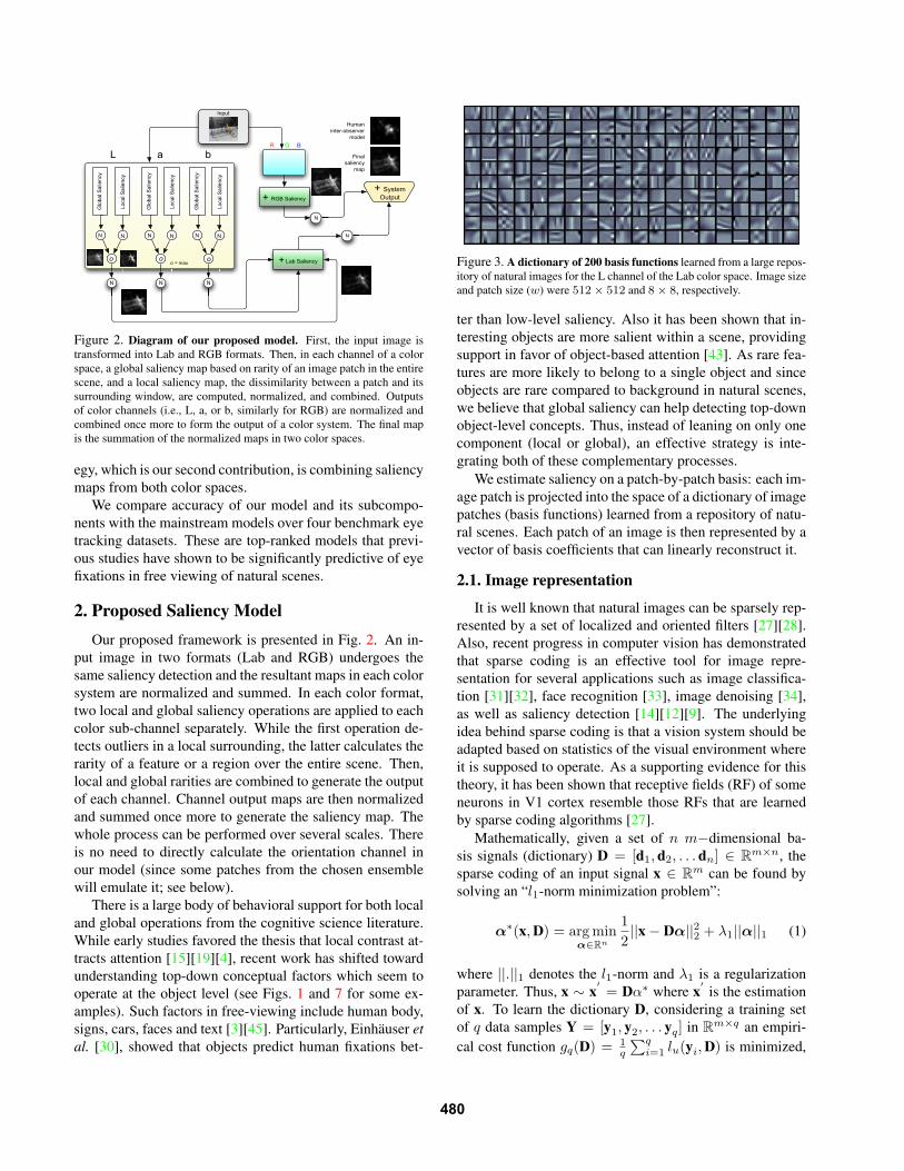
Figure 2. Diagram of our proposed model. First, the input image is
transformed into Lab and RGB formats. Then, in each channel of a color
space, a global saliency map based on rarity of an image patch in the entire
scene, and a local saliency map, the dissimilarity between a patch and its
surrounding window, are computed, normalized, and combined. Outputs
of color channels (i.e., L, a, or b, similarly for RGB) are normalized and
combined once more to form the output of a color system. The final map
is the summation of the normalized maps in two color spaces.
egy, which is our second contribution, is combining saliency
maps from both color spaces.
We compare accuracy of our model and its subcompo-
nents with the mainstream models over four benchmark eye
tracking datasets. These are top-ranked models that previ-
ous studies have shown to be significantly predictive of eye
fixations in free viewing of natural scenes.
2. Proposed Saliency ModelOur proposed framework is presented in Fig. 2. An in-
put image in two formats (Lab and RGB) undergoes the
same saliency detection and the resultant maps in each color
system are normalized and summed. In each color format,
two local and global saliency operations are applied to each
color sub-channel separately. While the first operation de-
tects outliers in a local surrounding, the latter calculates the
rarity of a feature or a region over the entire scene. Then,
local and global rarities are combined to generate the output
of each channel. Channel output maps are then normalized
and summed once more to generate the saliency map. The
whole process can be performed over several scales. There
is no need to directly calculate the orientation channel in
our model (since some patches from the chosen ensemble
will emulate it; see below).
There is a large body of behavioral support for both local
and global operations from the cognitive science literature.
While early studies favored the thesis that local contrast at-
tracts attention [15][19][4], recent work has shifted toward
understanding top-down conceptual factors which seem to
operate at the object level (see Figs. 1 and 7 for some ex-
amples). Such factors in free-viewing include human body,
signs, cars, faces and text [3][45]. Particularly, Einhauser etal. [30], showed that objects predict human fixations bet-
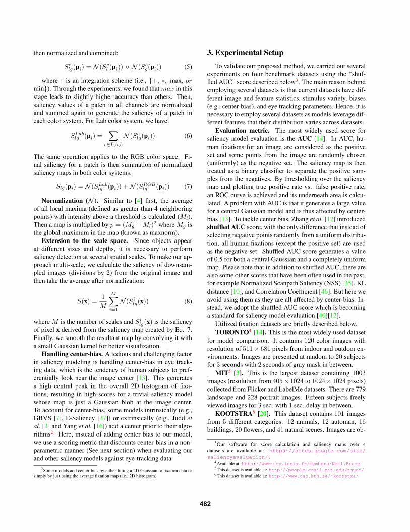
Figure 3. A dictionary of 200 basis functions learned from a large repos-
itory of natural images for the L channel of the Lab color space. Image size
and patch size (w) were 512× 512 and 8× 8, respectively.
ter than low-level saliency. Also it has been shown that in-
teresting objects are more salient within a scene, providing
support in favor of object-based attention [43]. As rare fea-
tures are more likely to belong to a single object and since
objects are rare compared to background in natural scenes,
we believe that global saliency can help detecting top-down
object-level concepts. Thus, instead of leaning on only one
component (local or global), an effective strategy is inte-
grating both of these complementary processes.
We estimate saliency on a patch-by-patch basis: each im-
age patch is projected into the space of a dictionary of image
patches (basis functions) learned from a repository of natu-
ral scenes. Each patch of an image is then represented by a
vector of basis coefficients that can linearly reconstruct it.
2.1. Image representation
It is well known that natural images can be sparsely rep-
resented by a set of localized and oriented filters [27][28].
Also, recent progress in computer vision has demonstrated
that sparse coding is an effective tool for image repre-
sentation for several applications such as image classifica-
tion [31][32], face recognition [33], image denoising [34],
as well as saliency detection [14][12][9]. The underlying
idea behind sparse coding is that a vision system should be
adapted based on statistics of the visual environment where
it is supposed to operate. As a supporting evidence for this
theory, it has been shown that receptive fields (RF) of some
neurons in V1 cortex resemble those RFs that are learned
by sparse coding algorithms [27].
Mathematically, given a set of n m−dimensional ba-
sis signals (dictionary) D = [d1, d2, . . . dn] ∈ Rm×n, the
sparse coding of an input signal x ∈ Rm can be found by
solving an “l1-norm minimization problem”:
α∗(x,D) = argminα∈Rn
1
2||x− Dα||22 + λ1||α||1 (1)
where ||.||1 denotes the l1-norm and λ1 is a regularization
parameter. Thus, x ∼ x′= Dα∗ where x
′is the estimation
of x. To learn the dictionary D, considering a training set
of q data samples Y = [y1, y2, . . . yq] in Rm×q an empiri-
cal cost function gq(D) = 1q
∑qi=1 lu(yi,D) is minimized,
480

where lu(y,D) is:
lu(yi,D) = minα∈Rn
1
2||yi − Dα||22 + λ1||α||1 (2)
We represent an image patch by a linear combination of
some basis functions which correspond or act as feature de-
tectors in early visual areas of the brain (neuron receptive
fields or transfer functions). Given an input image, it is first
resized to 2w × 2w pixels where patch size w is selected in
a way that 2w is divisible to w. Let P = {p1, p2, . . . pn}represent the set of linearized image patches from top-left
to bottom-right with no overlap. Then using Eq. 1, coef-
ficients that reconstruct each patch are calculated and are
used to represent that patch. By reshaping reconstructed
patches and aligning them, the original image can be repro-
duced.
To learn a dictionary of patch bases (i.e., minimizing
gq(D)), we extracted 500, 000 8×8 image patches (for each
sub channel of RGB or Lab) from 1500 randomly selected
color images from natural scenes. Each basis function in
the dictionary is a 8 × 8 = 64D vector. A sample learned
dictionary of size 200 is shown in Fig. 3. We experimented
with different dictionary sizes (10, 50, 100, 200, 400, and
1000) and realized that fixation prediction results did not
change much. The sparse codes αi are computed with the
above basis using the LARS algorithm [5] implemented in
the SPAMS toolbox1.
2.2. Measuring visual saliency
Our model is based on two saliency operations. The
first one, local contrast, considers the rarity of image re-
gions with respect to (small) local neighborhoods (guided
by the well-established computational architecture of Koch
and Ullman [19] and Itti et al. [4]). The second operation,
global contrast, evaluates saliency of an image patch using
its contrast with respect to the patch statistics over the entire
image. Finally, local and global contrast maps are consoli-
dated. We repeat the process for each channel of both RGB
and Lab color systems and fuse saliency maps of each sub
channel of a color space to generate a saliency map for each
color system. At each stage, maps are normalized before
integration (See Fig. 2).Local saliency. Local saliency (Sl) in our model is
the average weighted dissimilarity between a center patchi (blue rectangle in Fig. 4) and its L patches in a rectangularneighborhood (red rectangle in Fig. 4):
Scl (pi) =
1
L
L∑
j=1
W−1ij Dc
ij (3)
where Wij is the Euclidean distance between the center
patch i and the surround patch j. Thus, those patches fur-
ther away from the center patch will have less influence on
1http://www.di.ens.fr/willow/SPAMS/index.html
���� ���� ���� ��
����
����
���
��� ��� ��� ��� �� ��
���
���
��
��8
�
� ���� ���� ���� �����
����
����
���
����
���
���� ����� ���� ���� ��
����
����
����
���
...
prob
abili
ty
values for feature x
human map
distribution of each coef over the entire image
Global saliency = ∏n p(αk = ek)
Local saliency = ΣβD(α, β)
p(α2) p(αn)p(α1)
k=1
p(α3)
Figure 4. Illustration of global and local saliency for an image patch.Global saliency measures the rarity of patch in the entire scene while local
rarity measures the difference between a patch and its surrounding context.
the saliency of the center patch. Dij denotes the Euclidean
distance between patch i and patch j in the feature space be-
tween αi and αj , vectors of coefficients for patches i and j,
respectively derived from sparse coding (Sec. 2.1). While
here we use the Euclidean distance (l2 distance), the KL
distance [23][38], l1 distance [17], or correlation coefficient
have also been used in the past to calculate patch similarity.
Superscript c denotes color sub channels (L, a, or b in Labor R,G, or B in RGB).
Global saliency. It often happens that a local patch is
similar to its neighbors but the whole region (i.e., local
+ surrounding) is still in global rarity in the entire scene.
Using only the local saliency may suppress areas within a
homogeneous region resulting in blank holes, which some-
times impedes object-based attention (e.g., a uniformly tex-
tured object would only be salient at its borders). To rem-
edy such shortcoming, we build our global saliency oper-
ator guided by the information-theoretic saliency measure
of Bruce and Tsotsos [14]. Instead of each pixel, here we
calculate the probability of each patch P (pi) over the entire
scene and use its inverse as the global saliency:
Scg(pi) = P (pi)
−1 =(Πn
j=1P (αij))−1
log(Scg(pi)
)= −log(P (pi)) = −
n∑
j=1
log(P (αij))
Scg(pi) ∝ −
n∑
j=1
log(P (αij))
(4)
To calculate P (pi), we assume that coefficients α are con-
ditionally independent from each other. This is to some ex-
tent guaranteed by the sparse coding algorithm [5]. For each
coefficient of the patch representation vector (i.e., αij), first
a binned histogram (100 bins here) is calculated from all
of the patches in the scene and is then converted to a pdf
(P (αij)) by dividing to its sum. If a patch is rare in one of
the features, the above product will get a small value lead-
ing to high global saliency for that patch overall. Fig. 4
illustrates the process of calculating global saliency.
Combined saliency. Local and global saliency maps are
481
then normalized and combined:
Sclg(pi) = N (Sc
l (pi)) ◦ N (Scg(pi)) (5)
where ◦ is an integration scheme (i.e., {+, ∗, max, ormin}). Through the experiments, we found that max in this
stage leads to slightly higher accuracy than others. Then,
saliency values of a patch in all channels are normalized
and summed again to generate the saliency of a patch in
each color system. For Lab color system, we have:
SLablg (pi) =
∑
c∈L,a,b
N (Sclg(pi)) (6)
The same operation applies to the RGB color space. Fi-
nal saliency for a patch is then summation of normalized
saliency maps in both color systems:
Slg(pi) = N (SLablg (pi)) +N (SRGB
lg (pi)) (7)
Normalization (N ). Similar to [4] first, the average
of all local maxima (defined as greater than 4 neighboring
points) with intensity above a threshold is calculated (Ml).
Then a map is multiplied by p = (Mg −Ml)2 where Mg is
the global maximum in the map (known as maxnorm).
Extension to the scale space. Since objects appear
at different sizes and depths, it is necessary to perform
saliency detection at several spatial scales. To make our ap-
proach multi-scale, we calculate the saliency of downsam-
pled images (divisions by 2) from the original image and
then take the average after normalization:
S(x) =1
M
M∑
i=1
N (Silg(x)) (8)
where M is the number of scales and Silg(x) is the saliency
of pixel x derived from the saliency map created by Eq. 7.
Finally, we smooth the resultant map by convolving it with
a small Gaussian kernel for better visualization.
Handling center-bias. A tedious and challenging factor
in saliency modeling is handling center-bias in eye track-
ing data, which is the tendency of human subjects to pref-
erentially look near the image center [13]. This generates
a high central peak in the overall 2D histogram of fixa-
tions, resulting in high scores for a trivial saliency model
whose map is just a Gaussian blob at the image center.
To account for center-bias, some models intrinsically (e.g.,
GBVS [7], E-Saliency [37]) or extrinsically (e.g., Judd etal. [3] and Yang et al. [16]) add a center prior to their algo-
rithms2. Here, instead of adding center bias to our model,
we use a scoring metric that discounts center-bias in a non-
parametric manner (See next section) when evaluating our
and other saliency models against eye-tracking data.
2Some models add center-bias by either fitting a 2D Gaussian to fixation data orsimply by just using the average fixation map (i.e., 2D histogram).
3. Experimental Setup
To validate our proposed method, we carried out several
experiments on four benchmark datasets using the “shuf-
fled AUC” score described below3. The main reason behind
employing several datasets is that current datasets have dif-
ferent image and feature statistics, stimulus variety, biases
(e.g., center-bias), and eye tracking parameters. Hence, it is
necessary to employ several datasets as models leverage dif-
ferent features that their distribution varies across datasets.
Evaluation metric. The most widely used score for
saliency model evaluation is the AUC [14]. In AUC, hu-
man fixations for an image are considered as the positive
set and some points from the image are randomly chosen
(uniformly) as the negative set. The saliency map is then
treated as a binary classifier to separate the positive sam-
ples from the negatives. By thresholding over the saliency
map and plotting true positive rate vs. false positive rate,
an ROC curve is achieved and its underneath area is calcu-
lated. A problem with AUC is that it generates a large value
for a central Gaussian model and is thus affected by center-
bias [13]. To tackle center bias, Zhang et al. [12] introduced
shuffled AUC score, with the only difference that instead of
selecting negative points randomly from a uniform distribu-
tion, all human fixations (except the positive set) are used
as the negative set. Shuffled AUC score generates a value
of 0.5 for both a central Gaussian and a completely uniform
map. Please note that in addition to shuffled AUC, there are
also some other scores that have been often used in the past,
for example Normalized Scanpath Saliency (NSS) [35], KL
distance [10], and Correlation Coefficient [46]. But here we
avoid using them as they are all affected by center-bias. In-
stead, we adopt the shuffled AUC score which is becoming
a standard for saliency model evaluation [40][12].
Utilized fixation datasets are briefly described below.
TORONTO4 [14]. This is the most widely used dataset
for model comparison. It contains 120 color images with
resolution of 511× 681 pixels from indoor and outdoor en-
vironments. Images are presented at random to 20 subjects
for 3 seconds with 2 seconds of gray mask in between.
MIT5 [3]. This is the largest dataset containing 1003
images (resolution from 405× 1024 to 1024× 1024 pixels)
collected from Flicker and LabelMe datasets. There are 779
landscape and 228 portrait images. Fifteen subjects freely
viewed images for 3 sec. with 1 sec. delay in between.
KOOTSTRA6 [20]. This dataset contains 101 images
from 5 different categories: 12 animals, 12 automan, 16buildings, 20 flowers, and 41 natural scenes. Images are ob-
3Our software for score calculation and saliency maps over 4
datasets are available at: https://sites.google.com/site/saliencyevaluation/.
4Available at: http://www-sop.inria.fr/members/Neil.Bruce5This dataset is available at: http://people.csail.mit.edu/tjudd/6This dataset is available at: http://www.csc.kth.se/˜kootstra/
482

Shuf
fled
AU
C
0 0.02 0.04 0.06 0.08 0.1 0.12 0.14 0 0.02 0.04 0.06 0.08 0.1 0.12 0.14 0 0.02 0.04 0.06 0.08 0.1 0.12 0.14 0 0.02 0.04 0.06 0.08 0.1 0.12 0.14
Gaussian �
0.58
0.6
0.62
0.64
0.66
0.68
0.7
0.52
0.54
0.56
0.58
0.6
0.52
0.54
0.56
0.58
0.6
0.62
0.64
0.58
0.6
0.62
0.64
0.66
0.68AIM
GBVS
SRM
ICL
Itti
Judd
PQFT
SDSR
SUN
Surprise
Global
LG
LocalTORONTO MIT KOOTSTRA NUSEF
Figure 5. Model comparison. Fixation prediction accuracy of our saliency operations (Local, Global, LG (Local + Global)) along with 10 state-of-the-art
models over 4 benchmark datasets. X-axis indicates the σ of the Gaussian kernel (in image width) by which maps are smoothed. NUSEF dataset contains
some images with copyright which are not easily accessible and we don’t use. Only 412 images are used here.
AIM GBVS SRM ICL Itti Judd PQFT SDSR SUN Surprise Local Global LG Gauss IODataset [14] [7] [8] [9] [4] [3] [24] [11] [12] [10] Sl Sg Slg
TORONTO [14] 0.67 0.647 0.685 0.691 0.61 0.68 0.657 0.687 0.66 0.605 0.691 0.69 0.696 0.50 0.73Optimal σ 0.01 0.02 0.05 0.01 0.07 0.03 0.04 0.05 0.03 0.06 0.04 0.03 0.03 - -
MIT [3] 0.664 0.637 0.65 0.666 0.61 0.658 0.65 0.646 0.649 0.62 0.653 0.676 0.678 0.50 0.75Optimal σ 0.02 0.02 0.05 0.03 0.06 0.02 0.04 0.05 0.04 0.05 0.04 0.04 0.03 - -
KOOTSTRA [20] 0.575 0.563 0.576 0.589 0.57 0.587 0.57 0.59 0.55 0.566 0.591 0.578 0.593 0.50 0.62Optimal σ 0.01 0.01 0.04 0.01 0.07 0.02 0.03 0.03 0.02 0.07 0.03 0.02 0.03 - -
NUSEF [6] 0.623 0.595 0.62 0.614 0.56 0.61 0.60 0.60 0.60 0.58 0.583 0.627 0.632 0.49 0.66Optimal σ 0.04 0.01 0.06 0.03 0.09 0.03 0.05 0.04 0.04 0.06 0.05 0.04 0.05 - -
Table 1. Maximum performance of models shown in Fig. 5. Numbers in second rows are the sigma values where models take their maximum perfor-
mance. Parameter settings: Surround window size = 1; number of scales = 1 (256× 256). Accuracies of three best models over each dataset are shown in
bold face font. LG is the Local+Global model and IO stands for the human inter-observer model.
served by 31 subjects in the age range of 17 to 32 for 5 sec-
onds. Image resolution is 768×1024 pixels. This dataset is
specially challenging because there are not explicit objects
or salient regions within many of the images.
NUSEF7 [6]. This dataset includes 758 images contain-
ing emotionally affective scenes/objects such as expressive
faces, nudes, unpleasant concepts, and interactive actions.
In total, 75 subjects free-viewed part of the image set for 5
seconds each (on average 25 subjects per image).
4. Performance EvaluationHere, along with the evaluation of our model, we also
compare 10 state-of-the-art bottom-up saliency models.
Softwares for these models are publicly available8. Addi-
tionally, we implemented two simple models, to serve as
baseline: Gaussian Blob (Gauss) and Human inter-observer
(IO). Gaussian blob is simply a 2D Gaussian shape drawn
at the center of the image; it is expected to predict human
gaze well if such gaze is strongly clustered around the cen-
ter [13]. The human model outputs, for a given stimulus, a
map built by integrating fixations from other subjects than
the one under test while they watched that stimulus. The
human map is usually smoothed by convolving with a small
7Available at: http://mmas.comp.nus.edu.sg/NUSEF.html8 AIM: http://www-sop.inria.fr/members/Neil.Bruce/
GBVS: http://www.klab.caltech.edu/˜harel/SRM & ICL: http://www.klab.caltech.edu/˜xhou/Itti & Surprise: http://ilab.usc.edu/toolkit/Judd: http://people.csail.mit.edu/tjudd/PQFT: http://visual-attention-processing.googlecode.com/SDSR: http://alumni.soe.ucsc.edu/˜rokaf/SUN: http://cseweb.ucsd.edu/˜l6zhang/
Gaussian kernel. This model provides an upper-bound on
prediction accuracy of saliency models to the degree that,
different humans may be the best predictors of each other.
Model maps were resized to the size of the original image,
onto which eye data have been recorded.
An important parameter in model comparison is smooth-
ness (blurring) of saliency maps [40]. Here, we smoothed
the saliency map of each model by convolving it with a vari-
able size Gaussian kernel. Fig. 5 presents the shuffled AUC
score of models over the range of standard deviations σ of
the Gaussian kernel in image width (from 0.01 to 0.13 in
steps of 0.01). The maximum score value over this range
for each model is shown in Table 1. Smoothing the saliency
map dramatically affects the accuracy of some models (e.g.,
Itti, Surprise, PQFT, and SUN). Our combined saliency
model (local + global and RGB + Lab) outperforms other
models over 4 datasets with a larger margin over the MIT
and NUSEF datasets. Our local and global saliency oper-
ators have less accuracy than the combined model but are
still above several models. Results show that global saliency
works better than local saliency operator over large datasets
(MIT and NUSEF) while they are close to each other over
TORONTO dataset. Models were more successful over the
TORONTO and MIT datasets and less over KOOTSTRA
and NUSEF, possibly because of the higher complexity of
stimuli in these datasets. The NUSEF dataset contains many
affective and emotional stimuli while KOOTSTRA dataset
contains images without well-defined interesting and salient
objects (e.g., nature scenes, trees, and flowers).
483
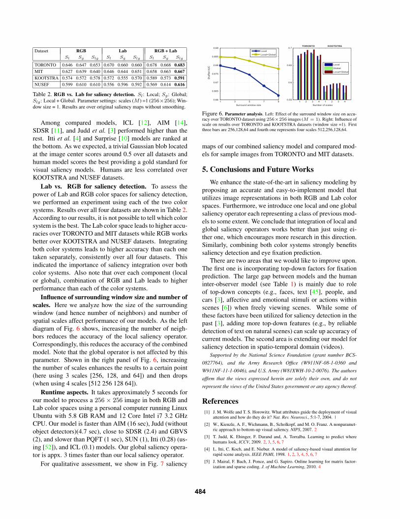
Dataset RGB Lab RGB + LabSl Sg Slg Sl Sg Slg Sl Sg Slg
TORONTO 0.646 0.647 0.653 0.670 0.660 0.660 0.678 0.668 0.683MIT 0.627 0.639 0.640 0.646 0.644 0.651 0.658 0.663 0.667KOOTSTRA 0.574 0.572 0.578 0.572 0.555 0.570 0.589 0.573 0.591NUSEF 0.599 0.610 0.610 0.556 0.596 0.592 0.569 0.614 0.616
Table 2. RGB vs. Lab for saliency detection. Sl: Local; Sg : Global;
Slg : Local + Global. Parameter settings: scales (M ) =1 (256×256); Win-
dow size = 1. Results are over original saliency maps without smoothing.
Among compared models, ICL [12], AIM [14],
SDSR [11], and Judd et al. [3] performed higher than the
rest. Itti et al. [4] and Surprise [10] models are ranked at
the bottom. As we expected, a trivial Gaussian blob located
at the image center scores around 0.5 over all datasets and
human model scores the best providing a gold standard for
visual saliency models. Humans are less correlated over
KOOTSTRA and NUSEF datasets.
Lab vs. RGB for saliency detection. To assess the
power of Lab and RGB color spaces for saliency detection,
we performed an experiment using each of the two color
systems. Results over all four datasets are shown in Table 2.
According to our results, it is not possible to tell which color
system is the best. The Lab color space leads to higher accu-
racies over TORONTO and MIT datasets while RGB works
better over KOOTSTRA and NUSEF datasets. Integrating
both color systems leads to higher accuracy than each one
taken separately, consistently over all four datasets. This
indicated the importance of saliency integration over both
color systems. Also note that over each component (local
or global), combination of RGB and Lab leads to higher
performance than each of the color systems.
Influence of surrounding window size and number ofscales. Here we analyze how the size of the surrounding
window (and hence number of neighbors) and number of
spatial scales affect performance of our models. As the left
diagram of Fig. 6 shows, increasing the number of neigh-
bors reduces the accuracy of the local saliency operator.
Correspondingly, this reduces the accuracy of the combined
model. Note that the global operator is not affected by this
parameter. Shown in the right panel of Fig. 6, increasing
the number of scales enhances the results to a certain point
(here using 3 scales [256, 128, and 64]) and then drops
(when using 4 scales [512 256 128 64]).
Runtime aspects. It takes approximately 5 seconds for
our model to process a 256 × 256 image in both RGB and
Lab color spaces using a personal computer running Linux
Ubuntu with 5.8 GB RAM and 12 Core Intel i7 3.2 GHz
CPU. Our model is faster than AIM (16 sec), Judd (without
object detectors)(4.7 sec), close to SDSR (2.4) and GBVS
(2), and slower than PQFT (1 sec), SUN (1), Itti (0.28) (us-
ing [52]), and ICL (0.1) models. Our global saliency opera-
tor is appx. 3 times faster than our local saliency operator.
For qualitative assessment, we show in Fig. 7 saliency
1 3 5 7 90.66
0.665
0.67
0.675
0.68
0.685
0.69
Shuf
fled
AUC
Surround window size Number of scales
TORONTO KOOTSTRA
1 2 3 4 1 2 3 40.55
0.6
0.65
0.7Local
Local+Global
Local
Global
Local+Global
Figure 6. Parameter analysis. Left: Effect of the surround window size on accu-racy over TORONTO dataset using 256×256 images (M = 1). Right: Influence ofscale on results over TORONTO and KOOTSTRA datasets (window size =1). Firstthree bars are 256,128,64 and fourth one represents four scales 512,256,128,64.
maps of our combined saliency model and compared mod-
els for sample images from TORONTO and MIT datasets.
5. Conclusions and Future WorksWe enhance the state-of-the-art in saliency modeling by
proposing an accurate and easy-to-implement model that
utilizes image representations in both RGB and Lab color
spaces. Furthermore, we introduce one local and one global
saliency operator each representing a class of previous mod-
els to some extent. We conclude that integration of local and
global saliency operators works better than just using ei-
ther one, which encourages more research in this direction.
Similarly, combining both color systems strongly benefits
saliency detection and eye fixation prediction.
There are two areas that we would like to improve upon.
The first one is incorporating top-down factors for fixation
prediction. The large gap between models and the human
inter-observer model (see Table 1) is mainly due to role
of top-down concepts (e.g., faces, text [45], people, and
cars [3], affective and emotional stimuli or actions within
scenes [6]) when freely viewing scenes. While some of
these factors have been utilized for saliency detection in the
past [3], adding more top-down features (e.g., by reliable
detection of text on natural scenes) can scale up accuracy of
current models. The second area is extending our model for
saliency detection in spatio-temporal domain (videos).
Supported by the National Science Foundation (grant number BCS-
0827764), and the Army Research Office (W911NF-08-1-0360 and
W911NF-11-1-0046), and U.S. Army (W81XWH-10-2-0076). The authors
affirm that the views expressed herein are solely their own, and do not
represent the views of the United States government or any agency thereof.
References[1] J. M. Wolfe and T. S. Horowitz. What attributes guide the deployment of visual
attention and how do they do it? Nat. Rev. Neurosci., 5:1-7, 2004. 1
[2] W., Kienzle, A. F., Wichmann, B., Scholkopf, and M. O. Franz. A nonparamet-ric approach to bottom-up visual saliency. NIPS, 2007. 2
[3] T. Judd, K. Ehinger, F. Durand and, A. Torralba. Learning to predict wherehumans look, ICCV, 2009. 2, 3, 5, 6, 7
[4] L. Itti, C. Koch, and E. Niebur. A model of saliency-based visual attention forrapid scene analysis. IEEE PAMI, 1998. 1, 2, 3, 4, 5, 6, 7
[5] J. Mairal, F. Bach, J. Ponce, and G. Sapiro. Online learning for matrix factor-ization and sparse coding. J. of Machine Learning, 2010. 4
484
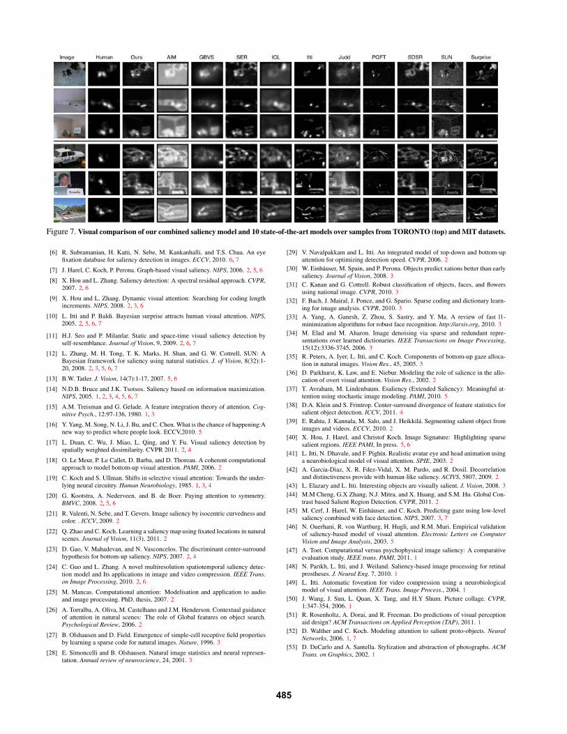
Figure 7. Visual comparison of our combined saliency model and 10 state-of-the-art models over samples from TORONTO (top) and MIT datasets.
[6] R. Subramanian, H. Katti, N. Sebe, M. Kankanhalli, and T.S. Chua. An eyefixation database for saliency detection in images. ECCV, 2010. 6, 7
[7] J. Harel, C. Koch, P. Perona. Graph-based visual saliency. NIPS, 2006. 2, 5, 6
[8] X. Hou and L. Zhang. Saliency detection: A spectral residual approach. CVPR,2007. 2, 6
[9] X. Hou and L. Zhang. Dynamic visual attention: Searching for coding lengthincrements. NIPS, 2008. 2, 3, 6
[10] L. Itti and P. Baldi. Bayesian surprise attracts human visual attention. NIPS,2005. 2, 5, 6, 7
[11] H.J. Seo and P. Milanfar. Static and space-time visual saliency detection byself-resemblance. Journal of Vision, 9, 2009. 2, 6, 7
[12] L. Zhang, M. H. Tong, T. K. Marks, H. Shan, and G. W. Cottrell, SUN: ABayesian framework for saliency using natural statistics. J. of Vision, 8(32):1-20, 2008. 2, 3, 5, 6, 7
[13] B.W. Tatler. J. Vision, 14(7):1-17, 2007. 5, 6
[14] N.D.B. Bruce and J.K. Tsotsos. Saliency based on information maximization.NIPS, 2005. 1, 2, 3, 4, 5, 6, 7
[15] A.M. Treisman and G. Gelade. A feature integration theory of attention. Cog-nitive Psych., 12:97-136, 1980. 1, 3
[16] Y. Yang, M. Song, N. Li, J. Bu, and C. Chen. What is the chance of happening:Anew way to predict where people look. ECCV,2010. 5
[17] L. Duan, C. Wu, J. Miao, L. Qing, and Y. Fu. Visual saliency detection byspatially weighted dissimilarity. CVPR 2011. 2, 4
[18] O. Le Meur, P. Le Callet, D. Barba, and D. Thoreau. A coherent computationalapproach to model bottom-up visual attention. PAMI, 2006. 2
[19] C. Koch and S. Ullman. Shifts in selective visual attention: Towards the under-lying neural circuitry. Human Neurobiology, 1985. 1, 3, 4
[20] G. Kootstra, A. Nederveen, and B. de Boer. Paying attention to symmetry.BMVC, 2008. 2, 5, 6
[21] R. Valenti, N. Sebe, and T. Gevers. Image saliency by isocentric curvedness andcolor. . ICCV, 2009. 2
[22] Q. Zhao and C. Koch. Learning a saliency map using fixated locations in naturalscenes. Journal of Vision, 11(3), 2011. 2
[23] D. Gao, V. Mahadevan, and N. Vasconcelos. The discriminant center-surroundhypothesis for bottom-up saliency. NIPS, 2007. 2, 4
[24] C. Guo and L. Zhang. A novel multiresolution spatiotemporal saliency detec-tion model and Its applications in image and video compression. IEEE Trans.on Image Processing, 2010. 2, 6
[25] M. Mancas. Computational attention: Modelisation and application to audioand image processing. PhD. thesis, 2007. 2
[26] A. Torralba, A. Oliva, M. Castelhano and J.M. Henderson. Contextual guidanceof attention in natural scenes: The role of Global features on object search.Psychological Review, 2006. 2
[27] B. Olshausen and D. Field. Emergence of simple-cell receptive field propertiesby learning a sparse code for natural images. Nature, 1996. 3
[28] E. Simoncelli and B. Olshausen. Natural image statistics and neural represen-tation. Annual review of neuroscience, 24, 2001. 3
[29] V. Navalpakkam and L. Itti. An integrated model of top-down and bottom-upattention for optimizing detection speed. CVPR, 2006. 2
[30] W. Einhauser, M. Spain, and P. Perona. Objects predict xations better than earlysaliency. Journal of Vision, 2008. 3
[31] C. Kanan and G. Cottrell. Robust classification of objects, faces, and flowersusing national image. CVPR, 2010. 3
[32] F. Bach, J. Mairal, J. Ponce, and G. Spario. Sparse coding and dictionary learn-ing for image analysis. CVPR, 2010. 3
[33] A. Yang, A. Ganesh, Z. Zhou, S. Sastry, and Y. Ma. A review of fast l1-minimization algorithms for robust face recognition. http://arxiv.org, 2010. 3
[34] M. Elad and M. Aharon. Image denoising via sparse and redundant repre-sentations over learned dictionaries. IEEE Transactions on Image Processing,15(12):3336-3745, 2006. 3
[35] R. Peters, A. Iyer, L. Itti, and C. Koch. Components of bottom-up gaze alloca-tion in natural images. Vision Res., 45, 2005. 5
[36] D. Parkhurst, K. Law, and E. Niebur. Modeling the role of salience in the allo-cation of overt visual attention. Vision Res., 2002. 2
[37] T. Avraham, M. Lindenbaum. Esaliency (Extended Saliency): Meaningful at-tention using stochastic image modeling. PAMI, 2010. 5
[38] D.A. Klein and S. Frintrop. Center-surround divergence of feature statistics forsalient object detection. ICCV, 2011. 4
[39] E. Rahtu, J. Kannala, M. Salo, and J. Heikkila. Segmenting salient object fromimages and videos. ECCV, 2010. 2
[40] X. Hou, J. Harel, and Christof Koch. Image Signature: Highlighting sparsesalient regions. IEEE PAMI, In press. 5, 6
[41] L. Itti, N. Dhavale, and F. Pighin. Realistic avatar eye and head animation usinga neurobiological model of visual attention. SPIE, 2003. 2
[42] A. Garcia-Diaz, X. R. Fdez-Vidal, X. M. Pardo, and R. Dosil. Decorrelationand distinctiveness provide with human-like saliency. ACIVS, 5807, 2009. 2
[43] L. Elazary and L. Itti. Interesting objects are visually salient. J. Vision, 2008. 3
[44] M.M Cheng, G.X Zhang, N.J. Mitra, and X. Huang, and S.M. Hu. Global Con-trast based Salient Region Detection. CVPR, 2011. 2
[45] M. Cerf, J. Harel, W. Einhauser, and C. Koch. Predicting gaze using low-levelsaliency combined with face detection. NIPS, 2007. 3, 7
[46] N. Ouerhani, R. von Wartburg, H. Hugli, and R.M. Muri. Empirical validationof saliency-based model of visual attention. Electronic Letters on ComputerVision and Image Analysis, 2003. 5
[47] A. Toet. Computational versus psychophysical image saliency: A comparativeevaluation study. IEEE trans. PAMI, 2011. 1
[48] N. Parikh, L. Itti, and J. Weiland. Saliency-based image processing for retinalprostheses. J. Neural Eng. 7, 2010. 1
[49] L. Itti. Automatic foveation for video compression using a neurobiologicalmodel of visual attention. IEEE Trans. Image Process., 2004. 1
[50] J. Wang, J. Sun, L. Quan, X. Tang, and H.Y Shum. Picture collage. CVPR,1:347-354, 2006. 1
[51] R. Rosenholtz, A. Dorai, and R. Freeman. Do predictions of visual perceptionaid design? ACM Transactions on Applied Perception (TAP), 2011. 1
[52] D. Walther and C. Koch. Modeling attention to salient proto-objects. NeuralNetworks, 2006. 1, 7
[53] D. DeCarlo and A. Santella. Stylization and abstraction of photographs. ACMTrans. on Graphics, 2002. 1
485