Exploiting a Joint Embedding Space for Generalized Zero-Shot SemanticSegmentation

Donghyeon Baek* Youngmin Oh* Bumsub Ham†

School of Electrical and Electronic Engineering, Yonsei Universityhttps://cvlab.yonsei.ac.kr/projects/JoEm

Abstract

We address the problem of generalized zero-shot se-mantic segmentation (GZS3) predicting pixel-wise seman-tic labels for seen and unseen classes. Most GZS3 meth-ods adopt a generative approach that synthesizes visualfeatures of unseen classes from corresponding semanticones (e.g., word2vec) to train novel classifiers for both seenand unseen classes. Although generative methods show de-cent performance, they have two limitations: (1) the visualfeatures are biased towards seen classes; (2) the classifiershould be retrained whenever novel unseen classes appear.We propose a discriminative approach to address these lim-itations in a unified framework. To this end, we leveragevisual and semantic encoders to learn a joint embeddingspace, where the semantic encoder transforms semantic fea-tures to semantic prototypes that act as centers for visualfeatures of corresponding classes. Specifically, we intro-duce boundary-aware regression (BAR) and semantic con-sistency (SC) losses to learn discriminative features. Ourapproach to exploiting the joint embedding space, togetherwith BAR and SC terms, alleviates the seen bias problem.At test time, we avoid the retraining process by exploitingsemantic prototypes as a nearest-neighbor (NN) classifier.To further alleviate the bias problem, we also propose an in-ference technique, dubbed Apollonius calibration (AC), thatmodulates the decision boundary of the NN classifier to theApollonius circle adaptively. Experimental results demon-strate the effectiveness of our framework, achieving a newstate of the art on standard benchmarks.

1. IntroductionRecent works using convolutional neural net-

works (CNNs) [6, 36, 45, 57] have achieved significantsuccess in semantic segmentation. They have proveneffective in various applications such as image editing [34]and autonomous driving [54], but semantic segmentation

*Equal contribution, †Corresponding author.

visualfeature

generator

newclassifier

Training

car

bicyclepersonsegmentation

network

Stage 1 Stage 2 Stage 3

car

bicycleSemantic Encoder

VisualEncoder

gradientJoint Embedding Space

person

Training Inference

decision boundary

car

bicycle

Figure 1: In contrast to generative methods [3, 32] (top), we up-date both visual and semantic encoders to learn a joint embeddingspace, and leverage a nearest neighbor classifier in the joint em-bedding space at test time (bottom). This alleviates a bias problemtowards seen classes, and avoids re-training the classifier. We visu-alize visual features and semantic prototypes by circles and stars,respectively. Best viewed in color.

in the wild still has two limitations. First, existing methodsfail to generalize to new domains/classes, assuming thattraining and test samples share the same distribution. Sec-ond, they require lots of training samples with pixel-levelground-truth labels prohibitively expensive to annotate.As a result, current methods could handle a small set ofpre-defined classes only [23].

As alternatives to pixel-level annotations, weakly-supervised semantic segmentation methods propose to ex-ploit image-level labels [19], scribbles [35], and boundingboxes [8], all of which are less labor-intensive to anno-tate. These methods, however, also require a large num-ber of weak supervisory signals to train networks for novelclasses. On the contrary, humans can easily learn to recog-nize new concepts in a scene with a few visual examples,or even with descriptions of them. Motivated by this, few-and zero-shot learning methods [29, 42, 48] have been pro-posed to recognize objects of previously unseen classes with

9536

a few annotated examples and even without them, respec-tively. For example, few-shot semantic segmentation (FS3)methods [47, 49] typically exploit an episode training strat-egy, where each episode consists of randomly sampled sup-port and query sets, to estimate query masks with a fewannotated support examples. Although these FS3 methodsshow decent performance for unseen classes, they are ca-pable of handling a single unseen class only. Recently, thework of [56] first explores the problem of zero-shot seman-tic segmentation (ZS3), where it instead exploits pre-trainedsemantic features using class names (i.e., word2vec [38]).This work, however, focuses on predicting unseen classes,even if a given image contains both seen and unseen ones.To overcome this, generalized ZS3 (GZS3) has recentlybeen introduced to consider both seen and unseen classesin a scene during inference. Motivated by generative ap-proaches [2, 50, 52] in zero-shot image classification, manyGZS3 methods [3, 15, 32] first train a segmentation net-work that consists of a feature extractor and a classifierwith seen classes. They then freeze the feature extractorto extract visual features, and discard the classifier. Withthe fixed feature extractor, a generator [14, 25] is trained toproduce visual features from semantic ones (e.g., word2vec)of corresponding classes. This enables training novel clas-sifiers with real visual features of seen classes and gener-ated ones of unseen classes (Fig. 1 top). Although genera-tive methods achieve state-of-the-art performance in GZS3,they have the following limitations: (1) the feature extractoris trained without considering semantic features, causing abias towards seen classes. The seen bias problem becomeseven worse through a multi-stage training strategy, wherethe generator and novel classifiers are trained using the fea-ture extractor; (2) the classifier needs to be re-trained when-ever a particular unseen class is newly included/excluded,hindering deployment in a practical setting, where unseenclasses are consistently emerging.

We introduce a discriminative approach for GZS3,dubbed JoEm, that addresses the limitations of generativemethods in a unified framework (Fig. 1 bottom). Specif-ically, we exploit visual and semantic encoders to learn ajoint embedding space. The semantic encoder transformssemantic features into semantic prototypes acting as centersfor visual features of corresponding classes. Our approachto using the joint embedding space avoids the multi-stagetraining, and thus alleviates the seen bias problem. To thisend, we propose to minimize the distances between visualfeatures and corresponding semantic prototypes in the jointembedding space. We have found that visual features atobject boundaries could contain a mixture of different se-mantic information due to the large receptive field of deepCNNs. Directly minimizing the distances between the vi-sual features and semantic prototypes might distract dis-criminative feature learning. To address this, we propose a

boundary-aware regression (BAR) loss that exploits seman-tic prototypes linearly interpolated to gather the visual fea-tures at object boundaries along with its efficient implemen-tation. We also propose to use a semantic consistency (SC)loss that transfers relations between seen classes from a se-mantic embedding space to the joint one, regularizing thedistances between semantic prototypes of seen classes ex-plicitly. At test time, instead of re-training the classifieras in the generative methods [3, 15, 32], our approach tolearning discriminative semantic prototypes enables using anearest neighbor (NN) classifier [7] in the joint embeddingspace. In particular, we modulate the decision boundary ofthe NN classifier using the Apollonius circle. This Apollo-nius calibration (AC) method also makes the NN classifierless susceptible to the seen bias problem. We empiricallydemonstrate the effectiveness of our framework on standardGZS3 benchmarks [10, 40], and show that AC boosts theperformance significantly. The main contributions of ourwork can be summarized as follows:

• We introduce a simple yet effective discriminative ap-proach for GZS3. We propose BAR and SC losses, whichare complementary to each other, to better learn discrim-inative representations in the joint embedding space.

• We present an effective inference technique that modu-lates the decision boundary of the NN classifier adap-tively using the Apollonius circle. This alleviates the seenbias problem significantly, even without re-training theclassifier.

• We demonstrate the effectiveness of our approach exploit-ing the joint embedding space on standard benchmarksfor GZS3 [10, 40], and show an extensive analysis withablation studies.

2. Related workZero-shot image classification. Many zero-shot learn-ing (ZSL) [11, 29, 42] methods have been proposed forimage classification. They typically rely on side informa-tion, such as attributes [11, 27], semantic features fromclass names [37, 55], or text descriptions [30, 44], for re-lating unseen and seen object classes. Early ZSL meth-ods [1, 12, 44, 55] focus on improving performance forunseen object classes, and typically adopt a discrimina-tive approach to learn a compatibility function between vi-sual and semantic embedding spaces. Among them, theworks of [13, 30, 37, 53] exploit a joint embedding spaceto better align visual and semantic features. Similarly, ourapproach leverages the joint embedding space, but differsin that (1) we tackle the task of GZS3, which is muchmore challenging than image classification, and (2) we pro-pose two complementary losses together with an effectiveinference technique, enabling learning better representa-tions and alleviating a bias towards seen classes. Note that

9537

a straightforward adaptation of discriminative ZSL meth-ods [4, 28, 41] to generalized ZSL (GZSL) suffers from theseen bias problem severely. To address this, a calibratedstacking method [5] proposes to penalize scores of seen ob-ject classes at test time. This is similar to our AC in thatboth aim at reducing the seen bias problem at test time.The calibrated stacking method, however, shifts the deci-sion boundary with a constant value, while we modulate thedecision boundary adaptively. Recently, instead of learningthe compatibility function between visual and semantic em-bedding spaces, generative methods [2, 22, 31, 46, 50, 52]attempt to address the task of GZSL by using generative ad-versarial networks [14] or variational auto-encoders [25].They first train a generator to synthesize visual featuresfrom corresponding semantic ones or attributes. The gener-ator then produces visual features of given unseen classes,and uses them to train a new classifier for both seen and un-seen classes. In this way, generative methods reformulatethe task of GZSL as a standard classification problem, out-performing the discriminative ones, especially on the gen-eralized setting.

Zero-shot semantic segmentation. Recently, there aremany attempts to extend ZSL methods for image classifica-tion to the task of semantic segmentation. They can be cat-egorized into discriminative and generative methods. Thework of [56] adopts the discriminative approach for ZS3,focusing on predicting unseen classes in a hierarchical wayusing WordNet [39]. The work of [21] argues that adverseeffects from noisy samples are significant especially in theproblem of ZS3, and proposes uncertainty-aware losses [24]to prevent a segmentation network from overfitting to them.This work, however, requires additional parameters to es-timate the uncertainty, and outputs a binary mask for agiven class only. SPNet [51] exploits a semantic embed-ding space to tackle the task of GZS3, mapping visual fea-tures to fixed semantic ones. Differently, we propose to usea joint embedding space, better aligning visual and semanticspaces, together with two complementary losses. In contrastto discriminative methods, ZS3Net [3] leverages a genera-tive moment matching network (GMMN) [33] to synthesizevisual features from corresponding semantic ones. Train-ing ZS3Net requires three stages for a segmentation net-work, the GMMN, and a new classifier, respectively. WhileZS3Net exploits semantic features of unseen classes at thelast stage only, CSRL [32] incorporates them in the secondstage, encouraging synthesized visual features to preserverelations between seen and unseen classes in the seman-tic embedding space. CaGNet [15] proposes a contextualmodule using dilated convolutional layers [43] along witha channel-wise attention mechanism [20]. This encouragesthe generator to better capture the diversity of visual fea-tures. The generative methods [3, 15, 32] share the com-mon limitations as follows: First, they require re-training

the classifier whenever novel unseen classes are incoming.Second, they rely on the multi-stage training framework,which might deteriorate the seen bias problem, with sev-eral hyperparameters (e.g., the number of synthesized vi-sual features and the number of iterations for training a newclassifier). To address these limitations, we advocate usinga discriminative approach that avoids the multi-stage train-ing scheme and re-training the classifier.

3. MethodIn this section, we concisely describe our approach to

exploiting a joint embedding space for GZS3 (Sec. 3.1), andintroduce three training losses (Sec. 3.2). We then describeour inference technique (Sec. 3.3).

3.1. OverviewFollowing the common practice in [3, 15, 32, 51], we di-

vide classes into two disjoint sets, where we denote by Sand U sets of seen and unseen classes, respectively. Wetrain our model including visual and semantic encoders withthe seen classes S only, and use the model to predict pixel-wise semantic labels of a scene for both seen and unseenclasses, S and U , at test time. To this end, we jointly updateboth encoders to learn a joint embedding space. Specifi-cally, we first extract visual features using the visual en-coder. We then input semantic features (e.g., word2vec [38])to the semantic encoder, and obtain semantic prototypesthat represent centers for visual features of correspond-ing classes. We have empirically found that visual fea-tures at object boundaries could contain a mixture of dif-ferent semantics (Fig. 2(a) middle), which causes discrep-ancies between visual features and semantic prototypes. Toaddress this, we propose to use linearly interpolated se-mantic prototypes (Fig. 2(a) bottom), and minimize thedistances between the visual features and semantic proto-types (Fig. 2(b)). We also encourage the relationships be-tween semantic prototypes to be similar to those betweensemantic features explicitly (Fig. 3). At test time, we usethe semantic prototypes of both seen and unseen classes asa NN classifier without re-training. To further reduce theseen bias problem, we modulate the decision boundary ofthe NN classifier adaptively (Fig. 4(c)). In the following,we describe our framework in detail.

3.2. TrainingWe define an overall objective for training our model

end-to-end as follows:

L = Lce + Lbar + λLsc, (1)

where we denote by Lce, Lbar, and Lsc cross-entropy (CE),BAR, and SC terms, respectively, balanced by the parame-ter λ. In the following, we describe each loss in detail.

9538

semantic features

Nearest

discrete

continuous

SemanticEncoder

SemanticEncoder

Bilinear

VisualEncoder

continuous

(a) Discrepancy between visual feature and semantic prototype maps.

Joint Embedding Space

objectboundary

semantic prototype virtual prototypevisual feature

(b) Comparison of Lcenter and Lbar.

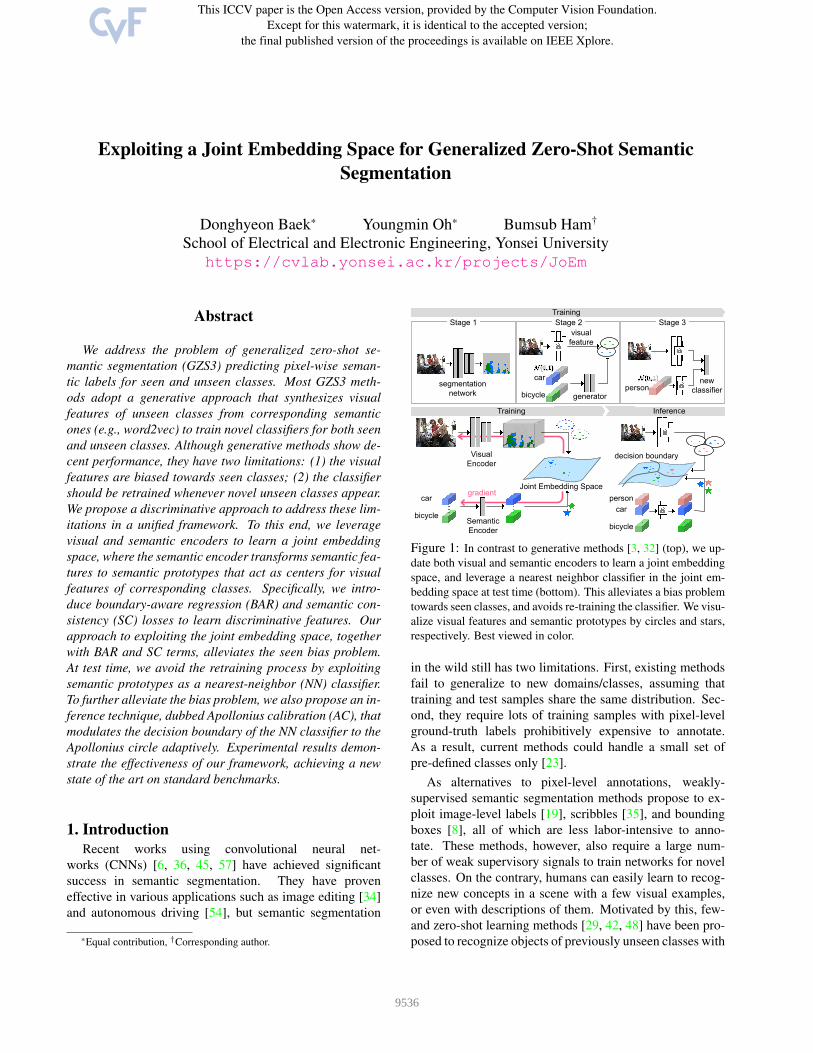
Figure 2: (a) While the semantic feature map abruptly changes at object boundaries due to the stacking operation using a ground-truthmask (top), the visual one smoothly varies due to the large receptive field of the visual encoder (middle). We leverage a series of nearest-neighbor and bilinear interpolations to smooth a sharp transition at object boundaries in an efficient way (bottom). (b) Visual features atobject boundaries might contain a mixture of different semantics, suggesting that minimizing the distances to the exact semantic prototypesis not straightforward (dashed lines). Our BAR loss exploits a virtual prototype to pull the visual features at object boundaries (solid lines).Best viewed in color.

CE loss. Given an image of size Ho × Wo, the visualencoder outputs a visual feature map v ∈ RH×W×C ,where H , W , and C are height, width, and the num-ber of channels, respectively. We denote by y a corre-sponding ground-truth mask, which is resized to the sizeof H ×W using nearest-neighbor interpolation, and v(p)a C-dimensional local visual feature at position p. Toencourage these visual features to better capture rich se-mantics specific to the task of semantic segmentation, weuse a CE loss widely adopted in supervised semantic seg-mentation. Differently, we apply this for a set of seenclasses (i.e., S) only as follows:

Lce = −1∑

c∈S |Rc|∑c∈S

∑p∈Rc

logewc·v(p)∑j∈S e

wj ·v(p), (2)

where wc is a C-dimensional classifier weight for a class cand Rc indicates a set of locations labeled as the class cin y. We denote by | · | the cardinality of a set.BAR loss. Although the CE loss trains the classifier to dis-criminate seen classes, the learned classifier weights w arenot adaptable to recognize unseen ones. To address this, weinstead use the semantic encoder as a hypernetwork [16]that generates classifier weights. Specifically, the semanticencoder transforms a semantic feature (e.g., word2vec [38])into a semantic prototype that acts as a center for visual fea-tures of a corresponding class. We then use semantic proto-types of both seen and unseen classes as a NN classifier attest time.

A straightforward way to implement this is to minimizethe distances between visual features and corresponding se-

mantic prototypes during training. To this end, we first ob-tain a semantic feature map s of sizeH×W×D as follows:

s(p) = sc for p ∈ Rc, (3)

where we denote by sc ∈ RD a semantic feature for aclass c. That is, we stack a semantic feature for a class cinto corresponding regions Rc labeled as the same class inthe ground truth y. Given the semantic feature map, the se-mantic encoder then outputs a semantic prototype map µ ofsize H ×W × C, where

µ(p) = µc for p ∈ Rc. (4)

We denote by µc ∈ RC a semantic prototype for a class c.Accordingly, we define a pixel-wise regression loss as fol-lows:

Lcenter =1∑

c∈S |Rc|∑c∈S

∑p∈Rc

d (v(p), µ(p)) , (5)

where d(·, ·) is a distance metric (e.g., Euclidean distance).This term enables learning a joint embedding space by up-dating both encoders with a gradient of Eq. (5). We haveobserved that the semantic feature map s shows a sharptransition at object boundaries due to the stacking opera-tion, making the semantic prototype map µ discrete accord-ingly1, as shown in Fig. 2(a) (top). By contrast, the vi-sual feature map v smoothly varies at object boundaries due

1This is because we use a 1 × 1 convolutional layer for the semanticencoder. Note that we could not use a CNN as the semantic encoder sinceit requires a ground-truth mask to obtain the semantic feature map at testtime.

9539

to the large receptive field of the visual encoder as shownin Fig. 2(a) (middle). That is, the visual features at ob-ject boundaries could contain a mixture of different seman-tics. Thus, directly minimizing Eq. (5) might degrade per-formance, since this could also close the distances betweensemantic prototypes as shown in Fig. 2(b) (dashed lines).To address this, we exploit linearly interpolated semanticprototypes, which we refer to as virtual prototypes. The vir-tual prototype acts as a dustbin that gathers the visual fea-tures at object boundaries as shown in Fig. 2(b) (solid lines).However, manually interpolating semantic prototypes at allboundaries could be demanding.

We introduce a simple yet effective implementation thatgives a good compromise. Specifically, we first downsam-ple the ground-truth mask y by a factor of r using nearest-neighbor interpolation. Similar to the previous case, westack semantic features but with the downsampled ground-truth mask, and obtain a semantic feature map. We up-sample this feature map by a factor of r again using bi-linear interpolation, resulting in an interpolated one s ofsize H×W ×D. Given the semantic feature map s, the se-mantic encoder outputs an interpolated semantic prototypemap µ accordingly, as shown in Fig. 2(a) (bottom). Us-ing the interpolated semantic prototype map µ, we define aBAR loss as follows:

Lbar =1∑

c∈S |Rc|∑c∈S

∑p∈Rc

d (v(p), µ(p)) . (6)

This term enables learning discriminative semantic proto-types. Note that it has been shown that uncertainty estimatesof [21] are highly activated at object boundaries. We canthus interpret the BAR loss as alleviating the influence ofvisual features at object boundaries in that this term encour-ages the visual features at object boundaries to be closer tovirtual prototypes than the exact ones. Note also that Eq. (5)is a special case of our BAR loss, that is, µ = µwhen r = 1.SC loss. Although CE and BAR terms help to learn discrim-inative representations in the joint embedding space, theydo not impose explicit constraints on the distances betweensemantic prototypes during training. To complement this,we propose to transfer the relations of semantic features inthe semantic embedding space to the semantic prototypesin the joint one. For example, we reduce the distances be-tween semantic prototypes in the joint embedding space ifcorresponding semantic features are close in the semanticone (Fig. 3). Concretely, we define the relation between twodifferent classes i and j in the semantic embedding space asfollows:

rij =e−τsd(si,sj)∑j∈S e

−τsd(si,sj), (7)

where τs is a temperature parameter that controls thesmoothness of relations. Similarly, we define the relation

Semantic Embedding Space

Joint Embedding Space

semantic prototypesemantic feature

dog

dog

person

person

cat

cat

table

table

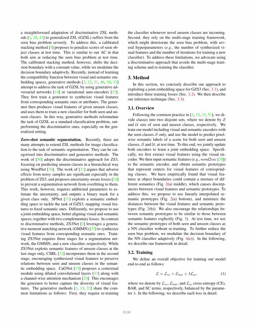
Figure 3: We visualize the relations between seen classes in se-mantic and joint embedding spaces. Our SC loss transfers the re-lations from the semantic embedding space to the joint one. Thisadjusts the distances between semantic prototypes explicitly, com-plementing the BAR loss. Best viewed in color.

in the joint embedding space as follows:

rij =e−τµd(µi,µj)∑j∈S e

−τµd(µi,µj), (8)

where τµ is a temperature parameter. To encourage the con-sistency between two embedding spaces, we define a SCloss as follows:

Lsc = −∑i∈S

∑j∈S

rij logrijrij. (9)

This term regularizes the distances between semantic pro-totypes of seen classes. Similarly, CSRL [32] distills therelations of real visual features to the synthesized ones. Ithowever exploits semantic features of unseen classes dur-ing training, suggesting that both generator and classifiershould be trained again to handle novel unseen classes.

3.3. InferenceOur discriminative approach enables handling semantic

features of arbitrary classes at test time without re-training,which is suitable for real-world scenarios. Specifically, thesemantic encoder takes semantic features of both seen andunseen classes, and outputs corresponding semantic proto-types. We then compute the distances from individual visualfeatures to each semantic prototype. That is, we formulatethe inference process as a retrieval task using the semanticprototypes as a NN classifier in the joint embedding space.A straightforward way to classify each visual feature2 is toassign the class of its nearest semantic prototype as follows:

ynn(p) = argminc∈S∪U

d(v(p), µc). (10)

Although our approach learns discriminative visual fea-tures and semantic prototypes, visual features of un-seen classes might still be biased towards those of seenclasses (Fig. 4(a)), especially when both have similar ap-pearance. For example, a cat (a unseen object class) is more

2We upsample v into the image resolution Ho × Wo using bilinearinterpolation for inference.

9540

seen unseen seen unseen

(a) Visualization of a seen bias problem.

(b) CS [5].

(c) AC.

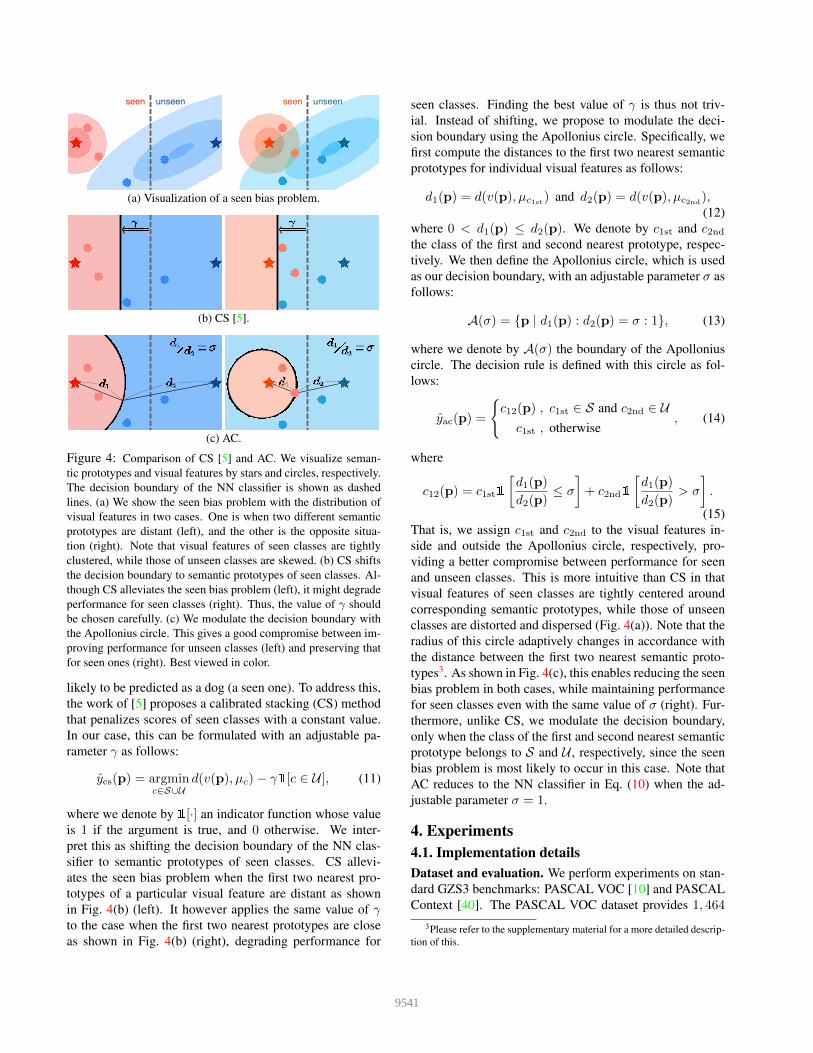
Figure 4: Comparison of CS [5] and AC. We visualize seman-tic prototypes and visual features by stars and circles, respectively.The decision boundary of the NN classifier is shown as dashedlines. (a) We show the seen bias problem with the distribution ofvisual features in two cases. One is when two different semanticprototypes are distant (left), and the other is the opposite situa-tion (right). Note that visual features of seen classes are tightlyclustered, while those of unseen classes are skewed. (b) CS shiftsthe decision boundary to semantic prototypes of seen classes. Al-though CS alleviates the seen bias problem (left), it might degradeperformance for seen classes (right). Thus, the value of γ shouldbe chosen carefully. (c) We modulate the decision boundary withthe Apollonius circle. This gives a good compromise between im-proving performance for unseen classes (left) and preserving thatfor seen ones (right). Best viewed in color.

likely to be predicted as a dog (a seen one). To address this,the work of [5] proposes a calibrated stacking (CS) methodthat penalizes scores of seen classes with a constant value.In our case, this can be formulated with an adjustable pa-rameter γ as follows:

ycs(p) = argminc∈S∪U

d(v(p), µc)− γ1[c ∈ U ], (11)

where we denote by 1[·] an indicator function whose valueis 1 if the argument is true, and 0 otherwise. We inter-pret this as shifting the decision boundary of the NN clas-sifier to semantic prototypes of seen classes. CS allevi-ates the seen bias problem when the first two nearest pro-totypes of a particular visual feature are distant as shownin Fig. 4(b) (left). It however applies the same value of γto the case when the first two nearest prototypes are closeas shown in Fig. 4(b) (right), degrading performance for

seen classes. Finding the best value of γ is thus not triv-ial. Instead of shifting, we propose to modulate the deci-sion boundary using the Apollonius circle. Specifically, wefirst compute the distances to the first two nearest semanticprototypes for individual visual features as follows:

d1(p) = d(v(p), µc1st) and d2(p) = d(v(p), µc2nd),(12)

where 0 < d1(p) ≤ d2(p). We denote by c1st and c2ndthe class of the first and second nearest prototype, respec-tively. We then define the Apollonius circle, which is usedas our decision boundary, with an adjustable parameter σ asfollows:

A(σ) = {p | d1(p) : d2(p) = σ : 1}, (13)

where we denote by A(σ) the boundary of the Apolloniuscircle. The decision rule is defined with this circle as fol-lows:

yac(p) =

{c12(p) , c1st ∈ S and c2nd ∈ Uc1st , otherwise

, (14)

where

c12(p) = c1st1

[d1(p)

d2(p)≤ σ

]+ c2nd1

[d1(p)

d2(p)> σ

].

(15)That is, we assign c1st and c2nd to the visual features in-side and outside the Apollonius circle, respectively, pro-viding a better compromise between performance for seenand unseen classes. This is more intuitive than CS in thatvisual features of seen classes are tightly centered aroundcorresponding semantic prototypes, while those of unseenclasses are distorted and dispersed (Fig. 4(a)). Note that theradius of this circle adaptively changes in accordance withthe distance between the first two nearest semantic proto-types3. As shown in Fig. 4(c), this enables reducing the seenbias problem in both cases, while maintaining performancefor seen classes even with the same value of σ (right). Fur-thermore, unlike CS, we modulate the decision boundary,only when the class of the first and second nearest semanticprototype belongs to S and U , respectively, since the seenbias problem is most likely to occur in this case. Note thatAC reduces to the NN classifier in Eq. (10) when the ad-justable parameter σ = 1.

4. Experiments4.1. Implementation detailsDataset and evaluation. We perform experiments on stan-dard GZS3 benchmarks: PASCAL VOC [10] and PASCALContext [40]. The PASCAL VOC dataset provides 1, 464

3Please refer to the supplementary material for a more detailed descrip-tion of this.

9541

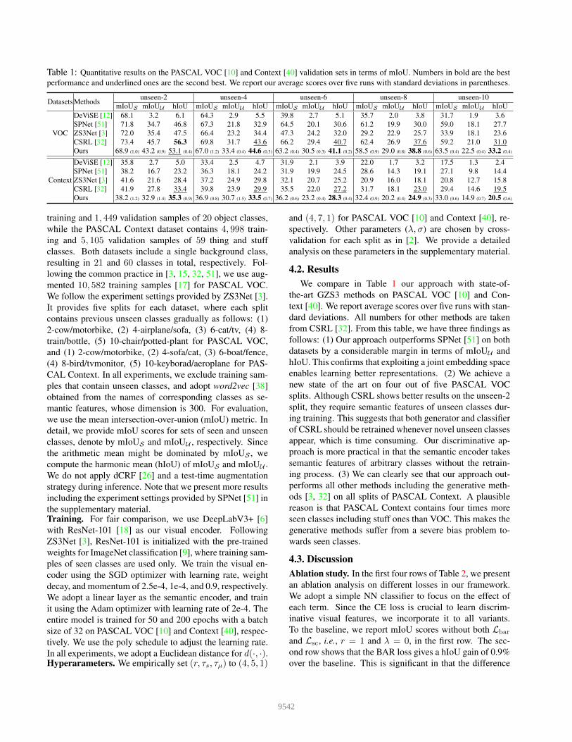
Table 1: Quantitative results on the PASCAL VOC [10] and Context [40] validation sets in terms of mIoU. Numbers in bold are the bestperformance and underlined ones are the second best. We report our average scores over five runs with standard deviations in parentheses.

Datasets Methods unseen-2 unseen-4 unseen-6 unseen-8 unseen-10mIoUS mIoUU hIoU mIoUS mIoUU hIoU mIoUS mIoUU hIoU mIoUS mIoUU hIoU mIoUS mIoUU hIoU

VOC

DeViSE [12] 68.1 3.2 6.1 64.3 2.9 5.5 39.8 2.7 5.1 35.7 2.0 3.8 31.7 1.9 3.6SPNet [51] 71.8 34.7 46.8 67.3 21.8 32.9 64.5 20.1 30.6 61.2 19.9 30.0 59.0 18.1 27.7ZS3Net [3] 72.0 35.4 47.5 66.4 23.2 34.4 47.3 24.2 32.0 29.2 22.9 25.7 33.9 18.1 23.6CSRL [32] 73.4 45.7 56.3 69.8 31.7 43.6 66.2 29.4 40.7 62.4 26.9 37.6 59.2 21.0 31.0Ours 68.9 (1.0) 43.2 (0.9) 53.1 (0.4) 67.0 (1.2) 33.4 (0.4) 44.6 (0.3) 63.2 (0.4) 30.5 (0.3) 41.1 (0.2) 58.5 (0.9) 29.0 (0.8) 38.8 (0.6) 63.5 (0.4) 22.5 (0.4) 33.2 (0.4)

Context

DeViSE [12] 35.8 2.7 5.0 33.4 2.5 4.7 31.9 2.1 3.9 22.0 1.7 3.2 17.5 1.3 2.4SPNet [51] 38.2 16.7 23.2 36.3 18.1 24.2 31.9 19.9 24.5 28.6 14.3 19.1 27.1 9.8 14.4ZS3Net [3] 41.6 21.6 28.4 37.2 24.9 29.8 32.1 20.7 25.2 20.9 16.0 18.1 20.8 12.7 15.8CSRL [32] 41.9 27.8 33.4 39.8 23.9 29.9 35.5 22.0 27.2 31.7 18.1 23.0 29.4 14.6 19.5Ours 38.2 (1.2) 32.9 (1.4) 35.3 (0.9) 36.9 (0.8) 30.7 (1.5) 33.5 (0.7) 36.2 (0.6) 23.2 (0.4) 28.3 (0.4) 32.4 (0.9) 20.2 (0.4) 24.9 (0.3) 33.0 (0.6) 14.9 (0.7) 20.5 (0.6)

training and 1, 449 validation samples of 20 object classes,while the PASCAL Context dataset contains 4, 998 train-ing and 5, 105 validation samples of 59 thing and stuffclasses. Both datasets include a single background class,resulting in 21 and 60 classes in total, respectively. Fol-lowing the common practice in [3, 15, 32, 51], we use aug-mented 10, 582 training samples [17] for PASCAL VOC.We follow the experiment settings provided by ZS3Net [3].It provides five splits for each dataset, where each splitcontains previous unseen classes gradually as follows: (1)2-cow/motorbike, (2) 4-airplane/sofa, (3) 6-cat/tv, (4) 8-train/bottle, (5) 10-chair/potted-plant for PASCAL VOC,and (1) 2-cow/motorbike, (2) 4-sofa/cat, (3) 6-boat/fence,(4) 8-bird/tvmonitor, (5) 10-keyborad/aeroplane for PAS-CAL Context. In all experiments, we exclude training sam-ples that contain unseen classes, and adopt word2vec [38]obtained from the names of corresponding classes as se-mantic features, whose dimension is 300. For evaluation,we use the mean intersection-over-union (mIoU) metric. Indetail, we provide mIoU scores for sets of seen and unseenclasses, denote by mIoUS and mIoUU , respectively. Sincethe arithmetic mean might be dominated by mIoUS , wecompute the harmonic mean (hIoU) of mIoUS and mIoUU .We do not apply dCRF [26] and a test-time augmentationstrategy during inference. Note that we present more resultsincluding the experiment settings provided by SPNet [51] inthe supplementary material.Training. For fair comparison, we use DeepLabV3+ [6]with ResNet-101 [18] as our visual encoder. FollowingZS3Net [3], ResNet-101 is initialized with the pre-trainedweights for ImageNet classification [9], where training sam-ples of seen classes are used only. We train the visual en-coder using the SGD optimizer with learning rate, weightdecay, and momentum of 2.5e-4, 1e-4, and 0.9, respectively.We adopt a linear layer as the semantic encoder, and trainit using the Adam optimizer with learning rate of 2e-4. Theentire model is trained for 50 and 200 epochs with a batchsize of 32 on PASCAL VOC [10] and Context [40], respec-tively. We use the poly schedule to adjust the learning rate.In all experiments, we adopt a Euclidean distance for d(·, ·).Hyperarameters. We empirically set (r, τs, τµ) to (4, 5, 1)

and (4, 7, 1) for PASCAL VOC [10] and Context [40], re-spectively. Other parameters (λ, σ) are chosen by cross-validation for each split as in [2]. We provide a detailedanalysis on these parameters in the supplementary material.

4.2. ResultsWe compare in Table 1 our approach with state-of-

the-art GZS3 methods on PASCAL VOC [10] and Con-text [40]. We report average scores over five runs with stan-dard deviations. All numbers for other methods are takenfrom CSRL [32]. From this table, we have three findings asfollows: (1) Our approach outperforms SPNet [51] on bothdatasets by a considerable margin in terms of mIoUU andhIoU. This confirms that exploiting a joint embedding spaceenables learning better representations. (2) We achieve anew state of the art on four out of five PASCAL VOCsplits. Although CSRL shows better results on the unseen-2split, they require semantic features of unseen classes dur-ing training. This suggests that both generator and classifierof CSRL should be retrained whenever novel unseen classesappear, which is time consuming. Our discriminative ap-proach is more practical in that the semantic encoder takessemantic features of arbitrary classes without the retrain-ing process. (3) We can clearly see that our approach out-performs all other methods including the generative meth-ods [3, 32] on all splits of PASCAL Context. A plausiblereason is that PASCAL Context contains four times moreseen classes including stuff ones than VOC. This makes thegenerative methods suffer from a severe bias problem to-wards seen classes.

4.3. DiscussionAblation study. In the first four rows of Table 2, we presentan ablation analysis on different losses in our framework.We adopt a simple NN classifier to focus on the effect ofeach term. Since the CE loss is crucial to learn discrim-inative visual features, we incorporate it to all variants.To the baseline, we report mIoU scores without both Lbar

and Lsc, i.e., r = 1 and λ = 0, in the first row. The sec-ond row shows that the BAR loss gives a hIoU gain of 0.9%over the baseline. This is significant in that the difference

9542

between the first two rows is whether a series of two inter-polations is applied to a semantic feature map or not, be-fore inputting it to a semantic encoder (see Sec. 3.2). Wecan also see that explicitly regularizing the distances be-tween semantic prototypes improves performance for un-seen classes in the third row. The fourth row demonstratesthat BAR and SC terms are complementary to each other,achieving the best performance.

Comparison with CS. The last two rows in Table 2 show aquantitative comparison of CS [5] and AC in terms of mIoUscores. We can see that both CS and AC improve perfor-mance for unseen classes by large margins. A reason is thatvisual features for unseen classes are skewed and biased to-wards those of seen classes (Fig. 4(a)). It is worth notingthat AC further achieves a mIoUU gain of 2.7% over CSwith a negligible overhead, demonstrating the effectivenessof using the Apollonius circle. In Fig. 5, we plot perfor-mance variations according to the adjustable parameter foreach method, i.e., γ and σ, in the range of [0, 12] and (0, 1]with intervals of 0.5 and 0.05 for CS and AC, respectively.We first compare the mIoUU -mIoUS curves in Fig. 5 (left).For comparison, we visualize the mIoUS of the NN clas-sifier by a dashed line. We can see that AC always givesbetter mIoUU scores for all mIoUS values on the left-handside of the dashed line, suggesting that AC is more robustw.r.t. the adjustable parameter. We also show that how falsenegatives of seen classes change according to true positivesof unseen classes (TPU ) in Fig. 5 (right). In particular, wecompute false negatives of seen classes, when they are pre-dicted as one of unseen classes, denoted by FNS→U . Wecan clearly see that CS has more FNS→U than AC at thesame value of TPU , confirming once again that AC is morerobust to the parameter, while providing better results.

Analysis of embedding spaces. To verify that exploit-ing a joint embedding space alleviates a seen bias prob-lem, we compare in Table 3 variants of our approach withZS3Net [3]. First, we attempt to project visual features tocorresponding semantic ones without exploiting a semanticencoder. This, however, provides a trivial solution that allvisual features are predicted as a background class. Second,we adopt a two-stage discriminative approach, that is, train-ing visual and semantic encoders sequentially. We first traina segmentation network that consists of a feature extractorand a classifier with seen classes. The learned feature ex-tractor is then fixed and it is used as a visual encoder totrain a semantic encoder (‘S→V’). We can see from the firsttwo rows that this simple variant with BAR and SC termsalready outperforms ZS3Net, demonstrating the effective-ness of the discriminative approach. These variants are,however, outperformed by our approach that gives the besthIoU score of 44.6 (Table 1). To further verify our claim,we train the generator of ZS3Net using visual features ex-tracted from our visual encoder (‘ZS3Net‡’). For compar-

Table 2: Comparison of mIoU scores using different loss termsand inference techniques on the unseen-4 split of PASCAL Con-text [40]. For an ablation study on different loss terms, we use aNN classifier without applying any inference techniques in orderto focus more on the effect of each term. CS: calibrated stack-ing [5]; AC: Apollonius circle.

Lce Lcenter Lbar Lsc CS AC mIoUS mIoUU hIoUX X 37.7 10.0 15.8X X 37.9 10.7 16.7X X X 36.1 11.8 17.8X X X 36.2 12.9 19.0X X X X 36.2 29.1 32.3X X X X 35.7 31.8 33.7

32 34 36mIoUS

15

20

25

30

mIo

UU

NN

ACCS

2.0 2.5 3.0 3.5 4.0TPU (×107)

1

2

3

4

FNS→U (×

107) AC

CS

Figure 5: Comparison of CS [5] and AC by varying γ and σ,respectively, on the unseen-4 split of PASCAL Context [40]. Weshow the mIoUU -mIoUS curves (left), and how FNS→U changesw.r.t. TPU (right). Best viewed in color.

Table 3: Quantitative comparison on the unseen-4 split of PAS-CAL VOC [10]. †: reimplementation; ‡: our visual encoder.

Methods mIoUS mIoUU hIoUS→V: Lcenter 61.7 20.9 31.2S→V: Lbar + Lsc 65.7 30.3 41.5ZS3Net [3] 66.4 23.2 34.4ZS3Net† 68.8 28.8 40.6ZS3Net‡ 68.5 31.8 43.4

ison, we also report the results obtained by our implemen-tation of ZS3Net (‘ZS3Net†’). From the last two rows, wecan clearly see that ‘ZS3Net‡’ outperforms ‘ZS3Net†’. Thisconfirms that our approach alleviates the seen bias problem,enhancing the generalization ability of visual features.

5. ConclusionWe have introduced a discriminative approach, dubbed

JoEm, that overcomes the limitations of generative ones ina unified framework. We have proposed two complemen-tary losses to better learn representations in a joint embed-ding space. We have also presented a novel inference tech-nique using the circle of Apollonius that alleviates a seenbias problem significantly. Finally, we have shown that ourapproach achieves a new state of the art on standard GZS3benchmarks.Acknowledgments. This work was supported in partby the National Research Foundation of Korea (NRF)grant funded by the Korea government (MSIP) (NRF-2019R1A2C2084816) and the Yonsei University ResearchFund of 2021 (2021-22-0001).

9543

References[1] Zeynep Akata, Scott Reed, Daniel Walter, Honglak Lee, and

Bernt Schiele. Evaluation of output embeddings for fine-grained image classification. In CVPR, 2015. 2

[2] Maxime Bucher, Stephane Herbin, and Frederic Jurie. Gen-erating visual representations for zero-shot classification. InICCV Workshops, 2017. 2, 3, 7

[3] Maxime Bucher, VU Tuan-Hung, Matthieu Cord, andPatrick Perez. Zero-shot semantic segmentation. In NeurIPS,2019. 1, 2, 3, 7, 8

[4] Soravit Changpinyo, Wei-Lun Chao, Boqing Gong, and FeiSha. Synthesized classifiers for zero-shot learning. In CVPR,2016. 3

[5] Wei-Lun Chao, Soravit Changpinyo, Boqing Gong, and FeiSha. An empirical study and analysis of generalized zero-shot learning for object recognition in the wild. In ECCV,2016. 3, 6, 8

[6] Liang-Chieh Chen, Yukun Zhu, George Papandreou, FlorianSchroff, and Hartwig Adam. Encoder-decoder with atrousseparable convolution for semantic image segmentation. InECCV, 2018. 1, 7

[7] Thomas Cover and Peter Hart. Nearest neighbor pattern clas-sification. IEEE Trans. Information Theory, 13(1):21–27,1967. 2

[8] Jifeng Dai, Kaiming He, and Jian Sun. BoxSup: Exploit-ing bounding boxes to supervise convolutional networks forsemantic segmentation. In ICCV, 2015. 1

[9] Jia Deng, Wei Dong, Richard Socher, Li-Jia Li, Kai Li,and Li Fei-Fei. ImageNet: A large-scale hierarchical imagedatabase. In CVPR, 2009. 7

[10] Mark Everingham, Luc Van Gool, Christopher KI Williams,John Winn, and Andrew Zisserman. The pascal visual objectclasses (VOC) challenge. IJCV, 88(2):303–338, 2010. 2, 6,7, 8

[11] Ali Farhadi, Ian Endres, Derek Hoiem, and David Forsyth.Describing objects by their attributes. In CVPR, 2009. 2

[12] Andrea Frome, Greg Corrado, Jonathon Shlens, SamyBengio, Jeffrey Dean, Marc’Aurelio Ranzato, and TomasMikolov. DeViSE: A deep visual-semantic embeddingmodel. In NeurIPS, 2013. 2, 7

[13] Yanwei Fu, Timothy M Hospedales, Tao Xiang, ZhenyongFu, and Shaogang Gong. Transductive multi-view embed-ding for zero-shot recognition and annotation. In ECCV,2014. 2

[14] Ian J Goodfellow, Jean Pouget-Abadie, Mehdi Mirza, BingXu, David Warde-Farley, Sherjil Ozair, Aaron Courville,and Yoshua Bengio. Generative adversarial networks. InNeurIPS, 2014. 2, 3

[15] Zhangxuan Gu, Siyuan Zhou, Li Niu, Zihan Zhao, andLiqing Zhang. Context-aware feature generation for zero-shot semantic segmentation. In ACM MM, 2020. 2, 3, 7

[16] David Ha, Andrew Dai, and Quoc V Le. Hypernetworks. InICLR, 2017. 4

[17] Bharath Hariharan, Pablo Arbelaez, Lubomir Bourdev,Subhransu Maji, and Jitendra Malik. Semantic contours frominverse detectors. In ICCV, 2011. 7

[18] Kaiming He, Xiangyu Zhang, Shaoqing Ren, and Jian Sun.Deep residual learning for image recognition. In CVPR,2016. 7

[19] Qibin Hou, Peng-Tao Jiang, Yunchao Wei, and Ming-MingCheng. Self-erasing network for integral object attention. InNeurIPS, 2018. 1

[20] Jie Hu, Li Shen, and Gang Sun. Squeeze-and-excitation net-works. In CVPR, 2018. 3

[21] Ping Hu, Stan Sclaroff, and Kate Saenko. Uncertainty-awarelearning for zero-shot semantic segmentation. In NeurIPS,2020. 3, 5

[22] He Huang, Changhu Wang, Philip S Yu, and Chang-DongWang. Generative dual adversarial network for generalizedzero-shot learning. In CVPR, 2019. 3

[23] Shipra Jain, Danda Paudel Pani, Martin Danelljan, and LucVan Gool. Scaling semantic segmentation beyond 1K classeson a single GPU. arXiv preprint arXiv:2012.07489, 2020. 1

[24] Alex Kendall and Yarin Gal. What uncertainties do we needin bayesian deep learning for computer vision? In NeurIPS,2017. 3

[25] Diederik P Kingma and Max Welling. Auto-encoding varia-tional bayes. In ICLR, 2014. 2, 3

[26] Philipp Krahenbuhl and Vladlen Koltun. Efficient inferencein fully connected CRFs with gaussian edge potentials. InNeurIPS, 2011. 7

[27] Christoph H Lampert, Hannes Nickisch, and Stefan Harmel-ing. Learning to detect unseen object classes by between-class attribute transfer. In CVPR, 2009. 2

[28] Christoph H Lampert, Hannes Nickisch, and Stefan Harmel-ing. Attribute-based classification for zero-shot visual objectcategorization. IEEE Trans. PAMI, 36(3):453–465, 2013. 3

[29] Hugo Larochelle, Dumitru Erhan, and Yoshua Bengio. Zero-data learning of new tasks. In AAAI, 2008. 1, 2

[30] Jimmy Lei Ba, Kevin Swersky, Sanja Fidler, et al. Predictingdeep zero-shot convolutional neural networks using textualdescriptions. In ICCV, 2015. 2

[31] Jingjing Li, Mengmeng Jing, Ke Lu, Zhengming Ding, LeiZhu, and Zi Huang. Leveraging the invariant side of genera-tive zero-shot learning. In CVPR, 2019. 3

[32] Peike Li, Yunchao Wei, and Yi Yang. Consistent structuralrelation learning for zero-shot segmentation. In NeurIPS,2020. 1, 2, 3, 5, 7

[33] Yujia Li, Kevin Swersky, and Rich Zemel. Generative mo-ment matching networks. In ICML, 2015. 3

[34] Xiaodan Liang, Hao Zhang, Liang Lin, and Eric Xing. Gen-erative semantic manipulation with mask-contrasting gan. InECCV, 2018. 1

[35] Di Lin, Jifeng Dai, Jiaya Jia, Kaiming He, and Jian Sun.ScribbleSup: Scribble-supervised convolutional networksfor semantic segmentation. In CVPR, 2016. 1

[36] Jonathan Long, Evan Shelhamer, and Trevor Darrell. Fullyconvolutional networks for semantic segmentation. InCVPR, 2015. 1

[37] Yao Lu. Unsupervised learning on neural network outputs:with application in zero-shot learning. In IJCAI, 2016. 2

[38] Tomas Mikolov, Ilya Sutskever, Kai Chen, Greg Corrado,and Jeffrey Dean. Distributed representations of words and

9544

phrases and their compositionality. In NeurIPS, 2013. 2, 3,4, 7

[39] George A Miller. WordNet: A lexical database for english.Communications of the ACM, 38(11):39–41, 1995. 3

[40] Roozbeh Mottaghi, Xianjie Chen, Xiaobai Liu, Nam-GyuCho, Seong-Whan Lee, Sanja Fidler, Raquel Urtasun, andAlan Yuille. The role of context for object detection and se-mantic segmentation in the wild. In CVPR, 2014. 2, 6, 7,8

[41] Mohammad Norouzi, Tomas Mikolov, Samy Bengio, YoramSinger, Jonathon Shlens, Andrea Frome, Greg S Corrado,and Jeffrey Dean. Zero-shot learning by convex combinationof semantic embeddings. In ICLR, 2014. 3

[42] Mark M Palatucci, Dean A Pomerleau, Geoffrey E Hinton,and Tom Mitchell. Zero-shot learning with semantic outputcodes. In NeurIPS, 2009. 1, 2

[43] George Papandreou, Iasonas Kokkinos, and Pierre-AndreSavalle. Untangling local and global deformations in deepconvolutional networks for image classification and slidingwindow detection. arXiv preprint arXiv:1412.0296, 2014. 3

[44] Scott Reed, Zeynep Akata, Honglak Lee, and Bernt Schiele.Learning deep representations of fine-grained visual descrip-tions. In CVPR, 2016. 2

[45] Olaf Ronneberger, Philipp Fischer, and Thomas Brox. U-Net: Convolutional networks for biomedical image segmen-tation. In MICCAI, 2015. 1

[46] Mert Bulent Sariyildiz and Ramazan Gokberk Cinbis. Gradi-ent matching generative networks for zero-shot learning. InCVPR, 2019. 3

[47] Amirreza Shaban, Shray Bansal, Zhen Liu, Irfan Essa, andByron Boots. One-shot learning for semantic segmentation.In BMVC, 2017. 2

[48] Oriol Vinyals, Charles Blundell, Timothy Lillicrap, KorayKavukcuoglu, and Daan Wierstra. Matching networks forone shot learning. In NeurIPS, 2016. 1

[49] Kaixin Wang, Jun Hao Liew, Yingtian Zou, Daquan Zhou,and Jiashi Feng. PANet: Few-shot image semantic segmen-tation with prototype alignment. In ICCV, 2019. 2

[50] Wenlin Wang, Yunchen Pu, Vinay Verma, Kai Fan, YizheZhang, Changyou Chen, Piyush Rai, and Lawrence Carin.Zero-shot learning via class-conditioned deep generativemodels. In AAAI, 2018. 2, 3

[51] Yongqin Xian, Subhabrata Choudhury, Yang He, BerntSchiele, and Zeynep Akata. Semantic projection network forzero-and few-label semantic segmentation. In CVPR, 2019.3, 7

[52] Yongqin Xian, Tobias Lorenz, Bernt Schiele, and ZeynepAkata. Feature generating networks for zero-shot learning.In CVPR, 2018. 2, 3

[53] Yongxin Yang and Timothy M Hospedales. A unified per-spective on multi-domain and multi-task learning. In ICLR,2015. 2

[54] Ekim Yurtsever, Jacob Lambert, Alexander Carballo, andKazuya Takeda. A survey of autonomous driving: Com-mon practices and emerging technologies. IEEE Access,8:58443–58469, 2020. 1

[55] Li Zhang, Tao Xiang, and Shaogang Gong. Learning a deepembedding model for zero-shot learning. In CVPR, 2017. 2

[56] Hang Zhao, Xavier Puig, Bolei Zhou, Sanja Fidler, and An-tonio Torralba. Open vocabulary scene parsing. In ICCV,2017. 2, 3

[57] Hengshuang Zhao, Jianping Shi, Xiaojuan Qi, XiaogangWang, and Jiaya Jia. Pyramid scene parsing network. InCVPR, 2017. 1

9545