Explicit Ion, Implicit Water Solvation for Molecular ...crystal.med.upenn.edu/sharp-lab-pdfs/prabhu_zapdna_Jcompchem_2… · Explicit Ion, Implicit Water Solvation for Molecular Dynamics

Explicit Ion, Implicit Water Solvation for Molecular

Dynamics of Nucleic Acids and Highly Charged Molecules

NINAD V. PRABHU,1 MANORANJAN PANDA,2 QINGYI YANG,3 KIM A. SHARP3

1Schering-Plough, Kenilworth, NJ, USA2Astra-Zeneca, Bangalore, India

3Department of Biochemistry and Biophysics, Johnson Research Foundation,University of Pennsylvania, Philadelphia, Pennsylvania 19104

Received 15 June 2007; Revised 21 September 2007; Accepted 12 October 2007DOI 10.1002/jcc.20874

Published online 11 December 2007 in Wiley InterScience (www.interscience.wiley.com).

Abstract: An explicit ion, implicit water solvent model for molecular dynamics was developed and tested with

DNA and RNA simulations. The implicit water model uses the finite difference Poisson (FDP) model with the

smooth permittivity method implemented in the OpenEye ZAP libraries. Explicit counter-ions, co-ions, and nucleic

acid were treated with a Langevin dynamics molecular dynamics algorithm. Ion electrostatics is treated within the

FDP model when close to the solute, and by the Coulombic model when far from the solute. The two zone model

reduces computation time, but retains an accurate treatment of the ion atmosphere electrostatics near the solute. Ion

compositions can be set to reproduce specific ionic strengths. The entire ion/water treatment is interfaced with the

molecular dynamics package CHARMM. Using the CHARMM-ZAPI software combination, the implicit solvent

model was tested on A and B form duplex DNA, and tetraloop RNA, producing stable simulations with structures

remaining close to experiment. The model also reproduced the A to B duplex DNA transition. The effect of ionic

strength, and the structure of the counterion atmosphere around B form duplex DNA were also examined.

q 2007 Wiley Periodicals, Inc. J Comput Chem 29: 1113–1130, 2008

Key words: finite-difference Poisson–Boltzmann; implicit solvent; ionic strength; molecular dynamics

Introduction

Implicit solvent treatments are widely used in molecular dynam-

ics simulations, see Bashford and Case1 and Simonson2 for

reviews. The major advantage is the large speed up by removing

the explicit representation of some several thousand water

atoms. One class of methods uses the finite difference Poisson–

Boltzmann (FDPB) to represent the electrostatic contributions

from the water.3–11 Another class uses the generalized Born

(GB) model.12–21 The physical model underlying both the FDPB

and GB models is that of a set of partial atomic charges con-

tained in a low dielectric cavity, surrounded by a high dielectric

representing the solvent. The GB method is more rapid to evalu-

ate than the FDPB equations since it is represented by a closed

form, pairwise function. The key parameters of the GB method

are the effective Born radii for all the atoms. Most algorithms to

calculate these are parameterized against the FDPB method:

This is typically done so the GB electrostatic contribution to the

solvation energy reproduces as closely as possible that from the

FDPB method for a series of test molecules/conformations.13–19

In both GB and FDPB models the non-polar contribution to sol-

vation is usually treated with a solvent accessible surface area

term. The majority of applications of both methods have been to

molecules with relatively small net charge, such as most pro-

teins, and to cases where ionic strength effects are not dominant.

In these cases, complete neglect of ions in the GB model and

the PB model (i.e. using just the Poisson equation) probably has

little effect on the accuracy of the simulations.

The situation is different in cases where the molecules are

highly charged, or one wants to study explicit ionic strength

effects. Extension of the FDPB treatment of solvation to include

ionic strength is straightforward since the model already includes

ion atmosphere effects in the Boltzmann term. For moderately

charged molecules at medium to high ionic strength, the linear

Poisson-Boltzmann (PB) equation is sufficient, and the prescrip-

tion for extracting the ionic contribution to forces quite straight-

forward, using the standard test charge method.3,7 There are sev-

eral problems with this approach however. The PB model is a

mean field potential description of the ions. It treats the ion

atmosphere as a smeared continuum of net ionic charge, that is

it does not account for discrete counter-ions and co-ions, nor the

effect of correlation between ion positions on the potentials. For

highly charged molecules, the nonlinear PB equation must be

Contract/grant sponsor: NSF; contract/grant number: MCB02-35440

Correspondence to: K. A. Sharp; e-mail: [email protected]

q 2007 Wiley Periodicals, Inc.

used, complicating the extraction of energies and forces. An

extra integration of quantities over the solvent volume is

required.7,22 This adds considerably to the computation, espe-

cially since the FDPB step must be repeated perhaps millions of

times each simulation. Moreover, the nonlinear PB model still

neglects discrete ion and ion correlation effects. The GB model

does not naturally include an ionic strength term. Such a term

can be added, using a Debye–Huckel type potential, and again

parameterizing against its FDPB counterpart.19,23–25 This ionic

strength extended GB method has been used successfully to

study nucleic acid dynamics.19 However, the Debye–Huckel

treatment of ions is a spherical approximation to the linear Pois-

son–Boltzmann treatment, which is itself just a smeared ion con-

tinuum approximation, as mentioned above. Thus neither the GB

nor the FDPB implicit solvent model have a way to treat ions as

a discrete charge, nonlinear response element of the solvent con-

sistently within a molecular dynamics simulation.

To resolve these computational difficulties and model defi-

ciencies in treating ionic strength effects for highly charged mol-

ecules, we introduce here a hybrid implicit solvent model. The

non-polar, electrostatic, and friction effects of the water are

treated implicitly with the accessible area model, the FDPB

model and Langevin dynamics respectively, as described previ-

ously.11 The ionic strength is set to zero in the FDPB model,

which reduces it to the finite-difference Poisson or FDP model.

Instead the ions are treated explicitly like the solute. Since the

ions are a relatively small fraction of the total number of water

and solute atoms, this adds little to the computational burden.

Yet by not treating them implicitly as part of the PB or GB

term, we completely avoid any errors because of a ‘‘continuum’’

or smeared treatment of ions. Discrete ion effects are present,

explicit counter-ions and co-ions exist, and ion correlations

effects are specifically included: Subject, of course, to a realis-

tic explicit ion potential and a sufficiently long simulation. The

electrostatic effect of the water on the ions, and on the ion-sol-

ute interactions is included in exactly the same way as the

effect of water on the solute: Through the implicit solvent

FDP model. With this approach highly charged solutes that

would normally require a nonlinear continuum electrostatic

model are treated exactly the same as neutral and weakly

charged solutes, with no extra difficulties in force calculation.

The nonlinear response of the ions emerges from the behavior

of the discrete ions, and it does not require an extra time-in-

tensive integration to derive ion-forces. The missing effect of

explicit water on the ion dynamics is straightforward to include

by treating the ions with a Langevin term chosen to reproduce

experimental ion friction coefficient/diffusion coefficients in

water.

The motivation of this work was two-fold. First, to extend

our previous CHARMM-integrated finite difference Poisson–

Boltzmann implicit solvent algorithm to highly charged nucleic

acids. Second, to include the effects of ionic strengths more real-

istically than with current implicit solvent models, yet more rap-

idly than with an explicit ion, explicit water simulation. This

includes being able to extract ion atmosphere distributions,

or ‘‘structure’’ from the simulations. We first describe the

hybrid treatment, and then test it using simulations of DNA and

RNA.

Methods

Choice of Test Molecules and Generation of

Starting Structures

Our choice of nucleic acid systems was guided by the following

requirements. The systems had to be general, i.e. the tests should

convincingly demonstrate the applicability of the method to a

wide variety of nucleic acid systems. Next, the test systems

themselves should be of interest to the scientific community

which ensures that the results of the simulations are themselves

of interest and more importantly the results can be compared

with experimental and computational work to demonstrate the

method’s validity. Finally some systems were chosen to demon-

strate results that can not easily be obtained with other methods

such as explicit water molecular dynamics (MD) simulations.

The structure and dynamics of a duplex dodecamer, has been

the subject of both experimental and computational studies. It

has therefore been a focus of our comparison of the stability of

simulations in an environment favoring the B form, and it was

simulated by both explicit and implicit water solvent methods.

The starting structures of CGCAAATTTGCG and CGCGAA

TTCGCG dodecamers were taken from pdb entries 1D6526 and

428D,27 respectively. The CCAACGTTGG duplex decamer has

also been a system of choice in MD studies. It was used to dem-

onstrate the transition from A form to B form in B-favoring con-

ditions and thus to test the validity of the force field. The deca-

mer was also used to evaluate methods of explicit and implicit

solvent (Born model) simulations.19 We thus also chose this sys-

tem to simulate the A to B transition. Both explicit and implicit

simulations were done on the decamer, both to study the stabil-

ity of the B form and the transition from A to B. For the confor-

mational transition study, the starting conformations of both the

A and B form decamer were generated by NUCGEN.28 The B

form of CCAACGTTGG duplex decamer system was also stud-

ied here at several NaCl concentrations ranging from 10 mM to

500 mM, since ionic strength dependence is difficult to study

with other MD protocols.

In addition to the direct comparisons between implicit and

explicit solvent simulations described above, we tested the

implicit solvent on some other interesting nucleic acids: A-tract

DNA, and G-tract DNA, and the A/T junction model

CGCAAATTTGCG (A3T3) duplex DNA, which have been the

subject of many experimental studies. These sequences are of

particular interest in the area of intrinsic DNA curvature in the

A-tract and G-tract cases, and for DNA bending at A/T junctions

in the A3T3 case. Canonical B-form starting structure decamers

for the A3T3, A-tract, and G-tract DNA were generated by

NUCGEN.

The RNA tetra-loop GCAA was recently used as a model

system in long explicit solvent simulations by Nilsson and cow-

orkers.29 In addition to the intrinsic interest in tetraloop struc-

tures, this is one of the few RNA simulations available using the

CHARMM force field. The tetraloops were also used as model

systems by Pande and coworkers for Born model implicit sol-

vent simulations using the Amber force field.30 We studied both

the GCAA tetraloop and the closely related GAAA tetraloop.

The starting structure of the GCAA and GAAA tetraloops were

1114 Prabhu et al. • Vol. 29, No. 7 • Journal of Computational Chemistry

Journal of Computational Chemistry DOI 10.1002/jcc

taken from the NMR structure, PDB code 1zih, model 131 and

the NMR structure, PDB code 1zif, model 1,31 respectively. For

the GCAA loop, the terminal bases in the stem (bases 1 and 12)

were omitted in order to compare more directly with the simula-

tions of Sarzynska et al.29 who studied the 10-base form. For

the GAAA tetraloop the last base (U12), was substituted by Cy-

tosine to extend the Watson-Crick base pairing to the end of the

stem and prevent 30, 50 end unraveling. Both structures were

given short minimizations in vacuum to remove steric clashes

remaining from the NMR refinement.

Explicit Water Explicit Ion Molecular

Dynamics Simulations

The simulations used the following CHARMM MD parameters

and settings unless noted otherwise. Hydrogen atoms were added

with CHARMM and structures minimized for 200 steps using

the steepest descent method. TIP3P water was added to produce

the required solvent box size. Sodium ions were also added to

produce a net neutral system by replacing randomly chosen

waters with ions. The simulations used the CHARMM27 force

field and simulation software; the leapfrog Verlet integration

scheme with a time step of 2 fs, orthogonal box periodic bound-

ary conditions (PBC) with the minimum image convention and

starting dimensions for the simulation boxes of 70 A 3 47 A 347 A. The SHAKE algorithm32 was used to fix the length of all

bonds involving hydrogen atoms. A constant temperature of

298 K was maintained using the Hoover algorithm with thermal

piston mass of 500 kcal/ps. The extended algorithm was used to

keep the pressure at 1 Atm. The box length in the longest direc-

tion was coupled to the appropriate component of pressure ten-

sor with a piston mass of 500 atomic mass units. The van der

Waals nonbonded force was cutoff at 13 A using the force shift

algorithm. Electrostatic interactions were treated with the parti-

cle mesh Ewald (PME) method, with Kappa 5 0.5, order 5 6,

fft 5 75,48,48.33 Structures were heated for 50 ps, and equili-

brated for 500 ps. A 2 fs time step was used since SHAKE was

used to constrain X-H bonds. Structures were saved every 0.1 ps

for analysis.

Implementation of the ZAP FDP Implicit Water,

Explicit Ion Solvent Model

CHARMM version 27b2 with source code was obtained from

Professor Martin Karplus.34,35 The ZAP C11 libraries for SGI

and LINUX were obtained from OpenEye Scientific Software,

Santa Fe (http://www.eyeseopen.com). To interface the ZAP

libraries with the CHARMM MD code an interface subroutine

(named zapchm) was written in Fortran77, based on the example

file written by J. Andrew Grant which is distributed with the

ZAP library. This routine passes the atomic coordinates, charges,

radii, and dielectric constants from the MD program to the ZAP

libraries, and creates the necessary ‘‘handles’’ in the ZAP library

to perform the FDPB and accessible area derivative calculations

and extract the forces. The routine then passes the forces back

to the calling MD program. A copy of this routine is available

from the authors upon request. To invoke this routine the MD

programs were modified as follows. The existing generalized

Born initialization routine was used to assign atomic radii and

charges and the solvent dielectric constant, since these are com-

mon to the GB and FDPB methods. A call to the ZAP libraries

was then inserted in the nonbonded energy/force subroutine to

replace the call to the GB routine. After the call the FDPB and

surface area solvation forces were added to the total MD forces.

Two extra MD control parameters were used to specify the fre-

quency of ZAP calculations and the hydrophobic surface free

energy term.

Treatment of Solvent Ions

In contrast to our previous implementation of the FDPB implicit

solvent model,11 zero ionic strength was used in the finite differ-

ence PB equation (which reduces to the Poisson equation), and

ions were treated explicitly as follows. Starting coordinates for

the ions were generated by adding the required number of so-

dium and chloride ions to the input solute coordinate file using

random placement in the solvent volume. Except when specific

ionic strength salt solutions were simulated, sodium ions alone

were added to produce a net neutral system (The so-called neu-

tral cell model), to correspond to previous simulation composi-

tions. The number of sodium ions required for neutralization

were 22 for DNA dodecamers, 18 for decamers, 9 for the

GCAA tetraloop, and 11 for the GAAA tetraloop. Adding a neu-

tralizing amount of Na1 ions alone approximates the screening

effects of solvent ions in a general way but it does not corre-

spond to a particular ionic strength solvent. Rather it corre-

sponds to a packed array of the salt Nan1DNAn2 at a concentra-

tion of one molecule per simulation box volume. For simulating

the effect on B-form duplex DNA decamer of a specific ionic

strength I consisting of a 1-1 salt (in this case NaCl), the salt

ion compositions were obtained as follows. The nonlinear Pois-

son–Boltzmann (NLPB) equation was solved numerically in

spherical geometry, with the ionic strength I as an input parame-

ter.36 The decamer was treated as a sphere of equivalent volume

(approximately radius 15 A) with the same net charge of 218.

The total number of cations and anions contained in a solvent

volume equal to that of a box of dimensions rB 3 rB 3 rB,which is used in the ZAP decamer simulations, (see below) was

then obtained from the NLPB electrostatic potential distribution.

This was done by integrating the appropriate cation and anion

Boltzmann factors over the box’s solvent volume. The resulting

number of Na1 and Cl2 ions were added by random placement

in the solvent volume at the appropriate point in the CHARMM

coordinate setup. Using the PB equation with idealized geometry

in this manner entails little error since it is used to set only the

net ion composition, not the ion distribution itself. It is known

that net ion compositions are very insensitive to details of shape

and charge placement providing one integrates out 20 A or more

away from DNA.37

During minimization or dynamics, ion coordinates, charges,

and radii were passed to the ZAP electrostatics routines along

with the nucleic acid coordinates, charges and radii. ZAP then

computed the forces between ions, between solute atoms, and

between solute atoms and ions accounting for the low dielectric

interior of the solute/ions and the high dielectric water surround-

ing them. Since the ions are mobile, and the ion atmosphere is

1115Implicit Water Explicit Ion Solvation Model for Studying Nucleic Acids


quite diffuse, especially at low ionic strength, large ion-solute

distances are commonly sampled during the simulations. To

include the more distant ions in the ZAP finite difference calcu-

lations, a large grid would be required. This would either

increase the FDP computation time (as the third power of size),

or require a coarse grid with consequent loss of accurate solute

shape description. Since more distant ions interact with almost

Coulombic potentials it is inefficient to use a full FDP represen-

tation of them anyway. Electrostatic interactions were thus

treated with a two zone model. (1) An inner finite difference

zone, where the two dielectric Poisson model is used. This is a

cubic box of dimensions rz 3 rz 3 rz centered on the DNA, and

dimensioned so that it completely encloses the DNA, and pro-

vides a minimum distance of the solute surface to box edge (sol-

vent border) of 10 A. Previous experience with FDPB shows

that as long as the box edge is more than about 10 A from the

nearest dielectric boundary, solutions are insensitive to the

boundary conditions used on the edge of the grid.36 (2) Ions out-

side the finite difference grid, that lie within the simulation box

of dimension rB 3 rB 3 rB interact with each other, and with

the inner ions and DNA with Coulombic potentials (the standard

primitive model38) calculated analytically using a dielectric of

80. Thus ion coordinates are only passed with the solute coordi-

nates to the ZAP routine when they lie in the inner region.

Within the inner region all non-water atoms, which include the

nucleic acid atoms and the closer ions, interact according to the

two dielectric Poisson model. The outer Coulombic region

extends from rz to a distance rB in each dimension. The ion

electrostatic interaction is effectively truncated at this point

(although the dielectric screening of the implicit solvent has no

effective cutoff as analytical boundary conditions are used at the

edge of the FDP grid.) Preliminary studies varying the value of

rB showed that the effect of the ion truncation was small, as one

might expect since the potential from an ion 30 A or more from

a DNA atom creates a potential much less than kT because of

the high dielectric water screening. Regarding the effect of the

missing outer ion atmosphere beyond rb on the forces on ions

near the boundary, this is also small as by this point the mean

concentrations of co- and counter-ions are close to equal (by elec-

troneutrality), having little residual net electrostatic interaction.

The CHARMM27 parameter radius of 2.27 A was used for

Cl2. Some uncertainty exists regarding the best Na1 radius for

MD simulations. Different versions of CHARMM parameter

files list two radii for sodium ions: 1.3 A and 1.6 A. In contrast,

the AMBER force field uses a radius of 1.87 A. We found that

the small CHARMM parameter radii tend to produce unphysical

close association between Na1 and Phosphates in simulations.

We used a radius of 1.8 A, very close to that derived by Aqvist

from free energy perturbation simulations.39 Using these radii,

ZAP gives reasonably accurate estimates of experimental hydra-

tion free energies (Born self energies) of 296.4 kcal/mol for an

isolated sodium ion and 277.7 kcal/mol for an isolated chloride

ion. To ensure self consistency for ions moving between the

inner and outer regions, this self solvation energy term must be

added to the energy of each ion in the ‘‘Coulombic region.’’

This is necessary since the FDP model includes a Born self

energy term for each ion, whereas the Coulombic model treats

each ion as a point charge with no self energy.

A final difference from both our previous FDPB implicit sol-

vent model and standard explicit water simulations is that a re-

flective outer solvent boundary is applied to any ion’s x/y/z coor-dinate when it reaches a value rB from the solute center, i.e.

when ions reach this boundary, they bounce back. Some closed

boundary condition is required to keep the total ion composition

in the simulated region equal to that required for a given ionic

strength, as described above. Reflective boundary conditions

were judged to be preferable to periodic boundary conditions

commonly used in explicit solvent MD for two reasons. First,

the reflective boundary is more consistent with the no-cutoff, in-

finite dilution conditions for the nucleic acid/water/than periodic

boundaries would be. Second, periodic boundary conditions pro-

duce large discontinuous changes in ion position when an ion

crosses a periodic boundary, producing undesirable fluctuations

in the long range Coulombic forces.

Implementation of the specific ion treatment required modifica-

tions in the CHARMM energy routines The additional code

including temporary arrays required to implement the two bound-

ary version of ZAP were also added to the CHARMM GB subrou-

tine. The implicit water, explicit ion version of CHARMM-ZAP is

designated here as CHARMM-ZAPI.

The ion part of the implementation of ZAP in CHARMM

was checked for correctness by evaluating forces for several

configurations of point charges. Forces and energies for pairs of

monovalent point charge of both similar and opposite signs were

tested as a function of distance. The energy and forces were

evaluated from 0 to 30 A. The continuity of forces at the bound-

ary of the ‘‘ZAP’’ and ‘‘Coulombic’’ regions were also tested in

this way. For all the simulations in this study the ‘‘ZAP’’ region

extends to distance of rZ 5 30 A from the molecule center. The

size of the outer boundary box was set to a value of rB 5 50 A,

except for the 500 mM salt concentration, for which a value of

rB 5 40 A was used. For all salt concentrations except 10 mM

rB is at least twice the Debye length of the ion atmosphere,

which minimizes the effect of boundary treatment and of the

small portion of the ion atmosphere omitted from the box.

Running MD with the ZAPI Implicit Water,

Explicit Ion Model

The general protocol follows that of a standard explicit water

Langevin MD simulation with the omission of explicit solvent

and periodic boundary conditions. The molecule is built,

assigned force field parameters and minimized in the MD pack-

age to remove internal strain before switching on the implicit

water model. The ZAP implicit water was switched on for a

heating period of 50 ps, an equilibration period of 50 ps and

then sequential batches of 100 ps sampling simulations. Struc-

tures were saved every 0.1 ps for analysis. Simulations were per-

formed at 298 K using the same MD parameters as for the

explicit water simulations where appropriate, except as follows.

There was no pressure control needed, and no periodic boundary

conditions. The reflective outer boundary condition prevented

ions from diffusing too far so maintaining the overall ion com-

position corresponding to the specified ionic strength. A constant

temperature of 298 K was maintained through the use of the

Langevin simulation, the temperature being controlled through



the fluctuation/dissipation effect. Since in the FDPB treatment

there is effectively no distance cut off on the solvent forces, the

electrostatic nonbonded interaction for the molecule was used

with no cut off and the extended electrostatics option, with a

constant molecular dielectric of 1. For the ZAP part of the simu-

lation, the solvent dielectric was eo 5 80, the solvent ionic

strength was zero, and a surface free energy term of c 5 5 cal/A2

was used. To be consistent with the MD force-field treatment, the

ZAP interior dielectric was ei 5 1. Except for the sodium ion (see

above) the atomic radii and charges for ZAP were taken directly

from CHARMM, i.e. were identical to those used in the

CHARMM implementation of the GB solvent model.14 The ZAP

forces are applied at every time step but for computational

efficiency they are updated with a new FDP/area calculation once

every 10 MD steps since the protein/solvent boundary changes

shape rather little over a time of 10–20 fs. Previously, this update

frequency was shown to be adequate.11

The dynamical effect of aqueous solvent on the nucleic acid

atoms and ions was modeled by the Langevin equations of

motion. A friction coefficient and a random force on each atom

mimics the collisional exchange of energy between water and

ions or nucleic acid. Completely buried atoms had a coefficient

of 0, i.e. no Langevin term, while a fully exposed atom had the

CHARMM recommended coefficient of 70 ps21. Partially

exposed nucleic acid atom friction coefficients are proportional

to the fraction of its solvent exposed surface area. Hydrogen

was explicitly assigned a zero friction coefficient and the

attached heavy atom was treated as extended atom for the calcu-

lating the solvent exposed surface area for the friction coeffi-

cient. Surface accessibility of the atoms was calculated using the

program solvent accessible surface area program SURFCV.40

Ion friction coefficients were scaled to the CHARMM ion radii

using the same factor, which gave 70 ps21 for Na, 105 ps21 for

Cl. To speed up equilibration of the ion atmosphere, we found it

beneficial to fix the nucleic acid coordinates for the first part of

the equilibration period of 1 ns, and simultaneously reduce the

friction coefficients of the ions by a factor of 3. This was fol-

lowed by another 1 ns of equilibration with all atoms moving,

and full ion friction coefficients. This was then followed by the

production run. Convergence of ion distribution functions was

monitored by analyzing their variance between block averages

of 1 ns trajectories. Production simulations of 10 ns length were

found to be sufficient at the higher ion concentrations ([250 mM).

Lower ion concentrations, with a smaller number of ions, and larger

relative fluctuations in ion concentrations, were run for 20 ns to

ensure convergence of ion distributions.

Analysis of DNA Trajectories

To analyze the stability of the DNA trajectories, the realism of

the simulation, and to compare explicit and implicit solvent sim-

ulations, the following analyses were performed: Time evolution

of the root mean square (rms) deviation of coordinates with

respect to the X-ray or starting structure, to determine general

stability. A least-squares fitting to align the nucleic acid atoms

from the trajectory with those from the reference coordinate set

was followed by calculation of the rms deviation (rmsd) using

various subsets atoms as appropriate. For example using just

atoms from a subset of base pairs. It is not uncommon for termi-

nal bases in duplexes to undergo large fluctuations and lose base

pair hydrogen bonding. Hence a subset of central base pairs are

often easier to compare between different simulations.

Averages and standard deviations of the full set of helicoidal

parameters as defined by Lavery and Sklenar were calculated for

duplex DNA. The nucleic acid coordinates from the simulation

were processed through the CURVES program.41,42 CURVES

was used to obtain either time series of helical parameters, or

averages and standard deviations over a time window of the

simulation for the helix, each base or base pair (depending on

the kind of parameter). Standard deviations were used as a mea-

sure of fluctuations seen in the simulations.

The averaged positional density of sodium ions with respect

to the DNA were calculated from trajectory snapshots taken at

0.1 ps intervals. The coordinates were first aligned by superim-

posing the DNA structures. The simulation box was then divided

into a grid of 110 points in each direction. The counter-ion and

co-ion populations in each grid element were summed over the

trajectories and then time averaged. The densities were displayed

in manner similar to a crystallographic map of electron densities

using Pymol (www.pymol.org).

A to B Transitions

To quantify the A to B DNA transition, time evolution of rms

deviations from the canonical B-form structure were calculated

as described earlier. The rms deviations were calculated for four

simulations: Two implicit water simulations starting from canon-

ical A or canonical B form, respectively, and two explicit water

simulations starting from canonical A form or canonical B form,

respectively. The simulations starting from the B forms were

used as controls to show how low an rms deviation from canoni-

cal B-form it is reasonable to expect at the end of a successful

A to B transition. In addition, the time evolution of the five heli-

coidal parameters that are most sensitive to A-form vs. B-form

differences were followed during these simulations. These five

were base x-displacement, base inclination, minor groove width,

overall length, and the sugar pucker. In particular, sugar pucker

pseudo-angle is considered the most sensitive measure of the A

to B transition The values of these parameters were averaged

over the central six base pairs and the averages were plotted as

a function of time.

Salt Solutions

The stabilities of the nucleic acid duplexes in the NaCl salt solu-

tions from 10 to 500 mM were assessed by calculating the rms

deviation from the initial structure over the course of the simula-

tion. Distributions of Na1 and Cl2 ions were analyzed by com-

puting their radial distribution function relative to the average

helix axis of the DNA decamer over the simulation. First the

duplex DNA strand was aligned along Z axis for each snapshot,

then ion distances from Z axis were calculated, binned, aver-

aged, and converted to concentrations. Ion radial distribution

functions were computed for the region of the central six base

pairs to avoid end effects. Radial ion distributions were com-

pared with those from finite difference NLPB calculations using



canonical B-DNA structure, calculated as described previously.43

Three dimensional maps of the average Na1 ion densities were

also computed for display. The distance at which the sodium

ions neutralized 76% of the DNA charge was calculated to get

the Manning radius.44

Analysis of RNA Tetraloop Simulations

Average base stacking interaction energies for the bases in the

loop were calculated over the 8 ns simulations using trajectory

samples at 0.1 ps intervals. The internal electrostatic energies

were calculated with a dielectric of 1.0 so as to compare with

explicit water simulation of Sarzynska et al.29 and excluded the

solvent contribution. The sugar pucker phase angle was calcu-

lated for each structure over the 8 ns simulation. Phase values in

the range 0–368 or 324–3608 indicate the C30-endo or C20exoconformations respectively. Hydrogen bonding was monitor dur-

ing the simulation using the following criteria: hydrogen-

acceptor distance \2.5 A; and donor-hydrogen-acceptor angle

\138. The fraction of the time a hydrogen bond was formed by

a particular donor/acceptor pair (NH), was calculated by dividing

the number of occurrences of a hydrogen bond in all sampled

trajectory frames by the total number of frames. Only groups

that formed a hydrogen bond NH [0.1 of the time were included

in the analysis.

Results

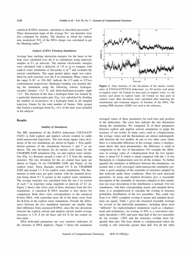
Stability of Simulations

The MD simulations of the B-DNA dodecamer CGCGAATT

CGCG in both explicit and implicit solvent resulted in stable

multi-nanosecond trajectories. The root mean square (rms) devi-

ations of the two simulations are shown in Figure 1. Post equili-

bration portions of the simulations between 1 and 7 ns are

shown. The rms deviations for all nucleic acid atoms for the

CHARMM ZAPI simulation (Fig. 1a) and explicit water simula-

tion (Fig. 1c) fluctuate around a value of 2 A from the starting

structure. The rms deviation for the six central base pairs are

shown in Figure 1b for CHARMM ZAPI and Figure 1d for

explicit water. These fluctuate around 0.9 A for CHARMM

ZAPI and around 1.3 A for explicit water simulations. The fluc-

tuations in both cases are quite similar, with the standard devia-

tion being about 0.1 A greater in the explicit water simulation.

The average structure was calculated from the last 5 ns section

of each 7 ns trajectory using snapshots at intervals of 0.1 ps.

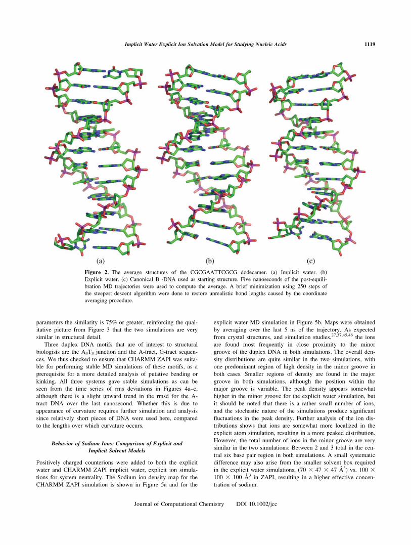
Figure 2 shows side views each of these structures from the two

simulations. A canonical B DNA structure is also shown for

comparison. Both show close correspondence to the canonical

B-form DNA, with somewhat more tilt of the bases away from

the B-form in the explicit water simulations. Overall, the differ-

ences between the two simulation structures are smaller than

their difference from canonical B-DNA, since the rms deviations

between the explicit solvent and implicit solvent model average

structures is 1.35 A for all bases and 0.8 A for the central six

base pairs.

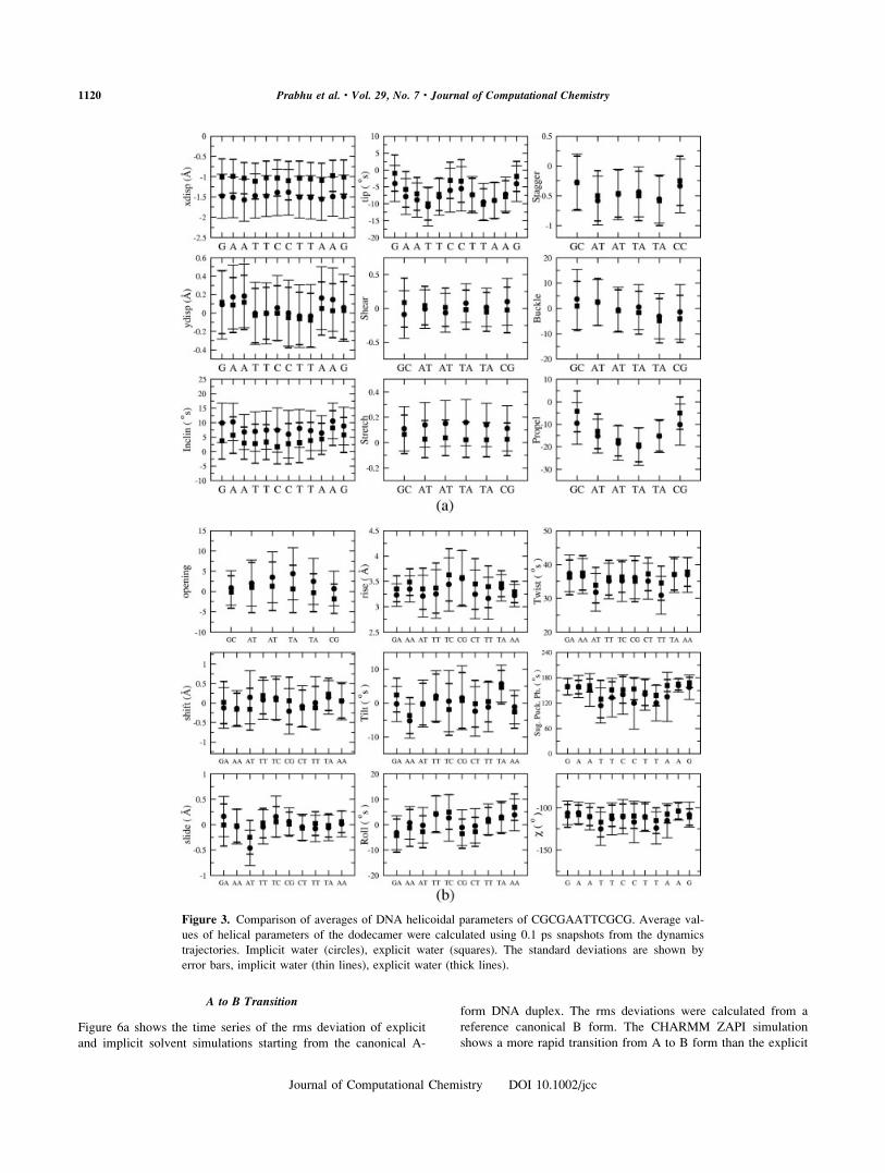
DNA helicoidal parameters are very sensitive indicators of

the structure of DNA duplexes. Figure 3 shows the simulation

averaged values of these parameters for each base pair position

in the dodecamer. The error bars indicate the rms fluctuation

during the simulations. We compared 24 of these parameters

between explicit and implicit solvent simulations to judge the

accuracy of our results. In many cases, such as y-displacement,

the average values and the fluctuations are almost indistinguish-

able between the two models. In one or two other cases where

there is a noticeable difference in the average values (x-displace-ment shows this most prominently), the difference is small in

comparison to the size of fluctuations. For example the differ-

ence in average value of x-displacement from the two simula-

tions is about 0.5 A which is small compared with the 1 A rms

fluctuation in x-displacement seen for all the residues. To further

quantify the similarity or difference between the simulations, we

assume that a well converged multi-nanosecond simulation pro-

vides a good sampling of the ensemble of structures adopted by

that molecule under those conditions. Then for each structural

parameter, its mean and standard deviation give a reasonable

description of the ensemble of structures adopted in that simula-

tion (an exact description if the distribution is normal). For two

simulations, with their corresponding means and standard devia-

tions, it is straightforward to calculate the overlap in structure

probability distributions of the two ensembles. This could vary

from 0 to 100% (complete overlap if means and standard devia-

tions are equal). Table 1 gives the structural ensemble overlaps

for several of the helicoidal parameters, including those most

‘‘different’’ for explicit/implicit simulations (such as x-displace-ment and inclination). An overlap of 50% is a convenient simi-

larity threshold (\50% and more than half of the two ensembles

do not overlap, [50% and the structures overlap more fre-

quently than not). The least similar is x-displacement where the

overlap is still somewhat greater than half. For all the other

Figure 1. Time histories of rms deviations of the atomic coordi-

nates of CGCGAATTCGCG dodecamer. (a) All nucleic acid atoms

in implicit water. (b) Central six base pairs in implicit water. (c) All

nucleic acid atoms in explicit water. (d) Central six base pairs in

explicit water. Rms deviations were calculated after removing the

translational and rotational degrees of freedom of the DNA. The

starting PDB structure (428D) was used as the reference.



parameters the similarity is 75% or greater, reinforcing the qual-

itative picture from Figure 3 that the two simulations are very

similar in structural detail.

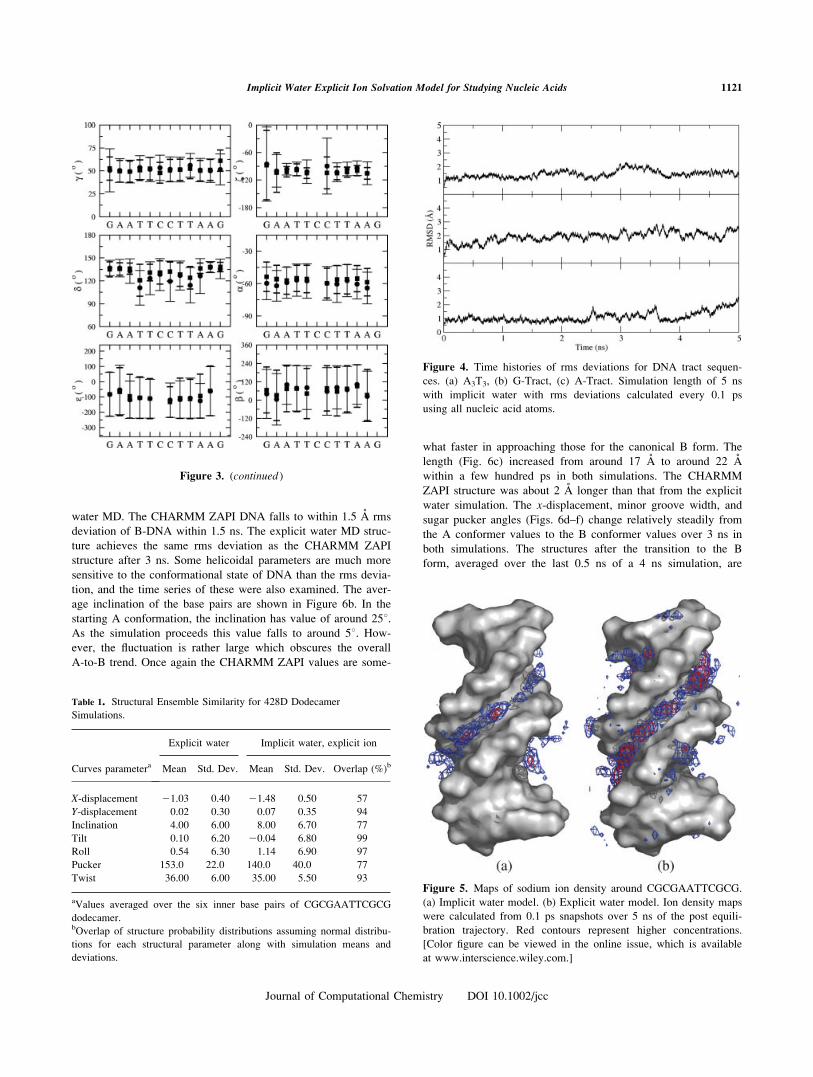
Three duplex DNA motifs that are of interest to structural

biologists are the A3T3 junction and the A-tract, G-tract sequen-

ces. We thus checked to ensure that CHARMM ZAPI was suita-

ble for performing stable MD simulations of these motifs, as a

prerequisite for a more detailed analysis of putative bending or

kinking. All three systems gave stable simulations as can be

seen from the time series of rms deviations in Figures 4a–c,

although there is a slight upward trend in the rmsd for the A-

tract DNA over the last nanosecond. Whether this is due to

appearance of curvature requires further simulation and analysis

since relatively short pieces of DNA were used here, compared

to the lengths over which curvature occurs.

Behavior of Sodium Ions: Comparison of Explicit and

Implicit Solvent Models

Positively charged counterions were added to both the explicit

water and CHARMM ZAPI implicit water, explicit ion simula-

tions for system neutrality. The Sodium ion density map for the

CHARMM ZAPI simulation is shown in Figure 5a and for the

explicit water MD simulation in Figure 5b. Maps were obtained

by averaging over the last 5 ns of the trajectory. As expected

from crystal structures, and simulation studies,27,37,45,46 the ions

are found most frequently in close proximity to the minor

groove of the duplex DNA in both simulations. The overall den-

sity distributions are quite similar in the two simulations, with

one predominant region of high density in the minor groove in

both cases. Smaller regions of density are found in the major

groove in both simulations, although the position within the

major groove is variable. The peak density appears somewhat

higher in the minor groove for the explicit water simulation, but

it should be noted that there is a rather small number of ions,

and the stochastic nature of the simulations produce significant

fluctuations in the peak density. Further analysis of the ion dis-

tributions shows that ions are somewhat more localized in the

explicit atom simulation, resulting in a more peaked distribution.

However, the total number of ions in the minor groove are very

similar in the two simulations: Between 2 and 3 total in the cen-

tral six base pair region in both simulations. A small systematic

difference may also arise from the smaller solvent box required

in the explicit water simulations, (70 3 47 3 47 A3) vs. 100 3100 3 100 A3 in ZAPI, resulting in a higher effective concen-

tration of sodium.

Figure 2. The average structures of the CGCGAATTCGCG dodecamer. (a) Implicit water. (b)

Explicit water. (c) Canonical B -DNA used as starting structure. Five nanoseconds of the post-equili-

bration MD trajectories were used to compute the average. A brief minimization using 250 steps of

the steepest descent algorithm were done to restore unrealistic bond lengths caused by the coordinate

averaging procedure.



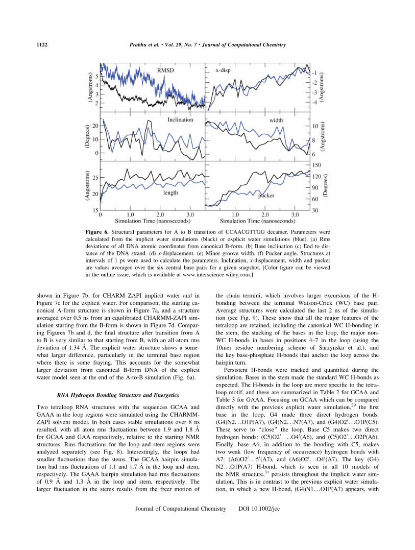
A to B Transition

Figure 6a shows the time series of the rms deviation of explicit

and implicit solvent simulations starting from the canonical A-

form DNA duplex. The rms deviations were calculated from a

reference canonical B form. The CHARMM ZAPI simulation

shows a more rapid transition from A to B form than the explicit

Figure 3. Comparison of averages of DNA helicoidal parameters of CGCGAATTCGCG. Average val-

ues of helical parameters of the dodecamer were calculated using 0.1 ps snapshots from the dynamics

trajectories. Implicit water (circles), explicit water (squares). The standard deviations are shown by

error bars, implicit water (thin lines), explicit water (thick lines).



water MD. The CHARMM ZAPI DNA falls to within 1.5 A rms

deviation of B-DNA within 1.5 ns. The explicit water MD struc-

ture achieves the same rms deviation as the CHARMM ZAPI

structure after 3 ns. Some helicoidal parameters are much more

sensitive to the conformational state of DNA than the rms devia-

tion, and the time series of these were also examined. The aver-

age inclination of the base pairs are shown in Figure 6b. In the

starting A conformation, the inclination has value of around 258.As the simulation proceeds this value falls to around 58. How-ever, the fluctuation is rather large which obscures the overall

A-to-B trend. Once again the CHARMM ZAPI values are some-

what faster in approaching those for the canonical B form. The

length (Fig. 6c) increased from around 17 A to around 22 A

within a few hundred ps in both simulations. The CHARMM

ZAPI structure was about 2 A longer than that from the explicit

water simulation. The x-displacement, minor groove width, and

sugar pucker angles (Figs. 6d–f) change relatively steadily from

the A conformer values to the B conformer values over 3 ns in

both simulations. The structures after the transition to the B

form, averaged over the last 0.5 ns of a 4 ns simulation, are

Figure 3. (continued )

Table 1. Structural Ensemble Similarity for 428D Dodecamer

Simulations.

Curves parametera

Explicit water Implicit water, explicit ion

Mean Std. Dev. Mean Std. Dev. Overlap (%)b

X-displacement 21.03 0.40 21.48 0.50 57

Y-displacement 0.02 0.30 0.07 0.35 94

Inclination 4.00 6.00 8.00 6.70 77

Tilt 0.10 6.20 20.04 6.80 99

Roll 0.54 6.30 1.14 6.90 97

Pucker 153.00 22.00 140.00 40.00 77

Twist 36.00 6.00 35.00 5.50 93

aValues averaged over the six inner base pairs of CGCGAATTCGCG

dodecamer.bOverlap of structure probability distributions assuming normal distribu-

tions for each structural parameter along with simulation means and

deviations.

Figure 4. Time histories of rms deviations for DNA tract sequen-

ces. (a) A3T3, (b) G-Tract, (c) A-Tract. Simulation length of 5 ns

with implicit water with rms deviations calculated every 0.1 ps

using all nucleic acid atoms.

Figure 5. Maps of sodium ion density around CGCGAATTCGCG.

(a) Implicit water model. (b) Explicit water model. Ion density maps

were calculated from 0.1 ps snapshots over 5 ns of the post equili-

bration trajectory. Red contours represent higher concentrations.

[Color figure can be viewed in the online issue, which is available

at www.interscience.wiley.com.]



shown in Figure 7b, for CHARM ZAPI implicit water and in

Figure 7c for the explicit water. For comparison, the starting ca-

nonical A-form structure is shown in Figure 7a, and a structure

averaged over 0.5 ns from an equilibrated CHARMM-ZAPI sim-

ulation starting from the B-form is shown in Figure 7d. Compar-

ing Figures 7b and d, the final structure after transition from A

to B is very similar to that starting from B, with an all-atom rms

deviation of 1.34 A. The explicit water structure shows a some-

what larger difference, particularly in the terminal base region

where there is some fraying. This accounts for the somewhat

larger deviation from canonical B-form DNA of the explicit

water model seen at the end of the A-to-B simulation (Fig. 6a).

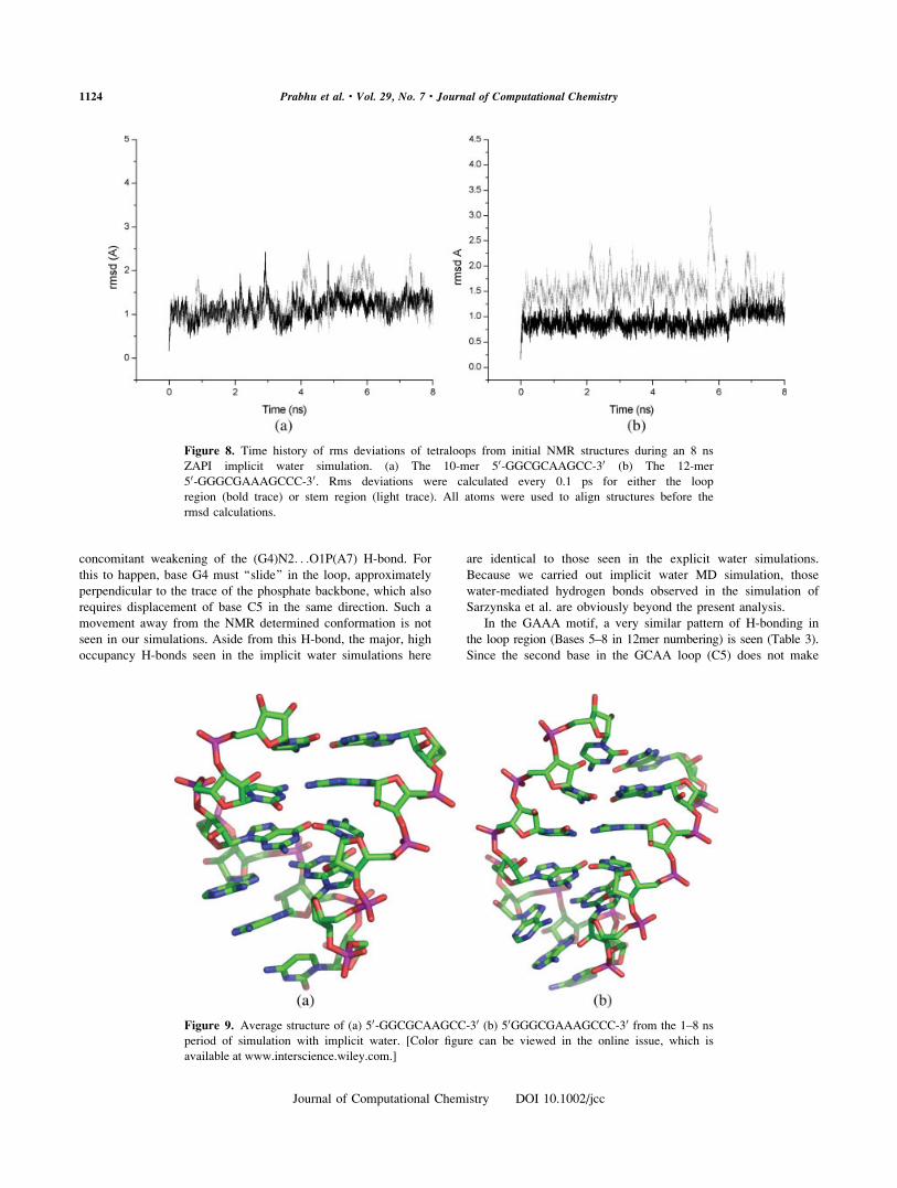
RNA Hydrogen Bonding Structure and Energetics

Two tetraloop RNA structures with the sequences GCAA and

GAAA in the loop regions were simulated using the CHARMM-

ZAPI solvent model. In both cases stable simulations over 8 ns

resulted, with all atom rms fluctuations between 1.9 and 1.8 A

for GCAA and GAA respectively, relative to the starting NMR

structures. Rms fluctuations for the loop and stem regions were

analyzed separately (see Fig. 8). Interestingly, the loops had

smaller fluctuations than the stems. The GCAA hairpin simula-

tion had rms fluctuations of 1.1 and 1.7 A in the loop and stem,

respectively. The GAAA hairpin simulation had rms fluctuations

of 0.9 A and 1.3 A in the loop and stem, respectively. The

larger fluctuation in the stems results from the freer motion of

the chain termini, which involves larger excursions of the H-

bonding between the terminal Watson-Crick (WC) base pair.

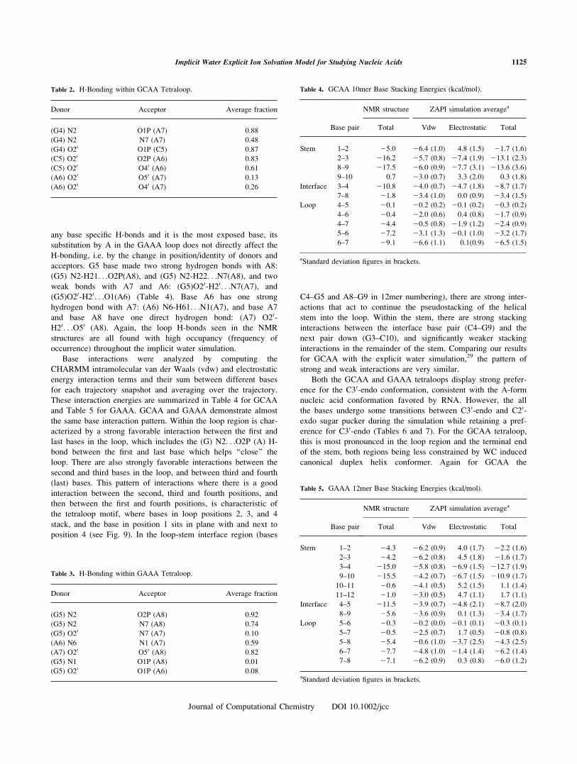
Average structures were calculated the last 2 ns of the simula-

tion (see Fig. 9). These show that all the major features of the

tetraloop are retained, including the canonical WC H-bonding in

the stem, the stacking of the bases in the loop, the major non-

WC H-bonds in bases in positions 4–7 in the loop (using the

10mer residue numbering scheme of Sarzynska et al.), and

the key base-phosphate H-bonds that anchor the loop across the

hairpin turn.

Persistent H-bonds were tracked and quantified during the

simulation. Bases in the stem made the standard WC H-bonds as

expected. The H-bonds in the loop are more specific to the tetra-

loop motif, and these are summarized in Table 2 for GCAA and

Table 3 for GAAA. Focusing on GCAA which can be compared

directly with the previous explicit water simulation,29 the first

base in the loop, G4 made three direct hydrogen bonds.

(G4)N2. . .O1P(A7), (G4)N2. . .N7(A7), and (G4)O20. . .O1P(C5).These serve to ‘‘close’’ the loop. Base C5 makes two direct

hydrogen bonds: (C5)O20 . . .O40(A6), and (C5)O20. . .O2P(A6).Finally, base A6, in addition to the bonding with C5, makes

two weak (low frequency of occurrence) hydrogen bonds with

A7: (A6)O20. . .50(A7), and (A6)O20. . .O40(A7). The key (G4)

N2. . .O1P(A7) H-bond, which is seen in all 10 models of

the NMR structure,31 persists throughout the implicit water sim-

ulation. This is in contrast to the previous explicit water simula-

tion, in which a new H-bond, (G4)N1. . .O1P(A7) appears, with

Figure 6. Structural parameters for A to B transition of CCAACGTTGG decamer. Parameters were

calculated from the implicit water simulations (black) or explicit water simulations (blue). (a) Rms

deviations of all DNA atomic coordinates from canonical B-form. (b) Base inclination (c) End to dis-

tance of the DNA strand. (d) x-displacement. (e) Minor groove width. (f) Pucker angle. Structures at

intervals of 1 ps were used to calculate the parameters. Inclination, x-displacement, width and pucker

are values averaged over the six central base pairs for a given snapshot. [Color figure can be viewed

in the online issue, which is available at www.interscience.wiley.com.]



Figure 7. A to B transition of CCAACGTTGG decamer. (a) A-form conformation used to initialize

the simulations. (b) Average structure over the 3.5–4 ns period of the simulation using implicit water.

(c) Average structure over the 3.5–4 ns period of simulation with explicit water. (d) Average structure

over 1 ns starting from the B-form, using implicit water. [Color figure can be viewed in the online

issue, which is available at www.interscience.wiley.com.]



concomitant weakening of the (G4)N2. . .O1P(A7) H-bond. For

this to happen, base G4 must ‘‘slide’’ in the loop, approximately

perpendicular to the trace of the phosphate backbone, which also

requires displacement of base C5 in the same direction. Such a

movement away from the NMR determined conformation is not

seen in our simulations. Aside from this H-bond, the major, high

occupancy H-bonds seen in the implicit water simulations here

are identical to those seen in the explicit water simulations.

Because we carried out implicit water MD simulation, those

water-mediated hydrogen bonds observed in the simulation of

Sarzynska et al. are obviously beyond the present analysis.

In the GAAA motif, a very similar pattern of H-bonding in

the loop region (Bases 5–8 in 12mer numbering) is seen (Table 3).

Since the second base in the GCAA loop (C5) does not make

Figure 8. Time history of rms deviations of tetraloops from initial NMR structures during an 8 ns

ZAPI implicit water simulation. (a) The 10-mer 50-GGCGCAAGCC-30 (b) The 12-mer

50-GGGCGAAAGCCC-30. Rms deviations were calculated every 0.1 ps for either the loop

region (bold trace) or stem region (light trace). All atoms were used to align structures before the

rmsd calculations.

Figure 9. Average structure of (a) 50-GGCGCAAGCC-30 (b) 50GGGCGAAAGCCC-30 from the 1–8 ns

period of simulation with implicit water. [Color figure can be viewed in the online issue, which is

available at www.interscience.wiley.com.]



any base specific H-bonds and it is the most exposed base, its

substitution by A in the GAAA loop does not directly affect the

H-bonding, i.e. by the change in position/identity of donors and

acceptors. G5 base made two strong hydrogen bonds with A8:

(G5) N2-H21. . .O2P(A8), and (G5) N2-H22. . .N7(A8), and two

weak bonds with A7 and A6: (G5)O20-H20. . .N7(A7), and

(G5)O20-H20. . .O1(A6) (Table 4). Base A6 has one strong

hydrogen bond with A7: (A6) N6-H61. . .N1(A7), and base A7

and base A8 have one direct hydrogen bond: (A7) O20-H20. . .O50 (A8). Again, the loop H-bonds seen in the NMR

structures are all found with high occupancy (frequency of

occurrence) throughout the implicit water simulation.

Base interactions were analyzed by computing the

CHARMM intramolecular van der Waals (vdw) and electrostatic

energy interaction terms and their sum between different bases

for each trajectory snapshot and averaging over the trajectory.

These interaction energies are summarized in Table 4 for GCAA

and Table 5 for GAAA. GCAA and GAAA demonstrate almost

the same base interaction pattern. Within the loop region is char-

acterized by a strong favorable interaction between the first and

last bases in the loop, which includes the (G) N2. . .O2P (A) H-

bond between the first and last base which helps ‘‘close’’ the

loop. There are also strongly favorable interactions between the

second and third bases in the loop, and between third and fourth

(last) bases. This pattern of interactions where there is a good

interaction between the second, third and fourth positions, and

then between the first and fourth positions, is characteristic of

the tetraloop motif, where bases in loop positions 2, 3, and 4

stack, and the base in position 1 sits in plane with and next to

position 4 (see Fig. 9). In the loop-stem interface region (bases

C4–G5 and A8–G9 in 12mer numbering), there are strong inter-

actions that act to continue the pseudostacking of the helical

stem into the loop. Within the stem, there are strong stacking

interactions between the interface base pair (C4–G9) and the

next pair down (G3–C10), and significantly weaker stacking

interactions in the remainder of the stem. Comparing our results

for GCAA with the explicit water simulation,29 the pattern of

strong and weak interactions are very similar.

Both the GCAA and GAAA tetraloops display strong prefer-

ence for the C30-endo conformation, consistent with the A-form

nucleic acid conformation favored by RNA. However, the all

the bases undergo some transitions between C30-endo and C20-exdo sugar pucker during the simulation while retaining a pref-

erence for C30-endo (Tables 6 and 7). For the GCAA tetraloop,

this is most pronounced in the loop region and the terminal end

of the stem, both regions being less constrained by WC induced

canonical duplex helix conformer. Again for GCAA the

Table 2. H-Bonding within GCAA Tetraloop.

Donor Acceptor Average fraction

(G4) N2 O1P (A7) 0.88

(G4) N2 N7 (A7) 0.48

(G4) O20 O1P (C5) 0.87

(C5) O20 O2P (A6) 0.83

(C5) O20 O40 (A6) 0.61

(A6) O20 O50 (A7) 0.13

(A6) O20 O40 (A7) 0.26

Table 3. H-Bonding within GAAA Tetraloop.

Donor Acceptor Average fraction

(G5) N2 O2P (A8) 0.92

(G5) N2 N7 (A8) 0.74

(G5) O20 N7 (A7) 0.10

(A6) N6 N1 (A7) 0.59

(A7) O20 O50 (A8) 0.82

(G5) N1 O1P (A8) 0.01

(G5) O20 O1P (A6) 0.08

Table 4. GCAA 10mer Base Stacking Energies (kcal/mol).

Base pair

NMR structure ZAPI simulation averagea

Total Vdw Electrostatic Total

Stem 1–2 25.0 26.4 (1.0) 4.8 (1.5) 21.7 (1.6)

2–3 216.2 25.7 (0.8) 27.4 (1.9) 213.1 (2.3)

8–9 217.5 26.0 (0.9) 27.7 (3.1) 213.6 (3.6)

9–10 0.7 23.0 (0.7) 3.3 (2.0) 0.3 (1.8)

Interface 3–4 210.8 24.0 (0.7) 24.7 (1.8) 28.7 (1.7)

7–8 21.8 23.4 (1.0) 0.0 (0.9) 23.4 (1.5)

Loop 4–5 20.1 20.2 (0.2) 20.1 (0.2) 20.3 (0.2)

4–6 20.4 22.0 (0.6) 0.4 (0.8) 21.7 (0.9)

4–7 24.4 20.5 (0.8) 21.9 (1.2) 22.4 (0.9)

5–6 27.2 23.1 (1.3) 20.1 (1.0) 23.2 (1.7)

6–7 29.1 26.6 (1.1) 0.1(0.9) 26.5 (1.5)

aStandard deviation figures in brackets.

Table 5. GAAA 12mer Base Stacking Energies (kcal/mol).

Base pair

NMR structure ZAPI simulation averagea

Total Vdw Electrostatic Total

Stem 1–2 24.3 26.2 (0.9) 4.0 (1.7) 22.2 (1.6)

2–3 24.2 26.2 (0.8) 4.5 (1.8) 21.6 (1.7)

3–4 215.0 25.8 (0.8) 26.9 (1.5) 212.7 (1.9)

9–10 215.5 24.2 (0.7) 26.7 (1.5) 210.9 (1.7)

10–11 20.6 24.1 (0.5) 5.2 (1.5) 1.1 (1.4)

11–12 21.0 23.0 (0.5) 4.7 (1.1) 1.7 (1.1)

Interface 4–5 211.5 23.9 (0.7) 24.8 (2.1) 28.7 (2.0)

8–9 25.6 23.6 (0.9) 0.1 (1.3) 23.4 (1.7)

Loop 5–6 20.3 20.2 (0.0) 20.1 (0.1) 20.3 (0.1)

5–7 20.5 22.5 (0.7) 1.7 (0.5) 20.8 (0.8)

5–8 25.4 20.6 (1.0) 23.7 (2.5) 24.3 (2.5)

6–7 27.7 24.8 (1.0) 21.4 (1.4) 26.2 (1.4)

7–8 27.1 26.2 (0.9) 0.3 (0.8) 26.0 (1.2)

aStandard deviation figures in brackets.



observed results are consistent with the explicit water simula-

tions.29

Salt Solutions

Simulations at all NaCl concentrations from 10 to 500 mM gave

stable simulations, as judged by the rmsd which, although it

fluctuated from about 1.5 to 3.5 A over the last 3 ns of the sim-

ulation (Table 8), showed no long term upward trend. Basic pa-

rameters for the ion concentration profiles are given in Table 8.

One measure of the width of the ion atmosphere around DNA is

the radius rm within which the Manning fraction of the net DNA

charge is neutralized. For B-DNA this fraction is 76%.44 As the

ionic strength is increased from 10 to 500 mM rm decreases

from [30 to 19 A, similar to that obtained in previous studies

of B-DNA, and to that obtained from the mean field NLPB

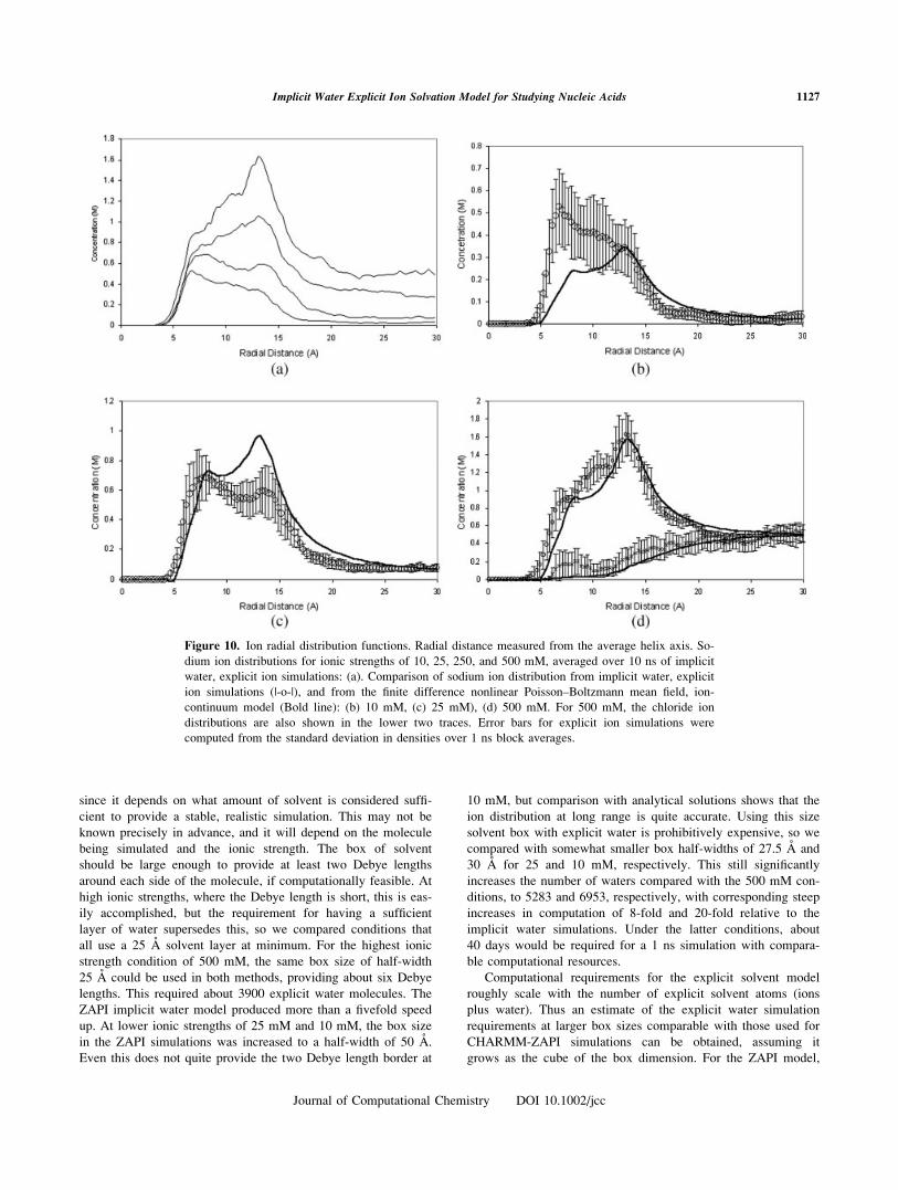
model. A more detailed structural picture of the ion atmosphere

is provided by the sodium ion radial distribution function. Fig-

ure 10a shows the distribution of ions as function of distance

from the DNA helical axis for salt concentrations of 10, 25,

250, and 500 mM. The sodium ions in all cases have a high

density in the region 7–15 A from the helix axis and approach

the bulk value by a radius of 20–30 A, except for the 10 mM

case. Here and the ion concentrations are still 2–3 fold higher

than bulk at ZAP box cut off of 30 A as expected since the

Debye length is 30 A. Interestingly, the position of the maximum in

sodium ion density changes as the ionic strength is lowered. At

high ionic strength ([250 m) it occurs at 13 A (Table 8), corre-

sponding to a position midway between the phosphates in the minor

groove (Fig. 11b). As the ionic strength is lowered, a peak of den-

sity builds up at 7–8 A, corresponding to accumulation of ions at

the base of the major groove (Fig. 11a) producing a bimodal distri-

bution at intermediate to low salt concentrations. The chloride ion

profile is low near DNA and monotonically approaches the bulk

value at larger radii. Virtually identical profiles for chloride are

seen for all salt concentrations, and are only shown for 500 mM in

Figure 10d. The sodium ion distributions at 10, 25, and 500 mM

for explicit ion CHARMM-ZAPI and mean field continuum ion

atmosphere NLPB models are compared in Figures 10b–d. At

high salt the ion distributions are virtually identical in the two

models, within experimental uncertainty. This implies that any ion

discreteness and ion correlation effects are small at the higher con-

centrations: In effect they are averaged out because of the high

density of ions everywhere, so that the distribution looks like that

of the continuum model. At lower salt concentrations, however,

the explicit ion model shows increasing accumulation of sodium

ions in the major groove, unlike the ion continuum model which

has essentially the same shape profile at all concentrations. This

indicates that discrete ion effects become significant at lower ion

concentrations. This is expected on physical grounds, when ion

separations frequently exceed the bjerrum length (7 A at 298 K

and a water dielectric of 80).

Computational Requirements

Table 9 presents relative timings for the CHARMM-ZAPI

implementation of the implicit water model versus the standard

CHARMM-TIP3P explicit water treatment. Both models treat

ions explicitly. Making timing comparisons is somewhat inexact

Table 6. GCAA 10mer Sugar Conformations.

Base

NMR structure Simulation average (%)

Phase angle (8) Sugar pucker C3 endo C2 exo

G1 2 C30-endo 80 19

G2 9 C30-endo 90 10

C3 2 C30-endo 93 5

G4 357 C20-exo 80 20

C5 358 C20-exo 64 36

A6 6 C30-endo 75 25

A7 359 C20-exo 87 10

G8 7 C30-endo 78 22

C9 2 C30-endo 85 15

C10 7 C30-endo 67 20

Table 7. GAAA 12mer Sugar Conformations.

Base

NMR structure Simulation average (%)

Phase angle (8) Sugar pucker C3 endo C2 exo

G1 23 C30-endo 80 20

G2 13 C30-endo 96 4

G3 7 C30-endo 78 22

C4 348 C20-exo 88 12

G5 9 C30-endo 92 7

A6 13 C30-endo 93 7

A7 28 C30-endo 80 20

A8 349 C20-exo 81 19

G9 360 C20-exo 85 15

C10 351 C20-exo 90 10

C11 354 C20-exo 43 57

C12 4 C30-endo 59 41

Table 8. Comparison of Ion Distributions.

[NaCl]

(mM)

rmsd

(A)a

Cmax mM

(at radius, A)b r0.76 (A)c

Charmm-

ZAPId NLPB

Charmm-

ZAPI NLPB

10 1.1–3.6 0.5 (7) 0.35 (13) [30 29

25 1.3–3.3 0.7 (8) 0.97 (13) [30 27

250 1.6–3.7 1.0 (13) 1.3 (13) 18 17

500 1.1–3.8 1.6 (13) 1.56 (13) 19 15

aRange of all atom root mean square deviations from canonical B-DNA

structure over last 3 ns of Charmm-ZAPI simulation.bMaximum in radially averaged Na1 concentration and distance from

helical axis at which it occurs.cDistance at which Manning fraction of 76% of phosphate charged is

neutralized by Na1.dCharmm-ZAPI: average values from 10 ns of simulation. NLPB: finite

difference solutions to nonlinear Poisson-Boltzmann equation.



since it depends on what amount of solvent is considered suffi-

cient to provide a stable, realistic simulation. This may not be

known precisely in advance, and it will depend on the molecule

being simulated and the ionic strength. The box of solvent

should be large enough to provide at least two Debye lengths

around each side of the molecule, if computationally feasible. At

high ionic strengths, where the Debye length is short, this is eas-

ily accomplished, but the requirement for having a sufficient

layer of water supersedes this, so we compared conditions that

all use a 25 A solvent layer at minimum. For the highest ionic

strength condition of 500 mM, the same box size of half-width

25 A could be used in both methods, providing about six Debye

lengths. This required about 3900 explicit water molecules. The

ZAPI implicit water model produced more than a fivefold speed

up. At lower ionic strengths of 25 mM and 10 mM, the box size

in the ZAPI simulations was increased to a half-width of 50 A.

Even this does not quite provide the two Debye length border at

10 mM, but comparison with analytical solutions shows that the

ion distribution at long range is quite accurate. Using this size

solvent box with explicit water is prohibitively expensive, so we

compared with somewhat smaller box half-widths of 27.5 A and

30 A for 25 and 10 mM, respectively. This still significantly

increases the number of waters compared with the 500 mM con-

ditions, to 5283 and 6953, respectively, with corresponding steep

increases in computation of 8-fold and 20-fold relative to the

implicit water simulations. Under the latter conditions, about

40 days would be required for a 1 ns simulation with compara-

ble computational resources.

Computational requirements for the explicit solvent model

roughly scale with the number of explicit solvent atoms (ions

plus water). Thus an estimate of the explicit water simulation

requirements at larger box sizes comparable with those used for

CHARMM-ZAPI simulations can be obtained, assuming it

grows as the cube of the box dimension. For the ZAPI model,

Figure 10. Ion radial distribution functions. Radial distance measured from the average helix axis. So-

dium ion distributions for ionic strengths of 10, 25, 250, and 500 mM, averaged over 10 ns of implicit

water, explicit ion simulations: (a). Comparison of sodium ion distribution from implicit water, explicit

ion simulations (|-o-|), and from the finite difference nonlinear Poisson–Boltzmann mean field, ion-

continuum model (Bold line): (b) 10 mM, (c) 25 mM), (d) 500 mM. For 500 mM, the chloride ion

distributions are also shown in the lower two traces. Error bars for explicit ion simulations were

computed from the standard deviation in densities over 1 ns block averages.



requirements depend on both the number of explicit ions and the

box size. However, for low ionic strengths, the FDP treatment is

applied only to an inner region of the box, no larger than a half-

width of 30 A. Ions in the rest of the box are treated by the

inexpensive Coulombic model, so beyond a half-width of 30 A

the computational requirements depend principally on the num-

ber of ions. Thus computation times at both low ionic strength

(large box, but few ions, most treated Coulombically) and at

high ionic strength (somewhat more ions, but limited by the

smaller box) are similar and relatively modest. Overall, the

results show the implicit water model would provide significant,

many-fold speedups compared with the explicit water treatment

over a range of ionic strengths.

Discussion

In this work, we have extended our previous finite difference

Poisson–Boltzmann implicit water solvent model to the MD sim-

ulation of highly charged nucleic acids. The model gives stable

simulations for a variety of nucleic acids molecules, including

canonical B-DNA dodecamers and decamers, and tetraloop

RNA. Detailed comparison with explicit water simulations of B-

DNA shows very similar results: Analysis using the CURVES

DNA structural analysis program shows that all 24 helicoidal

and base parameters show either no statistically significant dif-

ference or, for two parameters, differences that lie well within

the normal fluctuations of the simulation. The distribution of

neutralizing sodium ions is also very similar for explicit water

and implicit water simulations. Stable simulations are also

obtained for a variety of different base sequences. The implicit

water model simulates the A to B transition accurately. Compar-

ison of the A to B transition between explicit and implicit water

simulations shows very similar structural changes and similar

final stable B-DNA structures, although the transition happens

about 2–3 times faster with implicit water. This result is compa-

rable with a previous GB implicit solvent model study of the A

to B transition, which also found faster transition with implicit

water. Comparison of our implicit water simulations of tetraloop

RNA with NMR structures and previous explicit water simula-

tions shows good correspondence of general structural features,

as well as detailed structural features like individual H-bonds,

and energetic terms. For one particular important H-bond, our

implicit water model actually stays closer to the experimental

NMR structure than the explicit solvent model, although not too

much significance should be attached to the more accurate mod-

eling of a single H-bond among many.

A significant extension of our implicit solvent model is the

explicit treatment of ions. In contrast to other previous implicit

water models, including the Deby–Huckel modified GB model,19

here only the water molecules, not the ions, are treated implic-

itly. This allows us to incorporate the nonlinear ion atmosphere

response, discrete finite size ion effects, and the resulting corre-

lations between ion positions. This is achieved with only a mod-

est increase in the number of explicit atoms represented in the

simulations. This allows us for the first time to perform system-

atic studies of the MD of DNA and RNA with a wide range of

well defined ionic strengths, good convergence of ion atmos-

phere structure, and tractable computation times. The results

Table 9. Relative Timings.

Ionic strength

(mM)

Debye

length (A)

Water

model

Number of ions

No. of

TIP3P waters

1/2 Box

width rb (A)

Cpu

timea (s)

Relative

speedbNa1 Cl2

10 30 ZAPI 12 2 nac 50 172 1

25 20 ZAPI 44 27 na 50 310 1

500 4 ZAPI 48 30 na 25 170 1

10 30 Explicit 8 0 6953 30 3456 20

25 20 Explicit 20 6 5283 27.5 2448 8

500 4 Explicit 48 30 3898 25 933 5.5

aCPU time for 1ps of simulation on a 2.8 GHz Xeon processor, with 1 Gb RAM, running under Linux 9.1.bCPU time required relative to implicit solvent simulation at corresponding ionic strength.cna: not applicable.

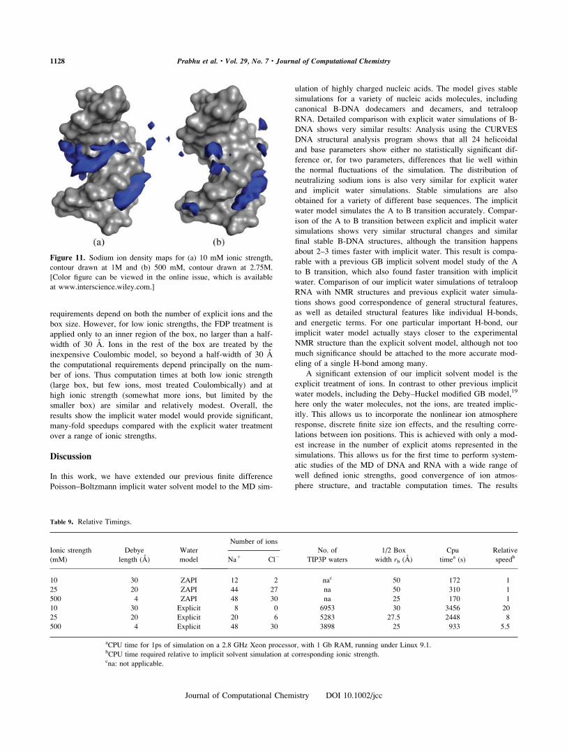
Figure 11. Sodium ion density maps for (a) 10 mM ionic strength,

contour drawn at 1M and (b) 500 mM, contour drawn at 2.75M.

[Color figure can be viewed in the online issue, which is available

at www.interscience.wiley.com.]



demonstrate that at high ionic strength (500 mM), the sodium ion

distributions are strikingly very similar for explicit ion and

implicit ion mean field models. For the neutralizing sodium, no

added salt case, very similar ion distributions are obtained for

explicit water and implicit water models. Both results provide a

check on the correctness of the CHARMM-ZAPI implementation

of the explicit ion model. Moreover, the close correspondence of

sodium ion distributions in the CHARMM-ZAPI and NLPB mod-

els for I 5 250–500 mM shows that the mean field continuum

ion atmosphere NLPB model may be used with some confidence

to model ion atmospheres in this salt range, at least for 1-1 salts.

At lower salt concentrations, however, it appears that discrete ion

effects produce quite different distributions of sodium ions, with

significant ions accumulating in the major groove.

Exact comparison with other studies of ionic strength de-

pendence of the ion atmosphere around DNA is difficult. The

majority of previous studies have used mean field models like

the NLPB or counter-ion condensation models. A systematic ex-

amination of range of ionic strength is easily performed with

these models. Indeed this class of model is what we have com-

pared to here in Figure 10. However, these models do not ex-

plicitly include the effects of DNA structural fluctuations, nor

discrete ion effects. Notably, one study of this type has incorpo-

rated ion-correlation effects around a fixed all atom model of

DNA at two concentrations, 0.1M and 5M.47 At the lower con-

centration there is a bimodal distribution of sodium ions with

peaks at 8 and 14 A, very similar to that seen here. There is

more separation of peaks in the study of Klement et al., prob-

ably a consequence of using fixed DNA. DNA fluctuations

included here have effect of broadening the distributions, and

making the separation between the peaks less distinct. The other

major method used to study DNA is with all atom DNA, explicit

ion, explicit water models, using MD simulations. The majority

of these have been done with just neutralizing counterions (usu-

ally sodium), which loosely corresponds to low ionic strength

conditions, but with rather small solvent boxes. The major rea-

son is technical difficulties: To simulate, for example, an ionic

strength of 10 mM with a Debye length of 30 A, one needs at

least two Debye lengths of solvent around each side of DNA,

requiring a box of dimension 120 A and about 57,000 explicit

waters. Given typical ion diffusion constants of 100–200 A2/ns

the characteristic relaxation time of this ion atmosphere would

be about 5 ns. Thus one requires very large, long simulations.

Ponomarev et al.48 presented benchmark simulations in this

regard, using a DNA decamer with 3949 waters and 22 neutral-

izing sodium ions. They did 60 ns of simulations, requiring

6 months, to ensure convergence in ion atmosphere features.

Although their analysis indicated that ion radial distributions

may converge in about 5 ns, and ion occupancies may converge

in about 14 ns, it is clearly still computationally challenging to

do systematic ionic strength simulations with explicit water. The

results of Ponomarev et al.48 also show a bimodal distribution of

sodium ions, with accumlation in the base of the major groove

in addition to the well documented spine of ions positions

between phosphates in the minor groove. A review of other such

MD simulations by Lyubartsov37 also documents bimodal ion

distributions at 8 and 12 A, in agreement with the implicit

water, explicit ion model here. In explicit water simulations at

higher ionic strengths of about 0.2M by Bonvin49 there is lesser,

and discontinuous sodium ion accumulation in the major groove,

most being in the minor groove. Taking these results together

with ours, a consistent picture emerges. Cations accumulate pref-

erentially in both grooves at low ionic strengths, with a prefer-

ence for positioning deeper into the major groove, while at

higher ionic strength cations accumulate preferentially in the

minor groove, positioned midway between the phosphate groups

of opposite strands. It should be stressed though, that these state-

ments about distributions reflect preferences between major or

minor grooves at a given ionic strength. At high ionic strengths

the net concentration of ions in the major groove, although less

than that in the minor groove, is still greater that that in the

major groove at lower ionic strength (e.g., see Fig. 10a).

It is clear from comparison of the NLPB implicit ion model

and the CHARMM-ZAPI explicit ion model that the greater

accumulation of cations in the major groove results from dis-

crete ion effects, but it is not clear why. Representation of

explicit ions introduces three physical factors not present in

mean field continuum ion models. (1) Positional correlation

effects. The probability of finding one ion near another is lower

(for same charge ions) or higher (for opposite charge ions) in a

discrete ion model than in a mean field model (2) Finite size

effects. This penalizes close ion-to-ion distances. (3) Born-like

desolvation effects. As an ion approaches the low dielectric

DNA it experiences a desolvation penalty inversely proportional

to its radius. Which of these factors is responsible is not clear at

this point. However, this is a logical direction for future study

which is now made feasible by the CHARMM-ZAPI model.

Simulations were performed here using fixed ion concentra-

tions set to reproduce specified ionic strengths. However, the

explicit ion-implicit water model also holds out the promise of

doing efficient semi-grand canonical simulations at constant ion

activity, simultaneously with an all atom dynamic model of

DNA, and realistic solvent dielectric effects. Such semi-grand

simulations involve sampling moves that insert or remove ions

at a given ion activity, as has been done using the primitive ion-

electrostatic model for fixed DNA.50 This would be difficult

with explicit water simulations as insertion moves involve dis-

placing water molecules. Generating an ion-cavity water config-

uration of acceptable low energy for insertion is improbable.

This leads to very inefficient sampling and poor convergence. In

contrast, ion insertion would be much easier with the implicit

water, explicit ion model developed here, since a fixed Born self

energy/ion activity term is simply added to the CHARRM force-

field energy change upon insertion.

In summary, we have developed, tested, and made prelimi-

nary application of an implicit water explicit ion solvation

model for studying nucleic acids. We have shown that the model

yields long stable simulations on a variety of nucleic acid mole-

cules, and it provides very similar results to explicit water simu-

lations with a fraction of the computational expense. The model

treats ions explicitly, avoiding the approximations made in mean

field ion-continuum electrostatic models. The method makes MD

simulations at a range of well-defined ionic strengths computa-

tionally feasible. This now permits the systematic study of ionic

strength on nucleic acid structure in MD simulations. The first

applications already clearly show where mean field ion and



explicit ion effects differ, and demonstrate how the ion atmos-

phere structure around B-DNA changes with salt concentration.

Acknowledgments

We thank Miler Lee for writing a high throughput front end to

the CURVES program.

References

1. Bashford, D.; Case, D. Ann Rev Phys Chem 2000, 51, 129.

2. Simonson, T. Curr Opin Struct Biol 2001, 11, 243.

3. Davis, M. E.; McCammon, J. A. J Comput Chem 1990, 11, 401.

4. Sharp, K. A. J Comput Chem 1991, 12, 454.

5. Zauhar, R. J Comput Chem 1991, 12, 575.

6. Niedermeier, C.; Schulten, K. Mol Simul 1992, 8, 361.

7. Gilson, M.; Davis, M.; Luty, B.; McCammon, J. J Phys Chem 1993,

97, 3591.

8. Gilson, M.; Davis, M.; Luty, B.; Madura, J.; McCammon, J. Biophys

J 1993, 64, A 354.

9. Madura, J.; Gilson, M. Biophys J 1993, 64, A 220.

10. Lu, Q.; Luo, R. J Chem Phys 2003, 119, 11035.

11. Prabhu, N. V.; Zhu, P.-J.; Sharp, K. A. J Comput Chem 2004, 25,

2049.

12. Still, C.; Tempczyk, A.; Hawley, R.; Hendrickson, T. J Am Chem

Soc 1990, 112, 6127.

13. Calimet, N.; Schaeffer, M.; Simonson, T. Proteins 2001, 45, 144.

14. Dominy, B.; Brooks, C. J Phys Chem B 1999, 103, 3765.

15. Jayaram, B.; Sprous, D.; Beveridge, D. L. J Phys Chem B 1998,

102, 9571.

16. Lee, M. S.; Salsbury, F. R., Jr.; Brooks, C. L., III. J Chem Phys

2002, 116, 10606.

17. Onufriev, A.; Bashford, D.; Case, D. A. J Phys Chem B 2000, 104,

3712.

18. Qui, D.; Shenkin, P.; Hollinger, F.; Still, W. J Phys Chem 1997,

101, 3005–3014.

19. Tsui, V.; Case, D. JACS 2000, 122, 2489.

20. Gallicchio, E.; Levy, R. M. J Comput Chem 2004, 25, 479.

21. Feig, M.; Im, W.; Brooks, C. L. J Chem Phys 2004, 120, 903.

22. Sharp, K.; Honig, B. J Phys Chem 1990, 94, 7684.

23. Srinivasan, J.; Trevathan, M. W.; Beroza, P.; Case, D. A. Theor

Chem Acc 1999, 101, 426.

24. Tsui, V.; Case, D. A. J Phys Chem B 2001, 105, 11314.

25. Wojciechowski, M.; Lesyng, B. J Phys Chem B 2004, 108, 18368.

26. Edwards, K. J.; Brown, D. G.; Spink, N.; Skelly, J. V.; Neidle, S. J

Mol Biol 1992, 226, 1161.

27. Shui, X.; Sines, C. C.; McFail-Isom, L.; VanDerveer, D.; Williams,

L. D. Biochemistry 1998, 37, 16877.

28. Case, D.; Pearlman, D.; Caldwell, J. W.; Cheatham, T.; Wang, J.;

Ross, C.; Simmerling, T.; Darden, T.; Merz, K.; Stanton, A.; Chenn,

J.; Vincent, M.; Crowley, V.; Crowley, V.; Tsui, V.; Gohlke, H.;

Radmer, R.; Duan, Y.; Pitera, J.; Massova, I.; Seibel, G.; Singh, U.;

Weiner, P.; Kollman, P. A.; AMBER 7, UCSF, 2002.

29. Sarzynska, J.; Nilsson, L.; Kulinski, T. Biophys J 2003, 85, 3445.

30. Eric, J. S.; Engelhardt M. A.; Herschlag D.; Pande V. S. J Mol Biol

2002, 317, 493.

31. Jucker, F. M.; Heus H. A.; Yip P. F.; Moors E. H. M.; Pardi A. J

Mol Biol 1996, 264, 968.

32. Ryckaert, J. P.; Ciccotti, G.; Berendsen, H. J. C. Numer J Comp

Chem 1977, 23, 327.

33. Konerding, D. E.; Cheatham, T. E.; Kollman, P. A.; James, T. L. J

Biomol NMR 1999, 13, 119.

34. MacKerell, A. D.; Brooks, B.; Brooks, C. L.; Nilsson, L.; Roux, B.;

Won, Y.; Karplus, M. In The Encyclopedia of Computational Chem-

istry; Schleyer, P. V. R., Ed.; John Wiley & Sons: Chichester, 1998,

pp 271–277.

35. Brooks, B. R.; Bruccoleri, R. E.; Olafson, B. D.; States, D. J.; Swa-

minathan, S.; Karplus, M. J Comput Chem 1983, 4, 187.

36. Sharp, K. A. Biopolymers 1995, 36, 227.

37. Lyubartsov, A. In Dekker Encyclopedia of Nanoscience and Nano-

technology; New York: Marcel Dekker, 2004.

38. Jayaram, B.; Swaminathan, S.; Beveridge, D. L.; Sharp, K.; Honig,

B. Macromolecules 1990, 23, 3156.

39. Aqvist, J. J Phys Chem 1990, 94, 8021.

40. Sridharan, S.; Nicholls, A.; Sharp, K. A. J Comput Chem 1995, 16,

1038.

41. Lavery, R.; Sklenar, H. J Biomol Struct Dyn 1988, 6, 63.

42. Lavery, R.; Sklenar, H. J Biomol Struct Dyn 1989, 6, 655.

43. Jayaram, B.; Sharp, K. A.; Honig, B. Biopolymers 1989, 28, 975.

44. Manning, G. J Phys Chem 1969, 51, 924.

45. Young, M. A.; Jayaram, B.; Beveridge, D. L. J Am Chem Soc 1997,

119, 59.

46. Hamelberg, D.; McFail-Isom, L.; Williams, L. D.; Wilson, W. D.

JACS 2000, 122, 10513.

47. Klement, R.; Soumpasis, D.; Jovin, T. Proc Natl Acad Sci USA

1991, 88, 4631.

48. Ponomarev, S.; Thayer, K.; Beveridge, D. L. Proc Natl Acad Sci

USA 2004, 101, 14771.

49. Bonvin, A. Eur Biophys J 2000, 29, 57.

50. Olmsted, M. C.; Anderson, C. F.; Record, M. T. Proc Natl Acad Sci

USA 1989, 86, 7766.



Documents

Explicit Ion, Implicit Water Solvation for Molecular ...crystal.med.upenn.edu/sharp-lab-pdfs/prabhu_zapdna_Jcompchem_2… · Explicit Ion, Implicit Water Solvation for Molecular Dynamics