Embed Size (px)
Citation preview
Noname manuscript No.(will be inserted by the editor)
Explanation-Based Large Neighborhood Search
Charles Prud’homme · Xavier Lorca ·Narendra Jussien
Received: date / Accepted: date
Abstract One of the most well-known and widely used local search techniquesfor solving optimization problems in Constraint Programming is the Large Neigh-borhood Search (LNS) algorithm. Such a technique is, by nature, very flexibleand can be easily integrated within standard backtracking procedures. One of itsdrawbacks is that the relaxation process is quite often problem dependent. Severalworks have been dedicated to overcome this issue through problem independentparameters. Nevertheless, such generic approaches need to be carefully parameter-ized at the instance level. In this paper, we demonstrate that the issue of finding aproblem independent neighborhood generation technique for LNS can be addressedusing explanation-based neighborhoods. An explanation is a subset of constraintsand decisions which justifies a solver event such as a domain modification or aconflict. We evaluate our proposal for a set of optimization problems. We showthat our approach is at least competitive with or even better than state-of-the-artalgorithms and can be easily combined with state-of-the-art neighborhoods. Suchresults pave the way to a new use of explanation-based approaches for improvingsearch.
C. Prud’hommeEMNantes, INRIA TASC, CNRS LINA,FR-44307 Nantes Cedex 3, FranceTel.: +33-251-858-368E-mail: [email protected]
X. LorcaEMNantes, INRIA TASC, CNRS LINA,FR-44307 Nantes Cedex 3, FranceTel.: +33-251-858-232E-mail: [email protected]
N. JussienTelecom LilleFR-59653 Villeneuve d’Ascq Cedex, FranceTel.: +33-320.335.585E-mail: [email protected]
2 Charles Prud’homme et al.
1 Introduction
Local search techniques are very effective to solve hard optimization problems.Most of them are, by nature, incomplete. In the context of constraint programming(CP) for optimization problems, one of the most well-known and widely used localsearch techniques is the Large Neighborhood Search (LNS) algorithm [25,31]. Thebasic idea is to iteratively relax a part of the problem, then to use constraintprogramming to evaluate and bound the new solution. A generic and commonway to reinforce diversification of LNS is to introduce restart during the searchprocess. This technique has proven to be very flexible and to be easily integratedwithin standard backtracking procedures [22]. Various generic techniques havebeen studied in [23], but only one of them appear to be efficient in practice, whichwas defined by the authors as “accepting equivalent intermediate solutions in asearch iteration instead of requiring a strictly better one”. One drawback of LNSis that the relaxation process is quite often problem dependent. Some works havebeen dedicated to the selection of variables to relax through general concept notrelated to the class of the problem treated [5,24]. However, in conjunction with CP,only one generic approach, namely Propagation-Guided LNS [24], has been shownto be very competitive with dedicated ones on a variation of the Car SequencingProblem. Nevertheless, such generic approaches have been evaluated on a singleclass of problem and need to be thoroughly parametrized at the instance level,which may be a tedious task to do. It must, in a way, automatically detect theproblem structure in order to be efficient.
During the last decade, explanation-based techniques have regained attentionin CP. Explanations, in a nutshell, can be seen as an explicit trace of the propa-gation mechanism making it possible to identify a set of constraints and decisions(variable assignments, cuts) responsible for the current state of the domain of avariable [21,33]. Explanations have been used to identify hidden structures in prob-lem instances [2] and to improve search [12,14]. However, explanations are quiteintrusive when computed and quite space consuming when explicitly maintainedduring search.
In this paper, we show that the issue of finding a problem independent neigh-borhood generation technique for LNS can be addressed using explanations. Afirst contribution relies on generic, configuration-free approaches to choose vari-ables to relax. One is based on an explanation of the inability to repair a solution,the other is based on an explanation of the non-optimal nature of the currentsolution. For this purpose we will show how classical explanation-based searchtechniques can be modified and simplified to be efficiently integrated within astandard backtrack-based algorithm. A second contribution is the operational im-plementation of those neighborhoods for further selecting variables to fix in apartial solution. We suggest three combinations of neighborhoods based on ex-planations and evaluate them on a set of optimization problems extracted fromthe MiniZinc distribution.1 We show that our approaches are competitive with oreven better than state-of-the-art generic neighborhoods paving the way to a newuse of explanation-based approaches for improving search. Finally, we evaluate anultimate combination made of explanation-based neighborhoods and propagation-
1 http://www.minizinc.org/
Explanation-Based Large Neighborhood Search 3
guided ones. This last combination performs slightly better than the individualapproaches.
The paper is organized as follows: First, Section 2 introduces the requiredconcepts to present our approach; Next, Section 3 details the explanation-basedneighborhoods for LNS; Finally, Section 4 shows the improvements brought by ourproposal with respect to the state-of-the-art CP approaches for LNS.
2 Background
Constraint programming is based on relations between variables, which are statedby constraints. A Constraint Satisfaction Problem (CSP) is defined by a triplet〈V,D, C〉 and consists in a set of n variables V, their associated domains D, anda collection of s constraints C. The domain domv ∈ D associated with a variablev ∈ V defines a finite set of integer values v can be assigned to. lowv (respectively,uppv) denotes the lower bound (respectively, upper bound) of domv. The initialdomain of v, its lower bound and its upper bound are denoted respectively Domv,Lowv and Uppv. An assignment, or instantiation, of a variable v to a value x is thereduction of its domain to a singleton, domv = {x}; v∗ denotes the value assignedto a variable v.
A constraint c ∈ C on k variables (v1, . . . , vk) is a logic formula that definesallowed combinations of values for the variables (v1, . . . , vk). A constraint c isequipped with a (set of) filtering algorithm(s), named propagator(s). A propagatorremoves, from the domains of (v1, . . . , vk), values that cannot correspond to a validcombination of values. A solution of a CSP is an assignment of all its variablessimultaneously verifying the constraints in C.
Solving a CSP is usually performed with a tree-based search, basically, a depthfirst search algorithm. A branching decision for a CSP (a decision in the following)δ is a triplet 〈v, o, x〉 composed of a variable v ∈ V (not yet assigned), an operatoro (most of the time “=”) and a value x ∈ domv. This triplet can be considered asa unary constraint over domv.
Each time a decision is applied or negated, its impact is propagated throughthe constraint network of the CSP. After the propagation step, if the domainof a variable becomes empty (domain wipe out) or if no valid combination ofvalues can be got for at least one constraint (inconsistency), there is no feasiblesolution within the current branch of the search tree. A classical search algorithmbacktracks to a previous decision to negate it, if any, or eventually stops. If allthe domains are reduced to singletons, a solution of a constraint network is found.Finally, if at least one domain is not reduced to a singleton, another decisionis selected and applied. A decision path is a chronologically ordered sequence ofdecisions.
A Constraint Optimization Problem (COP) is a CSP augmented with a costfunction over an objective variable o. The aim of a COP is to find a solution forwhich o is maximized or minimized. When a solution S is found for a COP, a cutCS is posted on the objective variable. A cut states that the next solution should bebetter than the current one until the optimal value of the objective is reached. Mostof the time, the initial domain of the objective variable is unbounded. Nevertheless,a convenient way to represent it is to store its bounds.

4 Charles Prud’homme et al.
2.1 Large Neighborhood Search
The Large Neighborhood Search metaheuristic was proposed in [25,31] . It wasinitially designed to compute moves for the Vehicle Routing Problem whose eval-uation and validation were made thanks to a tree-based search [31]. LNS is atwo-phase algorithm which partially relaxes a given solution and repairs it. Givena solution as input, the relaxation phase builds a partial solution (or neighbor-hood) by choosing a set of variables to reset to their initial domain; The remainingones are assigned to their value in the solution. This phase is directly inspiredfrom the classical Local Search techniques [25]. Even though there are variousways to repair the partial solution, we focus on the original technique, proposedby [31], in which Constraint Programming is used to bound the objective vari-able and to assign a value to variables not yet instantiated. These two phases arerepeated until the search stops (optimality proven or limit reached). While theimplementation of LNS is straightforward, the main difficulty lies in the design ofneighborhoods able to move the search further. Indeed, the balance between diver-sification (i.e., evaluating unexplored sub-tree) and intensification (i.e., exploringthem exhaustively) should be well-distributed. The general behavior of LNS isdescribed by Algorithm 1.
Algorithm 1 Large Neighborhood SearchRequire: an initial solution S1: procedure LNS2: while Optimal solution not found and a stop criterion is not encountered do3: relax(S)4: S′ ← findSolution() . The cut CS is automatically posted5: if S′ 6= NULL then . An improving solution has been found6: S = S′
7: end if8: end while9: end procedure
Starting from an initial solution S, LNS selects and relaxes a subset of variables(relax, line 3). The current partial solution is then repaired in order to improvethe current solution S (line 4). If such a solution S′ is found (line 5), it is stored(line 6). These operations are executed until the optimal solution is found or astopping criterion (for instance a time limit) is encountered (line 2). Note thatproving the optimality of a solution is not what LNS is designed for.
Selecting the variables to relax is the tricky part of the algorithm. A randomselection of the variables to unfix may be considered first [10,31]. But, problemdedicated neighborhoods tend to be more efficient in practice. In [31], the authorssolved Vehicle Routing Problems by selecting the set of customer visits to removeand re-insert. On the Network Design Problem, the structure of the problem isexploited to define accurate neighborhoods [3]. On the Job Shop Scheduling Prob-lem, a neighborhood that deals with the objective function has been studied [5];the sub-problems were solved with MIP. Another approach relies on a portfolio ofneighborhoods and Machine Learning techniques to converge on the most efficientneighborhoods: it has been successfully evaluated on scheduling problems withspecific neighborhoods [17]. In [23], the authors have tested several techniques toimprove the global behavior of their LNS solver while solving the Car Sequencing
Explanation-Based Large Neighborhood Search 5
Problem. The most remarkable technique, named walking, consists in acceptingequivalent intermediate solutions. In [18], the authors use Reinforcement Learningto dynamically configure the size of the partial solution, the search limit and the se-lection of the neighborhoods. They compare various configuration and conclude onthe selection of the two former parameters but the dedicated neighborhood of [23]still betters the class of problem treated (the Modified Car Sequencing Problem).Other classes of problem have been tackled using LNS in the last decade: theService Technician Routing and Scheduling Problems [16], the Pollution-RoutingProblem [7], the Founder Sequence Reconstruction Problem [29], Strategic Sup-ply Chain Management Problem [4], the Machine Reassignment Problem [20], toname the most recent ones.
Another approach is to design generic neighborhoods. In [24], sophisticatedneighborhoods, based on the graph of variable dependencies, have been proposed.The authors introduced propagation-guided neighborhoods in which the volume ofdomain reduced, thanks to the propagation, helps to link variables together in-side or outside partial solutions. Hence, they suggest three neighborhoods which,combined together, tackle a modified version of the Car Sequencing Problem.Even though it is not problem-dedicated, such an approach relies on an accu-rate parametrization of the heuristics: the initial size of the partial solution, itsevolution during the resolution, number of variables “close” to the selected one.However, this approach is the reference while dealing with generic neighborhoodsdesign. Most recently, a generic calculations of neighborhoods has been publishedin a workshop on Local Search Techniques [19]. The authors suggest generic ap-proaches to automatically choose the subset of variables to fix, they obtain inter-esting results in comparison with the standard random choice. But no comparisonwith [24] has been done and there has been no further action on this preliminarywork.
Another point to consider while designing neighborhoods is the size of thepartial solution. If the relaxed part of the solution is very large, LNS relies toomuch on the tree-based search: finding a new solution depends more on the searchstrategy than on the neighborhoods, and finally suffers from poor diversification.On the contrary, if the size is too small, the tree-based search may not have enoughspace to explore and may have trouble finding solutions. Thus, in [31], the authorsproposed to gradually increase the part of the solution to reconsider: it reinforcesthe diversification (it may also bring completeness to the search process).
In order to improve the robustness of LNS, the authors of [22] have shown thatit is worth imposing a small search limit (for instance, a fail limit) during the repa-ration phase. If the search reaches the limit with no solution, a new neighborhood isgenerated and the search is launched again. Indeed, it is worth diversifying searchby quickly computing a new neighborhood instead of trying to repair a uniqueone, without limitation nor guarantee of success. This method limits the trashingand reduces the tradeoff between diversification and intensification. Evaluationshave shown that it helps finding better quality solutions.
In summary, the issues in LNS are twofold. The first one is to maintain a fairtradeoff between diversification and intensification in neighborhoods computation.This is commonly addressed by introducing randomization in the neighborhoods oralternating random neighborhoods with more sophisticated ones, combined with afast restart policy. The second one is to design generic yet efficient neighborhoods.
6 Charles Prud’homme et al.
2.2 Explanations
Nogoods and explanations have long been used in various paradigms for improv-ing search [9,30,27,12,33]. An explanation records some sufficient information tojustify an inference made by the solver (domain reduction, contradiction, etc.). Itis made of a subset of the original propagators of the problem and a subset ofdecisions applied during search. Explanations represent the logical chain of infer-ences made by the solver during propagation in an efficient and usable manner.In a way, they provide some kind of a trace of the behavior of the solver as anyoperation needs to be explained [6].
Explanations have been successfully used for improving constraint program-ming search process. Both complete (as the mac-dbt algorithm [14]) and incom-plete (as the decision-repair algorithm [12,26]) techniques have been proposed.Those techniques follow a similar pattern: learning from failures by recording eachdomain modification with its associated explanation (provided by the solver) andtaking advantage of the information gathered to be able to react upon failureby directly pointing to relevant decisions to be undone. Complete techniques, inthis context, follow a most-recent based pattern while incomplete technique designheuristics to be used to focus on decisions more prone to allow a fast recovery uponfailure.
Example 1 Let consider the following COP = 〈V,D, C〉:
– V = 〈x1, x2, x3, x4, x5, x6, o〉,– D = 〈[0, 4], [0, 4], [−1, 3], [−1, 3], [0, 4], [0, 4], [0, 10]〉 and– C = 〈C1 ≡
∑6i=1 xi = o, C2 ≡ x1 ≥ x2, C3 ≡ x3 ≥ x4 and C4 ≡ x5 + x6 > 3〉.
– where the objective is to minimize o.
The initial solution S1 = 〈0, 0, 2, 0, 2, 2, 6〉 is found by applying the following de-cision path PS1
= (δ1, δ2, δ3, δ4, δ5), where δ1 : 〈x1,=, 0〉, δ2 : 〈x4,=, 0〉, δ3 : 〈x3,=, 2〉, δ4 : 〈x5,=, 2〉 and δ5 : 〈x6,=, 2〉. Table 1 depicts the search trace.
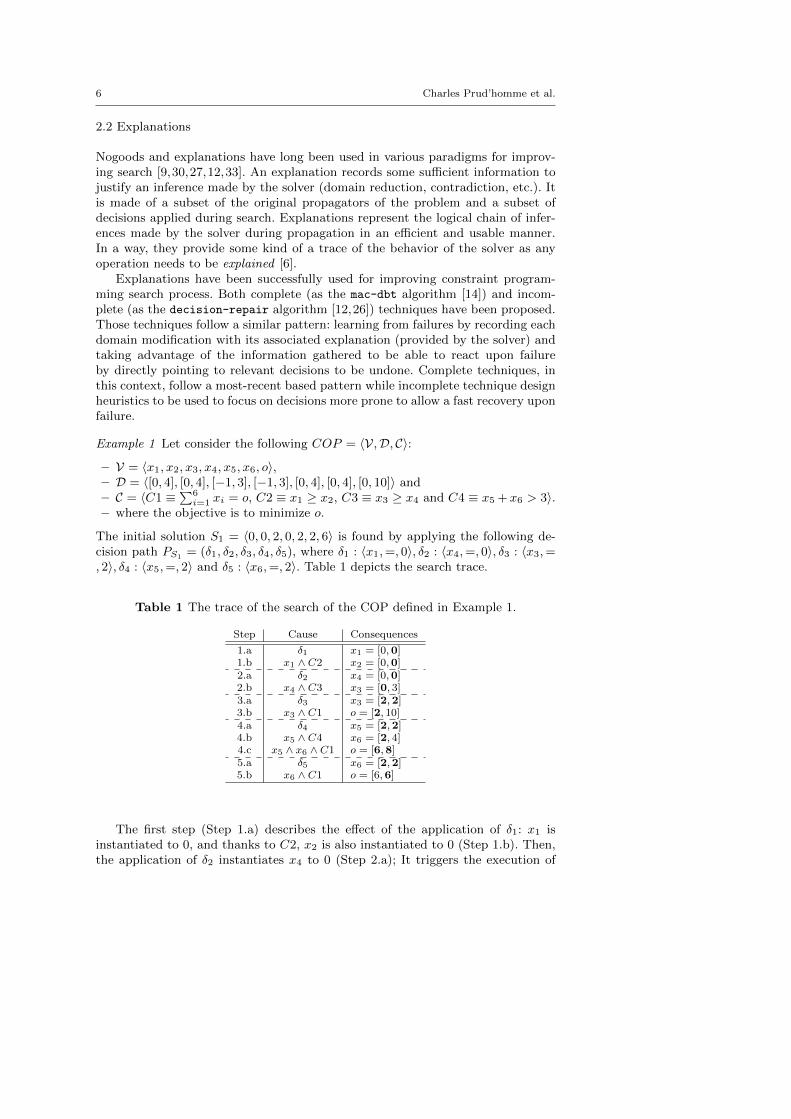
Table 1 The trace of the search of the COP defined in Example 1.
Step Cause Consequences
1.a δ1 x1 = [0,0]1.b x1 ∧ C2 x2 = [0,0]2.a δ2 x4 = [0,0]2.b x4 ∧ C3 x3 = [0, 3]3.a δ3 x3 = [2,2]3.b x3 ∧ C1 o = [2, 10]4.a δ4 x5 = [2,2]4.b x5 ∧ C4 x6 = [2, 4]4.c x5 ∧ x6 ∧ C1 o = [6,8]5.a δ5 x6 = [2,2]5.b x6 ∧ C1 o = [6,6]
The first step (Step 1.a) describes the effect of the application of δ1: x1 isinstantiated to 0, and thanks to C2, x2 is also instantiated to 0 (Step 1.b). Then,the application of δ2 instantiates x4 to 0 (Step 2.a); It triggers the execution of
Explanation-Based Large Neighborhood Search 7
the propagator of C3 which updates the lower bound of x3 to 0 (Step 2.b). Theapplication of δ3 instantiates x3 to 2 (Step 3.a), the lower bound of o is thenupdated to 2 because of C1 (Step 3.b). The application of δ4 instantiates x5 to2 (Step 4.a), it triggers the execution of the propagator of C4 which updates thelower bound of x6 to 2 (Step 4.b); Then, the update of the domain of o stemsfrom those two previous modifications (Step 4.c). Finally, the application of δ5instantiates x6 to 2 (Step 5.a). This events instantiates o to 6 by executing thepropagator of C1 (Step 5.b).
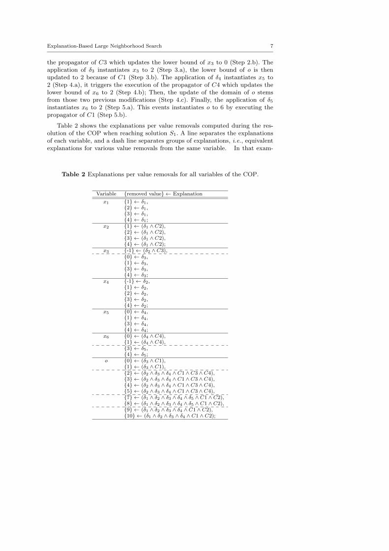
Table 2 shows the explanations per value removals computed during the res-olution of the COP when reaching solution S1. A line separates the explanationsof each variable, and a dash line separates groups of explanations, i.e., equivalentexplanations for various value removals from the same variable. In that exam-
Table 2 Explanations per value removals for all variables of the COP.
Variable {removed value} ← Explanation
x1 {1} ← δ1,{2} ← δ1,{3} ← δ1,{4} ← δ1;
x2 {1} ← (δ1 ∧ C2),{2} ← (δ1 ∧ C2),{3} ← (δ1 ∧ C2),{4} ← (δ1 ∧ C2);
x3 {-1} ← (δ2 ∧ C3),{0} ← δ3,{1} ← δ3,{3} ← δ3,{4} ← δ3;
x4 {-1} ← δ2,{1} ← δ2,{2} ← δ2,{3} ← δ2,{4} ← δ2;
x5 {0} ← δ4,{1} ← δ4,{3} ← δ4,{4} ← δ4;
x6 {0} ← (δ4 ∧ C4),{1} ← (δ4 ∧ C4),{3} ← δ5,{4} ← δ5;
o {0} ← (δ3 ∧ C1),{1} ← (δ3 ∧ C1),{2} ← (δ2 ∧ δ3 ∧ δ4 ∧ C1 ∧ C3 ∧ C4),{3} ← (δ2 ∧ δ3 ∧ δ4 ∧ C1 ∧ C3 ∧ C4),{4} ← (δ2 ∧ δ3 ∧ δ4 ∧ C1 ∧ C3 ∧ C4),{5} ← (δ2 ∧ δ3 ∧ δ4 ∧ C1 ∧ C3 ∧ C4),{7} ← (δ1 ∧ δ2 ∧ δ3 ∧ δ4 ∧ δ5 ∧ C1 ∧ C2),{8} ← (δ1 ∧ δ2 ∧ δ3 ∧ δ4 ∧ δ5 ∧ C1 ∧ C2),{9} ← (δ1 ∧ δ2 ∧ δ3 ∧ δ4 ∧ C1 ∧ C2),{10} ← (δ1 ∧ δ2 ∧ δ3 ∧ δ4 ∧ C1 ∧ C2);

8 Charles Prud’homme et al.
ple, some variables are uniformly explained, e.g., every value removal from x1 isexplained by δ1. That is also the case for x2, x4 and x5. Explanations may not beas obvious. Concerning o, all value removals are implied by propagation (e.g., 0is explained by δ3 ∧ C1), some of them are explained by a several decisions andconstraints. For instance, the explanation of the removal of 2 from o is not trivialto recover. Retrospectively, the increase of the lower bound of o is related to thesum constraint (C1) and the lower bounds of the variables involved, more preciselythe lower bounds of x3, x5 and x6. The lower bounds of x5 and x6 depends onthe application of δ4 through C4 and C1. The lower bound of x3 depends on theapplication of δ2, C3 and δ3. ♦
Key components of an explanation system. Adding explanations capabilities to aconstraint solver requires addressing several aspects:
– computing explanations: domain reductions are usually associated with a cause:the propagator that actually performed the modification. This information canbe used to compute an explanation. This can be done synchronously duringpropagation (by intrusive modification of the propagation algorithm) or asyn-chronously post propagation (by accessing an explanation service provided bypropagators).
– storing explanations: a data structure needs to be defined to be able to storedecisions made by the solver, domain reductions and their associated explana-tions. There exist several ways for storing explanations: a flattened storage ofthe domain modifications and their explanations composed of propagators andpreviously made decisions, or a unflattened storage of the domain modifica-tions and their explanations expressed through previous domain modifications[6]. The data structure is referred to as explanation store in the following.
– accessing explanations: the data structure used to store explanations needs toprovide access not only to domain modification explanations but also to currentupper and lower bounds of the domains, current domain as a whole, etc.
In [13], the authors give an overview of techniques used to compute explanationsand to handle them in a constraint solver. Despite being possibly very efficient,explanations suffer from several drawbacks:
– memory: storing explanations requires storing a way or another, variable mod-ifications;
– cpu: computing explanations usually comes with a cost even though the prop-agation algorithm can be partially used for that;
– software engineering: implementing explanations can be quite intrusive withina constraint solver.
Finally, explanations were initially designed to deal with satisfaction problems.Generally, an optimization problem is processed as a sequence of satisfaction prob-lems, in which cuts are added along with resolution to handle the optimizationcriterion. Regarding the explanation store, addition of cuts renders some explana-tions obsolete. Indeed, cuts cause modifications over domains that were previouslyachieved thanks to propagators.
Explanation-Based Large Neighborhood Search 9
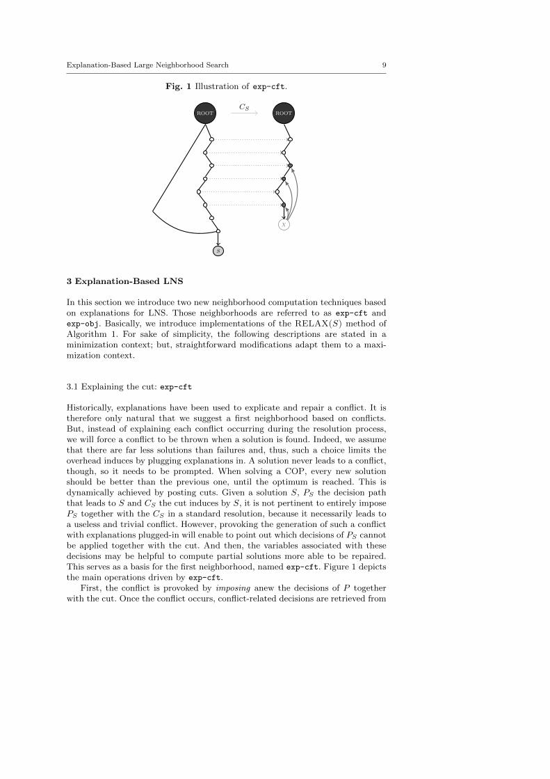
Fig. 1 Illustration of exp-cft.
ROOT
S
CSROOT
X
3 Explanation-Based LNS
In this section we introduce two new neighborhood computation techniques basedon explanations for LNS. Those neighborhoods are referred to as exp-cft andexp-obj. Basically, we introduce implementations of the RELAX(S) method ofAlgorithm 1. For sake of simplicity, the following descriptions are stated in aminimization context; but, straightforward modifications adapt them to a maxi-mization context.
3.1 Explaining the cut: exp-cft
Historically, explanations have been used to explicate and repair a conflict. It istherefore only natural that we suggest a first neighborhood based on conflicts.But, instead of explaining each conflict occurring during the resolution process,we will force a conflict to be thrown when a solution is found. Indeed, we assumethat there are far less solutions than failures and, thus, such a choice limits theoverhead induces by plugging explanations in. A solution never leads to a conflict,though, so it needs to be prompted. When solving a COP, every new solutionshould be better than the previous one, until the optimum is reached. This isdynamically achieved by posting cuts. Given a solution S, PS the decision paththat leads to S and CS the cut induces by S, it is not pertinent to entirely imposePS together with the CS in a standard resolution, because it necessarily leads toa useless and trivial conflict. However, provoking the generation of such a conflictwith explanations plugged-in will enable to point out which decisions of PS cannotbe applied together with the cut. And then, the variables associated with thesedecisions may be helpful to compute partial solutions more able to be repaired.This serves as a basis for the first neighborhood, named exp-cft. Figure 1 depictsthe main operations driven by exp-cft.
First, the conflict is provoked by imposing anew the decisions of P togetherwith the cut. Once the conflict occurs, conflict-related decisions are retrieved from
10 Charles Prud’homme et al.
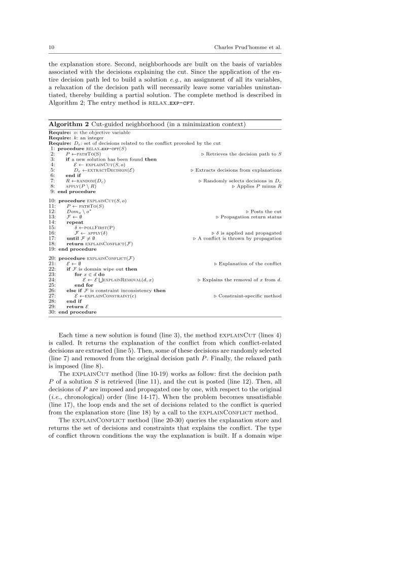
the explanation store. Second, neighborhoods are built on the basis of variablesassociated with the decisions explaining the cut. Since the application of the en-tire decision path led to build a solution e.g., an assignment of all its variables,a relaxation of the decision path will necessarily leave some variables uninstan-tiated, thereby building a partial solution. The complete method is described inAlgorithm 2; The entry method is relax exp-cft.
Algorithm 2 Cut-guided neighborhood (in a minimization context)Require: o: the objective variableRequire: k: an integerRequire: Dc: set of decisions related to the conflict provoked by the cut1: procedure relax exp-cft(S)2: P ←pathTo(S) . Retrieves the decision path to S3: if a new solution has been found then4: E ← explainCut(S, o)5: Dc ←extractDecision(E) . Extracts decisions from explanations6: end if7: R←random(Dc) . Randomly selects decisions in Dc
8: apply(P \ R) . Applies P minus R9: end procedure
10: procedure explainCut(S, o)11: P ← pathTo(S)12: Domo \ o∗ . Posts the cut13: F ← ∅ . Propagation return status14: repeat15: δ ←pollFirst(P)16: F ← apply(δ) . δ is applied and propagated17: until F 6= ∅ . A conflict is thrown by propagation18: return explainConflict(F)19: end procedure
20: procedure explainConflict(F)21: E ← ∅ . Explanation of the conflict22: if F is domain wipe out then23: for x ∈ d do24: E ← E
⋃explainRemoval(d, x) . Explains the removal of x from d.
25: end for26: else if F is constraint inconsistency then27: E ←explainConstraint(c) . Constraint-specific method28: end if29: return E30: end procedure
Each time a new solution is found (line 3), the method explainCut (lines 4)is called. It returns the explanation of the conflict from which conflict-relateddecisions are extracted (line 5). Then, some of these decisions are randomly selected(line 7) and removed from the original decision path P . Finally, the relaxed pathis imposed (line 8).
The explainCut method (line 10-19) works as follow: first the decision pathP of a solution S is retrieved (line 11), and the cut is posted (line 12). Then, alldecisions of P are imposed and propagated one by one, with respect to the original(i.e., chronological) order (line 14-17). When the problem becomes unsatisfiable(line 17), the loop ends and the set of decisions related to the conflict is queriedfrom the explanation store (line 18) by a call to the explainConflict method.
The explainConflict method (line 20-30) queries the explanation store andreturns the set of decisions and constraints that explains the conflict. The typeof conflict thrown conditions the way the explanation is built. If a domain wipe
Explanation-Based Large Neighborhood Search 11
out occurs (line 22), the resulting explanation is the conjunction of the explana-tion of each value removal (a call to the explainRemoval method, line 24). Ifa constraint inconstency is detected (line 26), the explainConstraint methodis called to retrieve an explanation (line 27). The default implementation callsthe explainRemoval method for all values removed from the variables of theconstraint; but constraint-specific implementations of the explainConstraintmethod provide more accurate explanations. At the end, both explainRemovaland explainConstraint query the explanation store .
Let Dc be the set of decisions related to the conflict provoked by the cut , thereare 2|Dc|−1 subsets of Dc, each of them corresponding to a possible relaxation ofP . Enumerating all the subsets of Dc is not polynomial, and there is no guaranteethat small neighborhoods are more able to build better solutions than bigger ones.Hence, to enforce the diversification of exp-cft and to test neighborhoods ofvarious sizes, we choose to randomly select α decisions to relax, where α is alsorandomly chosen in [1, |Dc| − 1].
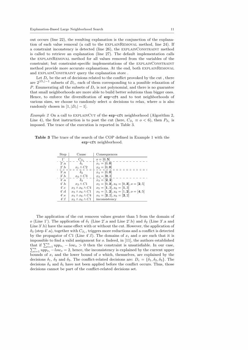
Example 2 On a call to explainCut of the exp-cft neighborhood (Algorithm 2,Line 4), the first instruction is to post the cut (here, CS1
≡ o < 6), then PS1is
imposed. The trace of the execution is reported in Table 3.
Table 3 The trace of the search of the COP defined in Example 1 with theexp-cft neighborhood.
Step Cause Consequences
1’ CS1o = [0,5]
2’.a δ1 x1 = [0,0]2’.b x1 ∧ C2 x2 = [0,0]
3’.a δ2 x4 = [0,0]3’.b x4 ∧ C3 x3 = [0, 3]4’.a δ3 x3 = [2,2]4’.b x3 ∧ C1 x5 = [0,3], x6 = [0,3], o = [2, 5]4’.c x5 ∧ x6 ∧ C4 x5 = [1, 3], x6 = [1, 3]4’.d x5 ∧ x6 ∧ C1 x5 = [1,2], x6 = [1,2], o = [4, 5]4’.e x5 ∧ x6 ∧ C4 x5 = [2, 2], x6 = [2, 2]4’.f x5 ∧ x6 ∧ C1 inconsistency
The application of the cut removes values greater than 5 from the domain ofo (Line 1’). The application of δ1 (Line 2’.a and Line 2’.b) and δ2 (Line 3’.a andLine 3’.b) have the same effect with or without the cut. However, the application ofδ3 (step 4’.a), together with CS1
, triggers more reductions and a conflict is detectedby the propagator of C1 (Line 4’.f). The domains of xi and o are such that it isimpossible to find a valid assignment for o. Indeed, in [11], the authors establishedthat if
∑ni=1 uppxi − lowo > 0 then the constraint is unsatisfiable. In our case,∑n
i=1 uppxi− lowo = 2, hence, the inconsistency is explained by the current upperbounds of xi and the lower bound of o which, themselves, are explained by thedecisions δ1, δ2 and δ3. The conflict-related decisions are: Dc = {δ1, δ2, δ3}. Thedecisions δ4 and δ5 have not been applied before the conflict occurs. Thus, thosedecisions cannot be part of the conflict-related decisions set.
12 Charles Prud’homme et al.
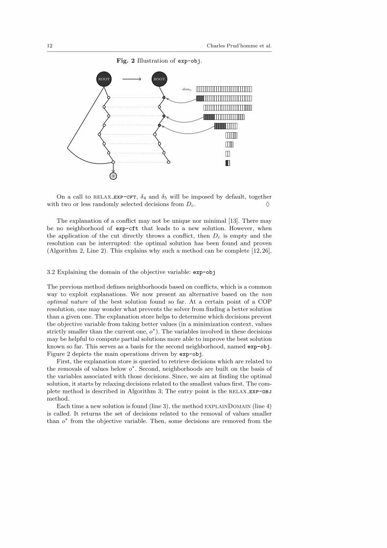
Fig. 2 Illustration of exp-obj.
ROOT
S
ROOT
domo
On a call to relax exp-cft, δ4 and δ5 will be imposed by default, togetherwith two or less randomly selected decisions from Dc. ♦
The explanation of a conflict may not be unique nor minimal [13]. There maybe no neighborhood of exp-cft that leads to a new solution. However, whenthe application of the cut directly throws a conflict, then Dc is empty and theresolution can be interrupted: the optimal solution has been found and proven(Algorithm 2, Line 2). This explains why such a method can be complete [12,26].
3.2 Explaining the domain of the objective variable: exp-obj
The previous method defines neighborhoods based on conflicts, which is a commonway to exploit explanations. We now present an alternative based on the nonoptimal nature of the best solution found so far. At a certain point of a COPresolution, one may wonder what prevents the solver from finding a better solutionthan a given one. The explanation store helps to determine which decisions preventthe objective variable from taking better values (in a minimization context, valuesstrictly smaller than the current one, o∗). The variables involved in these decisionsmay be helpful to compute partial solutions more able to improve the best solutionknown so far. This serves as a basis for the second neighborhood, named exp-obj.Figure 2 depicts the main operations driven by exp-obj.
First, the explanation store is queried to retrieve decisions which are related tothe removals of values below o∗. Second, neighborhoods are built on the basis ofthe variables associated with those decisions. Since, we aim at finding the optimalsolution, it starts by relaxing decisions related to the smallest values first. The com-plete method is described in Algorithm 3; The entry point is the relax exp-obj
method.Each time a new solution is found (line 3), the method explainDomain (line 4)
is called. It returns the set of decisions related to the removal of values smallerthan o∗ from the objective variable. Then, some decisions are removed from the
Explanation-Based Large Neighborhood Search 13
Algorithm 3 Domain-guided neighborhood (in a minimization context)Require: o: the objective variableRequire: k: an integerRequire: Dd: ordered set of decisions related to the domain of oRequire: I: array of integers1: procedure relax exp-obj(S)2: P ←pathTo(S) . Retrieves the decision path to S3: if a new solution has been found then4: explainDomain(S, o)5: k ← 06: end if7: k ← k + 18: R← ∅9: if k ≤ length(I) then
10: R←I[k]⋃j=1
Dd[j]
11: else12: R←random(Dd) . Randomly selects decisions in Dd
13: end if14: apply(P \ R) . Applies P minus R15: end procedure
16: procedure explainDomain(S, o)17: n← (o∗ − Lowo) . Gets the number of removed values18: Dd ← []; I ← [];19: for k ∈ [1, n] do20: E ← explainRemoval(do, Lowo + k − 1)21: Dd ← Dd
⋃extractDecision(E) . Queries the explanation store
22: I[k]← |Dd|23: end for24: end procedure
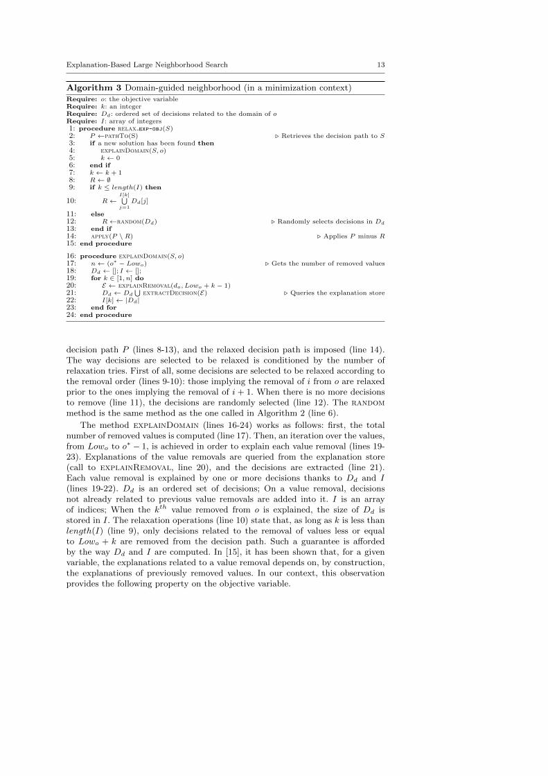
decision path P (lines 8-13), and the relaxed decision path is imposed (line 14).The way decisions are selected to be relaxed is conditioned by the number ofrelaxation tries. First of all, some decisions are selected to be relaxed according tothe removal order (lines 9-10): those implying the removal of i from o are relaxedprior to the ones implying the removal of i + 1. When there is no more decisionsto remove (line 11), the decisions are randomly selected (line 12). The randommethod is the same method as the one called in Algorithm 2 (line 6).
The method explainDomain (lines 16-24) works as follows: first, the totalnumber of removed values is computed (line 17). Then, an iteration over the values,from Lowo to o∗ − 1, is achieved in order to explain each value removal (lines 19-23). Explanations of the value removals are queried from the explanation store(call to explainRemoval, line 20), and the decisions are extracted (line 21).Each value removal is explained by one or more decisions thanks to Dd and I(lines 19-22). Dd is an ordered set of decisions; On a value removal, decisionsnot already related to previous value removals are added into it. I is an arrayof indices; When the kth value removed from o is explained, the size of Dd isstored in I. The relaxation operations (line 10) state that, as long as k is less thanlength(I) (line 9), only decisions related to the removal of values less or equalto Lowo + k are removed from the decision path. Such a guarantee is affordedby the way Dd and I are computed. In [15], it has been shown that, for a givenvariable, the explanations related to a value removal depends on, by construction,the explanations of previously removed values. In our context, this observationprovides the following property on the objective variable.
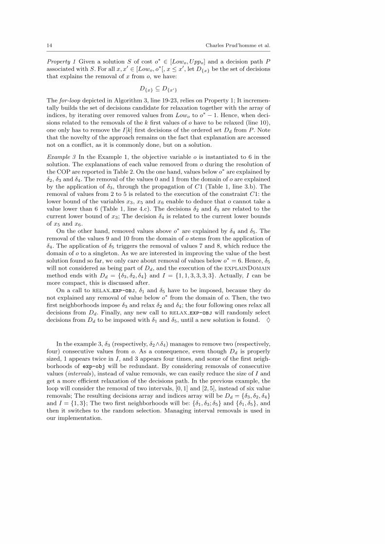
14 Charles Prud’homme et al.
Property 1 Given a solution S of cost o∗ ∈ [Lowo, Uppo] and a decision path Passociated with S. For all x, x′ ∈ [Lowo, o
∗[, x ≤ x′, let D{x} be the set of decisionsthat explains the removal of x from o, we have:
D{x} ⊆ D{x′}
The for-loop depicted in Algorithm 3, line 19-23, relies on Property 1; It incremen-tally builds the set of decisions candidate for relaxation together with the array ofindices, by iterating over removed values from Lowo to o∗ − 1. Hence, when deci-sions related to the removals of the k first values of o have to be relaxed (line 10),one only has to remove the I[k] first decisions of the ordered set Dd from P . Notethat the novelty of the approach remains on the fact that explanation are accessednot on a conflict, as it is commonly done, but on a solution.
Example 3 In the Example 1, the objective variable o is instantiated to 6 in thesolution. The explanations of each value removed from o during the resolution ofthe COP are reported in Table 2. On the one hand, values below o∗ are explained byδ2, δ3 and δ4. The removal of the values 0 and 1 from the domain of o are explainedby the application of δ3, through the propagation of C1 (Table 1, line 3.b). Theremoval of values from 2 to 5 is related to the execution of the constraint C1: thelower bound of the variables x3, x5 and x6 enable to deduce that o cannot take avalue lower than 6 (Table 1, line 4.c). The decisions δ2 and δ3 are related to thecurrent lower bound of x3; The decision δ4 is related to the current lower boundsof x5 and x6.
On the other hand, removed values above o∗ are explained by δ4 and δ5. Theremoval of the values 9 and 10 from the domain of o stems from the application ofδ4. The application of δ5 triggers the removal of values 7 and 8, which reduce thedomain of o to a singleton. As we are interested in improving the value of the bestsolution found so far, we only care about removal of values below o∗ = 6. Hence, δ5will not considered as being part of Dd, and the execution of the explainDomainmethod ends with Dd = {δ3, δ2, δ4} and I = {1, 1, 3, 3, 3, 3}. Actually, I can bemore compact, this is discussed after.
On a call to relax exp-obj, δ1 and δ5 have to be imposed, because they donot explained any removal of value below o∗ from the domain of o. Then, the twofirst neighborhoods impose δ3 and relax δ2 and δ4; the four following ones relax alldecisions from Dd. Finally, any new call to relax exp-obj will randomly selectdecisions from Dd to be imposed with δ1 and δ5, until a new solution is found. ♦
In the example 3, δ3 (respectively, δ2∧δ4) manages to remove two (respectively,four) consecutive values from o. As a consequence, even though Dd is properlysized, 1 appears twice in I, and 3 appears four times, and some of the first neigh-borhoods of exp-obj will be redundant. By considering removals of consecutivevalues (intervals), instead of value removals, we can easily reduce the size of I andget a more efficient relaxation of the decisions path. In the previous example, theloop will consider the removal of two intervals, [0, 1] and [2, 5], instead of six valueremovals; The resulting decisions array and indices array will be Dd = {δ3, δ2, δ4}and I = {1, 3}; The two first neighborhoods will be: {δ1, δ3; δ5} and {δ1, δ5}, andthen it switches to the random selection. Managing interval removals is used inour implementation.

Explanation-Based Large Neighborhood Search 15
These neighborhoods could be seen as an unnecessary complicated versionof the round-robin process in which one or more top-level decisions would bequestioned from the decision path. As shown in Example 3, not all (top-)decisionsare related to (lower) value removals from the objective variable, some of them donot question the quality of the best solution found so far. Moreover, the choice ofdecisions to relax is not made aimlessly and is directed by the objective variablethough explanations.
3.3 Additional information and further improvements
This section details the method to relax the decision path and techniques adoptedto improve the efficiency of the approaches described in this paper.
Relaxing the decision path. In this paragraph, we describe how the decision pathis effectively updated (Algorithm 2, line 7 and Algorithm 3, line 14). The methodapply(P \R) aims at removing a set of decisions R from a decision path P . First, alldecisions from R are removed from P . Then, negated decisions must be consideredtoo, even though they do not appear in R. Indeed, a decision δ is negated whenthe search process closes the sub-tree induced by δ, i.e., the entire sub-tree hasbeen explored. A decision which becomes negated is explained by higher decisionsin the search tree. So, if one decision which explains the negation of another one isremoved, then keeping the negated decision is not justified anymore, and it shouldbe removed too. For example, let P = {δ1, δ2, δ3,¬δ4} be a decision path andR = {δ2} be the set of decisions to remove from P ; The relaxed decision pathP ′ is equal to {δ1, δ3}. ¬δ4 is automatically removed because it is explained byδ1 ∧ δ2 ∧ δ3. More details about the explanation of negated decisions are givenin [13].
Lazy explanation recording. Conflict-based searches access to explanations on eachconflict [9,27,12]. Our approaches, on the contrary, only requires access on solu-tions. Consequently, it is not worth computing and storing explanations whilesolving. To avoid computing and storing useless information related to domain re-duction, we implement a lazy and asynchronous fashion way to compute and storedomain modifications, like described in [8]. Minimal data related to events gener-ated during the resolution (i.e., the variable, the modification and the cause) isstored into a queue all resolution long. This queue is backtrackable to store relevantinformation and to reduce non relevant one upon backtracking. When a solutionis found, the explanation store have to be queried, but is empty at that point.A computation routine is then executed: datas stored in the queue are poppedone by one (w.r.t. the chronological order), the explanations are computed andstored. Once the queue is empty, the explanation store is up to date and ready forqueries. Even though storing minimal data in the queue comes with a cost, it isnegligible in comparison with maintaining the explanation store during the searchand it significantly reduces both memory and cpu consumptions. Plugging lazyand asynchronous explanations in without querying the explanation store (norcomputing explanations) only slows down the resolution process by less than 10%.
16 Charles Prud’homme et al.
Explaining interval removals. Most of the time, domain reduction is treated as asequence of value removals. For instance, a lower bound modification from i tok− 1 is explained by the removal of all the values j from i to k− 1. Such behaviorbecomes pathological when variables have large domains, which is often the casefor the objective variable. Thus, it is mandatory to explain interval removals in-stead of value removals: it prevents from storing and computing a large amountof information and saves both and memory consumption. Our approach adaptsthe technique described in [15], originally proposed for numeric CSP, to integerdomains represented as intervals. Note that Lazy Clause Generation solvers handleinterval removals natively [32]. In LCG solvers, every value of the domain of aninteger variable is represented using boolean variables [[v = x]] and [[v ≤ x]]. Forinstance, the variable [[v = x]] is true if v takes the value x and false if v takes avalue different from x.
Dealing with enumerated domain objective variables. Generally, the objective vari-able is bounded, that is, its domain is an interval of integers. An alternative is todefine the domain as on ordered set of integers, the domain is said to be enumer-ated. Due to the size of the objective variable domain, which is generally very large,a bounded domain is often preferred to an enumerated one. In some cases, it isworth representing all values, though. Such a choice does not call into question thevalidity of the property 1 nor the behavior of exp-obj. But, it may build differentneighborhoods.
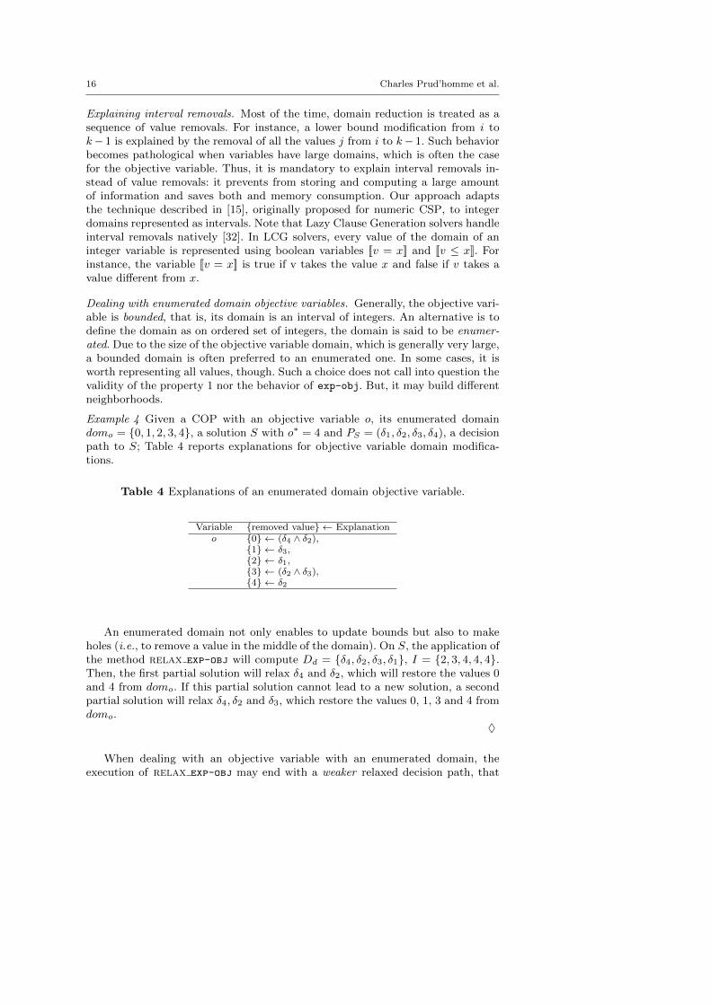
Example 4 Given a COP with an objective variable o, its enumerated domaindomo = {0, 1, 2, 3, 4}, a solution S with o∗ = 4 and PS = (δ1, δ2, δ3, δ4), a decisionpath to S; Table 4 reports explanations for objective variable domain modifica-tions.
Table 4 Explanations of an enumerated domain objective variable.
Variable {removed value} ← Explanationo {0} ← (δ4 ∧ δ2),
{1} ← δ3,{2} ← δ1,{3} ← (δ2 ∧ δ3),{4} ← δ2
An enumerated domain not only enables to update bounds but also to makeholes (i.e., to remove a value in the middle of the domain). On S, the application ofthe method relax exp-obj will compute Dd = {δ4, δ2, δ3, δ1}, I = {2, 3, 4, 4, 4}.Then, the first partial solution will relax δ4 and δ2, which will restore the values 0and 4 from domo. If this partial solution cannot lead to a new solution, a secondpartial solution will relax δ4, δ2 and δ3, which restore the values 0, 1, 3 and 4 fromdomo.
♦
When dealing with an objective variable with an enumerated domain, theexecution of relax exp-obj may end with a weaker relaxed decision path, that
Explanation-Based Large Neighborhood Search 17
is, values from o will be relaxed without necessarily respecting the lexical orderingof the domain.
Reconsidering the number of selected decisions. In Section 3.1, we explained howthe random selection of decisions to relax works: we select randomly α decisions torelax, where α is also randomly selected. However, the parameter α is not computedon each call to the random method, but every θ = minimum(
(|D|−1α
), 200) calls,
where D is either equal to Dc or Dd. This gives the opportunity to test a widerange of the possible combinations when
(|D|−1α
)is small enough, and to test only a
small subpart of them when the number is big. Various neighborhoods of the samesize are tested before a new value for α is picked. We evaluate other approaches,and this one brings more robustness and improves the overall resolution process.
4 Evaluation
The central objective of the exp-cft and exp-obj algorithms are to build betterneighborhoods in order to explore more appropriate parts of the search space andto speed up the LNS process. This section demonstrates the benefits of combiningexp-obj and exp-cft together.
4.1 Implementation of LNS
Propagation-Guided Large Neighborhood Search. Neither instance dependent butrelying on global parameters, this combination of three neighborhoods has beenproven to be very efficient on a modified version of the Car Sequencing Prob-lem [23]. On each call to the propagation-guided neighborhood (or pgn), a firstvariable is selected randomly to be part of the partial solution and is assignedto its value in the previous solution. This assignment is propagated through theconstraint network and the graph of dependencies is build: variables modified bypropagation are marked. Every marked variable not instantiated is then storedin priority list, where variables are sorted by the domain reduction that occurredon their domain. The top priority variable in the list is selected to be fixed. Theselection stops when the sum of the logarithm of the domain of all variables isbelow a given constant. The desired partial solution size is updated by adding amultiplicative correction factor epsilon. Two alternatives have been defined: Thereverse propagation-guided neighborhood (or repgn) is built by expansion insteadof by reduction; The random propagation-guided neighborhood (or rapgn) is im-plemented with a list of size 0. Hence, the first contender is made of a sequentialapplication of pgn, repgn and rapgn. We use the default parameters defined in [23]:the size of the list is set to 10, the constant is valued to 30 and the way epsilonevolves is dynamic. As we consider LNS as a black-box strategy here, we do nottry to adapt the parameters to the problem treated and we focus on the genericityof the approach. This contender is called PGLNS.
Explanation-Based LNS. We evaluate various combinations of the explanation-based neighborhoods presented in Section 3. The first combination is made ofexp-obj and a random neighborhood, named ran. The latter will have to bring
18 Charles Prud’homme et al.
diversification by providing neighborhoods which are not related to the problemstructure. Indeed, in [23], the authors “obtained better results by interleaving purelyrandom neighborhoods with more advanced ones”. Thus, ran relaxes ζ variablesrandomly selected on each call to the Relax method; the remaining ones areobviously instantiated to their value in the best solution known so far. ζ is set to|V|3 on a solution; and is incremented once every 200 calls to the neighborhood
computation. Such parameters enable a strong diversification. The first contenderis named objLNS. A second combination, named cftLNS, groups together exp-cftand ran. As exp-obj and exp-cft exploit explanations in two different ways, wesuggest a third combination, named EBLNS, made of exp-obj, exp-cft and ran.We hope EBLNS will improve the overall behavior of each neighborhood usedindividually.
In every contenders, each neighborhood is then applied fairly, in sequence, untila new solution is found.
Fast restarts. All contenders are evaluated with a fast restart strategy [22] pluggedin: we limit the reparation step to 30 fails. Such a strategy is commonly associatedwith LNS and has been proven to improve its efficiency.
Random LNS. A purely random neighborhood, made exclusively of ran, easy toimplement and configuration-free has been evaluated too. Due to its poor efficiencyin practice (it was never competitive with any other approaches evaluated here),the results are not reported here, though.2
4.2 Benchmark protocol
Propagation-Guided LNS and Explanation-Based LNS were implemented in Choco-3.1.0 [28], a Java library for constraint programming. All the experiments weredone on a Macbook Pro with a 6-core Intel Xeon at 2.93Ghz running on MacOS10.6.8, and Java 1.7. Each run had one core and a 15 minutes time limit. Dueto randomness, the evaluations were run ten times and the arithmetic mean ofthe objective value (obj), its range3 (rng) and the standard deviation (stddev) arereported. The range gives indication about the stability of an approach. Note thatthe first solution of each run of the same problem is always the same one, whateverversions of LNS is plugged in.
4.3 Benchmark description
The evaluation proposed here is based on ten problems composed of 49 instances.There are nine optimization problems extracted from the MiniZinc distributionand one additional problem, the Optimized Car Sequencing Problem.4 The latterone has been added to facilitate the comparison with PGLNS.
2 The complete results of purely random contender are available on request.3 The range: 100 ∗ highest−lowest
mean.
4 The Optimized Car Sequencing Problem (5 instances) is a modified version of the CarSequencing Problem in which an additional option-free configuration has been added (as de-scribed in [23]). The objective is to schedule the cars requiring this configuration at the end,in such a way that a solution to the original satisfaction problem is found.
Explanation-Based Large Neighborhood Search 19
We kept instances for which classic backtrack algorithm finds at least one solu-tion within a 15 minutes time limit: LNS needs an initial solution to be activated.
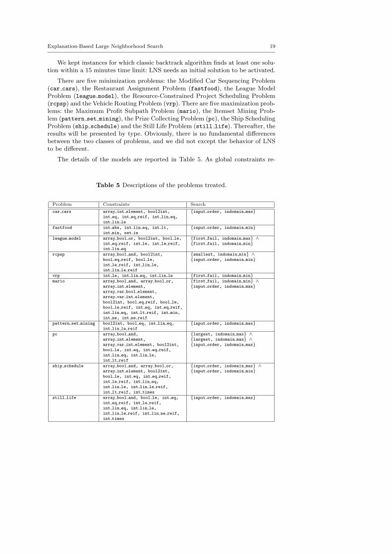
There are five minimization problems: the Modified Car Sequencing Problem(car cars), the Restaurant Assignment Problem (fastfood), the League ModelProblem (league model), the Resource-Constrained Project Scheduling Problem(rcpsp) and the Vehicle Routing Problem (vrp). There are five maximization prob-lems: the Maximum Profit Subpath Problem (mario), the Itemset Mining Prob-lem (pattern set mining), the Prize Collecting Problem (pc), the Ship SchedulingProblem (ship schedule) and the Still Life Problem (still life). Thereafter, theresults will be presented by type. Obviously, there is no fundamental differencesbetween the two classes of problems, and we did not except the behavior of LNSto be different.
The details of the models are reported in Table 5. As global constraints re-
Table 5 Descriptions of the problems treated.
Problem Constraints Search
car cars array int element, bool2int,int eq, int eq reif, int lin eq,int lin le
{input order, indomain max}
fastfood int abs, int lin eq, int lt,int min, set in
{input order, indomain min}
league model array bool or, bool2int, bool le,int eq reif, int le, int le reif,int lin eq
{first fail, indomain max} ∧{first fail, indomain min}
rcpsp array bool and, bool2int,bool eq reif, bool le,int le reif, int lin le,int lin le reif
{smallest, indomain min} ∧{input order, indomain min}
vrp int le, int lin eq, int lin le {first fail, indomain min}mario array bool and, array bool or,
array int element,array var bool element,array var int element,bool2int, bool eq reif, bool le,bool le reif, int eq, int eq reif,int lin eq, int lt reif, int min,int ne, int ne reif
{first fail, indomain min} ∧{input order, indomain max}
pattern set mining bool2int, bool eq, int lin eq,int lin le reif
{input order, indomain max}
pc array bool and,array int element,array var int element, bool2int,bool le, int eq, int eq reif,int lin eq, int lin le,int lt reif
{largest, indomain max} ∧{largest, indomain max} ∧{input order, indomain max}
ship schedule array bool and, array bool or,array int element, bool2int,bool le, int eq, int eq reif,int le reif, int lin eq,int lin le, int lin le reif,int lt reif, int times
{input order, indomain max} ∧{input order, indomain min}
still life array bool and, bool le, int eq,int eq reif, int le reif,int lin eq, int lin le,int lin le reif, int lin ne reif,int times
{input order, indomain max}
20 Charles Prud’homme et al.
quire implementation of specific explanation schemas, whose evaluation is not thepurpose of the paper, the problems are modeled with built-in constraints, whichare natively explained. The following problems were initially modeled with globalconstraints: the Modified Car Sequencing Problem, the League Model Problem,the Resource-Constrained Project Scheduling Problem, the Maximum Profit Sub-path Problem and the Itemset Mining Problem. Moreover, in half of the classes ofproblem, the search strategies are static: input order.
4.4 Evaluation of objLNS, cftLNS and EBLNS
The main motivation of this paper is twofold. First, we suggest two generic neigh-borhoods based on explanations for the LNS framework. They require neitheraccurate parameterization nor need to be adapted to the instance treated. Sec-ond, we show that they define neighborhoods more able to build new solutions,and thus improve the resolution of optimization problems. In this section, we com-pare various contenders based on explanations, objLNS, cftLNS and EBLNS, withthe propagation-guided one, PGLNS.
Various pairwise comparisons between contenders are done. The results arepresented in tables which report the arithmetic mean of the objective variable andits range of the approaches evaluated. Bold number highlights the best objectivevalue per instances; Italic numbers denote equality. We also use plots to displaythe multiplying factor over the objective value obtained by using one approachinstead of the other. The horizontal axis represents the instances treated, sortedwith respect of the difference between the solution found using the first approachh1 and the one using the second one h2, in increasing order. The vertical axisreports the multiplying factors, ρ(hi, hj) = max( hi
hj, 1). A mark on the left side of
the plot (light gray area) reports ρ(h1, h2) for an instance better solved with h1,it measures the loss of using h2 instead of h1. A mark on the right side of the plot(dark gray area) reports ρ(h2, h1) for an instance better solved with h2, it measuresthe gain of using h2 instead of h1. The plots also report the approximated areaA5 of the gain and loss. The larger the dark gray (respectively light gray) area is,the bigger the improvement (respectively, the loss) related to EBLNS.
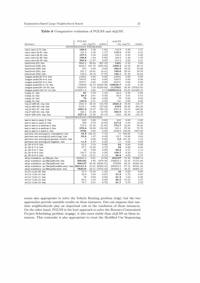
4.4.1 Comparative evaluation of PGLNS and objLNS
Table 6 reports the results obtained with PGLNS and objLNS on the ten problems.On 19 out of 49 instances, PGLNS is the best approach, whereas, on 26 instancesobjLNS is the more efficient. In about one-third of the cases (6 out of 9 for PGLNSand 8 out of 26 for objLNS) the range is almost 0. That means all resolutionstreated by the same contender lead to in the same last solution. Besides, there arefour instances where the two approaches are equivalent.
On the one hand, objLNS finds the best solutions for the Restaurant Assign-ment problem (fastfood), the League Model problem (league), the Prize Col-lecting problem (pc) and the Still Life problem (still life). objLNS is morestable than PGLNS on instances of the Restaurant Assignment problem and thePrize Collecting problem. That is not true for the other instances. This contender
5 The approximation is computed with the Trapezoidal rule [1].
Explanation-Based Large Neighborhood Search 21
Table 6 Comparative evaluation of PGLNS and objLNS.
PGLNS objLNSInstance obj rng(%) stddev obj rng(%) stddev
MINIMIZATION PROBLEMScars cars 4 72.fzn 109.3 5.49 1.85 116.9 4.28 1.51cars cars 16 81.fzn 121.2 2.48 1.17 119.5 6.69 3.41cars cars 26 82.fzn 127.5 5.49 2.20 136.6 6.59 2.29cars cars 41 66.fzn 108.8 1.84 0.98 109.8 5.46 1.40cars cars 90 05.fzn 300.8 11.97 9.93 319.3 2.82 3.41fastfood ff3.fzn 3883.4 90.64 967.10 1331 0.45 2.05fastfood ff58.fzn 8882.7 101.78 2955.56 1399.2 10.58 46.12fastfood ff59.fzn 871 0.00 0.00 294.6 32.59 25.00fastfood ff61.fzn 221.7 24.81 16.41 189.6 29.54 16.50fastfood ff63.fzn 146.9 40.16 17.70 120.1 47.46 16.69league model20-3-5.fzn 49984 0.00 0.00 49984 0.00 0.00league model30-4-6.fzn 79973 0.00 0.00 79973 0.00 0.00league model50-4-4.fzn 99971 0.00 0.00 99971 0.00 0.00league model55-3-12.fzn 139949 35.73 18439.09 109949.7 0.00 0.46league model90-18-20.fzn 1922916 7.28 35228.00 1117921 39.36 137823.82league model100-21-12.fzn 3139911.9 0.00 2.17 2486918.6 85.65 818388.45rcpsp 11.fzn 81 3.70 1.10 83.6 2.39 0.66rcpsp 12.fzn 38.3 2.61 0.46 39.9 5.01 0.54rcpsp 13.fzn 78 0.00 0.00 79 0.00 0.00rcpsp 14.fzn 140.9 0.71 0.30 141 0.00 0.00vrp A-n38-k5.vrp.fzn 2341.6 22.16 155.59 2322.2 18.30 116.17vrp A-n62-k8.vrp.fzn 6318.1 6.66 127.92 6104 29.26 454.38vrp B-n51-k7.vrp.fzn 4291.8 15.87 189.12 4355.8 19.74 246.86vrp P-n20-k2.vrp.fzn 402.1 41.28 43.70 358.9 21.73 22.50vrp P-n60-k15.vrp.fzn 2271.9 12.28 91.15 2424 20.30 135.45
MAXIMIZATION PROBLEMSmario mario easy 2.fzn 628 0.00 0.00 628 0.00 0.00mario mario easy 4.fzn 506 8.70 13.05 517.6 8.50 19.05mario mario n medium 2.fzn 719.9 31.95 61.85 774.7 22.85 59.38mario mario n medium 4.fzn 576.6 52.90 110.30 555.1 37.29 72.76mario mario t hard 1.fzn 4783 0.00 0.00 3199.9 148.00 1947.09pattern set mining k1 ionosphere.fzn 16.9 130.18 7.12 11 100.00 3.46pattern set mining k2 audiology.fzn 53.6 1.87 0.49 52.7 18.98 3.03pattern set mining k2 german-credit.fzn 3 0.00 0.00 3.8 131.58 1.54pattern set mining k2 segment.fzn 11.8 8.47 0.40 11 0.00 0.00pc 25-5-5-9.fzn 62.8 3.18 0.98 64 0.00 0.00pc 28-4-7-4.fzn 47.7 12.58 2.72 58 0.00 0.00pc 30-5-6-7.fzn 60 0.00 0.00 60.9 6.57 1.14pc 32-4-8-0.fzn 104.7 14.33 4.38 109.7 8.20 3.41pc 32-4-8-2.fzn 84.9 15.31 6.14 89.8 6.68 2.75ship-schedule.cp 5Ships.fzn 483645.5 0.01 13.50 452157 19.40 37368.74ship-schedule.cp 6ShipsMixed.fzn 300185 4.86 4378.36 248822.5 43.45 41741.68ship-schedule.cp 7ShipsMixed.fzn 396137 20.40 23645.31 279396 89.34 84364.24ship-schedule.cp 7ShipsMixedUnconst.fzn 364141.5 21.01 26324.16 285652.5 87.13 80181.40ship-schedule.cp 8ShipsUnconst.fzn 782516 20.51 53704.49 584308.5 48.27 89265.47still-life 09.fzn 37.6 13.30 1.50 42 0.00 0.00still-life 10.fzn 49.8 4.02 0.87 51.9 5.78 0.94still-life 11.fzn 59 0.00 0.00 61.3 1.63 0.46still-life 12.fzn 63.3 4.74 0.90 66.5 21.05 4.57still-life 13.fzn 79.7 2.51 0.78 81.7 9.79 2.79
seems also appropriate to solve the Vehicle Routing problem (vrp), but the twoapproaches provide unstable results on these instances. One can suppose that ran-dom neighborhoods play an important role in the resolution of those instances.On the other hand, PGLNS is the best approach to solve the Resouce-ConstrainedProject Scheduling problem (rcpsp), it also more stable than objLNS on these in-stances. This contender is also appropriate to treat the Modified Car Sequencing
22 Charles Prud’homme et al.
problem (car cars), the Itemset Mining problem (pattern set mining) and theShip Scheduling problem (ship schedule), where it is also more stable. More gen-erally, PGLNS is more stable (16.4%), in average, than objLNS (24.54%).
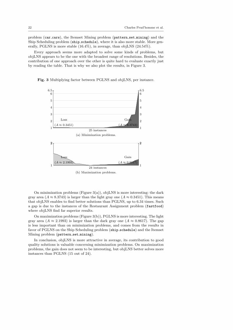
Every approach seems more adapted to solve some kinds of problems, butobjLNS appears to be the one with the broadest range of resolutions. Besides, thecontribution of one approach over the other is quite hard to evaluate exactly justby reading the table. That is why we also plot the results, in Figure 3.
Fig. 3 Multiplying factor between PGLNS and objLNS, per instance.
1 1
6.5 6.5
2 2
3 3
4 4
5 5
6 6
25 instances
(A ≈ 0.3451)
Loss
(A ≈ 8.3743)
Gain
(a) Minimization problems.
1 1
2 22 2
24 instances
(A ≈ 2.1993)
Loss
(A ≈ 0.8617)
Gain
(b) Maximization problems.
On minimization problems (Figure 3(a)), objLNS is more interesting: the darkgray area (A ≈ 8.3743) is larger than the light gray one (A ≈ 0.3451). This meansthat objLNS enables to find better solutions than PGLNS, up to 6.34 times. Sucha gap is due to the instances of the Restaurant Assignment problem (fastfood)where objLNS find far superior results.
On maximization problems (Figure 3(b)), PGLNS is more interesting. The lightgray area (A ≈ 2.1993) is larger than the dark gray one (A ≈ 0.8617). The gapis less important than on minimization problems, and comes from the results infavor of PGLNS on the Ship Scheduling problem (ship schedule) and the ItemsetMining problem (pattern set mining).
In conclusion, objLNS is more attractive in average, its contribution to goodquality solutions is valuable concerning minimization problems. On maximizationproblems, the gain does not seem to be interesting, but objLNS better solves moreinstances than PGLNS (15 out of 24).

Explanation-Based Large Neighborhood Search 23
4.4.2 Comparative evaluation of PGLNS and cftLNS
Table 7 reports results obtained with PGLNS and cftLNS on the 49 instances.In comparison with PGLNS, cftLNS better treats 29 out of 49 instances, whereas
Table 7 Comparative evaluation of PGLNS and cftLNS.
PGLNS cftLNSInstance obj rng(%) stddev obj rng(%) stddev
MINIMIZATION PROBLEMScars cars 4 72.fzn 109.3 5.49 1.85 117.1 4.27 1.51cars cars 16 81.fzn 121.2 2.48 1.17 119.9 6.67 3.30cars cars 26 82.fzn 127.5 5.49 2.20 136.8 5.85 2.64cars cars 41 66.fzn 108.8 1.84 0.98 109.8 5.46 1.40cars cars 90 05.fzn 300.8 11.97 9.93 319.5 2.50 3.01fastfood ff3.fzn 3883.4 90.64 967.10 1330 0.00 0.00fastfood ff58.fzn 8882.7 101.78 2955.56 1329.2 16.48 87.60fastfood ff59.fzn 871 0.00 0.00 279.6 16.81 18.80fastfood ff61.fzn 221.7 24.81 16.41 157.2 18.45 10.49fastfood ff63.fzn 146.9 40.16 17.70 103.9 0.96 0.30league model20-3-5.fzn 49984 0.00 0.00 49984 0.00 0.00league model30-4-6.fzn 79973 0.00 0.00 79973 0.00 0.00league model50-4-4.fzn 99971 0.00 0.00 99971 0.00 0.00league model55-3-12.fzn 139949 35.73 18439.09 109949.9 0.00 0.30league model90-18-20.fzn 1922916 7.28 35228.00 1730925.5 26.58 132319.46league model100-21-12.fzn 3139911.9 0.00 2.17 3103922.1 2.58 23747.70rcpsp 11.fzn 81 3.70 1.10 81.9 1.22 0.30rcpsp 12.fzn 38.3 2.61 0.46 39.3 5.09 0.64rcpsp 13.fzn 78 0.00 0.00 78 0.00 0.00rcpsp 14.fzn 140.9 0.71 0.30 141 0.00 0.00vrp A-n38-k5.vrp.fzn 2341.6 22.16 155.59 2106.2 44.44 261.66vrp A-n62-k8.vrp.fzn 6318.1 6.66 127.92 6117.2 16.30 310.67vrp B-n51-k7.vrp.fzn 4291.8 15.87 189.12 4019.1 29.83 353.93vrp P-n20-k2.vrp.fzn 402.1 41.28 43.70 336.8 23.46 26.14vrp P-n60-k15.vrp.fzn 2271.9 12.28 91.15 2317.8 29.99 224.26
MAXIMIZATION PROBLEMSmario mario easy 2.fzn 628 0.00 0.00 628 0.00 0.00mario mario easy 4.fzn 506 8.70 13.05 510.1 8.63 17.47mario mario n medium 2.fzn 719.9 31.95 61.85 889 25.20 63.14mario mario n medium 4.fzn 576.6 52.90 110.30 723.9 28.60 74.47mario mario t hard 1.fzn 4783 0.00 0.00 3039.4 157.37 1679.16pattern set mining k1 ionosphere.fzn 16.9 130.18 7.12 26.6 150.38 15.94pattern set mining k2 audiology.fzn 53.6 1.87 0.49 54 0.00 0.00pattern set mining k2 german-credit.fzn 3 0.00 0.00 4.9 81.63 1.30pattern set mining k2 segment.fzn 11.8 8.47 0.40 11 0.00 0.00pc 25-5-5-9.fzn 62.8 3.18 0.98 64.2 1.56 0.40pc 28-4-7-4.fzn 47.7 12.58 2.72 57.2 13.99 2.40pc 30-5-6-7.fzn 60 0.00 0.00 62.7 6.38 1.62pc 32-4-8-0.fzn 104.7 14.33 4.38 111.2 8.09 3.60pc 32-4-8-2.fzn 84.9 15.31 6.14 91.6 4.37 1.20ship-schedule.cp 5Ships.fzn 483645.5 0.01 13.50 483602.5 0.02 47.50ship-schedule.cp 6ShipsMixed.fzn 300185 4.86 4378.36 251359.5 68.71 63750.63ship-schedule.cp 7ShipsMixed.fzn 396137 20.40 23645.31 302325.5 10.34 10123.47ship-schedule.cp 7ShipsMixedUnconst.fzn 364141.5 21.01 26324.16 318492.5 23.42 27619.44ship-schedule.cp 8ShipsUnconst.fzn 782516 20.51 53704.49 470266.5 22.39 31509.21still-life 09.fzn 37.6 13.30 1.50 42 0.00 0.00still-life 10.fzn 49.8 4.02 0.87 53.6 3.73 0.66still-life 11.fzn 59 0.00 0.00 61.2 1.63 0.40still-life 12.fzn 63.3 4.74 0.90 75.1 2.66 0.54still-life 13.fzn 79.7 2.51 0.78 87.2 3.44 0.87
PGLNS is the most efficient on 15 cases. There are 6 equalities. In about one-third
24 Charles Prud’homme et al.
of the cases (5 out of 15 for PGLNS, 8 out of 29 for cftLNS), the range is equal to0, which indicates a good stability of the approaches.
The distribution is very similar to the one observed with objLNS: cftLNS issuitable for the Restaurant Assignment problem (fastfood), the League Modelproblem (league), the Prize Collecting problem (pc) and the Still Life problem(still life). cftLNS does not bring more stability in comparison with objLNS,though. Besides, cftLNS seems to be appropriate to deal with the Vehicle Rout-ing problem (vrp), the Maximum Profit Subpath (mario) and the Itemset Miningproblem (pattern set mining) with respect to PGLNS. But, it is less obviousto conclude regarding its stability. We observe larger gaps, in particular on in-stances of the Itemset Mining problem (pattern set mining). PGLNS remainsthe best approach to solve efficiently instances of the Ship Scheduling problem(ship schedule) and the Modified Car Sequencing problem (car cars). On thislast problem, one may see that one instance is better solved with cftLNS. In gen-eral, PGLNS is a little more stable than cftLNS (16.4% for PGLNS, 17.94% forcftLNS).
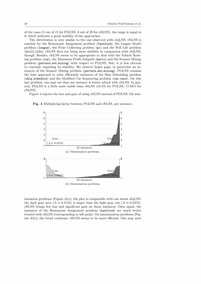
Figure 4 reports the loss and gain of using cftLNS instead of PGLNS. On min-
Fig. 4 Multiplying factor between PGLNS and cftLNS, per instance.
1 1
7 7
2 2
3 3
4 4
5 5
6 6
7 7
25 instances
(A ≈ 0.2373)
Loss
(A ≈ 8.5131)
Gain
(a) Minimization problems.
1 1
2 22 2
24 instances
(A ≈ 1.6263)
Loss
(A ≈ 2.3151)
Gain
(b) Maximization problems.
imization problems (Figure 4(a)), the plot is comparable with one about objLNS:the dark gray area (A ≈ 8.5131) is larger than the light gray one (A ≈ 0.2373).cftLNS brings few loss and significant gain on those instances. Once again, theinstances of the Restaurant Assignment problem (fastfood) are much bettertreated with cftLNS (corresponding to left peak). On maximization problems (Fig-ure 4(b)), the trend continues: cftLNS seems to be more efficient. One may note
Explanation-Based Large Neighborhood Search 25
that not only the dark gray area (A ≈ 2.31.51) is larger than the light gray one(A ≈ 1.6263), which means that cftLNS builds better quality solutions in average,but also that it betters more instances (16 out 24 for cftLNS, 7 for PGLNS).
In conclusion, cftLNS appears to be a good alternative to PGLNS, not only interm of the number of instances better solved, but also in term of gain regardingthe neighborhoods guided by propagation.
4.4.3 Comparative evaluation of objLNS and cftLNS
Results of cftLNS and objLNS seem to be very similar, in comparison with PGLNS.Now, we compare these two approaches and report the results in the Table 8. ThecftLNS approach dominates: it betters 28 out of 49 instances, whereas objLNSfinds better solution in 13 cases. There are eight equalities. In addition, cftLNS ismore stable in average (17.94% for cftLNS, 24.54% for objLNS). objLNS is the bestapproach to solve instances of the Modified Car Sequencing problem (car cars)and the League Model problem (league model), though. Regarding cftLNS, it ismore suitable to solve instances of the Restaurant Assignment problem (fastfood),the Resource-Constrained Project Scheduling problem (rcpsp), and, even less so,the Vehicle Routing problem (vrp), the Itemset Mining (pattern set mining) andthe Still Life problem (still life). Only a few instances of the Maximum ProfitSubpath problem (mario) are hard to decide between the two contenders.
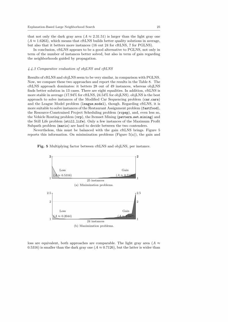
Nevertheless, this must be balanced with the gain cftLNS brings. Figure 5reports this information. On minimization problems (Figure 5(a)), the gain and
Fig. 5 Multiplying factor between cftLNS and objLNS, per instance.
1 1
2 22 2
25 instances
(A ≈ 0.5316)
Loss
(A ≈ 0.7126)
Gain
(a) Minimization problems.
1 1
2.5 2.5
2 2
24 instances
(A ≈ 0.2044)
Loss
(A ≈ 2.047)
Gain
(b) Maximization problems.
loss are equivalent, both approaches are comparable. The light gray area (A ≈0.5316) is smaller than the dark gray one (A ≈ 0.7126), but the latter is wider than

26 Charles Prud’homme et al.
Table 8 Comparative evaluation of objLNS and cftLNS.
objLNS cftLNSInstance obj rng(%) stddev obj rng(%) stddev
Problmes de minimisationcars cars 4 72.fzn 116.9 4.28 1.51 117.1 4.27 1.51cars cars 16 81.fzn 119.5 6.69 3.41 119.9 6.67 3.30cars cars 26 82.fzn 136.6 6.59 2.29 136.8 5.85 2.64cars cars 41 66.fzn 109.8 5.46 1.40 109.8 5.46 1.40cars cars 90 05.fzn 319.3 2.82 3.41 319.5 2.50 3.01fastfood ff3.fzn 1331 0.45 2.05 1330 0.00 0.00fastfood ff58.fzn 1399.2 10.58 46.12 1329.2 16.48 87.60fastfood ff59.fzn 294.6 32.59 25.00 279.6 16.81 18.80fastfood ff61.fzn 189.6 29.54 16.50 157.2 18.45 10.49fastfood ff63.fzn 120.1 47.46 16.69 103.9 0.96 0.30league model20-3-5.fzn 49984 0.00 0.00 49984 0.00 0.00league model30-4-6.fzn 79973 0.00 0.00 79973 0.00 0.00league model50-4-4.fzn 99971 0.00 0.00 99971 0.00 0.00league model55-3-12.fzn 109949.7 0.00 0.46 109949.9 0.00 0.30league model90-18-20.fzn 1117921 39.36 137823.82 1730925.5 26.58 132319.46league model100-21-12.fzn 2486918.6 85.65 818388.45 3103922.1 2.58 23747.70rcpsp 11.fzn 83.6 2.39 0.66 81.9 1.22 0.30rcpsp 12.fzn 39.9 5.01 0.54 39.3 5.09 0.64rcpsp 13.fzn 79 0.00 0.00 78 0.00 0.00rcpsp 14.fzn 141 0.00 0.00 141 0.00 0.00vrp A-n38-k5.vrp.fzn 2322.2 18.30 116.17 2106.2 44.44 261.66vrp A-n62-k8.vrp.fzn 6104 29.26 454.38 6117.2 16.30 310.67vrp B-n51-k7.vrp.fzn 4355.8 19.74 246.86 4019.1 29.83 353.93vrp P-n20-k2.vrp.fzn 358.9 21.73 22.50 336.8 23.46 26.14vrp P-n60-k15.vrp.fzn 2424 20.30 135.45 2317.8 29.99 224.26
Problmes de maximisationmario mario easy 2.fzn 628 0.00 0.00 628 0.00 0.00mario mario easy 4.fzn 517.6 8.50 19.05 510.1 8.63 17.47mario mario n medium 2.fzn 774.7 22.85 59.38 889 25.20 63.14mario mario n medium 4.fzn 555.1 37.29 72.76 723.9 28.60 74.47mario mario t hard 1.fzn 3199.9 148.00 1947.09 3039.4 157.37 1679.16pattern set mining k1 ionosphere.fzn 11 100.00 3.46 26.6 150.38 15.94pattern set mining k2 audiology.fzn 52.7 18.98 3.03 54 0.00 0.00pattern set mining k2 german-credit.fzn 3.8 131.58 1.54 4.9 81.63 1.30pattern set mining k2 segment.fzn 11 0.00 0.00 11 0.00 0.00pc 25-5-5-9.fzn 64 0.00 0.00 64.2 1.56 0.40pc 28-4-7-4.fzn 58 0.00 0.00 57.2 13.99 2.40pc 30-5-6-7.fzn 60.9 6.57 1.14 62.7 6.38 1.62pc 32-4-8-0.fzn 109.7 8.20 3.41 111.2 8.09 3.60pc 32-4-8-2.fzn 89.8 6.68 2.75 91.6 4.37 1.20ship-schedule.cp 5Ships.fzn 452157 19.40 37368.74 483602.5 0.02 47.50ship-schedule.cp 6ShipsMixed.fzn 248822.5 43.45 41741.68 251359.5 68.71 63750.63ship-schedule.cp 7ShipsMixed.fzn 279396 89.34 84364.24 302325.5 10.34 10123.47ship-schedule.cp 7ShipsMixedUnconst.fzn 285652.5 87.13 80181.40 318492.5 23.42 27619.44ship-schedule.cp 8ShipsUnconst.fzn 584308.5 48.27 89265.47 470266.5 22.39 31509.21still-life 09.fzn 42 0.00 0.00 42 0.00 0.00still-life 10.fzn 51.9 5.78 0.94 53.6 3.73 0.66still-life 11.fzn 61.3 1.63 0.46 61.2 1.63 0.40still-life 12.fzn 66.5 21.05 4.57 75.1 2.66 0.54still-life 13.fzn 81.7 9.79 2.79 87.2 3.44 0.87
it is tall. This confirms that cftLNS better solves more instances than objLNS butthat the gain is low. By contrast, objLNS brings more gain but on fewer instances.On maximization problems (Figure 5(b)), the results are clearly in favor of cftLNS.
Explanation-Based Large Neighborhood Search 27
4.4.4 Comparative evaluation of EBLNS and PGLNS
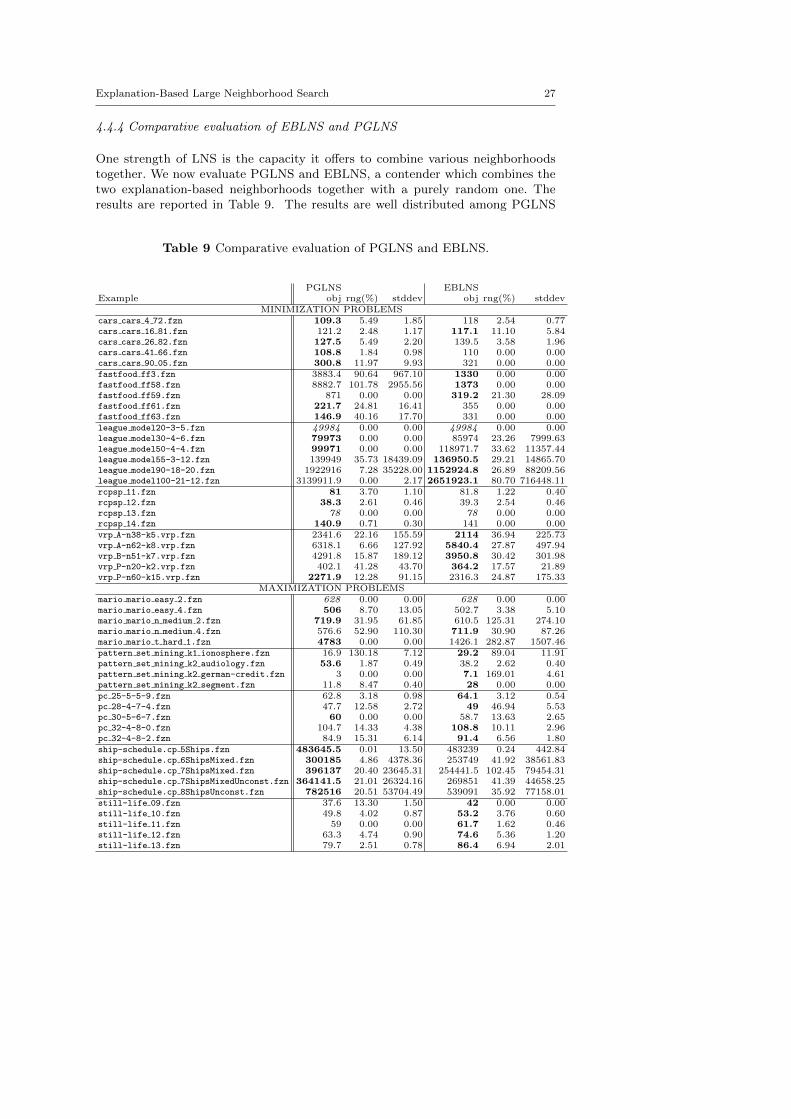
One strength of LNS is the capacity it offers to combine various neighborhoodstogether. We now evaluate PGLNS and EBLNS, a contender which combines thetwo explanation-based neighborhoods together with a purely random one. Theresults are reported in Table 9. The results are well distributed among PGLNS
Table 9 Comparative evaluation of PGLNS and EBLNS.
PGLNS EBLNSExample obj rng(%) stddev obj rng(%) stddev
MINIMIZATION PROBLEMScars cars 4 72.fzn 109.3 5.49 1.85 118 2.54 0.77cars cars 16 81.fzn 121.2 2.48 1.17 117.1 11.10 5.84cars cars 26 82.fzn 127.5 5.49 2.20 139.5 3.58 1.96cars cars 41 66.fzn 108.8 1.84 0.98 110 0.00 0.00cars cars 90 05.fzn 300.8 11.97 9.93 321 0.00 0.00fastfood ff3.fzn 3883.4 90.64 967.10 1330 0.00 0.00fastfood ff58.fzn 8882.7 101.78 2955.56 1373 0.00 0.00fastfood ff59.fzn 871 0.00 0.00 319.2 21.30 28.09fastfood ff61.fzn 221.7 24.81 16.41 355 0.00 0.00fastfood ff63.fzn 146.9 40.16 17.70 331 0.00 0.00league model20-3-5.fzn 49984 0.00 0.00 49984 0.00 0.00league model30-4-6.fzn 79973 0.00 0.00 85974 23.26 7999.63league model50-4-4.fzn 99971 0.00 0.00 118971.7 33.62 11357.44league model55-3-12.fzn 139949 35.73 18439.09 136950.5 29.21 14865.70league model90-18-20.fzn 1922916 7.28 35228.00 1152924.8 26.89 88209.56league model100-21-12.fzn 3139911.9 0.00 2.17 2651923.1 80.70 716448.11rcpsp 11.fzn 81 3.70 1.10 81.8 1.22 0.40rcpsp 12.fzn 38.3 2.61 0.46 39.3 2.54 0.46rcpsp 13.fzn 78 0.00 0.00 78 0.00 0.00rcpsp 14.fzn 140.9 0.71 0.30 141 0.00 0.00vrp A-n38-k5.vrp.fzn 2341.6 22.16 155.59 2114 36.94 225.73vrp A-n62-k8.vrp.fzn 6318.1 6.66 127.92 5840.4 27.87 497.94vrp B-n51-k7.vrp.fzn 4291.8 15.87 189.12 3950.8 30.42 301.98vrp P-n20-k2.vrp.fzn 402.1 41.28 43.70 364.2 17.57 21.89vrp P-n60-k15.vrp.fzn 2271.9 12.28 91.15 2316.3 24.87 175.33
MAXIMIZATION PROBLEMSmario mario easy 2.fzn 628 0.00 0.00 628 0.00 0.00mario mario easy 4.fzn 506 8.70 13.05 502.7 3.38 5.10mario mario n medium 2.fzn 719.9 31.95 61.85 610.5 125.31 274.10mario mario n medium 4.fzn 576.6 52.90 110.30 711.9 30.90 87.26mario mario t hard 1.fzn 4783 0.00 0.00 1426.1 282.87 1507.46pattern set mining k1 ionosphere.fzn 16.9 130.18 7.12 29.2 89.04 11.91pattern set mining k2 audiology.fzn 53.6 1.87 0.49 38.2 2.62 0.40pattern set mining k2 german-credit.fzn 3 0.00 0.00 7.1 169.01 4.61pattern set mining k2 segment.fzn 11.8 8.47 0.40 28 0.00 0.00pc 25-5-5-9.fzn 62.8 3.18 0.98 64.1 3.12 0.54pc 28-4-7-4.fzn 47.7 12.58 2.72 49 46.94 5.53pc 30-5-6-7.fzn 60 0.00 0.00 58.7 13.63 2.65pc 32-4-8-0.fzn 104.7 14.33 4.38 108.8 10.11 2.96pc 32-4-8-2.fzn 84.9 15.31 6.14 91.4 6.56 1.80ship-schedule.cp 5Ships.fzn 483645.5 0.01 13.50 483239 0.24 442.84ship-schedule.cp 6ShipsMixed.fzn 300185 4.86 4378.36 253749 41.92 38561.83ship-schedule.cp 7ShipsMixed.fzn 396137 20.40 23645.31 254441.5 102.45 79454.31ship-schedule.cp 7ShipsMixedUnconst.fzn 364141.5 21.01 26324.16 269851 41.39 44658.25ship-schedule.cp 8ShipsUnconst.fzn 782516 20.51 53704.49 539091 35.92 77158.01still-life 09.fzn 37.6 13.30 1.50 42 0.00 0.00still-life 10.fzn 49.8 4.02 0.87 53.2 3.76 0.60still-life 11.fzn 59 0.00 0.00 61.7 1.62 0.46still-life 12.fzn 63.3 4.74 0.90 74.6 5.36 1.20still-life 13.fzn 79.7 2.51 0.78 86.4 6.94 2.01
28 Charles Prud’homme et al.
and EBLNS: in 22 out of 49 examples, PGLNS found the best solutions, whereasEBLNS found the best solutions on 24 examples. In about one third of the cases(7 out of 22 for PGLNS, 7 out of 24 for EBLNS), the range is equal to 0, whichmeans that all runs meet the same last solution.
On the one hand, EBLNS finds the best results for the Still Life Problem(still life), and is more stable than PGLNS, on these instances. It is also veryappropriate to treat the Vehicle Routing Problem (vrp), the Itemset Mining Prob-lem (pattern set minning) and the Price Collecting Problem (pc). However, thetwo approaches provide unstable results on theses instances, particularly on theItemset Mining Problem ones where we can observe the largest ranges. On theResource-Constrained Project Scheduling Problem (rcpsp), the results are verycomparable, even though they are mildly in favor of PGLNS, and both approachesare very stable. On the Restaurant Assignment Problem (fast food) and theLeague Model Problem (league model), EBLNS finds equivalent or better solu-tions in more cases (7 out of 11 instances), and it tends to be more stable onaverage (27.3% for PGLNS vs. 19.5% for EBLNS).
On the other hand, PGLNS finds the best results for the Ship SchedulingProblem (ship schedule), and is more stable than EBLNS, on these instances.PGLNS is also a good approach to solve the Maximum Profit Subpath Problem(mario) and the Modified Car Sequencing Problem (car cars), the problem it hasoriginally been designed for. On those instances, the stability is again in favor ofPGLNS; EBLNS is not stable at all on the Maximum Profit Subpath Probleminstances.
Generally, each approach seems to be appropriate to some classes of problems.Such a trend is questioned by the stability: it varies from one instance to the otherof the same class of problems. From now on, it is almost impossible to concludeon the quality of the neighborhoods build per approach. Because EBLNS relies onexplanations, the overall process is slowed down, and this approach certainly suffersfrom that point of view, even if explanations help building good neighborhoods.
We now measure the gain of using EBLNS instead of PGLNS. The plots onFigure 7 displays the multiplying factor over the objective value by using oneapproach instead of the other. On minimization instances, each approach beatsthe other one in almost half of the instances treated, but the gain of using EBLNSinstead of PGLNS is considerable. The dark gray area (A ≈ 7.6719) is clearlygreater than the light gray one (A ≈ 1.8011). EBLNS significantly improves theobjective value, and degrades it in a lesser extent. On maximization instances, thegain is less marked and is mildly in favor of EBLNS. The area are comparable, butEBLNS betters objective values, sometimes by a short head, on more instancesthan PGLNS: the dark gray area (A ≈ 3.6728) is wider than it is tall.
By combining explanation-based neighborhoods together in EBLNS we wereexpecting to get the most from each of them and to globally improve the results andthe stability. But, the results are mixed. On the one hand, we observe a poor gainregarding PGLNS on minimization problems: the dark gray area is smaller thanthe ones observed previously with objLNS and cftLNS. We even observe a biggerloss. On maximization problems, we observe a significant improvement concerningthe gain, though. One may conclude that there might be too many explanation-based neighborhoods with respect to the total number of neighborhoods, whichcertainly slows down the overall process.
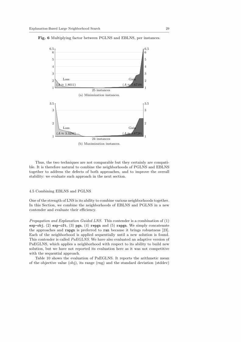
Explanation-Based Large Neighborhood Search 29
Fig. 6 Multiplying factor between PGLNS and EBLNS, per instances.
1 1
6.5 6.5
2 2
3 3
4 4
5 5
6 6
25 instances
(A ≈ 1.8011)
Loss
(A ≈ 7.6719)
Gain
(a) Minimization instances.
1 1
3.5 3.5
2 2
3 3
24 instances
(A ≈ 3.3296)
Loss
(A ≈ 3.6728)
Gain
(b) Maximization instances.
Thus, the two techniques are not comparable but they certainly are compati-ble. It is therefore natural to combine the neighborhoods of PGLNS and EBLNStogether to address the defects of both approaches, and to improve the overallstability: we evaluate such approach in the next section.
4.5 Combining EBLNS and PGLNS
One of the strength of LNS is its ability to combine various neighborhoods together.In this Section, we combine the neighborhoods of EBLNS and PGLNS in a newcontender and evaluate their efficiency.
Propagation and Explanation Guided LNS. This contender is a combination of (1)exp-obj, (2) exp-cft, (3) pgn, (4) repgn and (5) rapgn. We simply concatenatethe approaches and rapgn is preferred to ran because it brings robustness [23].Each of the neighborhood is applied sequentially until a new solution is found.This contender is called PaEGLNS. We have also evaluated an adaptive version ofPaEGLNS, which applies a neighborhood with respect to its ability to build newsolution, but we have not reported its evaluation here as it was not competitivewith the sequential approach.
Table 10 shows the evaluation of PaEGLNS. It reports the arithmetic meanof the objective value (obj), its range (rng) and the standard deviation (stddev)
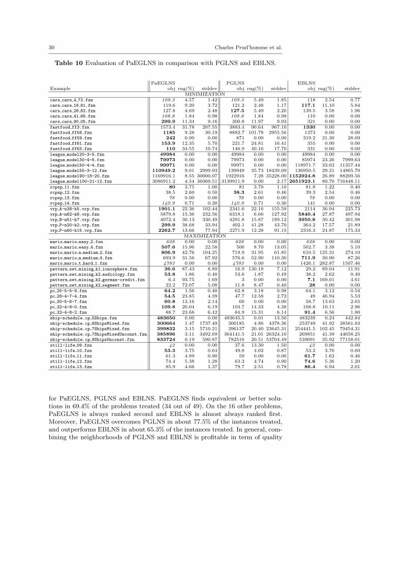
30 Charles Prud’homme et al.
Table 10 Evaluation of PaEGLNS in comparison with PGLNS and EBLNS.
PaEGLNS PGLNS EBLNSExample obj rng(%) stddev obj rng(%) stddev obj rng(%) stddev
MINIMIZATIONcars cars 4 72.fzn 109.3 4.57 1.42 109.3 5.49 1.85 118 2.54 0.77cars cars 16 81.fzn 119.6 9.20 3.72 121.2 2.48 1.17 117.1 11.10 5.84cars cars 26 82.fzn 127.8 4.69 2.48 127.5 5.49 2.20 139.5 3.58 1.96cars cars 41 66.fzn 108.8 1.84 0.98 108.8 1.84 0.98 110 0.00 0.00cars cars 90 05.fzn 299.9 11.34 9.16 300.8 11.97 9.93 321 0.00 0.00fastfood ff3.fzn 1573.4 31.78 207.55 3883.4 90.64 967.10 1330 0.00 0.00fastfood ff58.fzn 1185 9.28 30.19 8882.7 101.78 2955.56 1373 0.00 0.00fastfood ff59.fzn 242 0.00 0.00 871 0.00 0.00 319.2 21.30 28.09fastfood ff61.fzn 153.9 12.35 5.70 221.7 24.81 16.41 355 0.00 0.00fastfood ff63.fzn 110 34.55 10.74 146.9 40.16 17.70 331 0.00 0.00league model20-3-5.fzn 49984 0.00 0.00 49984 0.00 0.00 49984 0.00 0.00league model30-4-6.fzn 79973 0.00 0.00 79973 0.00 0.00 85974 23.26 7999.63league model50-4-4.fzn 99971 0.00 0.00 99971 0.00 0.00 118971.7 33.62 11357.44league model55-3-12.fzn 110949.2 9.01 2999.93 139949 35.73 18439.09 136950.5 29.21 14865.70league model90-18-20.fzn 1169916.1 8.55 30000.07 1922916 7.28 35228.00 1152924.8 26.89 88209.56league model100-21-12.fzn 3086911.2 4.54 36069.51 3139911.9 0.00 2.17 2651923.1 80.70 716448.11rcpsp 11.fzn 80 3.75 1.00 81 3.70 1.10 81.8 1.22 0.40rcpsp 12.fzn 38.5 2.60 0.50 38.3 2.61 0.46 39.3 2.54 0.46rcpsp 13.fzn 78 0.00 0.00 78 0.00 0.00 78 0.00 0.00rcpsp 14.fzn 140.9 0.71 0.30 140.9 0.71 0.30 141 0.00 0.00vrp A-n38-k5.vrp.fzn 1901.1 22.36 102.44 2341.6 22.16 155.59 2114 36.94 225.73vrp A-n62-k8.vrp.fzn 5879.8 15.36 232.56 6318.1 6.66 127.92 5840.4 27.87 497.94vrp B-n51-k7.vrp.fzn 4072.4 30.13 330.49 4291.8 15.87 189.12 3950.8 30.42 301.98vrp P-n20-k2.vrp.fzn 299.9 38.68 33.94 402.1 41.28 43.70 364.2 17.57 21.89vrp P-n60-k15.vrp.fzn 2262.7 13.66 77.94 2271.9 12.28 91.15 2316.3 24.87 175.33
MAXIMIZATIONmario mario easy 2.fzn 628 0.00 0.00 628 0.00 0.00 628 0.00 0.00mario mario easy 4.fzn 507.6 15.96 22.58 506 8.70 13.05 502.7 3.38 5.10mario mario n medium 2.fzn 806.9 42.76 104.25 719.9 31.95 61.85 610.5 125.31 274.10mario mario n medium 4.fzn 693.9 31.56 67.92 576.6 52.90 110.30 711.9 30.90 87.26mario mario t hard 1.fzn 4783 0.00 0.00 4783 0.00 0.00 1426.1 282.87 1507.46pattern set mining k1 ionosphere.fzn 36.6 87.43 8.89 16.9 130.18 7.12 29.2 89.04 11.91pattern set mining k2 audiology.fzn 53.8 1.86 0.40 53.6 1.87 0.49 38.2 2.62 0.40pattern set mining k2 german-credit.fzn 6.4 93.75 1.69 3 0.00 0.00 7.1 169.01 4.61pattern set mining k2 segment.fzn 22.2 72.07 5.08 11.8 8.47 0.40 28 0.00 0.00pc 25-5-5-9.fzn 64.2 1.56 0.40 62.8 3.18 0.98 64.1 3.12 0.54pc 28-4-7-4.fzn 54.5 23.85 4.39 47.7 12.58 2.72 49 46.94 5.53pc 30-5-6-7.fzn 60.8 13.16 2.14 60 0.00 0.00 58.7 13.63 2.65pc 32-4-8-0.fzn 109.8 20.04 6.19 104.7 14.33 4.38 108.8 10.11 2.96pc 32-4-8-2.fzn 88.7 23.68 6.42 84.9 15.31 6.14 91.4 6.56 1.80ship-schedule.cp 5Ships.fzn 483650 0.00 0.00 483645.5 0.01 13.50 483239 0.24 442.84ship-schedule.cp 6ShipsMixed.fzn 300664 1.47 1737.49 300185 4.86 4378.36 253749 41.92 38561.83ship-schedule.cp 7ShipsMixed.fzn 399832 3.15 5710.21 396137 20.40 23645.31 254441.5 102.45 79454.31ship-schedule.cp 7ShipsMixedUnconst.fzn 385896 3.11 3492.69 364141.5 21.01 26324.16 269851 41.39 44658.25ship-schedule.cp 8ShipsUnconst.fzn 833724 0.19 590.87 782516 20.51 53704.49 539091 35.92 77158.01still-life 09.fzn 42 0.00 0.00 37.6 13.30 1.50 42 0.00 0.00still-life 10.fzn 53.3 3.75 0.64 49.8 4.02 0.87 53.2 3.76 0.60still-life 11.fzn 61.3 4.89 0.90 59 0.00 0.00 61.7 1.62 0.46still-life 12.fzn 74.4 5.38 1.28 63.3 4.74 0.90 74.6 5.36 1.20still-life 13.fzn 85.9 4.66 1.37 79.7 2.51 0.78 86.4 6.94 2.01
for PaEGLNS, PGLNS and EBLNS. PaEGLNS finds equivalent or better solu-tions in 69.4% of the problems treated (34 out of 49). On the 16 other problems,PaEGLNS is always ranked second and EBLNS is almost always ranked first.Moreover, PaEGLNS overcomes PGLNS in about 77.5% of the instances treated,and outperforms EBLNS in about 65.3% of the instances treated. In general, com-bining the neighborhoods of PGLNS and EBLNS is profitable in term of quality

Explanation-Based Large Neighborhood Search 31
of the solutions but also in stability. In 58,8% of the instances better solved withPaEGLNS the range is less than 5%, which means that almost all runs find thesame last solution.
We now measure the gains and losses of using PaEGLNS instead of PGLNS orEBLNS. Figure 7 reports multiplying factor between PGLNS and PaEGLNS. Thefindings are unquestionable: PaEGLNS is clearly the most interesting approachwith respect to PGLNS. There is almost no degradation, only those linked torcpsp 12 and car cars 26 82, reflected in the plot by the non-zero light gray area(Figure 7(a)). The comparison with EBLNS (Figure 8) is mildly less advanta-
Fig. 7 Multiplying factor between PGLNS and PaEGLNS, per instance.
1 1
8 8
2 2
3 3
4 4
5 5
6 6
7 7
8 8
25 instances
(A ≈ 0.0049)
Loss
(A ≈ 9.7473)
Gain
(a) Minimization problems.
1 1
2.5 2.5
2 2
24 instances
(A ≈ 0)
Loss
(A ≈ 3.8159)
Gain
(b) Maximization problems.
geous, even though always widely in favor of PaEGLNS. There is no question thatPaEGLNS is the best choice.
These two generic approaches are complementary: on the one hand, PGLNSbuilds the graph of dependencies between variables and detects closely linked sub-parts of the problem treated. On the other hand, EBLNS helps to focus on easy-to-repair and easy-to-improve neighborhoods by revealing the relationships existingbetween the objective variable and the decision variables. Combining PGLNS andEBLNS benefits from the advantages of the two approaches: exploiting the struc-ture of the problems solved thank to both propagation and explanations, and bringmore stability in the solutions found.

32 Charles Prud’homme et al.
Fig. 8 Multiplying factor between EBLNS and PaEGLNS, per instance.
1 1
3 3
2 2
3 3
25 instances
(A ≈ 0.3291)
Loss
(A ≈ 3.9349)
Gain
(a) Minimization problems.
1 1
3.5 3.5
2 2
3 3
24 instances
(A ≈ 0.3114)
Loss
(A ≈ 4.0646)
Gain
(b) Maximization problems.
4.6 A deeper analysis
In the Section, we highlight some results that corroborate the previous ones foundso far. A figure is made of a plot and an histogram. The plot depicts the evolutionof the objective value along with the resolution time (in log scale) for the tenruns of the same approach (PGLNS, objLNS, cftLNS, EBLNS and PaEGLNS).The histogram reports the average repartition of the neighborhoods used to solvea given instance. The color coding is the following: exp-obj is in cross-patternedstyle, exp-cft is in slash-patterned style, ran is in plain white, pgn is in light gray,repgn is in dark gray and rapgn is in black.
On the Vehicle Routing Problem (Figure 9), the histograms indicate that agreat part of the intermediary solutions are found with the help of a pure randomneighborhood. Its proportion varies from 54% up to 83%. Regarding PaEGLNS,which finds the better solution, we observe the same phenomenon: even if its con-tribution is reduced, the random neighborhood helps finding almost half of thenew solutions. A comment is that random neighborhoods bring strong diversifica-tion and help solving the Vehicle Routing Problem but other neighborhoods playalso a role, such as exp-obj and pgn.
On the Restaurant Assignment Problem (Figure 10), where EBLNS worksfine, the portion of ran (< 1%) is negligible in comparison with exp-obj (34.2%)and exp-cft (65.7%). The stability of EBLNS on this instance is visible on theplot (Figure 10(d)). We roughly observe a similar phenomenon about cftLNS.objLNS, on the other hand, relies much more on randomness (54.7%). PaEGLNSnot only betters the objective in comparison with PGLNS and EBLNS but also
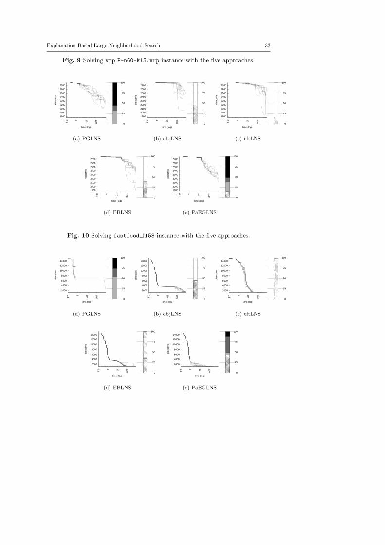
Explanation-Based Large Neighborhood Search 33
Fig. 9 Solving vrp P-n60-k15.vrp instance with the five approaches.
1900
2000
2100
2200
2300
2400
2500
2600
2700
0.1
1 10
100
obje
ctiv
e
time (log) 0
25
50
75
100
(a) PGLNS
1900
2000
2100
2200
2300
2400
2500
2600
2700
0.1
1 10
100
obje
ctiv
e
time (log) 0
25
50
75
100
(b) objLNS
1900
2000
2100
2200
2300
2400
2500
2600
2700
0.1
1 10
100
obje
ctiv
e
time (log) 0
25
50
75
100
(c) cftLNS
1900
2000
2100
2200
2300
2400
2500
2600
2700
0.1
1 10
100
obje
ctiv
e
time (log) 0
25
50
75
100
(d) EBLNS
1900
2000
2100
2200
2300
2400
2500
2600
2700
0.1
1 10
100
obje
ctiv
e
time (log) 0
25
50
75
100
(e) PaEGLNS
Fig. 10 Solving fastfood ff58 instance with the five approaches.
2000
4000
6000
8000
10000
12000
14000
0.1
1 10
100
obje
ctiv
e
time (log) 0
25
50
75
100
(a) PGLNS
2000
4000
6000
8000
10000
12000
14000
0.1
1 10
100
obje
ctiv
e
time (log) 0
25
50
75
100
(b) objLNS
2000
4000
6000
8000
10000
12000
14000
0.1
1 10
100
obje
ctiv
e
time (log) 0
25
50
75
100
(c) cftLNS
2000
4000
6000
8000
10000
12000
14000
0.1
1 10
100
obje
ctiv
e
time (log) 0
25
50
75
100
(d) EBLNS
2000
4000
6000
8000
10000
12000
14000
0.1
1 10
100
obje
ctiv
e
time (log) 0
25
50
75
100
(e) PaEGLNS
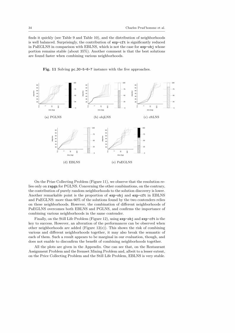
34 Charles Prud’homme et al.
finds it quickly (see Table 9 and Table 10), and the distribution of neighborhoodsis well balanced. Surprisingly, the contribution of exp-cft is significantly reducedin PaEGLNS in comparison with EBLNS, which is not the case for exp-obj whoseportion remains stable (about 35%). Another comment is that the best solutionsare found faster when combining various neighborhoods.
Fig. 11 Solving pc 30-5-6-7 instance with the five approaches.
30
35
40
45
50
55
60
0.1
1 10
100
obje
ctiv
e
time (log) 0
25
50
75
100
(a) PGLNS
30
35
40
45
50
55
60
0.1
1 10
100
obje
ctiv
e
time (log) 0
25
50
75
100
(b) objLNS
30
35
40
45
50
55
60
0.1
1 10
100
obje
ctiv
e
time (log) 0
25
50
75
100
(c) cftLNS
30
35
40
45
50
55
60
0.1
1 10
100
obje
ctiv
e
time (log) 0
25
50
75
100
(d) EBLNS
30
35
40
45
50
55
60
0.1
1 10
100
obje
ctiv
e
time (log) 0
25
50
75
100
(e) PaEGLNS
On the Prize Collecting Problem (Figure 11), we observe that the resolution re-lies only on rapgn for PGLNS. Concerning the other combinations, on the contrary,the contribution of purely random neighborhoods to the solution discovery is lower.Another remarkable point is the proportion of exp-obj and exp-cft in EBLNSand PaEGLNS: more than 60% of the solutions found by the two contenders relieson these neighborhoods. However, the combination of different neighborhoods ofPaEGLNS overcomes both EBLNS and PGLNS, and confirms the importance ofcombining various neighborhoods in the same contender.
Finally, on the Still Life Problem (Figure 12), using exp-obj and exp-cft is thekey to success. However, an alteration of the performances can be observed whenother neighborhoods are added (Figure 12(e)). This shows the risk of combiningvarious and different neighborhoods together, it may also break the semantic ofeach of them. Such a result appears to be marginal in our evaluation, though, anddoes not enable to disconfirm the benefit of combining neighborhoods together.
All the plots are given in the Appendix. One can see that, on the RestaurantAssignment Problem and the Itemset Mining Problem and, albeit to a lesser extent,on the Price Collecting Problem and the Still Life Problem, EBLNS is very stable.
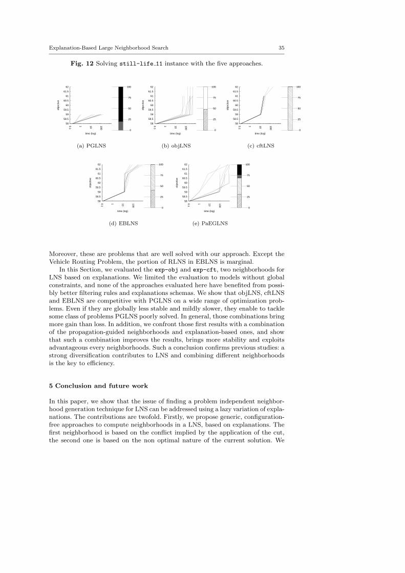
Explanation-Based Large Neighborhood Search 35
Fig. 12 Solving still-life 11 instance with the five approaches.
58
58.5
59
59.5
60
60.5
61
61.5
62
0.1
1 10
100
obje
ctiv
e
time (log) 0
25
50
75
100
(a) PGLNS
58
58.5
59
59.5
60
60.5
61
61.5
62
0.1
1 10
100
obje
ctiv
e
time (log) 0
25
50
75
100
(b) objLNS
58
58.5
59
59.5
60
60.5
61
61.5
62
0.1
1 10
100
obje
ctiv
e
time (log) 0
25
50
75
100
(c) cftLNS
58
58.5
59
59.5
60
60.5
61
61.5
62
0.1
1 10
100
obje
ctiv
e
time (log) 0
25
50
75
100
(d) EBLNS
58
58.5
59
59.5
60
60.5
61
61.5
62
0.1
1 10
100
obje
ctiv
e
time (log) 0
25
50
75
100
(e) PaEGLNS
Moreover, these are problems that are well solved with our approach. Except theVehicle Routing Problem, the portion of RLNS in EBLNS is marginal.
In this Section, we evaluated the exp-obj and exp-cft, two neighborhoods forLNS based on explanations. We limited the evaluation to models without globalconstraints, and none of the approaches evaluated here have benefited from possi-bly better filtering rules and explanations schemas. We show that objLNS, cftLNSand EBLNS are competitive with PGLNS on a wide range of optimization prob-lems. Even if they are globally less stable and mildly slower, they enable to tacklesome class of problems PGLNS poorly solved. In general, those combinations bringmore gain than loss. In addition, we confront those first results with a combinationof the propagation-guided neighborhoods and explanation-based ones, and showthat such a combination improves the results, brings more stability and exploitsadvantageous every neighborhoods. Such a conclusion confirms previous studies: astrong diversification contributes to LNS and combining different neighborhoodsis the key to efficiency.
5 Conclusion and future work
In this paper, we show that the issue of finding a problem independent neighbor-hood generation technique for LNS can be addressed using a lazy variation of expla-nations. The contributions are twofold. Firstly, we propose generic, configuration-free approaches to compute neighborhoods in a LNS, based on explanations. Thefirst neighborhood is based on the conflict implied by the application of the cut,the second one is based on the non optimal nature of the current solution. We

36 Charles Prud’homme et al.
address the diversification issues thanks to a set of heuristics for further selectingvariables mixing random approaches and explanation-based ones and show thatour approach is competitive with or even better than state-of-the-art algorithms,on a set of optimization problems. Secondly, we scheme explanation-based neigh-borhoods and propagation-guided ones, hoping that their behavior would be com-plementary. Finally, we assess the new contender on the same range of problems,and validate the combination to be very efficient and more stable.
Our results are encouraging and should be validated on a larger set of prob-lems. Moreover, we have to put things in perspective and analyze the influence ofthe model on the results, specifically on the Modified Car Sequencing Problem,where the results of PGLNS are quite surprising. Both the search strategy (howdecisions are selected) and the propagation engine (how events are relayed in theconstraint network) influence explanation-based neighborhoods and propagation-guided-ones. But, since the explanation of a domain reduction is not unique, ourapproach would benefit from more concise explanations, e.g., by enabling globalconstraints. Future works should focus on the diversification procedure, more par-ticularly plugging NoGoods in should be the key combination to speed up theexploration of nested search spaces. Finally, the lazy and asynchronous way tostore and compute explanations may be improved using incrementallity. It wouldalso be interesting to implement and evaluate such neighborhoods within a LCGsolver.
References
1. Kendall E. Atkins. An introduction to numerical analysis, 1989.2. Hadrien Cambazard and Narendra Jussien. Identifying and exploiting problem structures
using explanation-based constraint programming. Constraints, 11(4):295–313, 2006.3. Alain Chabrier, Emilie Danna, Claude Le Pape, and Laurent Perron. Solving a network
design problem. Annals of Operations Research, 130(1-4):217–239, 2004.4. Pedro J Copado-Mendez, Christian Blum, Gonzalo Guillen-Gosalbez, and Laureano
Jimenez. Application of large neighborhood search to strategic supply chain managementin the chemical industry. In Hybrid Metaheuristics, pages 335–352. Springer, 2013.
5. Emilie Danna and Laurent Perron. Structured vs. unstructured large neighborhood search:A case study on job-shop scheduling problems with earliness and tardiness costs. InFrancesca Rossi, editor, Principles and Practice of Constraint Programming CP 2003,volume 2833 of Lecture Notes in Computer Science, pages 817–821. Springer Berlin Hei-delberg, 2003.
6. Romuald Debruyne, Gerard Ferrand, Narendra Jussien, Willy Lesaint, Samir Ouis, andAlexandre Tessier. Correctness of constraint retraction algorithms. In FLAIRS’03: Six-teenth international Florida Artificial Intelligence Research Society conference, pages 172–176, St. Augustine, Florida, USA, May 2003. AAAI press.
7. Emrah Demir, Tolga Bektas, and Gilbert Laporte. An adaptive large neighborhood searchheuristic for the pollution-routing problem. European Journal of Operational Research,2012.
8. Ian P. Gent, Ian Miguel, and NeilC.A. Moore. Lazy explanations for constraint prop-agators. In Manuel Carro and Ricardo Pea, editors, Practical Aspects of DeclarativeLanguages, volume 5937 of Lecture Notes in Computer Science, pages 217–233. SpringerBerlin Heidelberg, 2010.
9. M. Ginsberg. Dynamic backtracking. Journal of Artificial Intelligence Research, 1:25–46,1993.
10. Daniel Godard, Philippe Laborie, and Wim Nuijten. Randomized large neighborhoodsearch for cumulative scheduling. In ICAPS, volume 5, pages 81–89, 2005.
11. Warwick Harvey and Joachim Schimpf. Bounds consistency techniques for long linearconstraints, 2002.

Explanation-Based Large Neighborhood Search 37
12. N. Jussien and O. Lhomme. Local search with constraint propagation and conflict-basedheuristics. Artificial Intelligence, 139(1):21–45, July 2002.
13. Narendra Jussien. The versatility of using explanations within constraint programming.Technical Report 03-04-INFO, 2003.
14. Narendra Jussien, Romuald Debruyne, and Patrice Boizumault. Maintaining arc-consistency within dynamic backtracking. In Principles and Practice of Constraint Pro-gramming (CP 2000), number 1894 in Lecture Notes in Computer Science, pages 249–261,Singapore, September 2000. Springer-Verlag.
15. Narendra Jussien and Olivier Lhomme. Dynamic domain splitting for numeric csps. InEuropean Conference on Artificial Intelligence (ECAI’98), pages 224–228, 1998.
16. Attila A Kovacs, Sophie N Parragh, Karl F Doerner, and Richard F Hartl. Adaptive largeneighborhood search for service technician routing and scheduling problems. Journal ofscheduling, 15(5):579–600, 2012.
17. P. Laborie and D. Godard. Self-adapting large neighborhood search:application to single-mode scheduling problems. In P. Baptiste, G. Kendall, A. Munier-Kordon, and F. Sourd,editors, In proceedings of the 3rd Multidisciplinary International Conference on Scheduling: Theory and Applications (MISTA 2007), 28 -31 August 2007, Paris, France, pages 276–284, 2007. Paper.
18. Jean-Baptiste Mairy, Yves Deville, and Pascal Van Hentenryck. Reinforced adaptive largeneighborhood search. In 8th Workshop on Local Search techniques in Constraint Satis-faction (LSCS2011), 2011.
19. Jean-Baptiste Mairy, Pierre Schaus, and Yves Deville. Generic adaptive heuristics forlarge neighborhood search. In 7th Workshop on Local Search Techniques in ConstraintSatisfaction (LSCS2010), 2010.
20. Yuri Malitsky, Deepak Mehta, Barry O’Sullivan, and Helmut Simonis. Tuning parame-ters of large neighborhood search for the machine reassignment problem. In Integrationof AI and OR Techniques in Constraint Programming for Combinatorial OptimizationProblems, pages 176–192. Springer, 2013.
21. Olga Ohrimenko, Peter J. Stuckey, and Michael Codish. Propagation via lazy clausegeneration. Constraints, 14(3):357–391, 2009.
22. Laurent Perron. Fast restart policies and large neighborhood search. In Francesca Rossi,editor, Principles and Practice of Constraint Programming at CP 2003, volume 2833 ofLecture Notes in Computer Science. Springer Berlin Heidelberg, 2003.
23. Laurent Perron and Paul Shaw. Combining forces to solve the car sequencing problem.In Jean-Charles Regin and Michel Rueher, editors, Integration of AI and OR Techniquesin Constraint Programming for Combinatorial Optimization Problems, volume 3011 ofLecture Notes in Computer Science, pages 225–239. Springer Berlin Heidelberg, 2004.
24. Laurent Perron, Paul Shaw, and Vincent Furnon. Propagation guided large neighborhoodsearch. In CP’04, pages 468–481, 2004.
25. David Pisinger and Stefan Ropke. Large neighborhood search. In Handbook of meta-heuristics, pages 399–419. Springer, 2010.
26. Cedric Pralet and Gerard Verfaillie. Travelling in the world of local searches in the space ofpartial assignments. In Jean-Charles Regin and Michel Rueher, editors, CPAIOR, volume3011 of Lecture Notes in Computer Science, pages 240–255. Springer, 2004.
27. P. Prosser. MAC-CBJ: maintaining arc consistency with conflict-directed backjumping.Technical Report Research Report/95/177, Dept. of Computer Science, University ofStrathclyde, 1995.
28. Charles Prud’homme and Jean-Guillaume Fages. Introduction to choco3. In 1st Work-shop on CPSolvers: Modeling, Applications, Integration, and Standardization, CP 2013,http://choco.emn.fr, 2013.
29. Andrea Roli, Stefano Benedettini, Thomas Stutzle, and Christian Blum. Large neighbour-hood search algorithms for the founder sequence reconstruction problem. Computers &operations research, 39(2):213–224, 2012.
30. T. Schiex and G. Verfaillie. Nogood recording for static and dynamic constraint satisfactionproblem. IJAIT, 3(2):187–207, 1994.
31. Paul Shaw. Using constraint programming and local search methods to solve vehiclerouting problems. In Michael Maher and Jean-Francois Puget, editors, Principles andPractice of Constraint Programming, CP98, volume 1520 of Lecture Notes in ComputerScience, pages 417–431. Springer Berlin Heidelberg, 1998.
32. Peter J. Stuckey. Lazy clause generation: Combining the power of sat and cp (and mip?)solving. In CPAIOR, pages 5–9, 2010.
38 Charles Prud’homme et al.
33. Gerard Verfaillie and Narendra Jussien. Constraint solving in uncertain and dynamicenvironments – a survey. Constraints, 10(3):253–281, 2005.
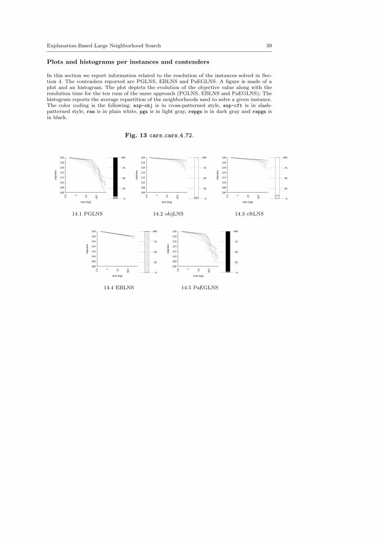
Explanation-Based Large Neighborhood Search 39
Plots and histograms per instances and contenders
In this section we report information related to the resolution of the instances solved in Sec-tion 4. The contenders reported are PGLNS, EBLNS and PaEGLNS. A figure is made of aplot and an histogram. The plot depicts the evolution of the objective value along with theresolution time for the ten runs of the same approach (PGLNS, EBLNS and PaEGLNS); Thehistogram reports the average repartition of the neighborhoods used to solve a given instance.The color coding is the following: exp-obj is in cross-patterned style, exp-cft is in slash-patterned style, ran is in plain white, pgn is in light gray, repgn is in dark gray and rapgn isin black.
Fig. 13 cars cars 4 72.
106
108
110
112
114
116
118
120
0.1
1 10
100
obje
ctiv
e
time (log) 0
25
50
75
100
14.1 PGLNS
106
108
110
112
114
116
118
120
0.1
1 10
100
obje
ctiv
e
time (log) 0
25
50
75
100
14.2 objLNS
106
108
110
112
114
116
118
120 0.1
1 10
100
obje
ctiv
e
time (log) 0
25
50
75
100
14.3 cftLNS
106
108
110
112
114
116
118
120
0.1
1 10
100
obje
ctiv
e
time (log) 0
25
50
75
100
14.4 EBLNS
106
108
110
112
114
116
118
120
0.1
1 10
100
obje
ctiv
e
time (log) 0
25
50
75
100
14.5 PaEGLNS
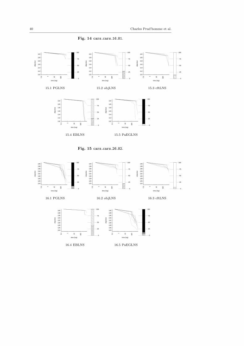
40 Charles Prud’homme et al.
Fig. 14 cars cars 16 81.
110
112
114
116
118
120
122
0.1
1 10
100
obje
ctiv
e
time (log) 0
25
50
75
100
15.1 PGLNS
110
112
114
116
118
120
122
0.1
1 10
100
obje
ctiv
e
time (log) 0
25
50
75
100
15.2 objLNS
110
112
114
116
118
120
122
0.1
1 10
100
obje
ctiv
e
time (log) 0
25
50
75
100
15.3 cftLNS
110
112
114
116
118
120
122
0.1
1 10
100
obje
ctiv
e
time (log) 0
25
50
75
100
15.4 EBLNS
110
112
114
116
118
120
122
0.1
1 10
100
obje
ctiv
e
time (log) 0
25
50
75
100
15.5 PaEGLNS
Fig. 15 cars cars 26 82.
124
126
128
130
132
134
136
138
140
0.1
1 10
100
obje
ctiv
e
time (log) 0
25
50
75
100
16.1 PGLNS
124
126
128
130
132
134
136
138
140
0.1
1 10
100
obje
ctiv
e
time (log) 0
25
50
75
100
16.2 objLNS
124
126
128
130
132
134
136
138
140
0.1
1 10
100
obje
ctiv
e
time (log) 0
25
50
75
100
16.3 cftLNS
124
126
128
130
132
134
136
138
140
0.1
1 10
100
obje
ctiv
e
time (log) 0
25
50
75
100
16.4 EBLNS
124
126
128
130
132
134
136
138
140
0.1
1 10
100
obje
ctiv
e
time (log) 0
25
50
75
100
16.5 PaEGLNS
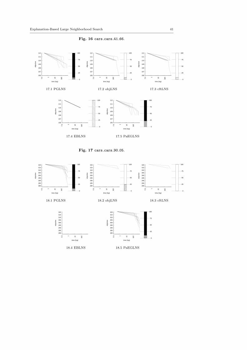
Explanation-Based Large Neighborhood Search 41
Fig. 16 cars cars 41 66.
106
107
108
109
110
111
112
0.1
1 10
100
obje
ctiv
e
time (log) 0
25
50
75
100
17.1 PGLNS
106
107
108
109
110
111
112
0.1
1 10
100
obje
ctiv
e
time (log) 0
25
50
75
100
17.2 objLNS
106
107
108
109
110
111
112
0.1
1 10
100
obje
ctiv
e
time (log) 0
25
50
75
100
17.3 cftLNS
106
107
108
109
110
111
112
0.1
1 10
100
obje
ctiv
e
time (log) 0
25
50
75
100
17.4 EBLNS
106
107
108
109
110
111
112
0.1
1 10
100
obje
ctiv
e
time (log) 0
25
50
75
100
17.5 PaEGLNS
Fig. 17 cars cars 90 05.
280
285
290
295
300
305
310
315
320
0.1
1 10
100
obje
ctiv
e
time (log) 0
25
50
75
100
18.1 PGLNS
280
285
290
295
300
305
310
315
320
0.1
1 10
100
obje
ctiv
e
time (log) 0
25
50
75
100
18.2 objLNS
280
285
290
295
300
305
310
315
320
0.1
1 10
100
obje
ctiv
e
time (log) 0
25
50
75
100
18.3 cftLNS
280
285
290
295
300
305
310
315
320
0.1
1 10
100
obje
ctiv
e
time (log)
18.4 EBLNS
280
285
290
295
300
305
310
315
320
0.1
1 10
100
obje
ctiv
e
time (log) 0
25
50
75
100
18.5 PaEGLNS

42 Charles Prud’homme et al.
Fig. 18 fastfood ff3.
2000
3000
4000
5000
6000
7000
0.1
1 10
100
obje
ctiv
e
time (log) 0
25
50
75
100
19.1 PGLNS
2000
3000
4000
5000
6000
7000
0.1
1 10
100
obje
ctiv
e
time (log) 0
25
50
75
100
19.2 objLNS
2000
3000
4000
5000
6000
7000
0.1
1 10
100
obje
ctiv
e
time (log) 0
25
50
75
100
19.3 cftLNS
2000
3000
4000
5000
6000
7000
0.1
1 10
100
obje
ctiv
e
time (log) 0
25
50
75
100
19.4 EBLNS
2000
3000
4000
5000
6000
7000
0.1
1 10
100
obje
ctiv
e
time (log) 0
25
50
75
100
19.5 PaEGLNS
Fig. 19 fastfood ff58.
2000
4000
6000
8000
10000
12000
14000
0.1
1 10
100
obje
ctiv
e
time (log) 0
25
50
75
100
20.1 PGLNS
2000
4000
6000
8000
10000
12000
14000
0.1
1 10
100
obje
ctiv
e
time (log) 0
25
50
75
100
20.2 objLNS
2000
4000
6000
8000
10000
12000
14000
0.1
1 10
100
obje
ctiv
e
time (log) 0
25
50
75
100
20.3 cftLNS
2000
4000
6000
8000
10000
12000
14000
0.1
1 10
100
obje
ctiv
e
time (log) 0
25
50
75
100
20.4 EBLNS
2000
4000
6000
8000
10000
12000
14000
0.1
1 10
100
obje
ctiv
e
time (log) 0
25
50
75
100
20.5 PaEGLNS
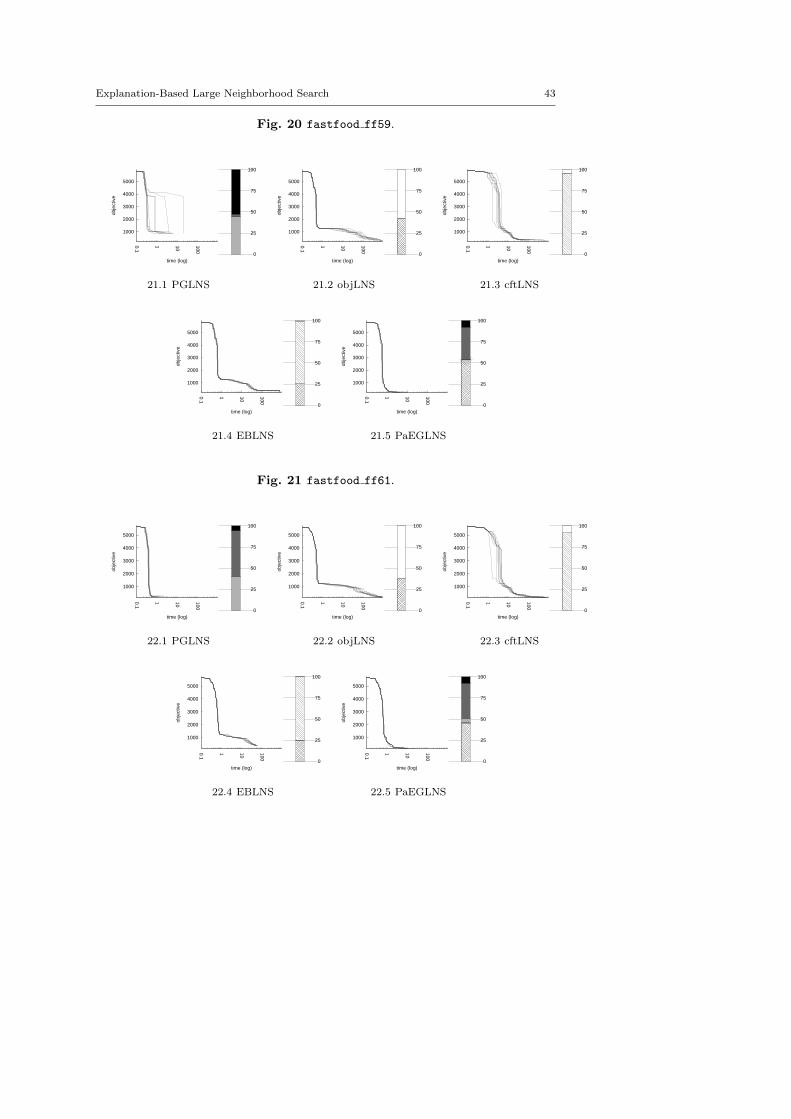
Explanation-Based Large Neighborhood Search 43
Fig. 20 fastfood ff59.
1000
2000
3000
4000
5000
0.1
1 10
100
obje
ctiv
e
time (log) 0
25
50
75
100
21.1 PGLNS
1000
2000
3000
4000
5000
0.1
1 10
100
obje
ctiv
e
time (log) 0
25
50
75
100
21.2 objLNS
1000
2000
3000
4000
5000
0.1
1 10
100
obje
ctiv
e
time (log) 0
25
50
75
100
21.3 cftLNS
1000
2000
3000
4000
5000
0.1
1 10
100
obje
ctiv
e
time (log) 0
25
50
75
100
21.4 EBLNS
1000
2000
3000
4000
5000
0.1
1 10
100
obje
ctiv
e
time (log) 0
25
50
75
100
21.5 PaEGLNS
Fig. 21 fastfood ff61.
1000
2000
3000
4000
5000
0.1
1 10
100
obje
ctiv
e
time (log) 0
25
50
75
100
22.1 PGLNS
1000
2000
3000
4000
5000
0.1
1 10
100
obje
ctiv
e
time (log) 0
25
50
75
100
22.2 objLNS
1000
2000
3000
4000
5000
0.1
1 10
100
obje
ctiv
e
time (log) 0
25
50
75
100
22.3 cftLNS
1000
2000
3000
4000
5000
0.1
1 10
100
obje
ctiv
e
time (log) 0
25
50
75
100
22.4 EBLNS
1000
2000
3000
4000
5000
0.1
1 10
100
obje
ctiv
e
time (log) 0
25
50
75
100
22.5 PaEGLNS
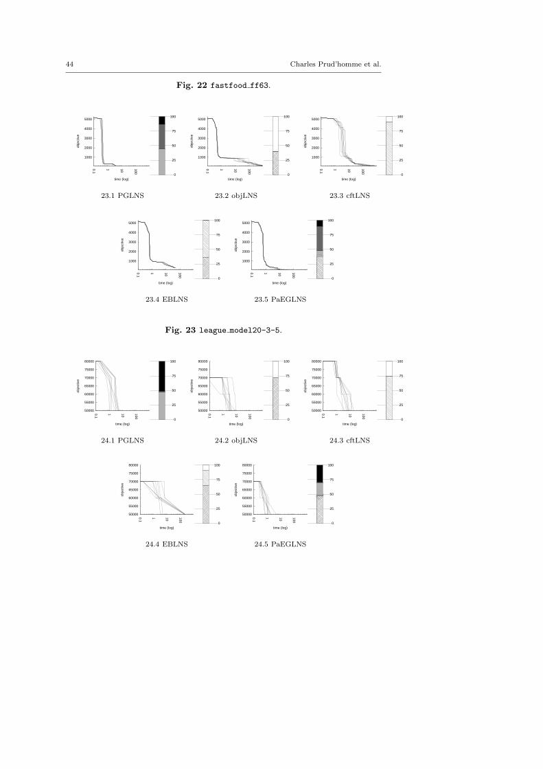
44 Charles Prud’homme et al.
Fig. 22 fastfood ff63.
1000
2000
3000
4000
5000
0.1
1 10
100
obje
ctiv
e
time (log) 0
25
50
75
100
23.1 PGLNS
1000
2000
3000
4000
5000
0.1
1 10
100
obje
ctiv
e
time (log) 0
25
50
75
100
23.2 objLNS
1000
2000
3000
4000
5000
0.1
1 10
100
obje
ctiv
e
time (log) 0
25
50
75
100
23.3 cftLNS
1000
2000
3000
4000
5000
0.1
1 10
100
obje
ctiv
e
time (log) 0
25
50
75
100
23.4 EBLNS
1000
2000
3000
4000
5000
0.1
1 10
100
obje
ctiv
e
time (log) 0
25
50
75
100
23.5 PaEGLNS
Fig. 23 league model20-3-5.
50000
55000
60000
65000
70000
75000
80000
0.1
1 10
100
obje
ctiv
e
time (log) 0
25
50
75
100
24.1 PGLNS
50000
55000
60000
65000
70000
75000
80000
0.1
1 10
100
obje
ctiv
e
time (log) 0
25
50
75
100
24.2 objLNS
50000
55000
60000
65000
70000
75000
80000
0.1
1 10
100
obje
ctiv
e
time (log) 0
25
50
75
100
24.3 cftLNS
50000
55000
60000
65000
70000
75000
80000
0.1
1 10
100
obje
ctiv
e
time (log) 0
25
50
75
100
24.4 EBLNS
50000
55000
60000
65000
70000
75000
80000
0.1
1 10
100
obje
ctiv
e
time (log) 0
25
50
75
100
24.5 PaEGLNS

Explanation-Based Large Neighborhood Search 45
Fig. 24 league model30-4-6.
80000
90000
100000
110000
120000
130000
140000
150000
0.1
1 10
100
obje
ctiv
e
time (log) 0
25
50
75
100
25.1 PGLNS
80000
90000
100000
110000
120000
130000
140000
150000
0.1
1 10
100
obje
ctiv
e
time (log) 0
25
50
75
100
25.2 objLNS
80000
90000
100000
110000
120000
130000
140000
150000
0.1
1 10
100
obje
ctiv
e
time (log) 0
25
50
75
100
25.3 cftLNS
80000
90000
100000
110000
120000
130000
140000
150000
0.1
1 10
100
obje
ctiv
e
time (log) 0
25
50
75
100
25.4 EBLNS
80000
90000
100000
110000
120000
130000
140000
150000
0.1
1 10
100
obje
ctiv
e
time (log) 0
25
50
75
100
25.5 PaEGLNS
Fig. 25 league model50-4-4.
100000
110000
120000
130000
140000
150000
160000
0.1
1 10
100
obje
ctiv
e
time (log) 0
25
50
75
100
26.1 PGLNS
100000
110000
120000
130000
140000
150000
160000
0.1
1 10
100
obje
ctiv
e
time (log) 0
25
50
75
100
26.2 objLNS
100000
110000
120000
130000
140000
150000
160000
0.1
1 10
100
obje
ctiv
e
time (log) 0
25
50
75
100
26.3 cftLNS
100000
110000
120000
130000
140000
150000
160000
0.1
1 10
100
obje
ctiv
e
time (log) 0
25
50
75
100
26.4 EBLNS
100000
110000
120000
130000
140000
150000
160000
0.1
1 10
100
obje
ctiv
e
time (log) 0
25
50
75
100
26.5 PaEGLNS

46 Charles Prud’homme et al.
Fig. 26 league model55-3-12.
110000
120000
130000
140000
150000
160000
0.1
1 10
100
obje
ctiv
e
time (log) 0
25
50
75
100
27.1 PGLNS
110000
120000
130000
140000
150000
160000
0.1
1 10
100
obje
ctiv
e
time (log) 0
25
50
75
100
27.2 objLNS
110000
120000
130000
140000
150000
160000
0.1
1 10
100
obje
ctiv
e
time (log) 0
25
50
75
100
27.3 cftLNS
110000
120000
130000
140000
150000
160000
0.1
1 10
100
obje
ctiv
e
time (log) 0
25
50
75
100
27.4 EBLNS
110000
120000
130000
140000
150000
160000
0.1
1 10
100
obje
ctiv
e
time (log) 0
25
50
75
100
27.5 PaEGLNS
Fig. 27 league model90-18-20.
800000
1e+06
1.2e+06
1.4e+06
1.6e+06
1.8e+06
2e+06
0.1
1 10
100
obje
ctiv
e
time (log) 0
25
50
75
100
28.1 PGLNS
800000
1e+06
1.2e+06
1.4e+06
1.6e+06
1.8e+06
2e+06
0.1
1 10
100
obje
ctiv
e
time (log) 0
25
50
75
100
28.2 objLNS
800000
1e+06
1.2e+06
1.4e+06
1.6e+06
1.8e+06
2e+06
0.1
1 10
100
obje
ctiv
e
time (log) 0
25
50
75
100
28.3 cftLNS
800000
1e+06
1.2e+06
1.4e+06
1.6e+06
1.8e+06
2e+06
0.1
1 10
100
obje
ctiv
e
time (log) 0
25
50
75
100
28.4 EBLNS
800000
1e+06
1.2e+06
1.4e+06
1.6e+06
1.8e+06
2e+06
0.1
1 10
100
obje
ctiv
e
time (log) 0
25
50
75
100
28.5 PaEGLNS
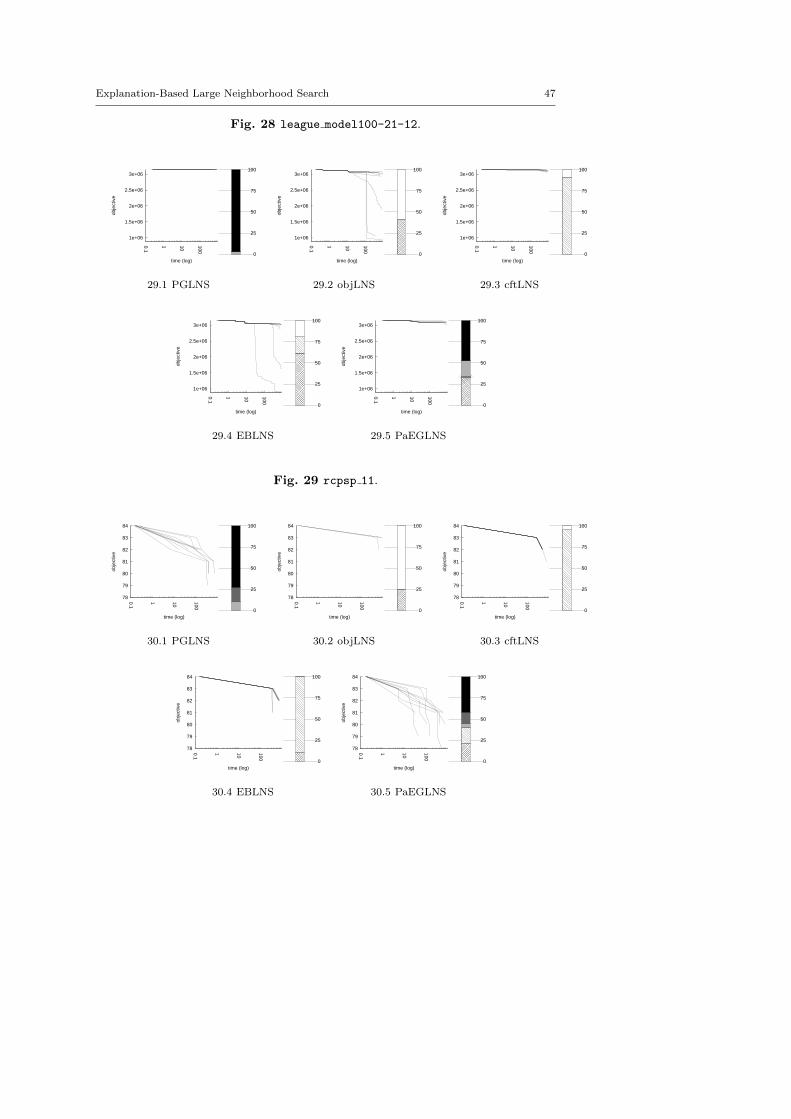
Explanation-Based Large Neighborhood Search 47
Fig. 28 league model100-21-12.
1e+06
1.5e+06
2e+06
2.5e+06
3e+06
0.1
1 10
100
obje
ctiv
e
time (log) 0
25
50
75
100
29.1 PGLNS
1e+06
1.5e+06
2e+06
2.5e+06
3e+06
0.1
1 10
100
obje
ctiv
e
time (log) 0
25
50
75
100
29.2 objLNS
1e+06
1.5e+06
2e+06
2.5e+06
3e+06
0.1
1 10
100
obje
ctiv
e
time (log) 0
25
50
75
100
29.3 cftLNS
1e+06
1.5e+06
2e+06
2.5e+06
3e+06
0.1
1 10
100
obje
ctiv
e
time (log) 0
25
50
75
100
29.4 EBLNS
1e+06
1.5e+06
2e+06
2.5e+06
3e+06
0.1
1 10
100
obje
ctiv
e
time (log) 0
25
50
75
100
29.5 PaEGLNS
Fig. 29 rcpsp 11.
78
79
80
81
82
83
84
0.1
1 10
100
obje
ctiv
e
time (log) 0
25
50
75
100
30.1 PGLNS
78
79
80
81
82
83
84
0.1
1 10
100
obje
ctiv
e
time (log) 0
25
50
75
100
30.2 objLNS
78
79
80
81
82
83
84
0.1
1 10
100
obje
ctiv
e
time (log) 0
25
50
75
100
30.3 cftLNS
78
79
80
81
82
83
84
0.1
1 10
100
obje
ctiv
e
time (log) 0
25
50
75
100
30.4 EBLNS
78
79
80
81
82
83
84
0.1
1 10
100
obje
ctiv
e
time (log) 0
25
50
75
100
30.5 PaEGLNS
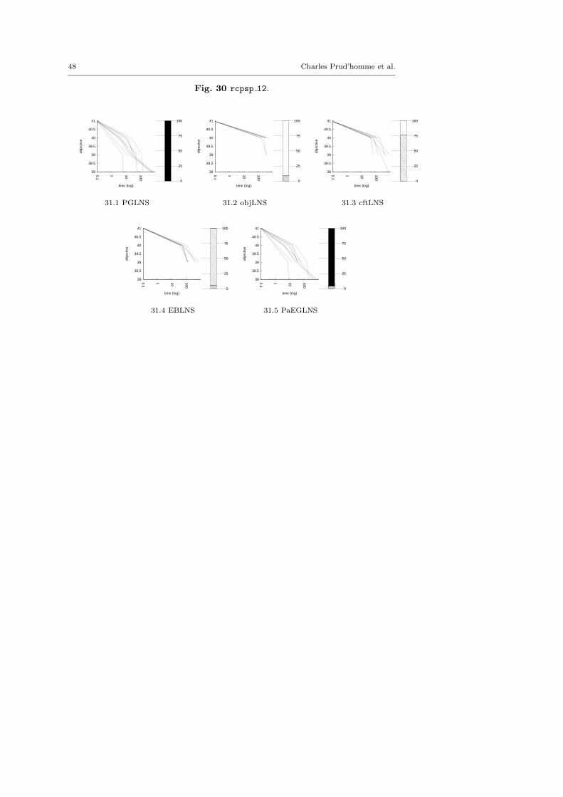
48 Charles Prud’homme et al.
Fig. 30 rcpsp 12.
38
38.5
39
39.5
40
40.5
41
0.1
1 10
100
obje
ctiv
e
time (log) 0
25
50
75
100
31.1 PGLNS
38
38.5
39
39.5
40
40.5
41
0.1
1 10
100
obje
ctiv
e
time (log) 0
25
50
75
100
31.2 objLNS
38
38.5
39
39.5
40
40.5
41
0.1
1 10
100
obje
ctiv
e
time (log) 0
25
50
75
100
31.3 cftLNS
38
38.5
39
39.5
40
40.5
41
0.1
1 10
100
obje
ctiv
e
time (log) 0
25
50
75
100
31.4 EBLNS
38
38.5
39
39.5
40
40.5
41
0.1
1 10
100
obje
ctiv
e
time (log) 0
25
50
75
100
31.5 PaEGLNS
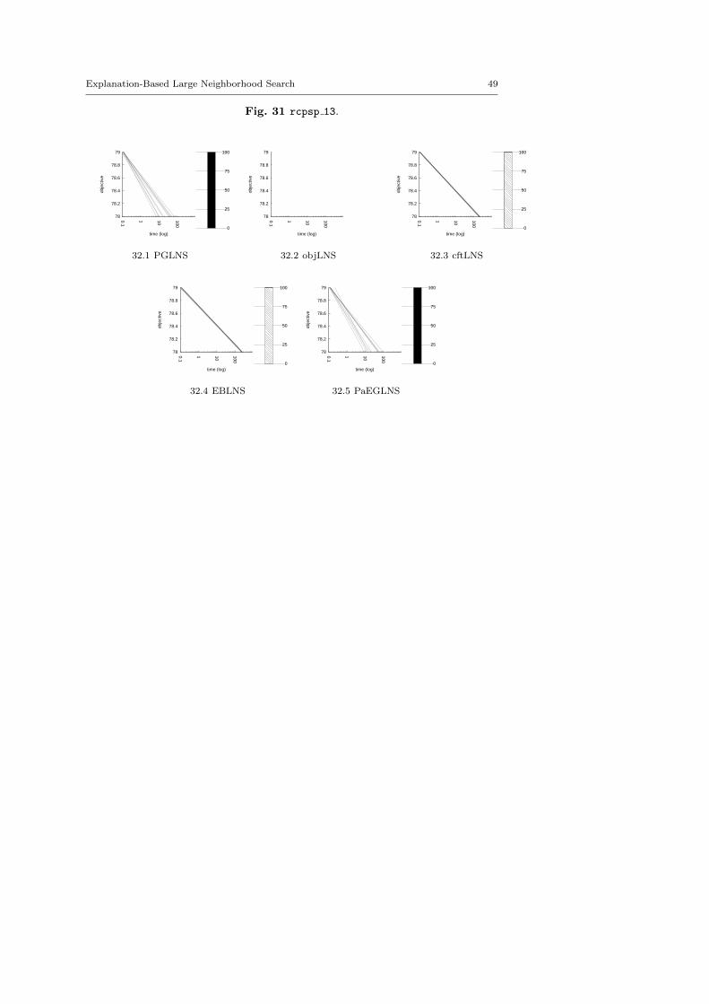
Explanation-Based Large Neighborhood Search 49
Fig. 31 rcpsp 13.
78
78.2
78.4
78.6
78.8
79
0.1
1 10
100
obje
ctiv
e
time (log) 0
25
50
75
100
32.1 PGLNS
78
78.2
78.4
78.6
78.8
79
0.1
1 10
100
obje
ctiv
e
time (log)
32.2 objLNS
78
78.2
78.4
78.6
78.8
79
0.1
1 10
100
obje
ctiv
e
time (log) 0
25
50
75
100
32.3 cftLNS
78
78.2
78.4
78.6
78.8
79
0.1
1 10
100
obje
ctiv
e
time (log) 0
25
50
75
100
32.4 EBLNS
78
78.2
78.4
78.6
78.8
79
0.1
1 10
100
obje
ctiv
e
time (log) 0
25
50
75
100
32.5 PaEGLNS
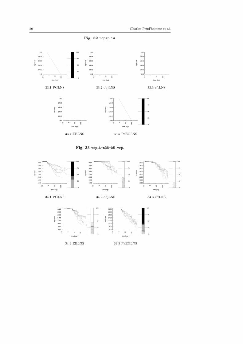
50 Charles Prud’homme et al.
Fig. 32 rcpsp 14.
140
140.2
140.4
140.6
140.8
141
0.1
1 10
100
obje
ctiv
e
time (log) 0
25
50
75
100
33.1 PGLNS
140
140.2
140.4
140.6
140.8
141
0.1
1 10
100
obje
ctiv
e
time (log)
33.2 objLNS
140
140.2
140.4
140.6
140.8
141
0.1
1 10
100
obje
ctiv
e
time (log)
33.3 cftLNS
140
140.2
140.4
140.6
140.8
141
0.1
1 10
100
obje
ctiv
e
time (log)
33.4 EBLNS
140
140.2
140.4
140.6
140.8
141
0.1
1 10
100
obje
ctiv
e
time (log) 0
25
50
75
100
33.5 PaEGLNS
Fig. 33 vrp A-n38-k5.vrp.
1600
1800
2000
2200
2400
2600
2800
3000
0.1
1 10
100
obje
ctiv
e
time (log) 0
25
50
75
100
34.1 PGLNS
1600
1800
2000
2200
2400
2600
2800
3000
0.1
1 10
100
obje
ctiv
e
time (log) 0
25
50
75
100
34.2 objLNS
1600
1800
2000
2200
2400
2600
2800
3000
0.1
1 10
100
obje
ctiv
e
time (log) 0
25
50
75
100
34.3 cftLNS
1600
1800
2000
2200
2400
2600
2800
3000
0.1
1 10
100
obje
ctiv
e
time (log) 0
25
50
75
100
34.4 EBLNS
1600
1800
2000
2200
2400
2600
2800
3000
0.1
1 10
100
obje
ctiv
e
time (log) 0
25
50
75
100
34.5 PaEGLNS

Explanation-Based Large Neighborhood Search 51
Fig. 34 vrp A-n62-k8.vrp.
5000
5500
6000
6500
7000
0.1
1 10
100
obje
ctiv
e
time (log) 0
25
50
75
100
35.1 PGLNS
5000
5500
6000
6500
7000
0.1
1 10
100
obje
ctiv
e
time (log) 0
25
50
75
100
35.2 objLNS
5000
5500
6000
6500
7000
0.1
1 10
100
obje
ctiv
e
time (log) 0
25
50
75
100
35.3 cftLNS
5000
5500
6000
6500
7000
0.1
1 10
100
obje
ctiv
e
time (log) 0
25
50
75
100
35.4 EBLNS
5000
5500
6000
6500
7000
0.1
1 10
100
obje
ctiv
e
time (log) 0
25
50
75
100
35.5 PaEGLNS
Fig. 35 vrp B-n51-k7.vrp.
3500
4000
4500
5000
0.1
1 10
100
obje
ctiv
e
time (log) 0
25
50
75
100
36.1 PGLNS
3500
4000
4500
5000
0.1
1 10
100
obje
ctiv
e
time (log) 0
25
50
75
100
36.2 objLNS
3500
4000
4500
5000
0.1
1 10
100
obje
ctiv
e
time (log) 0
25
50
75
100
36.3 cftLNS
3500
4000
4500
5000
0.1
1 10
100
obje
ctiv
e
time (log) 0
25
50
75
100
36.4 EBLNS
3500
4000
4500
5000
0.1
1 10
100
obje
ctiv
e
time (log) 0
25
50
75
100
36.5 PaEGLNS

52 Charles Prud’homme et al.
Fig. 36 vrp P-n20-k2.vrp.
300
400
500
600
700
800
900
1000
0.1
1 10
100
obje
ctiv
e
time (log) 0
25
50
75
100
37.1 PGLNS
300
400
500
600
700
800
900
1000
0.1
1 10
100
obje
ctiv
e
time (log) 0
25
50
75
100
37.2 objLNS
300
400
500
600
700
800
900
1000
0.1
1 10
100
obje
ctiv
e
time (log) 0
25
50
75
100
37.3 cftLNS
300
400
500
600
700
800
900
1000
0.1
1 10
100
obje
ctiv
e
time (log) 0
25
50
75
100
37.4 EBLNS
300
400
500
600
700
800
900
1000
0.1
1 10
100
obje
ctiv
e
time (log) 0
25
50
75
100
37.5 PaEGLNS
Fig. 37 vrp P-n60-k15.vrp.
1900
2000
2100
2200
2300
2400
2500
2600
2700
0.1
1 10
100
obje
ctiv
e
time (log) 0
25
50
75
100
38.1 PGLNS
1900
2000
2100
2200
2300
2400
2500
2600
2700
0.1
1 10
100
obje
ctiv
e
time (log) 0
25
50
75
100
38.2 objLNS
1900
2000
2100
2200
2300
2400
2500
2600
2700
0.1
1 10
100
obje
ctiv
e
time (log) 0
25
50
75
100
38.3 cftLNS
1900
2000
2100
2200
2300
2400
2500
2600
2700
0.1
1 10
100
obje
ctiv
e
time (log) 0
25
50
75
100
38.4 EBLNS
1900
2000
2100
2200
2300
2400
2500
2600
2700
0.1
1 10
100
obje
ctiv
e
time (log) 0
25
50
75
100
38.5 PaEGLNS
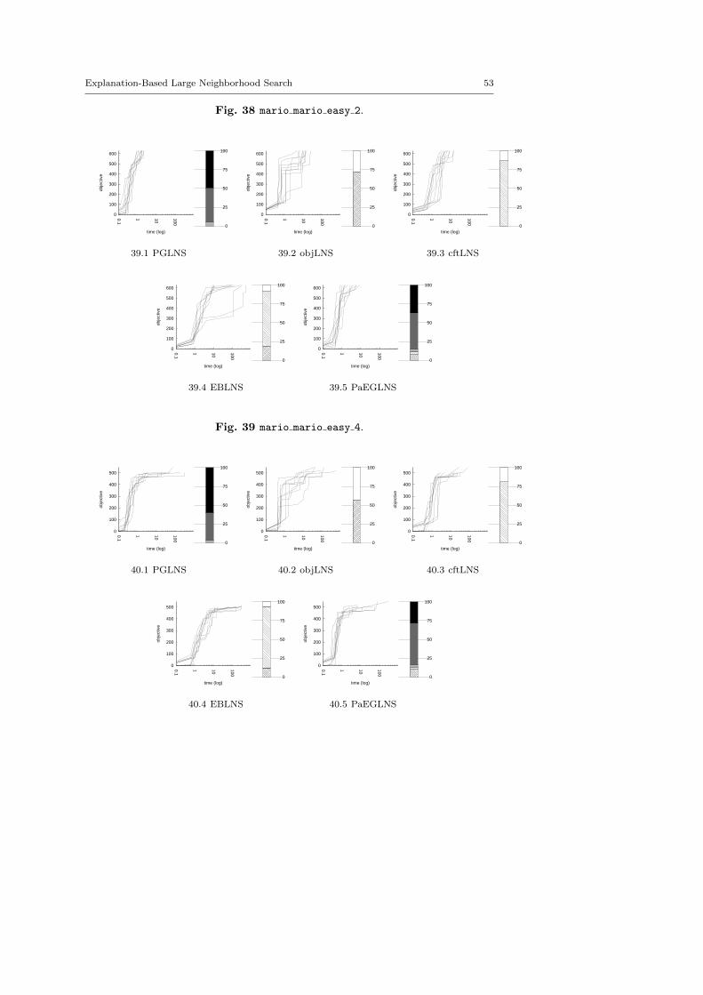
Explanation-Based Large Neighborhood Search 53
Fig. 38 mario mario easy 2.
0
100
200
300
400
500
600
0.1
1 10
100
obje
ctiv
e
time (log) 0
25
50
75
100
39.1 PGLNS
0
100
200
300
400
500
600
0.1
1 10
100
obje
ctiv
e
time (log) 0
25
50
75
100
39.2 objLNS
0
100
200
300
400
500
600
0.1
1 10
100
obje
ctiv
e
time (log) 0
25
50
75
100
39.3 cftLNS
0
100
200
300
400
500
600
0.1
1 10
100
obje
ctiv
e
time (log) 0
25
50
75
100
39.4 EBLNS
0
100
200
300
400
500
600
0.1
1 10
100
obje
ctiv
e
time (log) 0
25
50
75
100
39.5 PaEGLNS
Fig. 39 mario mario easy 4.
0
100
200
300
400
500
0.1
1 10
100
obje
ctiv
e
time (log) 0
25
50
75
100
40.1 PGLNS
0
100
200
300
400
500
0.1
1 10
100
obje
ctiv
e
time (log) 0
25
50
75
100
40.2 objLNS
0
100
200
300
400
500
0.1
1 10
100
obje
ctiv
e
time (log) 0
25
50
75
100
40.3 cftLNS
0
100
200
300
400
500
0.1
1 10
100
obje
ctiv
e
time (log) 0
25
50
75
100
40.4 EBLNS
0
100
200
300
400
500
0.1
1 10
100
obje
ctiv
e
time (log) 0
25
50
75
100
40.5 PaEGLNS
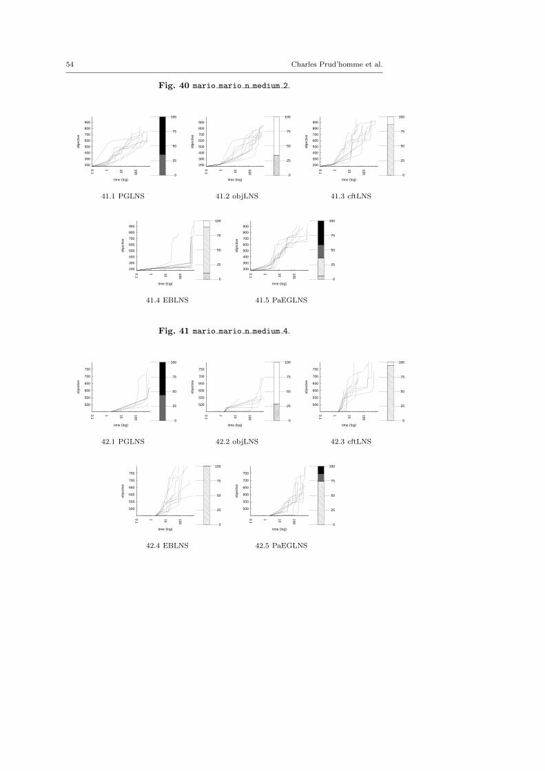
54 Charles Prud’homme et al.
Fig. 40 mario mario n medium 2.
200
300
400
500
600
700
800
900
0.1
1 10
100
obje
ctiv
e
time (log) 0
25
50
75
100
41.1 PGLNS
200
300
400
500
600
700
800
900
0.1
1 10
100
obje
ctiv
e
time (log) 0
25
50
75
100
41.2 objLNS
200
300
400
500
600
700
800
900
0.1
1 10
100
obje
ctiv
e
time (log) 0
25
50
75
100
41.3 cftLNS
200
300
400
500
600
700
800
900
0.1
1 10
100
obje
ctiv
e
time (log) 0
25
50
75
100
41.4 EBLNS
200
300
400
500
600
700
800
900
0.1
1 10
100
obje
ctiv
e
time (log) 0
25
50
75
100
41.5 PaEGLNS
Fig. 41 mario mario n medium 4.
500
550
600
650
700
750
0.1
1 10
100
obje
ctiv
e
time (log) 0
25
50
75
100
42.1 PGLNS
500
550
600
650
700
750
0.1
1 10
100
obje
ctiv
e
time (log) 0
25
50
75
100
42.2 objLNS
500
550
600
650
700
750
0.1
1 10
100
obje
ctiv
e
time (log) 0
25
50
75
100
42.3 cftLNS
500
550
600
650
700
750
0.1
1 10
100
obje
ctiv
e
time (log) 0
25
50
75
100
42.4 EBLNS
500
550
600
650
700
750
0.1
1 10
100
obje
ctiv
e
time (log) 0
25
50
75
100
42.5 PaEGLNS
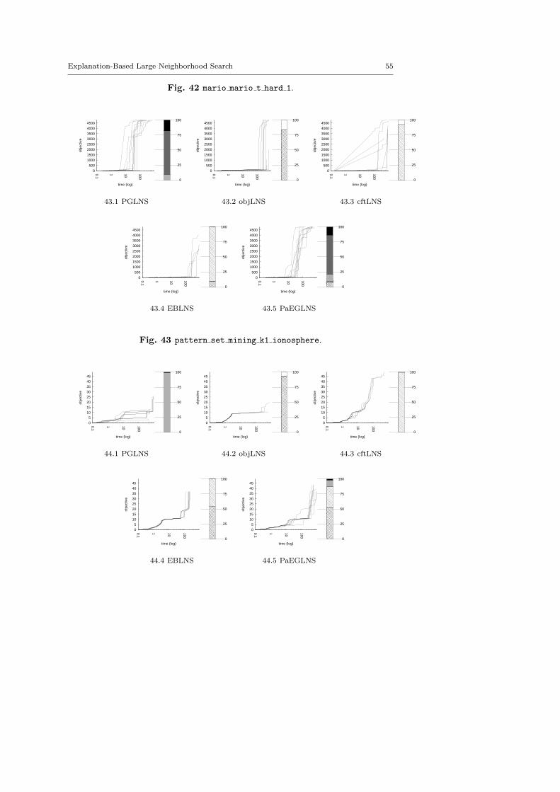
Explanation-Based Large Neighborhood Search 55
Fig. 42 mario mario t hard 1.
0
500
1000
1500
2000
2500
3000
3500
4000
4500
0.1
1 10
100
obje
ctiv
e
time (log) 0
25
50
75
100
43.1 PGLNS
0
500
1000
1500
2000
2500
3000
3500
4000
4500
0.1
1 10
100
obje
ctiv
e
time (log) 0
25
50
75
100
43.2 objLNS
0
500
1000
1500
2000
2500
3000
3500
4000
4500
0.1
1 10
100
obje
ctiv
e
time (log) 0
25
50
75
100
43.3 cftLNS
0
500
1000
1500
2000
2500
3000
3500
4000
4500
0.1
1 10
100
obje
ctiv
e
time (log) 0
25
50
75
100
43.4 EBLNS
0
500
1000
1500
2000
2500
3000
3500
4000
4500
0.1
1 10
100
obje
ctiv
e
time (log) 0
25
50
75
100
43.5 PaEGLNS
Fig. 43 pattern set mining k1 ionosphere.
0
5
10
15
20
25
30
35
40
45
0.1
1 10
100
obje
ctiv
e
time (log) 0
25
50
75
100
44.1 PGLNS
0
5
10
15
20
25
30
35
40
45
0.1
1 10
100
obje
ctiv
e
time (log) 0
25
50
75
100
44.2 objLNS
0
5
10
15
20
25
30
35
40
45
0.1
1 10
100
obje
ctiv
e
time (log) 0
25
50
75
100
44.3 cftLNS
0
5
10
15
20
25
30
35
40
45
0.1
1 10
100
obje
ctiv
e
time (log) 0
25
50
75
100
44.4 EBLNS
0
5
10
15
20
25
30
35
40
45
0.1
1 10
100
obje
ctiv
e
time (log) 0
25
50
75
100
44.5 PaEGLNS
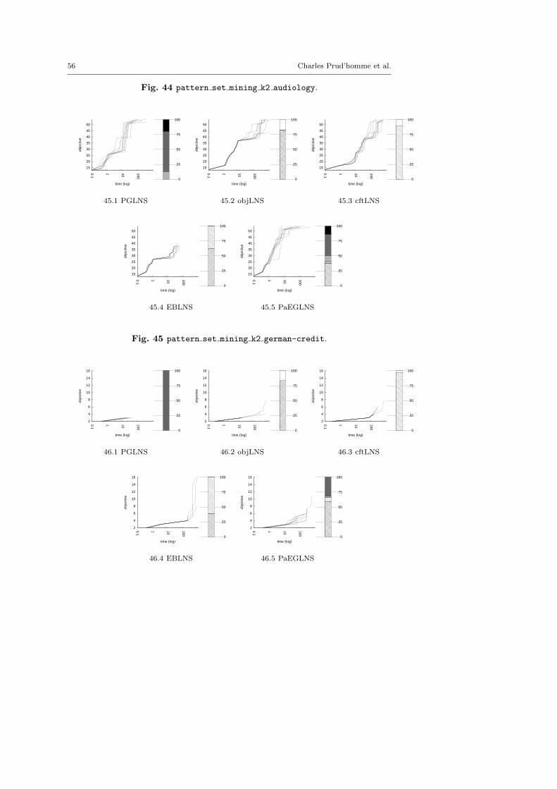
56 Charles Prud’homme et al.
Fig. 44 pattern set mining k2 audiology.
15
20
25
30
35
40
45
50
0.1
1 10
100
obje
ctiv
e
time (log) 0
25
50
75
100
45.1 PGLNS
15
20
25
30
35
40
45
50
0.1
1 10
100
obje
ctiv
e
time (log) 0
25
50
75
100
45.2 objLNS
15
20
25
30
35
40
45
50
0.1
1 10
100
obje
ctiv
e
time (log) 0
25
50
75
100
45.3 cftLNS
15
20
25
30
35
40
45
50
0.1
1 10
100
obje
ctiv
e
time (log) 0
25
50
75
100
45.4 EBLNS
15
20
25
30
35
40
45
50
0.1
1 10
100
obje
ctiv
e
time (log) 0
25
50
75
100
45.5 PaEGLNS
Fig. 45 pattern set mining k2 german-credit.
2
4
6
8
10
12
14
16
0.1
1 10
100
obje
ctiv
e
time (log) 0
25
50
75
100
46.1 PGLNS
2
4
6
8
10
12
14
16
0.1
1 10
100
obje
ctiv
e
time (log) 0
25
50
75
100
46.2 objLNS
2
4
6
8
10
12
14
16
0.1
1 10
100
obje
ctiv
e
time (log) 0
25
50
75
100
46.3 cftLNS
2
4
6
8
10
12
14
16
0.1
1 10
100
obje
ctiv
e
time (log) 0
25
50
75
100
46.4 EBLNS
2
4
6
8
10
12
14
16
0.1
1 10
100
obje
ctiv
e
time (log) 0
25
50
75
100
46.5 PaEGLNS
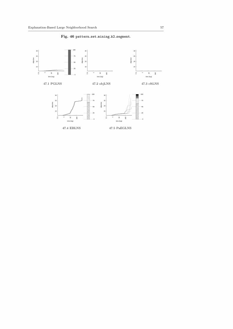
Explanation-Based Large Neighborhood Search 57
Fig. 46 pattern set mining k2 segment.
15
20
25
30
0.1
1 10
100
obje
ctiv
e
time (log) 0
25
50
75
100
47.1 PGLNS
15
20
25
30
0.1
1 10
100
obje
ctiv
e
time (log)
47.2 objLNS
15
20
25
30
0.1
1 10
100
obje
ctiv
e
time (log)
47.3 cftLNS
15
20
25
30
0.1
1 10
100
obje
ctiv
e
time (log) 0
25
50
75
100
47.4 EBLNS
15
20
25
30
0.1
1 10
100
obje
ctiv
e
time (log) 0
25
50
75
100
47.5 PaEGLNS
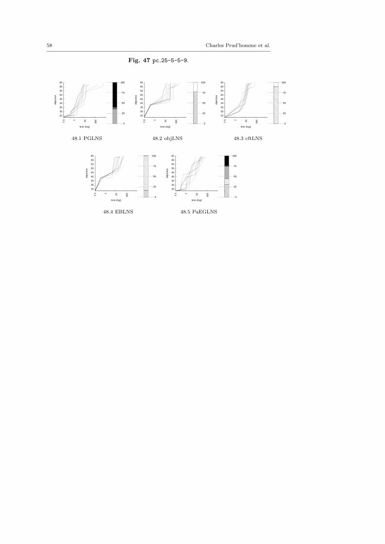
58 Charles Prud’homme et al.
Fig. 47 pc 25-5-5-9.
25
30
35
40
45
50
55
60
65
0.1
1 10
100
obje
ctiv
e
time (log) 0
25
50
75
100
48.1 PGLNS
25
30
35
40
45
50
55
60
65
0.1
1 10
100
obje
ctiv
e
time (log) 0
25
50
75
100
48.2 objLNS
25
30
35
40
45
50
55
60
65
0.1
1 10
100
obje
ctiv
e
time (log) 0
25
50
75
100
48.3 cftLNS
25
30
35
40
45
50
55
60
65
0.1
1 10
100
obje
ctiv
e
time (log) 0
25
50
75
100
48.4 EBLNS
25
30
35
40
45
50
55
60
65
0.1
1 10
100
obje
ctiv
e
time (log) 0
25
50
75
100
48.5 PaEGLNS
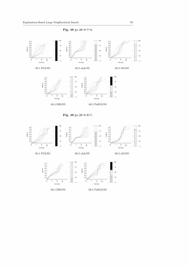
Explanation-Based Large Neighborhood Search 59
Fig. 48 pc 28-4-7-4.
15
20
25
30
35
40
45
50
55
0.1
1 10
100
obje
ctiv
e
time (log) 0
25
50
75
100
49.1 PGLNS
15
20
25
30
35
40
45
50
55
0.1
1 10
100
obje
ctiv
e
time (log) 0
25
50
75
100
49.2 objLNS
15
20
25
30
35
40
45
50
55
0.1
1 10
100
obje
ctiv
e
time (log) 0
25
50
75
100
49.3 cftLNS
15
20
25
30
35
40
45
50
55
0.1
1 10
100
obje
ctiv
e
time (log) 0
25
50
75
100
49.4 EBLNS
15
20
25
30
35
40
45
50
55
0.1
1 10
100
obje
ctiv
e
time (log) 0
25
50
75
100
49.5 PaEGLNS
Fig. 49 pc 30-5-6-7.
30
35
40
45
50
55
60
0.1
1 10
100
obje
ctiv
e
time (log) 0
25
50
75
100
50.1 PGLNS
30
35
40
45
50
55
60
0.1
1 10
100
obje
ctiv
e
time (log) 0
25
50
75
100
50.2 objLNS
30
35
40
45
50
55
60
0.1
1 10
100
obje
ctiv
e
time (log) 0
25
50
75
100
50.3 cftLNS
30
35
40
45
50
55
60
0.1
1 10
100
obje
ctiv
e
time (log) 0
25
50
75
100
50.4 EBLNS
30
35
40
45
50
55
60
0.1
1 10
100
obje
ctiv
e
time (log) 0
25
50
75
100
50.5 PaEGLNS
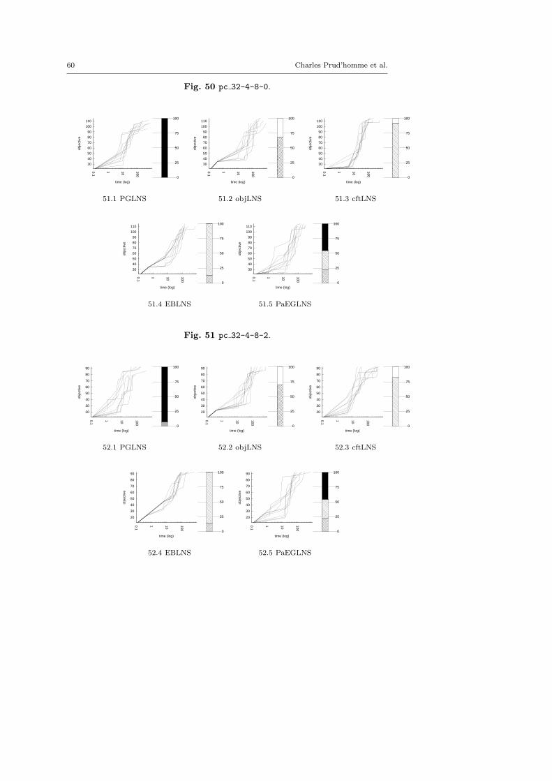
60 Charles Prud’homme et al.
Fig. 50 pc 32-4-8-0.
30
40
50
60
70
80
90
100
110
0.1
1 10
100
obje
ctiv
e
time (log) 0
25
50
75
100
51.1 PGLNS
30
40
50
60
70
80
90
100
110
0.1
1 10
100
obje
ctiv
e
time (log) 0
25
50
75
100
51.2 objLNS
30
40
50
60
70
80
90
100
110
0.1
1 10
100
obje
ctiv
e
time (log) 0
25
50
75
100
51.3 cftLNS
30
40
50
60
70
80
90
100
110
0.1
1 10
100
obje
ctiv
e
time (log) 0
25
50
75
100
51.4 EBLNS
30
40
50
60
70
80
90
100
110
0.1
1 10
100
obje
ctiv
e
time (log) 0
25
50
75
100
51.5 PaEGLNS
Fig. 51 pc 32-4-8-2.
20
30
40
50
60
70
80
90
0.1
1 10
100
obje
ctiv
e
time (log) 0
25
50
75
100
52.1 PGLNS
20
30
40
50
60
70
80
90
0.1
1 10
100
obje
ctiv
e
time (log) 0
25
50
75
100
52.2 objLNS
20
30
40
50
60
70
80
90
0.1
1 10
100
obje
ctiv
e
time (log) 0
25
50
75
100
52.3 cftLNS
20
30
40
50
60
70
80
90
0.1
1 10
100
obje
ctiv
e
time (log) 0
25
50
75
100
52.4 EBLNS
20
30
40
50
60
70
80
90
0.1
1 10
100
obje
ctiv
e
time (log) 0
25
50
75
100
52.5 PaEGLNS
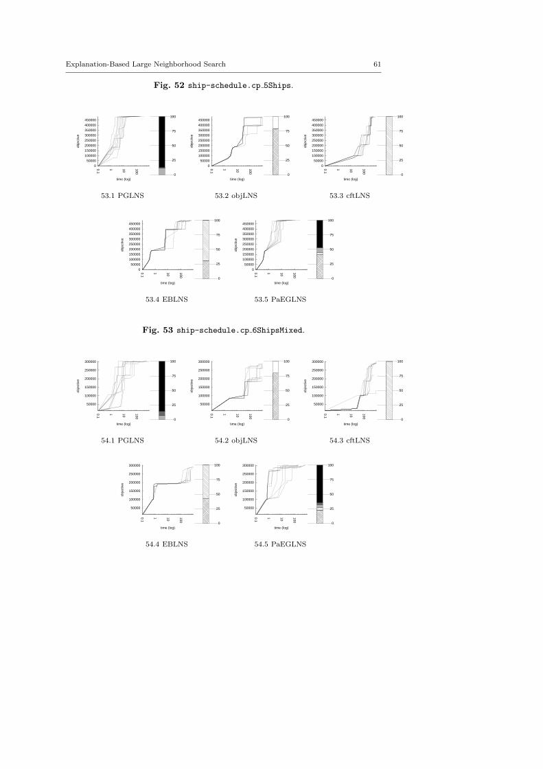
Explanation-Based Large Neighborhood Search 61
Fig. 52 ship-schedule.cp 5Ships.
0
50000
100000
150000
200000
250000
300000
350000
400000
450000
0.1
1 10
100
obje
ctiv
e
time (log) 0
25
50
75
100
53.1 PGLNS
0
50000
100000
150000
200000
250000
300000
350000
400000
450000
0.1
1 10
100
obje
ctiv
e
time (log) 0
25
50
75
100
53.2 objLNS
0
50000
100000
150000
200000
250000
300000
350000
400000
450000
0.1
1 10
100
obje
ctiv
e
time (log) 0
25
50
75
100
53.3 cftLNS
0
50000
100000
150000
200000
250000
300000
350000
400000
450000
0.1
1 10
100
obje
ctiv
e
time (log) 0
25
50
75
100
53.4 EBLNS
0
50000
100000
150000
200000
250000
300000
350000
400000
450000
0.1
1 10
100
obje
ctiv
e
time (log) 0
25
50
75
100
53.5 PaEGLNS
Fig. 53 ship-schedule.cp 6ShipsMixed.
50000
100000
150000
200000
250000
300000
0.1
1 10
100
obje
ctiv
e
time (log) 0
25
50
75
100
54.1 PGLNS
50000
100000
150000
200000
250000
300000
0.1
1 10
100
obje
ctiv
e
time (log) 0
25
50
75
100
54.2 objLNS
50000
100000
150000
200000
250000
300000
0.1
1 10
100
obje
ctiv
e
time (log) 0
25
50
75
100
54.3 cftLNS
50000
100000
150000
200000
250000
300000
0.1
1 10
100
obje
ctiv
e
time (log) 0
25
50
75
100
54.4 EBLNS
50000
100000
150000
200000
250000
300000
0.1
1 10
100
obje
ctiv
e
time (log) 0
25
50
75
100
54.5 PaEGLNS

62 Charles Prud’homme et al.
Fig. 54 ship-schedule.cp 7ShipsMixed.
50000
100000
150000
200000
250000
300000
350000
400000
0.1
1 10
100
obje
ctiv
e
time (log) 0
25
50
75
100
55.1 PGLNS
50000
100000
150000
200000
250000
300000
350000
400000
0.1
1 10
100
obje
ctiv
e
time (log) 0
25
50
75
100
55.2 objLNS
50000
100000
150000
200000
250000
300000
350000
400000
0.1
1 10
100
obje
ctiv
e
time (log) 0
25
50
75
100
55.3 cftLNS
50000
100000
150000
200000
250000
300000
350000
400000
0.1
1 10
100
obje
ctiv
e
time (log) 0
25
50
75
100
55.4 EBLNS
50000
100000
150000
200000
250000
300000
350000
400000
0.1
1 10
100
obje
ctiv
e
time (log) 0
25
50
75
100
55.5 PaEGLNS
Fig. 55 ship-schedule.cp 7ShipsMixedUnconst.
50000
100000
150000
200000
250000
300000
350000
0.1
1 10
100
obje
ctiv
e
time (log) 0
25
50
75
100
56.1 PGLNS
50000
100000
150000
200000
250000
300000
350000
0.1
1 10
100
obje
ctiv
e
time (log) 0
25
50
75
100
56.2 objLNS
50000
100000
150000
200000
250000
300000
350000
0.1
1 10
100
obje
ctiv
e
time (log) 0
25
50
75
100
56.3 cftLNS
50000
100000
150000
200000
250000
300000
350000
0.1
1 10
100
obje
ctiv
e
time (log) 0
25
50
75
100
56.4 EBLNS
50000
100000
150000
200000
250000
300000
350000
0.1
1 10
100
obje
ctiv
e
time (log) 0
25
50
75
100
56.5 PaEGLNS
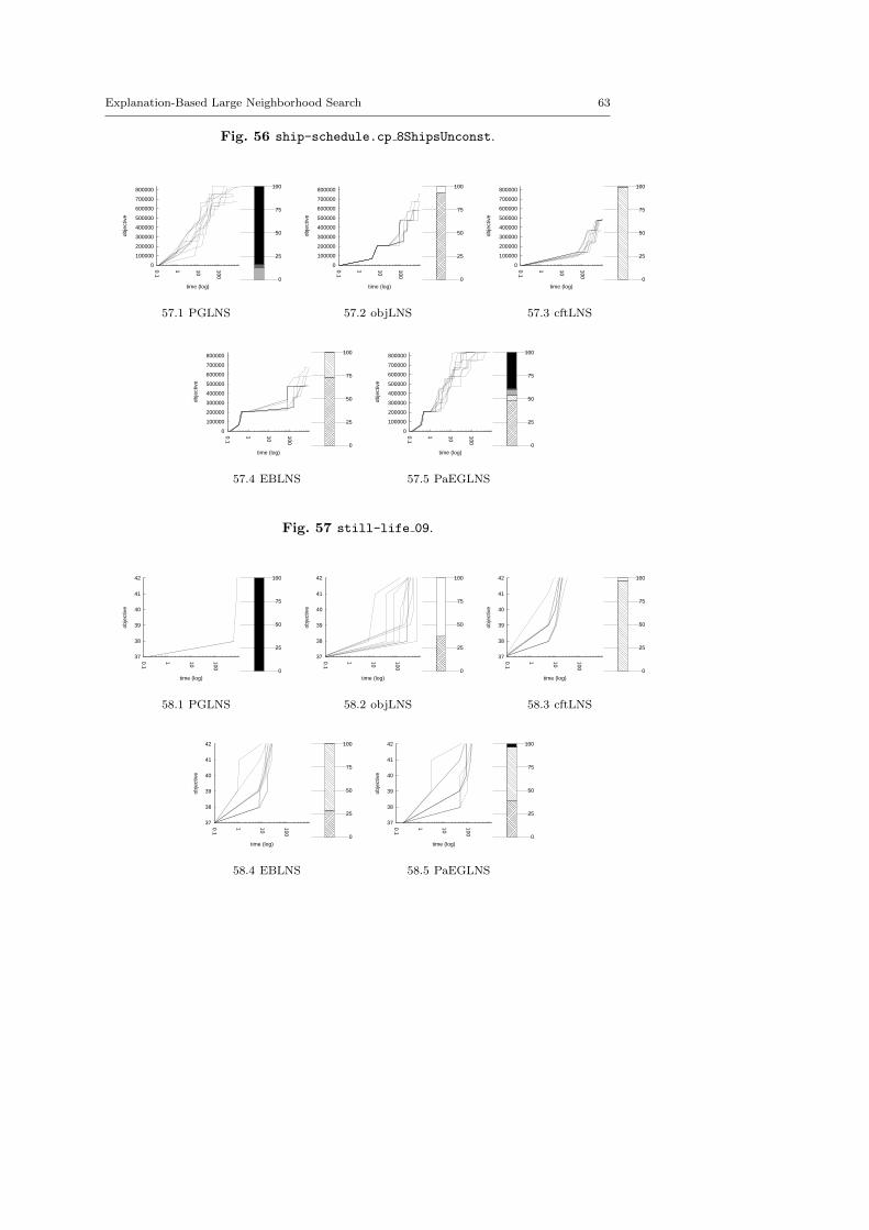
Explanation-Based Large Neighborhood Search 63
Fig. 56 ship-schedule.cp 8ShipsUnconst.
0
100000
200000
300000
400000
500000
600000
700000
800000
0.1
1 10
100
obje
ctiv
e
time (log) 0
25
50
75
100
57.1 PGLNS
0
100000
200000
300000
400000
500000
600000
700000
800000
0.1
1 10
100
obje
ctiv
e
time (log) 0
25
50
75
100
57.2 objLNS
0
100000
200000
300000
400000
500000
600000
700000
800000
0.1
1 10
100
obje
ctiv
e
time (log) 0
25
50
75
100
57.3 cftLNS
0
100000
200000
300000
400000
500000
600000
700000
800000
0.1
1 10
100
obje
ctiv
e
time (log) 0
25
50
75
100
57.4 EBLNS
0
100000
200000
300000
400000
500000
600000
700000
800000
0.1
1 10
100
obje
ctiv
e
time (log) 0
25
50
75
100
57.5 PaEGLNS
Fig. 57 still-life 09.
37
38
39
40
41
42
0.1
1 10
100
obje
ctiv
e
time (log) 0
25
50
75
100
58.1 PGLNS
37
38
39
40
41
42
0.1
1 10
100
obje
ctiv
e
time (log) 0
25
50
75
100
58.2 objLNS
37
38
39
40
41
42
0.1
1 10
100
obje
ctiv
e
time (log) 0
25
50
75
100
58.3 cftLNS
37
38
39
40
41
42
0.1
1 10
100
obje
ctiv
e
time (log) 0
25
50
75
100
58.4 EBLNS
37
38
39
40
41
42
0.1
1 10
100
obje
ctiv
e
time (log) 0
25
50
75
100
58.5 PaEGLNS

64 Charles Prud’homme et al.
Fig. 58 still-life 10.
47
48
49
50
51
52
53
54
0.1
1 10
100
obje
ctiv
e
time (log) 0
25
50
75
100
59.1 PGLNS
47
48
49
50
51
52
53
54
0.1
1 10
100
obje
ctiv
e
time (log) 0
25
50
75
100
59.2 objLNS
47
48
49
50
51
52
53
54
0.1
1 10
100
obje
ctiv
e
time (log) 0
25
50
75
100
59.3 cftLNS
47
48
49
50
51
52
53
54
0.1
1 10
100
obje
ctiv
e
time (log) 0
25
50
75
100
59.4 EBLNS
47
48
49
50
51
52
53
54
0.1
1 10
100
obje
ctiv
e
time (log) 0
25
50
75
100
59.5 PaEGLNS
Fig. 59 still-life 11.
58
58.5
59
59.5
60
60.5
61
61.5
62
0.1
1 10
100
obje
ctiv
e
time (log) 0
25
50
75
100
60.1 PGLNS
58
58.5
59
59.5
60
60.5
61
61.5
62
0.1
1 10
100
obje
ctiv
e
time (log) 0
25
50
75
100
60.2 objLNS
58
58.5
59
59.5
60
60.5
61
61.5
62
0.1
1 10
100
obje
ctiv
e
time (log) 0
25
50
75
100
60.3 cftLNS
58
58.5
59
59.5
60
60.5
61
61.5
62
0.1
1 10
100
obje
ctiv
e
time (log) 0
25
50
75
100
60.4 EBLNS
58
58.5
59
59.5
60
60.5
61
61.5
62
0.1
1 10
100
obje
ctiv
e
time (log) 0
25
50
75
100
60.5 PaEGLNS
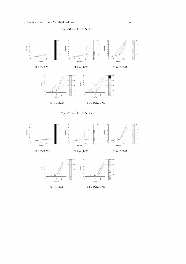
Explanation-Based Large Neighborhood Search 65
Fig. 60 still-life 12.
62
64
66
68
70
72
74
76
0.1
1 10
100
obje
ctiv
e
time (log) 0
25
50
75
100
61.1 PGLNS
62
64
66
68
70
72
74
76
0.1
1 10
100
obje
ctiv
e
time (log) 0
25
50
75
100
61.2 objLNS
62
64
66
68
70
72
74
76
0.1
1 10
100
obje
ctiv
e
time (log) 0
25
50
75
100
61.3 cftLNS
62
64
66
68
70
72
74
76
0.1
1 10
100
obje
ctiv
e
time (log) 0
25
50
75
100
61.4 EBLNS
62
64
66
68
70
72
74
76
0.1
1 10
100
obje
ctiv
e
time (log) 0
25
50
75
100
61.5 PaEGLNS
Fig. 61 still-life 13.
78
80
82
84
86
88
0.1
1 10
100
obje
ctiv
e
time (log) 0
25
50
75
100
62.1 PGLNS
78
80
82
84
86
88
0.1
1 10
100
obje
ctiv
e
time (log) 0
25
50
75
100
62.2 objLNS
78
80
82
84
86
88
0.1
1 10
100
obje
ctiv
e
time (log) 0
25
50
75
100
62.3 cftLNS
78
80
82
84
86
88
0.1
1 10
100
obje
ctiv
e
time (log) 0
25
50
75
100
62.4 EBLNS
78
80
82
84
86
88
0.1
1 10
100
obje
ctiv
e
time (log) 0
25
50
75
100
62.5 PaEGLNS