Explaining Wide Area Data Transfer Performancekettimut/publications/hpdc17-final.pdfExplaining Wide Area Data Transfer Performance Zhengchun Liu Argonne National Laboratory Lemont,

Explaining Wide Area Data Transfer PerformanceZhengchun Liu

Argonne National LaboratoryLemont, IL, USA

[email protected]

Prasanna BalaprakashArgonne National Laboratory

Lemont, IL, [email protected]

Rajkumar Ke�imuthuArgonne National Laboratory

Lemont, IL, USAke�[email protected]

Ian FosterArgonne National Lab and University of Chicago

Lemont, IL, [email protected]

ABSTRACTDisk-to-disk wide-area �le transfers involve many subsystems andtunable application parameters that pose signi�cant challengesfor bo�leneck detection, system optimization, and performanceprediction. Performance models can be used to address these chal-lenges but have not proved generally usable because of a need forextensive online experiments to characterize subsystems. We showhere how to overcome the need for such experiments by applyingmachine learning methods to historical data to estimate parametersfor predictive models. Starting with log data for millions of Globustransfers involving billions of �les and hundreds of petabytes, weengineer features for endpoint CPU load, network interface cardload, and transfer characteristics; and we use these features in bothlinear and nonlinear models of transfer performance, We show thatthe resulting models have high explanatory power. For a represen-tative set of 30,653 transfers over 30 heavily used source-destinationpairs (“edges”), totaling 2,053 TB in 46.6 million �les, we obtainmedian absolute percentage prediction errors (MdAPE) of 7.0% and4.6% when using distinct linear and nonlinear models per edge,respectively; when using a single nonlinear model for all edges, weobtain an MdAPE of 7.8%. Our work broadens understanding offactors that in�uence �le transfer rate by clarifying relationshipsbetween achieved transfer rates, transfer characteristics, and com-peting load. Our predictions can be used for distributed work�owscheduling and optimization, and our features can also be used foroptimization and explanation.

1 INTRODUCTIONMany researchers have studied the performance of network archi-tectures, storage systems, protocols, and tools for high-speed �letransfer [15, 20, 25, 33, 36, 38]. Using a mix of experiment, modeling,and simulation, o�en in highly controlled environments, this workhas produced a good understanding of how, in principle, to con�g-ure hardware and so�ware systems in order to enable extremely

Publication rights licensed to ACM. ACM acknowledges that this contribution wasauthored or co-authored by an employee, contractor or a�liate of the United Statesgovernment. As such, the Government retains a nonexclusive, royalty-free right topublish or reproduce this article, or to allow others to do so, for Government purposesonly.HPDC ’17, June 26-30, 2017, Washington, DC, USA© 2017 Copyright held by the owner/author(s). Publication rights licensed to ACM.978-1-4503-4699-3/17/06. . .$15.00DOI: h�p://dx.doi.org/10.1145/3078597.3078605

high-speed transfers, which can achieve close to line rates on 10Gbps and even 100 Gbps networks [11, 23].

Yet despite these results, the actual performance achieved bydisk-to-disk transfers in practical se�ings is usually much lowerthan line rates. For example, a study of more than 3.9 million Globustransfers [8] involving more than 33 billion �les and 223 PB over aseven-year period (2010-2016) shows an average transfer speed ofonly 11.5 MB/s. (On the other hand, 52% of all bytes moved overthat period moved at >100 MB/s and 14% moved at >1 GB/s.)

With e�ort, we can o�en explain each low-performing trans-fer, which may result from (mis)con�gurations and/or interactionsamong storage devices, �le systems, CPUs, operating systems, net-work interfaces, intermediate network devices, local and wide areanetworks, �le transfer so�ware, network protocols, and competingactivities. But we have lacked an approach that could use easilyobtainable information sources to explain and improve the per-formance of arbitrary transfers in arbitrary environments. Webelieve that lightweight models are required for this purpose andthat the construction of such models will require a combinationof data-driven analysis of large collections of historical data, thedevelopment and testing of expressive analytical models of variousaspects of transfer performance, and new data sources. Here wereport on steps toward this goal.

�is paper makes four contributions. (1) We show how to usemachine learning methods to develop data transfer performancemodels using only historical data. (2) We engineer features for usein these models, including features that characterize competingload at source and destination endpoints. (3) We identify featuresthat have nonlinear impact on transfer performance, in particularthose that capture competing load. (4) We demonstrate that modelaccuracy can be improved even further by using new data sourcesto obtain more complete knowledge of competing load.

�e rest of the paper is organized as follows. In §2 we providebackground on the Globus service that manages the transfers con-sidered here. In §3 we introduce a simple three-feature analyticalmodel that provides just an upper bound on performance, and weuse this model to identify factors that impact maximum achievabletransfer rate. In §4 we analyze additional factors that a�ect transferrate, and we de�ne the features that we use in the data-drivenmodels we introduce in §5, where we describe and evaluate bothlinear and nonlinear regression models. Starting from a di�erentmodel for each edge, we incorporate endpoint- and edge-speci�cfeatures to develop one model for all edges. In §6 we review related

Performance Modeling and Analysis HPDC'17, June 26–30, 2017, Washington, DC, USA

167

Storage System

GridFTP

Network

Storage System

GridFTP

Network

Endpoint 1 Endpoint 2

WAN

disk-to-disk

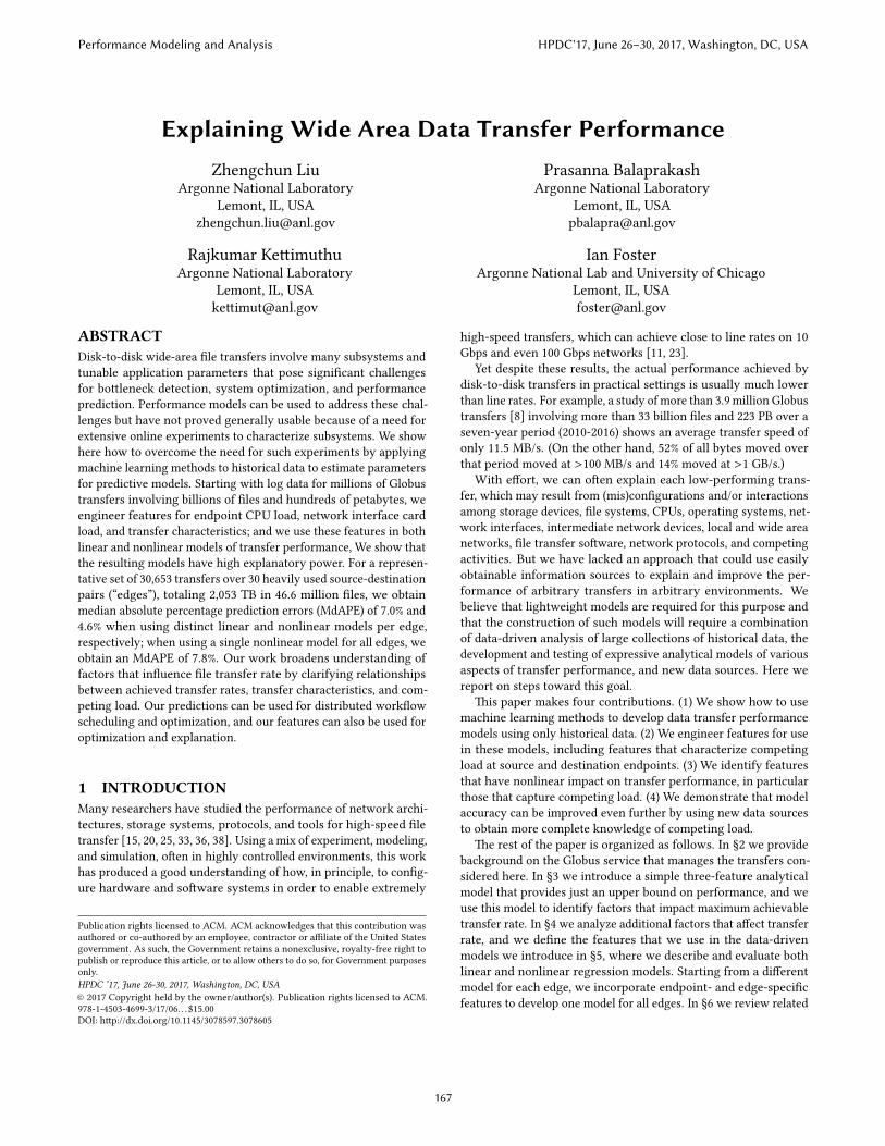
Figure 1: Structure of a Globus end-to-end �le transfer fromsource (le�) to destination (right), managed by cloud service.

work, in §7 discuss the broader applicability of our work, and in §8summarize our conclusions and brie�y discuss future work.

2 BACKGROUND ON THE GLOBUS SERVICE�e Globus transfer service is a cloud-hosted so�ware-as-a-serviceimplementation of the logic required to orchestrate �le transfersbetween pairs of storage systems [2] (see Figure 1). A transferrequest speci�es, among other things, a source and destination; the�les and/or directories to be transferred; and (optionally) whetherto perform integrity checking (enabled by default) and/or to encryptthe data (disabled by default). Globus can transfer data with eitherthe GridFTP or HTTP protocol; we focus here on GridFTP transfers,since HTTP support has been added only recently. GridFTP extendsFTP with features required for speed, reliability, and security.

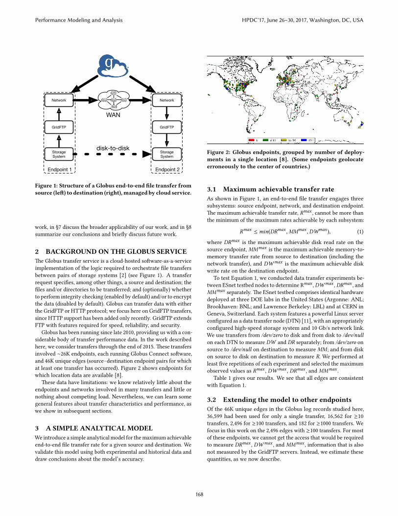
Globus has been running since late 2010, providing us with a con-siderable body of transfer performance data. In the work describedhere, we consider transfers through the end of 2015. �ese transfersinvolved ∼26K endpoints, each running Globus Connect so�ware,and 46K unique edges (source–destination endpoint pairs for whichat least one transfer has occurred). Figure 2 shows endpoints forwhich location data are available [8].

�ese data have limitations: we know relatively li�le about theendpoints and networks involved in many transfers and li�le ornothing about competing load. Nevertheless, we can learn somegeneral features about transfer characteristics and performance, aswe show in subsequent sections.

3 A SIMPLE ANALYTICAL MODELWe introduce a simple analytical model for themaximum achievableend-to-end �le transfer rate for a given source and destination. Wevalidate this model using both experimental and historical data anddraw conclusions about the model’s accuracy.

Figure 2: Globus endpoints, grouped by number of deploy-ments in a single location [8]. (Some endpoints geolocateerroneously to the center of countries.)

3.1 Maximum achievable transfer rateAs shown in Figure 1, an end-to-end �le transfer engages threesubsystems: source endpoint, network, and destination endpoint.�e maximum achievable transfer rate, Rmax , cannot be more thanthe minimum of the maximum rates achievable by each subsystem:

Rmax ≤ min(DRmax ,MMmax ,DWmax ), (1)

where DRmax is the maximum achievable disk read rate on thesource endpoint, MMmax is the maximum achievable memory-to-memory transfer rate from source to destination (including thenetwork transfer), and DWmax is the maximum achievable diskwrite rate on the destination endpoint.

To test Equation 1, we conducted data transfer experiments be-tween ESnet testbed nodes to determine Rmax , DWmax , DRmax , andMMmax separately. �e ESnet testbed comprises identical hardwaredeployed at three DOE labs in the United States (Argonne: ANL;Brookhaven: BNL; and Lawrence Berkeley: LBL) and at CERN inGeneva, Switzerland. Each system features a powerful Linux servercon�gured as a data transfer node (DTN) [11], with an appropriatelycon�gured high-speed storage system and 10 Gb/s network link.We use transfers from /dev/zero to disk and from disk to /dev/nullon each DTN to measure DW and DR separately; from /dev/zero onsource to /dev/null on destination to measure MM; and from diskon source to disk on destination to measure R. We performed atleast �ve repetitions of each experiment and selected the maximumobserved values as Rmax , DWmax , DRmax , and MMmax .

Table 1 gives our results. We see that all edges are consistentwith Equation 1.

3.2 Extending the model to other endpointsOf the 46K unique edges in the Globus log records studied here,36,599 had been used for only a single transfer, 16,562 for ≥10transfers, 2,496 for ≥100 transfers, and 182 for ≥1000 transfers. Wefocus in this work on the 2,496 edges with ≥100 transfers. For mostof these endpoints, we cannot get the access that would be requiredto measure DRmax , DWmax , and MMmax , information that is alsonot measured by the GridFTP servers. Instead, we estimate thesequantities, as we now describe.


168

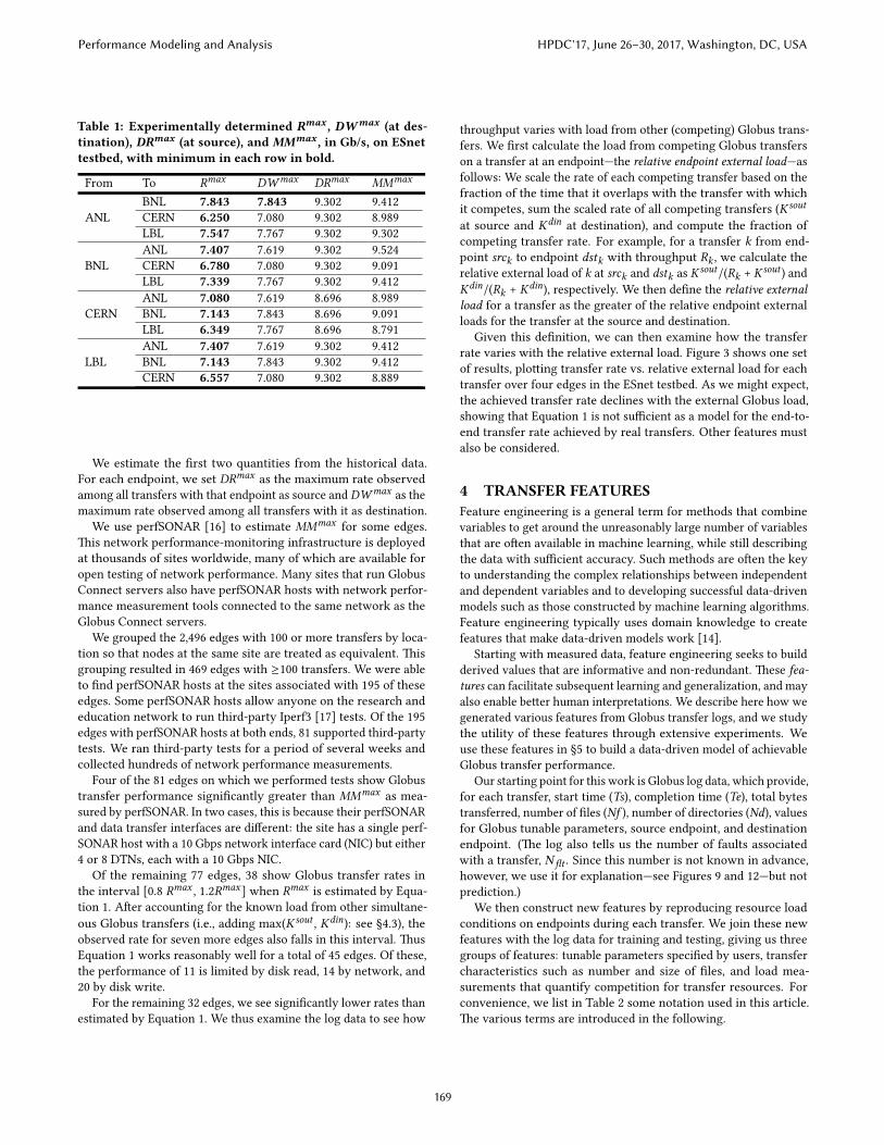
Table 1: Experimentally determined Rmax , DWmax (at des-tination), DRmax (at source), and MMmax , in Gb/s, on ESnettestbed, with minimum in each row in bold.

From To Rmax DWmax DRmax MMmax

ANLBNL 7.843 7.843 9.302 9.412CERN 6.250 7.080 9.302 8.989LBL 7.547 7.767 9.302 9.302

BNLANL 7.407 7.619 9.302 9.524CERN 6.780 7.080 9.302 9.091LBL 7.339 7.767 9.302 9.412

CERNANL 7.080 7.619 8.696 8.989BNL 7.143 7.843 8.696 9.091LBL 6.349 7.767 8.696 8.791

LBLANL 7.407 7.619 9.302 9.412BNL 7.143 7.843 9.302 9.412CERN 6.557 7.080 9.302 8.889

We estimate the �rst two quantities from the historical data.For each endpoint, we set DRmax as the maximum rate observedamong all transfers with that endpoint as source and DWmax as themaximum rate observed among all transfers with it as destination.

We use perfSONAR [16] to estimate MMmax for some edges.�is network performance-monitoring infrastructure is deployedat thousands of sites worldwide, many of which are available foropen testing of network performance. Many sites that run GlobusConnect servers also have perfSONAR hosts with network perfor-mance measurement tools connected to the same network as theGlobus Connect servers.

We grouped the 2,496 edges with 100 or more transfers by loca-tion so that nodes at the same site are treated as equivalent. �isgrouping resulted in 469 edges with ≥100 transfers. We were ableto �nd perfSONAR hosts at the sites associated with 195 of theseedges. Some perfSONAR hosts allow anyone on the research andeducation network to run third-party Iperf3 [17] tests. Of the 195edges with perfSONAR hosts at both ends, 81 supported third-partytests. We ran third-party tests for a period of several weeks andcollected hundreds of network performance measurements.

Four of the 81 edges on which we performed tests show Globustransfer performance signi�cantly greater than MMmax as mea-sured by perfSONAR. In two cases, this is because their perfSONARand data transfer interfaces are di�erent: the site has a single perf-SONAR host with a 10 Gbps network interface card (NIC) but either4 or 8 DTNs, each with a 10 Gbps NIC.

Of the remaining 77 edges, 38 show Globus transfer rates inthe interval [0.8 Rmax , 1.2Rmax] when Rmax is estimated by Equa-tion 1. A�er accounting for the known load from other simultane-ous Globus transfers (i.e., adding max(K sout , Kdin): see §4.3), theobserved rate for seven more edges also falls in this interval. �usEquation 1 works reasonably well for a total of 45 edges. Of these,the performance of 11 is limited by disk read, 14 by network, and20 by disk write.

For the remaining 32 edges, we see signi�cantly lower rates thanestimated by Equation 1. We thus examine the log data to see how

throughput varies with load from other (competing) Globus trans-fers. We �rst calculate the load from competing Globus transferson a transfer at an endpoint—the relative endpoint external load—asfollows: We scale the rate of each competing transfer based on thefraction of the time that it overlaps with the transfer with whichit competes, sum the scaled rate of all competing transfers (Ksout

at source and Kdin at destination), and compute the fraction ofcompeting transfer rate. For example, for a transfer k from end-point srck to endpoint dstk with throughput Rk , we calculate therelative external load of k at srck and dstk as Ksout/(Rk + Ksout ) andKdin/(Rk + Kdin), respectively. We then de�ne the relative externalload for a transfer as the greater of the relative endpoint externalloads for the transfer at the source and destination.

Given this de�nition, we can then examine how the transferrate varies with the relative external load. Figure 3 shows one setof results, plo�ing transfer rate vs. relative external load for eachtransfer over four edges in the ESnet testbed. As we might expect,the achieved transfer rate declines with the external Globus load,showing that Equation 1 is not su�cient as a model for the end-to-end transfer rate achieved by real transfers. Other features mustalso be considered.

4 TRANSFER FEATURESFeature engineering is a general term for methods that combinevariables to get around the unreasonably large number of variablesthat are o�en available in machine learning, while still describingthe data with su�cient accuracy. Such methods are o�en the keyto understanding the complex relationships between independentand dependent variables and to developing successful data-drivenmodels such as those constructed by machine learning algorithms.Feature engineering typically uses domain knowledge to createfeatures that make data-driven models work [14].

Starting with measured data, feature engineering seeks to buildderived values that are informative and non-redundant. �ese fea-tures can facilitate subsequent learning and generalization, and mayalso enable be�er human interpretations. We describe here how wegenerated various features from Globus transfer logs, and we studythe utility of these features through extensive experiments. Weuse these features in §5 to build a data-driven model of achievableGlobus transfer performance.

Our starting point for this work is Globus log data, which provide,for each transfer, start time (Ts), completion time (Te), total bytestransferred, number of �les (Nf ), number of directories (Nd), valuesfor Globus tunable parameters, source endpoint, and destinationendpoint. (�e log also tells us the number of faults associatedwith a transfer, N�t . Since this number is not known in advance,however, we use it for explanation—see Figures 9 and 12—but notprediction.)

We then construct new features by reproducing resource loadconditions on endpoints during each transfer. We join these newfeatures with the log data for training and testing, giving us threegroups of features: tunable parameters speci�ed by users, transfercharacteristics such as number and size of �les, and load mea-surements that quantify competition for transfer resources. Forconvenience, we list in Table 2 some notation used in this article.�e various terms are introduced in the following.


169

0.0 0.2 0.4 0.6 0.8 1.0Relative external load

0

200

400

600

800

1000

1200

1400

Tran

sfer

rate

(MB/

s)

max rate transfer

(a) ANL to BNL


0

200

400

600

800

1000

1200

1400

Tran

sfer

rate

(MB/

s)

max rate transfer

(b) CERN to BNL


0

200

400

600

800

1000

1200

1400

Tran

sfer

rate

(MB/

s)

max rate transfer

(c) BNL to LBL


0

200

400

600

800

1000

1200

1400

Tran

sfer

rate

(MB/

s)

max rate transfer

(d) CERN to ANL

Figure 3: Transfer rate vs. relative external load: ESnet.

4.1 Tunable parameters�e Globus GridFTP implementation includes user-con�gurablefeatures that can be used to optimize transfer performance [1]. Twothat are commonly used are concurrency (C) and parallelism (P ).Concurrency involves starting C independent GridFTP processesat the source and destination endpoints. Each of the resultingC process pairs can then work on the transfer of a separate �le,thus providing for concurrency at the �le system I/O, CPU core,and network levels. In general, concurrency is good for multi-�le transfers, since it can drive more �lesystem processes, CPUcores, and even endpoint servers, in addition to opening more TCPstreams. Parallelism is a network-level optimization, in which datablocks for a single �le between a process pair are distributed overP TCP streams. Large �les over high-latency links can bene�t fromhigher parallelism, for reasons noted in §6.

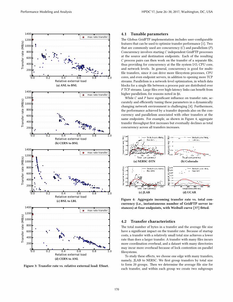
While C and P have signi�cant in�uence on transfer rate, ac-curately and e�ciently tuning these parameters in a dynamicallychanging network environment is challenging [4]. Furthermore,the performance achieved by a transfer depends also on the con-currency and parallelism associated with other transfers at thesame endpoints. For example, as shown in Figure 4, aggregatetransfer throughput �rst increases but eventually declines as totalconcurrency across all transfers increases.

(a) NERSC-DTN (b) Colorado

(c) JLAB (d) UCAR

Figure 4: Aggregate incoming transfer rate vs. total con-currency (i.e., instantaneous number of GridFTP server in-stances) at four endpoints, with Weibull curve [37] �tted.

4.2 Transfer characteristics�e total number of bytes in a transfer and the average �le sizehave a signi�cant impact on the transfer rate. Because of startupcosts, a transfer with a relatively small total size achieves a lowerrate than does a larger transfer. A transfer with many �les incursmore coordination overhead, and a dataset with many directoriesmay incur more overhead because of lock contention on parallel�lesystems.

To study these e�ects, we choose one edge with many transfers,namely, JLAB to NERSC. We �rst group transfers by total sizeto form 20 groups. �en we determine the average �le size foreach transfer, and within each group we create two subgroups


170

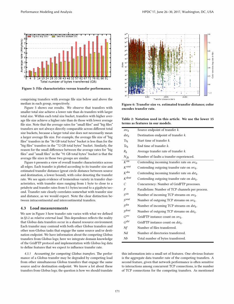
Figure 5: File characteristics versus transfer performance.

comprising transfers with average �le size below and above themedian in each group, respectively.

Figure 5 shows our results. We observe that transfers withsmaller total size achieve a lower rate than do transfers with largertotal size. Within each total size bucket, transfers with higher aver-age �le size achieve a higher rate than do those with lower average�le size. Note that the average rates for “small �les” and “big �les”transfers are not always directly comparable across di�erent totalsize buckets, because a larger total size does not necessarily meana larger average �le size. For example, the average �le size of “big�les” transfers in the “86 GB total bytes” bucket is less than for the“big �les” transfers in the “72 GB total bytes” bucket. Similarly, thereason for the small di�erence between the average rates for “big�les” and “small �les” in the “91 GB total bytes” bucket is that theaverage �le sizes in those two groups are similar.

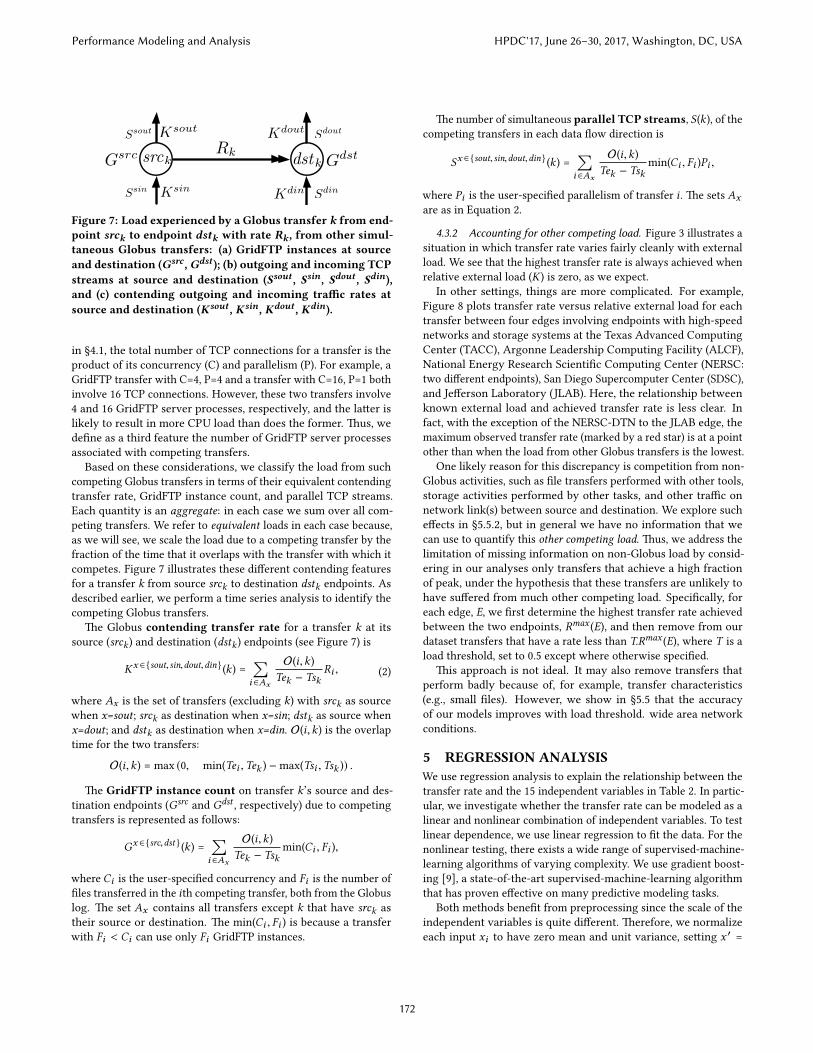
Figure 6 presents a view of overall transfer characteristics acrossall edges. Each transfer is plo�ed according to its transfer size andestimated transfer distance (great circle distance between sourceand destination, a lower bound), with color denoting the transferrate. We see again evidence of tremendous variety in transfer char-acteristics, with transfer sizes ranging from 1 byte to close to apetabyte and transfer rates from 0.1 bytes/second to a gigabyte/sec-ond. Transfer rate clearly correlates somewhat with transfer sizeand distance, as we would expect. Note the clear distinction be-tween intracontinental and intercontinental transfers.

4.3 Load measurementsWe saw in Figure 3 how transfer rate varies with what we de�nedin §3.2 as relative external load. �is dependence re�ects the realitythat Globus data transfers occur in a shared resource environment.Each transfer may contend with both other Globus transfers andother non-Globus tasks that engage the same source and/or desti-nation endpoint. We have information about the competing Globustransfers from Globus logs; here we integrate domain knowledgeof the GridFTP protocol and implementation with Globus log datato de�ne features that we expect to in�uence transfer rate.

4.3.1 Accounting for competing Globus transfers. �e perfor-mance of a Globus transfer may be degraded by competing loadfrom other simultaneous Globus transfers that engage the samesource and/or destination endpoint. We know a lot about thesetransfers from Globus logs; the question is how we should translate

Figure 6: Transfer size vs. estimated transfer distance; colorencodes transfer rate.

Table 2: Notation used in this article. We use the lower 15terms as features in our models.

srck Source endpoint of transfer k.dstk Destination endpoint of transfer k.Tsk Start time of transfer k.Tek End time of transfer k.Rk Average transfer rate of transfer k.N�t Number of faults a transfer experienced.Ksin Contending incoming transfer rate on srck .Ksout Contending outgoing transfer rate on srck .Kdin Contending incoming transfer rate on dstk .Kdout Contending outgoing transfer rate on dstk .C Concurrency: Number of GridFTP processes.P Parallelism: Number of TCP channels per process.Ssin Number of incoming TCP streams on srck .Ssout Number of outgoing TCP streams on srck .Sdin Number of incoming TCP streams on dstk .Sdout Number of outgoing TCP streams on dstk .Gsrc GridFTP instance count on srck .Gdst GridFTP instance count on dstk .Nf Number of �les transferred.Nd Number of directories transferred.Nb Total number of bytes transferred.

this information into a small set of features. One obvious featureis the aggregate data transfer rate of the competing transfers. Asecond feature, given that network performance is o�en sensitiveto interactions among concurrent TCP connections, is the numberof TCP connections for the competing transfers. As mentioned


171

Rk

Ssin

Ssout Sdout

Sdin

Gsrc Gdstsrck dstk

Ksout Kdout

KdinKsin

Figure 7: Load experienced by a Globus transfer k from end-point srck to endpoint dstk with rate Rk , from other simul-taneous Globus transfers: (a) GridFTP instances at sourceand destination (Gsrc , Gdst ); (b) outgoing and incoming TCPstreams at source and destination (Ssout , Ssin, Sdout , Sdin),and (c) contending outgoing and incoming tra�c rates atsource and destination (Ksout , Ksin, Kdout , Kdin).

in §4.1, the total number of TCP connections for a transfer is theproduct of its concurrency (C) and parallelism (P). For example, aGridFTP transfer with C=4, P=4 and a transfer with C=16, P=1 bothinvolve 16 TCP connections. However, these two transfers involve4 and 16 GridFTP server processes, respectively, and the la�er islikely to result in more CPU load than does the former. �us, wede�ne as a third feature the number of GridFTP server processesassociated with competing transfers.

Based on these considerations, we classify the load from suchcompeting Globus transfers in terms of their equivalent contendingtransfer rate, GridFTP instance count, and parallel TCP streams.Each quantity is an aggregate: in each case we sum over all com-peting transfers. We refer to equivalent loads in each case because,as we will see, we scale the load due to a competing transfer by thefraction of the time that it overlaps with the transfer with which itcompetes. Figure 7 illustrates these di�erent contending featuresfor a transfer k from source srck to destination dstk endpoints. Asdescribed earlier, we perform a time series analysis to identify thecompeting Globus transfers.

�e Globus contending transfer rate for a transfer k at itssource (srck) and destination (dstk) endpoints (see Figure 7) is

Kx ∈{sout,sin,dout,din}(k) =∑i ∈Ax

O(i,k)Tek − Tsk

Ri , (2)

where Ax is the set of transfers (excluding k) with srck as sourcewhen x=sout; srck as destination when x=sin; dstk as source whenx=dout; and dstk as destination when x=din. O(i,k) is the overlaptime for the two transfers:

O(i,k) = max (0, min(Tei , Tek ) −max(Tsi , Tsk )) .

�e GridFTP instance count on transfer k’s source and des-tination endpoints (Gsrc and Gdst , respectively) due to competingtransfers is represented as follows:

Gx ∈{src,dst }(k) =∑i ∈Ax

O(i,k)Tek − Tsk

min(Ci , Fi ),

where Ci is the user-speci�ed concurrency and Fi is the number of�les transferred in the ith competing transfer, both from the Globuslog. �e set Ax contains all transfers except k that have srck astheir source or destination. �e min(Ci , Fi ) is because a transferwith Fi < Ci can use only Fi GridFTP instances.

�e number of simultaneous parallel TCP streams, S(k), of thecompeting transfers in each data �ow direction is

Sx ∈{sout,sin,dout,din}(k) =∑i ∈Ax

O(i,k)Tek − Tsk

min(Ci , Fi )Pi ,

where Pi is the user-speci�ed parallelism of transfer i . �e sets Axare as in Equation 2.

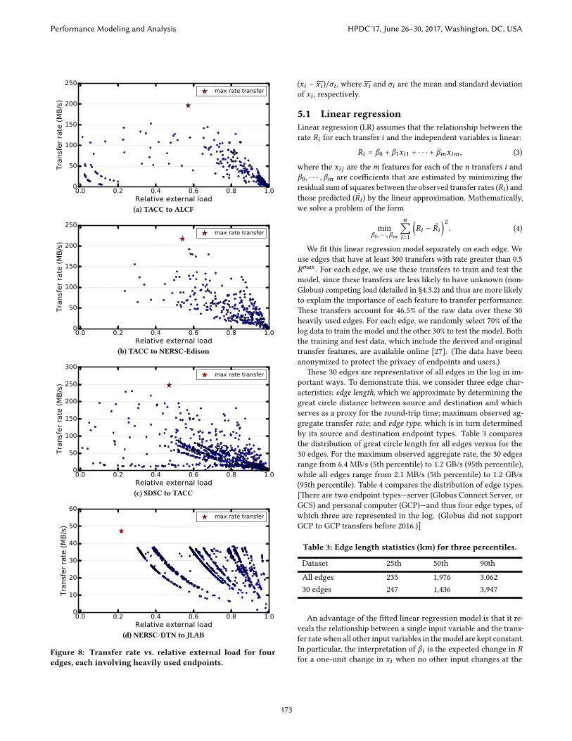
4.3.2 Accounting for other competing load. Figure 3 illustrates asituation in which transfer rate varies fairly cleanly with externalload. We see that the highest transfer rate is always achieved whenrelative external load (K ) is zero, as we expect.

In other se�ings, things are more complicated. For example,Figure 8 plots transfer rate versus relative external load for eachtransfer between four edges involving endpoints with high-speednetworks and storage systems at the Texas Advanced ComputingCenter (TACC), Argonne Leadership Computing Facility (ALCF),National Energy Research Scienti�c Computing Center (NERSC:two di�erent endpoints), San Diego Supercomputer Center (SDSC),and Je�erson Laboratory (JLAB). Here, the relationship betweenknown external load and achieved transfer rate is less clear. Infact, with the exception of the NERSC-DTN to the JLAB edge, themaximum observed transfer rate (marked by a red star) is at a pointother than when the load from other Globus transfers is the lowest.

One likely reason for this discrepancy is competition from non-Globus activities, such as �le transfers performed with other tools,storage activities performed by other tasks, and other tra�c onnetwork link(s) between source and destination. We explore suche�ects in §5.5.2, but in general we have no information that wecan use to quantify this other competing load. �us, we address thelimitation of missing information on non-Globus load by consid-ering in our analyses only transfers that achieve a high fractionof peak, under the hypothesis that these transfers are unlikely tohave su�ered from much other competing load. Speci�cally, foreach edge, E, we �rst determine the highest transfer rate achievedbetween the two endpoints, Rmax (E), and then remove from ourdataset transfers that have a rate less than T.Rmax (E), where T is aload threshold, set to 0.5 except where otherwise speci�ed.

�is approach is not ideal. It may also remove transfers thatperform badly because of, for example, transfer characteristics(e.g., small �les). However, we show in §5.5 that the accuracyof our models improves with load threshold. wide area networkconditions.

5 REGRESSION ANALYSISWe use regression analysis to explain the relationship between thetransfer rate and the 15 independent variables in Table 2. In partic-ular, we investigate whether the transfer rate can be modeled as alinear and nonlinear combination of independent variables. To testlinear dependence, we use linear regression to �t the data. For thenonlinear testing, there exists a wide range of supervised-machine-learning algorithms of varying complexity. We use gradient boost-ing [9], a state-of-the-art supervised-machine-learning algorithmthat has proven e�ective on many predictive modeling tasks.

Both methods bene�t from preprocessing since the scale of theindependent variables is quite di�erent. �erefore, we normalizeeach input xi to have zero mean and unit variance, se�ing x ′ =


172


0

50

100

150

200

250

Tran

sfer

rate

(MB/

s)

max rate transfer

(a) TACC to ALCF


0

50

100

150

200

250

Tran

sfer

rate

(MB/

s)

max rate transfer

(b) TACC to NERSC-Edison


0

50

100

150

200

250

300

Tran

sfer

rate

(MB/

s)

max rate transfer

(c) SDSC to TACC


0

10

20

30

40

50

60

Tran

sfer

rate

(MB/

s)

max rate transfer

(d) NERSC-DTN to JLAB

Figure 8: Transfer rate vs. relative external load for fouredges, each involving heavily used endpoints.

(xi − xi )/σi , where xi and σi are the mean and standard deviationof xi , respectively.

5.1 Linear regressionLinear regression (LR) assumes that the relationship between therate Ri for each transfer i and the independent variables is linear:

Ri = β0 + β1xi1 + · · · + βmxim , (3)

where the xi j are them features for each of the n transfers i andβ0, · · · , βm are coe�cients that are estimated by minimizing theresidual sum of squares between the observed transfer rates (Ri ) andthose predicted (R̂i ) by the linear approximation. Mathematically,we solve a problem of the form

minβ0, · · ·,βm

n∑i=1

(Ri − R̂i

)2. (4)

We �t this linear regression model separately on each edge. Weuse edges that have at least 300 transfers with rate greater than 0.5Rmax . For each edge, we use these transfers to train and test themodel, since these transfers are less likely to have unknown (non-Globus) competing load (detailed in §4.3.2) and thus are more likelyto explain the importance of each feature to transfer performance.�ese transfers account for 46.5% of the raw data over these 30heavily used edges. For each edge, we randomly select 70% of thelog data to train the model and the other 30% to test the model. Boththe training and test data, which include the derived and originaltransfer features, are available online [27]. (�e data have beenanonymized to protect the privacy of endpoints and users.)

�ese 30 edges are representative of all edges in the log in im-portant ways. To demonstrate this, we consider three edge char-acteristics: edge length, which we approximate by determining thegreat circle distance between source and destination and whichserves as a proxy for the round-trip time; maximum observed ag-gregate transfer rate; and edge type, which is in turn determinedby its source and destination endpoint types. Table 3 comparesthe distribution of great circle length for all edges versus for the30 edges. For the maximum observed aggregate rate, the 30 edgesrange from 6.4 MB/s (5th percentile) to 1.2 GB/s (95th percentile),while all edges range from 2.1 MB/s (5th percentile) to 1.2 GB/s(95th percentile). Table 4 compares the distribution of edge types.[�ere are two endpoint types—server (Globus Connect Server, orGCS) and personal computer (GCP)—and thus four edge types, ofwhich three are represented in the log. (Globus did not supportGCP to GCP transfers before 2016.)]

Table 3: Edge length statistics (km) for three percentiles.

Dataset 25th 50th 90thAll edges 235 1,976 3,06230 edges 247 1,436 3,947

An advantage of the ��ed linear regression model is that it re-veals the relationship between a single input variable and the trans-fer rate when all other input variables in themodel are kept constant.In particular, the interpretation of βi is the expected change in Rfor a one-unit change in xi when no other input changes at the


173

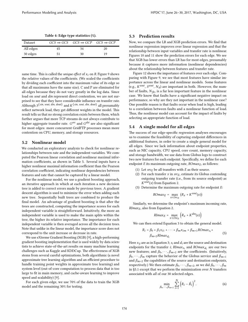
Table 4: Edge type statistics (%).

Dataset GCS ⇒ GCS GCS ⇒ GCP GCS ⇒ GCP

All edges 45 34 2030 edges 51 30 19

same time. �is is called the unique e�ect of xi on R. Figure 9 showsthe relative values of the coe�cients. (We scaled the coe�cientsby dividing each coe�cient into the maximum value of its edge sothat all maximums have the same size). C and P are eliminated forall edges because they do not vary greatly in the log data. Sinceload on sout and din represent direct contention, we are not sur-prised to see that they have considerable in�uence on transfer rate.Although S{sin, sout, din, dout} and K{sin, sout, din, dout} all presumablyre�ect network load, they get di�erent weights in the model. �isresult tells us that no strong correlation exists between them, whichfurther argues that more TCP streams do not always contribute tohigher aggregate transfer rate. Gsrc and Gdst are also signi�cantfor most edges: more concurrent GridFTP processes mean morecontention on CPU, memory, and storage resources.

5.2 Nonlinear modelWe conducted an exploratory analysis to check for nonlinear re-lationships between rate and the independent variables. We com-puted the Pearson linear correlation and nonlinear maximal infor-mation coe�cients, as shown in Table 5. Several inputs have ahigher nonlinear maximal information coe�cient than the Pearsoncorrelation coe�cient, indicating nonlinear dependencies betweenfeatures and rate that cannot be captured by a linear model.

For the nonlinear model, we use a gradient boosting approach,an iterative approach in which at each iteration a new decisiontree is added to correct errors made by previous trees. A gradientdescent algorithm is used to minimize the error when adding eachnew tree. Sequentially built trees are combined to produce the�nal model. An advantage of gradient boosting is that a�er thetrees are constructed, computing the importance scores for eachindependent variable is straightforward. Intuitively, the more anindependent variable is used to make the main splits within thetree, the higher its relative importance. �e importance for eachindependent variable is then averaged across all the decision trees.Note that unlike in the linear model, the importance score does notcorrespond to the unit increase or decrease in rate.

We use eXtreme Gradient Boosting (XGB) [9], a high-performinggradient boosting implementation that is used widely by data scien-tists to achieve state-of-the-art results on many machine learningchallenges such as Kaggle and KDDCup. �e e�ectiveness of XGBstems from several careful optimizations, both algorithmic (a novelapproximate tree learning algorithm and an e�cient procedure tohandle training point weights in approximate tree learning) andsystem level (out-of-core computation to process data that is toolarge to �t in main memory, and cache-aware learning to improvespeed and scalability) [9].

For each given edge, we use 70% of the data to train the XGBmodel and the remaining 30% for testing.

5.3 Prediction resultsNow, we compare the LR and XGB prediction errors. We �nd thatnonlinear regression improves over linear regression and that therelationship between input variables and transfer rate is nonlinear.Figures 10 and 11 show the prediction errors for each edge. We seethat XGB has lower errors than LR has for most edges, presumablybecause it captures more information (nonlinear dependencies)about the relationship between features and transfer rate.

Figure 12 shows the importance of features over each edge. Com-paring with Figure 9, we see that most features have similar im-portance across the linear and nonlinear models. Some features(e.g., Ksout , Ssout , N b) are important in both. However, the num-ber of faults, N�t , is a far less important feature in the nonlinearcase. We know that faults have a signi�cant negative impact onperformance, so why are they not important in the nonlinear case?One possible reason is that faults occur when load is high, leadingto a correlation between faults and a nonlinear function of load.�us, the nonlinear model can account for the impact of faults byselecting an appropriate function of load.

5.4 A single model for all edges�e success of our edge-speci�c regression analyses encouragesus to examine the feasibility of capturing endpoint di�erences inadditional features, in order to create a single general model forall edges. Since we lack information about endpoint properties,such as NIC capacity, CPU speed, core count, memory capacity,and storage bandwidth, we use data from Globus logs to constructtwo new features for each endpoint. Speci�cally, we de�ne for eachendpoint E its maximum outgoing rate, ROmaxE , as follows:

(1) Let srcE be all transfers with E as their source.(2) For each transfer x in srcE , estimate its Globus contending

outgoing transfer rate (i.e., from its source endpoint) asKsout (x) from Equation 2.

(3) Determine the maximum outgoing rate for endpoint E:

ROmaxE = maxx ∈SrcE

(Rx + K sout (x )

)Similarly, we determine the endpoint’s maximum incoming rate,

RImaxE , also from Equation 2.

RImaxE = maxx ∈DstE

(Rx + Kdin(x )

)We can then extend Equation 3 to obtain the general model.

Ri = β0 + β1xi1 + · · · + βmxim + βm+1ROmaxsi +βm+2RImaxdi

(5)

Here xij are as in Equation 3; si and di are the source and destinationendpoints for the transfer i; RImaxsi and ROmaxdi are our twonew features; and β0, · · · , βm+2 are the coe�cients. (Intuitively,β0, · · · , βm capture the behavior of the Globus service and βm+1and βm+2 the capabilities of the source and destination endpoints,respectively.) We then estimate β0, · · · , βm+2, as we did β0, · · · , βmin §5.1 except that we perform the minimization over N transfersassociated with all of our 30 selected edges.

minβ0, · · ·,βm+2

N∑i=1

(Ri − R̂i

)2. (6)


174

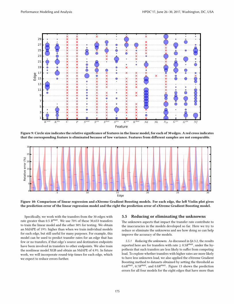
K sout K din C P S sout S sin S dout S din K sin K dout Nd Nb Nflt G src G dst Nf

Feature

13579

11131517192123252729

Edge

Figure 9: Circle size indicates the relative signi�cance of features in the linearmodel, for each of 30 edges. A red cross indicatesthat the corresponding feature is eliminated because of low variance. Features from di�erent samples are not comparable.

5 10 15 20 25 30Edge

0

5

10

15

20

25

30

Rela

tive

erro

r (%

)

Figure 10: Comparison of linear regression and eXtreme Gradient Boosting models. For each edge, the le� Violin plot givesthe prediction error of the linear regression model and the right the prediction error of eXtreme Gradient Boosting model.

Speci�cally, we work with the transfers from the 30 edges withrate greater than 0.5 Rmax . We use 70% of these 30,653 transfersto train the linear model and the other 30% for testing. We obtainan MdAPE of 19%: higher than when we train individual modelsfor each edge, but still useful for many purposes. For example, thismodel can be used to predict transfer rates for an edge that hasfew or no transfers, if that edge’s source and destination endpointshave been involved in transfers to other endpoints. We also trainthe nonlinear model XGB and obtain an MdAPE of 4.9%. In futurework, we will incorporate round-trip times for each edge, whichwe expect to reduce errors further.

5.5 Reducing or eliminating the unknowns�e unknown aspects that impact the transfer rate contribute tothe inaccuracies in the models developed so far. Here we try toreduce or eliminate the unknowns and see how doing so can helpimprove the accuracy of the models.

5.5.1 Reducing the unknowns. As discussed in §4.3.2, the resultsreported here are for transfers with rate ≥ 0.5Rmax , under the hy-pothesis that such transfers are less likely to su�er from competingload. To explore whether transfers with higher rates are more likelyto have less unknown load, we also applied the eXtreme GradientBoosting method to datasets obtained by se�ing the threshold as0.6Rmax , 0.7Rmax , and 0.8Rmax . Figure 13 shows the predictionerrors for all four models for the eight edges that have more than


175

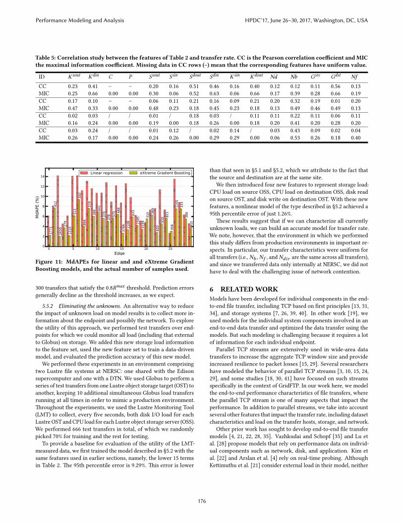
Table 5: Correlation study between the features of Table 2 and transfer rate. CC is the Pearson correlation coe�cient and MICthe maximal information coe�cient. Missing data in CC rows (–) mean that the corresponding features have uniform value.

ID Ksout Kdin C P Ssout Ssin Sdout Sdin Ksin Kdout Nd Nb Gsrc Gdst Nf

CC 0.23 0.41 – – 0.20 0.16 0.51 0.46 0.16 0.40 0.12 0.12 0.11 0.56 0.13MIC 0.25 0.66 0.00 0.00 0.30 0.06 0.52 0.63 0.06 0.66 0.17 0.39 0.28 0.66 0.19CC 0.17 0.10 – – 0.06 0.11 0.21 0.16 0.09 0.21 0.20 0.32 0.19 0.01 0.20MIC 0.47 0.33 0.00 0.00 0.48 0.23 0.18 0.45 0.23 0.18 0.13 0.49 0.46 0.49 0.13CC 0.02 0.03 / / 0.01 / 0.18 0.03 / 0.11 0.11 0.22 0.11 0.06 0.11MIC 0.16 0.24 0.00 0.00 0.19 0.00 0.18 0.26 0.00 0.18 0.20 0.41 0.20 0.28 0.20CC 0.03 0.24 / / 0.01 0.12 / 0.02 0.14 / 0.03 0.43 0.09 0.02 0.04MIC 0.26 0.17 0.00 0.00 0.24 0.26 0.00 0.29 0.29 0.00 0.06 0.53 0.26 0.18 0.40

0 5 10 15 20 25Edge

0

2

4

6

8

10

12

14

MdA

PE (%

)

2771

412

3459

279

1210

513

350

894

574

388 64

137

037

8 570 48

837

66 1108

633

1595

4194

310 36

942

091

9 811

456

1105

333

388

915

Linear regression eXtreme Gradient Boosting

Figure 11: MdAPEs for linear and and eXtreme GradientBoosting models, and the actual number of samples used.

300 transfers that satisfy the 0.8Rmax threshold. Prediction errorsgenerally decline as the threshold increases, as we expect.

5.5.2 Eliminating the unknowns. An alternative way to reducethe impact of unknown load on model results is to collect more in-formation about the endpoint and possibly the network. To explorethe utility of this approach, we performed test transfers over end-points for which we could monitor all load (including that externalto Globus) on storage. We added this new storage load informationto the feature set, used the new feature set to train a data-drivenmodel, and evaluated the prediction accuracy of this new model.

We performed these experiments in an environment comprisingtwo Lustre �le systems at NERSC: one shared with the Edisonsupercomputer and one with a DTN. We used Globus to perform aseries of test transfers from one Lustre object storage target (OST) toanother, keeping 10 additional simultaneous Globus load transfersrunning at all times in order to mimic a production environment.�roughout the experiments, we used the Lustre Monitoring Tool(LMT) to collect, every �ve seconds, both disk I/O load for eachLustre OST andCPU load for each Lustre object storage server (OSS).We performed 666 test transfers in total, of which we randomlypicked 70% for training and the rest for testing.

To provide a baseline for evaluation of the utility of the LMT-measured data, we �rst trained the model described in §5.2 with thesame features used in earlier sections, namely, the lower 15 termsin Table 2. �e 95th percentile error is 9.29%. �is error is lower

than that seen in §5.1 and §5.2, which we a�ribute to the fact thatthe source and destination are at the same site.

We then introduced four new features to represent storage load:CPU load on source OSS, CPU load on destination OSS, disk readon source OST, and disk write on destination OST. With these newfeatures, a nonlinear model of the type described in §5.2 achieved a95th percentile error of just 1.26%.

�ese results suggest that if we can characterize all currentlyunknown loads, we can build an accurate model for transfer rate.We note, however, that the environment in which we performedthis study di�ers from production environments in important re-spects. In particular, our transfer characteristics were uniform forall transfers (i.e., Nb , Nf , and Ndir are the same across all transfers),and since we transferred data only internally at NERSC, we did nothave to deal with the challenging issue of network contention.

6 RELATEDWORKModels have been developed for individual components in the end-to-end �le transfer, including TCP based on �rst principles [13, 31,34], and storage systems [7, 26, 39, 40]. In other work [19], weused models for the individual system components involved in anend-to-end data transfer and optimized the data transfer using themodels. But such modeling is challenging because it requires a lotof information for each individual endpoint.

Parallel TCP streams are extensively used in wide-area datatransfers to increase the aggregate TCP window size and provideincreased resilience to packet losses [15, 29]. Several researchershave modeled the behavior of parallel TCP streams [3, 10, 15, 24,29], and some studies [18, 30, 41] have focused on such streamsspeci�cally in the context of GridFTP. In our work here, we modelthe end-to-end performance characteristics of �le transfers, wherethe parallel TCP stream is one of many aspects that impact theperformance. In addition to parallel streams, we take into accountseveral other features that impact the transfer rate, including datasetcharacteristics and load on the transfer hosts, storage, and network.

Other prior work has sought to develop end-to-end �le transfermodels [4, 21, 22, 28, 35]. Vazhkudai and Schopf [35] and Lu etal. [28] propose models that rely on performance data on individ-ual components such as network, disk, and application. Kim etal. [22] and Arslan et al. [4] rely on real-time probing. AlthoughKe�imuthu et al. [21] consider external load in their model, neither


176

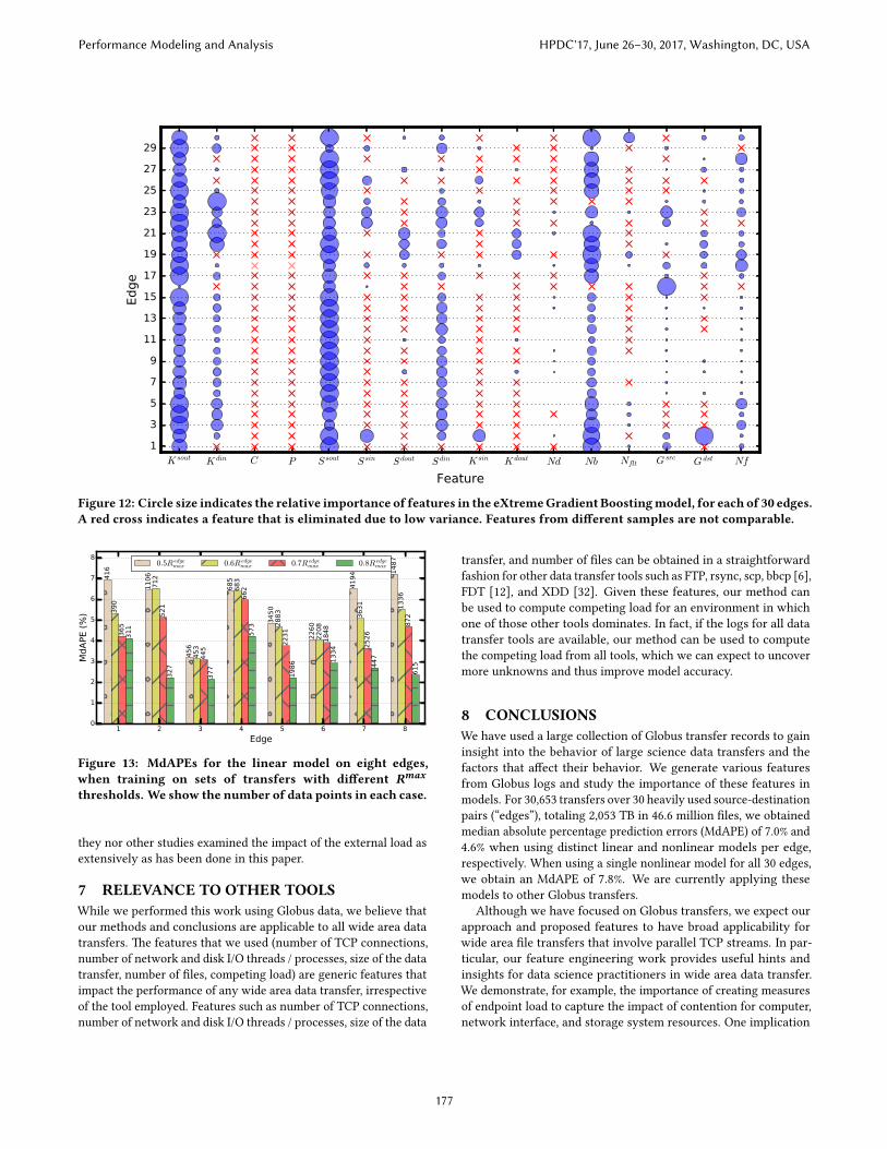
K sout K din C P S sout S sin S dout S din K sin K dout Nd Nb Nflt G src G dst Nf

Feature

13579

11131517192123252729

Edge

Figure 12: Circle size indicates the relative importance of features in the eXtremeGradient Boostingmodel, for each of 30 edges.A red cross indicates a feature that is eliminated due to low variance. Features from di�erent samples are not comparable.

1 2 3 4 5 6 7 8Edge

0

1

2

3

4

5

6

7

8

MdA

PE (%

)

416

390

365

311

1106

712

521

327

456

453

445

377

685

683

662

573 34

5028

8322

3119

86

2260

2208

1848

1334

4194

3631

2526

447

1487

1336

872

615

0:5R edgemax 0:6R edge

max 0:7R edgemax 0:8R edge

max

Figure 13: MdAPEs for the linear model on eight edges,when training on sets of transfers with di�erent Rmax

thresholds. We show the number of data points in each case.

they nor other studies examined the impact of the external load asextensively as has been done in this paper.

7 RELEVANCE TO OTHER TOOLSWhile we performed this work using Globus data, we believe thatour methods and conclusions are applicable to all wide area datatransfers. �e features that we used (number of TCP connections,number of network and disk I/O threads / processes, size of the datatransfer, number of �les, competing load) are generic features thatimpact the performance of any wide area data transfer, irrespectiveof the tool employed. Features such as number of TCP connections,number of network and disk I/O threads / processes, size of the data

transfer, and number of �les can be obtained in a straightforwardfashion for other data transfer tools such as FTP, rsync, scp, bbcp [6],FDT [12], and XDD [32]. Given these features, our method canbe used to compute competing load for an environment in whichone of those other tools dominates. In fact, if the logs for all datatransfer tools are available, our method can be used to computethe competing load from all tools, which we can expect to uncovermore unknowns and thus improve model accuracy.

8 CONCLUSIONSWe have used a large collection of Globus transfer records to gaininsight into the behavior of large science data transfers and thefactors that a�ect their behavior. We generate various featuresfrom Globus logs and study the importance of these features inmodels. For 30,653 transfers over 30 heavily used source-destinationpairs (“edges”), totaling 2,053 TB in 46.6 million �les, we obtainedmedian absolute percentage prediction errors (MdAPE) of 7.0% and4.6% when using distinct linear and nonlinear models per edge,respectively. When using a single nonlinear model for all 30 edges,we obtain an MdAPE of 7.8%. We are currently applying thesemodels to other Globus transfers.

Although we have focused on Globus transfers, we expect ourapproach and proposed features to have broad applicability forwide area �le transfers that involve parallel TCP streams. In par-ticular, our feature engineering work provides useful hints andinsights for data science practitioners in wide area data transfer.We demonstrate, for example, the importance of creating measuresof endpoint load to capture the impact of contention for computer,network interface, and storage system resources. One implication


177

is that contention at endpoints can signi�cantly reduce aggregateperformance of even overprovisioned networks. �is result sug-gests that aggregate performance can be improved by schedulingtransfers and/or reducing concurrency and parallelism.

We have identi�ed several directions for improved transfer ser-vice monitoring that we hope can improve our models by improvingknowledge of other loads. Globus currently records informationonly about its transfers: it collects no information about non-Globusload on endpoints or about network load. A new version with theability to monitor overall endpoint status is under development.Further research is needed to study the in�uence of network load.To this end, we plan to incorporate SNMP data from routers to char-acterize network conditions. Another direction for future work is tosee whether more advanced machine learning methods, for exam-ple multiobjective modeling with machine learning (AutoMOMML)[5], can yield be�er models.

ACKNOWLEDGMENTS�is material was supported in part by the U.S. Department ofEnergy, O�ce of Science, Advanced Scienti�c Computing Research,under Contract DE-AC02-06CH11357. We thank Nagi Rao for usefuldiscussions, Brigi�e Raumann for help with Globus log analysis,Glenn Lockwood for help with experiments at NERSC described in§5.5, and the Globus team for much good work and advice.

REFERENCES[1] W. Allcock, J. Bresnahan, R. Ke�imuthu, M. Link, C. Dumitrescu, I. Raicu, and

I. Foster. �e Globus striped GridFTP framework and server. In SC’05, pages54–61, 2005.

[2] B. Allen, J. Bresnahan, L. Childers, I. Foster, G. Kandaswamy, R. Ke�imuthu,J. Kordas, M. Link, S. Martin, K. Picke�, and S. Tuecke. So�ware as a service fordata scientists. Commun. ACM, 55(2):81–88, Feb. 2012.

[3] E. Altman, D. Barman, B. Tu�n, and M. Vojnovic. Parallel TCP sockets: Sim-ple model, throughput and validation. In 25th IEEE Intl Conf. on ComputerCommunications, pages 1–12, April 2006.

[4] E. Arslan, K. Guner, and T. Kosar. HARP: predictive transfer optimization basedon historical analysis and real-time probing. In SC’16, pages 25:1–25:12, 2016.

[5] P. Balaprakash, A. Tiwari, S. M. Wild, and P. D. Hovland. AutoMOMML: Auto-matic Multi-objective Modeling with Machine Learning. In ISC, pages 219–239,2016.

[6] BBCP. h�p://www.slac.stanford.edu/∼abh/bbcp/.[7] P. H. Carns, B. W. Se�lemyer, and W. B. Ligon III. Using server-to-server commu-

nication in parallel �le systems to simplify consistency and improve performance.In SC’08, page 6, 2008.

[8] K. Chard, S. Tuecke, and I. Foster. Globus: Recent enhancements and futureplans. In XSEDE’16, page 27. ACM, 2016.

[9] T. Chen and C. Guestrin. XGBoost: A scalable tree boosting system. arXivpreprint arXiv:1603.02754, 2016.

[10] J. Crowcro� and P. Oechslin. Di�erentiated end-to-end internet services usinga weighted proportional fair sharing TCP. SIGCOMM Comput. Commun. Rev.,28(3):53–69, July 1998.

[11] E. Dart, L. Rotman, B. Tierney, M. Hester, and J. Zurawski. �e Science DMZ:A network design pa�ern for data-intensive science. Scienti�c Programming,22(2):173–185, 2014.

[12] FDT. FDT - Fast Data Transfer. h�p://monalisa.cern.ch/FDT/.[13] J. Gao and N. S. V. Rao. TCP AIMD dynamics over Internet connections. IEEE

Communications Le�ers, 9:4–6, 2005.[14] I. Guyon and A. Elissee�. An introduction to variable and feature selection. J.

Mach. Learn. Res., 3:1157–1182, Mar. 2003.[15] T. J. Hacker, B. D. Athey, and B. Noble. �e end-to-end performance e�ects

of parallel TCP sockets on a lossy wide-area network. In 16th Intl Parallel andDistributed Processing Symp., page 314, 2002.

[16] A. Hanemann, J. W. Boote, E. L. Boyd, J. Durand, L. Kudarimoti, R. Lapacz, D. M.Swany, S. Trocha, and J. Zurawski. PerfSONAR: A service oriented architecturefor multi-domain network monitoring. In 3rd Intl Conf. on Service-OrientedComputing, pages 241–254, Berlin, Heidelberg, 2005. Springer-Verlag.

[17] iperf3. h�p://so�ware.es.net/iperf/.

[18] T. Ito, H. Ohsaki, and M. Imase. GridFTP-APT: Automatic parallelism tuningmechanism for data transfer protocol GridFTP. In 6th IEEE Intl Symp. on ClusterComputing and the Grid, pages 454–461, 2006.

[19] E.-S. Jung, R. Ke�imuthu, and V. Vishwanath. Toward optimizing disk-to-disktransfer on 100G networks. In 7th IEEE Intl Conf. on Advanced Networks andTelecommunications Systems, 2013.

[20] T. Kelly. Scalable TCP: Improving performance in highspeed wide area networks.ACM SIGCOMM Computer Communication Review, 33(2):83–91, 2003.

[21] R. Ke�imuthu, G. Vardoyan, G. Agrawal, and P. Sadayappan. Modeling andoptimizing large-scale wide-area data transfers. 14th IEEE/ACM Intl Symp. onCluster, Cloud and Grid Computing, 0:196–205, 2014.

[22] J. Kim, E. Yildirim, and T. Kosar. A highly-accurate and low-overhead predictionmodel for transfer throughput optimization. Cluster Computing, 18(1):41–59,2015.

[23] E. Kissel, M. Swany, B. Tierney, and E. Pouyoul. E�cient wide area data transferprotocols for 100 Gbps networks and beyond. In 3rd Intl Workshop on Network-Aware Data Management, page 3. ACM, 2013.

[24] G. Kola and M. K. Vernon. Target bandwidth sharing using endhost measures.Perform. Eval., 64(9-12):948–964, Oct. 2007.

[25] T. Kosar, G. Kola, and M. Livny. Data pipelines: Enabling large scale multi-protocol data transfers. In 2nd Workshop on Middleware for Grid Computing,pages 63–68, 2004.

[26] N. Liu, C. Carothers, J. Cope, P. Carns, R. Ross, A. Crume, and C. Maltzahn.Modeling a leadership-scale storage system. In Parallel Processing and AppliedMathematics, pages 10–19. 2012.

[27] Z. Liu, P. Balaprakash, R. Ke�imuthu, and I. Foster. Explaining wide area datatransfer performance. h�p://hdl.handle.net/11466/globus A4N55BB, 2017.

[28] D. Lu, Y. Qiao, P. Dinda, and F. Bustamante. Characterizing and predicting TCPthroughput on the wide area network. In 25th IEEE Intl Conf. on DistributedComputing Systems, pages 414–424, June 2005.

[29] D. Lu, Y. Qiao, P. A. Dinda, and F. E. Bustamante. Modeling and taming parallelTCP on the wide area network. In 19th IEEE Intl Parallel and Distributed ProcessingSymp., page 68b, 2005.

[30] H. Ohsaki and M. Imase. On modeling GridFTP using �uid-�ow approximationfor high speed Grid networking. In Symp. on Applications and the Internet–Workshops, pages 638–, 2004.

[31] J. Padhye, V. Firoiu, D. F. Towsley, and J. F. Kurose. Modeling TCP Reno perfor-mance: A simple model and its empirical validation. IEEE/ACMTrans. Networking,8(2):133–145, 2000.

[32] B. W. Se�lemyer, J. D. Dobson, S. W. Hodson, J. A. Kuehn, S. W. Poole, and T. M.Ruwart. A technique for moving large data sets over high-performance longdistance networks. In 27th Symp. on Mass Storage Systems and Technologies,pages 1–6, May 2011.

[33] B. Tierney, W. Johnston, B. Crowley, G. Hoo, C. Brooks, and D. Gunter. �eNetLogger methodology for high performance distributed systems performanceanalysis. In 7th Intl Symp. on High Performance Distributed Computing, pages260–267, 1998.

[34] G. Vardoyan, N. S. V. Rao, and D. Towsley. Models of TCP in high-BDP environ-ments and their experimental validation. In 24th Intl Conf. on Network Protocols,pages 1–10, 2016.

[35] S. Vazhkudai and J. Schopf. Using regression techniques to predict large datatransfers. Int. J. High Perf. Comp. Appl., 2003.

[36] D. X. Wei, C. Jin, S. H. Low, and S. Hegde. FAST TCP: Motivation, architecture,algorithms, performance. IEEE/ACM Trans. Networking, 14(6):1246–1259, 2006.

[37] W. Weibull. A statistical distribution function of wide applicability. Journal ofApplied Mechanics, pages 293–297, 1951.

[38] R. Wolski. Forecasting network performance to support dynamic schedulingusing the Network Weather Service. In 6th IEEE Symp. on High PerformanceDistributed Computing, 1997.

[39] J. M. Wozniak, S. W. Son, and R. Ross. Distributed object storage rebuild analysisvia simulation with GOBS. In Intl Conf. on Dependable Systems and NetworksWorkshops, pages 23–28, 2010.

[40] Q. M. Wu, K. Xie, M. F. Zhu, L. M. Xiao, and L. Ruan. DMFSsim: A distributedmetadata �le system simulator. Applied Mechanics and Materials, 241:1556–1561,2013.

[41] E. Yildirim, D. Yin, and T. Kosar. Prediction of optimal parallelism level in widearea data transfers. IEEE Trans. Parallel Distrib. Syst., 22(12):2033–2045, Dec.2011.


178

http://www.slac.stanford.edu/~abh/bbcp/

http://monalisa.cern.ch/FDT/

http://software.es.net/iperf/

http://hdl.handle.net/11466/globus_A4N55BB

Documents

Explaining Wide Area Data Transfer Performancekettimut/publications/hpdc17-final.pdfExplaining Wide Area Data Transfer Performance Zhengchun Liu Argonne National Laboratory Lemont,