Expert Systems with Applications 39 (2012) 10226–10235

Contents lists available at SciVerse ScienceDirect

Expert Systems with Applications

journal homepage: www.elsevier .com/locate /eswa

On-line adaptive clustering for process monitoring and fault detection

Milena Petkovic a, Milan R. Rapaic a,⇑, Zoran D. Jelicic a, Alessandro Pisano b

a Faculty of Technical Sciences, University of Novi Sad, Serbiab Department of Electrical and Electronic Engineering, University of Cagliari, Cagliari, Italy

a r t i c l e i n f o

Keywords:Fault detection and isolationReal-time expert systemsAdaptive clusteringAdaptive diagnosisNovelty detection

0957-4174/$ - see front matter � 2012 Elsevier Ltd. Adoi:10.1016/j.eswa.2012.02.150

⇑ Corresponding author.E-mail addresses: milena5@uns.ac.rs (M.

(M.R. Rapaic), jelicic@uns.ac.rs (Z.D. Jelicic), pisano@u

a b s t r a c t

An adaptive clustering procedure specifically designed for process monitoring, fault detection and isola-tion is presented in this paper. The key feature of the proposed procedure can be identified as its under-lying capability to detect novelties in the system’s mode of operation and, thus, to identify previouslyunseen functioning modes of the process. Once a novelty is detected, relevant informations are used toenrich the knowledge-base of the algorithm and as a result the proposed clustering procedure evolvesand learns the new features of the monitored process in accordance with the available process data.The suggested clustering procedure is theoretically illustrated and its effectiveness has been investigatedexperimentally. Particularly, the on-line implementation of the algorithm and its integration with a faultdetection expert system have been considered by making reference to a pneumatic process.

� 2012 Elsevier Ltd. All rights reserved.

1. Introduction

Fault detection and isolation (FDI) is an important field in mod-ern process engineering. A fault can be defined as a deviation froman acceptable range of an observed variable or a calculated param-eter associated with the process (Venkatasubramanian et al.,2003a). More generally, a fault can be seen as a deviation froman acceptable working condition. A related notion of failure or mal-functioning is an underlying event causing the abnormality in pro-cess operation. Clearly, early detection of abnormal events and ofunwanted/unexpected working conditions is crucial for timelytriggering the appropriate corrective actions that prevents furtherpropagation of the abnormal behaviour thus reducing productivityloss and/or recovering safety in the system’s operation.

In recent decades much effort has been spent in the area of fail-ure diagnosis, both in academia and among practitioners. An intro-duction to the basic principles of industrial safety, reliability andhazard analysis can be found in Love (2007). For an overview ofvarious fault detection techniques we refer to Iserman (2006), Ding(2008), Venkatasubramanian et al. (2003a, 2003b, 2003c). Faultdiagnosis techniques can roughly be classified as either model-based or process history-based methods. In Venkatasubramanianet al. (2003a) a general framework has been proposed in whichany fault diagnostic decision-making process can be seen as a ser-ies of transformations acting on measured process variables. Insuch a framework, measurements are first used to calculateprocess features. Feature calculation is problem specific and, in

ll rights reserved.

Petkovic), rapaja@uns.ac.rsnica.diee.it (A. Pisano).

general, requires certain amount of a priori process knowledge.By means of a classification procedure, features are used to identifycurrent process working condition as either nominal or faulty. Asophisticated fault classifier could be capable of distinguishingamong a number of faulty conditions, thus performing fault isola-tion. Whatever the case may be, apart from feature extraction, clas-sification is a crucial part of any fault diagnosis scheme.

A number of classification and clustering algorithms have beenfruitfully applied in different areas of engineering. A general surveyof statistical approaches can be found in Izenman (2008), while anintroduction to a broader field of statistical decision theory can befound in Berger (2006). Various soft-computing techniques forclassification, including neural networks, fuzzy logic and supportvector machines, are presented in Kecman (2001). In-depth analy-sis of various kernel-based classifiers can be found in Schölkopfand Smola (2002). A number of different decision making systemsfor process monitoring and fault detection have been proposed re-cently. A survey of qualitative approaches is presented in Venkat-asubramanian et al. (2003b), and some other examples can befound in White and Lakany (2008), Mendonca et al. (2009), Tangand Wang (2008), Quian et al. (2003), Matic et al. (2012), andKanovic et al. (in press).

Most of the existing fault diagnosis techniques assume the apriori characterization of all possible operating conditions, someof which labelled as nominal and some as faulty. In some cases,however, it is rather hard to predict all possible failures in advance.This is especially true in process industry where plants operate in adynamic environment and under the influence of numerous uncer-tainty factors. Therefore, it would be preferable to devise diagnos-tic schemes capable of learning from the process data stream byidentifying the different modes of operations automatically.

M. Petkovic et al. / Expert Systems with Applications 39 (2012) 10226–10235 10227

However, this is not an easy task and the problem of on-line nov-elty detection still remains an open issue (see e.g. Markou andSingh, 2003a, 2003b).

1.1. Contribution and structure of the paper

The main aim of this paper is to propose an approach endowedby capabilities of on-line novelties detection, where the noveltiesin question correspond to changes in the mode of operation of adynamic process. The proposed procedure can be seen as an evolv-ing classification technique and is inspired by the on-line identifi-cation procedure presented in Angelov and Filev (2004) and moregenerally by the eClass family of evolving fuzzy classifiers (Angelovet al., 2010).

We introduce appropriate modifications to the methodologypresented in Angelov and Filev (2004) that improve the achievedperformance, in the context of data driven process FDI, and makethe approach easier to implement on-line. In particular, we gener-alize the notion of information potential, which is of crucial impor-tance both for the methodology presented in the present work andfor the developments presented in Angelov and Filev (2004). First,by introducing the forgetting factor into the definition of the infor-mation potential, the sensitivity of the proposed procedure to nov-elties is greatly enhanced (see Example 1). Also, by introducing theforgetting factor, the recursive formulas for evaluation of the infor-mation potential become time-invariant, which is particularly suit-able for on-line implementation. Further, the flexibility of theapproach is enhanced by utilization of weighted norms when com-puting the information potential.

The outline of the paper is as follows. The fundamental notionof information potential is introduced in Section 2. The adaptiveclustering procedure suggested in the present paper is describedin Section 3. The experimental verification of the suggested meth-odology is presented in Section 4 by making reference to a simplepneumatic laboratory-size process. Concluding remarks are givenin Section 5 where an overall evaluation of the proposed procedureis also presented together with potential generalizations and com-binations with alternative approaches to FDI.

2. Information potential

The notion of the information potential has been used in connec-tion with the eClass family of evolving fuzzy classification algo-rithms (Angelov and Filev, 2004; Angelov et al., 2010). Aredefinition of this notion in a way that is more suitable for its con-crete application in process FDI is outlined below, which is one ofthe central contributions of the present work.

Let zi 2 Rn denote a feature vector extracted from the processdata at the discrete time instant i 2 {0,1,2, . . .}, and let

Zk ¼ ðz0; z1; . . . ; zkÞ 2 Rnkþ1 ¼

defRn � Rn � � � � � Rn|fflfflfflfflfflfflfflfflfflfflfflfflfflfflfflffl{zfflfflfflfflfflfflfflfflfflfflfflfflfflfflfflffl}

kþ1times

ð1Þ

denote the ordered set of all process features obtained up to thek-th discrete time instant. Let z 2 Rn be an arbitrary point withinthe feature space. The average square distance of z with respectto the set Zk, as defined in Angelov and Filev (2004), and Angelovet al. (2010), takes the form

Sðz;ZkÞ ¼1

kþ 1

Xk

i¼0

kz� zkk22: ð2Þ

where kqk22 ¼ qT q is the standard squared Euclidean norm of a gen-

eric column vector q 2 Rn. The average square distance can beunderstood as a measure of the ‘‘discrepancy’’ between the pointz and the set Zk of currently available feature vectors.

The information potential, as defined in Angelov and Filev(2004), is a related similarity measure having the form

Pðz;ZkÞ ¼1

1þ Sðz;ZkÞ: ð3Þ

Since the average square distance Sðz;ZkÞ is always a nonnegativenumber whatever the feature point z and the set Zk are given by,it yields that the information potential will always belong to therange

Pðz;ZkÞ 2 ð0;1� 8z 2 Rn; 8Zk 2 Rnk : ð4Þ

If the information potential of a certain point z in the feature spaceis close to the unit value then the corresponding average square dis-tance is small, which means that z is a good representative of thefeature points belonging to the set Zk. If, on the contrary, the infor-mation potential is close to zero then the corresponding averagesquare distance is large and the feature point z is not well repre-sented by the elements of Zk.

When applied to process fault detection problems, however, theabove notions and measures give rise to some drawbacks. In fact,the entire process history is taken into consideration in the defini-tions (2) and (3). In the real processes operation, however, it is of-ten the nature of faults to occur after long periods of healthybehaviour.

As a result, immediately after the occurrence of a fault the num-ber of feature vectors in the set Zk denoting faulty behaviour willbe, typically, significantly smaller than the corresponding numberof features associated to the nominal behaviour. The feature vec-tors acquired after the occurrence of the fault will have a largeaverage square distance and, consequently, small value of theinformation potential that will slowly increase as time goes on.As shown by means of the simple Example 1, reported below, whenthe fault occurs after a long time interval of healthy operation itcan arise a long delay before that an information potential basedalgorithm can recognize the faulty status as the actual operatingmode of the process.

We suggest in this paper to use different similarity measures inorder to attenuate the drawbacks previously mentioned therebymaking the fault detection algorithm more sensitive to noveltiesand capable of more promptly detect the occurrence of (possiblydifferent types of) faults.

One of the main ideas introduced in the present paper is to givemore relevance to recent process history when defining the infor-mation potential, and this is done by means of a certain forgettingfactor term.

We then introduce the next weighted average square distancewith forgetting factor k of a feature vector z with respect to thehistorical feature set Zk according to the next definition

Skðz;ZkÞ ¼ ð1� kÞXk

i¼0

kk�ikz� zik2W; ð5Þ

where k 2 (0,1) is the forgetting factor and kqk2W ¼ qT Wq stands for

the squared weighted Euclidean norm, where the scaling matrix Wis supposed to be a symmetric and positive definite matrix ofdimension n. The weighting matrix effectively defines scaling androtation of the feature vectors prior to distance calculations, therebyenhancing the versatility of the given non isotropic measure in thefeature space.

The forgetting factor effectively reduces the size of the processhistory taken into consideration by assigning more relevance to therecent process features as compared to the older ones. Factor(1 � k) in front of (5) is used for normalization purposes only.

The corresponding weighted information potential with for-getting factor is defined, in analogy with (3), as

10228 M. Petkovic et al. / Expert Systems with Applications 39 (2012) 10226–10235

Pkðz;ZkÞ ¼1

1þ Skðz;ZkÞ: ð6Þ

The advantages of using the modified information potential (6),as compared to the previous definition (3), are illustrated by meansof the following academic example

Example 1. Consider a fictitious process with a scalar featurespace z 2 R. Let the zero value of the feature signal z = zn = 0correspond to the nominal process behaviour, whereas the unitvalue z = zf = 1 denotes the occurrence of a fault. Let the process beevolving in the nominal condition during an initial transient andlet the faulty condition occurs starting from the k0-th sample, i.e.

zk ¼0 0 6 k < k0

1 k P k0

�ð7Þ

The faulty condition is detected once the information potential ofthe faulty feature point zf with respect to the historical feature setZk will exceed the information potential of the nominal featurepoint zn (or, equivalently, once the corresponding average squaredistance will becomes smaller). It is the aim of the present exampleto analyse the performance of the fault detection methodology, de-scribed above, in the two cases when the conventional and novelformulations of the information potential are used.

Let the average square distance be defined in accordance withthe expression (2), i.e. without forgetting factor. At any sampletime k P k0 successive to the fault we get

Sðzn;ZkÞ ¼ Sð0;ZkÞ ¼k� k0 þ 1

kþ 1;

Sðzf ;ZkÞ ¼ Sð1;ZkÞ ¼k0

kþ 1:

The fault is detected at the sampling instant k = kd such that

Sðzf ;Zkd Þ < Sðzn;Zkd Þ ) kd ¼ 2k0 þ 1

The detection time kd obtained above depends on the time instantwhen the fault activates, and, particularly, the detection delaykd � k0 (i.e., the number of samples along which the already oc-curred fault goes undetected) is given by k0 + 1, hence it increaseswith the time k0 of fault occurrence, which is highly unsatisfactory.It would be desirable to develop a fault detection algorithm with adetection delay independent of the actual time of fault occurrenceand we are going to show that this is the case using the novel def-inition of information potential and weighted distance.

If, in fact, the relation (5) (with W = 1) is used instead of (2), thenext expressions for the average square distances of the nominaland faulty feature points is obtained for k > k0:

Skðzn;ZkÞ ¼ Skð0;ZkÞ ¼ 1� kk�k0þ1;

Skðzf ;ZkÞ ¼ Skð1;ZkÞ ¼ kk�k0þ1ð1� kk0 Þ:

The fault is detected at time kd such that

Skðzf ;Zkd Þ < Skðzn;Zkd Þ ) kd> k0 � 1þ logk

1þ kkdþ1

2:

The detection delay kd � k0 is now bounded. In fact, one easily getsthe next asymptotics

kd � k0 � �1þ logkð0:5Þ

and thus, except for a short initial transient, the detection delay isindependent of the time when the fault occurs, as desired, showingthe better properties of the suggested modified versions of informa-tion potential and average square distances. h

The weighted average square distance (5), and consequently theweighted information potential (6), will be of practical interest for

real time process monitoring only if a recursive formulation can befound to efficiently address their on-line computation. The nextTheorem 1 is devoted to address this problem by illustrating, andsubstantiating, a recursive algorithm for the on-line computationof the above measures in the general case when the feature vectorz used as first argument of (5) and (6) evolves with time and is cor-respondingly denoted as zk.

Theorem 1. Let Sk ¼ Skðzk;ZkÞ be the weighted average squaredistance of the time varying feature vector zk at the sampling time k(k = 0,1,2, . . .) with respect to the ordered historical feature set Zk.Then, the following recursion holds true for any k P 1:

Sk ¼ kSk�1 þ 2kð1� kÞðzk � zk�1ÞT WFk

þ kð1� kÞkzk � zk�1k2WZk; ð8Þ

Fk ¼ kFk�1 þ kZk�1ðzk�1 � zk�2Þ; ð9ÞZk ¼ kZk�1 þ 1; ð10Þ

where Fk 2 Rn; Zk 2 R, and the initialization values are

S0 ¼ 0; F0 ¼ 0; Z0 ¼ 0: ð11Þ

Proof. Let us note that, for any zk; zi 2 Rn, the next relation can bederived by exploiting standard properties of quadratic forms:

kzk � zik2W ¼ ðzk � ziÞT Wðzk � ziÞ¼ ðzk � zk�1 þ zk�1 � ziÞT Wðzk � zk�1 þ zk�1 � ziÞ¼ ðzk � zk�1ÞT Wðzk � zk�1Þ þ 2ðzk � zk�1ÞT Wðzk�1 � ziÞþ ðzk�1 � ziÞT Wðzk�1 � ziÞ ¼ kzk � zk�1k2

W

þ 2ðzk � zk�1ÞT Wðzk�1 � ziÞ þ kzk�1 � zik2W: ð12Þ

By relying on the above relation (12), the weighted information po-tential of the current feature point can be manipulated as

Sk ¼ð1�kÞXk

i¼0

kk�ikzk�zik2W ¼ð1�kÞ

Xk�1

i¼0

kk�ikzk�zik2W

¼ð1�kÞXk�1

i¼0

kk�ikzk�zk�1k2Wþ2ð1�kÞ

Xk�1

i¼0

kk�iðzk�zk�1ÞT Wðzk�1�ziÞ

þð1�kÞXk�1

i¼0

kk�ikzk�1�zik2W: ð13Þ

Define

Zk ¼Xk�1

i¼0

kk�i: ð14Þ

Then, the first term in the right hand side of (13) can be manipu-lated as follows

ð1� kÞXk�1

i¼0

kk�ikzk � zk�1jj2W ¼ ð1� kÞZkkzk � zk�1k2W ð15Þ

By introducing the quantity

Fk ¼Xk�1

i¼0

kk�iðzk�1 � ziÞ ¼Xk�2

i¼0

kk�iðzk�1 � ziÞ; ð16Þ

the second term in the right hand side of (13) can be manipulated as

2ð1� kÞXk�1

i¼0

kk�iðzk � zk�1ÞT Wðzk�1 � ziÞ

¼ 2ð1� kÞðzk � zk�1ÞT WFk ð17Þ

The last term in the right hand side of (13) can be easily rewrit-ten as follows by taking into account the definition (5)

M. Petkovic et al. / Expert Systems with Applications 39 (2012) 10226–10235 10229

ð1� kÞXk�1

i¼0

kk�ikzk�1 � zik2W ¼ kSk�1: ð18Þ

The recursive expression (8) is thus easily derived by incorporating(14), (16) and (18) into (13). It should also be noted that vector Fk

can be manipulated so as to obtain the next recursion

Fk ¼Xk�2

i¼0

kk�iðzk�1 � zk�2 þ zk�2 � ziÞ

¼Xk�2

i¼0

kk�iðzk�1 � zk�2Þ þXk�2

i¼0

kk�iðzk�2 � ziÞ

¼ kZk�1ðzk�1 � zk�2Þ þ kFk�1: ð19Þthat yields the relation (9) directly. Finally, the recursive formula(10) is straightforwardly obtained from the definition (14). Theorem1 is proven. h

Remark 1. The temporal evolution of the scalar quantity Zk, gov-erned by (14), is clearly independent of the values of the processedfeature vectors. By exploiting well known properties of the geo-metric series it would be straightforward to replace the recursiveformulation (10) by means of the next direct computation formula

Zk ¼1� kk

1� kð20Þ

It is, however, undesirable that the overall recursion dependsexplicitly on the discrete time variable k which is why the aboverelation (20) is not used. Nevertheless, by noticing that the se-quence (20) rapidly converges, for increasing k, towards the con-stant value 1

1�k it could be sought a simplified, approximate,implementation of the overall recursion (8)–(10) by assigning Zk

the constant limit value 11�k.

The next Theorem 2 present a useful recursion for the efficientcalculation of the weighted average square distance (5) in the par-ticular case when the feature vector z used as first argument is fixed,but the historical data set is updated. In the framework of the clus-tering algorithm illustrated in the present paper, indeed, such mea-sure has to be computed, both, for time-varying and fixed featurevectors which is why the next result is useful for our purposes.

Theorem 2. Let z be an arbitrary fixed feature vector and let Zk bethe time varying historical feature set (1). Then, the next recursionholds true at every k P 1

Skðz;ZkÞ ¼ kSkðz;Zk�1Þ þ ð1� kÞkz� zkk2W: ð21Þ

where the initialization value is Sðz;Z0Þ ¼ kz� z0k2W.

Proof. By simple manipulation of (5), the next chain of relation-ships can be written, which proves the Theorem.

Skðz;ZkÞ ¼ ð1� kÞXk

i¼0

kk�ikz� zik2W

¼ ð1� kÞXk�1

i¼0

kk�ikz� zik2W þ ð1� kÞkz� zkk2

W

¼ kSkðz;Zk�1Þ þ ð1� kÞkz� zkk2W: � ð22Þ

Remark 2. The above Theorem 2, particularly relation (21), illus-trates the meaning of the forgetting factor k and its role in the timeevolution of the underlying weighted measure Skðz;ZkÞ. It particu-lar, it shows that Skðz;ZkÞ can be understood as the output signal ofa discrete low pass filter fed by the weighted square distance of zfrom the most recently obtained process feature zk. The pole of theunderlying discrete filter is located at k.

3. An adaptive clustering procedure for on-line classification

The procedure presented in the sequel is inspired by the algo-rithm originally presented in Angelov and Filev (2004). One signif-icant difference is that the information potential is calculated using(5) instead of (2). As shown in the previously given Example 1, thisallows to speed up the detection of the novelties.

The structure and functioning principle of the suggested proce-dure is explained step-wise in the following.

3.1. Feature generation

The first step is to choose a proper generator for the underlyingfeature vectors zk. The features should be descriptive enough to en-able distinction among various operating conditions of the processunder consideration and to allow representing each possible oper-ating condition by a distinct region in the feature space. Kalman fil-ters are widely adopted for on-line feature generation, which willbe our choice, too.

3.2. Initializing the knowledge base

A number of typical operating conditions (including, both, nom-inal and faulty situations) is sometimes known a priori, on the basisof engineering knowledge of the process under consideration. LetMn be the number of a priori known nominal conditions, and letMf the corresponding number of a priori known faulty conditions.Let also M = Mn + Mf denote the overall number of a priori knownoperating conditions.

For each of the a priori known plant working conditions theassociated region in the feature space is identified, and its barycen-ter is selected as a characteristic point of the region. All thesepoints will be denoted as focal points (or simply foci), and willbe referred to as z�i ði ¼ 1;2; . . . ;M). The set of all focal points con-stitutes the initial knowledge-base of the algorithm.

3.3. Classification with static knowledge base

Every sampling instant the weighted information potentialP z�i ;Zk

� �of each focal point is calculated on the basis of the cur-

rently available historical feature set (1). The focus having thehighest information potential value is denoted as the active focusand is considered to be the most descriptive with respect to the re-cent process history.

As a result, the working condition associated to the active focusis designated as the current working condition of the process, i.e.

OpMode ¼ ActFocus ¼ argmaxi

P z�i ;Zk� �

ð23Þ

The important peculiarity of the information potential is that theclassification is made on the basis of the recent process history,rather than just on the current feature vector which may be cor-rupted by noise or in other ways inadequate. The aggregate infor-mation represented by the information potential ensures a certainlevel of robustness of the classification algorithm.

The main drawback of such ‘‘static’’ methodology (in the sensethat the knowledge base is fixed a priori, and no rules and strate-gies for its adaptation have been given yet) is that, in practice,the a priori understanding of the process behaviour is usually lim-ited and incomplete.

It is possible that, for some of the of the a priori known workingconditions, the associated region of the feature space is not se-lected properly, or it has drifted over time for some reasons. Insuch a case the previously selected focus is no longer the mostrepresentative point for the underlying working condition. It is alsopossible that the process under consideration exhibits a

10230 M. Petkovic et al. / Expert Systems with Applications 39 (2012) 10226–10235

completely different behaviour that was not a priori foreseen. Theabove considerations point out that a fixed knowledge base thatdoes not change over time may be not the best choice, whileappropriate methods for the modification or enhancement of theknowledge base (i.e., in other words, a ‘‘learning’’ capability ofthe classification system) would make the algorithm more reliableand robust.

3.4. Continuous adaptation of the knowledge base

To enable the run-time adaptation of the knowledge base, theinformation potential Pðzk;ZkÞ of the newly available feature vec-tor zk is calculated at every sampling instant in parallel to the infor-mation potentials P z�i ;Zk

� �of the focal points. In the previous

Theorems 1 and 2 suitable procedures for the recursive computa-tions of the information potential in the two distinct case of con-stant or time varying feature vector were given.

Most of the time, due to slight process variations, the informa-tion potential of the current feature vector is smaller than theinformation potential of the active foci. When the informationpotential of the newly available feature becomes higher than theinformation potential of all existing foci, the newly available fea-ture is more descriptive with respect to the current process opera-tion than any of the existing focal points and the knowledge-baseof the algorithm should be correspondingly adapted.

In Angelov and Filev (2004) the authors suggested the next con-dition to enable the modification of the knowledge-base

Pðzk;ZkÞ > maxi

P z�i ;Zk

� �: ð24Þ

Here we make use of the modified notion of weighted informationpotential (6), and, furthermore, we suggest a tightened version ofcondition (24), specified as follows

Pkðzk;ZkÞ > maxi

Pk z�i ;Zk

� �þ Pth: ð25Þ

It is worth to remark that condition (25) can be replaced by the nextequivalent one

P�1k ðzk;ZkÞ < min

iP�1

k z�i ;Zk

� �� Pth;1: ð26Þ

which reduces the number of operations to perform at each sam-pling instant since P�1

k ðzk;ZkÞ ¼ 1þ Skðzk;ZkÞ is computed first.The tuning parameters Pth (or, equivalently, Pth,1) are empiricallyselected positive thresholds. It has been found that using (25) or(26) instead of (24) improves the robustness of the algorithm whenthe process measurements are severely corrupted by noise.

Two different decisions can be made upon the positive verifica-tion of condition (25) or (26):

� Replace an existing focal point with the newly available fea-ture vector zk.� Add a new focal point coinciding with the newly available fea-

ture vector zk.

The decision of replacing an existing focal point is taken, obvi-ously, when the newly available feature is close to some of theexisting focal points. The closeness is measured in terms of theweighted Euclidean norm k � kW. Thus when the next conditionholds

mini

zk � z�i�� ��

W < dmin; ð27Þ

with dmin being an adjustable minimal desired distance betweendistinct foci, the closest focal point is replaced by the newly avail-able feature vector zk. On the other hand, if the newly available fea-ture is far from any of the existing focal points, it is assumed that anew working condition not previously seen is encountered, and the

current feature vector is proclaimed as a new, additional, focal pointwhich extends the knowledge-base of the algorithm.

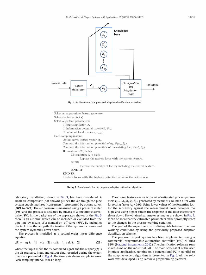
A block diagram depicting the structure of the proposed adap-tive classification scheme is presented in Fig. 1.

The ‘‘feature generator’’ block provides at each sampling instantthe current feature vector zk. The circle nodes represent the compu-tation of the weighted information potential of the current featurevector and of the current focal points inside the knowledge basewith respect to the current historical feature set Zk. The ‘‘classifica-tion and adaptation logic’’ block selects the active focus accordingto the previously described procedure (23) and at the same time ad-justs the knowledge base by replacing or adding focal points wheneither the previously introduced relation (25) or (26) is met.

A pseudo-code of the algorithm is given by next Listing 1. Noticethat the information potentials of the existing foci and of the cur-rent feature vectors are computed recursively according to the pro-cedures described in the Theorems 1 and 2.

3.5. Adaptive expert system for fault detection

The overall architecture of the fault detection expert systemwith ‘‘novelty detection’’ capabilities is presented in Fig. 2. The coreof the system is the previously described adaptive classificationprocedure that modifies, whenever appropriate, the knowledgebase of the algorithm. The appropriate feature generator is prob-lem specific and should be carefully selected case by case. In mostsituations, estimated parameter values of a suitably chosen linearprocess model might be adequate and a Kalman filter could beused in that case as the feature generator. It is worth noting thatKalman filters of various type are often used as residual generatorsin fault detection strategies. Among some recent examples, thereader is referred to Karami et al. (2010), Villeza et al. (2011),and Chinniah et al. (2006).

In the initialization phase, expert knowledge should be used toappropriately select the initial focal points. This initialization pro-cedure is however not obligatory as the proposed classificationalgorithm might be also started with a dummy selection of the ini-tial focal points thanks to its ‘‘learning’’ capabilities. This fact is la-ter put into evidence in the framework of experimental verificationof the suggested methodology, where, in fact, the knowledge basewill be initialized with a dummy focus.

Each focal points corresponds to a specific working condition ofthe plant under consideration. Due to non-linearity of the realplants, it might be possible to assign multiple focal points to a spe-cific working condition. In this case, it might be unrelevant for FDIpurposes to distinguish between the multiple focal points associ-ated to the same working condition.

Working conditions should be roughly classified in a number ofcategories. Nominal working conditions are those which are ex-pected to occur during normal process operation. Faulty conditionsare those corresponding to unwanted behaviour and faults. How-ever, a number of other categories may be introduced. For example,some faulty conditions may be labelled as fatal, corresponding toworking conditions which completely degrade plant performanceor to faults which would result in unsafe operations.

The knowledge base also contains a detailed description of eachworking condition. For the faulty conditions (either of fatal or nonfatal type) such description also contains relevant instructions forthe operator. Each time a new focal point is introduced, a domainexpert must be consulted to label it and provide a suitable descrip-tion. Obviously, this process can not be automated.

4. Experimental verification

To test the proposed methodology using real measurementsrather than computer-generated synthetic ones, a pneumatic

kzkz

*1z

*2z

*3z

*Mz

Fig. 1. Architecture of the proposed adaptive classification procedure.

Listing 1. Pseudo-code for the proposed adaptive estimation algorithm.

M. Petkovic et al. / Expert Systems with Applications 39 (2012) 10226–10235 10231

laboratory installation, shown in Fig. 3, has been considered. Asmall air compressor (not shown) pushes the air trough the pipesystem supplying three ‘‘consumers’’ represented by output valves(OV1 to OV3). The air pressure is measured using a pressure meter(PM) and the process is actuated by means of a pneumatic servo-valve (SV). In the backplane of the apparatus shown in the Fig. 3there is an air tank, which can be included or excluded from thepipe line by means of a manual on–off valve (MV). By includingthe tank into the air path the inertia of the system increases andthe system dynamics slows down.

The process is modelled as a second order linear differenceequation

y½k� ¼ �ay½k� 1� � y½k� 2� þ cu½k� 1� þ du½k� 2�; ð28Þ

where the input u(t) is the SV command signal and the output y(t) isthe air pressure. Input and output data recorded during the exper-iment are presented in Fig. 4. The time axis shows sample indexes.Each sampling interval is 0.1 s long.

The chosen feature vector is the set of estimated process param-eters zk ¼ ðak; bk; ck; dkÞ, generated by means of a Kalman filter withforgetting factor kkf = 0.99. Using lower values of the forgetting fac-tor the sensitivity against the measurement noise becomes toohigh, and using higher values the response of the filter excessivelyslows down. The obtained parameter estimates are shown in Fig. 5.It can be seen that the estimated parameters rather promptly reactto the changes in the process working condition.

The goal of the experiment is to distinguish between the twoworking conditions by using the previously proposed adaptiveclassification scheme.

The proposed expert system has been implemented using acommercial programmable automation controller (PAC) NI cRIO9204 (National instruments, 2012). The classification software runsin real-time on the industrial PAC. The main screenshot of the userinterface application, running on a conventional PC in parallel tothe adaptive expert algorithm, is presented in Fig. 6. All the soft-ware was developed using LabView programming platform.

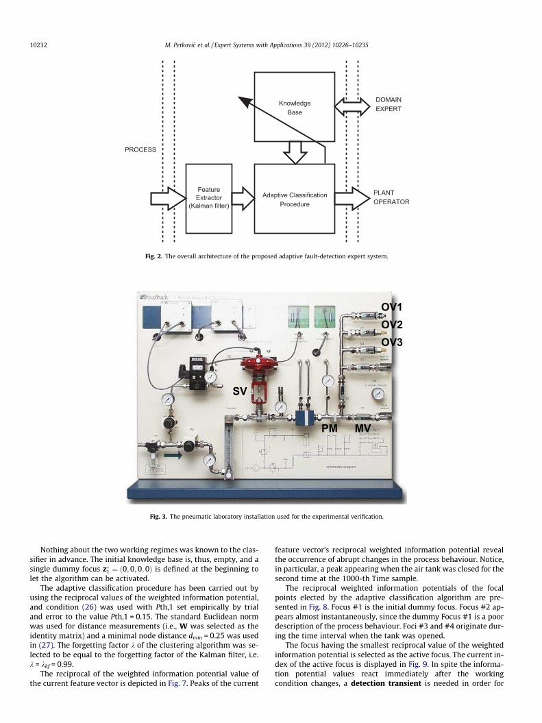
Fig. 2. The overall architecture of the proposed adaptive fault-detection expert system.

Fig. 3. The pneumatic laboratory installation used for the experimental verification.

10232 M. Petkovic et al. / Expert Systems with Applications 39 (2012) 10226–10235

Nothing about the two working regimes was known to the clas-sifier in advance. The initial knowledge base is, thus, empty, and asingle dummy focus z�1 ¼ ð0;0;0;0Þ is defined at the beginning tolet the algorithm can be activated.

The adaptive classification procedure has been carried out byusing the reciprocal values of the weighted information potential,and condition (26) was used with Pth,1 set empirically by trialand error to the value Pth,1 = 0.15. The standard Euclidean normwas used for distance measurements (i.e., W was selected as theidentity matrix) and a minimal node distance dmin = 0.25 was usedin (27). The forgetting factor k of the clustering algorithm was se-lected to be equal to the forgetting factor of the Kalman filter, i.e.k = kkf = 0.99.

The reciprocal of the weighted information potential value ofthe current feature vector is depicted in Fig. 7. Peaks of the current

feature vector’s reciprocal weighted information potential revealthe occurrence of abrupt changes in the process behaviour. Notice,in particular, a peak appearing when the air tank was closed for thesecond time at the 1000-th Time sample.

The reciprocal weighted information potentials of the focalpoints elected by the adaptive classification algorithm are pre-sented in Fig. 8. Focus #1 is the initial dummy focus. Focus #2 ap-pears almost instantaneously, since the dummy Focus #1 is a poordescription of the process behaviour. Foci #3 and #4 originate dur-ing the time interval when the tank was opened.

The focus having the smallest reciprocal value of the weightedinformation potential is selected as the active focus. The current in-dex of the active focus is displayed in Fig. 9. In spite the informa-tion potential values react immediately after the workingcondition changes, a detection transient is needed in order for

Fig. 4. Process input and output signals.

Fig. 5. Estimates of the process parameters. Outputs of the Kalman filter.

Fig. 6. A screen-shot of the user interface application.

M. Petkovic et al. / Expert Systems with Applications 39 (2012) 10226–10235 10233

the focal point corresponding to the actual working regime to be-come the active one. This transient (highlighted in the Fig. 9) takesabout 300 samples, in the first transition from the tank closed toopen condition, and about 200 samples in the successive operating

mode transition from open to closed tank. It seems natural,therefore, to associate Focus #2 with the closed tank working con-dition, and both Foci #3 and #4 with the open tank processcondition.

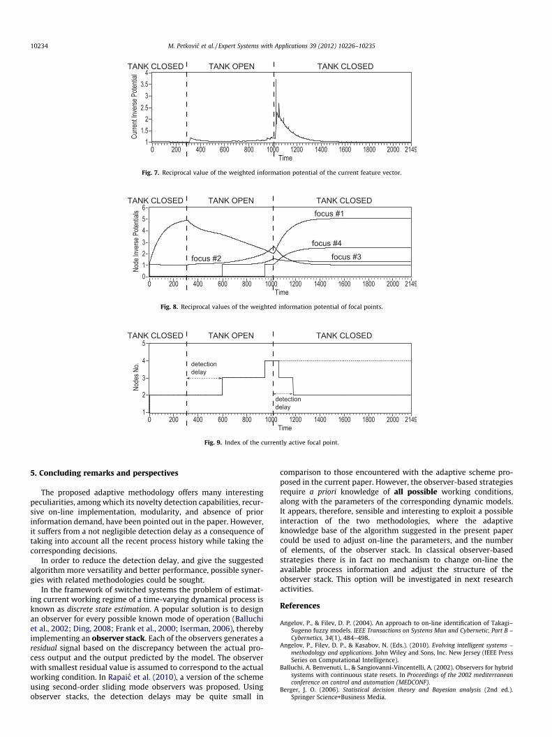
Fig. 7. Reciprocal value of the weighted information potential of the current feature vector.

Fig. 8. Reciprocal values of the weighted information potential of focal points.

Fig. 9. Index of the currently active focal point.

10234 M. Petkovic et al. / Expert Systems with Applications 39 (2012) 10226–10235

5. Concluding remarks and perspectives

The proposed adaptive methodology offers many interestingpeculiarities, among which its novelty detection capabilities, recur-sive on-line implementation, modularity, and absence of priorinformation demand, have been pointed out in the paper. However,it suffers from a not negligible detection delay as a consequence oftaking into account all the recent process history while taking thecorresponding decisions.

In order to reduce the detection delay, and give the suggestedalgorithm more versatility and better performance, possible syner-gies with related methodologies could be sought.

In the framework of switched systems the problem of estimat-ing current working regime of a time-varying dynamical process isknown as discrete state estimation. A popular solution is to designan observer for every possible known mode of operation (Balluchiet al., 2002; Ding, 2008; Frank et al., 2000; Iserman, 2006), therebyimplementing an observer stack. Each of the observers generates aresidual signal based on the discrepancy between the actual pro-cess output and the output predicted by the model. The observerwith smallest residual value is assumed to correspond to the actualworking condition. In Rapaic et al. (2010), a version of the schemeusing second-order sliding mode observers was proposed. Usingobserver stacks, the detection delays may be quite small in

comparison to those encountered with the adaptive scheme pro-posed in the current paper. However, the observer-based strategiesrequire a priori knowledge of all possible working conditions,along with the parameters of the corresponding dynamic models.It appears, therefore, sensible and interesting to exploit a possibleinteraction of the two methodologies, where the adaptiveknowledge base of the algorithm suggested in the present papercould be used to adjust on-line the parameters, and the numberof elements, of the observer stack. In classical observer-basedstrategies there is in fact no mechanism to change on-line theavailable process information and adjust the structure of theobserver stack. This option will be investigated in next researchactivities.

References

Angelov, P., & Filev, D. P. (2004). An approach to on-line identification of Takagi–Sugeno fuzzy models. IEEE Transactions on Systems Man and Cybernetic, Part B –Cybernetics, 34(1), 484–498.

Angelov, P., Filev, D. P., & Kasabov, N. (Eds.). (2010). Evolving intelligent systems –methodology and applications. John Wiley and Sons, Inc. New Jersey (IEEE PressSeries on Computational Intelligence).

Balluchi, A. Benvenuti, L., & Sangiovanni-Vincentelli, A. (2002). Observers for hybridsystems with continuous state resets. In Proceedings of the 2002 mediterraneanconference on control and automation (MEDCONF).

Berger, J. O. (2006). Statistical decision theory and Bayesian analysis (2nd ed.).Springer Science+Business Media.

M. Petkovic et al. / Expert Systems with Applications 39 (2012) 10226–10235 10235

Chinniah, Y., Burton, R., & Habibi, S. (2006). Failure monitoring in a highperformance hydrostatic actuation system using the extended Kalman filter.Mechatronics, 16, 643–653.

Ding, S. X. (2008). Model-based fault diagnosis techniques. Berlin Heidelberg:Springer-Verlag.

Frank, P. M., Ding, S. X., & Marcu, T. (2000). Model-based fault diagnosis in technicalprocesses. Transactions of the Institute of Measurements and Control, 22(1),57–101.

Iserman, R. (2006). Fault-diagnosis systems – An introduction from fault detection tofault tolerance. Berlin Heidelberg: Springer-Verlag.

Izenman, A. J. (2008). Modern multivariate statistical techniques: regression.Classification and manifold learning. Springer Science+Business Media.

Kanovic, Z., Rapaic, M. R., & Jelicic, Z. D. (in press) Generalized particle swarmoptimization algorithm – Theoretical and empirical analysis with application infault detection, Applied Mathematics and Computation. doi:10.1016/j.amc.2011.05.013.

Karami, F., Poshtan, J., & Poshtan, M. (2010). Detection of broken rotor bars ininduction motors using nonlinear Kalman filters. ISA Transactions, 49, 189–195.

Kecman, V. (2001). Learning and soft computing: support vector machines, neuralnetworks, and fuzzy logic models. MIT Press.

Love, J. (2007). Process automation handbook – A guide to theory and practice.Springer-Verlag London Limited.

Markou, M., & Singh, S. (2003a). Novelty detection: A review – Part 1: Statisticalapproaches. Signal Processing, 83(12), 2481–2497.

Markou, M., & Singh, S. (2003b). Novelty detection: A review – Part 2: Neuralnetwork based approaches. Signal Processing, 83(12), 2499–2521.

Matic, D., Kulic, F., Pineda-Sánchez, M., & Kamenko, I. (2012). Support vectormachine classifier for diagnosis in electrical machines. Application to brokenbar, Expert Systems with Applications. doi:10.1016/j.eswa.2012.01.214.

Mendonca, L. F., Sousa, J., & da Costa, J. S. (2009). An architecture for fault detectionand isolation based on fuzzy models. Expert Systems with Applications, 36,1092–1104.

National instruments, (2012). NI CompactRIO developers guide. <http://www.ni.com/compactriodevguide/>.

Quian, Y., Li, X., Jiang, Y., & Wen, Y. (2003). An expert system for real-time fault diagnosys**of complex chemical processes. Expert Systems with Applications, 24, 425–432.

Rapaic, M., Jelicic, Z., Pisano, A., & Usai, E. Second-order sliding modes and softcomputing techniques for fault detection. In Proceedings of the 8th europeanworkshop on advanced control and diagnosis (ACD 2010) (pp. 271–277).

Schölkopf, B., & Smola, A. J. (2002). Learning with kernels. MIT Press.Tang, J.-Z., & Wang, Q.-F. (2008). Inline fault diagnosys and prevention expert

system for dredgers. Expert Systems with Applications, 34, 511–521.Venkatasubramanian, V., Rangaswami, R., & Kavuri, S. N. (2003b). A review of

process fault detection and diagnosis Part II: Quantitative models and searchstrategies. Computers and Chemical Engineering, 27, 213–326.

Venkatasubramanian, V., Rangaswami, R., Yin, K., & Kavuri, S. N. (2003a). A review ofprocess fault detection and diagnosis Part I: Quantitative model-basedmethods. Computers and Chemical Engineering, 27, 293–311.

Venkatasubramanian, V., Rangaswami, R., Yin, K., Kavuri, S. N., & Yin, K. (2003c). Areview of process fault detection and diagnosis part III: Process history basedmethods. Computers and Chemical Engineering, 27, 327–346.

Villeza, K., Srinivasanb, B., Rengaswamyb, R., Narasimhanc, S., &Venkatasubramanian, V. (2011). Kalman-based strategies for fault detectionand identification (fdi): Extensions and critical evaluation for a buffer tanksystem. Computers and Chemical Engineering, 35, 806816.

White, C. J., & Lakany, H. (2008). A fuzzy interface system for fault detection andisolation: Application to fluid system. Expert Systems with Applications, 35,1021–1033.