Embed Size (px)
Citation preview
Expert knowledge in geostatistical
inference and prediction
Phuong Ngoc Truong
Thesis committee
Promotor
Prof. Dr P.C. de RuiterPersonal chair at BiometrisWageningen University
Co-promotor
Dr G.B.M. HeuvelinkAssociate professor, Soil Geography and Landscape GroupWageningen University
Other members
Dr S. de Bruin, Wageningen UniversityProf. Dr C. Kroeze, Wageningen University
Prof. Dr F.D. van der Meer, University of Twente, Enschede
This research was conducted under the auspices of the C.T. de Wit Graduate School Production Ecology & Resource Conservation.

Thesis
at Wageningen University
Prof. Dr M.J. Kropff,in the presence of the
Thesis Committee appointed by the Academic Boardto be defended in publicon Monday 30 June 2014at 1:30 p.m. in the Aula.
Expert knowledge in geostatistical
inference and prediction
Phuong Ngoc Truong

Phuong Ngoc Truong
Expert knowledge in geostatistical inference and prediction,
160 pages.
PhD thesis, Wageningen University, Wageningen, NL (2014)
With references, with summaries in Dutch, Vietnamese and English
ISBN: 978-94-6257-028-3

Chapter 1 General introduction 1.1. Geostatistics and expert knowledge 8 1.2. Statistical expert elicitation for spatial phenomena 12 1.3. Research objectives 12
1.5. Scope and expected contributions of the dissertation 15
Chapter 2 Web-based tool for expert elicitation of the variogram 2.1. Introduction 18 2.2. Developing a statistical expert elicitation protocol 21 2.3. Description of the web-based tool 27 2.4. Illustrative example 29 2.5. Discussion and Conclusions 34
Chapter 3with statistical expert elicitation
3.1. Introduction 40 3.2. Materials and methods 42 3.3. Results 47 3.4. Discussion and Conclusions 59 Appendix 3.A. Questionnaire for elicitation exercise evaluation 63
Chapter 4 Bayesian area-to-point kriging using expert knowledge as informative priors
4.1. Introduction 68 4.2. Materials and Methods 71 4.3. Results and Discussion 77 4.4. Conclusions and Recommendations 88
Contents

Chapter 5 Incorporating expert knowledge as observations in
with regression cokriging 5.1. Introduction 92 5.2. Methods 94 5.3. Case study 97 5.4. Results and Discussion 104 5.5. Conclusions 110 Appendix 5.A. Soil condition and expert judgements at 50 locations 111 Appendix 5.B. Locations of sampling scheme for expert elicitation 113
Chapter 6 General discussion 6.1. Introduction 116 6.2. What is the role of expert knowledge in 117
geostatistical inference and prediction? 6.3. How to elicit and incorporate expert knowledge in 120
geostatistical inference and prediction? 6.4. Insight and Implications 125 6.5. Conclusions 127
References 129
Summary 143
Samenvatting 147
151
Publications 155

General introduction
Chapter 1

8 CHAPTER 1
1 1.1. Geostatistics and expert knowledge
1.1.1. Geostatistics
Geostatistics is originally the study of the spatial distribution of natural resources in mining and geology (Matheron, 1963), where the statistical modelling of spatial dependence is used for inference of spatial structure and for spatial prediction at unobserved locations from observations (i.e. kriging prediction). These are the two main purposes of geostatistical analysis. It has also founded an important statistical
kriging variance.
A geostatistical model represents a spatial phenomenon as a regionalised var-iable whose mean may depend on explanatory environmental variables and whose spatial dependence is modelled by the variogram. When the variation of the spa-tial phenomenon shows an obvious trend, the geostatistical model is the sum of the spatial trend (i.e. spatial mean) that models the large scale variation and the ze-ro-mean random residual. The spatial trend can be modelled as a (unknown) constant or a linear function of the covariates (i.e. the predictive secondary variables). The zero-mean random residual models the small scale variation (including small-scale, microscale and white-noise variation) and is characterised by the variogram (Cressie, 1991, Section 3.1). The variogram is a mathematical function that plots the semivar-
the differences of the variable at two locations a certain distance apart (Armstrong, 1998; Oliver and Webster, 2014). Geostatistical data have a continuous variation in geographical space, but can be discontinuous in attribute space (Cressie, 1991, Section 1.2.1; Schabenberger and Gotway, 2005, Section 1.2.1).
In this dissertation, geostatistical inference refers to estimation of the vari-
prediction refers to prediction of the spatial variables at unobserved locations. In general, the geostatistical prediction or kriging prediction at an unobserved location is a weighted avarage of the surrounding observations (Cressie, 1990; Stein, 1999). In
weighted average of the trend residuals at the surrounding observed locations. The

GENERAL INTRODUCTION 9
1
magnitude of the kriging weights are controlled by the spatial dependence between the unobserved locations and the surrounding observations, and they guarantee unbi-asedness and minimise the kriging variance (i.e., provide the ‘best’ predictor).
Geostatistics has been applied in various disciplines of the Earth and envi-ronmental sciences, such as geology, hydrology, soil science, ecology, forestry and climatology. Kriging tools can produce exhaustive maps of the spatial phenomena
soil pollutions or ambient air pollutions are needed to assess public exposure to these pollutions that can help prevent public health problems. Recently, mapping of spatial variation of epidemics using geostatistics proves useful in accessing the relationship between disease incidence and environmental, social-demographic factors. There are
and societal value of geostatistics.
1.1.2. The challenges of optimal use of data for geostatistical inference and
prediction
Geostatistical inference and prediction are fundamentally dependent on observations
-uously varies over a certain spatial domain, the observations can be sampled every-where within this spatial domain for spatial inference. However, very often, the ob-servations used in geostatistics are only a limited sample of locations (point support) or areas (block support). Moreover, the number of sampling locations is often con-
and environmental impact of sampling. These constraints may lead to unsatisfactory sampling density and unrepresentativeness of the observations that can hinder the effective use of geostatistics in spatial inference and prediction.
Geostatisticians are well aware of the possible drawbacks of using limited ob-servations in geostatistical inference and prediction. Considerable research has studied the magnitude of this effect on the accuracy of geostatistical inference and prediction (e.g. McBratney and Webster, 1983; Webster and Oliver, 1992; Frogbrook, 1999; Oli-

10 CHAPTER 1
1 ver and Webster, 2014). Meanwhile, various methods have been developed to increase the accuracy of geostatistical inference and prediction. For example, optimum sam-pling schemes are recommended to reduce kriging variance (McBratney et al., 1981; van Groenigen et al., 1999; Brus and Heuvelink, 2007; Vasát et al., 2010) and to best use the observations for variogram inference (Warrick and Myers, 1987; Lark, 2002;
statistical algorithms for variogram estimation are recommended such as maximum
to reach a comparable estimation accuracy.
Geostatisticians have also incorporated different types of data and informa-tion in geostatistical models to improve the mapping accuracy. The terms prior in-formation, soft data, secondary information or ancillary data have been used in the geostatistical literature to indicate data or information other than direct (error-free) measurements of the target variable itself (Stein, 1994; Goovaerts, 1997, Chapter 6; Kerry and Oliver, 2003; Oliver et al., 2010b). The use of extra data and information is certainly valuable in many geostatistical applications. For example, optimal sampling design needs prior information about the spatial variation in a certain area before measurements are collected (Kerry and Oliver, 2004). Spatially exhaustive ancillary
correlation between temperature and elevation furnishes the use of elevation as an external drift variable to make a better prediction (Hudson and Wackernagel, 1994). Kriging tools such as regression kriging, cokriging, Bayesian kriging and indicator (co)kriging have been used to incorporate these different sources of data and information (Hoef and Cressie, 1993; Hudson and Wackernagel, 1994; Goovaerts, 1997, Chapter
1.1.3. The concept of expert knowledge in geostatistics
While ancillary data and information are often used as an additional source of data and information in modern geostatistics, expert knowledge about spatial phenome-na is a huge pool of knowledge that is relatively unnoticed. A study of Stein (1994) gives an early overview of the use of ancillary information as prior information (i.e.
GENERAL INTRODUCTION 11
1
interpolation, and expert knowledge has been mentioned as one option. A large body of expert knowledge about spatial phenomena has been accumulated in various dis-ciplines of the Earth and environmental sciences.
Aforementioned, geostatistics characterises spatial variables by the spatial trend and the variogram. In case of multiple variables, there are also cross-variograms that
expert knowledge for geostatistical research is essentially about these trends and spa-tial correlations. For example, experienced pedologists have good knowledge about the relationships between soils and environmental variables such as soil forming fac-tors (parent material, climate, vegetation, rainfall, etc.). A study of Walter et al. (2006) gives an overview of the origin of expert knowledge in pedology. Expert knowledge
-ster and Oliver, 2007) and to best guess or ‘guesstimate’ the magnitude of spatial correlations (Kros et al., 1999). However, systematic use of expert knowledge has
be used as soft-information in mapping soil texture (Oberthür et al., 1999), to guide spatial sampling design according to expert judgements about the spatial variation of a certain variable in a certain area (van Groenigen et al., 1999), to supplement sparse observations for spatial inference (Lele and Das, 2000), or to specify the spatial rela-tionship between the target variable and the covariates to develop optimum models for spatial prediction (Lark et al., 2007).
All studies that make use of or refer to expert knowledge show a great potential of using expert knowledge in geostatistics. But these studies also show that expert knowledge has not been formally and systematically used in geostatistical modelling and mapping. The use of expert knowledge has also been criticised or undervalued because expert knowledge that is transformed into expert judgement is considered subjective and intractable (Tversky and Kahneman, 1974; Meyer and Booker, 2001, Chapter 2; O’Hagan et al., 2006, Chapter 3; McKenzie et al., 2008). This might be
previous studies that use expert knowledge, the description of how expert knowledge is elicited is overlooked.

12 CHAPTER 1
1 1.2. Statistical expert elicitation for spatial phenomena
Several common expressions are often encountered in the statistical expert elicitation literature and also in this dissertation: expert, expert knowledge, expert judgement or
on a subject matter (e.g. scientist, professional or experienced practitioner). Expert -
titative statements. Expert knowledge is extracted into expert judgement or expert opinion (e.g. a meteorologist’s estimate of the difference in average temperature in 2013 between Amsterdam, The Netherlands and Ohio, The United States, an econo-
There is no distinction between these two terms. Expert data in this dissertation refers
-
statistical expert elicitation is a systematic process of formulating expert knowledge
Because statistical expert elicitation is a systematic process, it involves several stag-
and revision, documentation and reporting (O’Hagan et al., 2006; Choy et al., 2009; Knol et al., 2010; Kuhnert et al., 2010). Depending on the purpose of the research,
-
to reach consensus among experts (French, 2011). Statistical expert elicitation is an appropriate approach to capture expert knowledge about the regionalised variables that represent spatial phenomena in geostatistics. To my knowledge, statistical expert elicitation has never been used to elicit expert knowledge to model spatial phenome-
expert elicitation research, I assert that expert knowledge can be elicited and used in a responsible and defensible way for geostatistical inference and prediction.
1.3. Research objectives

GENERAL INTRODUCTION 13
1
and accordingly, to identify the use of expert knowledge in geostatistical inference and prediction. The second is to investigate how to elicit expert knowledge and incor-porate expert knowledge in geostatistical models for spatial inference and prediction.
1.4. Research questions and dissertation outline
1.4.1. Main research questions
main research objectives:
1. What is the role of expert knowledge in geostatistical inference and prediction?
2. How to elicit and incoporate expert knowledge in geostatistical inference and pre-diction?
-
1.4.2. Detailed research questions
to 5 are:
1. How to apply statistical expert elicitation to elicit the variogram from multiple ex-perts’ knowledge?
The variogram is the keystone of geostatistics. Almost half of the effort in geostatistical research is spent on estimation of the variogram. Practically, all applied research in geostatistics makes use of the variogram. Chapter 2 of this dissertation
were applied to elicit from multiple experts probabilistic judgements that can be used to estimate the variogram. The intention of applying statistical expert elicitation tech-
-
1.1. Which measure to infer the variogram can be elicited from experts?

14 CHAPTER 1
1 experts the selected measure?
1.3. How to combine multiple expert judgements?
1.4. Is developing an online statistical expert elicitation tool an effective ap-proach?
One important reason for using kriging in spatial mapping is that it provides un-
used in all spatial mapping exercises. For instance, many soil maps have been derived by other ways (e.g. using pedotransfer function, aerial photographs, manual drawing
of these maps need to know how accurate they are. I tackled this issue in Chapter 3, where I applied the tool for expert elicitation of the variogram developed in Chapter 2. Question 1.4 is again addressed in Chapter 3, together with the following research
2.1. How to apply the web-based expert elicitation tool for the variogram to
property maps?
3. How to use expert judgements to solve the ill-posed problem in spatial disaggrega-tion using area-to-point kriging?
An important research topic in geostatistics is the change of support problem. Here, the (spatial) support refers to the area or volume over which a measurement or a prediction is made. Geostatistics may be confronted with the problem of spatial disaggregation when the support of the observations is larger than that of the pre-dictions (e.g. using remote sensing imagery or choropleth maps as observations for mapping the continuous variation over a spatial domain). In Chapter 4, this problem
3.1. Why is the nugget parameter of the point support variogram often ignored in variogram deconvolution?
3.2. How to incorporate expert judgements in block support data to infer the
GENERAL INTRODUCTION 15
1
point support variogram model?
-eter uncertainty) and model uncertainty propagation to spatial disaggregation?
4. How to incorporate expert judgements as observations in geostatistical inference and prediction?
Finally, I address a very conventional issue in geostatistics, which I have also discussed in Section 1.1. This is that in many geostatistical analyses, there is a lack of observations. Chapter 5 addresses the use of expert knowledge as inaccurate obser-
in Chapter 5 are:
4.1. How to measure bias and imprecision of expert probabilistic judgements
data?
4.2. How to incorporate expert judgements as observations to characterise spa-tial variation using the variogram?
4.3. Which kriging method can be used to incorporate expert data in spatial prediction?
1.5. Scope and expected contributions of the dissertation
1.5.1. Scope of the dissertation
Mapping spatial variation of natural phenomena using expert knowledge is the main focus of my research; the spatio-temporal aspect of natural phenomena in geostatis-tics is not touched. Four illustrative examples and case studies presented in Chapters 2 to 5 are:
1. mapping of air temperature over The Netherlands;
Anglian Chalk area, The United Kingdom;
3. mapping air temperature over the Gelderland province, The Netherlands us-ing remote sensing imagery;

16 CHAPTER 1
1 a study area in the Malpiebeemden nature reserve in the south of The Nether-lands.
All experts who were involved in this research are scientists (i.e. professors and
such as soil science, hydrology and meteorology.
In the next four chapters, expert knowledge was always elicited in probabilistic
elicitation was employed to build the elicitation tools. A model-based perspective in geostatistics (Diggle and Ribeiro, 2007) was taken as a foundation to develop the models to incorporate expert knowledge in geostatistical inference and prediction.
1.5.2. Expected contributions
-edge in geostatistical research and the opportunity to enhance the use of expert
in the four main focuses of geostatistical research: variogram estimation, spatial un-
solutions for the elicitation approaches and incorporation methods of expert knowl-edge in these geostatistical research focuses are provided. Chapter 6 concludes the
I have done and what can be done in the future to advance this research topic. This dissertation as a whole may contribute to the optimum use of data and information, both derived from measurements and from experts, for geostatistical inference and prediction. It may help advance the understanding of the Earth surface and subsur-face spatial phenomena.
Web-based tool for expert elicitation
of the variogram
Based on: Truong, P.N., Heuvelink, G.B.M., Gosling, J.P., 2013. Computers & Geo-sciences 51, 390-399.
Chapter 2

18 CHAPTER 2
22.1. Introduction
Geostatistical interpolation of environmental variables from georeferenced observa-
spatial variability of environmental variables is characterized by the variogram (Jour-
Oliver, 2007). Theory about the variogram and kriging is well-described in the geosta-tistical literature. We only recall that the variogram is commonly modelled from the empirical or sample variogram that is estimated from available observations using the common Matheron method-of-moments (Matheron, 1963). A dominant factor that controls the accuracy of the variogram estimate is the number of observations. Web-ster and Oliver (2007) recommend using at least 100-150 observations for estimating the isotropic variogram and at least 250 observations for the anisotropic variogram.
-pensive and time-consuming. There have been attempts to increase the accuracy of the variogram estimate for a given number of observations by using different statis-
provide an alternative to the method-of-moments when there are fewer than 100 ob--
ence for estimation of the variogram parameters and their uncertainty by combining hard measurements with soft data from available prior information.
Environmental scientists are increasingly aware of the use of prior information of spatial variation in cost-effective sampling design for both variogram estimation (Cui et al., 1995; Lark, 2002; Kerry and Oliver, 2007) and optimum spatial interpola-tion (McBratney and Pringle, 1999; Kerry and Oliver 2003, 2004; Brus and Heuvelink, 2007). In addition, Bayesian inference of environmental variables making use of prior information of spatial variation has also become popular in mapping spatial varia-bles with small samples, e.g. mapping hydrodynamic variables or petroleum reservoirs
research on the use of objective prior information for variogram estimation is the use of a (average) variogram derived from a similar study area (Cui et al., 1995; McBratney and Pringle, 1999; Kerry and Oliver, 2004) or using a variogram derived from ancil-

EXPERT ELICITATION FOR THE VARIOGRAM 19
lary data (Kerry and Oliver, 2003). These approaches rely on the similarity of spatial variation between similar areas and situations, which may not always be realistic or available. Alternatively, the value of subjective prior knowledge when available data are scarce or unreliable has been acknowledged recently in landscape ecology, geo-sciences and geographical research (Denham and Mengersen, 2007; James et al., 2010; Curtis, 2012; Perera et al., 2012a).
There are obvious demands for prior information about the spatial variation of
to guide optimum sampling designs for costly measured and analysed variables. The
information for inference when data are limited due to budget constraints or physi-
2012). In such cases, experts can be an important source of information because ex-perts can be very knowledgeable about the spatial variability of a variable of interest. Expert knowledge is also important when no data are available to predict the future variation in spatial pattern (e.g. patterns of temperature or ozone concentration over a region ahead of time). We therefore suggest that consulting experts may be sensi-
from expert knowledge in a responsible way. In previous research (Kros et al., 1999), the spatial correlations of continuous variables are simply ‘guestimated’ by deriving a spatial correlation structure from direct consultation of experts. In this study, we
rules from statistical expert elicitation.
From a statistical perspective, statistical expert elicitation is the process of
knowledge about some aspects of the problem that the analysts want to elicit (Meyer and Booker, 2001; Garthwaite et al., 2005). Examples of typical cases that need expert assessment are estimation of new, rare, complex or poorly understood phenomena, future forecasts for particular events, interpretation of existing data, group decision making or extracting the current state of knowledge about certain phenomena (Meyer and Booker, 2001). The ultimate purpose of statistical expert elicitation is to reliably and consistently encode a person’s knowledge or belief about an uncertain variable

20 CHAPTER 2
2as a probability distribution (in general, expert elicitation may not necessarily need to encode expert knowledge using a probability distribution).
Formal statistical expert elicitation procedure involves a systematic process with several stages (O’Hagan et al., 2006; Choy et al., 2009; Knol et al., 2010; Kuhnert et
Before conducting the elicitation, experts should be motivated and trained through a dry-run. Execution of the elicitation process can be done in a workshop of a group of experts with support of computer software and must be facilitated by the analysts. It can also be an individual elicitation by means of face-to-face interviews, online or telecom interviews. The analysts play an important role in this stage: they have the re-sponsibility of facilitating, designing or choosing elicitation protocols and supporting tools. Expert judgement is encoded into probability distributions by either parametric
to experts, commonly in graphical forms and letting experts revise their judgements if needed. Elicited information from multiple experts can be combined by a mathe-matical pooling approach (O’Hagan et al., 2006). Bringing experts together in group elicitation is another way of obtaining consensual judgments, in this case using the so-called behavioural approach (O’Hagan et al., 2006). Heuristics and biases in expert cognition may result in inaccurate probability judgements (Kynn, 2008). The struc-tured elicitation protocol has been designed in an attempt to minimize all contamina-tions to the process of eliciting reliable expert judgement.
Statistical expert elicitation functions as a statistical tool to extract knowledge from experts about real-world phenomena. In practice, statistical expert elicitation procedure needs computer assistance to effectively, conveniently and routinely cap-ture and encode expert judgement (O’Hagan, 1998). In response to this, an increasing number of software and web-based tools have been built. Examples of web-based tools for the elicitation of univariate discrete and continuous probability distributions of uncertain variables are the MATCH Uncertainty elicitation tool (Morris et al., 2014) and The Elicitator (UncertWeb - The Elicitator1, assessed 29/02/2012); exam-ples of software are SHELF (Oakley and O’Hagan, 2010) - the elicitation framework for single and multiple experts, Elicitator (James et al., 2010; Low-Choy, 2012) for elicitation of regression models in ecology, and ElicitN (Fisher et al., 2012) for elici-tation of species richness.1 http://elicitator.uncertweb.org
EXPERT ELICITATION FOR THE VARIOGRAM 21
However, so far statistical expert elicitation has not been used to characterise spatial variation and elicit the variogram from experts. In this chapter, we aimed at applying statistical expert elicitation to geostatistical research domain, particularly to elicit the variogram from expert knowledge. We developed a novel and generic statis-tical expert elicitation protocol and built a web-based tool to facilitate statistical expert elicitation for the variogram of an isotropic second-order stationary multivariate nor-
In Section 2.2, we present the statistical expert elicitation protocol. Section 2.3 describes the web-based tool, its architecture and functionality. In Section 2.4, we present the results from a simple case study to test the protocol and web-based tool.
of the tool and avenues for further research in Section 2.5.
2.2. Developing a statistical expert elicitation protocol
-
its estimators that forms the basis for the developed protocol is presented.
Z(s1) – Z(s2)] (Journel and Huijbregts, 1978) where Z is the random function that characterizes the
s1
and s2 s1, s2 Z(s1) – Z(s2)].
Assuming that Z is an isotropic second-order stationary random function on the Z(s1 Z(s2
Z(s1) – Z(s2)] = 0,
h
with hvectors s and s Z(s+h) – Z(s)].
Dowd (1984) introduced a robust estimator of the variogram, which was de-rived from Cressie and Hawkins (1980), based on the median of the absolute value of
2 ˆ Z(s+h) – Z(s 2 (2.1)
22 CHAPTER 2
2-
Z(s+h) – Z(spsychological research and practical expert elicitation exercises have shown that the
most precise and reliable outcomes (Peterson and Miller, 1964; Kadane and Wolfson, 1998; O’Hagan et al., 2006). Using this approach, the variogram can be inferred at
through these estimates in the usual way. In addition, the marginal probability distri-
distribution of the random process Z over a geographical plane is also elicited.
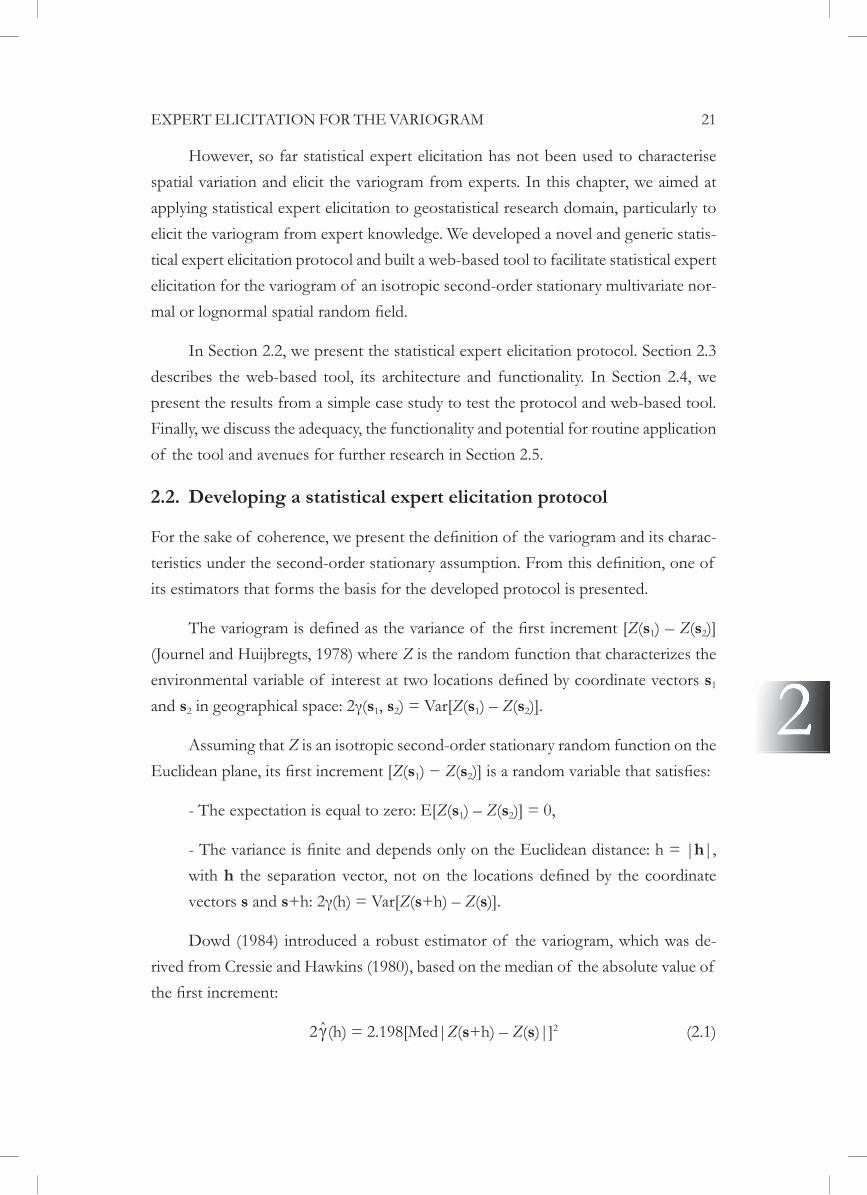
Figure 2.1: Components of elicitation protocol
Based on this concept, the statistical expert elicitation protocol was designed for multiple-expert elicitation with two main rounds. Round 1 is the elicitation for the mpdf and Round 2 is the elicitation for the variogram. Fig. 2.1 outlines the process of the whole elicitation procedure.
2.2.1. Expert elicitation for the marginal probability distribution
To elicit the mpdf, we used the bisection method for unbounded probability distribu--
edge from experts on probability (Garthwaite and Dickey, 1985). Fig. 2.2 outlines the process of Round 1. In this method, the ordered range of possible values of the ran-

EXPERT ELICITATION FOR THE VARIOGRAM 23
dom variable Z(s s is immaterial because Z
Figure 2.2: Round 1 of elicitation procedure
To avoid complexity, it is reasonable to assume that expert’s belief about the mpdf of the random environmental variables can be represented as a normal or log-normal distribution. The decision between normality and lognormality is based on a
(Bowley, 1920):
= (Z0.75 + Z0.25 – 2Zmed)/(Z0.75 – Z0.25) (2.2)
where Z0.25, Zmed, Z0.75
t t, the distribution is assumed the lognormal distribution is assumed.
-

24 CHAPTER 2
2)
and the variance ( 2) of the mpdf are chosen by numerically minimizing:
0.25; , 2) – 0.25]2med; , 2) – 0.5]2
0.75; , 2) – 0.75]2, where F is the normal or lognormal cumulative distribution function.
-liefs are correctly conveyed in the given feedback. Because the mpdf of the random
about the mpdf before proceeding to the next round. Section 2.2.3 details how con-sensus amongst experts can be obtained.
2.2.2. Expert elicitation for the variogram
To model the variogram function, the variogram values for various lags need to be estimated. For kriging, modelling the variogram at small lags is more important than at larger lags because the nearer locations give more weight in the kriging predic-tion (Myers, 1991; Webster and Oliver, 1992, 2007). Choosing more small lags is
-
xmax – xmin)2+(ymax – ymin)2], where xmax, xmin, ymax, ymin
to the nearest number of type k×10a with k=1, 2 or 5 and an integer a (e.g. if the initial distance is 5×10³ then the next is 2×10³, if it is 1×10³ then the next is 5×10², etc.). We chose to elicit from experts the median of no more than seven lags because experience has shown that experts cannot give proper judgements for more than seven values in a single session (Meyer and Booker, 2001). Note also that the ratio of the largest and smallest lag is at least 100 which ensures that the smallest lag is small compared to the extent of the study area.
-mal or lognormal distribution, the next step of eliciting the variogram will be differ-ent. Fig. 2.3 outlines the procedure of Round 2.

EXPERT ELICITATION FOR THE VARIOGRAM 25
Figure 2.3: Round 2 of elicitation procedure
Variogram elicitation in case of the normal distribution
When the consensus mpdf is a normal distribution, Z is a second-order stationary
Z(s + h) – Z(s inc_med for each of the seven lags. The medians elicited from each expert are used to calculate the variograms
mpdf, which is the consensual mpdf from the Round 1 (Barnes, 1991). Thereby, it is easy to derive that the medians judged by experts must satisfy the following condition: Vinc_med 0.75 – Z0.25). This condition is checked during Round 2.
-ulation (Goovaerts, 1997; Pebesma, 2004) along an arbitrary transect within the study area. The variation in simulated values along the transect is shown to the experts. Note that, experts can only see the outcomes from their own judgements. Several simulations are generated and experts can toggle between these to get an impression of the whole range of possible realities. Experts can reconsider whether the spatial structure shown along the transect conveys what they think it should be. If not, they can revise their judgements about the medians at lags and the variogram elicitation is reiterated. Note that at this stage, they can no longer change the judged values of the

26 CHAPTER 2
2Variogram elicitation in case of the lognormal distribution
When the mpdf is lognormal, each expert is asked to judge the median of the absolute ra-tio of change Vr, called Vr_med, between two locations at distance h: Vr Z(s+h)/Z(s
Z(s Z(sZ(s+h)) log(Z(s Z(s+h)/Z(s
Z(s+h)/Z(s Z(s+h)/Z(sthe sill not increasing the variance yields the condition: Vr_med Z0.75/Z0.25)0.709.
-ment of log-transformed values. The remaining steps are the same as in the case of normal mpdf. Note that, because the simulated values in this case are taken from the
values along a transect are shown to experts.
2.2.3. Pooling experts’ judgements
The multiple judgments from experts are combined using the mathematical com-bination method, also known as opinion pooling (O’Hagan et al., 2006). We follow the linear opinion pooling method in which all experts’ judgements are combined by
the elicitation for the mpdf and for the variogram.
The pooling of the mpdf is done by applying probabilistic averaging of many
The minimum value from all experts is taken as the minimum, likewise for the max--
chosen probability distribution (i.e. the normal or lognormal). The consensual mpdf is reported back to each expert, giving them a chance to compare it with their own mpdf and revise their judgements. The process continues until all experts are satis-
point, the Round 1 is ended. In practice, it may be sensible to allow just one revision turn.
To pool the variogram, the medians elicited from all experts for the seven lags -

EXPERT ELICITATION FOR THE VARIOGRAM 27
tation procedure is ended when all experts stop revising their own judged values for the medians.
2.3. Description of the web-based tool
General structure of the web-based tool has three main components: web interface,
design are discussed in detail hereafter.
Figure 2.4: Three main components of web-based tool
2.3.1. Web elicitation interface
The web interface was built around Symfony, which is an Open Source PHP Web application development framework (Symfony, 2012). It facilitates interaction of indi-vidual expert with the tool to automatically proceed through the elicitation procedure.
and answer forms and the graphical feedbacks. Google Maps is embedded to pro-
designed in each webpage with different functions such as saving experts’ judgments, executing statistical computation, rendering graphical feedbacks and navigating.
To access the tool, experts login at URL: http://www.variogramelicitation.org
28 CHAPTER 2
2were set up to handle submission of experts’ judgements. Graphical feedbacks pro-
the Round 2 both for individual and pooled outcomes. The graphical feedbacks are rendered using the Flot - Javascript plotting library2 for jQuery (jQuery3, accessed 28/02/2012).
2.3.2. Database
open source database MySQL. Symfony integrated with Doctrine provides an object 4) to interact with the MyS-
QL database to retrieve and store data.
2.3.3. Statistical computation
variogram, to combine multiple experts’ judgements and to simulate realisations of
combination of the Nugget model with each of the others. The initial parameters
Other statistical functions were originally built around the R package gstat (Pebesma, 2004). All statistical functions were assembled in a standardized format of an R pack-age, named eeVariogram.
Executions of these statistical functions are initialized by experts after they have
-not interfere. PHP executes and passes arguments to R scripts which invoke R func-tions from the eeVariogram package. The outputs are returned to PHP for rendering by Flot.
2 http://www.flotcharts.org/3 4 http://www.doctrine-project.org/

EXPERT ELICITATION FOR THE VARIOGRAM 29
2.4. Illustrative example
set up a simple case study on elicitation of the spatial variability of the maximum tem-perature over The Netherlands on April 1st, 2020. Historical data from KNMI-Royal Netherlands Meteorological Institute were used to compare with the elicitation out-comes. The data are the measured maximum temperature on April 1st from 1993 to 2012 at 35 stations over The Netherlands. Five partners from UncertWeb project5 were invited to join the case study as experts. It should be noted that this simple example was only chosen to test the tool, and that the experts are not climatologists of The Netherlands. Hence, a variable was chosen that, with the right background 5 http://www.uncertweb.org
30 CHAPTER 2
2information provided by the tool, each participant could form an opinion on.
The web-based tool started with information about the geographical attributes, a link to the KNMI website where the experts could obtain information about the weather of the Netherlands and a Google map of The Netherlands. Although the
document, the causes of biased judgements including cognitive bias due to limitations in human information processing and motivational bias due to human subjectivity (Meyer et al., 1990) were also explained to point the experts to possibly major causes of bias in their judgements. The experts were asked to carefully read the introduction
Round 1 and 2.
We present the results from one expert as an example. The expert’s judged val-
past twenty years at an arbitrary selected station shows a fair degree of agreement (Fig. 2.10). Apparently, the experts have a fair idea of the variations that occurred in the past and projected this to assess uncertainty about the maximum temperature on April 1st, 2020.
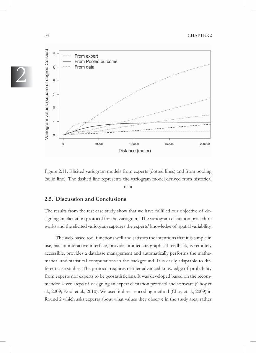
was the Vinc_med. Fig. 2.11 shows the variograms computed from the elicited medians from all experts and the pooled medians at the seven lags (ranging from 2 to 200 km).
knowledge about geostatistics that was not presumed. The pooled variogram model is the Matérn model with nugget = 0.02ºC2, partial sill = 4.56ºC2, range = 27.6 km and smoothness (kappa) = 0.7.

EXPERT ELICITATION FOR THE VARIOGRAM 31

32 CHAPTER 2
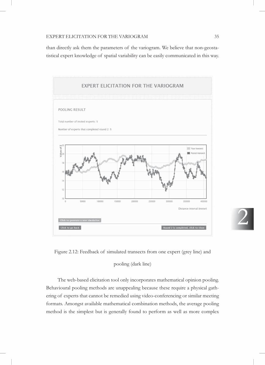
2Fig. 2.12 shows an example of simulation transects that are the actual feedbacks
to the experts. The pooled transect shows a substantial degree of short-distance var-iation; this is in agreement with the pooled variogram model (Fig. 2.11). The vario-gram that was derived from the data over the past twenty years at 35 stations was cal-
model (Fig. 2.11). Although there are data from only 35 stations that make variogram estimation inaccurate, part of this inaccuracy is taken away by pooling over twenty years. By comparison with the variogram model from the data, the elicited variograms from the experts show that the experts tend to overestimate the spatial variability, es-pecially at short distances. This difference may partly be explained by the fact that the experts are indeed not experts in climatology of the Netherlands, partly because the variogram was derived from data of only 35 stations, and partly because the expert elicitation addressed the future temperature.
Figure 2.8: Screenshot of graphical feedback for individual expert’s marginal
probability distribution

EXPERT ELICITATION FOR THE VARIOGRAM 33
Figure 2.9: Screenshot of graphical feedback for pooled marginal probability distri-
bution
Figure 2.10: Histogram of maximum temperature from one station on April 1st over past twenty years compared with experts’ (dotted lines) and pooled (solid line) mar-
ginal probability distribution function
34 CHAPTER 2
2
Figure 2.11: Elicited variogram models from experts (dotted lines) and from pooling (solid line). The dashed line represents the variogram model derived from historical
data
2.5. Discussion and Conclusions
-signing an elicitation protocol for the variogram. The variogram elicitation procedure works and the elicited variogram captures the experts’ knowledge of spatial variability.
use, has an interactive interface, provides immediate graphical feedback, is remotely accessible, provides a database management and automatically performs the mathe-matical and statistical computations in the background. It is easily adaptable to dif-
from experts nor experts to be geostatisticians. It was developed based on the recom-mended seven steps of designing an expert elicitation protocol and software (Choy et al., 2009; Knol et al., 2010). We used indirect encoding method (Choy et al., 2009) in Round 2 which asks experts about what values they observe in the study area, rather
EXPERT ELICITATION FOR THE VARIOGRAM 35
than directly ask them the parameters of the variogram. We believe that non-geosta-tistical expert knowledge of spatial variability can be easily communicated in this way.
Figure 2.12: Feedback of simulated transects from one expert (grey line) and
pooling (dark line)
The web-based elicitation tool only incorporates mathematical opinion pooling. -
ering of experts that cannot be remedied using video-conferencing or similar meeting formats. Amongst available mathematical combination methods, the average pooling method is the simplest but is generally found to perform as well as more complex
36 CHAPTER 2
2approaches (Clemen and Winkler, 1999).
To minimize common biases in expert judgments, especially cognitive bias which occurs more often in a web-based elicitation process, we followed the guide-lines in Meyer et al. (1990) and Choy et al. (2009) in the design of the protocol. The
-perts can encounter. Well-documented information about the study area and related
much as possible, while revision of judgements is allowed to further reduce anchoring -
nology to prevent misunderstandings. Question forms of both rounds have no more -
ity. Motivational bias is limited in real time, e.g. experts are not informed about other experts and their individual judgements. The indirect encoding method used does not directly show a link between the experts’ answers and the encoded variogram param-
interpretations.
The web-based tool presented in this work is a research prototype that has sev-eral limitations. Firstly, the feedback of the simulated transect in Round 2 was found
of multiple simulated maps over whole study area, although this can slow down the
accuracy. This can frustrate experts to spend much time on the revision. However,
some IT skills that might limit the easy reuse of the tool. Implementation of a user interface to conveniently create different case studies (for example, see The Elicita-tor6) is recommended for future development.
In spite of the limitations, the tool functions appropriately and is ready to be used for real-world case studies. These real-world case studies need to be carried out with domain experts to more exhaustively evaluate the protocol and tool. The poten-tial routine use of the tool is promising because of its simple principle. Despite the 6 http://elicitator.uncertweb.org/

EXPERT ELICITATION FOR THE VARIOGRAM 37
hesitation of using expert knowledge to infer uncertain environmental variables, the -
2000; Meyer and Booker, 2001; O’Hagan et al., 2006). This is also valid in geosta-tistics, where experts can be an important source of information about the spatial variability of a phenomenon, particularly when data are scarce or completely lacking. Expert information should not be discarded because it is supposedly subjective. We need proper tools to extract information from experts in a responsible way. With this work, we have provided such a tool and we hope that it may encourage further de-ployment of expert knowledge in geosciences.


Chapter 3
property maps with statistical expert
elicitation
Based on: Truong, P.N., Heuvelink, G.B.M., 2013. Geoderma 202-203, 142-152.
40 CHAPTER 3
3
3.1. Introduction
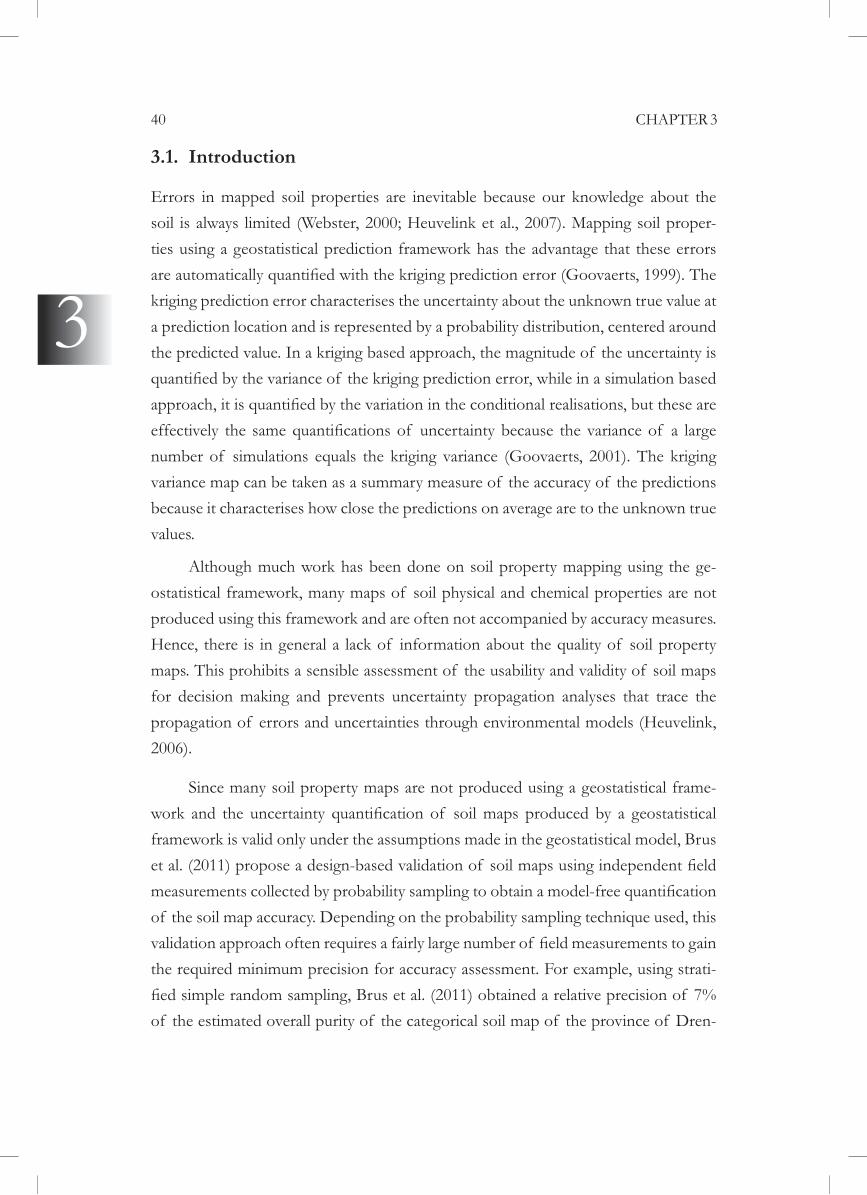
Errors in mapped soil properties are inevitable because our knowledge about the soil is always limited (Webster, 2000; Heuvelink et al., 2007). Mapping soil proper-ties using a geostatistical prediction framework has the advantage that these errors
kriging prediction error characterises the uncertainty about the unknown true value at a prediction location and is represented by a probability distribution, centered around the predicted value. In a kriging based approach, the magnitude of the uncertainty is
variance map can be taken as a summary measure of the accuracy of the predictions because it characterises how close the predictions on average are to the unknown true values.
Although much work has been done on soil property mapping using the ge-ostatistical framework, many maps of soil physical and chemical properties are not produced using this framework and are often not accompanied by accuracy measures.
maps. This prohibits a sensible assessment of the usability and validity of soil maps for decision making and prevents uncertainty propagation analyses that trace the propagation of errors and uncertainties through environmental models (Heuvelink, 2006).
Since many soil property maps are not produced using a geostatistical frame-
framework is valid only under the assumptions made in the geostatistical model, Brus
-
of the estimated overall purity of the categorical soil map of the province of Dren-

SPATIAL UNCERTAINTY QUANTIFICATION 41
3
the, The Netherlands with 150 validation observations. Malone et al. (2011) combine model-based and design-based approaches to introduce two new measures of the
-
Moreover, independent validation only provides summary measures of the map ac-curacy and does not yield a full spatial-probabilistic description of the uncertainty as
-
soil maps based on their experience and knowledge. In such cases, when independent
2012; Perera et al., 2012a). Experts, and the knowledge they provide, can be valuable
2001; Krueger et al., 2012).
In this chapter, we aimed at applying an existing statistical expert elicitation
Anglian Chalk area of The United Kingdom. The SWFC map is part of the National Soil Map of England and Wales (NATMAP). The SWFC map can be prone to un-certainty due to measurement and mapping errors of the covariate data and errors in the pedotransfer function used to create the map (Minasny et al., 1999; McBratney et al., 2002; Minasny and McBratney, 2002). The SWFC map is used as one of the main inputs in a chain of models that predict regional future crop yield for the East Anglia Chalk area (UncertWeb, 2010). The uncertainty about the SWFC can lead to uncertainty in crop yield and hence, uncertainty propagation can cause bias and lack of precision in the yield prediction outcomes.
The results from this chapter are meant to serve as a demonstration of how -
erties. Also, the presented work is meant to show the use of the elicitation protocol
42 CHAPTER 3
3
and web-based tool for expert elicitation of the variogram as proposed in Chapter 2. In Section 3.2, we elaborate on the materials and methods used in this work. Section 3.3 presents the results of the case study. In Section 3.4, we discuss the results, draw conclusions and give recommendations for future research.
3.2. Materials and Methods
3.2.1. Description of the study area
The study area is located in East Anglia in the southeast of The United Kingdom (Fig. 3.1). The mainly arable region was formed on a narrow continuation of the chalk ridge that runs from southwest to northeast across southern England. The region is about 839 km2 in size, spanning about 69 km along its longest dimension; its width ranges from about 10 km to 20 km. The altitude of the region gradually increases from about 0 meters in the northeast to about 167 meters above sea level in the south-
7, the East Anglia region is drier than other regions in The United Kingdom: it has a low annual rainfall (less than 700 mm per year) with much more even distribution of rainfall throughout the year than most other parts of The United Kingdom. The mean annual temperature is about 9-10ºC; the difference in temperature between winter and summer is about 10-15ºC. According to NATMAP - soil map of the East Anglia region, the main soil types over the study area are loam over chalk, sandy loam, deep clay and shallow silty over chalk.
In this study, the SWFC is the volumetric water content at 10kPa suction. The SWFC map for the East Anglian Chalk area (Fig. 3.2) is part of the NATMAP8. The NAT-MAP is a vector map with national coverage for England and Wales. It was produced
-dom. The map has a scale of 1:250,000.
The values of the SWFC map for the East Anglian Chalk area are expressed in a
are ‘representative’ for the dominant soil series associated with the polygons in the map. The values are computed by applying a pedo-transfer function that predicts the SWFC from basic soil properties (clay, silt, organic carbon and bulk density) using a multiple linear regression derived from the soil survey of England and Wales (Hall et al., 1977).
7 http://www.metoffice.gov.uk8 http://www.landis.org.uk.

SPATIAL UNCERTAINTY QUANTIFICATION 43
3
The values of the basic soil properties per soil series used in the regression are based on observations taken across England and Wales of which the mean values per soil series of these properties are computed and assigned to corresponding polygons on the map.
Figure 3.1: East Anglian Chalk area
In addition, maps of soil type, land cover, texture, bulk density, geology, eleva-tion and climatic information for the study area were used as ancillary information and provided to experts. These maps were also extracted from the NATMAP vector data.
3.2.3. Design of expert elicitation procedure
because in reality, the exact value of the error at any location in the study area is un-
Heuvelink et al., 2007). In order to facilitate experts to characterise this full spatial probability distribution, we used a formal expert elicitation framework following the

44 CHAPTER 3
3
Particularly, we used the web-based tool that was designed for expert elicitation for the variogram (Chapter 2). By using this tool, we implicitly assumed that the random function model of the error is either normally or log-normally distributed, and is sec-ond-order stationary. We now describe the steps of the framework.
Step 1: Characterisation of uncertainty
map at any location in the study area: ˆZ X Xs s s , where Z is the error value
at a location s D, D is the study area, X is the SWFC value provided by the map and X is the true value of the SWFC. The true value is the SWFC of a core taken at 25 cm depth. Experts were asked to take all sources of error that cause the map value to differ from the true value into account.
SPATIAL UNCERTAINTY QUANTIFICATION 45
3
As already mentioned, the error was assumed to have either a normal or log-nor-mal distribution. Further, we assumed that the error is second-order stationary and isotropic. This means that its spatial mean and standard deviation are location-inde-pendent and that the spatial correlation of the error at two locations only depends
h
correlation is characterised by the variogram.
The probabilistic model of the error {Z(s), s Z(s) = + (s), where Z(s) is a random variable that represents the error at location s, is the spatial mean error that depicts the bias in the SWFC map, the stochastic error is a sec-ond-order stationary and isotropic random function with zero mean and variogram function: (h) = Z(h) s+h) – Z(h))2] (Goovaerts, 1997), where stands for the variogram.
Step 2: Selection of experts
We selected experts through a two-step procedure. First, we nominated a list of ex-perts. Based on this list, we studied their CVs to have a better understanding of
peer-reviewed papers in soil science, particularly in agricultural hydrology. Experience was derived from the time they started their research in soil science. Motivation was
this way, we selected ten experts from The United Kingdom and The Netherlands with a high level of expertise, at least ten year experience in soil science with a good level of motivation and who are familiar with the study area. All selected experts have
-lected experts, we sent them by email an invitation letter for the elicitation exercise.
Kingdom were willing to participate in the full elicitation procedure. The others could
to achieve robust results (Knol et al., 2010).
Step 3: Design of the elicitation protocol
In this step, we adopted the web-based protocol for expert elicitation of the vario-

46 CHAPTER 3
3
gram (Chapter 2) which allows to elicit from experts the mpdf and the variogram to form the full spatial distribution of the spatial random error under the assumptions of a normal and log-normal distribution. There are two main rounds in the elicita-tion protocol. Round 1 is the elicitation of the mpdf and Round 2 is the elicitation of the variogram (Fig. 2.1). By using the web-based tool, the tasks in Step 2-Scope and format of the elicitation, Step 5-Preparation of the elicitation session and Step 6-Elicitation of expert judgements in Knol et al. (2010) were incorporated into this step. Implementing this step is the most laborious task among all steps.
After experts were given usernames and passwords, they could access the tool at: http://www.variogramelicitation.org. We designed an introduction page that provid-ed the experts with a detailed description of the study area, information and map of the SWFC together with maps of all auxiliary variables as described in Section 3.2.2. The introduction was provided to familiarise the experts with the context and pur-pose of the case study.
---
outcomes from the elicitation were to be presented in a research paper aiming at stu-dents, experts, decision makers and scientists in crop yield modelling and soil science.
experts in giving their judgements.
two weeks for the second round. For Round 1, because there were holidays in be-tween, the time lasted from 20th
to the experts until 6th
from 23rd of January, 2012 to 5th of February, 2012. We recommended that the actual
The web-based tool provided a mechanism for minimising bias in experts’ judge-

SPATIAL UNCERTAINTY QUANTIFICATION 47
3
pooling) for pooling multiple experts’ judgements.
The experts were contacted by email to start each of the elicitation rounds and
issues during the elicitation procedure.
Step 4: Evaluation and report of results
exercise, besides communicating with the experts during the elicitation session, we
covered two main aspects: the practicality of the elicitation exercise and the experts’ -
imum of ten minutes for each expert to complete.
Documentation of the elicitation procedure and presentation of the results are accomplished in this paper. The results are presented graphically and in the form of summary tables. Judgements by individual expert are reported anonymously.
3.3. Results
-cause we anonymously report judgements from each expert, we encode the six ex-
The variogram lags are encoded as Lj of which the index j = 1, ..., 7 numbers the lags from the shortest to the longest lag. Recall that Z denotes the isotropic second-or-der stationary spatial random error in percentages. The results of the two elicitation rounds are presented in turn.
48 CHAPTER 3
3
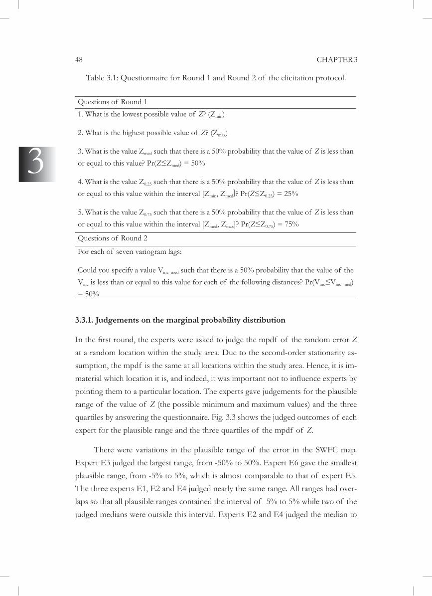
Table 3.1: Questionnaire for Round 1 and Round 2 of the elicitation protocol.
Questions of Round 11. What is the lowest possible value of Z? (Zmin)
2. What is the highest possible value of Z? (Zmax)
3. What is the value Zmed Z is less than Z med
4. What is the value Z0.25 Z is less than
min, Zmed]? Pr(Z 0.25
5. What is the value Z0.75 Z is less than
med, Zmax]? Pr(Z 0.75
Questions of Round 2
For each of seven variogram lags:
Could you specify a value Vinc_med
Vinc inc inc_med)
3.3.1. Judgements on the marginal probability distribution
Z at a random location within the study area. Due to the second-order stationarity as-sumption, the mpdf is the same at all locations within the study area. Hence, it is im-
pointing them to a particular location. The experts gave judgements for the plausible range of the value of Z (the possible minimum and maximum values) and the three
Z.
There were variations in the plausible range of the error in the SWFC map.
The three experts E1, E2 and E4 judged nearly the same range. All ranges had over-
judged medians were outside this interval. Experts E2 and E4 judged the median to

SPATIAL UNCERTAINTY QUANTIFICATION 49
3
values of all experts resulted in a (more or less) symmetric distribution around the
density function to the expert’s judged values are shown in Fig. 3.4.
Table 3.2: Information about experts participating in the study
Expert Title ExpertiseE1 - a - Land surface modelling,
soil physical, hydro-mete-orological and plant-phys-iological measurement methods
E2 Department of Geog-raphy & Environmental Science, University of Reading
Professor in Soil Science Soil science, Pedometrics
E3 Computer Science, As-ton University
Reader in Computer Science
Environmental Statistics, Geo-Informatics
E4 Department of Geog-raphy, Brigham Young University
Associate Lecture Soil Science
E5 Rothamsted Research Lawes Trust Senior Fellow
Soil science, Pedometrics
E6 Soil Physics and Land Use Team, Alterra, Wa-geningen University
Senior Researcher Soil Sciences, Soil Physics, Land Evaluation
aE1 wishes the information to remain anonymous.

50 CHAPTER 3
3
Figure 3.3: Judged values from six experts for the minimum, maximum and the
chosen location in the study area
Figure 3.4: Fitted marginal probability density functions to individual expert’ judgements and to the pooled opinion

SPATIAL UNCERTAINTY QUANTIFICATION 51
3
-
probability density functions to experts’ judgements. Experts E2 and E4 judged that
-ted standard deviation measures the absolute degree of variation in the random error.
smaller than those of all other experts. This is also depicted in Fig. 3.4 by the two narrow probability density graphs for experts E5 and E6.
As also shown in Fig. 3.4, the pooled mpdf that is a probabilistic average of all
experts’ judgements
Expert
E1 0.0 18.2E2 8.0 15.8E3 0.0 14.8E4 8.0 12.9E5 0.0 2.2E6 0.0 3.1
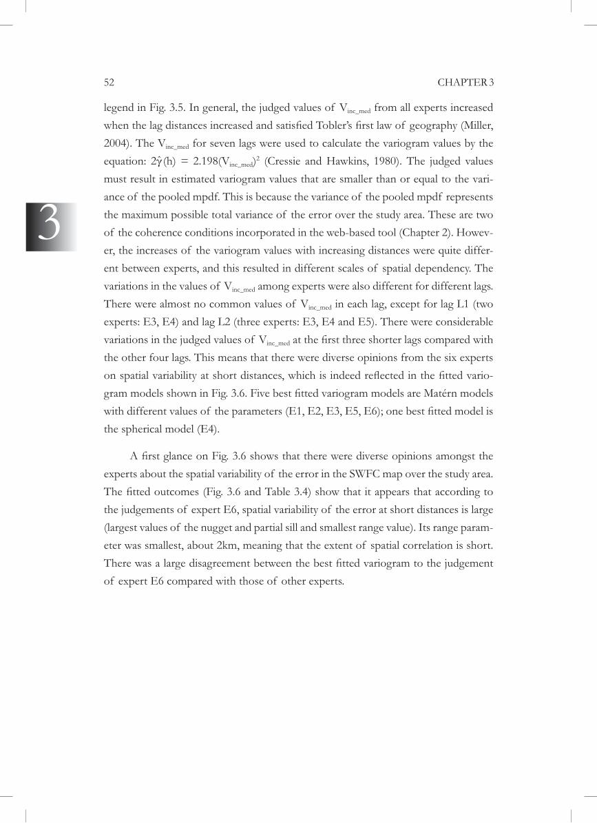
3.3.2. Judgements on the variogram
Variogram elicitation was started by eliciting the median of the absolute values of
inc Z(s) Z(sdistances h (Chapter 2). We denote this median by Vinc_med. The seven lags where the values of Vinc_med were elicited were estimated based on the extent of the study area. The seven lags Lj range from 0.5km to 50km and are shown on the bottom-right
52 CHAPTER 3
3
legend in Fig. 3.5. In general, the judged values of Vinc_med from all experts increased
2004). The Vinc_med for seven lags were used to calculate the variogram values by the ˆ (h) = 2.198(Vinc_med)2 (Cressie and Hawkins, 1980). The judged values
-ance of the pooled mpdf. This is because the variance of the pooled mpdf represents the maximum possible total variance of the error over the study area. These are two of the coherence conditions incorporated in the web-based tool (Chapter 2). Howev-
-ent between experts, and this resulted in different scales of spatial dependency. The variations in the values of Vinc_med among experts were also different for different lags. There were almost no common values of Vinc_med in each lag, except for lag L1 (two experts: E3, E4) and lag L2 (three experts: E3, E4 and E5). There were considerable variations in the judged values of Vinc_med
the other four lags. This means that there were diverse opinions from the six experts -
the spherical model (E4).
experts about the spatial variability of the error in the SWFC map over the study area.
the judgements of expert E6, spatial variability of the error at short distances is large (largest values of the nugget and partial sill and smallest range value). Its range param-eter was smallest, about 2km, meaning that the extent of spatial correlation is short.
of expert E6 compared with those of other experts.

SPATIAL UNCERTAINTY QUANTIFICATION 53
3
inc_med) at seven spatial lags from six experts

54 CHAPTER 3
3
The variogram models of experts E1, E2 and E5 depict almost the same behav-iour at short distances: strong spatial correlation resulting in smooth variation (larger values of the kappa parameters of the Matérn models and smaller nugget effect). The range parameter of the model of expert E5 (7.5 km) and that of expert E2 (10 km) were shorter than that of expert E1 (20 km). This means that according to experts
gradual decrease of spatial correlation with increasing distance. The opinions of ex-
models to their judgements were also different among each other, the behaviours of
those of the other experts. This group of opinion seemed to be ‘moderate’, while the
expert E4 was the only spherical model that has a large range, large partial sill and also a large nugget. This model resulted in a combination of a noisy signal and gradually changing values over distances.
Table 3.4: Fitted variogram models to six experts’ judgements and their parameters.
Expert Model ParametersRange (meter) 2) 2) Kappa
E1 Matérn 19,623 0.34 68.88 1.1E2 Matérn 10,352 0.004 44.55 1.7E3 Matérn 6,918 0.73 27.92 0.4E4 Spherical 35,368 4.81 59.28 -E5 Matérn 7,575 0.09 37.47 2.0E6 Matérn 2,164 6.16 66.22 0.6
-iogram values that were the average values of all experts’ judgements for the sev-en lags (Chapter 2). The pooled variogram model is the Matérn model with pa-
2 2, range = 25,400 meters, kappa = 0.4. A set of simulated maps of the error based on the pooled mpdf
-an simulation (Fig. 3.7). Fig. 3.8 shows the simulated SWFC maps that were gen-

SPATIAL UNCERTAINTY QUANTIFICATION 55
3
erated by adding each of the simulated error maps to the SWFC map (i.e. Fig. 3.2).
3.3.3. Feedback from experts on the elicitation exercise
The feedback from the experts about the elicitation exercise concerned two aspects: feedback on the experts’ performances and on the practicality of the elicitation ex-
(see Appendix 3.A) that they received.
capacity for the East Anglian Chalk area

56 CHAPTER 3
3
Anglian Chalk area
SPATIAL UNCERTAINTY QUANTIFICATION 57
3
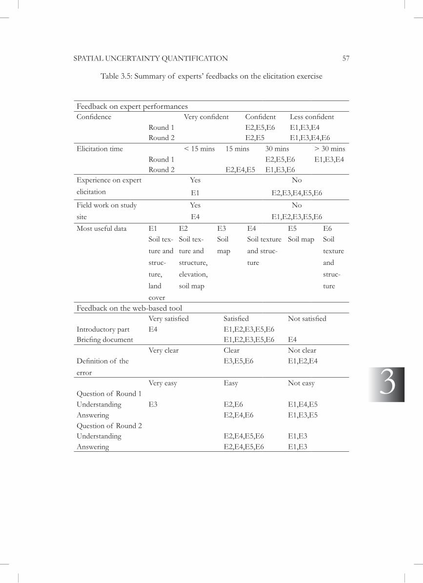
Table 3.5: Summary of experts’ feedbacks on the elicitation exercise
Feedback on expert performances
Round 1 E2,E5,E6 E1,E3,E4Round 2 E2,E5 E1,E3,E4,E6
Elicitation time < 15 mins 15 mins 30 minsRound 1 E2,E5,E6 E1,E3,E4Round 2 E2,E4,E5 E1,E3,E6
Experience on expert elicitation
Yes No
E1 E2,E3,E4,E5,E6Field work on study site
Yes NoE4 E1,E2,E3,E5,E6
Most useful data E1 E2 E3 E4 E5 E6Soil tex-ture and struc-ture, land cover
Soil tex-ture and structure, elevation, soil map
Soil map
Soil texture and struc-ture
Soil map Soil texture and struc-ture
Feedback on the web-based tool
Introductory part E4 E1,E2,E3,E5,E6E1,E2,E3,E5,E6 E4
Very clear Clear Not clear
errorE3,E5,E6 E1,E2,E4
Very easy Easy Not easyQuestion of Round 1Understanding E3 E2,E6 E1,E4,E5Answering E2,E4,E6 E1,E3,E5Question of Round 2Understanding E2,E4,E5,E6 E1,E3Answering E2,E4,E5,E6 E1,E3

58 CHAPTER 3
3 Round 2, the time they spent on this round was less than that for Round 1. All experts spent at least thirty minutes on Round 1. In Round 2, the two experts who expressed
time of 30 minutes while the rest spent the maximum of 30 minutes. This contrasts with our expectation that experts would spend more time carefully examining the
Continuing on the performance of the experts, only one expert had previous
work in the study area, although all were familiar with the soils in this region. We were interested in which information was most important for the experts to base their judgements on. Four experts found the information about soil texture and structure of the study area most useful. The other two experts found the soil map most useful.
the tool. During the elicitation procedure, there was no complaint about the function--
tory part, although one expert felt somehow distracted by the interesting background
-eral experts initially interpreted the error as the absolute error, meaning that it could
-

SPATIAL UNCERTAINTY QUANTIFICATION 59
3
3.4. Discussion and Conclusions
In this section, we discuss the results of the expert elicitation process, especially their robustness and the possibility of bias. Robustness here means how closely the six experts’ opinions represent the total expert community’s. We will also discuss the practicality of the web-based tool and facilitating expert elicitation using the web-based tool.
The spatial probability distribution of the error in the SWFC map has a nor-
that the SWFC map was overall underestimated for all soil types (or at every location).
the systematic error is smaller than the random error. On average at every location
To elicit the uncertainty of the SWFC map, we assumed that the spatial error
-sumed in geostatistics, but it is important to verify that the resulting model is a plau-sible description of reality. In our case, we assumed that the error in the SWFC has constant mean and variance, while it may be more realistic to relax this assumption and let it vary with soil type (e.g., larger uncertainty in stony soils). This could be a topic for follow-up research.
both the mpdf and the variogram. Unweighted averaging is simplistic but pragmatic -
ods (Clemen and Winkler, 1999; O’Hagan et al., 2006; French, 2011). Alternatively, weighted pooling can be used to give some experts larger weights than others. The
60 CHAPTER 3
3
weights can be interpreted in a variety of ways (Genest and McConway, 1990), e.g.,
of the informativeness of experts’ judgements and the experts’ performance (Cooke, 1991), etc. The weights can be assigned to experts by the analysts or the decision maker (French, 2011) or the experts can weigh each other and/or choose their own weights (i.e. self-assigned weights) (DeGroot, 1974; Genest and McConway, 1990).
experts and in which conditions using weighted average truly improves results com-pared to unweighted average (O’Hagan et al., 2006; Clemen, 2008). Therefore, we
The pooled outcomes can be interpreted as the average knowledge of six rep-
investigated case. Based on the recommendations from several publications that serve as guidelines to design and conduct a statistical expert elicitation, six experts should be enough to obtain robust results when considering the trade-off between expenses and informative gain (Meyer and Booker, 2001; Hora, 2004; Knol et al., 2010). We
soil properties of the study area. This makes the elicited results well representative for (diverse) opinions on the error of the SWFC map. Concerning the reliability of
in Round 2. We conclude that the elicited outcomes encapsulate the current knowl-edge of multiple experts of the error in the SWFC map for the East Anglian Chalk
The elicitation method we used is a variation of the Delphi method (Ayyub, 2001) where the experts’ judgements are anonymously and independently elicited. By examining the elicited outcomes from every expert, we see that the experts’ judge-ments for both the mpdf and the variogram seem to be clustered. The cluster of the judgements might indicate true consensus in a subgroup of experts about the error in the SWFC map. However, it can also indicate a correlation or dependence in experts’
The striking difference in judged values from Round 1 is that between the nonzero (E2 and E4) and zero median (E1, E3, E5 and E6) of the mpdf. Assuming that E2

SPATIAL UNCERTAINTY QUANTIFICATION 61
3
and E4 are completely dependent, one of the expert judgements would be eliminated from the pooling, then the positive bias would reduce. But, if experts in the second subgroup are completely dependent, only one opinion from the second subgroup can contribute to the pooling, in this case the positive bias increases. It would be inter-esting to examine the dependence in expert judgements. However, the feedback on experts’ performances (Table 3.5) and information about experts given in Table 3.2
is beyond the scope of this study. Moreover, in the context of web-based elicitation, detecting the occurrence of cognitive and motivational biases in the expert judging
-mances of the experts while giving judgements could not be observed.
Initially, the outcomes from Round 1 were systematically biased due to misin-
was elicited). Thereby, all experts redid the elicitation task for Round 1. This misin-terpretation might have been avoided by doing a pre-elicitation training (Knol et al., 2010); but, we did not include it in our four steps (Section 3.2.3). Moreover, although the elicitation session was prepared according to a formalised elicitation protocol,
experts prior to the elicitation exercise. These documents should ideally have been accessible to the experts at least two weeks in advance (Ayyub, 2001). The lack of a
some experts were familiar with giving probabilistic judgements, other experts found
probabilistic judgements prior to their involvement in the elicitation exercise (Hog-
familiarize experts to the elicitation exercise and giving probabilistic judgements and -
text of web-based statistical expert elicitation.
We can conclude from the case study that the web-based tool, which provides a uniform procedure to characterise the spatial probability distribution of uncertain variables from expert knowledge, functioned well. With the developed elicitation pro-
maps from expert knowledge. Simulated SWFC maps of the study site such as shown
62 CHAPTER 3
3
in Fig. 3.8 can be used to investigate the propagation of uncertainty from the SWFC map to the output of the regional crop yield model. This study also showed that
errors in) soil properties. This can overcome the limitations of using an average var-
lessons from our experiences of facilitating an elicitation exercise with a web-based tool:
1. The facilitators play a crucial role in the success of the elicitation exercise, also for the web-based elicitation methods where a self-elicitation process is expected.
2. Motivation is a very important criterion when choosing experts for the success of the elicitation exercise and reliability of the elicited outcomes.
3. Differences in experts’ opinions are legitimate (Morgan and Henrion, 1990); but reliable elicitation protocols are those that do not exaggerate these inherent differences.
4. To determine whether experts’ judgements are dependent, an extensive investi-
Booker, 2001).
-tively ascertain the generalisation of the elicitation results.
6. Computer tools are uniform, supportive and reusable mechanisms for eliciting expert knowledge, but they have the disadvantage compared to physical expert elici-tation meetings that experts’ performances cannot be monitored for the possibility of bias occurrence.
7. Precision in elicited outcomes from multiple experts might indicate a poor elic-itation protocol, while imprecision does not necessarily represent inaccuracy in ex-perts’ knowledge.
This study showed that statistical expert elicitation is a promising method to characterise spatial uncertainty of soil property maps using expert knowledge when data-based validation methods are not affordable or feasible. The value of expert

SPATIAL UNCERTAINTY QUANTIFICATION 63
3
knowledge in soil science was acknowledged as a valuable informative prior, especially when there are no alternative useful sources of information (Stein, 1994). Exploring, developing and applying reliable methods to extract knowledge from experts, e.g. using statistical expert elicitation for the variogram elicitation as done in this study, should be stimulated among soil scientists to effectively and reliably extract informa-tion from experts in soil research.
Appendix 3.A. Questionnaire for elicitation exercise evaluation
Dear Expert,
when it is ready to be published).
Thank you very much for your contribution to the elicitation exercise.
The elicitation team.

64 CHAPTER 3
3 error in the mapped soil water content?
Information Your choice
Soil texture and structure
Temperature
Soil map
Land cover
Annual precipitation
Geology map
Elevation map
Please specify any others:
capacity clear to you?
Clearness Your choice
Very clear
Clear
Not clear

SPATIAL UNCERTAINTY QUANTIFICATION 65
3
Easiness Round 1 Round 2Very easy
Easy
Not easy
Easiness Round 1 Round 2Very easy
Easy
Not easy
capacity?
Yes
No
8. How much time did you spend for each round of the elicitation exercise?
Time Round 1 Round 2Less than 15 minutes
15 minutes
30 minutes
More than 30 minutes
9. Have you ever participated in an elicitation exercise before?
Yes
No

66 CHAPTER 3
3
10. Do you have other comments on the elicitation exercise?
Chapter 4
Bayesian area-to-point kriging using expert knowledge as informative priors
Based on: Truong, P.N., Heuvelink, G.B.M., Pebesma, E., 2014. International Journal of Applied Earth Observation and Geoinformation 30, 128-138.

68 CHAPTER 4
4
4.1. Introduction
Spatial disaggregation (downscaling) is becoming more important in a world where the demand for data transformation from global to local scales is rapidly increasing.
spatial climate attributes (e.g. precipitation, air temperature or atmospheric vapour) at
using global climate models. Here, spatial resolution or pixel size stands for the spatial support, i.e. the geometrical size, shape and spatial orientation of a spatial unit of an observation or a prediction. Changing the spatial support of a variable changes its statistical and spatial properties (Schabenberger and Gotway, 2005). This is the well-known change of support problem (Cressie, 1996; Gotway and Young, 2002; Schabenberger and Gotway, 2005).
Spatial support and change of support problem have been acknowledged as an important source of uncertainty in remote sensing analyses due to aggregation and zoning effects (Marceau and Hay, 1999; Dungan, 2006). Spatial disaggregation of remotely sensed imagery through interpolation shows an important application of geostatistics to remote sensing analysis (Van der Meer, 2012). Well-known geostatisti-
Area-to-point (ATP) kriging and multivariate ATP kriging (Atkinson, 2013 ).
In this study, we focused on ATP kriging (Kyriakidis, 2004) for spatial disaggre--
ing and makes predictions of an attribute at point support (PoS) from block support
the condition that the arithmetic average of the predictions (and simulations) at all
of BSO are used as conditioning data (Goovaerts, 2008). Hence, to use ATP kriging, BSO must be (assumed to be) the arithmetic average of PoS data within the blocks.
Let z be the variable of interest that is assumed to be a realisation of a sec-ond-order stationary Gaussian random function Z and let z B = z1
BB
ii
i
d( ) ( )∈∫
s
s s be
the value of z at block support, where z(s) is the value of z at point location s and
iB is the area of a block B indexed by i. Because the arithmetic averaging is linear in
SPATIAL DISAGGREGATION 69
its argument, the random process at block support is also a Gaussian process.
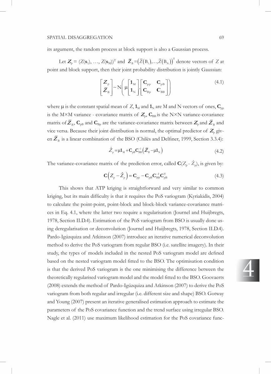
Let Zp = (Z(s1), …, Z(sM))T and denote vectors of Z at point and block support, then their joint probability distribution is jointly Gaussian:
(4.1)
where is the constant spatial mean of Z, 1M and 1N are M and N vectors of ones, Cpp is the M×M variance - covariance matrix of Zp, CBB is the N×N variance-covariance matrix of , CpB and CBp are the variance-covariance matrix between Zp and B and vice versa. Because their joint distribution is normal, the optimal predictor of Zp giv-
(4.2)
The variance-covariance matrix of the prediction error, called C(Zp - pZ ), is given by:
(4.3)
This shows that ATP kriging is straightforward and very similar to common
to calculate the point-point, point-block and block-block variance-covariance matri-
1978, Section II.D.4). Estimation of the PoS variogram from BSO is usually done us-ing deregularisation or deconvolution (Journel and Huijbregts, 1978, Section II.D.4).
method to derive the PoS variogram from regular BSO (i.e. satellite imagery). In their
is that the derived PoS variogram is the one minimising the difference between the
variogram from both regular and irregular (i.e. different size and shape) BSO. Gotway and Young (2007) present an iterative generalised estimation approach to estimate the parameters of the PoS covariance function and the trend surface using irregular BSO. Nagle et al. (2011) use maximum likelihood estimation for the PoS covariance func-
ΖΖ B 1 NT
= B , , BZ Z( ) ( )( )
ΖΖ
ΖΖp
B
M
N
pp pB
Bp BBN
⎡
⎣⎢⎢
⎤
⎦⎥⎥
⎡
⎣⎢⎢
⎤
⎦⎥⎥
⎡
⎣⎢⎢
⎤
⎦⎥⎥
⎛
⎝⎜⎜
⎞
⎠⎟⎟
μ1
1
C C
C, C
B
B
1p M pB BB B N1 C C 1ˆ
1ˆZ ZC C C C CTp p pp pB BB pB

70 CHAPTER 4
4
tion using BSO. Gelfand et al. (2001) address Bayesian estimation of PoS variogram parameters from BSO of a spatial-temporal process. Their study focuses on devel-oping objective Bayesian inference methods, where the priors of the PoS variogram model parameters are given as noninformative priors. This is one of few studies that addresses PoS variogram estimation from BSO using a Bayesian approach.
In all aforementioned methods for deriving the PoS variogram, the nugget com-ponent of the PoS variogram was dismissed and assumed to be zero. There was surprisingly little attention on resolving the issue of inferring the nugget parameter from BSO, despite the material impact of the nugget variance on the ATP prediction and associated uncertainty (Kyriakidis, 2004). From the performance assessment of the iterative numerical deconvolution method using irregular BSO, Goovaerts (2008) concludes that the behaviour at the origin of the PoS variogram model (i.e. the nug-get effect and within-block semivariance) could not be characterised with only BSO. Recently, Nagle et al. (2011) points out that the BSO retain little information to infer the nugget component of the PoS variogram and recommends using prior knowledge to overcome this problem.
The advantage of using a Bayesian approach is that the Bayesian estimator can
also the only formalised method to combine prior knowledge with BSO. However, extracting expert knowledge as informative priors is a delicate process in order to obtain reliable information. Much research has been done recently on using statis-tical expert elicitation to extract expert knowledge to use as informative priors for Bayesian statistical models, e.g. in Bayesian environmental and ecological modelling (Choy et al., 2009; Kuhnert et al., 2010; Kuhnert, 2011) and Bayesian geological mod-elling (Wood and Curtis, 2004). Formal statistical expert elicitation (Garthwaite et
from expert knowledge the probability distributions of the PoS variogram parame-ters to use as informative priors (Chapters 2 and 3). The statistical expert elicitation
the real elicitation task with experts to post-processing and using the statistical expert elicitation outcomes. There is increasing literature presenting detailed guidelines of developing and using statistical expert elicitation methods, e.g. Hahn (2006), Knol et

SPATIAL DISAGGREGATION 71
al. (2010), Kuhnert et al. (2010), O’Hagan (2012) to name a few. This promises to be a
component of the PoS variogram.
Our aim in this study was twofold. Firstly, we wanted to resolve the issue of poor estimation of the nugget effect from BSO by using a Bayesian approach that
propagation of PoS variogram parameters and ATP kriging model uncertainty to the disaggregated outcomes using Bayesian ATP conditional simulation. We illustrate the method with an example on disaggregating MODIS air temperature data measured
remainder of this paper has three main sections. Section 4.2 presents the statistical methods and a description of the example. Section 4.3 presents the main results of the study and a discussion. Section 4.4 provides the conclusions and recommenda-tions for further research.
4.2. Materials and methods
Figure 4.1 shows the three main steps of the method.
Figure 4.1: Three main steps of Bayesian area-to-point kriging method
4.2.1. Data
Spaceborne thermal imagery is becoming important in climate modelling, soil mois-ture assessment, irrigation management, etc. (Kuenzer et al., 2013a; Ha et al., 2013). Products of daily spaceborne thermal imagery often have lower spatial resolution (e.g., MODIS: 1 km to 5 km, NOAA-AVHRR: 1 km, Sentinel 3-ESA future mission:

72 CHAPTER 4
4
urban heat effect (Kuenzer et al., 2013b). For these reasons and for illustration pur-
product (MOD07_L2) as BSO of a continuous variable. The study area was the Gel-derland province, The Netherlands (Fig. 4.2). It is located in the east of The Nether-lands with a total area of 5,137 km2. The MOD07_L2 dataset (cloud-free, Collection 5) of August 1st, 2012 at 10:05 a.m. UT (i.e. 12 a.m. CEST) at 5 km resolution was obtained from LAADS Web - Level 1 and Atmosphere Archive and Distribution Sys-tem9
extracted and subset to the area of the Gelderland province (Fig. 4.3). The BSO of the study area had a mean of 21.6ºC and a standard deviation of 0.85ºC.
4.2.2. Statistical expert elicitation for prior distributions
to extract multiple expert knowledge for the prior distributions of the PoS variogram parameters.
parameters (i.e. sill, nugget, range and smoothness parameters) as the target variables of the elicitation task. The smoothness parameter of the Matérn variogram model
The Matérn variogram model p is given by:
p(h) = c0 + c11 ))(h/r) K
function of the second kind of order , c0 is the nugget variance, c1 is the partial sill variance, r is the range parameter, and is the smoothness parameter.
knowledge about the temperature variation within the Gelderland province. We also
researchers (two from Wageningen University and one from KNMI - Royal Nether-lands Meteorological Institute) were recruited into the online elicitation task lasting for two weeks from January 3rd, 2013 to January 17th, 2013.
9 http://ladsweb.nascom.nasa.gov/data/search.html.
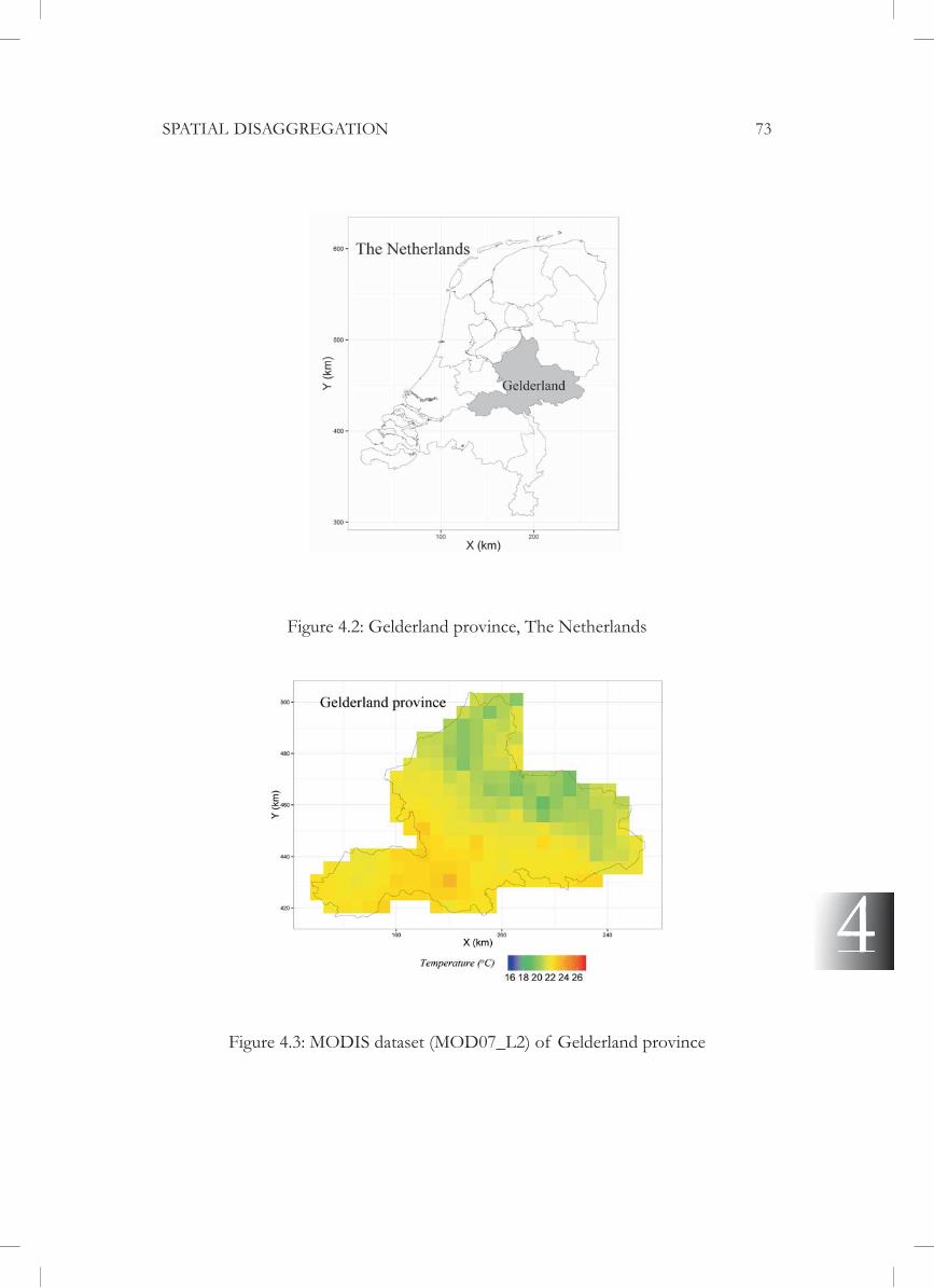
SPATIAL DISAGGREGATION 73
Figure 4.2: Gelderland province, The Netherlands
Figure 4.3: MODIS dataset (MOD07_L2) of Gelderland province

74 CHAPTER 4
4
Figure 4.4: Formal statistical expert elicitation procedure
study and all assumptions related to the dataset and the Matérn variogram model,
elicit the vairogram parameters, and (4) the common causes of biased judgements. Because the experts have expertise in geostatistics, there was no explanation provided
week in advance. They were informed of the possibility to gather all possible sources -
itation task.
Step 4: we set up the elicitation task where the experts were facilitated by the MATCH Uncertainty elicitation online tool10 (accessed 21/03/2013) to independent-ly and individually judge the probability distributions of the PoS Matérn variogram
10 http://optics.eee.nottingham.ac.uk/match/uncertainty.php

SPATIAL DISAGGREGATION 75
probability density function (pdf) of each parameter (available on the MATCH tool) and the variogram generated from the pdfs of the four parameters. A guideline of how to proceed with the elicitation task using the MATCH tool was given. The ex-perts were asked to spend time on self-training in giving probabilistic judgements with the MATCH tool. Thereby, we provided a week for the experts in total, of which only 45 minutes was recommended to complete the elicitation task for all four parameters.
(maximum, minimum, mean and standard deviation) of the pdfs that best conveyed the experts’ beliefs about the probability distributions of the parameters.
Three elicited pdfs from the three experts for each parameter were probabil-
1999; O’Hagan et al., 2006; French, 2011) to derive a single prior probability density
in all experts’ knowledge. These combined pdfs were used as informative priors in the Bayesian ATP estimator.
4.2.3. Bayesian ATP estimator using Markov Chain Monte Carlo
Assuming that the spatial random process characterising air temperature at PoS, called Z, over the study area is a Gaussian isotropic second-order stationary random pro-cess, it is fully characterised by the mean and variogram: Zp ~ N( , p). The variogram
p = p(h, ) is a function of the Euclidean distance h and the vector of four pa-rameters of the Matérn variogram. Block averages: B ~ N( , ) have the same spa-tial mean (Gotway and Young, 2002) but a different spatial structure. is the block support variogram and a function of the distance h and the vector of parameters .
In Bayesian estimation, the joint posterior distribution of and is related to
p( ) ( )L( ) (4.5)
where p( ) is the joint posterior distribution, ( ) is the joint prior distribution and L( ) is the likelihood. The joint prior distribtion of -ate kernel density to the pooled pdfs of all four variogram parameters.

76 CHAPTER 4
4
The likelihood of and conditioning on BSO is given by:
Approximately numerical calculation of each item of CBB is:
where the i, j index the BSO (i, j = 1, …, N), the k and l index the discretised points
within blocks and K is the number of discretisation points per block. Blocks were
The ‘Metropolis within Gibbs’ or hybrid MCMC algorithm (Chib and Green-berg, 1995; Robert and Casella, 1999, Chapters 6 and 7; Albert, 2009, Chapter 6) that simultaneously uses both Gibbs sampling steps and Metropolis-Hastings steps
sampler to iteratively and alternatingly sample from its full distribution conditional on and sample from its full distribution conditional on . To simulate a set of from the full conditional distribution on , the Metropolis-Hastings algorithm was used because their joint conditional distribution cannot be sampled directly. The same approach was used for . We used Geweke’s convergence diagnostic test (Geweke, 1992) to test the convergence of the MCMC chains to stationary distributions.
The hybrid MCMC was implemented in R (R Core Team, 2013), gstat package (Pebesma, 2004) for implementing ATP kriging, and the geweke.plot function of the CODA package for convergence diagnostics (Plummer et al., 2006). These computa-tions resulted in successive sets of and that were thinned to obtain a reasonably independent set to use as input to ATP conditional simulation (Section 4.2.4).
4.2.4. ATP conditional simulation
ATP conditional simulation enables to generate realisations of Z at PoS conditional on BSO . We applied the approach of stochastic conditional simulation by gener-
kriging of the differences between the BSO and simulated block arithmetic averages Zpcs as the
L =2 expB BB1
2 B NT
BB1
B NN
21
2μ π μ μ,θθ Z Z Z( ) −( ) −( ) −( )⎡⎣⎢
⎤⎦⎥{ }− − −C 1 C 1
C
s s
BB
cK
2K K-1 1 0
1K
i, jc c i = j1
2
[ ] =+ ( ) + − −( )( )
( )
( )>=∑∑ γp k
k
K
k
K
ll1
,
cc i=1
1 01
+ − −( )( ) ≠
⎧
⎨⎪⎪
⎩⎪⎪ ∑∑
=
c p k
K
k
K
γ s sll
, j
B

SPATIAL DISAGGREGATION 77
ATP conditional simulation at PoS, it can be shown that:
(4.6)
where Zps is the PoS unconditional simulation and pkZ is ATP simple kriging of the difference between BSO and the simulated block arithmetic average Bs.
Practical implementation of this approach comprised four steps:
Step 1. Unconditional simulation at PoS prediction locations: unconditional
grid for each set of PoS variogram parameters derived from the Bayesian ATP esti-mation (Section 4.2.3).
Step 2. Aggregating each PoS unconditional simulation to block support to obtain Bs and calculating the difference:ΔΖΖ ΖΖ ΖΖ= B − Bs .
Step 3. ATP simple kriging of ΔΖΖ at PoS prediction locations to obtain pkZ
Step 4. Summing Zps and pkZZpcs.
All four steps were implemented in R (R Core Team, 2013).
4.3. Results and Discussion
4.3.1. Informative priors from multiple expert knowledge
We anonymously report the elicitation outcomes from the three experts, named Ex-pert 1, Expert 2 and Expert 3. Figs. 4.5 - 4.8 show the pdfs of the four parameters of the PoS Matérn variogram model that, according to the experts, best convey their opinion about the probability distributions of these parameters. Tables 4.1 provides summary statistics of these pdfs.
pcs ps pkˆ= +Z Z Z

78 CHAPTER 4
4Figure 4.5: Probability density functions of partial sill parameter from three experts
Figure 4.6: Probability density function of nugget parameter from three experts and

SPATIAL DISAGGREGATION 79
Figure 4.7: Probability density function of range parameter from three experts and
15
Figure 4.8: Probability density function of kappa parameter from three experts and

80 CHAPTER 4
4
Table 4.1: Elicited outcomes from experts
Parameters Pdf Minimum Maximum Mean Standard deviation
Expert 1Partial sill (°C2) Log-normal 9.0 16.0 2.5 0.17Nugget (°C2) Log-normal 0.5 9.0 1.5 0.59Range (km) Normal 3.0 10.0 6.5 2.17Kappa Log-normal 1.0 10.0 1.6 0.53Expert 2Partial sill (°C2) Normal 1.0 10.0 4.7 2.20Nugget (°C2) Normal 0.0 3.0 1.2 0.44Range (km) Normal 25.0 151.0 63.0 29.84Kappa Normal 3.0 5.0 4.0 0.44Expert 3Partial sill (°C2) Scaled-beta 0.0 4.0 4.7 3.14Nugget (°C2) Normal 0.0 1.0 0.3 0.14Range (km) Scaled-beta 0.0 80.0 2.7 4.69Kappa Log-normal 0.4 4.0 0.4 0.24
-ty of the parameters of the PoS variogram. In particular, there was little agreement among the experts about the values of the sill and the nugget parameters. Their pdfs have modes located at different values. The different widths of the pdfs indicat-ed different level of experts’ uncertainty about these parameters. The variograms in Fig. 4.9 show a better agreement among the experts for the effective range (i.e. the
is not apparent from Figs. 4.7 and 4.8 for the range and smoothness parameters. The reason is that there is a correlation between the smoothness parameter and the range parameter: a large range parameter corresponds to a small smoothness parameter and vice versa, which when combined, results in similar variograms. Although the effective ranges are similar, the variograms from Experts 1 and 2 approach the origin differently with different combinations of smoothness and range. Compared to the extent of the study area, the judgements of Expert 2 resulted in a very smooth spatial process, while those of Expert 1 resulted in a much more rough spatial process.

SPATIAL DISAGGREGATION 81
Figure 4.9: Experts’ prior variograms
The elicitation procedure had the form of a Delphi elicitation process for mul-tiple experts (Kuhnert et al., 2010), of which the feedback of the pdfs and the vari-ogram provided a mechanism for calibrating experts’ judgements regarding the best expression of their opinions. The difference from the traditional Delphi method is that the outcomes from each expert were not given as feedback to other experts. This kept maximum diversity in expert opinions. To validate the experts’ judgements, we had measured data from only three KNMI meteorological stations located across the Gelderland province. The data were too few to make an accurate estimation of the PoS variogram for validation. Using KNMI station data of the whole of The Netherlands, the PoS variogram derived from these data (see Salet, 2009) agreed well
terms of spatial and temporal extent. In fact, we consulted the experts because of
Gelderland province.
Although Expert 1 had a remarkably different opinion about the sill and nugget

82 CHAPTER 4
4
because of the reasoning behind the judgements of this expert. Disagreements in experts’ judgements that result from differences in experts’ perception or in weighing and combining various sources of knowledge and information can bring more infor-mation but can also imply large uncertainty in the current experts’ knowledge. Even though the experts have expertise in geostatistics, prior knowledge elicitation of the
This can partly explain the large uncertainty and diversity in the experts’ judgments.
4.3.2. Bayesian ATP estimation of point support Matérn variogram model
distribution for was the joint distribution of the pooled pdf of all parameters (Sec-tion 4.3.1). The prior for was a wide, uninformative uniform distribution ranging between 10°C and 40°C. Trace plots in Fig. 4.10 show well-mixing outcomes with an acceptance rate of 0.5 for and 0.25 for that satisfy the recommended acceptance rate for one-dimensional and multi-dimensional parameters (Chib and Greenberg, 1995). Geweke’s diagnostic test results (Fig. 4.11) show that the MCMC chain con-verged using 30,000 runs. Because the main focus of this work is on the PoS vario-gram model’s parameters, there will be no more elaboration on .
The pdfs of the PoS variogram parameters were plotted together with their informative prior distributions in Figs. 4.12 and 4.13. The posterior distribution of the nugget parameter is almost the same as its prior distribution, except some erratic
BSO did not provide information to identify the nugget component of the PoS vari-
information. Even though, there was considerable uncertainty in the experts’ opin-ions about the nugget parameter, the elicited informative prior brought valuable in-formation to the Bayesian ATP estimator.

SPATIAL DISAGGREGATION 83
Figure 4.10: Trace plots for point support Matérn variogram model parameters and spatial mean
Figure 4.11: Results of Geweke’s convergence diagnostic test

84 CHAPTER 4
4Figure 4.12: Informative prior and posterior probability distribution of nugget
parameter
The posterior distributions of the other PoS variogram model parameters devi-ated largely from their priors and were indeed much narrower. This implies that esti-mates of the other parameters were strongly driven by BSO. Fig. 4.14 shows the pos-terior variograms that were generated by several random sets of the four parameters. The total sill of the posterior PoS variogram is much larger than the total variance of BSO (0.73°C2), which agrees with the fact that block support data are smoother and have smaller variance than point support data (Gotway and Young, 2002). The effec-tive range was about 50 km in average. Fig. 4.15 shows a negative correlation between the range and smoothness parameter and high positive correlation between the partial
sill and the range parameter.
4.3.3. ATP conditional simulations
Fig. 4.16 shows maps of the outcomes from 1,000 ATP conditional simulations with 1,000 inputs of PoS variogram parameters. These inputs were obtained from the MCMC chains by thinning every 30th iteration to obtain a reasonably uncorrelated set. The mean of the conditional simulations ranged from 18.8ºC to 24ºC. All sim-
maps of the 5th (lower limit) and 95th

SPATIAL DISAGGREGATION 85
PoS. The number of simulations was not enough to obtain a stable estimate of the variance of the ATP simulations. However, the variance of the ATP simulations was
of the joint posterior of the variogram parameters (Fig. 4.17). This shows that uncer-tainty about the PoS variogram parameters can make a substantial contribution to the uncertainty about the PoS values at prediction nodes.
Figure 4.13: Informative prior and posterior distributions of partial sill, range and smoothness parameters

86 CHAPTER 4
4Figure 4.14: Posterior point support variograms
Figure 4.15: Correlation between point support Matérn variogram model parameters

SPATIAL DISAGGREGATION 87
Figure 4.16: Bayesian ATP conditional simulation outcomes (°C)

88 CHAPTER 4
4
Figure 4.17: Standard deviation of ATP conditional simulations (top) and that of ATP Kriging with modal variogram (bottom) (°C)
4.4. Conclusions and Recommendations
ATP kriging provides a methodological solution to allow maximum use of available
it does not introduce new sources of information (Atkinson, 2013). In this study, we introduced a new source of information, i.e. by using expert knowledge via inform-ative priors of the PoS variogram parameters. By using the Bayesian ATP estimator, we have shown that the nugget of the PoS variogram cannot be estimated by only
-servations at PoS, expert knowledge is the best or perhaps only source of informa-

SPATIAL DISAGGREGATION 89
tion available about the nugget effect at PoS. For the other parameters, the posterior distributions are narrower than the priors because the BSO did provide real infor-mation, which also affected the correlations between these parameters. The example also showed that uncertainty about the PoS variogram parameters can substantially contribute to the overall ATP kriging prediction uncertainty.
The example illustrated that our proposed approach worked well, both in the-ory and practice. By this, we were able to derive an appropriate estimator of the PoS variogram parameters to perform spatial disaggregation with ATP kriging. It is worth mentioning that the prior knowledge derived by statistical expert elicitation in the form of probability distributions is a delicate task and to keep in mind that the elici-tation outcomes are always imprecise (O’Hagan and Oakley, 2004). In this study, we took the view that the best statistical expert elicitation task is the one that can elicit the true opinions of the experts. Although our direct elicitation approach for the PoS variogram parameters was structured and transparent, we noticed that it was a fairly
-stract to experts. Moreover, biases in expert opinion can directly distort the elicitation outcomes; this impact might be less when using indirect elicitation. We recommend that indirect elicitation approaches, such as those proposed in Chapter 2, should be explored and extended to derive the prior probability distribution of the PoS vario-gram parameters in future research. ATP conditional simulation was time-consum-ing because all BSO and already simulated nodes at PoS were used as conditioning data in ATP conditional simulation (i.e. we used global ATP conditional simuation). Implementing ATP conditional simulation with a local neighbourhood or using the circulant embedding method (Dietrich and Newsam, 1993) will help to speed up the simulation.


Chapter 5
Incorporating expert knowledge as obser-vations in mapping biological soil quality indicators with regression cokriging

92 CHAPTER 5
5
5.1. Introduction
Geostatistics furnishes a statistical tool - kriging - for spatial prediction at unobserved
has the smallest prediction error variance among all unbiased spatial interpolation methods (Armstrong, 1998, Chaper 7; Schabenberger and Gotway, 2005, Chapter 5). In geostatistics, reality is treated as if it were a realisation of a random process that is characterised by a probability distribution, which includes the spatial dependence structure (i.e. the variogram). The variogram is estimated from the observations using the methods-of-moments (Matheron, 1963; Cressie, 1985) or maximum likelihood
-servations are used both for modelling the spatial dependence and kriging.
Statistical inference of variogram parameters is problematic when there are few observations because the sampling variance is often large and little information about short distance spatial variation is available (Webster and Oliver, 2007, Section 6.1.2). Also, prediction by kriging with few observations typically results in large prediction error variances because of the low sampling density (Frogbrook, 1999). In short, us-ing few observations for kriging produces inaccurate maps. Unfortunately, in many practical cases, only few observations may be available for mapping because of, for instance, poorly accessible areas or laboriously and expensively measured variables. An alternative to collecting extra measurements of the target variable to improve mapping is using ancillary data and/or soft data that are more easily or more cheaply obtained. The ancillary data could be point observations of auxiliary variables that are spatially correlated with the variable of interest as used in cokriging (Goovaerts and Kerry, 2010) or spatially exhaustive covariate layers used in regression kriging or kriging with external drift (Goovaerts, 1997, Chapter 6; Hengl et al., 2007) while soft data are typically associated with the observations of the target variable that have (larger) measurement error. Such soft data could be measurements with a cheaper and less accurate instrument (e.g. Hamzehpour et al., 2013), but these could also be
-porated in kriging using cokriging and Bayesian kriging (Omre,1987; Goovaerts, 1997, Chapter 6).
There have been few studies that use expert knowledge as soft data to supple-
SPATIAL INTERPOLATION 93
5
guesses of plausible ranges of values in indicator cokriging, but without further inves-
guesses of the expected surface of a spatial process with uncertainty as prior infor-
expert judgements but does not provide a description of how expert judgements are obtained nor an evaluation of the use of expert knowledge for kriging. Lele and Das (2000) and Lele and Allen (2006) use expert knowledge as exact estimates of the
observations on the estimation of the spatial structure (i.e. the trend and the spatial correlation) is investigated, but the method used to extract expert judgements is not elaborated. These studies show the potential of using expert knowledge as supple-mentary data to direct measurements of the target spatial variable in mapping, but they lack a clear and formalised way to extract expert knowledge, and the important fact that expert judgements are uncertain is often ignored.
In this chapter, we propose to use expert knowledge as probabilistic soft data to augment direct measurements to map spatial variables by cokriging. To our knowl-edge, the use of expert knowledge in this way has not been investigated before. Prob-abilistic soft data are soft data recorded in the form of a probability distribution. We use soft data given by experts to improve variogram estimation and kriging. The rationale behind this is that expert knowledge can provide a valuable source of in-formation about spatial variability (Stein, 1994; Chapters 2 and 3). Statistical expert
a probabilistic form (Garthwaite et al., 2005; O’Hagan et al., 2006). However, data derived from expert knowledge cannot simply be treated as additional observations, and their different characteristics must be recognised in geostatistical inference and
-tors in a semi-natural grassland in The Netherlands.
During the last decades, biological soil indicators have been increasingly used not only to indicate soil threats such as soil degradation and contamination but also to indicate the ability of the soil to provide valuable ecosystem services such as the

94 CHAPTER 5
5
habitat forming for species rich natural ecosystems (Wall, 2004). Nematodes are the
index (SI) and enrichment index (EI). Nematodes occur mostly in high abundances and are positioned in the soil food web at all different trophic levels: herbivores, mi-crobivores, omnivores and predators (Yeates, 2003). Differences in life-history traits of nematode species form the basis of the SI and EI (Ferris et al., 2001). Nematodes can be grouped into (rapid growing) enrichment opportunists and general oppor-tunists and (slow growing) persisters. The ratio between enrichment opportunists and general opportunists is the EI, and the ratio between the persisters and general opportunists is the SI (Ferris et al., 2001). A high EI indicates high soil fertility, i.e.
to environmental stress or disturbance (de Goede et al., 1993; Ferris et al., 2001). Although the conceptual framework of these indices is well developed and current
expensive and time-consuming. Moreover, soil biological properties like nematode as-semblages may vary strongly over space (Ettema and Wardle, 2002). Therefore, the EI and SI are relevant variables for which the value of incorporating expert knowledge may be investigated.
Section 5.2 describes the geostatistical model used for incorporating expert knowledge in spatial inference and prediction. Section 5.3 presents the case study and
discussed in Section 5.4.
5.2. Methods
We consider the case where the variable of interest is modelled by a spatial Gaussian
that the measured data are error-free, while the expert data can be biased and im-precise and have different error variances that measure the expert uncertainty about
Z1 represent the
SPATIAL INTERPOLATION 95
5
measured data at n locations si, i = 1, …, n within a spatial domain D and let Z2 rep-resent the expert data at m locations sj, j = 1, …, m. Note that, in this study, the si are a subset of the sj
Z1(s) = F(s) 1+e1(s), where:
1 = { 1k -
cients, F ss
s( ) ( )
( )⎧⎨⎩
⎫⎬⎭
== 0, k = 0 , k = 1, , p
0
k
ff …
is a (p+1) vector of covariates at any location s
in D, and e1 denote the n×n variance-covariance matrix of the Z1 at the measurement locations by C11.
Z2(sj) = Z1(sj) + m (sj) + (sj e1(sj), where the zero-mean Gaussian random variables (sj) represent the random errors of the expert data. It is assumed that the (sj) are mutually independent and independent of e1(sj). The m (sj) represents the systematic error (bias) of the expert data, which is taken as a sum of a constant and a linear combination of the covariates, to capture
-iates on the target (dependent) variable. The term e1(sj) measures the conditional bias toward the mean (i.e. the smoothing effect of the expert judgements), with a
Z1 and Z2 have the same set of covariates because they model the same variable of interest. Substituting the model of Z1 in that of Z2 gives Z2(sj) = F(sj) 2 + e2(sj), where 2 = { 2k of unknown e2(s) = (s) + (1 )e1(s)~N(0,C22), with C22 a variance-covariance matrix derived from the covariance structures of e1 and . The
covariates: m (s) = F(s 2 1].
5.2.2. REML estimation
non-stationary spatial trend, REML estimates of covariance parameters of a Gauss-
compared to maximum likelihood estimation and the method-of-moments (Schaben-berger and Gotway, 2005, Section 5.5; Lark et al., 2006). Recall that the locations of expert data include the locations of the measured data. Because of this, the trend and

96 CHAPTER 5
5
Section 5.4; Wackernagel, 2003, Section 23).
Hence, we transform Z1 to Z1* = A1
Z1, where A1
removing the last p+1 rows of I F F F Fn 1 1T
1
1
1T−
−( )
F1 = F(si) is the n×(p+1) design matrix of Z1, In is the n×n identity matrix. Simi-larly, for Z2 A2 by removing the last p+1 rows of I F F F Fm
T 1 T−−
2 2 2 2( ) , Z2* =A2Z2 F2 = F(sj) is the
m×(p+1) design matrix and Im is the m×m identity matrix.
Because Z1 and Z2 are linearly transformed, and are also jointly normally distributed and both have zero mean due to the trend removal transformation. The likelihood is derived from the multivariate Gaussian probability density function:
, 21N 22* * * *T * 1 *1
21 2L expZ Z Z Z
The log-likelihood is:
(5.1)
where: N=n+m 2 p , ZZ
Z
A Z
A Z* 1
*
2*
1 1
2 2
= =⎡
⎣⎢
⎤
⎦⎥
⎡
⎣⎢
⎤
⎦⎥,ΣΣ
* 11*
12*
21*
22*=
C C
C C
⎡
⎣⎢
⎤
⎦⎥with C A C A11
*1 11 1
T= .
The variance-covariance matrix of Z1 is
; h is Euclidean distance in the spatial do-
main D,C A C A22 2 22 2* T= with the variance-covariance matrix of Z2 given by
C s ss
s22 , +h
c +hj j
j
j
h⎡⎣ ⎤⎦ =
( ) + −( ) ( ) =
−( ) ( )σ η
η φ
ε2 2 2 2
2 2
1 0
1
τ + σ
σ
,
, , ,, h ≠
⎧⎨⎪
⎩⎪ 0, C A C A12 1 12 2
* T= and C A C A21 2 21 1* T=
with the cross covariance matrices between Z1 and Z2 and vice versa:
C s s C s ss s
s s12 12, ,
ci j i j
T i j
i j
⎡⎣ ⎤⎦ = ⎡⎣ ⎤⎦ =−( ) ≡
−( ) ( )1
1
2
2
η
η φ
σ
σ
,
, , −− ,,s si j≠
⎧⎨⎪
⎩⎪; i=1,…,n;j=1,…,m. 2 s is
the known variance of expert data dependent on location s, c( ) is the covariance function of the parameter vector = { 2, , 2 2 the nugget parameter, 2
the partial sill parameter and the range parameter.
Z1*
Z1* Z2
*
C s ss
11 i ii
, +hc +h
[ ] ==
( ) ≠
⎧⎨⎪
⎩⎪
τ + σ
σ
2 2
2
0
0
,
, , ,
h
hφ
2, ,* * * *T * 1 *121logL Nlog 2 logZ Z Z Z

SPATIAL INTERPOLATION 97
5
The estimates of the unknown parameters 2, 2, and that maximize the
1 and 2 by
1T 1 T 11 1 11 1 1 11 1
ˆ ˆ ˆ= F C F F C Z and .
5.2.3. Plug-in regression cokriging
We used the REML estimated parameters in regression cokriging (RCK) (Stein and Corsten, 1991; Lark et al., 2006). The best linear unbiased predictor of the variable
of interest at an unobserved location s0 is: 1 1 1T 1RCK 0 0 1 0
2 2 2
ˆˆ ˆ ˆˆ
ˆZ F
s FZ F
where:
F0 = F(s0) is a (p+1) row vector of the covariates at location s0, 11 12
21 22
ˆ ˆˆ
ˆ ˆC C
C Cis the
(n+m)×(n+m) estimated variance-covariance matrix of the expert data and the meas-
ured data, and 11 i 0
021 j 0
ˆ ,ˆˆ ,
C s s
C s sthe (n+m)×1 variance-covariance matrix between the
expert data, measured data and the target variable at s0. The regression cokriging variance
is given by:T 12 T 1 T 1 T 1 T 1
RCK 0 11 0 0 0 0 0 0 0 0ˆ ˆ ˆ ˆ ˆ ˆ ˆ ˆ ˆˆ ,s C s s F F F F F F
with F =F
F1
2
⎡
⎣⎢
⎤
⎦⎥ .
All estimation and prediction methods were implemented in R (R Core Team, 2013). In particular, the DEoptim package (Mullen et al., 2011), the gstat package (Pebesma, 2004) and the geoR package (Diggle and Ribeiro, 2007) were used.
5.3. Case study
To illustrate the methods presented in Section 5.2, we used a case study on mapping -
ing nematode taxa are allocated to functional guilds according to their feeding behav-
and EI, nematodes are allocated to three components:
- Basal component (b) comprising bacterivores of cp2 and fungivores of cp2;
- Enrichment component (e) including all cp1 nematodes (bacterivores) and fungivores of cp2;
- Structure component (s) representing all cp3-5 nematodes as well as predators
1T 1 T 12 2 22 2 2 22 2
ˆ ˆ ˆ= F C F F C Z

98 CHAPTER 5
5
of cp2.
A weight is assigned to each functional guild based on the hypothesis of con-stant connectance in the community food web. Weights are 0.8 for cp2, 1.8 for cp3, 3.2 for cp1 and cp4, and 5.0 for cp5 (Ferris et al. 2001). Weighed combinations of
The study area (Fig. 5.1) is about 23 ha and located in the Malpiebeemden na-ture reserve in the south of The Netherlands. The main vegetation type is grassland with some patches of forest. The patches with forest were excluded. The area is used for extensive cattle grazing. At the east, the area borders a small river (river Dommel)
grassland area became polluted with e.g. cadmium and zinc.
Figure 5.1: Study area located in the Malpiebeemden nature reserve
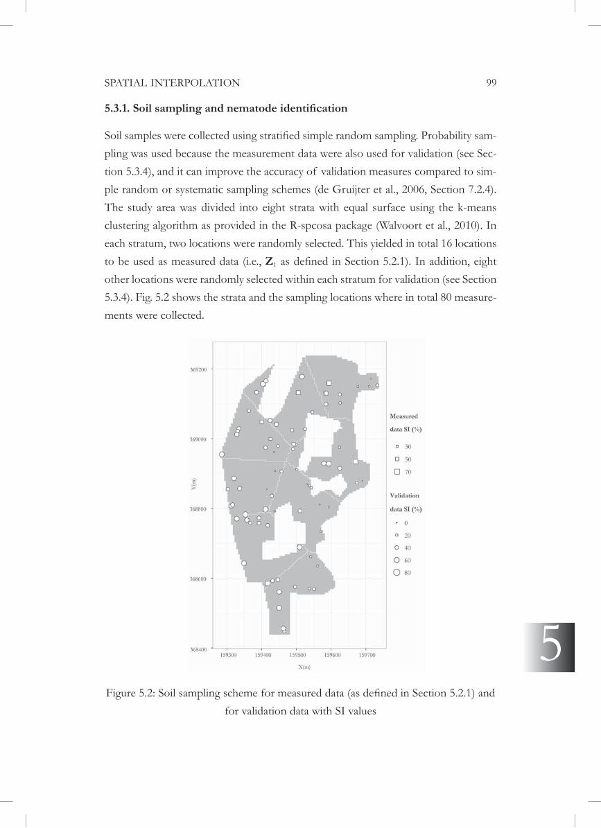
SPATIAL INTERPOLATION 99
5
-pling was used because the measurement data were also used for validation (see Sec-tion 5.3.4), and it can improve the accuracy of validation measures compared to sim-ple random or systematic sampling schemes (de Gruijter et al., 2006, Section 7.2.4).
clustering algorithm as provided in the R-spcosa package (Walvoort et al., 2010). In each stratum, two locations were randomly selected. This yielded in total 16 locations to be used as measured data (i.e., Z1
other locations were randomly selected within each stratum for validation (see Section 5.3.4). Fig. 5.2 shows the strata and the sampling locations where in total 80 measure-ments were collected.
for validation data with SI values
100 CHAPTER 5
5
Soil samples were collected on March 20th, 2013 at 0-20 cm depth using a 4 cm diameter soil corer. The nematodes in each of the 80 soil samples were extracted us-ing an Oostenbrink elutriator (Oostenbrink, 1960), within three weeks after sampling.
5.3.2. Sampling scheme for expert elicitation
For expert elicitation, we added 34 locations to the available 16 locations where meas-urements were taken to make in total 50 locations. The 34 additional locations were uniformly spread over the study area as well as at short distances to better infer short distance variation in all directions (we assumed isotropic variation because there is no reason for anisotropic variation of the regression residual). For this purpose, we
possible 19 sampling locations, conditional to the available 16 measurement locations. The remaining 15 locations were added at short distances (about 15 meters) from
measured data and 50 expert data) is accepted as an appropriate sample size for var-iogram inference using REML (Kerry and Oliver, 2007). Fig. 5.3 shows all locations for expert elicitation within the study area.
5.3.3. Expert elicitation procedure
A web-based tool11 was built to facilitate the expert elicitation procedure. Fig. 5.4 shows the main page of the web-based tool. We recruited one expert who is a soil ecologist with hands-on experience in nematode biomonitoring, including data in-terpretation. The expert has never visited the study area and received an allowance for the job. The expert was given access to the web-based tool where information about the study area, the sampling scheme, soil conditions of the study area (maps and tables, see Appendix 5.A, with soil properties: moisture content, organic matter content, pH-water, clay content, total concentrations of cadmium and zinc, elevation, and distance to river), and explanation of the probability expert elicitation procedure was given.
11http://variogram.isric.org/

SPATIAL INTERPOLATION 101
5
Figure 5.3: Sampling scheme for expert elicitation of nematode community indices: 1. Locations with measured and expert data (16 locations), 2. Locations with only
expert data (34 locations)
indicator values (O’Hagan, 1998; Bedford and Walls, 2010). The expert was asked to work on the exercise during one working day including getting familiar with the tool, the soil conditions in the study area, the statistical background on estimating the val-
st, 2013.
In Section 5.4, we report and analyse only the results of SI from the elicitation exercise because the EI did not show spatial correlation from the direct measure-ments. The soil properties that have a high correlation with SI from the direct meas-
the spatial trend of SI was modelled as a linear function of these three covariates:

102 CHAPTER 5
5
pH-water ƒ1 , soil moisture ƒ2 and organic matter content ƒ3 . The exhaustive maps of the three covariates over the study area (Fig. 5.5) to be used for regression were interpolated by ordinary kriging on nodes of a 5m-grid map covering the study area from 100 soil samples that were collected and analysed in 2008.
Figure 5.4: Main page of web-based tool for expert elicitation of nematode struc-
ture and enrichment indices
5.3.4. Accuracy assessment
-
deviation ( -
al., 2006, Section 7.2.4).

Figu
re 5
.5: E
xhau
stiv
e m
aps o
f SI
cov
ariat
es: p
H-w
ater
(lef
t), so
il m
oist
ure
(mid
dle)
and
org
anic
mat
ter c
onte
nt (r
ight
)
SPATIAL INTERPOLATION 10

104 CHAPTER 5
5
two measures:64
164 RCK
1RCK v
i=
s and64 2
164
1
ˆRCK RCK v v
i=
RMSE Z s Z s , where sv, v = 1, …, 64
are the validation locations. For the purpose of comparison, we also did regres-
sion kriging (RK) using only the measured data with the same three covariates (Sec--
RCK and RMSERK were also
RMSE RMSERCK RCK(RK) (RK). var± ( )1 998 -dent distribution with 63 degrees of freedom.
5.4. Results and Discussion
5.4.1. Expert data of SI
Fig. 5.6 shows the mean and standard deviation of SI that were calculated from the -
locations were given to help the expert distinguish the spatial differences, particularly between nearby locations, but this demanded the expert the ability to link and weigh all information in the judgements. The number of locations for which the expert gave
-ing the exercise. These two factors can also contribute to high uncertainty in expert
-
Fig. 5.6 (left) shows that nearby locations tend to have similar mean values of SI. The magnitude of the spatial autocorrelation is presented in Section 5.4.2. The mean values of the SI also show a slight trend with higher values in the west and lower values in the east. There is a slightly positive linear correlation (Pearson correlation

SPATIAL INTERPOLATION 105
5
SI. This means that the expert is more uncertain at locations where the expert thought that SI is large. At co-located locations, the mean values of the expert data are on
Z2 in
data at co-located locations is 0.11 (p-value = 0.347). This indicates a positive linear relationship between the measured data and the expected values of the expert data, but the correlation is not strong.
Figure 5.6: Nematode structure index estimated from expert judgements: mean value (left) and standard deviation (right)
The weak relationship between the mean values of SI from expert data and the measured data at co-located locations and high variation in SI values of expert data
values as Z2 and the standard deviation as is legitimate but apparently has conse-
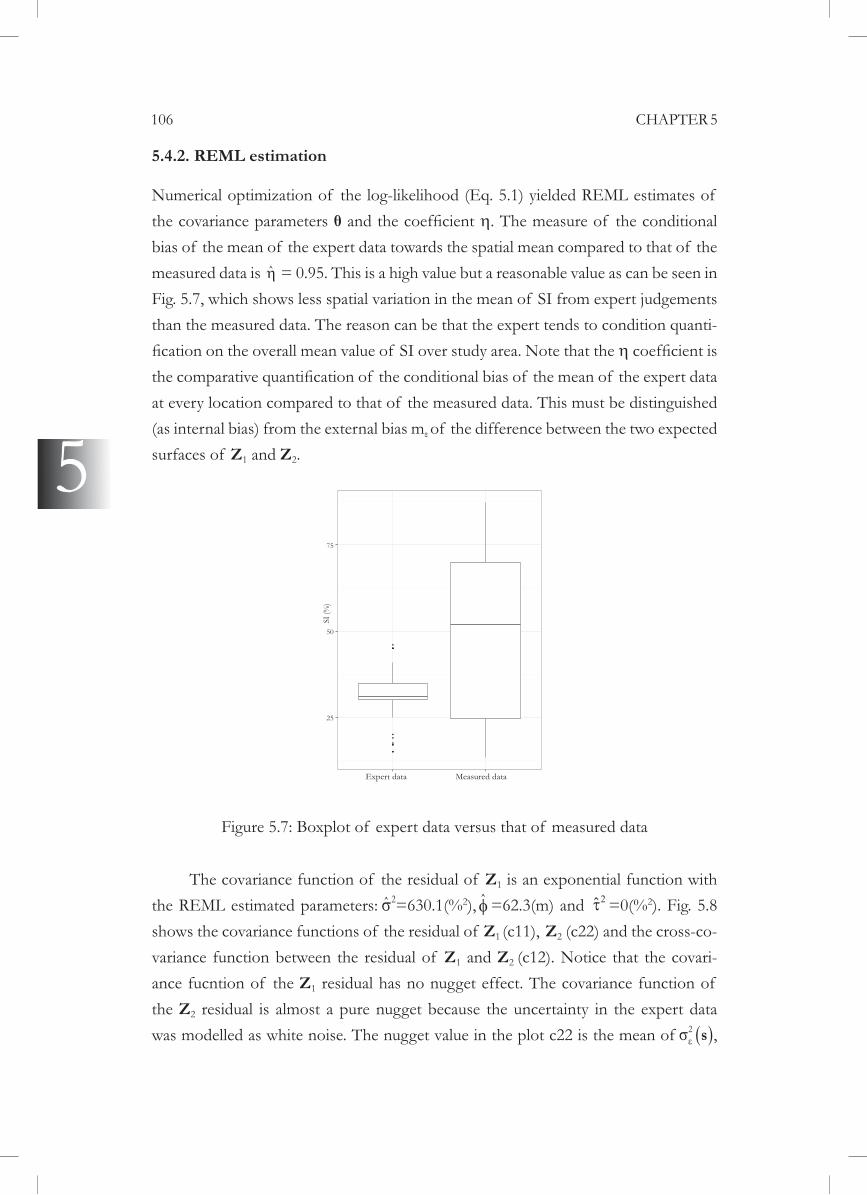
106 CHAPTER 5
5
5.4.2. REML estimation
the covariance parameters . The measure of the conditional bias of the mean of the expert data towards the spatial mean compared to that of the measured data is ˆ = 0.95. This is a high value but a reasonable value as can be seen in Fig. 5.7, which shows less spatial variation in the mean of SI from expert judgements
-
at every location compared to that of the measured data. This must be distinguished (as internal bias) from the external bias m of the difference between the two expected surfaces of Z1 and Z2.
Figure 5.7: Boxplot of expert data versus that of measured data
The covariance function of the residual of Z1 is an exponential function with the REML estimated parameters: 2ˆ 2), ˆ =62.3(m) and 2ˆ 2). Fig. 5.8 shows the covariance functions of the residual of Z1 (c11), Z2 (c22) and the cross-co-variance function between the residual of Z1 and Z2 (c12). Notice that the covari-ance fucntion of the Z1 residual has no nugget effect. The covariance function of the Z2 residual is almost a pure nugget because the uncertainty in the expert data was modelled as white noise. The nugget value in the plot c22 is the mean of 2 s ,

SPATIAL INTERPOLATION 107
5
Z1 is 1 10 11 12 13ˆ ˆ ˆ ˆ ˆ389.1, 85.2, 1.9, 4.6 and that of Z2 is
2 20 21 22 23ˆ ˆ ˆ ˆ ˆ89.8, 11.6, 0.5, 3.75 . Hence, the systematic bias of the ex-pert data is 1 2 3m 299.3 73.6 1.4 0.85s s s sf f f .
Figure 5.8: REML estimated covariance functions (c11, c22) and cross-covariance function (c12)
Fig. 5.9 shows the trends of SI from the two models on an arbitrary transect through the study area from west to east. The values were sorted from smallest to largest according to the mean values of Z1. It clearly shows that the expert data are
of the expert data for the SI has been smoothed over the study area: the high mean
condition of the RCK predictor (Journel and Huijbregts, 1978, Section V.A.4; Chilès
prediction.
OOOOOOOOOOOOOOOOOOOOOOOOOOOOOOOOOOOOOOOOOOOOOOOOOOOOOOOOOOOOOOOOOOOOOOOOOOOOOOOOOOOOOOOOOOOOOOOOOOOOOOOOOOOOOOOOOOOOOOOOOOOOOOOOOOOOOOOOOOOOOOOOOOOOOOOOOOOOOOOOOOOOOOOOOOOOOOOOOOOOOOOOOOOOOOOOOOOOOOOOOOOOOOOOOOOOOOOOOOOOOOOOOOOOOOOOOOOOOOOOOOOOOOOOOOOOOOOOOOOOOOOOOOOOOOOOOOOOOOOOOOOOOOOOOOOOOOOOOOOO
OOOOOOOOOOOOOOOOOOOOOOOOOOOOOOOOOOOOOOOOOOOOOOOOOOOOOOOOOOOOOOOOOOOOOOOOOOOOOOOOOOOOOOOOOOOOOOOOOOOOOOOOOOOOOOOOOOOOOOOOOOOOOOOOOOOOOOOOOOOOOOOOOOOOOOOOOOOOOOOOOOOOOOOOOOOOOOOOOOOOOOOOOOOOOOOOOOOOOOOOOOOOOOOOOOOOOOOOOOOOOOOOOOOOOOOOOOOOOOOOOOOOOOOOOOOOOOOOOOOOOOOOOOOOOOOOOOOOOOOOOOOOOOOOOOOOOOOOOOOO
OOOOOOOOOOOOOOOOOOOOOOOOOOOOOOOOOOOOOOOOOOOOOOOOOOOOOOOOOOOOOOOOOOOOOOOOOOOOOOOOOOOOOOOOOOOOOOOOOOOOOOOOOOOOOOOOOOOOOOOOOOOOOOOOOOOOOOOOOOOOOOOOOOOOOOOOOOOOOOOOOOOOOOOOOOOOOOOOOOOOOOOOOOOOOOOOOOOOOOOOOOOOOOOOOOOOOOOOOOOOOOOOOOOOOOOOOOOOOOOOOOOOOOOOOOOOOOOOOOOOOOOOOOOOOOOOOOOOOOOOOOOOOOOOOOOOOOOOOOOO

108 CHAPTER 5
5Figure 5.9: Difference in mean value (spatial trend) of SI from expert data versus
measured data over an arbitrary transect from east to west in the study area
5.4.3. RCK prediction and accuracy
Recall that the data used for RCK included 16 error-free measurements and 50 soft data. Fig. 5.10 shows the RCK prediction and standard deviation maps. The RCK pre-
the expert data were not reproduced exactly because these had error.
For the case of using only the measured data, RK predictions over the study area have a wider range of value of the standard deviation than that of RCK (i.e.
a large amount of the kriging variance at locations farther away from exact meas-urements. At the 64 validation locations, RCK RCK
while for the case of using only measured data, RK RK = 24.3 2
RCK

SPATIAL INTERPOLATION 109
5
RMSERK -ence in the performance of RCK compared to that of RK. Fig. 5.11 shows a scatter plot of the prediction error of RCK versus that of RK at the validation locations.
Figure 5.10: Regression cokriging of SI using expert data and measured data: kriging prediction (left) and kriging standard deviation (right)
The validation results showed no improvement in the prediction accuracy when -
relation between expert and measured data and the contrast in the nugget effect be-tween the residual covariance functions of the two datasets. As a result, the RCK weights of the expert data were very small compared to that of the measured data (Asli and Marcotte, 1995; Goovaerts, 1997, Section 6.2). The RCK system assigned
-iance of the estimated trend at locations without direct measurements is the main reason that caused a large reduction of the RCK standard deviation. Similar results have been observed in the study of Stein and Corsten (1991).

110 CHAPTER 5
5Figure 5.11: Regression cokriging prediction error versus regression kriging predic-
tion error at validation locations
5.5. Conclusions
In this study, expert judgements based on expert knowledge about the values of a
measurements in geostatistical prediction. This has not been the only work that at-tempted to make use of information from experts for geostatistical prediction (other examples are Omre (1987), Okx et al.(1991), Stein (1994), Chapters 2 - 3), but this is
knowledge was extracted by a formal statistical expert elicitation procedure. By using
experts in a probabilistic form.
The geostatistical models were built not only for incorporating expert knowl-
provided the tool to validate expert judgements by measures of the systematic bias,

SPATIAL INTERPOLATION 111
5
the conditional bias and random error. The case study indicated that when expert data are treated as soft data that have large random errors, inclusion of expert data has no
cannot improve the prediction accuracy. However, this conclusion must be adhered
in this study. Future research may investigate different ways of specifying the model
increasing the number of experts sharing knowledge) on the prediction accuracy. One
Appendix 5.A. Soil condition and expert judgements at 50 locations
Loc pH Clay OC Moist Disri Elev Cdtot Zntot LQ UQ1 4.09 0.56 2.30 18.45 136 27.29 0.26 8 20 402 4.10 0.64 3.54 17.22 289 27.43 0.34 12 30 503 4.42 1.39 6.66 39.39 143 26.50 2.10 81 20 404 4.75 11.15 14.11 72.78 13 26.38 73.64 1,326 15 255 4.79 0.88 4.98 36.24 63 27.00 2.83 116 25 406 4.78 1.69 7.15 44.84 18 26.84 8.08 214 20 407 4.72 1.74 5.38 37.19 73 27.16 5.17 140 25 408 4.18 0.56 2.65 14.95 167 27.54 0.41 15 40 509 4.72 4.80 10.85 65.54 21 26.64 55.44 753 23 30
10 4.08 1.10 2.71 17.57 197 27.33 0.15 10 30 5011 4.34 1.07 4.00 27.38 178 26.88 0.55 31 20 4012 4.46 0.92 6.12 31.50 154 27.15 2.78 81 25 4513 4.49 3.49 12.60 72.45 69 26.69 13.11 313 25 3514 4.75 8.82 15.55 80.74 33 26.57 30.27 561 20 3015 4.46 1.62 7.87 45.41 105 26.63 4.15 81 25 3516 4.48 0.57 5.69 32.29 161 26.63 1.66 51 25 3517 4.48 1.37 6.60 44.39 100 26.56 6.46 105 23 4418 4.55 0.60 5.74 30.22 204 26.88 1.55 75 25 4519 4.55 8.63 16.76 87.67 24 26.46 29.27 509 20 3020 4.61 10.09 14.55 79.62 20 26.48 30.28 661 20 3021 4.17 1.63 2.38 16.60 231 26.90 0.05 6 20 4022 4.30 1.04 2.96 13.64 310 27.20 0.42 29 30 5023 4.28 0.68 5.48 30.42 268 27.05 0.77 30 25 4024 4.58 0.85 3.56 24.58 276 26.39 0.53 31 30 50

112 CHAPTER 5
5
Loc pH Clay OC Moist Disri Elev Cdtot Zntot LQ UQ25 4.63 1.14 10.65 55.22 180 26.49 4.11 185 25 4026 3.60 1.88 3.92 15.62 271 27.95 0.31 13 20 4527 4.09 0.57 4.11 17.30 331 27.25 0.56 22 30 5028 4.57 2.54 8.58 57.66 111 26.43 11.74 190 20 4129 4.72 11.15 14.95 76.45 35 26.35 66.18 1,023 10 2530 4.45 1.47 6.85 44.21 164 26.45 1.99 68 25 4031 4.82 8.68 13.56 68.20 71 26.31 98.35 1,743 10 2032 4.61 3.34 11.20 60.20 87 26.30 23.05 476 15 2333 4.46 0.57 7.13 43.57 243 26.62 0.84 56 25 4034 4.47 2.14 7.24 44.01 49 26.49 7.39 126 23 4435 4.35 0.66 2.81 20.14 136 27.45 0.63 24 32 5036 4.26 0.59 2.70 17.20 152 27.45 0.50 19 40 5037 4.22 0.57 2.67 15.95 159 27.47 0.45 17 40 5038 4.30 0.62 2.74 18.62 144 27.46 0.56 21 42 5039 4.70 5.15 11.98 61.64 81 26.35 49.75 877 13 2140 4.78 6.54 12.63 64.35 82 26.33 70.66 1,259 10 2041 4.64 4.14 11.54 60.10 83 26.33 35.13 639 13 2142 4.40 0.65 6.25 37.61 255 26.69 0.78 49 23 3943 4.37 0.70 5.93 33.97 261 26.74 0.84 44 23 3944 4.39 0.58 6.52 41.26 249 26.67 0.65 47 23 3945 3.87 1.48 3.02 13.73 249 27.19 0.22 13 20 4046 3.72 1.69 3.52 14.60 260 27.80 0.30 14 20 4047 4.01 1.42 2.61 14.08 240 27.04 0.11 10 20 4048 4.49 1.49 7.08 45.39 72 26.50 5.11 96 25 4549 4.48 1.52 7.01 43.95 59 26.53 5.03 94 24 4550 4.49 1.49 6.96 45.64 87 26.56 5.71 102 24 45
Loc = locations, pH = pH-waterDisri = Distance to river (meter), Elev = Elevation asl (meter), Cdtot
= Cd total concentration (mg/kg), Zntot = Zn total concentration (mg/kg), LQ =
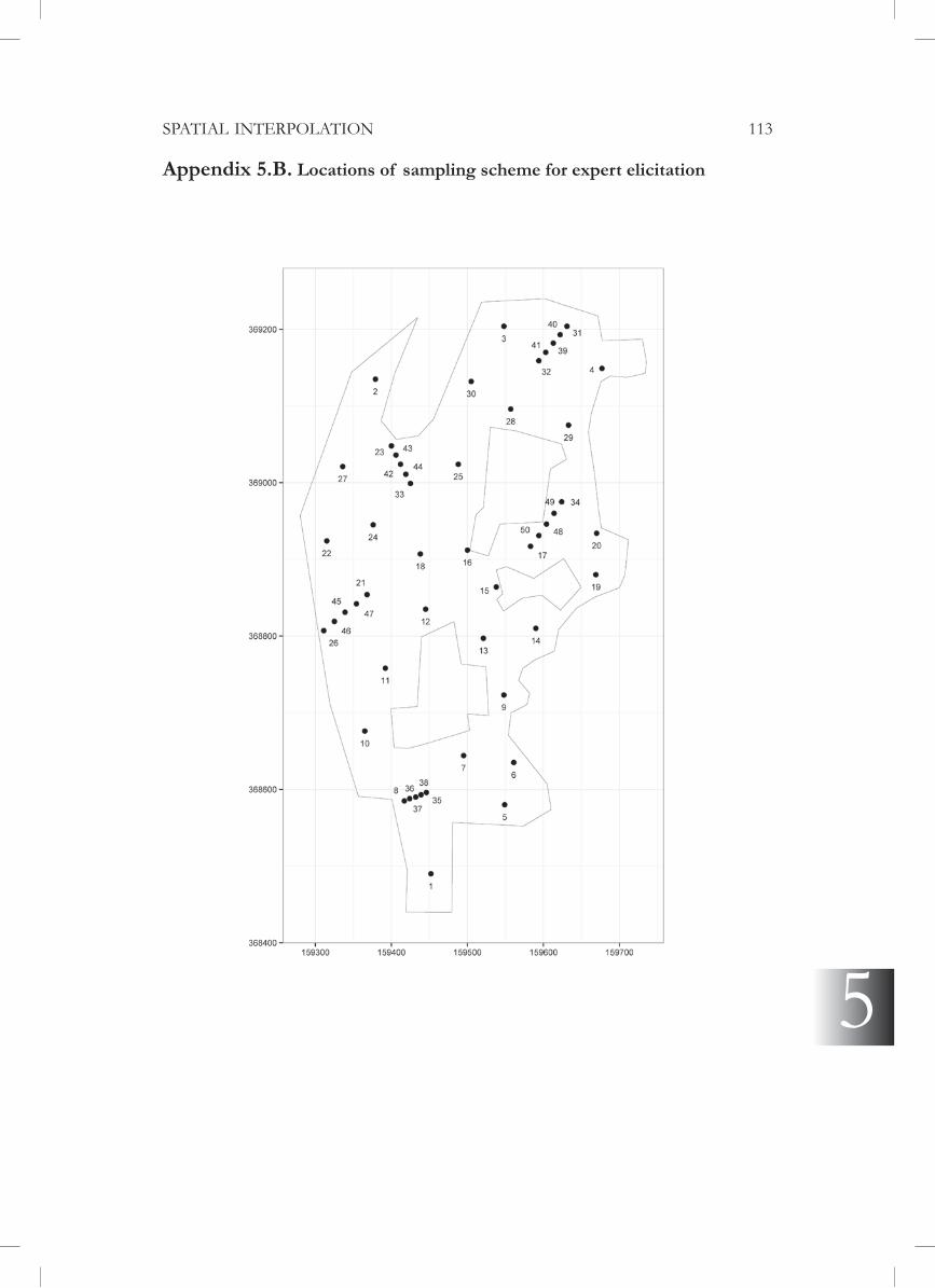
SPATIAL INTERPOLATION 113
5
Appendix 5.B. Locations of sampling scheme for expert elicitation


General discussion
Chapter 6

116 CHAPTER 6
6
6.1. Introduction
Geostatistics is increasingly used in numerous disciplines of the Earth and environ-mental sciences and in practical problem-solving, along with the increased urge to advance our understanding of the Earth surface and subsurface spatial phenomena.
or collect more (direct and ancillary) data and information. In this dissertation, I have gone for the second approach that seeks for more data and information. In my case, the source of more data and information is expert knowledge. Due to this, I also had to modify the geostatistical models that incorporate expert knowledge because using
-
-cal research for data and information that cannot be sensibly obtained using physical measurement systems, the rapid developments in expert elicitation research and the availability of increasingly knowledgeable experts working in geostatistical research and other disciplines within the Earth and environmental sciences. These factors not
This chapter synthesises the main accomplishments of the work that I have done and that were presented in the previous chapters: to identify the role of ex-pert knowledge in geostatistical research and to offer methods to elicit and incorpo-rate expert knowledge in geostatistical inference and prediction. While the foregoing
is the role of expert knowledge in geostatistical inference and prediction?, 2. How to elicit and incorporate expert knowledge in geostatistical inference and prediction?
-ence and prediction. Section 6.3 provides the answer to the second main research
expert knowledge in geostatistical models. Section 6.4 provides my personal view and discussion about how to advance this research topic. Finally, concluding remarks are given in Section 6.5.

GENERAL DISCUSSION 117
6.2. What is the role of expert knowledge in geostatistical inference
and prediction?
6.2.1. The role of expert knowledge in geostatistical inference and prediction
The geostatistical literature shows that expert knowledge has been marginally and informally used so far for geostatistical inference and prediction. When geostatistical data and information are unattainable (promptly and conveniently), the only remain-ing option is to ask for expert opinions. Several situations where expert knowledge
structure inference (i.e. variogram estimation described in Chapters 2, 3, 4 and 5, and spatial trend estimation addressed in Chapter 5), spatial interpolation (Chapters 4
(Chapter 4). These situations can be categorised into cases of: 1. inaccessible or unat-
The data and information gaps recognised in this research are: information about the spatial structure to use as prior information or forecast (Chapter 2), data for spatial
-mation about the spatial structure at a different spatial support (Chapter 4) and spatial gaps in the measurements for the variogram and spatial trend inference and kriging (Chapter 5).
Throughout this research, expert knowledge has been used not only as prior information but also as (soft) data. The formal roles of expert knowledge in geosta-
Drescher et al. (2013): as surrogate for absent geostatistical data to infer the variogram
poorly captured by conventional mapping methods (Chapter 3), as complementary data
(Chapter 4), and as supplement to measured data to enhance inference and prediction (Chapter 5).
judgement. This is the type of data and information that geostatisticians need for

118 CHAPTER 6
6
of geostatistical data, and this analysis is subject to uncertainty. The role of expert
in other research disciplines such as geology (Wood and Curtis, 2004; Curtis, 2012), landscape ecology (Perera et al., 2012b; Drescher et al., 2013), environmental health impact assessment (Knol et al., 2010), and environmental modelling and management (Krueger et al., 2012). The marginal and informal use of expert knowledge in geosta-tistics has been replaced in this research by a formal and systematic use. This formal use enhances the added value of expert knowledge because the expert elicitation pro-cedure is formalised and explicitly reported. Hence, the validity of expert judgement can be monitored and assessed.
dependence on location or area, i.e. the knowledge used is about the spatial variability
to have knowledge that can be used to infer the spatial correlation structure of a
in using expert knowledge in geostatistical inference and prediction, besides other -
ley, 1975; Meyer and Booker, 2001). As mentioned in Chapter 2, there are limited
the second-order moment (i.e. the variance) (Cressie, 1991, Section 2.3.1; Oliver et al., 2010a). Expert elicitation literature indicates that experts are subject to cognitive
-mation in two dimensions: spatial space and attribute space. As a result, it is more dif-
-ences reported in Chapter 3 where experts were asked to judge the spatial structure of
-dane and Wolfson, 1998). Another aspect is that local expert knowledge might out-

GENERAL DISCUSSION 119
weigh general expert knowledge in a geostatistical context because local and detailed
the data used in geostatistics. Besides the case shown in Chapter 4, another clear ex-
locations within a given area. The high uncertainty in the expert judgements is good
My research also showed that expert knowledge cannot be helpful in all cases, as also stated in Kuhnert et al. (2010) and Kuhnert (2011). Its usefulness is determined
knowledge. The former is determined by all factors that build the elicitation proce-dure (e.g. see Knol et al., 2010), while the latter might be dependent on the domain expert (not the elicitation expert). Chapter 5 gives an example of the unsuccessful use of expert knowledge to improve spatial inference and prediction. The reasons for
knowledge from the expert. Natural scientists might encounter this obstacle when they work with experts because they may lack social and psychological skills. This important point will be further discussed in Section 6.3. It is also suggested to use a better approach than directly eliciting the values of the variable at multiple locations, because this long and intensive knowledge extraction procedure can be tiring (Miller, 1956). Another reason for the disappointing results in Chapter 5 might be that single expert knowledge is not satisfactory in all cases.
Indeed, using knowledge from a single expert can be risky and is only recom-mended in the case of testing new elicitation methods. However, in practice, there might not be many experts, particularly in geostatistics where the experts are ex-
-cept for one of the co-authors. As emphasised in the expert elicitation literature (e.g. O’Hagan, 2012; Drescher et al., 2013), this research corroborates that uncertainty in expert knowledge and judgement must be taken into account. Otherwise, the use of
in each expert judgement, which was done in Chapter 5. Another way is to consult
120 CHAPTER 6
6
multiple experts where all of the differences in expert knowledge are taken into ac-count (Chapters 2, 3 and 4). When expert data are integrated with measured data at the same spatial support (i.e. the expert knowledge plays a supplement role), there can be a (complete) overlap between measured data and expert knowledge if the knowl-edge has been accumulated based on available measured data published elsewhere.
due to its geographical dependence, the two dimensional information processing -
tiple experts and uncertain expert knowledge. Note that the discussion in this section
using expert knowledge to identify relevant models, data sources, types of knowledge, etc. (Booker et al., 2001)) has not been investigated in this research. In spite of the
that expert knowledge can be very meaningful. Having recognised this, the challenges
discusses some mechanisms to tackle these challenges.
6.3. How to elicit and incorporate expert knowledge in geostatisti-
cal inference and prediction?
In this research, I have been working on geostatistical analysis of only spatial datasets of natural phenomena, and they are collected from measurements and expert knowl-edge. The aims of using geostatistical analyses are to statistically analyse the spatial
6.3.1. Statistical expert elicitation in a geostatistical context
-tributions were used to extract expert knowledge, but expert judgements were used
-tion of random variables indexed by spatial coordinates (Schabenberger and Gotway,
-

GENERAL DISCUSSION 121
tistical settings. The model-based geostatistical approach (Diggle and Ribeiro, 2007) was applied throughout this research by explicitly assuming the underlying process of the spatial phenomena as normal or log-normal multivariate distributions. Hence, the
distribution. Although there are elicitation methods for the multivariate probability distribution, these are far too complicated and inappropriate to be applicable to the geostatistical setting. Nevertheless, the elicitation method in this research was devel-oped based on the same principle that is used in the expert elicitation literature for multivariate distributions (e.g. Al-Awadhi and Garthwaite, 1998; O’Hagan et al., 2006, Section 5.3). The method includes two components (Chapters 2 and 3): the elicitation
-alent to the elicitation of the association in the expert elicitation literature).
A systematic and formal procedure was used to develop the expert elicitation tasks in each of the four case studies (Section 1.5.1) of which the core component of the elicitation facilitator is a web-based tool. This formal procedure (e.g. as used in Chapter 3) completely followed recommended procedures recently published in the expert elicitation literature (e.g. Choy et al., 2009; Knol et al., 2010; Kuhnert et al., 2010), although the web-based tools were newly built in Chapters 2, 3 and 5. One
expertise of the facilitator but also social skills (interpersonal skills) that can be a main obstacle for a natural scientist. Some previous investigations on this task also share the same experience, e.g. as reported in Drescher et al. (2013). The most laborious task is designing the elicitation tool, and this task is distinct among different research disciplines. The other tasks more or less stay unchanged as in the recommended pro-cedure when applied in geostatistical setting.
-
-
parameters (i.e. the parameters of the Matérn variogram model in Chapter 4) and

122 CHAPTER 6
6
being elicited: the indirect method was used in Chapters 2 and 3 and the direct meth-od in Chapters 4 and 5. As recommended in the expert elicitation literature (e.g. Choy
-pert. The domain experts in this case are demanded to use their expertise to identify
The web-based elicitation tools were developed for both one and multiple ex-perts’ elicitation. In case of multiple expert elicitation, the Delphi method was used where the experts were anonymous to each other, and only the combined expert judgement was revealed to all experts (Cooke, 1991, Section 3.3.1; Kuhnert et al., 2010). The purpose was to seek for a consensus among multiple experts, except in
-ly weighs the knowledge of the experts was used to combine multiple experts’ judge-
pragmatic reason (i.e. simple use and debate, taking into account all expert opinions
opinion. One of the main reasons is that I am not convinced by other more com-plicated approaches (i.e. the Bayesian method, weighted pooling, etc.) in terms of reaching a better representation of expert consensus. This sceptical point of view also appears in other studies (e.g. Clemen and Winkler, 1999; Clemen, 2008; Kuhnert et al., 2010). The technical solution for implementation of a web-based tool is limit-
Cooke’s classical methods (Cooke, 1991) were used. Another reason for mathematical
experts (Chapters 2 and 3) and to use the maximum diversity of the expert opinions to consider all experts’ uncertainty (Chapter 4).
When developing the elicitation tools, I paid much attention to controlling the (cognitive) biases in expert judgements because it is a severe problem in using expert knowledge. My work was aimed at not only raising awareness of the experts them-
minimising the biases at some stages of the elicitation procedure. For example, the

GENERAL DISCUSSION 123
method with anonymous experts was used to prevent motivational biases. This is also
knowledge from psychology and decision theory. Regardless of all the effort, the self-de-biased capability of experts might play a decisive role, particularly in the context of individual self-elicitation using web-based tools.
The role of the facilitator is always important (e.g. as proven Section 3.4), re-gardless which elicitation approach used (i.e. interview, workshop, web-based, etc.).
-pert and the elicitation facilitator or elicitator. The responsibility of the domain expert is on the domain knowledge (i.e. geostatistical knowledge in this research), and that of
of both the domain expert and the elicitator (as done in my case) demands a double effort; and hence, drawbacks are inevitable (e.g. the revision of expert judgement in Chapter 3, a large uncertainty in the elicitation outcome of one expert in Chapter 5). To apply expert elicitation theory in a geostatistical context, geostatistical background is a ‘must’ condition, while expert elicitation knowledge is an ‘enough’ condition to obtain a successful task; and again all frustrations that may turn up are due to the fact that working with human knowledge is a more complex and totally different situation
-cians and the elicitation experts is recommended.
In this research, I have developed practically rigorous expert elicitation ap-proaches that satisfy two criteria: incorporating a measure of uncertainty for the elic-ited expert knowledge and including an assessment of internal or external validity of
other chapters, where expert uncertainty was taken into account, and the internal and external biases of expert judgements were measured; hence, validity of the kriging map was assessed. This is an effort that should be stimulated, even though the results of this chapter are provisionally frustrating.
6.3.2. Methods of expert knowledge incorporation in geostatistics
To incorporate expert knowledge in geostatistical inference and prediction, two par-adigms were leading this research: expert knowledge as prior information under a Bayesian perspective (i.e. Bayesian area-to-point kriging in Chapter 4) and as (soft)

124 CHAPTER 6
6
-ter 5). The important consideration for incorporating expert knowledge in geosta-tistical models is about the inexact or uncertain nature of judgements. The Bayesian
to include uncertainty about the model parameters in kriging (Pilz and Spock, 2008) and combine data from different spatial supports (Gotway and Young, 2002). When expert data are integrated with measured data (either at the same or a different spatial support), properly weighing the contribution of expert knowledge in inference and prediction compared to that of the measured data may be of most concern. This weighing system should be controlled by the size of the dataset, the overlap between
-tances. In this regard, both paradigms can be satisfactory.
Geostatistical models are usually well-prepared to integrate incompatible data-sets (see e.g. Goovaerts, 1997, Chapter 6; Gotway and Young, 2002 for an overview). This statement is made based on the fact that all geostatistical models that were used to incorporate expert knowledge in this research are available in the literature. The
that are integrated (e.g. Chapter 5). However, this can be a biased statement because
experts, less work is demanded on ‘reinventing’ geostatistical models. A better com-prehensive approach can be to ask the expert what knowledge they can best provide and then modify the geostatistical models to best use these knowledge. The evolu-tion of a hierarchical perspective in spatial-temporal geostatistics (Cressie and Wikle,
In summary, while elicitation of expert knowledge in geostatistics may be ac-complished by following an existing formal elicitation procedure with a new elicita-
in geostatistical inference and prediction may make use of the Bayesian and the ge-ostatistical approaches. Note that all the comparisons made so far are based on the

GENERAL DISCUSSION 125
literature from other research disciplines because no previous research on expert elic-itation in geostatistics has been published.
6.4. Insight and Implications
6.4.1. Expert knowledge through the eye of geostatisticians
Geostatisticians might look at expert knowledge of a spatial variable as a (linear) regression prediction (with error) because they might expect that experts can relate their judgements to the factors in the environment that affect the distribution of the spatial variable. They might even think that experts make a simple extrapolation in their judgements when they judge the value at unobserved locations. When knowl-
extract these only from the geostatistical specialists. These preliminary views are my personal, and the geostatisticians that I have in mind are geostatistical practitioners. This view may help experts understand the expectation when they are involved in a geostatistical elicitation task.
6.4.2. The interaction between geostatistical models and expert knowledge
geostatistics and the geostatistical models that can incorporate expert knowledge. On
from experts was shaped in one way or another by geostatistical assumptions. For ex-ample, the marginal distribution of a random spatial variable was limited to be either normal or log-normal (Chapters 2 and 3), and the intrinsic and isotropic variogram model was elicited (Chapter 4). All of the basic assumptions of geostatistical mod-els (i.e. (log-) normal probability distributions, (second-order or intrinsic) stationary, isotropy) were either explicitly or implicitly imposed on the expert judgements. To a certain extent, these imposed assumptions on the experts and their judgements are
to say that geostatisticians have formed their knowledge about spatial phenomena in this way, and hence, the same expectation holds for the knowledge of other experts of applied geostatistics.
-ostatistical models was not considerable in this research. Some limitations that were
126 CHAPTER 6
6
appropriate any more (Chapter 2), and that kriging should consider the error in the data (Chapter 5). I argue that the better expert knowledge is the one that is not limited by geostatistical assumptions; otherwise, besides the possible (motivational) bias, the overlap between expert knowledge and published data and information can be large, which lessens the added value of expert knowledge. It is interesting but not trivial to investigate what knowledge humans actually hold about a spatial phenomenon. Hu-man knowledge is much more than a geostatistical sample. A different geostatistical model is thus need to sensibly make better use of the data and information given by the expert judgements.
6.4.3. The possibility of expert judgement calibration and validation by geo-
statistical models
-
Chapter 8). They are not necessarily related. The former has been discussed in the previous four chapters, in the implementation of the elicitation procedures. In this section, only the calibration and validation of expert judgements are of concern. This is the assessment of an agreement between expert judgments and reality in a geosta-tistical context (O’Hagan et al., 2006).
I argue that expert judgments of a spatial variable should be better calibrated
6.3, while the experts judge the univariate probability distributions, their probabilistic -
tion of the individual univariate probability distribution are inappropriate because the (auto) correlation of the judgements matters. In case the expert judgements are the model parameters directly, the outcomes of the geostatistical models should be used. The case studies presented in this research demonstrate the possibility of using geo-statistical models for expert judgement calibration and validation.
-
ena
In Chapters 2 and 3, I have argued for the necessary assistance of computer software in statistical expert elicitation. Henceforth, all elicitation tasks in this research were

GENERAL DISCUSSION 127
assisted by computer software, and they all are web-based tools. Numerical optimiza--
tation outcomes, for example is a favourite aid of computer software. The visual aids
in the form of a spatial map; and web-mapping technology is already that much ad-vanced that it can be greatly advantageous.
-sive due to allowance and relocating cost in case recruited experts are geographically scattered. As a result, it can be costly (or even impossible) to gather multiple (busy)
can be web-based operationalised (e.g. Morris et al., 2014). The remote elicitation ex-
when it is established, it provides a long term use.
6.4.5. Future research challenge
The important challenge for future researchers on this topic lies in how to maximise -
with interdisciplinary knowledge and skills. The challenge is worth the effort because
their knowledge about them is often of high value.
6.5. Conclusions
1. The added value of expert knowledge in geostatistical inference and prediction is real.
2. The use of statistical expert elicitation to extract knowledge from experts is essential to enhance the use of expert knowledge in geostatistics.
3. Expert knowledge should ideally be elicited freely from geostatistical assump-tions, and the geostatistical model should be well-prepared for integrating elicited knowledge.


REFERENCES 129
References
Al-Awadhi, S.A., Garthwaite, P.H., 1998. An elicitation method for multivariate nor-mal distributions. Commun. Stat. Theory Methods 27, 1123 - 1142.
Albert, J., 2009. Bayesian computation with R. Springer, New York.
Armstrong, M., 1998. Basic linear geostatistics. Springer, Berlin.
Asli, M., Marcotte, D., 1995. Comparison of approaches to spatial estimation in a bivariate context. Math. Geol. 27, 641-658.
Atkinson, P.M., 2013. Downscaling in remote sensing. Int. J. Appl. Earth Obs. Geo-inf. 22, 106-114.
Ayyub, B.M., 2001. Elicitation of expert opinions for uncertainty and risk. CRC Press, Boca Raton, Florida.
Barnes, R., 1991. The variogram sill and the sample variance. Math. Geol. 23, 673-678.
linear models. Proc. Inst. Mech. Eng. O J. Risk Reliab. 224, 322-332.
Booker, J.M., Anderson, M.C., Meyer, M.A., 2001. The role of expert knowledge in -
standing?) Seventh army conference on applied statistics, 155-161.
Bowley, A.L., 1920. Elements of statistics. P.S. King & Son Limited, London.
Brus, D.J., Heuvelink, G.B.M., 2007. Optimization of sample patterns for universal kriging of environmental variables. Geoderma 138, 86-95.
Brus, D.J., Kempen, B., Heuvelink, G.B.M., 2011. Sampling for validation of digital

130 REFERENCES
soil maps. Eur. J. Soil. Sci. 62, 394-407.
Chesley, G.R., 1975. Elicitation of subjective probabilities: a review. Account. Rev. 50, 325-337.
Chib, S., Greenberg, E., 1995. Understanding the Metropolis-Hastings algorithm. Am. Stat. 49, 327-335.
series in probability and statistics. Wiley, New York.
Choy, S.L., O’Leary, R., Mengersen, K., 2009. Elicitation by design in ecology: using expert opinion to inform priors for Bayesian statistical models. Ecology 90, 265-277.
Clemen, R., Winkler, R., 1999. Combining probability distributions from experts in risk analysis. Risk Anal. 19, 187 - 203.
Clemen, R.T., 2008. Comment on Cooke’s classical method. Reliability Engineering & System Safety 93, 760-765.
Cooke, R.M., 1991. Experts in uncertainty: opinion and subjective probability in sci-ence. Environmental ethics and science policy series. Oxford University Press, New York.
Cooke, R.M., Goossens, L.H.J., 2000. Procedures guide for structured expert judge-
17, 563-586.
Cressie, N., 1990. The origins of kriging. Math. Geol. 22, 239-252.
Cressie, N., 1991. Statistics for spatial data. Wiley series in probability and mathe-matical statistics. Wiley, New York.
-ogr. Syst. 3, 159-180.
Cressie, N., Hawkins, D., 1980. Robust estimation of the variogram: I. Math. Geol.
REFERENCES 131
12, 115-125.
Cressie, N., Wikle, C.K., 2011. Statistics for spatio-temporal data. Wiley series in probability and statistics. Wiley, Oxford.
Cui, H., Stein, A., Myers, D. E., 1995. Extension of spatial information, Bayesian kriging and updating of prior variogram parameters. Environmetrics 6, 373-384.
Curtis, A., 2012. The science of subjectivity. Geology 40, 95-96.
De Goede, R.G.M., Bongers, T., Ettema, C.H., 1993. Graphical presentation and in-terpretation of nematode community structure: c-p triangles. Med. Fac. Land-bouww. Univ. Gent 58/2b: 743-750.
De Gruijter, J.J., Bierkens, M.F.P., Brus, D.J., Knotters, M., 2006. Sampling for natu-ral resource monitoring. Springer-Verlag Berlin Heidelberg: Berlin, Heidelberg.
Dowd, P.A. (Eds.), Geostatistical simulations: Proceedings of the Geostatisti-cal simulation workshop 7, Fontainebleau, pp. 131-145.
DeGroot, M.H., 1974. Reaching a consensus. J. Am. Stat. Assoc. 69, 118-121.
Denham, R., Mengersen, K., 2007. Geographically assisted elicitation of expert opinion for regression models. Bayesian Anal. 2, 99-136.
Dietrich, C.R., Newsam, G.N., 1993. A fast and exact method for multidimensional gaussian stochastic simulations. Water. Resour. Res. 29, 2861-2869.
Diggle, P.J., Ribeiro, Jr.P.J., 2002. Bayesian inference in Gaussian model-based geo-statistics. Geographical and Environmental Modelling 6, 129-146.
Diggle, P.J., Ribeiro, P.J., 2007. Model based geostatistics. Springer Series in Statistics, Springer, New York.
Dowd, P.A., 1984. The variogram and kriging: robust and resistant estimators, in: Verly, G., David, M., Journel, A.G. (Eds.), Geostatistics for natural resources characterisation (Part 1), pp. 91-106.

132 REFERENCES
Drescher, M., Perera, A.H., Johnson, C.J., Buse, L.J., Drew, C.A., Burgman, M.A., 2013. Toward rigorous use of expert knowledge in ecological research. Eco-sphere 4, art83.
Dungan J.L., 2006. Toward a comprehensive view of uncertainty in remote sensing analysis, in: Foody, G.M., Atkinson, P.M. (Eds), Uncertainty in remote sensing and GIS, John Wiley & Sons, Ltd, pp. 25-35.
Ettema, C.H., Wardle, D.A., 2002. Spatial soil ecology. Trends Ecol. Evol. 17, 177-183
Ferris, H., Bongers, T., de Goede, R.G.M., 2001. A framework for soil food web di-agnostics: extension of the nematode faunal analysis concept. Appl. Soil Ecol. 18, 13-29.
Fisher, R., O’Leary, R.A., Low-Choy, S., Mengersen, K., Caley, M. J., 2012. A soft-ware tool for elicitation of expert knowledge about species richness or similar counts. Environ. Model. Softw. 30, 1-14.
French, S., 2011. Aggregating expert judgement. Serie A. Matematicas 105, 181-206.
Frogbrook, Z. L., 1999. The effect of sampling intensity on the reliability of predic-tions and maps of soil properties. Precision agriculture ‘99, Part 1 and Part 2. 2nd European conference on Precision agriculture, Odense, Denmark, 11-15 July 1999.
Garthwaite, P.H., Dickey, J.M., 1985. Double- and single-bisection methods for sub-jective probability assessment in a location-scale family. J. Econom. 29, 149-163.
Garthwaite, P.H., Kadane, J.B., O’Hagan, A., 2005. Statistical methods for eliciting probability distributions. J. Am. Stat. Assoc. 100, 680-700.
Gelfand, A.E., Zhu, L., Carlin, B.P., 2001. On the change of support problem for spatio-temporal data. Biostatistics 2, 31-45.
Genest, C., Mcconway, K.J., 1990. Allocating the weights in the linear opinion pool. J. Forecast. 9, 53-73.

REFERENCES 133
Geweke, J., 1992. Evaluating the accuracy of sampling-based approaches to calcu-lating posterior moments, in: Bernardo, J.M., Berger, J.O., Dawid, A.P., Smith, A.F.M. (Eds), Bayesian statistics 4. Oxford University Press, pp. 169-193.
Goovaerts, P., 1997. Geostatistics for natural resources evaluation. Oxford Universi-ty Press, New York.
Goovaerts, P., 1999. Geostatistics in soil science: state-of-the-art and perspectives. Geoderma 89, 1-45.
Goovaerts, P., 2001. Geostatistical modelling of uncertainty in soil science. Geoder-ma 103, 3-26.
Goovaerts, P., 2008. Kriging and semivariogram deconvolution in the presence of irregular geographical units. Math. Geosci. 40, 101-128.
Goovaerts, P., Kerry, R., 2010. Using ancillary data to improve prediction of soil and crop attributes in precision agriculture, in: Oliver, M.A. (Ed), Geostatistical applications for precision agriculture. Springer Netherlands, Dordrecht, pp. 167-194.
Gotway, C.A., Young, L.J., 2002. Combining incompatible spatial data. J. Am. Stat. Assoc. 97, 632-648.
Gotway, C.A., Young, L.J., 2007. A geostatistical approach to linking geographically aggregated data from different sources. J. Comput. Graph. Stat. 16, 115-135.
Ha, W., Gowda, P., Howell, T., 2013. A review of downscaling methods for remote sensing-based irrigation management: part I. Irrigation. Sci. 31, 831-850.
Hahn, E.D., 2006. Re-examining informative prior elicitation through the lens of Markov chain Monte Carlo methods. J. R. Stat. Soc. Ser. A Stat. Soc. 169, 37-48.
Hall, D.G.M., Reeve, M.J., Thomasson, A.J., 1977. Water retention, porosity and den--
mental Station, Harpenden.

134 REFERENCES
Hamzehpour, N., Eghbal, M.K., Bogaert, P., Toomanian, N., Sokouti, R.S., 2013. Spatial prediction of soil salinity using kriging with measurement errors and probabilistic soft data. Arid Land Research and Management 27, 128-139.
Hengl, T., Heuvelink, G.B.M., Rossiter, D.G., 2007. About regression-kriging: From
Heuvelink, G.B.M., 2006. Analysing uncertainty propagation in GIS: Why is it not that simple?, in: Foody, G.M., Atkinson, P.M. (Eds), Uncertainty in remote sensing and GIS. John Wiley & Sons, Ltd, pp. 155-165.
Heuvelink, G.B.M., Brown, J.D., van Loon, E.E., 2007. A probabilistic framework for representing and simulating uncertain environmental variables. Int. J. Ge-ogr. Inf. Sci. 21, 497-513.
Hiemstra, P.H., Pebesma, E.J., Twenhöfel, C.J.W., Heuvelink, G.B.M., 2009. Re-al-time automatic interpolation of ambient gamma dose rates from the Dutch radioactivity monitoring network. Comput. Geosci. 35, 1711-1721.
Hoef, J., Cressie, N., 1993. Multivariable spatial prediction. Math. Geol. 25, 219-240.
Hogarth, R.M., 1975. Cognitive processes and the assessment of subjective proba-bility distributions. J. Am. Stat. Assoc. 70, 271-289.
-tions and calibration. Manage. Sci. 50, 597-604.
Hudson, G., Wackernagel, H., 1994. Mapping temperature using kriging with exter-nal drift: theory and an example from Scotland. Int. J. Climatol. 14, 77-91.
Ikoyi, I.O., 2013. Spatial distribution of nematodes in a heavy metal-contaminated nature reserve, Thesis report, Ghent University, Belgium. http://lib.ugent.be/fulltxt/RUG01/002/061/224/RUG01-002061224_2013_0001_AC.pdf.
James, A., Choy, S.L., Mengersen, K., 2010. Elicitator: an expert elicitation tool for regression in ecology. Environ. Model. Softw. 25, 129-145.
Journel, A.G., Huijbregts, C.J., 1978. Mining geostatistics. Academic Press, London.
REFERENCES 135
kriging approach. Math. Geol. 18, 269-286.
Kadane, J.B., Wolfson, L.J., 1998. Experiences in elicitation. Journal of the Royal Statistical Society. Series D (The Statistician) 47, 3-19.
Kerry, R., Oliver, M.A., 2003. Variograms of ancillary data to aid sampling for soil surveys. Precision Agriculture 4, 261-278.
Kerry, R., Oliver, M.A., 2004. Average variograms to guide soil sampling. Int. J. Appl. Earth Obs. Geoinf. 5, 307-325.
Kerry, R., Oliver, M.A., 2007. Comparing sampling needs for variograms of soil properties computed by the method of moments and residual maximum likeli-hood. Geoderma 140, 383-396.
Knol, A., Slottje, P., van der Sluijs, J., Lebret, E., 2010. The use of expert elicitation in environmental health impact assessment: a seven step procedure. Environ-mental Health 9, 19.
Kros, J., Pebesma, E.J., Reinds, G.J., Finke, P.A., 1999. Uncertainty assessment in
Qual. 28, 366-377.
Krueger, T., Page, T., Hubacek, K., Smith, L., Hiscock, K., 2012. The role of expert opinion in environmental modelling. Environ. Model. Softw. 36, 4–18.
Kuenzer, C., Dech, S., Guo, H., Ottinger, M., Zhang, J., Dech, S., 2013a. Space
sensors for applied research, in: Kuenzer, C., Dech, S., (Eds), Thermal infrared remote sensing. Remote sensing and digital image processing. Springer Nether-lands, Dordrecht, pp. 131-148.
Kuenzer, C., Dech, S., Sobrino, J., Frate, F., Drusch, M., Jiménez-Muñoz, J., Manun-ta, P., 2013b. Review of high resolution thermal infrared applications and
Thermal infrared remote sensing. Remote sensing and digital image process-ing. Springer Netherlands, Dordrecht, pp. 197-214
136 REFERENCES
Kuhnert, P.M., 2011. Four case studies in using expert opinion to inform priors. Environmetrics 22, 662-674.
-pert knowledge in Bayesian ecological models. Ecol. Lett. 13, 900-914.
Kynn, M., 2008. The ‘heuristics and biases’ bias in expert elicitation. J. R. Stat. Soc. Ser. A Stat. Soc. 171, 239-264.
Kyriakidis, P.C., 2004. A geostatistical framework for area-to-point spatial interpola-tion. Geogr. Anal. 36, 259-289.
Lark, R. M., 2002. Optimized spatial sampling of soil for estimation of the vario-gram by maximum likelihood. Geoderma 105, 49-80.
Lark, R.M., Bishop, T.F.A., Webster, R., 2007. Using expert knowledge with control of false discovery rate to select regressors for prediction of soil properties. Geoderma 138, 65-78.
Lark, R.M., Cullis, B.R., Welham, S.J., 2006. On spatial prediction of soil properties in the presence of a spatial trend: the empirical best linear unbiased predictor (E-BLUP) with REML. Eur. J. Soil. Sci. 57, 787-799.
Lele, S.R., Allen, K.L., 2006. On using expert opinion in ecological analyses: a fre-
Lele, S.R., Das, A., 2000. Elicited data and incorporation of expert opinion for sta-tistical inference in spatial studies. Math. Geol. 32, 465-487.
Low-Choy, S., James, A., Murray, J., Mengersen, K., 2012. Elicitator: a user-friend-ly, interactive tool to support the elicitation of expert knowledge, in: Perera, A.H., Drew, C.A., Johnson, C.J. (Eds.), Expert knowledge and its applications in landscape ecology. Springer, New York, pp. 39-67.
Malone, B., de Gruijter, J.J., McBratney, A.B., Minasny, B., Brus, D.J., 2011. Using ad-
in a digital soil mapping framework. Soil Sci. Soc. Am. J. 75, 1032-1043.
Marceau, D.J., Hay, G.J., 1999. Remote sensing contributions to the scale issue. Can.

REFERENCES 137
Aeronaut. Space J. 25, 357-366.
Marchant, B.P., Lark, R.M., 2007. Robust estimation of the variogram by residual maximum likelihood. Geoderma 140, 62-72.
Matheron, G., 1963. Principles of geostatistics. Economic Geology 58, 1246-1266.
McBratney, A.B., Webster, R., Burgess, T.M., 1981. The design of optimal sampling schemes for local estimation and mapping of regionalised variables .1. Theory and method. Comput. Geosci. 7, 331-334.
McBratney, A.B., Webster, R., 1983. How many observations are needed for regional estimation of soil properties? Soil Sci. 135, 177-183.
McBratney, A.B., Pringle, M.J., 1999. Estimating average and proportional vario-grams of soil properties and their potential use in precision agriculture. Preci-sion Agriculture 1, 125-152.
McBratney, A.B., Minasny, B., Cattle, S.R., Vervoort, R.W., 2002. From pedotransfer functions to soil inference systems. Geoderma 109, 41-73.
-mates: what does expertise buy you? Organ. Behav. Hum. Decis. Process. 107, 179-191.
-
Gaines, B.R., Schreiber, G., Van Someren, M. (Eds.), Current trends in knowl-
Meyer, M.A., Booker, J.M., 2001. Eliciting and analysing expert judgment: a practical guide. Society for industrial and applied mathematics and American statistical association, Philadelphia, Pennsylvania.
Miller, G.A., 1956. The magical number seven, plus or minus two: some limits on our capacity for processing information. Psychol. Rev. 63, 81-97.
284-289.

138 REFERENCES
Minasny, B., McBratney, A.B., 2002. Uncertainty analysis for pedotransfer functions. Eur. J. Soil Sci. 53, 417-429.
Minasny, B., McBratney, A.B., Bristow, K.L., 1999. Comparison of different ap-proaches to the development of pedotransfer functions for water-retention curves. Geoderma 93, 225-253.
Morgan, M., Henrion, M., 1990. Uncertainty: a guide to dealing with uncertainty in
Morris, D.E., Oakley, J.E., Crowe, J.A., 2014. A web-based tool for eliciting probabil-ity distributions from experts. Environ. Model. Softw. 52, 1-4.
Mullen, K.M., Ardia, D., Gil, D.L., Windover, D., Cline, J., 2011. DEoptim: an R package for global optimization by differential evolution. J. Stat. Softw. 40, 1-26.
Myers, D.E., 1991. On variogram estimation, in: Öztürk, A., van der Meulen, E.C., Dudewicz, E.J., Nelson, P.R. (Eds), Conference proceedings on the frontiers
Sciences Press, Çesme, Izmir, Turkey.
Nagle, N.N., Sweeney, S.H., Kyriakidis, P.C., 2011. A geostatistical linear regression model for small area data. Geogr. Anal. 43, 38-60.
O’Hagan, A., 1998. Eliciting expert beliefs in substantial practical applications. Jour-nal of the royal statistical society. Series D (The Statistician) 47, 21-35.
O’Hagan, A., Buck, C., Daneshkhah, A., Eiser, J., Garthwaite, P., Jenkinson, D., Oakley, J., Rakow, T., 2006. Uncertain judgements : eliciting experts’ probabili-ties. Statistics in practice. John Wiley & Sons, Ltd., Chichester.
O’Hagan, A., Oakley, J.E., 2004. Probability is perfect, but we can’t elicit it perfectly. Reliab. Eng. Syst. Safe. 85, 239-248.
-ron. Model. Softw. 36, 35-48.
REFERENCES 139
Oakley, J.E., 2010. Eliciting univariate probability distributions, in: Böcker, K. (Ed.), Rethinking risk measurement and reporting: Volume I, Chapter 6, Risk books, London.
Oberthür, T., Goovaerts, P., Dobermann, A., 1999. Mapping soil texture classes
conventional and geostatisical methods. Eur. J. Soil Sci. 50, 457-479.
Okx, J.P., Heuvelink, G.B.M., Grinwis, A.W., 1991. Expert knowledge and (geo)sta-tistical methods: complementary tools in soil pollution research. Contaminated soil ‘90. Third KfK/TNO conference, Karlsruhe, 1990. Vol. I, 729-736.
Oliver, M.A., Fischer, M.M., Getis, A., 2010a. The variogram and kriging. Handbook of applied spatial analysis. Springer Berlin, Heidelberg, pp. 319-352.
Oliver, M.A., Goovaerts, P., Kerry, R., 2010b. Using ancillary data to improve pre-diction of soil and crop attributes in precision agriculture, in: Oliver, M.A. (Eds), Geostatistical applications for precision agriculture. Springer Nether-lands, Dordrecht, pp. 167-194.
Oliver, M.A., Webster, R., 2014. A tutorial guide to geostatistics: computing and modelling variograms and kriging. Catena 113, 56-69.
kriging. Math. Geol. 19, 25-39.
Oostenbrink, M., 1960. Estimating nematode populations by some selected meth-ods., in: Sasser, J.N., Jenkins, W.R. (Eds), Nematology: fundamentals and re-cent advances with emphasis on plant parasitic and soil forms. The University of North Carolina Press, Chapel Hill, pp. 85-102.
spatial covariance parameters by maximum likelihood and restricted maximum likelihood. Comput. Geosci. 23, 153-162.

140 REFERENCES
parameters. Math. Geol. 30, 95-108.
Math. Geol. 31, 47-65.
-tion-deconvolution. Comput. Geosci. 33, 1273-1284.
-puter program for maximum likelihood inference with the spatial Matérn covariance model. Comput. Geosci. 35, 1139-1150.
Pebesma, E.J., 2004. Multivariable geostatistics in S: the gstat package. Comput. Geosci. 30, 683-691.
Perera, A.H., Drew, C.A., Johnson, C.J., 2012a. Expert knowledge and its application in landscape ecology. Springer New York, New York, NY.
Perera, A.H., Drew, C.A., Johnson, C.J., Perera, A., Drew, C.A., Johnson, C., 2012b. Experts, expert knowledge, and their roles in landscape ecological applications, in: Perera, A.H., Drew, C.A., Johnson, C.J., (Eds), Expert knowledge and its application in landscape ecology. Springer New York, pp. 1-10.
Peterson, C., Miller, A., 1964. Mode, median, and mean as optimal strategies. J. Exp. Psychol. 68, 363-367.
Pilz, J., Spock, G., 2008. Why do we need and how should we implement Bayesian kriging methods. Stoch. Environ. Res. Risk Assess. 22, 621-632.
Plummer, M., Best, N., Cowles, K., Vines, K., 2006. CODA: Convergence diagnosis and output analysis for MCMC, R News. 6, 7-11.
R Core Team, 2013. R: a language and environment for statistical computing. R Foundation for Statistical Computing, Vienna, Austria. URL http://ww-w.R-project.org/.
Robert, C.P., Casella, G., 1999. Monte Carlo statistical methods. Springer texts in sta-

REFERENCES 141
tistics. Springer, New York.
Salet, F.W.J., 2009. Het interpoleren van temperatuurgegevens. Report of a research internship at KNMI. KNMI Publicatie, De Bilt. http://www.knmi.nl/biblioth-eek/stageversl.html.
Schabenberger, O., Gotway, C.A., 2005. Statistical methods for spatial data analysis. Texts in statistical science. Chapman & Hall/CRC, Boca Raton, Florida.
Stein, A., 1994. The use of prior information in spatial statistics. Geoderma 62, 199-216.
Stein, A., Corsten, L.C.A., 1991. Universal kriging and cokriging as a regression pro-cedure. Biometrics 47, 575-587.
Stein, M.L., 1999. Interpolation of spatial data: some theory for kriging. Springer series in statistics. Springer, New York.
Symfony, 2012. A gentle introduction to Symfony: build professional websites faster with PHP and Symfony, Symfony 1.3 & 1.4, License: GFDL, Version: gen-tle-introduction-1.4-en-2012-02-26, SensioLabs.
Tversky, A., Kahneman, D., 1974. Judgment under uncertainty: heuristics and biases. Science 185, 1124-1131.
UncertWeb, 2010. Uncertainty enabled model web – Work package 5, Deliverable D5.1, http://www.uncertweb.org/documents/deliverables.
Van de Meer, F., 2012. Remote-sensing image analysis and geostatistics. Int. J. Re-mote. Sens. 33, 5644-5676.
Van Groenigen, J.W., Siderius, W., Stein, A., 1999. Constrained optimisation of soil sampling for minimisation of the kriging variance. Geoderma 87, 239-259.
Vasát, R., Heuvelink, G.B.M., Boruvka, L., 2010. Sampling design optimization for multivariate soil mapping. Geoderma 155, 147-153.
Wackernagel, H., 2003. Multivariate geostatistics: an introduction with applications. Springer, Berlin.

142 REFERENCES
Wall, D.H., 2004. Sustaining biodiversity and ecosystem services in soils and sedi-ments. SCOPE-64. Island, Washington, DC.
Walter, C., Lagacherie, P., Follain, S., 2006. Integrating pedological knowledge into digital soil mapping, in: Lagacherie, P., McBratney, A.B., Voltz, M. (Eds), De-velopments in soil science 31, Chapter 22. Elsevier, pp. 281-615.
Walvoort, D.J.J., Brus, D.J., de Gruijter, J.J., 2010. An R package for spatial coverage sampling and random sampling from compact geographical strata by k-means. Comput. Geosci. 36, 1261-1267.
Warrick, A.W., Myers, D.E., 1987. Optimization of sampling locations for variogram calculations. Water Resour. Res. 23, 496-500.
Webster, R., 2000. Is soil variation random? Geoderma 97, 149 163.
properties. Eur. J. Soil. Sci. 43, 177-192.
Webster, R., Oliver, M.A., 2007. Geostatistics for environmental scientists, Wiley, Chichester.
Webster, R., Lark, R.M., 2013. Field sampling for environmental science and man-agement. Routledge, London.
Wilson, M.J., Kakouli-Duarte, T., 2009. Nematodes as environmental indicators. CAB International, Wallingford, 326 pp.
Wood, R., Curtis, A., 2004. Geological prior information, and its application to geo--
tion: informing science and engineering, Geological Society. 239, pp. 1-15.
Yeates, G.W., 2003. Nematodes as soil indicators: functional and biodiversity aspects. Biol. Fertil. Soils 37, 199-210.

SUMMARY 143
Summary
Geostatistics is commonly applied to predict the values of a spatial variable at unob-
locations. The optimum use of data for spatial inference and prediction is a funda--
rameter estimation and prediction. Geostatisticians succeeded in improving the map-
of which expert knowledge is often considered as prior information and soft data. Although expert knowledge can be a valuable source of data and information in geo-statistics, expert knowledge (such as about the mean and (auto)correlation of spatial variables) has so far been marginally and informally used in geostatistical research.
when the knowledge is extracted from experts using a formal expert elicitation proce-
in a transparent and reliable way. The rapid advance in statistical expert elicitation research can provide a sensible mechanism for the use of expert knowledge in geo-statistical inference and prediction.
Chapter 1 of this dissertation presents the two main objectives of this research: 1. to identify gaps in geostatistical data and accordingly, to identify the use of expert knowledge in geostatistical inference and prediction; 2. to investigate how to elicit expert knowledge and incorporate expert knowledge in geostatistics. In Chapters 2 to 5, the use of expert knowledge is investigated for four main focuses of geostatistical
-tion and kriging prediction.

144 SUMMARY
In Chapter 2, expert knowledge is used to help infer the variogram to guide op-timum sampling design, in a case when observations cannot easily or cheaply be col-lected. An expert elicitation protocol for variogram estimation was developed, based on the bisection elicitation method and a formal elicitation procedure that is recently published in the expert elicitation literature. The protocol has two main rounds: elici-tation of the marginal probability distribution, which was assumed either normally or log-normally distributed, and elicitation of the variogram. Multiple experts’ knowl-
web-based tool with three main components: a web interface, a statistical computa-tion and mathematical pooling, and a database management. The results of mapping
expert knowledge about spatial variation, and that the online elicitation tool functions satisfactorily.
There is a lack of information about the accuracy of soil property maps that are produced by conventional, deterministic mapping methods. The common approach
labour- and cost-intensive, and the validation outcome does not provide a full proba-bilistic description of the spatial uncertainty. In Chapter 3, a formal statistical expert elicitation procedure and the web-based tool for variogram elicitation developed in Chapter 2 are applied to extract multiple experts’ knowledge about the probabilistic model description of the error in a soil property map. The spatial uncertainty about
which was inferred using the experts’ judgements. The web-based tool for the vario-gram elicitation again functioned satisfactorily in a real-world case study.
In Chapter 4, the point support variogram, of which the nugget parameter cannot be inferred from only block support observations was elicited from multi-ple experts’ knowledge using the MATCH uncertainty elicitation tool. It was used for spatial disaggregation with area-to-point kriging. The experts’ judgements were
-tify uncertainty of the point support variogram parameters. The estimation of the Matérn variogram model parameters of the air temperature over the Gelderland
-

SUMMARY 145
get parameter of the point support variogram, while block support observations (i.e. a 5 km resolution MODIS satellite image) only brought new information to infer the other variogram parameters. Bayesian area-to-point conditional simulation provided a satisfactory way to predict air temperature at point support and model uncertainty propagation through spatial disaggregation.
inference and prediction by using expert judgements as probabilistic soft data. A geostatistical model was developed to model the expert data and integrate these as additional data in cokriging. The geostatistical model used includes measures of the bias, imprecision and smoothing effects of expert judgements. The model parameters were estimated from both expert data and measured data by maximum likelihood. A case study to map the nematode structure index in a 23 ha nature area in the south
the nematode structure index. While the use of expert data could largely decrease the cokriging prediction variance at areas farther away from measurement locations, the results of validation showed that the overall accuracy of the map is not improved compared to using only the measured data. More investigation on the models, the sampling design and the number of experts sharing knowledge were hence recom-mended in future research.
-tions: 1. What is the role of expert knowledge in geostatistical inference and predic-tion? 2. How to elicit and incorporate expert knowledge in geostatistical inference and prediction? The formal role of expert knowledge in geostatistical inference and prediction is similar to that in other research disciplines, such as the role of surrogate,
encountered in statistical expert elicitation, the geographical dependence of spatial -
edge in geostatistics. Elicitation of expert geostatistical knowledge can be accom-plished by applying a formal expert elicitation procedure published in the literature,
knowledge can be incorporated in geostatistical models (with observations) by Bayes-ian or geostatistical approaches (e.g. maximum likelihood, cokriging).
This dissertation showed that the added value of expert knowledge in geosta-

146 SUMMARY
tistics is real. The informal and marginal use of expert knowledge in geostatistics has been replaced by a formal and systematic use, with the application of statistical expert elicitation to extract the knowledge. In so doing, the added value of expert knowledge in geostatistics can be enhanced. This dissertation also showed that existing statistical
this has been done in this research. The challenge of future research lies in how to
geostatistics.

SAMENVATTING 147
Geostatistiek wordt veelvuldig gebruikt om de waarden van een ruimtelijke variabele op onbemeten locaties in een studiegebied te voorspellen. Hiertoe maken geostatistici gebruik van een kwantitatieve maat voor de ruimtelijke correlatie, het ‘variogram’. Het variogram wordt eerst geschat op basis van puntgegevens uit het gebied en vervolgens gebruikt voor de ruimtelijke interpolatie. Het optimale gebruik van gegevens voor modellering van de ruimtelijke correlatiestructuur en voor ruimtelijke interpolatie is een belangrijke uitdaging in de geostatistiek, omdat deze de kwaliteit van de schatting van de modelparameters en van de interpolatie bepaalt. Geostatistici kunnen de nauwkeurigheid van de geïnterpoleerde kaarten vergroten door verbetering van het geostatistisch model en door gebruik van aanvullende kennis en gegevens, waaronder ook expertkennis. Hoewel expertkennis een waardevolle bron van informatie in de geostatistiek kan zijn, is deze kennis tot nu toe slechts marginaal en informeel gebruikt.
Ondertussen toont een groeiende hoeveelheid wetenschappelijke literatuur het grote voordeel van het gebruik van expertkennis in de aard- en milieuwetenschappen aan, in het bijzonder wanneer de kennis van experts wordt verzameld door middel van een formele ‘expertelicitatie’-procedure. Statistische expertelicitatie is een onderzoeksveld dat tot doel heeft statistische technieken en formele procedures te ontwikkelen, waarmee expertkennis op een transparante en betrouwbare wijze beschikbaar wordt gemaakt. De snelle vooruitgang in het onderzoek naar statistische expertelicitatie kan ook van groot nut zijn in de geostatistiek.
Naast het aannemelijk maken van de toegevoegde waarde van statistische expertelicitatie voor de geostatistiek, presenteert Hoofdstuk 1 van dit proefschrift de
gegevens voor geostatistische analyses en hoe deze tekortkomingen met expertkennis te verhelpen; 2. ontwikkeling van methoden voor elicitatie van expertkennis voor geostatistische doeleinden. In hoofdstukken 2 tot en met 5 wordt het gebruik van expertkennis onderzocht voor vier kerntaken van geostatistisch onderzoek:
Samenvatting

148 SAMENVATTING
en kriging-interpolatie.
voor meetnetoptimalisatie te ondersteunen, in een situatie waarbij waarnemingen duur of moeilijk te verkrijgen zijn. Het hoofdstuk presenteert een protocol voor expertelicitatie van het variogram dat gebruik maakt van de zogeheten bisectie-elicitatiemethode. Het protocol bestaat uit twee ronden: elicitatie van de marginale waarschijnlijkheidsverdeling (die normaal dan wel log-normaal verdeeld wordt verondersteld), en elicitatie van het variogram. Kennis van meerdere experts werd gecombineerd door berekening van het rekenkundig gemiddelde. Het protocol werd geïmplementeerd als een webapplicatie met drie hoofdcomponenten: een webinterface, een implementatie van statistische en wiskundige berekeningen, en een databasebeheer. De resultaten van het karteren van de luchttemperatuur in Nederland toonde aan dat het protocol geschikt is om expertkennis over ruimtelijke variatie vast te leggen, en dat de online elicitatie-applicatie naar behoren functioneert.
Conventionele bodemkaarten geven vaak geen informatie over de nauwkeurigheid van de weergegeven bodemeigenschappen. Met behulp van aanvullend veldwerk kan validatiedata verzameld worden waarmee de nauwkeurigheid kan worden vastgesteld, maar deze aanpak kan arbeids- en kostenintensief zijn. Daarnaast geeft de validatie geen volledige probabilistische beschrijving van de ruimtelijke onzekerheid. In Hoofdstuk 3 zijn de formele statistische expertelicitatie-procedure en de webapplicatie voor variogramelicitatie uit Hoofdstuk 2 toegepast om kennis van meerdere experts over de probabilistische modelbeschrijving van de fout in een bodemeigenschappenkaart te extraheren. De ruimtelijke onzekerheid over het volumetrisch bodemvochtgehalte op veldcapaciteit van het East Anglian krijtgebied (Verenigd Koninkrijk) is gekarakteriseerd door een normaal-verdeeld stochastisch veld, dat werd afgeleid met expertkennis. De webapplicatie voor de elicitatie van het variogram functioneerde opnieuw naar wens.
In Hoofdstuk 4 werd het point support-variogram, dat refereert aan de ruimtelijke correlatie van puntmetingen, en waarvan de nugget-parameter niet kan worden afgeleid van alleen block support -waarnemingen, geëliciteerd met kennis van meerdere experts. De expertkennis werd met behulp van Bayesiaanse statistiek gecombineerd met block support-waarnemingen voor optimale schatting van

SAMENVATTING 149
het point support-variogram. De schatting van de parameters van het variogram van de luchttemperatuur van de provincie Gelderland bevestigde dat expertkennis waardevolle informatie bevat over de nugget-parameter van het point support-variogram, terwijl block support-waarnemingen (in dit geval een MODIS-satellietbeeld met een ruimtelijke resolutie van vijf bij vijf kilometer) slechts informatie levert over
vervolgens met behulp van Bayesiaanse area-to-point-geostatistische interpolatie een hoge-resolutiekaart van de luchttemperatuur gemaakt.
Hoofdstuk 5 draagt een oplossing aan voor het probleem van onvoldoende waarnemingen voor geostatistische modellering en interpolatie door gebruik van expertkennis als additionele ‘waarnemingen’. Er werd een geostatistisch model ontwikkeld om expertkennis als additionele gegevens in de ruimtelijke interpolatie mee te nemen. Het gebruikte geostatistische model maakt onderscheid tussen werkelijke waarnemingen en waarnemingen afgeleid uit expertkennis, door rekening te houden met systematische en toevallige fouten en het afvlakkende effect van expertoordelen. Als case study werd de structuurindex van aaltjes in een 23 ha groot natuurgebied in het zuiden van Nederland met geostatistiek gekarteerd. In deze toepassing bleek dat de geraadpleegde expert tamelijk onzeker was over de ruimtelijke verspreiding van de structuurindex in het gebied. Dit had tot gevolg dat de meerwaarde van de expertkennis in dit geval gering was zodat de nauwkeurigheid van de resulterende kaart niet verbeterde, hetgeen werd bevestigd door een onafhankelijke validatie. Meer onderzoek naar het gebruikte model, het meetnetontwerp en het aantal benodigde experts is nodig om tot daadwerkelijke verbetering te komen.
Hoofdstuk 6 rondt het onderzoek af door eerst de twee hoofdonderzoeksvragen te beantwoorden. De formele rol van expertkennis in geostatistische modellering en interpolatie komt overeen met die in andere onderzoeksdisciplines, en vervult de rol van alternatieve, complementaire of aanvullende data en informatie. Naast de gebruikelijke moeilijkheden bij toepassing van expertelicitatie brengt toepassing in de geostatistiek diverse additionele problemen met zich mee. Veel van deze problemen worden opgelost door gebruik van formele expertelicitatie-procedures, maar daarnaast zijn ook nieuwe technieken nodig zoals ontwikkeld in dit proefschrift. Expertkennis kan worden ingebed in geostatistische modellen door gebruik van Bayesiaanse technieken.

150
Dit proefschrift heeft aangetoond dat expertkennis een toegevoegde waarde heeft in de geostatistiek. Het informele en incidentele gebruik van expertkennis in geostatistiek is vervangen door een formele en systematische aanpak. Aldus is de toegevoegde waarde van expertkennis in de geostatistiek verhoogd. Dit proefschrift heeft ook laten zien dat bestaande statistische expertelicitatie-technieken dienen te worden aangepast voor toepassing in de geostatistiek. Hoe de toegevoegde waarde van expertkennis in geostatistiek kwalitatief en kwantitatief te optimaliseren is de uitdaging voor toekomstig onderzoek.


154

155
Publications
Journal articles
Truong, P.N., Heuvelink, G.B.M., Gosling, J.P., 2013. Web-based tool for expert elicitation of the variogram. Comput. Geosci. 51, 390-399.
Truong
maps with statistical expert elicitation. Geoderma 202-203, 142-152.
Truong, P.N., Heuvelink, G.B.M., Pebesma, E., 2014. Bayesian area-to-point kriging using expert knowledge as informative priors. Int. J. Appl. Earth Obs. GeoInf. 30, 128-138.
Conference contributions
Skoien, J., Truong, P.N., Dubois, G., Cornford, D., Heuvelink, G.B.M., Geller, G., 2011. Uncertainty propagation in the model web - A case study with eHabitat, in: Proceedings of the 34th International symposium on remote sensing of environment, Sydney, Australia, 10-15 April 2011.
Bastin, L., Williams, M., Gosling, J.P., Truong, P.N., Cornford, D., Heuvelink, G.B.M., Achard, F., 2011. Web-based expert elicitation of uncertainties in envi-ronmental model inputs. Geophysical Research Abstracts 13, 5384.
Skoien, J., Dubois, G., Truong, P.N., Cornford, D., Shulz, M., 2011. Uncertainty propagation in assessing ecosystems similarities - an example application using eHabitat. Geophysical Research Abstracts 13, 11580.
Truong, P.N., Heuvelink, G.B.M., Gosling, J.P., 2012. Expert elicitation for the variogram, in: Proceedings of the 10th International symposium on spatial ac-curacy assessment in natural resources and environmental sciences, 10-13 July 2012, Florianopolis, Brazil.
Truong

156
variogram on spatial disaggregation with ATP kriging, in: GI Zeitgeist 2012: Young researchers forum on geographic information science, Münster, Ger-many, 16-17 March 2012.
Truong, P.N., Heuvelink, G.B.M., 2013. Bayesian area-to-point kriging using expert knowledge as informative priors. Geophysical Research Abstracts 15, 2291.
Professional publications
Heuvelink, G.B.M., Bastin, L., Cornford, D., Gossling, J.P., Truong, P.N., Williams, M., 2011. Expert elicitation of input and model uncertainties. The uncertainty enabled model web, Deliverable 3.1, pp 61.
Stasch, C., Truong, P.N., Pebesma, E., Heuvelink, G.B.M., 2011. Spatio-temporal aggregation of uncertainties. The uncertainty enabled model web, Deliverable 3.2, pp 52.
Gerharz, L., Senaratne, H., Autermann, C., Truong, P.N., Heuvelink, G.B.M., Wil-liams, M., Pebesma, E., Stasch, C., Cornford, D., 2012. Tools for communicat-ing and visualising uncertainties. The uncertainty enabled model web, Deliver-able 3.3, pp 40.

PE&RC Training and Education Statement
With the training and education activities listed below, the PhD candidate has complied
and Resource Conservation (PE&RC) which comprises of a minimum total of 32 ECTS (= 22 weeks of activities) Review of literature (6 ECTS)
- Uncertainty analysis in ecosystem services modelling (2010)Writing of project proposal (4.5 ECTS)
- Uncertainty analysis in ecosystem services modelling (2010)Post-graduate courses (7.2 ECTS)
- Bayesian statistics; PE&RC (2010)- Geostatistics; PE&RC (2010)- Sampling in space and time for survey and monitoring of natural resources; PE&RC (2012)- 7th Summer school on sensitivity analysis; JRC in Ispra, Italy (2012)- ABS12-2012 Applied Bayesian statistics school: stochastic modelling for systems biology; IMATI CNR & Università Cattolica, Milano, Italy (2012)- Multivariate analysis; PE&RC (2013)
Laboratory training and working visits (2.4 ECTS)
- UncertWeb coding marathon workshop; Aston University (2010)- Expert elicitation working visit; Food and Environment research Agency (FERA) (2010)- Uncertainty visualization working visit; Muenster University (2010)- UncertWeb workshop; Muenster University (2012)
Invited review of (unpublished) journal manuscript (1 ECTS)
- Geophysical Journal International: Eliciting spatial statistics from geological experts using genetic algorithms (2013)
Competence strengthening/skills courses (3.2 ECTS)
- PhD Competence assessment; PE&RC (2010)
PE&RC Annual meetings, seminars and the PE&RC weekend (2.1 ECTS)
- PE&RC Introduction weekend (2010)- PE&RC Day: innovation for sustainability (2011)
- PE&RC Weekend for candidates in their last years (2013)
- UncertWeb project meetings (2010-2012)International symposia, workshops and conferences (9 ECTS)
- Uncertainty in computer models conference: managing uncertainty in complex models (2010)- Spatial statistics: mapping global change (2011)- GI Zeitgeist: young researches forum on geographic information science (2012)- Spatial accuracy (2012)- EGU General Assembly (2013)
Lecturing/supervision of practical’s/tutorials (3 ECTS)
- Environmental data collection and analysis (2011, 2012)

Acknowledgements
On the accomplishment of this dissertation, I am grateful to:
My (co) promotors: Gerard Heuvelink and Peter de Ruiter;
The co-authors of journal articles: John Paul Gosling and Edzer Pebesma;
The co-workers and contributors: Ron de Goede, Jorge Mendes de Jesus, Israel Ikoyi, Jill Johnson, Sarah Knight, Hannes Reuter and Mathew Williams;
The experts who participated in the case studies;
Colleagues from the UncertWeb project (www.uncertweb.org);
Colleagues from Soil Geography and Landscape group, Wageningen University;
My friends in Wageningen;
Thesis proofreader: Christos Kissoudis;
Dutch translators for the thesis summary: Paul Link and Gerard Heuvelink;
Proofreader for the Vietnamese translation of the thesis summary: Thu-Phuong Nguyen;
Paranymphs: Paul Link and Thu-Phuong Nguyen;

Phuong Ngoc Truong (in Vietnamese: ) was born in 20 June, 1981 in Can Tho city, Viet
in the same city. In 2004, she got a Bachelor’s degree in Environmental Engineering in Can Tho University, Viet Nam. After that, she became a junior lecturer at Can Tho University. In 2007, she got a scholarship from The Neth-erlands Fellowship Programmes to attend a Master programme in Wageningen Uni-versity, The Netherlands. In 2009, she obtained a Master’s degree in Geo-information Science. Her M.Sc. thesis was awarded a Hissinkprijs prize of 2009 by The Dutch Soil Association (NBV). In 2010, she joined the Land Dynamics group (now Soil Geography and Landscape (SGL) group), Wageningen University to take part in the UncertWeb project (www.uncertweb.org), of which SGL was one of the project part-ners, and conduct her PhD. In 2012, she contributed to the establishment of the R Users discussion group in Wageningen University and remained active in the group till 2013. Her hobbies during the time in Wageningen were cycling in the Dutch na-
Netherlands is the Texel island.
About the author

-
248488 from 2010 to 2013.
Financial support from Wageningen University for 2013-2014 and printing this thesis is gratefully acknowledged.
Cover photo © NLshop/Fotolia.com