Embed Size (px)
Citation preview

Experiments in Comparative Vertebrate
Physiology Seventh Edition
Department of Biology
West Chester University
2
What is Physiology? “Physiology is about the functions of living animals – how they eat, breathe, and move about, and what they do to keep themselves alive. To use more technical words, physiology is about food and feeding, digestion, respiration, transport of gases in the blood, circulation and function of the heart, excretion and kidney function, muscle and movements, and so on. Physiology is not only a description of function; it also asks why and how…… Anyway, the animal has to survive, and there is nothing improper or unscientific in finding out how and why it succeeds. If it did not arrive at solutions to the problem of survival, it would no longer be around to be studied. And the study of the living organism is what physiology is all about.” Knut Schmidt-Nielsen
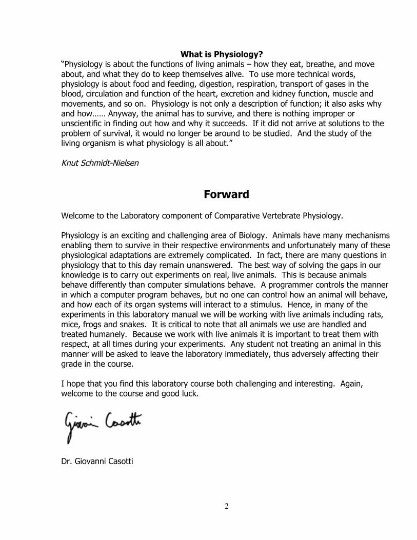
Forward Welcome to the Laboratory component of Comparative Vertebrate Physiology. Physiology is an exciting and challenging area of Biology. Animals have many mechanisms enabling them to survive in their respective environments and unfortunately many of these physiological adaptations are extremely complicated. In fact, there are many questions in physiology that to this day remain unanswered. The best way of solving the gaps in our knowledge is to carry out experiments on real, live animals. This is because animals behave differently than computer simulations behave. A programmer controls the manner in which a computer program behaves, but no one can control how an animal will behave, and how each of its organ systems will interact to a stimulus. Hence, in many of the experiments in this laboratory manual we will be working with live animals including rats, mice, frogs and snakes. It is critical to note that all animals we use are handled and treated humanely. Because we work with live animals it is important to treat them with respect, at all times during your experiments. Any student not treating an animal in this manner will be asked to leave the laboratory immediately, thus adversely affecting their grade in the course. I hope that you find this laboratory course both challenging and interesting. Again, welcome to the course and good luck.
Dr. Giovanni Casotti
3
Table of Contents Laboratory Timetable ............................................................................................................................ 4 The scientific method and an Introduction to PowerLab ............................................................. 5 How to write a scientific report ........................................................................................................................ 5 The Outline .............................................................................................................................................................. 5 The Report ............................................................................................................................................................... 6
Introduction to LabChart ...................................................................................................................... 10 Presenting Scientific Information ...................................................................................................... 25 Compound Action Potentials in the Frog Sciatic Nerve .............................................................. 26 Muscle Stimulation & Fatigue .............................................................................................................. 38 Hematology ................................................................................................................................................ 52 Cardiovascular Physiology ................................................................................................................... 59 Physiology of the in situ amphibian Heart ...................................................................................... 74 Respiration ................................................................................................................................................ 88 Osmoregulation ...................................................................................................................................... 108 Metabolism .............................................................................................................................................. 117 Digestion ................................................................................................................................................... 124 Group projects and oral presentations .......................................................................................... 127 Scoring Rubrics ...................................................................................................................................... 128
All experiments using PowerLab® are Copyright ADInstruments 2015.
Reprinted and modified with permission.
4
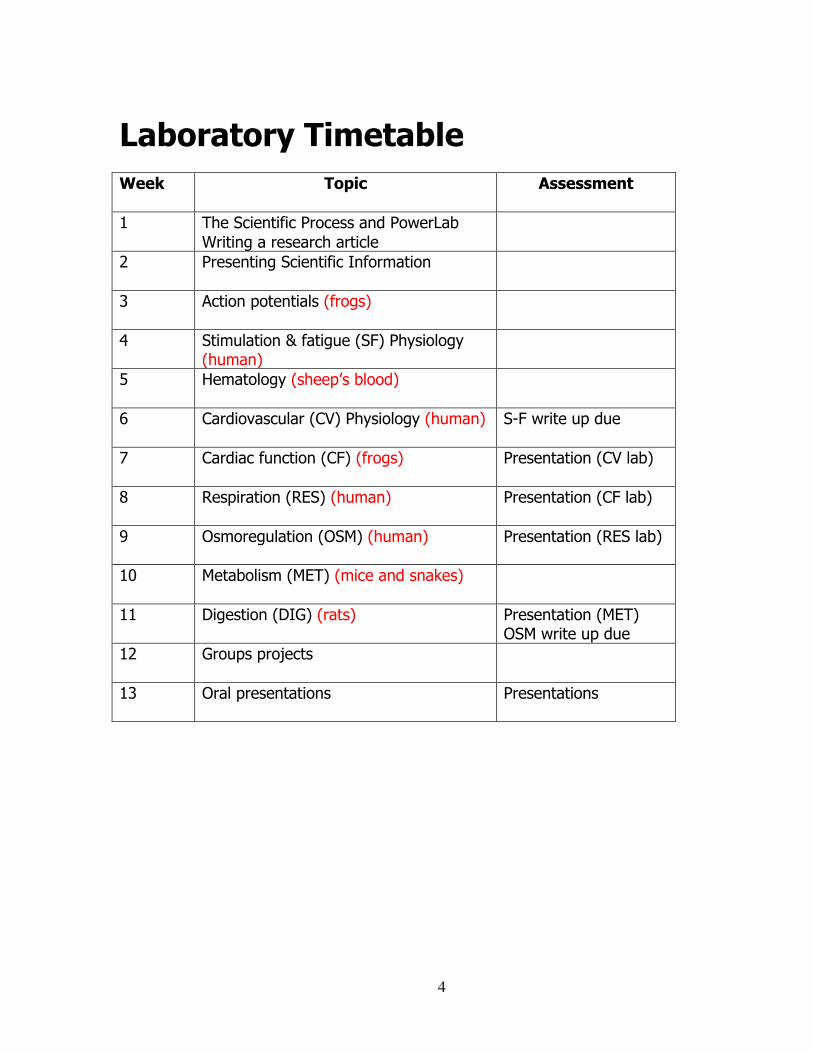
Laboratory Timetable Week Topic Assessment
1 The Scientific Process and PowerLab Writing a research article
2 Presenting Scientific Information
3 Action potentials (frogs)
4 Stimulation & fatigue (SF) Physiology (human)
5 Hematology (sheep’s blood)
6 Cardiovascular (CV) Physiology (human) S-F write up due
7 Cardiac function (CF) (frogs) Presentation (CV lab)
8 Respiration (RES) (human) Presentation (CF lab)
9 Osmoregulation (OSM) (human) Presentation (RES lab)
10 Metabolism (MET) (mice and snakes)
11 Digestion (DIG) (rats) Presentation (MET) OSM write up due
12 Groups projects
13 Oral presentations Presentations

5
The scientific method and an Introduction to PowerLab
Introduction The aims of this laboratory are to A. Familiarize yourself with the scientific method, B.
learn how to write an effective scientific report using a published paper as an example, C. complete a tutorial on how to use a data acquisition system called PowerLab.
Procedure A. The scientific method
The scientific method is not unfamiliar to you by now. The definition of the method is the approach commonly used by scientists when they investigate various aspects of their respective disciplines. Steps involved in the method are: Observation of phenomena, a statement of a hypothesis, data collection, data manipulation and analysis, and reporting conclusions of the study. B. Scientific report writing
Writing scientifically is not easy. For this course you need to write and hand in reports that will be used as part of your course grade. Below are guidelines on how to write a scientific report. Use these criteria, as I will be looking to make certain you follow these in your reports during the semester.
As part of the process on how to write a scientific report, we will go through a paper on Turtle navigation in class (J. Exp. Biol. 198: 1079-1085). This paper is at the end of this laboratory manual. Read the paper BEFORE class and identify AND prepare comments of the different areas of “The Report” (1 - 7) as listed below. We will go over them as a class during the laboratory.
How to write a scientific report Communicating your results with other members of the scientific community is as essential
as being a competent experimenter. The essence of a good report is a clear understanding of the aim, results and significance of
the experiment that have been translated into a written form. Even assuming that you have that understanding, very few of you will be able to put that down on paper in one attempt. In theory a draft copy that is completely edited and rewritten is needed to achieve the required degree of clarity. Indeed when writing for a journal one will go through many drafts before the final version is submitted to the editor.
The Outline
1. Style Scientific reports are generally written in past tense, and in first person narrative. For
example rather than writing: "In this experiment we will examine the effects of temperature on oxygen consumption .......", you should write: "In this experiment the effects of temperature on oxygen consumption were examined ........"
6
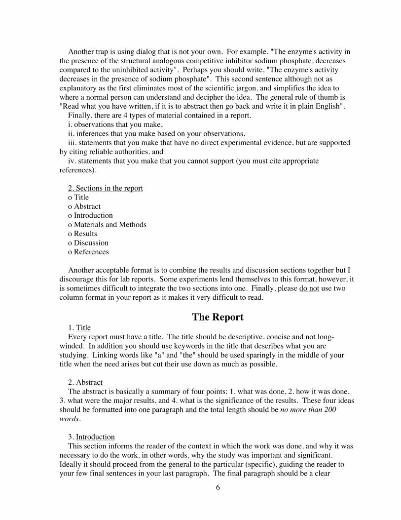
Another trap is using dialog that is not your own. For example, "The enzyme's activity in the presence of the structural analogous competitive inhibitor sodium phosphate, decreases compared to the uninhibited activity". Perhaps you should write, "The enzyme's activity decreases in the presence of sodium phosphate". This second sentence although not as explanatory as the first eliminates most of the scientific jargon, and simplifies the idea to where a normal person can understand and decipher the idea. The general rule of thumb is "Read what you have written, if it is to abstract then go back and write it in plain English".
Finally, there are 4 types of material contained in a report. i. observations that you make, ii. inferences that you make based on your observations, iii. statements that you make that have no direct experimental evidence, but are supported
by citing reliable authorities, and iv. statements that you make that you cannot support (you must cite appropriate
references). 2. Sections in the report o Title o Abstract o Introduction o Materials and Methods o Results o Discussion o References Another acceptable format is to combine the results and discussion sections together but I
discourage this for lab reports. Some experiments lend themselves to this format, however, it is sometimes difficult to integrate the two sections into one. Finally, please do not use two column format in your report as it makes it very difficult to read.
The Report
1. Title Every report must have a title. The title should be descriptive, concise and not long-
winded. In addition you should use keywords in the title that describes what you are studying. Linking words like "a" and "the" should be used sparingly in the middle of your title when the need arises but cut their use down as much as possible.
2. Abstract The abstract is basically a summary of four points: 1. what was done, 2. how it was done,
3. what were the major results, and 4. what is the significance of the results. These four ideas should be formatted into one paragraph and the total length should be no more than 200 words.
3. Introduction This section informs the reader of the context in which the work was done, and why it was
necessary to do the work, in other words, why the study was important and significant. Ideally it should proceed from the general to the particular (specific), guiding the reader to your few final sentences in your last paragraph. The final paragraph should be a clear
7
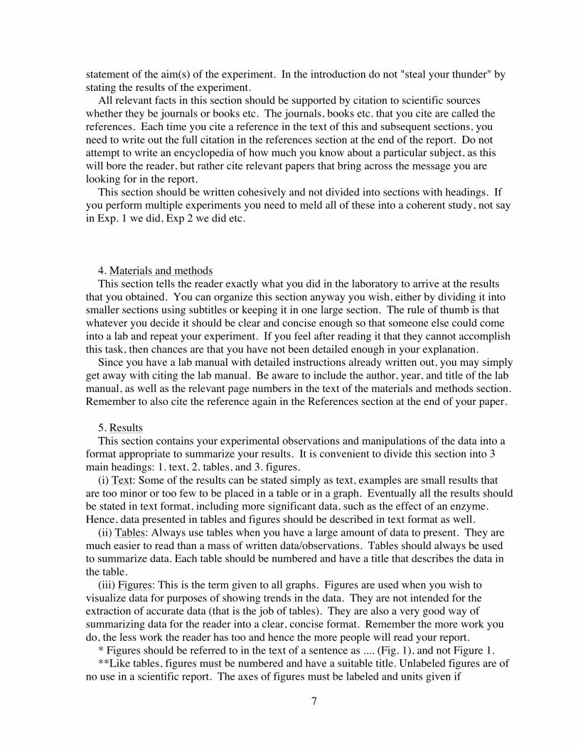
statement of the aim(s) of the experiment. In the introduction do not "steal your thunder" by stating the results of the experiment.
All relevant facts in this section should be supported by citation to scientific sources whether they be journals or books etc. The journals, books etc. that you cite are called the references. Each time you cite a reference in the text of this and subsequent sections, you need to write out the full citation in the references section at the end of the report. Do not attempt to write an encyclopedia of how much you know about a particular subject, as this will bore the reader, but rather cite relevant papers that bring across the message you are looking for in the report.
This section should be written cohesively and not divided into sections with headings. If you perform multiple experiments you need to meld all of these into a coherent study, not say in Exp. 1 we did, Exp 2 we did etc.
4. Materials and methods This section tells the reader exactly what you did in the laboratory to arrive at the results
that you obtained. You can organize this section anyway you wish, either by dividing it into smaller sections using subtitles or keeping it in one large section. The rule of thumb is that whatever you decide it should be clear and concise enough so that someone else could come into a lab and repeat your experiment. If you feel after reading it that they cannot accomplish this task, then chances are that you have not been detailed enough in your explanation.
Since you have a lab manual with detailed instructions already written out, you may simply get away with citing the lab manual. Be aware to include the author, year, and title of the lab manual, as well as the relevant page numbers in the text of the materials and methods section. Remember to also cite the reference again in the References section at the end of your paper.
5. Results This section contains your experimental observations and manipulations of the data into a
format appropriate to summarize your results. It is convenient to divide this section into 3 main headings: 1. text, 2. tables, and 3. figures.
(i) Text: Some of the results can be stated simply as text, examples are small results that are too minor or too few to be placed in a table or in a graph. Eventually all the results should be stated in text format, including more significant data, such as the effect of an enzyme. Hence, data presented in tables and figures should be described in text format as well.
(ii) Tables: Always use tables when you have a large amount of data to present. They are much easier to read than a mass of written data/observations. Tables should always be used to summarize data. Each table should be numbered and have a title that describes the data in the table.
(iii) Figures: This is the term given to all graphs. Figures are used when you wish to visualize data for purposes of showing trends in the data. They are not intended for the extraction of accurate data (that is the job of tables). They are also a very good way of summarizing data for the reader into a clear, concise format. Remember the more work you do, the less work the reader has too and hence the more people will read your report.
* Figures should be referred to in the text of a sentence as .... (Fig. 1), and not Figure 1. **Like tables, figures must be numbered and have a suitable title. Unlabeled figures are of
no use in a scientific report. The axes of figures must be labeled and units given if
8
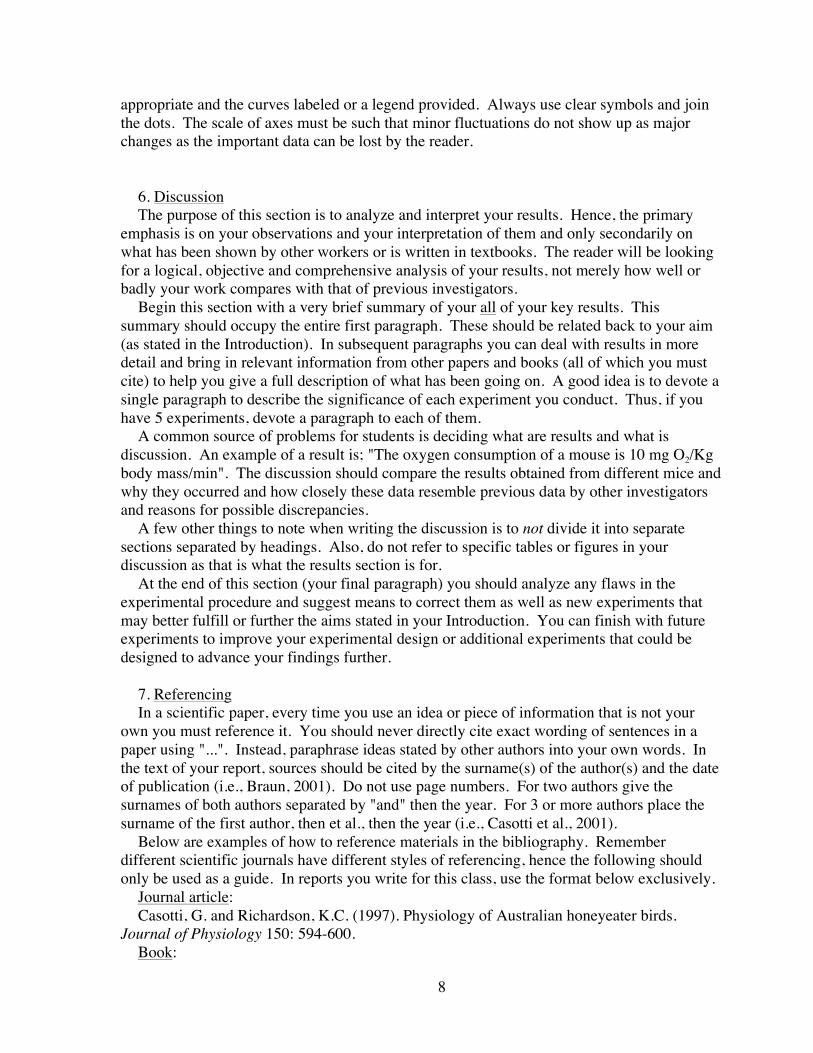
appropriate and the curves labeled or a legend provided. Always use clear symbols and join the dots. The scale of axes must be such that minor fluctuations do not show up as major changes as the important data can be lost by the reader.
6. Discussion The purpose of this section is to analyze and interpret your results. Hence, the primary
emphasis is on your observations and your interpretation of them and only secondarily on what has been shown by other workers or is written in textbooks. The reader will be looking for a logical, objective and comprehensive analysis of your results, not merely how well or badly your work compares with that of previous investigators.
Begin this section with a very brief summary of your all of your key results. This summary should occupy the entire first paragraph. These should be related back to your aim (as stated in the Introduction). In subsequent paragraphs you can deal with results in more detail and bring in relevant information from other papers and books (all of which you must cite) to help you give a full description of what has been going on. A good idea is to devote a single paragraph to describe the significance of each experiment you conduct. Thus, if you have 5 experiments, devote a paragraph to each of them.
A common source of problems for students is deciding what are results and what is discussion. An example of a result is; "The oxygen consumption of a mouse is 10 mg O2/Kg body mass/min". The discussion should compare the results obtained from different mice and why they occurred and how closely these data resemble previous data by other investigators and reasons for possible discrepancies.
A few other things to note when writing the discussion is to not divide it into separate sections separated by headings. Also, do not refer to specific tables or figures in your discussion as that is what the results section is for.
At the end of this section (your final paragraph) you should analyze any flaws in the experimental procedure and suggest means to correct them as well as new experiments that may better fulfill or further the aims stated in your Introduction. You can finish with future experiments to improve your experimental design or additional experiments that could be designed to advance your findings further.
7. Referencing In a scientific paper, every time you use an idea or piece of information that is not your
own you must reference it. You should never directly cite exact wording of sentences in a paper using "...". Instead, paraphrase ideas stated by other authors into your own words. In the text of your report, sources should be cited by the surname(s) of the author(s) and the date of publication (i.e., Braun, 2001). Do not use page numbers. For two authors give the surnames of both authors separated by "and" then the year. For 3 or more authors place the surname of the first author, then et al., then the year (i.e., Casotti et al., 2001).
Below are examples of how to reference materials in the bibliography. Remember different scientific journals have different styles of referencing, hence the following should only be used as a guide. In reports you write for this class, use the format below exclusively.
Journal article: Casotti, G. and Richardson, K.C. (1997). Physiology of Australian honeyeater birds.
Journal of Physiology 150: 594-600. Book:

9
Casotti, G. and Richardson, K.C. (1997). Physiology of Australian honeyeaters. MacMillan Publishing Company, New York.
Book Chapter: Casotti, G. and Richardson, K.C. (1997). Physiology of Australian honeyeater birds. In:
Avian Physiology and Anatomy. Arena, P.A. (Ed.). MacMillan Publishing Company, New York. p. 563-602.
Finally Once you have completed all the above you should correct your report for spelling and
grammatical errors. A good idea is to read the entire paper out aloud to yourself. In this day and age of spelling and grammar checkers there is no excuse for incorrect spelling or poor grammar. Good luck.
10
Introduction to LabChart In this experiment, you will learn how to acquire data with the PowerLab Data Acquisition Unit and analyze the data using the LabChart software. You will make simple recordings and measurements using the Finger Pulse Transducer.
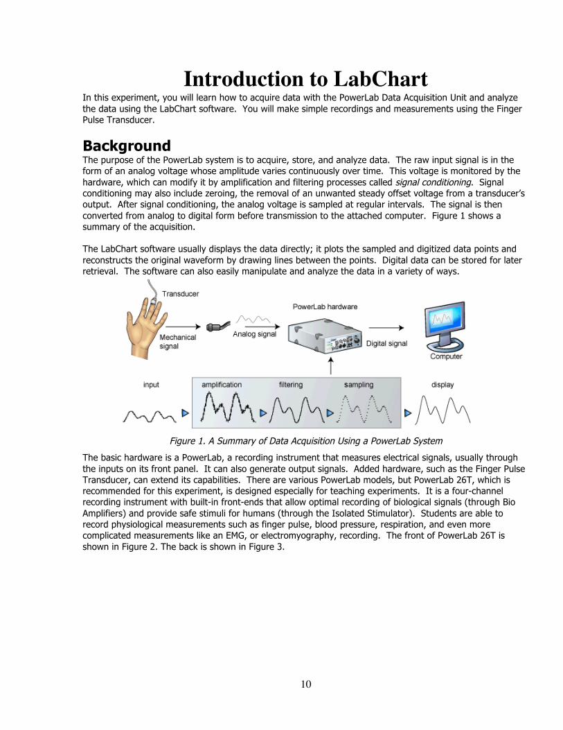
Background The purpose of the PowerLab system is to acquire, store, and analyze data. The raw input signal is in the form of an analog voltage whose amplitude varies continuously over time. This voltage is monitored by the hardware, which can modify it by amplification and filtering processes called signal conditioning. Signal conditioning may also include zeroing, the removal of an unwanted steady offset voltage from a transducer’s output. After signal conditioning, the analog voltage is sampled at regular intervals. The signal is then converted from analog to digital form before transmission to the attached computer. Figure 1 shows a summary of the acquisition. The LabChart software usually displays the data directly; it plots the sampled and digitized data points and reconstructs the original waveform by drawing lines between the points. Digital data can be stored for later retrieval. The software can also easily manipulate and analyze the data in a variety of ways.
Figure 1. A Summary of Data Acquisition Using a PowerLab System
The basic hardware is a PowerLab, a recording instrument that measures electrical signals, usually through the inputs on its front panel. It can also generate output signals. Added hardware, such as the Finger Pulse Transducer, can extend its capabilities. There are various PowerLab models, but PowerLab 26T, which is recommended for this experiment, is designed especially for teaching experiments. It is a four-channel recording instrument with built-in front-ends that allow optimal recording of biological signals (through Bio Amplifiers) and provide safe stimuli for humans (through the Isolated Stimulator). Students are able to record physiological measurements such as finger pulse, blood pressure, respiration, and even more complicated measurements like an EMG, or electromyography, recording. The front of PowerLab 26T is shown in Figure 2. The back is shown in Figure 3.
11
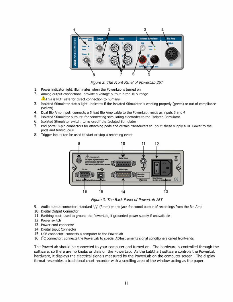
Figure 2. The Front Panel of PowerLab 26T
1. Power indicator light: illuminates when the PowerLab is turned on 2. Analog output connections: provide a voltage output in the 10 V range
This is NOT safe for direct connection to humans 3. Isolated Stimulator status light: indicates if the Isolated Stimulator is working properly (green) or out of compliance
(yellow) 4. Dual Bio Amp input: connects a 5 lead Bio Amp cable to the PowerLab; reads as inputs 3 and 4 5. Isolated Stimulator outputs: for connecting stimulating electrodes to the Isolated Stimulator 6. Isolated Stimulator switch: turns on/off the Isolated Stimulator 7. Pod ports: 8-pin connectors for attaching pods and certain transducers to Input; these supply a DC Power to the
pods and transducers 8. Trigger input: can be used to start or stop a recording event
Figure 3. The Back Panel of PowerLab 26T
9. Audio output connector: standard 1/8'' (3mm) phono jack for sound output of recordings from the Bio Amp 10. Digital Output Connector 11. Earthing post: used to ground the PowerLab, if grounded power supply if unavailable 12. Power switch 13. Power cord connector 14. Digital Input Connector 15. USB connector: connects a computer to the PowerLab 16. I2C connector: connects the PowerLab to special ADInstruments signal conditioners called front-ends The PowerLab should be connected to your computer and turned on. The hardware is controlled through the software, so there are no knobs or dials on the PowerLab. As the LabChart software controls the PowerLab hardware, it displays the electrical signals measured by the PowerLab on the computer screen. The display format resembles a traditional chart recorder with a scrolling area of the window acting as the paper.
12
Required Equipment • LabChart software • PowerLab Data Acquisition Unit • Finger Pulse Transducer
Procedure Words appearing in bold are items to click in LabChart. If the word appears in bold and a color, it is referred to in the Student Quick Reference Guide. Use the color dividers in the guide to find the appropriate section for your topic. All blue text appears in Part One: Acquisition, all green text appears in Part Two: Data Analysis, and all red text appears in Part Three: Troubleshooting. An introduction to the PowerLab and LabChart appears in the purple section.
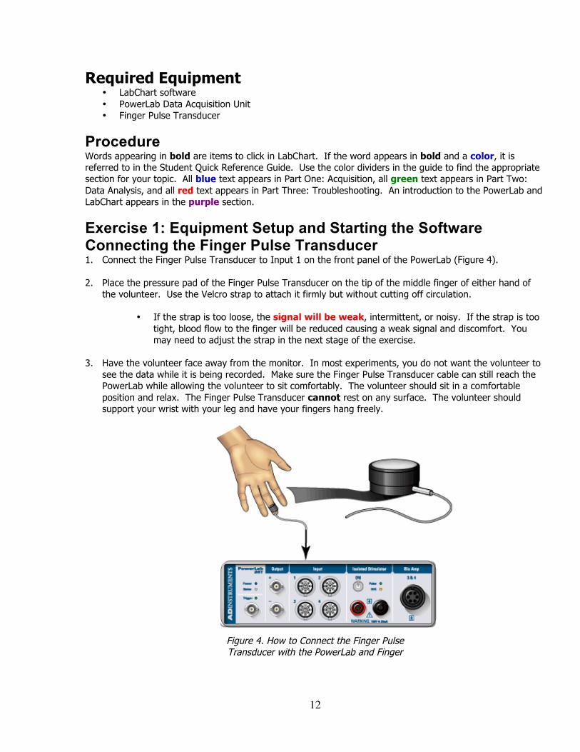
Exercise 1: Equipment Setup and Starting the Software Connecting the Finger Pulse Transducer 1. Connect the Finger Pulse Transducer to Input 1 on the front panel of the PowerLab (Figure 4). 2. Place the pressure pad of the Finger Pulse Transducer on the tip of the middle finger of either hand of
the volunteer. Use the Velcro strap to attach it firmly but without cutting off circulation.
• If the strap is too loose, the signal will be weak, intermittent, or noisy. If the strap is too tight, blood flow to the finger will be reduced causing a weak signal and discomfort. You may need to adjust the strap in the next stage of the exercise.
3. Have the volunteer face away from the monitor. In most experiments, you do not want the volunteer to
see the data while it is being recorded. Make sure the Finger Pulse Transducer cable can still reach the PowerLab while allowing the volunteer to sit comfortably. The volunteer should sit in a comfortable position and relax. The Finger Pulse Transducer cannot rest on any surface. The volunteer should support your wrist with your leg and have your fingers hang freely.
Figure 4. How to Connect the Finger Pulse Transducer with the PowerLab and Finger
13
Starting the LabChart Software 1. Start the LabChart software as you would any other computer program. LabChart will appear with either
an empty Chart Window (Figure 5) or the Experiments Gallery dialog. If the Welcome Center appears, close it to see the Chart Window.
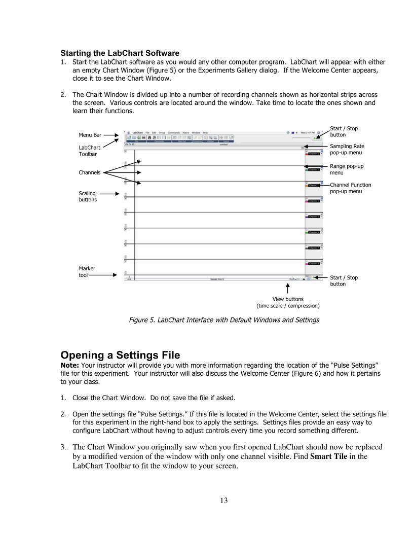
2. The Chart Window is divided up into a number of recording channels shown as horizontal strips across
the screen. Various controls are located around the window. Take time to locate the ones shown and learn their functions.
Figure 5. LabChart Interface with Default Windows and Settings
Opening a Settings File Note: Your instructor will provide you with more information regarding the location of the “Pulse Settings” file for this experiment. Your instructor will also discuss the Welcome Center (Figure 6) and how it pertains to your class. 1. Close the Chart Window. Do not save the file if asked.
2. Open the settings file “Pulse Settings.” If this file is located in the Welcome Center, select the settings file
for this experiment in the right-hand box to apply the settings. Settings files provide an easy way to configure LabChart without having to adjust controls every time you record something different.
3. The Chart Window you originally saw when you first opened LabChart should now be replaced
by a modified version of the window with only one channel visible. Find Smart Tile in the LabChart Toolbar to fit the window to your screen.
Menu Bar
LabChart Toolbar
Sampling Rate pop-up menu
Channels
Scaling buttons
Marker tool
Range pop-up menu
Channel Function pop-up menu
Start / Stop button
Start / Stop button
View buttons (time scale / compression)
14
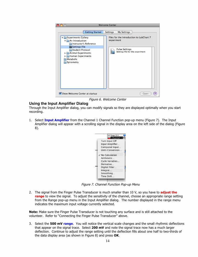
Figure 6. Welcome Center
Using the Input Amplifier Dialog Through the Input Amplifier dialog, you can modify signals so they are displayed optimally when you start recording. 1. Select Input Amplifier from the Channel 1 Channel Function pop-up menu (Figure 7). The Input
Amplifier dialog will appear with a scrolling signal in the display area on the left side of the dialog (Figure 8).
Figure 7. Channel Function Pop-up Menu
2. The signal from the Finger Pulse Transducer is much smaller than 10 V, so you have to adjust the
range to view the signal. To adjust the sensitivity of the channel, choose an appropriate range setting from the Range pop-up menu in the Input Amplifier dialog. The number displayed in the range menu indicates the maximum input voltage currently selected.
Note: Make sure the Finger Pulse Transducer is not touching any surface and is still attached to the volunteer. Refer to “Connecting the Finger Pulse Transducer” above. 3. Select the 500 mV range. You will notice the vertical scale changes and the small rhythmic deflections
that appear on the signal trace. Select 200 mV and note the signal trace now has a much larger deflection. Continue to adjust the range setting until the deflection fills about one half to two-thirds of the data display area (as shown in Figure 8) and press OK.

15
4. The signal from the Finger Pulse Transducer has not changed, only the sensitivity of the recording
system has. If the rhythmic signal is a series of downward deflections, click in the Invert checkbox to reverse the direction.
Figure 8. Input Amplifier Dialog
Creating Digital Voltmeter Mini-windows (DVMs) It is possible to create mini-windows of the Rate/Time and Range/Amplitude. This allows you to see the numbers clearly if you are recording data away from the monitor. 3. Position the cursor over the Rate/Time. Click-and-drag this area to create the DVM. You can
then do the same for Range. Figure 9 shows where to position the cursor. Once created, you can move the DVMs anywhere on the screen.
• When the cursor in is the data channels, the DVMs will display the time and amplitude. When the cursor is elsewhere in the window, the DVMs will be blank. An example of these DVMs is shown in Figure 10.
Figure 9. The Circles Indicate Where to Figure 10. DVMs Position the Cursor to Create DVMs Saving the File It is wise to save work frequently when working with any computer. Saving files in LabChart is the same as saving any file you would on your personal computer. If you choose to save your files, the Save As dialog will appear so you can save the file under a suitable name and location.
16
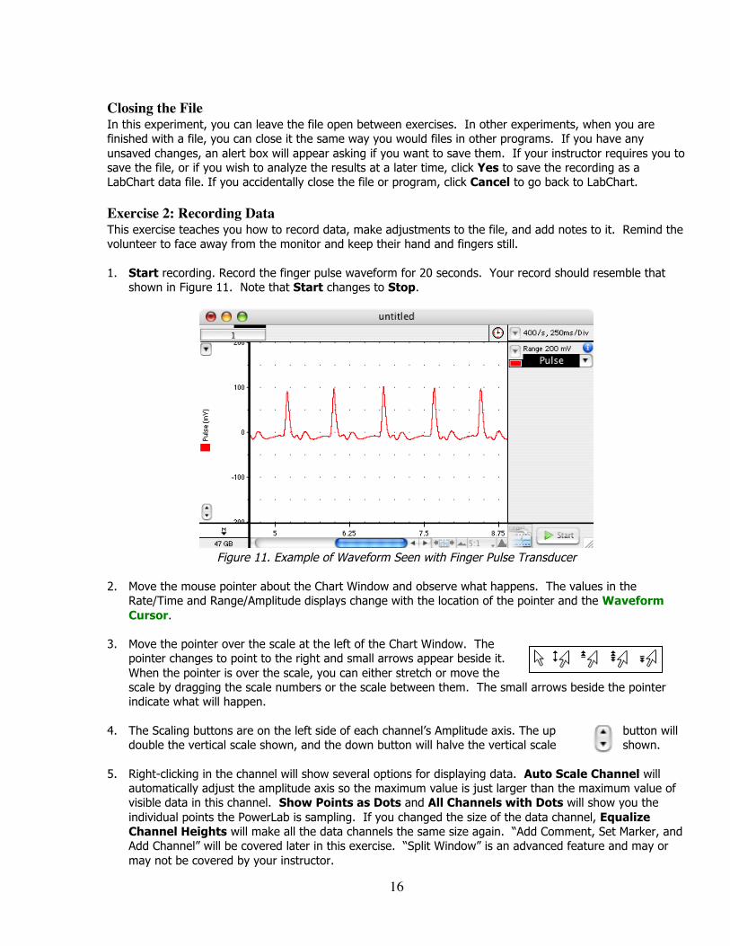
Closing the File In this experiment, you can leave the file open between exercises. In other experiments, when you are finished with a file, you can close it the same way you would files in other programs. If you have any unsaved changes, an alert box will appear asking if you want to save them. If your instructor requires you to save the file, or if you wish to analyze the results at a later time, click Yes to save the recording as a LabChart data file. If you accidentally close the file or program, click Cancel to go back to LabChart. Exercise 2: Recording Data This exercise teaches you how to record data, make adjustments to the file, and add notes to it. Remind the volunteer to face away from the monitor and keep their hand and fingers still. 1. Start recording. Record the finger pulse waveform for 20 seconds. Your record should resemble that
shown in Figure 11. Note that Start changes to Stop.
Figure 11. Example of Waveform Seen with Finger Pulse Transducer
2. Move the mouse pointer about the Chart Window and observe what happens. The values in the
Rate/Time and Range/Amplitude displays change with the location of the pointer and the Waveform Cursor.
3. Move the pointer over the scale at the left of the Chart Window. The
pointer changes to point to the right and small arrows appear beside it. When the pointer is over the scale, you can either stretch or move the scale by dragging the scale numbers or the scale between them. The small arrows beside the pointer indicate what will happen.
4. The Scaling buttons are on the left side of each channel’s Amplitude axis. The up button will
double the vertical scale shown, and the down button will halve the vertical scale shown. 5. Right-clicking in the channel will show several options for displaying data. Auto Scale Channel will
automatically adjust the amplitude axis so the maximum value is just larger than the maximum value of visible data in this channel. Show Points as Dots and All Channels with Dots will show you the individual points the PowerLab is sampling. If you changed the size of the data channel, Equalize Channel Heights will make all the data channels the same size again. “Add Comment, Set Marker, and Add Channel” will be covered later in this exercise. “Split Window” is an advanced feature and may or may not be covered by your instructor.
17
Note: AutoScale is also found in the LabChart Toolbar under the Command Auto Scale All Channels. Adjusting the Sampling Rate Look at your data trace in the Chart Window. The peaks may not look quite the same as they did in the Input Amplifier dialog. This can be explained in terms of sampling rate. A digital recording system, like the PowerLab system, records the value of the signal at regular time intervals, rather than continuously. This is called sampling. When sampling occurs too slowly, some of the faster parts of the waveform, like the pulse peak, may not be recorded causing the recorded signal to inaccurately represent the real one. To record a signal accurately using this technique, the sampling rate must be set high enough that the signal does not vary too much between samples.
You will be running a macro to adjust the sampling rate.
Running Macros A macro is a recorded set of commands and operations which can be executed with a single command. If you want settings to change while you are recording, you can create a macro to automatically change the settings for you at a specific time. The settings file you opened for this experiment contains one macro to automatically adjust the sampling rate for you. Macros are used in many other LabChart experiments. 1. Select Macro from the Menu Bar and scroll down to “Sampling Rate.” This is the title of the macro.
Have the volunteer relax and wear the Finger Pulse Transducer as before. The macro will do everything for you – it will even stop recording.
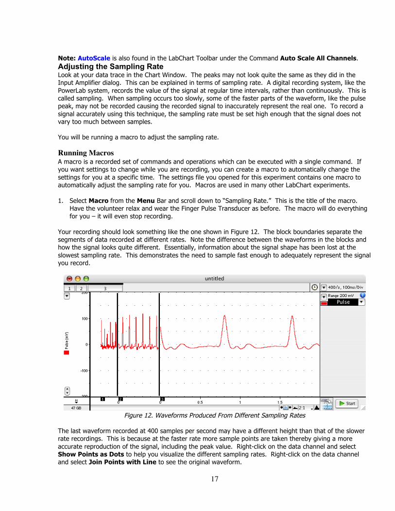
Your recording should look something like the one shown in Figure 12. The block boundaries separate the segments of data recorded at different rates. Note the difference between the waveforms in the blocks and how the signal looks quite different. Essentially, information about the signal shape has been lost at the slowest sampling rate. This demonstrates the need to sample fast enough to adequately represent the signal you record.
Figure 12. Waveforms Produced From Different Sampling Rates
The last waveform recorded at 400 samples per second may have a different height than that of the slower rate recordings. This is because at the faster rate more sample points are taken thereby giving a more accurate reproduction of the signal, including the peak value. Right-click on the data channel and select Show Points as Dots to help you visualize the different sampling rates. Right-click on the data channel and select Join Points with Line to see the original waveform.
18
Annotating a Record This experiment is divided into a series of exercises. It is convenient to annotate each exercise, using a comment, to determine what was done at any particular stage during subsequent review. In many experiments, adding comments will be part of the procedure. You can add comments while you are still recording and after you have finished.
1. Set the sampling rate to 400 samples per second (400/s) and Start recording.
2. Type “comment 1” or something similar on the keyboard. The words appear in the Comments bar at the bottom of the Chart Window. Add the comment by pressing Return/Enter or by Add at the right of the Comments bar.
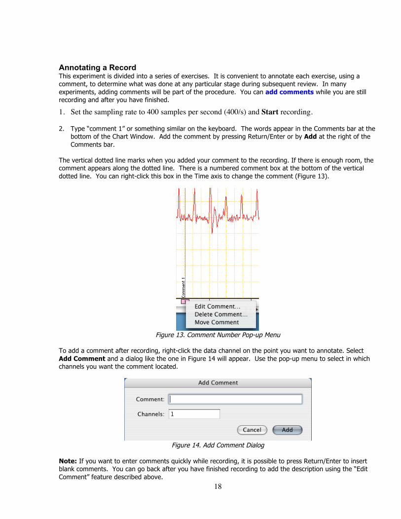
The vertical dotted line marks when you added your comment to the recording. If there is enough room, the comment appears along the dotted line. There is a numbered comment box at the bottom of the vertical dotted line. You can right-click this box in the Time axis to change the comment (Figure 13).
Figure 13. Comment Number Pop-up Menu
To add a comment after recording, right-click the data channel on the point you want to annotate. Select Add Comment and a dialog like the one in Figure 14 will appear. Use the pop-up menu to select in which channels you want the comment located.
Figure 14. Add Comment Dialog
Note: If you want to enter comments quickly while recording, it is possible to press Return/Enter to insert blank comments. You can go back after you have finished recording to add the description using the “Edit Comment” feature described above.
19
Exercise 3: Analysis The LabChart program is not only used to record waveforms but also to analyze them. This exercise shows you how to use more features of LabChart: navigating the Chart Window to find data, measuring amplitude and time values from the waveform, using the Zoom Window for a more detailed view, and creating channel calculations. Navigating in the Chart Window There are a variety of ways to view a LabChart data file and to navigate around it. You can use the scroll bar to scroll to different parts of the recording, compress the Time axis so more of a waveform can be seen, and locate specific sections of the recording by searching for the comment inserted there. Scrolling The scroll bar provides the simplest way of moving backwards and forwards through your file and works the same as it would in any other computer program. You can think of your recording as a large strip of paper of which only one part can be seen at any one time. Note: If your mouse is equipped with a scroll wheel, rolling the wheel forward will scroll your data to the right and rolling the wheel to the rear will scroll to the left.
View Buttons By using the View Buttons at the bottom of the Chart Window, you can compress or expand the Time axis to see more or less of a waveform. The left button will compress your data. The right button will expand it. If you select the ration button, a pop-up menu appears in which you can choose the new compression directly.
Locating Specific Sections by Comments The Commands menu has some other ways you can navigate around your recording. Find brings up the “Find and Select” dialog. Each type of find is based on an initial selection or active point, which serves as a starting point for the find. Find Next will perform the find a second time in the direction chosen in the Find and Select dialog. Go to Start will take you to the beginning of the Data file. Go to End will take you to the end of the data file. 1. Select Find in the LabChart Toolbar and go to Find Comment. Choose the search direction and
enter text from the comment you wish to find. (If the comment is already in the Chart Window, the data trace will not move.)
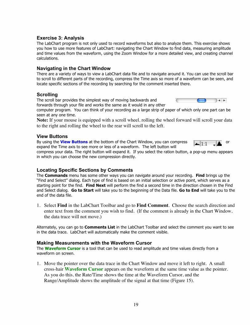
Alternately, you can go to Comments List in the LabChart Toolbar and select the comment you want to see in the data trace. LabChart will automatically make the comment visible. Making Measurements with the Waveform Cursor The Waveform Cursor is a tool that can be used to read amplitude and time values directly from a waveform on screen. 1. Move the pointer over the data trace in the Chart Window and move it left to right. A small
cross-hair Waveform Cursor appears on the waveform at the same time value as the pointer. As you do this, the Rate/Time shows the time at the Waveform Cursor, and the Range/Amplitude shows the amplitude of the signal at that time (Figure 15).
20
Figure 15. Waveform Cursor and Pointer
Using the Marker The Waveform Cursor is often used in conjunction with the Marker. The Marker is located at the bottom left of the Chart Window and can be dropped on any part of the waveform to allow relative measurements.
1. Drag the Marker from the Marker Box to a location on the trace and release. The Marker does not have to be placed exactly on the waveform; it will attach itself to the waveform at the time position you dropped it.
2. Move the pointer away from the Marker. When the Marker is in use, the amplitude and time values
displayed are relative to the marked reference point. This means the time and amplitude values are now displayed as differences (∆) between the Waveform Cursor and the Marker. This is very useful for measuring the time between events or measuring the relative amplitudes of parts of a waveform.
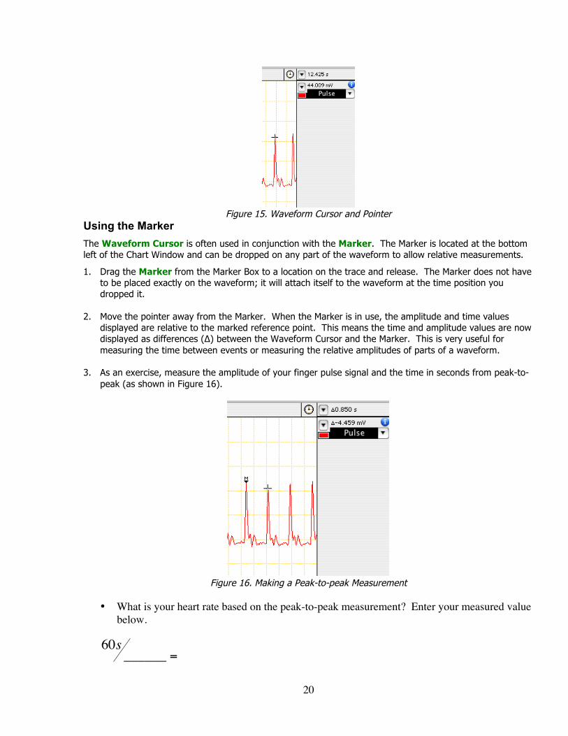
3. As an exercise, measure the amplitude of your finger pulse signal and the time in seconds from peak-to-
peak (as shown in Figure 16).
Figure 16. Making a Peak-to-peak Measurement
• What is your heart rate based on the peak-to-peak measurement? Enter your measured value
below.
!
60s______ =
21
The heart rate calculated from the time difference shown in Figure 16 would be 60 s / 0.850 s = 70.59 beats per minute (BPM). If you want to remove the Marker from the data trace, either click in the Marker Box to return the Marker home or drag the Marker back to its home location. Using the Zoom Window A convenient feature of LabChart is the ability to zoom in on a selected region of data. This allows you to select a specific area of a signal and look at it much more closely. It also allows accurate measurements to be made more easily. With Zoom Window, you can copy the image onto the Clipboard so it can be pasted into a word-processor or graphics file. (The Copy command from the Edit menu changes to Copy Zoom Window when the Zoom Window is in front.) You can print the image on a connected printer.
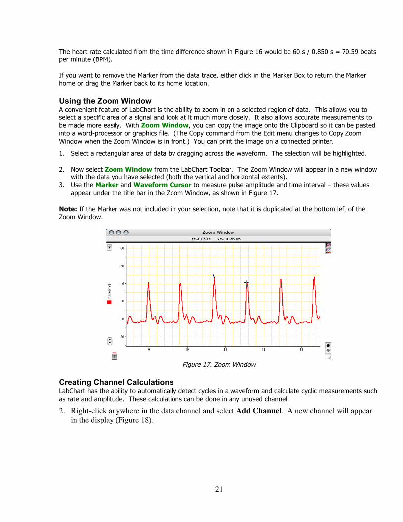
1. Select a rectangular area of data by dragging across the waveform. The selection will be highlighted. 2. Now select Zoom Window from the LabChart Toolbar. The Zoom Window will appear in a new window
with the data you have selected (both the vertical and horizontal extents). 3. Use the Marker and Waveform Cursor to measure pulse amplitude and time interval – these values
appear under the title bar in the Zoom Window, as shown in Figure 17. Note: If the Marker was not included in your selection, note that it is duplicated at the bottom left of the Zoom Window.
Figure 17. Zoom Window
Creating Channel Calculations LabChart has the ability to automatically detect cycles in a waveform and calculate cyclic measurements such as rate and amplitude. These calculations can be done in any unused channel.
2. Right-click anywhere in the data channel and select Add Channel. A new channel will appear in the display (Figure 18).
22
Figure 18. Chart Window with Two Channels
3. From the Channel 2 Channel Function pop-up menu, select Cyclic Measurements.
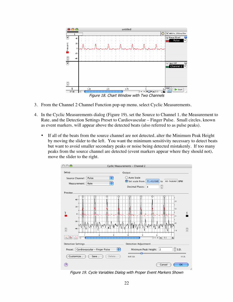
4. In the Cyclic Measurements dialog (Figure 19), set the Source to Channel 1, the Measurement to Rate, and the Detection Settings Preset to Cardiovascular – Finger Pulse. Small circles, known as event markers, will appear above the detected beats (also referred to as pulse peaks).
• If all of the beats from the source channel are not detected, alter the Minimum Peak Height by moving the slider to the left. You want the minimum sensitivity necessary to detect beats but want to avoid smaller secondary peaks or noise being detected mistakenly. If too many peaks from the source channel are detected (event markers appear where they should not), move the slider to the right.
Figure 19. Cycle Variables Dialog with Proper Event Markers Shown
23
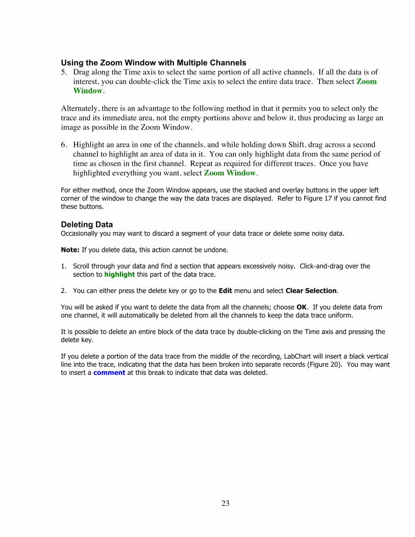
Using the Zoom Window with Multiple Channels 5. Drag along the Time axis to select the same portion of all active channels. If all the data is of
interest, you can double-click the Time axis to select the entire data trace. Then select Zoom Window.
Alternately, there is an advantage to the following method in that it permits you to select only the trace and its immediate area, not the empty portions above and below it, thus producing as large an image as possible in the Zoom Window.
6. Highlight an area in one of the channels, and while holding down Shift, drag across a second channel to highlight an area of data in it. You can only highlight data from the same period of time as chosen in the first channel. Repeat as required for different traces. Once you have highlighted everything you want, select Zoom Window.
For either method, once the Zoom Window appears, use the stacked and overlay buttons in the upper left corner of the window to change the way the data traces are displayed. Refer to Figure 17 if you cannot find these buttons. Deleting Data Occasionally you may want to discard a segment of your data trace or delete some noisy data. Note: If you delete data, this action cannot be undone. 1. Scroll through your data and find a section that appears excessively noisy. Click-and-drag over the
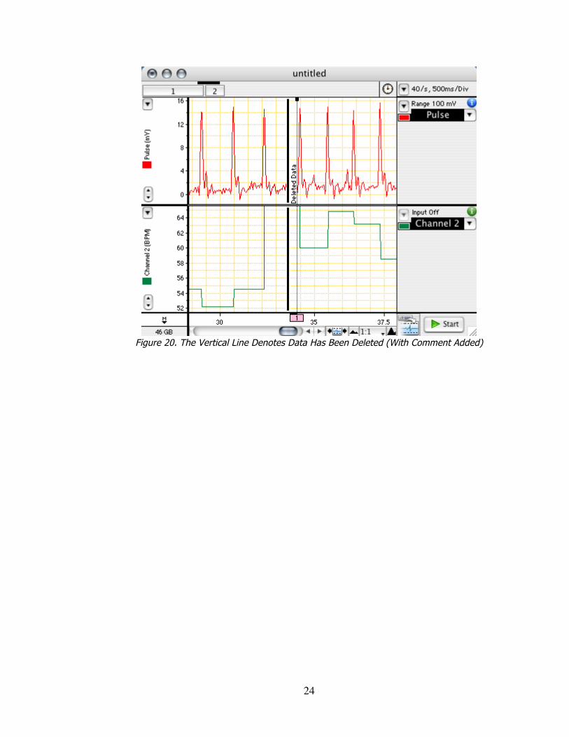
section to highlight this part of the data trace. 2. You can either press the delete key or go to the Edit menu and select Clear Selection. You will be asked if you want to delete the data from all the channels; choose OK. If you delete data from one channel, it will automatically be deleted from all the channels to keep the data trace uniform. It is possible to delete an entire block of the data trace by double-clicking on the Time axis and pressing the delete key. If you delete a portion of the data trace from the middle of the recording, LabChart will insert a black vertical line into the trace, indicating that the data has been broken into separate records (Figure 20). You may want to insert a comment at this break to indicate that data was deleted.
24
Figure 20. The Vertical Line Denotes Data Has Been Deleted (With Comment Added)

25
Presenting Scientific Information
In this laboratory I will present ways in which scientists disseminate information. Use the information from today’s class as a template on how to present scientific data. This information will be of use to you to help guide you in preparing and practicing your oral presentations in the final week of lab. The PowerPoint slides I will use for today’s class will be available for download on the web at the URL: http://darwin.wcupa.edu/faculty/casotti/Main/468lab. Once at this link, go to laboratories and download the PowerPoint slides.
Once the presentation is over we will go through the paper on Turtle navigation as a class (J. Exp. Biol. 198: 1079-1085). This paper is available online on the lab website. Read the paper BEFORE class and identify AND prepare comments of the different areas of “The Report” (1 - 7) pages 5 – 8 of this manual. Be prepared to provide your opinions to the rest of the class.
26
Compound Action Potentials in the Frog Sciatic Nerve
Background The fundamental unit of the nervous system is the neuron. Neurons and other excitable
cells produce action potentials when they receive electrical or chemical stimulation. The action potential occurs as a large-scale depolarization when positive ions such as sodium rapidly enter the neuron via specialized membrane channel proteins. Action potentials are “all-or-none” events. Once an action potential begins, it propagates down the length of the axon. When the action potential reaches the end of the axon, a neurotransmitter is typically released into the synapse. After an action potential occurs, the neuron must repolarize. During this time, called the refractory period, the neuron is incapable of producing another action potential. Measuring action potentials from single neurons requires highly specialized equipment. In this lab, you will record compound action potentials (CAP’s) from the isolated frog sciatic nerve. CAP’s represent the summed action potentials of the multitude of neurons that comprise a nerve. Required Equipment A computer system PowerLab with analog output LabChart software MLT012/B Nerve Bath Frog Ringer’s solution
Isolated frog sciatic nerve Dissection kit Glass needles Centimeter ruler Filter paper Suture
Procedures Setup and calibration of equipment
1. Connect the red and black alligator clips from the stimulator electrodes to two of the metal rungs on opposite sides of the MLT012/B Nerve Bath (Fig. 1). The distance between the electrodes should be 0.5 cm. It is not necessary to connect the green (ground) alligator clip. 2. Connect the red (positive) BNC connector from the stimulator electrode to the positive (+) analog output connector on the PowerLab. Connect the black (negative) BNC connector from the stimulator electrode to the negative (–) analog output connector.
3. Connect the red and black leads from the first recording electrode to two of the metal rungs of the MLT012/B Nerve Bath (Fig. 2). Connect the 8-pin pod connector to the Pod port on Input 1 of the PowerLab. 4. Repeat step 3 for the second recording electrode, only place the alligator clips further away from the stimulus electrode (Fig. 3). Attach the pod connector to the Pod port on Input 2 on the PowerLab.
27
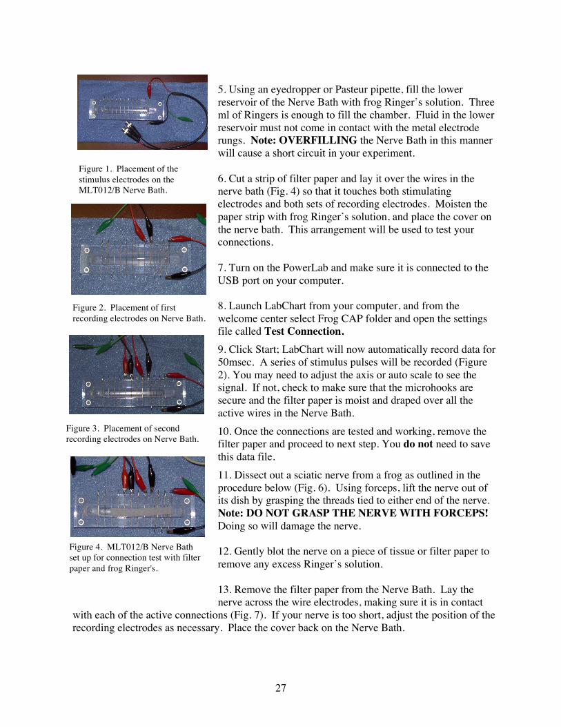
5. Using an eyedropper or Pasteur pipette, fill the lower reservoir of the Nerve Bath with frog Ringer’s solution. Three ml of Ringers is enough to fill the chamber. Fluid in the lower reservoir must not come in contact with the metal electrode rungs. Note: OVERFILLING the Nerve Bath in this manner will cause a short circuit in your experiment. 6. Cut a strip of filter paper and lay it over the wires in the nerve bath (Fig. 4) so that it touches both stimulating electrodes and both sets of recording electrodes. Moisten the paper strip with frog Ringer’s solution, and place the cover on the nerve bath. This arrangement will be used to test your connections. 7. Turn on the PowerLab and make sure it is connected to the USB port on your computer. 8. Launch LabChart from your computer, and from the welcome center select Frog CAP folder and open the settings file called Test Connection. 9. Click Start; LabChart will now automatically record data for 50msec. A series of stimulus pulses will be recorded (Figure 2). You may need to adjust the axis or auto scale to see the signal. If not, check to make sure that the microhooks are secure and the filter paper is moist and draped over all the active wires in the Nerve Bath. 10. Once the connections are tested and working, remove the filter paper and proceed to next step. You do not need to save this data file. 11. Dissect out a sciatic nerve from a frog as outlined in the procedure below (Fig. 6). Using forceps, lift the nerve out of its dish by grasping the threads tied to either end of the nerve. Note: DO NOT GRASP THE NERVE WITH FORCEPS! Doing so will damage the nerve. 12. Gently blot the nerve on a piece of tissue or filter paper to remove any excess Ringer’s solution. 13. Remove the filter paper from the Nerve Bath. Lay the nerve across the wire electrodes, making sure it is in contact
with each of the active connections (Fig. 7). If your nerve is too short, adjust the position of the recording electrodes as necessary. Place the cover back on the Nerve Bath.
Figure 4. MLT012/B Nerve Bath set up for connection test with filter paper and frog Ringer's.
Figure 3. Placement of second recording electrodes on Nerve Bath.
Figure 1. Placement of the stimulus electrodes on the MLT012/B Nerve Bath.
Figure 2. Placement of first recording electrodes on Nerve Bath.
28
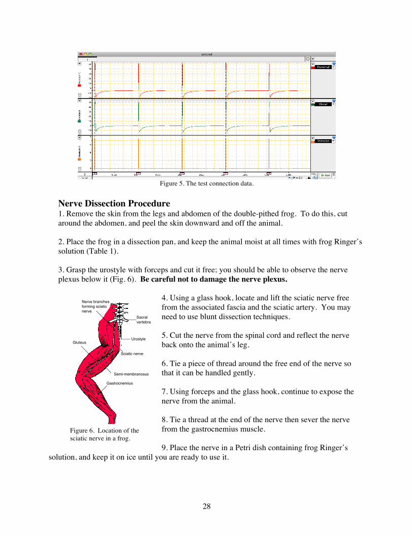
Figure 5. The test connection data.
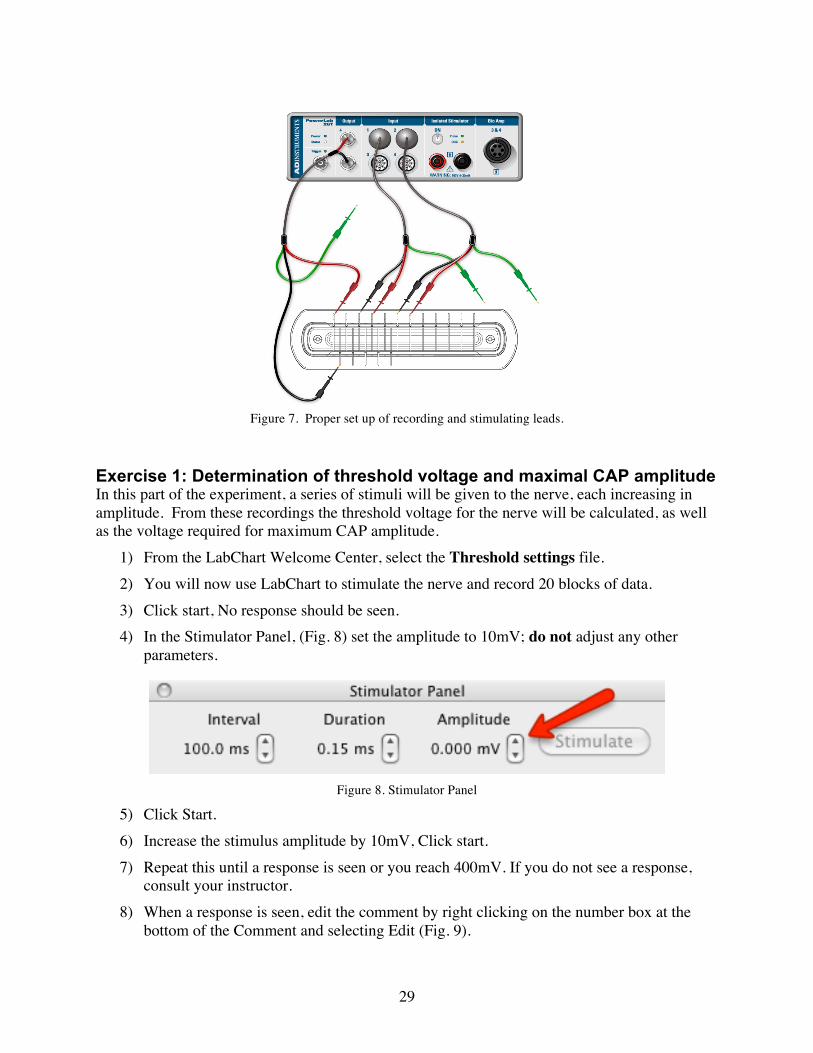
Nerve Dissection Procedure 1. Remove the skin from the legs and abdomen of the double-pithed frog. To do this, cut around the abdomen, and peel the skin downward and off the animal.
2. Place the frog in a dissection pan, and keep the animal moist at all times with frog Ringer’s solution (Table 1).
3. Grasp the urostyle with forceps and cut it free; you should be able to observe the nerve plexus below it (Fig. 6). Be careful not to damage the nerve plexus.
4. Using a glass hook, locate and lift the sciatic nerve free from the associated fascia and the sciatic artery. You may need to use blunt dissection techniques. 5. Cut the nerve from the spinal cord and reflect the nerve back onto the animal’s leg. 6. Tie a piece of thread around the free end of the nerve so that it can be handled gently. 7. Using forceps and the glass hook, continue to expose the nerve from the animal. 8. Tie a thread at the end of the nerve then sever the nerve from the gastrocnemius muscle. 9. Place the nerve in a Petri dish containing frog Ringer’s
solution, and keep it on ice until you are ready to use it.
Sacral vertebra
Urostyle
Sciatic nerve
Semi-membranosus
Gastrocnemius
Gluteus
Nerve branches forming sciatic nerve
Figure 6. Location of the sciatic nerve in a frog.
29
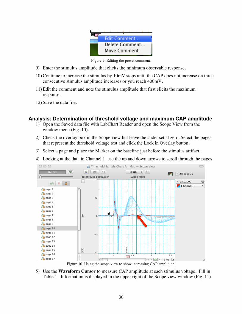
Figure 7. Proper set up of recording and stimulating leads.
Exercise 1: Determination of threshold voltage and maximal CAP amplitude In this part of the experiment, a series of stimuli will be given to the nerve, each increasing in amplitude. From these recordings the threshold voltage for the nerve will be calculated, as well as the voltage required for maximum CAP amplitude.
1) From the LabChart Welcome Center, select the Threshold settings file. 2) You will now use LabChart to stimulate the nerve and record 20 blocks of data. 3) Click start, No response should be seen. 4) In the Stimulator Panel, (Fig. 8) set the amplitude to 10mV; do not adjust any other
parameters.
Figure 8. Stimulator Panel
5) Click Start. 6) Increase the stimulus amplitude by 10mV, Click start. 7) Repeat this until a response is seen or you reach 400mV. If you do not see a response,
consult your instructor. 8) When a response is seen, edit the comment by right clicking on the number box at the
bottom of the Comment and selecting Edit (Fig. 9).
30
Figure 9. Editing the preset comment.
9) Enter the stimulus amplitude that elicits the minimum observable response. 10) Continue to increase the stimulus by 10mV steps until the CAP does not increase on three
consecutive stimulus amplitude increases or you reach 400mV. 11) Edit the comment and note the stimulus amplitude that first elicits the maximum
response. 12) Save the data file.
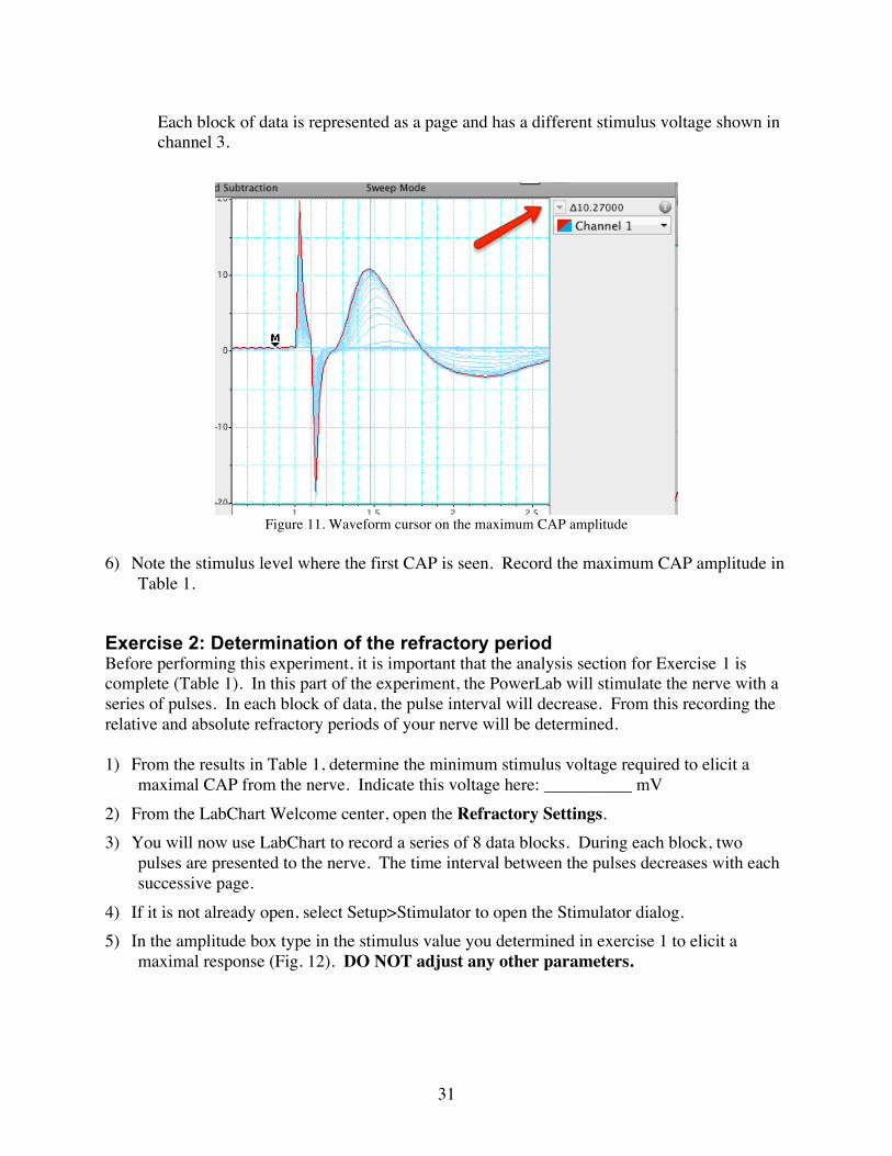
Analysis: Determination of threshold voltage and maximum CAP amplitude 1) Open the Saved data file with LabChart Reader and open the Scope View from the
window menu (Fig. 10). 2) Check the overlay box in the Scope view but leave the slider set at zero. Select the pages
that represent the threshold voltage test and click the Lock in Overlay button. 3) Select a page and place the Marker on the baseline just before the stimulus artifact. 4) Looking at the data in Channel 1, use the up and down arrows to scroll through the pages.
Figure 10. Using the scope view to show increasing CAP amplitude.
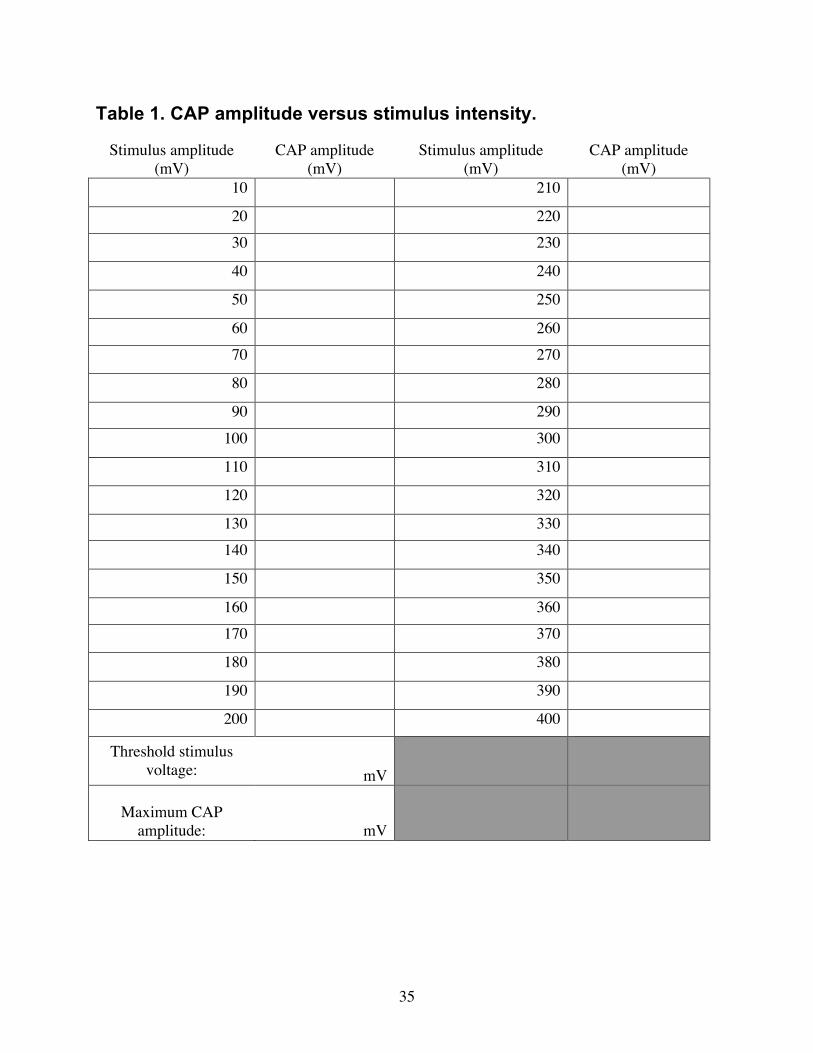
5) Use the Waveform Cursor to measure CAP amplitude at each stimulus voltage, Fill in Table 1. Information is displayed in the upper right of the Scope view window (Fig. 11).
31
Each block of data is represented as a page and has a different stimulus voltage shown in channel 3.
Figure 11. Waveform cursor on the maximum CAP amplitude
6) Note the stimulus level where the first CAP is seen. Record the maximum CAP amplitude in
Table 1.
Exercise 2: Determination of the refractory period Before performing this experiment, it is important that the analysis section for Exercise 1 is complete (Table 1). In this part of the experiment, the PowerLab will stimulate the nerve with a series of pulses. In each block of data, the pulse interval will decrease. From this recording the relative and absolute refractory periods of your nerve will be determined. 1) From the results in Table 1, determine the minimum stimulus voltage required to elicit a
maximal CAP from the nerve. Indicate this voltage here: __________ mV 2) From the LabChart Welcome center, open the Refractory Settings. 3) You will now use LabChart to record a series of 8 data blocks. During each block, two
pulses are presented to the nerve. The time interval between the pulses decreases with each successive page.
4) If it is not already open, select Setup>Stimulator to open the Stimulator dialog. 5) In the amplitude box type in the stimulus value you determined in exercise 1 to elicit a
maximal response (Fig. 12). DO NOT adjust any other parameters.

32
Figure 12. The stimulator dialog, you will enter the amplitude value from exercise 1, and then adjust the interval
between the 2 pulses. DO NOT adjust any other parameters.
6) Click Start, LabChart will stimulate the nerve 2 times 4 milliseconds apart. 7) Change the interval between pulses to 3.5ms, click Start. 8) Repeat for each specified interval Table 2 in the Data Notebook. 9) Save the data file.
Exercise 3: Determination of nerve conduction velocity In this part of the experiment, the velocity of the CAP as it travels down the nerve will be calculated.
1) Using a ruler, measure the distance in centimeters between the black negative leads of each of the two recording electrodes. Record this value in Table 3.
2) Follow the directions from the Analysis section below. Using data from a maximum CAP recorded during the threshold experiment, fill in Table 3.
3) After all recordings have been made, return the nerve to its dish of cold frog Ringer’s solution and return the nerve to your instructor.
Analysis Determination of refractory period
1. Select the CAPs recorded in channel 1 in each block of data recorded in Exercise 2. 2. Open the Zoom window and examine the data trace using the Waveform Cursor. (Fig.
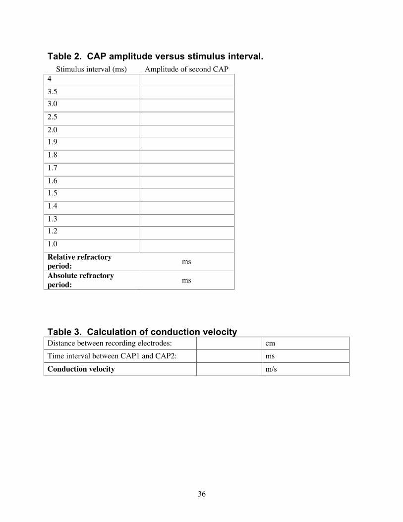
13). 3. Record the amplitude for the second CAP in Table 2 of the Data Notebook.
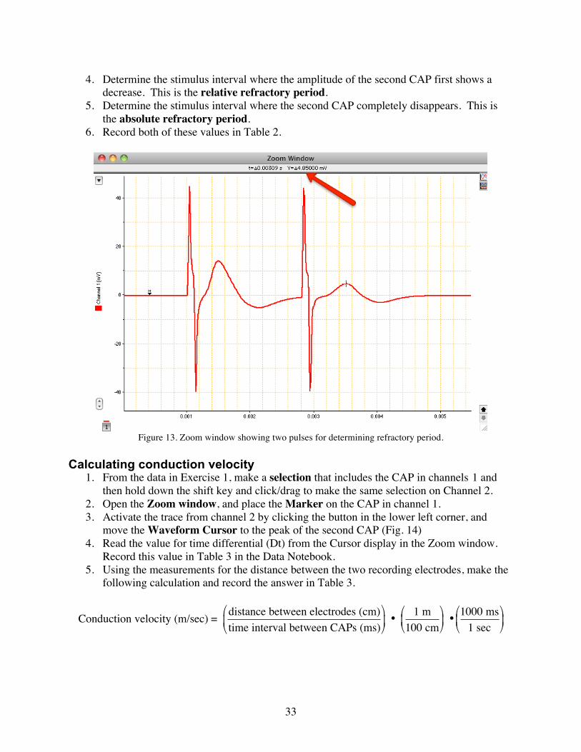
33
4. Determine the stimulus interval where the amplitude of the second CAP first shows a decrease. This is the relative refractory period.
5. Determine the stimulus interval where the second CAP completely disappears. This is the absolute refractory period.
6. Record both of these values in Table 2.
Figure 13. Zoom window showing two pulses for determining refractory period.
Calculating conduction velocity
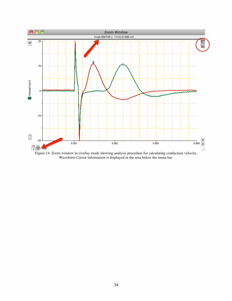
1. From the data in Exercise 1, make a selection that includes the CAP in channels 1 and then hold down the shift key and click/drag to make the same selection on Channel 2.
2. Open the Zoom window, and place the Marker on the CAP in channel 1. 3. Activate the trace from channel 2 by clicking the button in the lower left corner, and
move the Waveform Cursor to the peak of the second CAP (Fig. 14) 4. Read the value for time differential (Dt) from the Cursor display in the Zoom window.
Record this value in Table 3 in the Data Notebook. 5. Using the measurements for the distance between the two recording electrodes, make the
following calculation and record the answer in Table 3.
!
Conduction velocity (m/sec) = distance between electrodes (cm)time interval between CAPs (ms)"
# $
%
& ' • 1 m
100 cm"
# $
%
& ' •
1000 ms1 sec
"
# $
%
& '
34
Figure 14. Zoom window in overlay mode showing analysis procedure for calculating conduction velocity.
Waveform Cursor information is displayed in the area below the menu bar.
35
Table 1. CAP amplitude versus stimulus intensity.
Stimulus amplitude (mV)
CAP amplitude (mV)
Stimulus amplitude (mV)
CAP amplitude (mV)
10 210
20 220 30 230
40 240
50 250
60 260 70 270
80 280
90 290 100 300
110 310
120 320
130 330 140 340
150 350
160 360 170 370
180 380
190 390
200 400
Threshold stimulus voltage: mV
Maximum CAP amplitude: mV
36
Table 2. CAP amplitude versus stimulus interval. Stimulus interval (ms) Amplitude of second CAP
4 3.5 3.0 2.5 2.0 1.9 1.8 1.7 1.6 1.5 1.4 1.3 1.2 1.0 Relative refractory period: ms
Absolute refractory period: ms
Table 3. Calculation of conduction velocity Distance between recording electrodes: cm Time interval between CAP1 and CAP2: ms Conduction velocity m/s
37
Study Questions Answer the following questions in complete sentences. 1. How does a CAP differ from a single action potential?
2. What is the cause the A. relative, and B. the absolute refractory period?
3. Action potentials are said to be “all or none” responses. Why does the frog sciatic nerve give a graded response?
4. Briefly describe the cellular events that occur during the refractory period.
38
Muscle Stimulation & Fatigue
In this experiment, you will explore muscle function through stimulation and fatigue. You will electrically stimulate the nerves in the forearm to demonstrate recruitment, summation, and tetanus. (Written by the staff of ADInstruments).
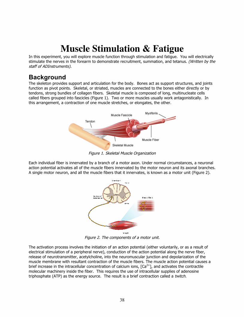
Background The skeleton provides support and articulation for the body. Bones act as support structures, and joints function as pivot points. Skeletal, or striated, muscles are connected to the bones either directly or by tendons, strong bundles of collagen fibers. Skeletal muscle is composed of long, multinucleate cells called fibers grouped into fascicles (Figure 1). Two or more muscles usually work antagonistically. In this arrangement, a contraction of one muscle stretches, or elongates, the other.
Figure 1. Skeletal Muscle Organization
Each individual fiber is innervated by a branch of a motor axon. Under normal circumstances, a neuronal action potential activates all of the muscle fibers innervated by the motor neuron and its axonal branches. A single motor neuron, and all the muscle fibers that it innervates, is known as a motor unit (Figure 2).
Figure 2. The components of a motor unit.
The activation process involves the initiation of an action potential (either voluntarily, or as a result of electrical stimulation of a peripheral nerve), conduction of the action potential along the nerve fiber, release of neurotransmitter, acetylcholine, into the neuromuscular junction and depolarization of the muscle membrane with resultant contraction of the muscle fibers. The muscle action potential causes a brief increase in the intracellular concentration of calcium ions, [Ca2+], and activates the contractile molecular machinery inside the fiber. This requires the use of intracellular supplies of adenosine triphosphate (ATP) as the energy source. The result is a brief contraction called a twitch.
39
A whole muscle is controlled by the firing of up to hundreds of motor axons. These motor nerves control movement in a variety of ways. One way in which the nervous system controls a muscle is by adjusting the number of motor axons firing, thus controlling the number of twitching muscle fibers. This process is called recruitment. A second way the nervous system controls a muscle contraction is to vary the frequency of action potentials in the motor axons. At stimulation intervals greater than 200 ms, intracellular [Ca2+] is restored to baseline levels between action potentials, and the contraction consists of separate twitches. At stimulation intervals between 200 and 75 ms, [Ca2+] in the muscle is still above baseline levels when the next action potential arrives. The muscle fiber, therefore, has not completely relaxed and the next contraction is stronger than normal. This additive effect is called summation. At even higher stimulation frequencies, the muscle has no time to relax between successive stimuli. The result is a smooth contraction many times stronger than a single twitch, called a tetanic contraction. The muscle is now in a state of tetanus.
Required Equipment • LabChart software • PowerLab Data Acquisition Unit • Finger Pulse Transducer • Hand Dynamometer
• Stimulating Bar Electrode • Electrode Cream or Paste • Medical tape
Procedure This experiment involves application of electrical shocks to muscle through electrodes
placed on the skin. Students who have cardiac pacemakers or who suffer from neurological or cardiac disorders should not volunteer for this exercise. If the volunteer feels major discomfort during the exercise, discontinue the exercise and consult your instructor.
Equipment Setup 1. Make sure the PowerLab is turned off and the USB cable is connected to the computer.
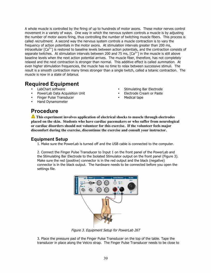
2. Connect the Finger Pulse Transducer to Input 1 on the front panel of the PowerLab and the Stimulating Bar Electrode to the Isolated Stimulator output on the front panel (Figure 3). Make sure the red (positive) connector is in the red output and the black (negative) connector is in the black output. The hardware needs to be connected before you open the settings file.
Figure 3. Equipment Setup for PowerLab 26T
3. Place the pressure pad of the Finger Pulse Transducer on the top of the table. Tape the transducer in place along the Velcro strap. The Finger Pulse Transducer needs to be close to
40
the edge of the table (Figure 3). If the table is too thick for the volunteer to grasp, a different flat surface will have to be used.
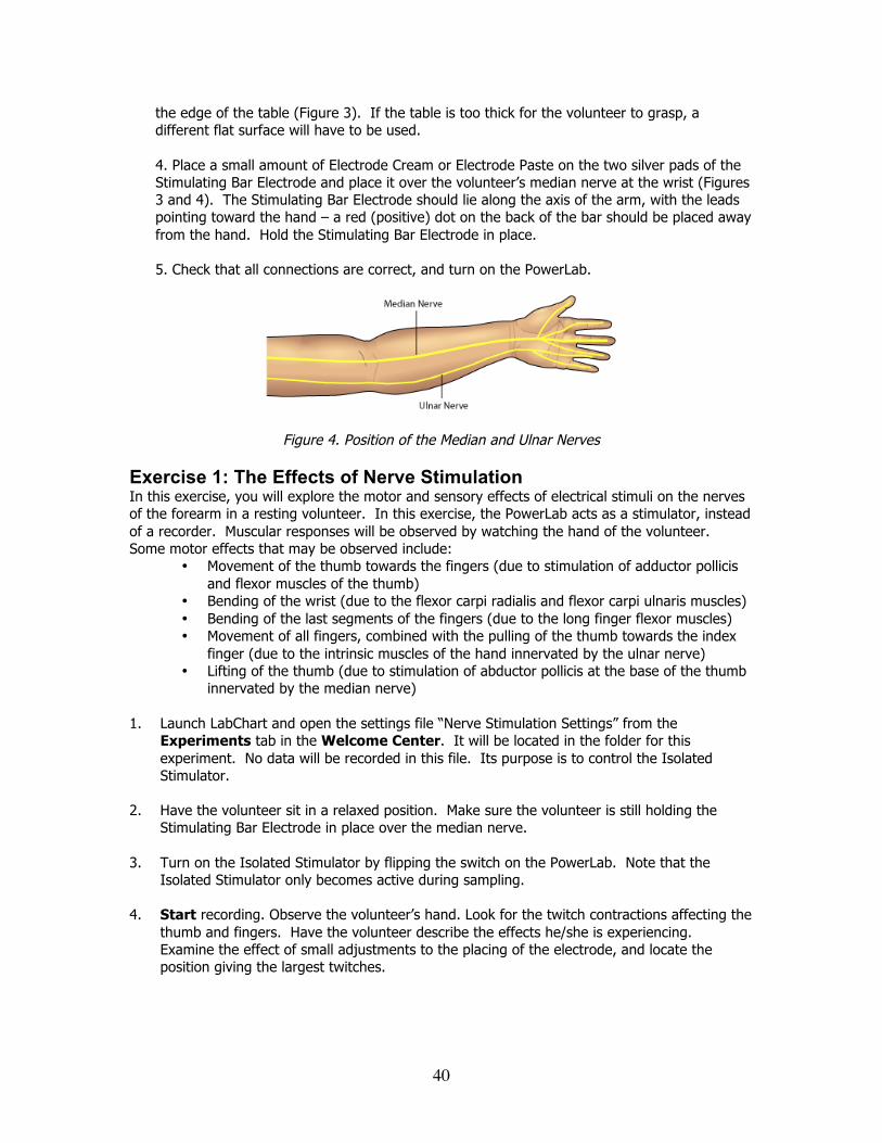
4. Place a small amount of Electrode Cream or Electrode Paste on the two silver pads of the Stimulating Bar Electrode and place it over the volunteer’s median nerve at the wrist (Figures 3 and 4). The Stimulating Bar Electrode should lie along the axis of the arm, with the leads pointing toward the hand – a red (positive) dot on the back of the bar should be placed away from the hand. Hold the Stimulating Bar Electrode in place.
5. Check that all connections are correct, and turn on the PowerLab.
Figure 4. Position of the Median and Ulnar Nerves
Exercise 1: The Effects of Nerve Stimulation In this exercise, you will explore the motor and sensory effects of electrical stimuli on the nerves of the forearm in a resting volunteer. In this exercise, the PowerLab acts as a stimulator, instead of a recorder. Muscular responses will be observed by watching the hand of the volunteer. Some motor effects that may be observed include:
• Movement of the thumb towards the fingers (due to stimulation of adductor pollicis and flexor muscles of the thumb)
• Bending of the wrist (due to the flexor carpi radialis and flexor carpi ulnaris muscles) • Bending of the last segments of the fingers (due to the long finger flexor muscles) • Movement of all fingers, combined with the pulling of the thumb towards the index
finger (due to the intrinsic muscles of the hand innervated by the ulnar nerve) • Lifting of the thumb (due to stimulation of abductor pollicis at the base of the thumb
innervated by the median nerve) 1. Launch LabChart and open the settings file “Nerve Stimulation Settings” from the
Experiments tab in the Welcome Center. It will be located in the folder for this experiment. No data will be recorded in this file. Its purpose is to control the Isolated Stimulator.
2. Have the volunteer sit in a relaxed position. Make sure the volunteer is still holding the Stimulating Bar Electrode in place over the median nerve.
3. Turn on the Isolated Stimulator by flipping the switch on the PowerLab. Note that the Isolated Stimulator only becomes active during sampling.
4. Start recording. Observe the volunteer’s hand. Look for the twitch contractions affecting the thumb and fingers. Have the volunteer describe the effects he/she is experiencing. Examine the effect of small adjustments to the placing of the electrode, and locate the position giving the largest twitches.
41
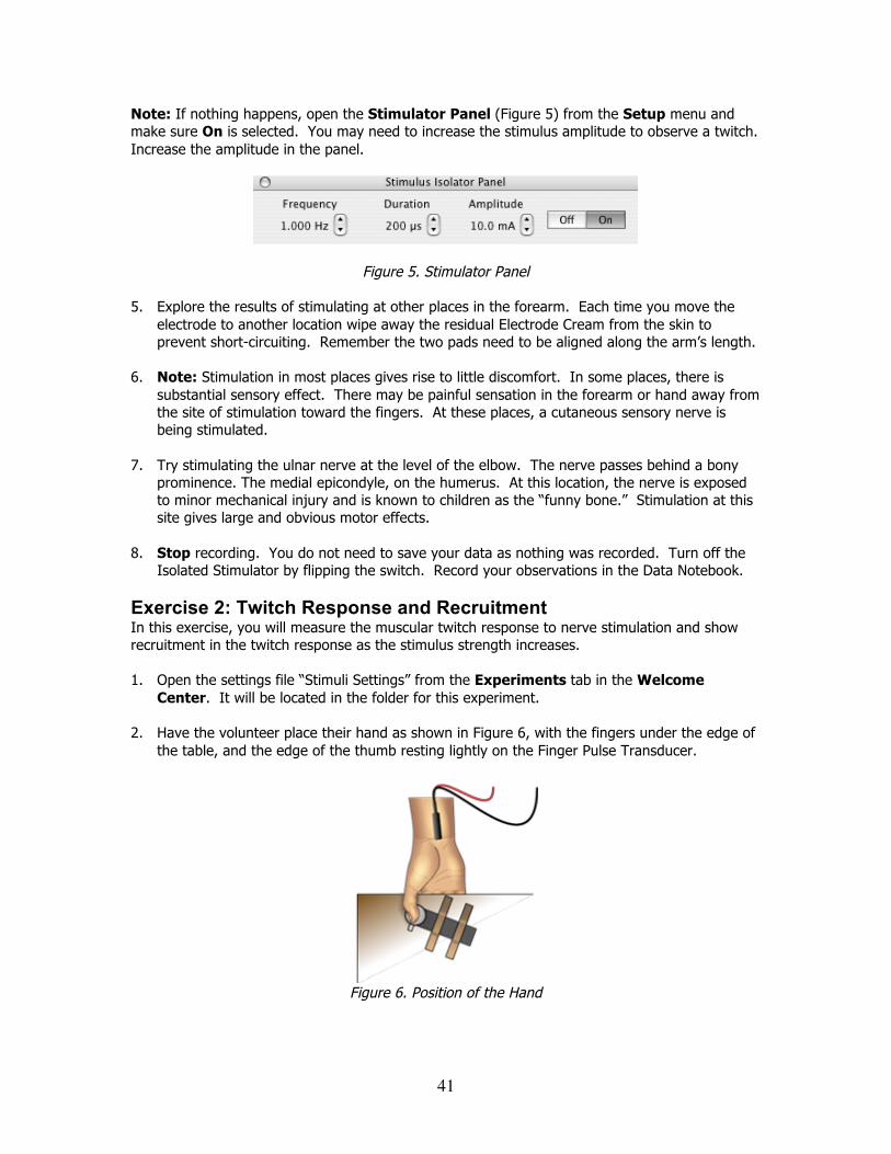
Note: If nothing happens, open the Stimulator Panel (Figure 5) from the Setup menu and make sure On is selected. You may need to increase the stimulus amplitude to observe a twitch. Increase the amplitude in the panel.
Figure 5. Stimulator Panel
5. Explore the results of stimulating at other places in the forearm. Each time you move the electrode to another location wipe away the residual Electrode Cream from the skin to prevent short-circuiting. Remember the two pads need to be aligned along the arm’s length.
6. Note: Stimulation in most places gives rise to little discomfort. In some places, there is substantial sensory effect. There may be painful sensation in the forearm or hand away from the site of stimulation toward the fingers. At these places, a cutaneous sensory nerve is being stimulated.
7. Try stimulating the ulnar nerve at the level of the elbow. The nerve passes behind a bony prominence. The medial epicondyle, on the humerus. At this location, the nerve is exposed to minor mechanical injury and is known to children as the “funny bone.” Stimulation at this site gives large and obvious motor effects.
8. Stop recording. You do not need to save your data as nothing was recorded. Turn off the Isolated Stimulator by flipping the switch. Record your observations in the Data Notebook.
Exercise 2: Twitch Response and Recruitment In this exercise, you will measure the muscular twitch response to nerve stimulation and show recruitment in the twitch response as the stimulus strength increases. 1. Open the settings file “Stimuli Settings” from the Experiments tab in the Welcome
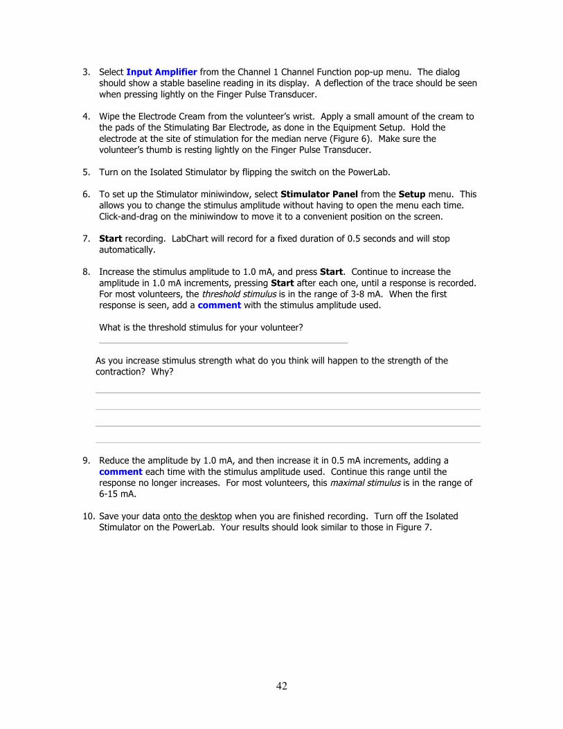
Center. It will be located in the folder for this experiment. 2. Have the volunteer place their hand as shown in Figure 6, with the fingers under the edge of
the table, and the edge of the thumb resting lightly on the Finger Pulse Transducer.
Figure 6. Position of the Hand
42
3. Select Input Amplifier from the Channel 1 Channel Function pop-up menu. The dialog should show a stable baseline reading in its display. A deflection of the trace should be seen when pressing lightly on the Finger Pulse Transducer.
4. Wipe the Electrode Cream from the volunteer’s wrist. Apply a small amount of the cream to
the pads of the Stimulating Bar Electrode, as done in the Equipment Setup. Hold the electrode at the site of stimulation for the median nerve (Figure 6). Make sure the volunteer’s thumb is resting lightly on the Finger Pulse Transducer.
5. Turn on the Isolated Stimulator by flipping the switch on the PowerLab.
6. To set up the Stimulator miniwindow, select Stimulator Panel from the Setup menu. This allows you to change the stimulus amplitude without having to open the menu each time. Click-and-drag on the miniwindow to move it to a convenient position on the screen.
7. Start recording. LabChart will record for a fixed duration of 0.5 seconds and will stop automatically.
8. Increase the stimulus amplitude to 1.0 mA, and press Start. Continue to increase the amplitude in 1.0 mA increments, pressing Start after each one, until a response is recorded. For most volunteers, the threshold stimulus is in the range of 3-8 mA. When the first response is seen, add a comment with the stimulus amplitude used.
What is the threshold stimulus for your volunteer?
As you increase stimulus strength what do you think will happen to the strength of the contraction? Why?
9. Reduce the amplitude by 1.0 mA, and then increase it in 0.5 mA increments, adding a comment each time with the stimulus amplitude used. Continue this range until the response no longer increases. For most volunteers, this maximal stimulus is in the range of 6-15 mA.
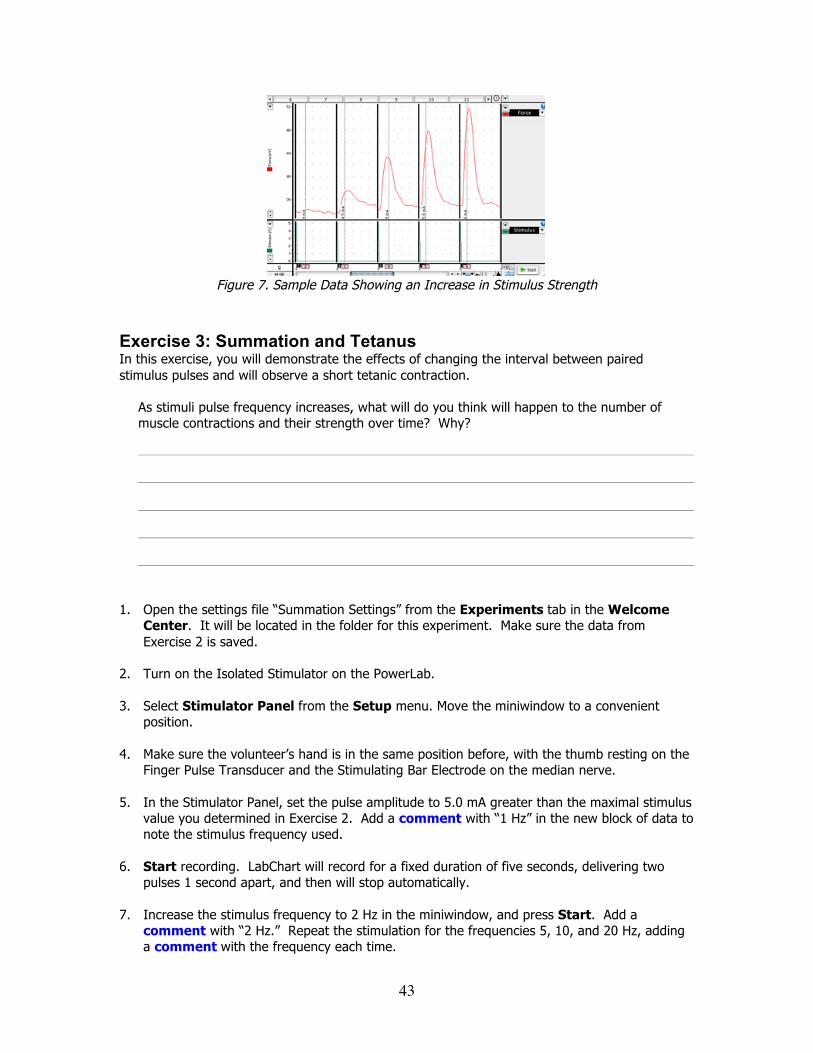
10. Save your data onto the desktop when you are finished recording. Turn off the Isolated Stimulator on the PowerLab. Your results should look similar to those in Figure 7.
43
Figure 7. Sample Data Showing an Increase in Stimulus Strength
Exercise 3: Summation and Tetanus In this exercise, you will demonstrate the effects of changing the interval between paired stimulus pulses and will observe a short tetanic contraction.
As stimuli pulse frequency increases, what will do you think will happen to the number of muscle contractions and their strength over time? Why?
1. Open the settings file “Summation Settings” from the Experiments tab in the Welcome
Center. It will be located in the folder for this experiment. Make sure the data from Exercise 2 is saved.
2. Turn on the Isolated Stimulator on the PowerLab.
3. Select Stimulator Panel from the Setup menu. Move the miniwindow to a convenient
position.
4. Make sure the volunteer’s hand is in the same position before, with the thumb resting on the Finger Pulse Transducer and the Stimulating Bar Electrode on the median nerve.
5. In the Stimulator Panel, set the pulse amplitude to 5.0 mA greater than the maximal stimulus
value you determined in Exercise 2. Add a comment with “1 Hz” in the new block of data to note the stimulus frequency used.
6. Start recording. LabChart will record for a fixed duration of five seconds, delivering two
pulses 1 second apart, and then will stop automatically. 7. Increase the stimulus frequency to 2 Hz in the miniwindow, and press Start. Add a
comment with “2 Hz.” Repeat the stimulation for the frequencies 5, 10, and 20 Hz, adding a comment with the frequency each time.
44
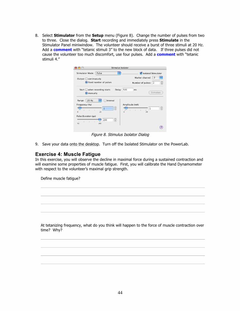
8. Select Stimulator from the Setup menu (Figure 8). Change the number of pulses from two
to three. Close the dialog. Start recording and immediately press Stimulate in the Stimulator Panel miniwindow. The volunteer should receive a burst of three stimuli at 20 Hz. Add a comment with “tetanic stimuli 3” to the new block of data. If three pulses did not cause the volunteer too much discomfort, use four pulses. Add a comment with “tetanic stimuli 4.”
Figure 8. Stimulus Isolator Dialog
9. Save your data onto the desktop. Turn off the Isolated Stimulator on the PowerLab. Exercise 4: Muscle Fatigue In this exercise, you will observe the decline in maximal force during a sustained contraction and will examine some properties of muscle fatigue. First, you will calibrate the Hand Dynamometer with respect to the volunteer’s maximal grip strength.
Define muscle fatigue?
At tetanizing frequency, what do you think will happen to the force of muscle contraction over time? Why?
45
If you let the muscle rest of a short period of time after a tetanizing frequency stimulus, what do you think will happen to the force of muscle contraction? Why?
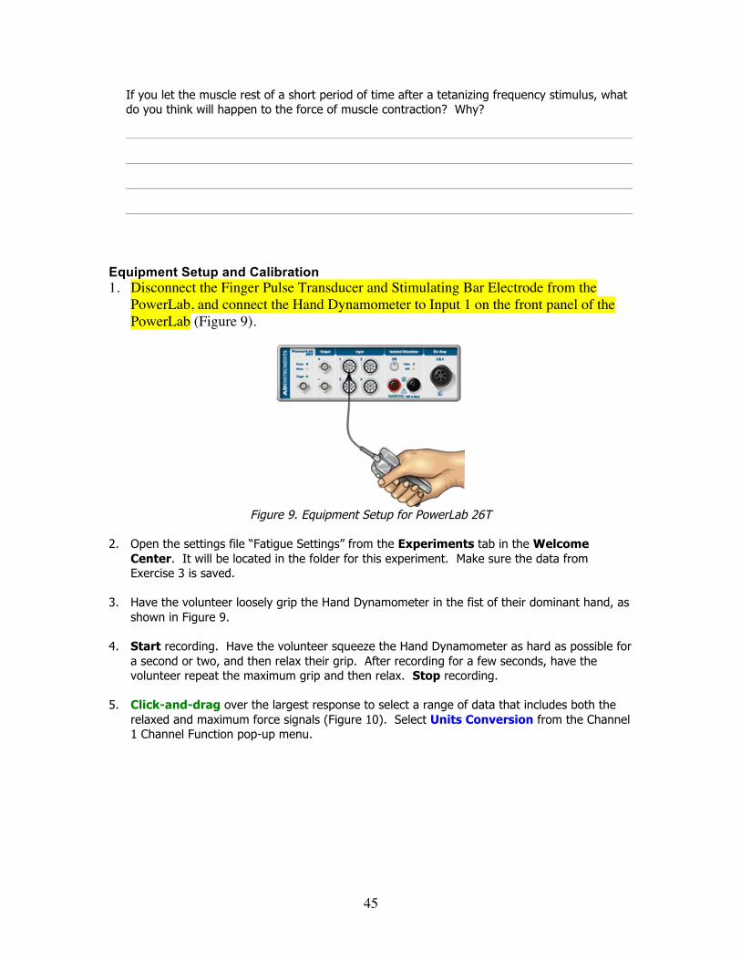
Equipment Setup and Calibration 1. Disconnect the Finger Pulse Transducer and Stimulating Bar Electrode from the
PowerLab, and connect the Hand Dynamometer to Input 1 on the front panel of the PowerLab (Figure 9).
Figure 9. Equipment Setup for PowerLab 26T
2. Open the settings file “Fatigue Settings” from the Experiments tab in the Welcome
Center. It will be located in the folder for this experiment. Make sure the data from Exercise 3 is saved.
3. Have the volunteer loosely grip the Hand Dynamometer in the fist of their dominant hand, as shown in Figure 9.
4. Start recording. Have the volunteer squeeze the Hand Dynamometer as hard as possible for
a second or two, and then relax their grip. After recording for a few seconds, have the volunteer repeat the maximum grip and then relax. Stop recording.
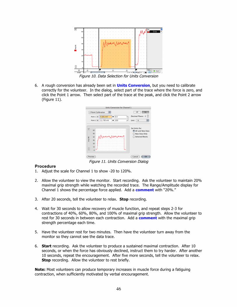
5. Click-and-drag over the largest response to select a range of data that includes both the
relaxed and maximum force signals (Figure 10). Select Units Conversion from the Channel 1 Channel Function pop-up menu.
46
Figure 10. Data Selection for Units Conversion
6. A rough conversion has already been set in Units Conversion, but you need to calibrate
correctly for the volunteer. In the dialog, select part of the trace where the force is zero, and click the Point 1 arrow. Then select part of the trace at the peak, and click the Point 2 arrow (Figure 11).
Figure 11. Units Conversion Dialog
Procedure 1. Adjust the scale for Channel 1 to show -20 to 120%. 2. Allow the volunteer to view the monitor. Start recording. Ask the volunteer to maintain 20%
maximal grip strength while watching the recorded trace. The Range/Amplitude display for Channel 1 shows the percentage force applied. Add a comment with “20%.”
3. After 20 seconds, tell the volunteer to relax. Stop recording. 4. Wait for 30 seconds to allow recovery of muscle function, and repeat steps 2-3 for
contractions of 40%, 60%, 80%, and 100% of maximal grip strength. Allow the volunteer to rest for 30 seconds in between each contraction. Add a comment with the maximal grip strength percentage each time.
5. Have the volunteer rest for two minutes. Then have the volunteer turn away from the
monitor so they cannot see the data trace. 6. Start recording. Ask the volunteer to produce a sustained maximal contraction. After 10
seconds, or when the force has obviously declined, instruct them to try harder. After another 10 seconds, repeat the encouragement. After five more seconds, tell the volunteer to relax. Stop recording. Allow the volunteer to rest briefly.
Note: Most volunteers can produce temporary increases in muscle force during a fatiguing contraction, when sufficiently motivated by verbal encouragement.
47
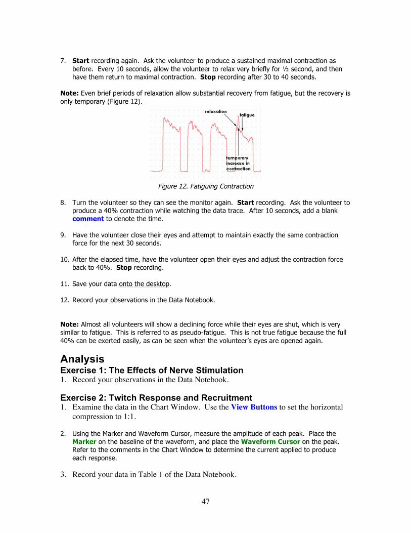
7. Start recording again. Ask the volunteer to produce a sustained maximal contraction as
before. Every 10 seconds, allow the volunteer to relax very briefly for ½ second, and then have them return to maximal contraction. Stop recording after 30 to 40 seconds.
Note: Even brief periods of relaxation allow substantial recovery from fatigue, but the recovery is only temporary (Figure 12).
Figure 12. Fatiguing Contraction
8. Turn the volunteer so they can see the monitor again. Start recording. Ask the volunteer to
produce a 40% contraction while watching the data trace. After 10 seconds, add a blank comment to denote the time.
9. Have the volunteer close their eyes and attempt to maintain exactly the same contraction
force for the next 30 seconds. 10. After the elapsed time, have the volunteer open their eyes and adjust the contraction force
back to 40%. Stop recording. 11. Save your data onto the desktop. 12. Record your observations in the Data Notebook.
Note: Almost all volunteers will show a declining force while their eyes are shut, which is very similar to fatigue. This is referred to as pseudo-fatigue. This is not true fatigue because the full 40% can be exerted easily, as can be seen when the volunteer’s eyes are opened again.
Analysis Exercise 1: The Effects of Nerve Stimulation 1. Record your observations in the Data Notebook.
Exercise 2: Twitch Response and Recruitment 1. Examine the data in the Chart Window. Use the View Buttons to set the horizontal
compression to 1:1.
2. Using the Marker and Waveform Cursor, measure the amplitude of each peak. Place the Marker on the baseline of the waveform, and place the Waveform Cursor on the peak. Refer to the comments in the Chart Window to determine the current applied to produce each response.
3. Record your data in Table 1 of the Data Notebook.

48
Exercise 3: Summation and Tetanus 1. Examine the data in the Chart View, and Autoscale, if necessary. 2. Calculate the stimulus interval for each stimulation frequency using the following equation:
!
interval (sec) = 1f ,
where f is the stimulus frequency (Hz) 3. Using the Marker and Waveform Cursor, measure the amplitude of the first two responses at
each stimulus interval. Place the Marker on the baseline of the waveform, and place the Waveform Cursor on the peak.
4. Record these values in Table 2 of the Data Notebook. 5. Examine the tetanic response. Calculate the stimulus interval, and record this value in Table
3 of the Data Notebook. 6. Click-and-drag the tetanic response, and examine it in Zoom Window. Determine the
maximum force amplitude using the Marker and Waveform Cursor, as before. 7. If the tetanus exercise was repeated with four pulses, repeat the analysis. 8. Record your data in Table 3 of the Data Notebook. If you did not use four pulses, leave this
part of the table blank. 9. Exercise 4: Muscle Fatigue 1. Examine the data in the Chart Window, and Autoscale, if necessary. 2. Record your observations in the Data Notebook.
49
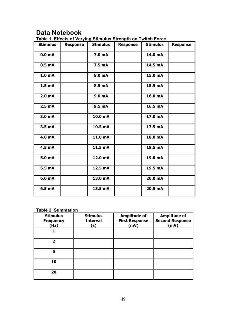
Data Notebook Table 1. Effects of Varying Stimulus Strength on Twitch Force
Stimulus
Response Stimulus Response Stimulus Response
0.0 mA
7.0 mA 14.0 mA
0.5 mA
7.5 mA 14.5 mA
1.0 mA
8.0 mA 15.0 mA
1.5 mA
8.5 mA 15.5 mA
2.0 mA
9.0 mA 16.0 mA
2.5 mA
9.5 mA 16.5 mA
3.0 mA
10.0 mA 17.0 mA
3.5 mA
10.5 mA 17.5 mA
4.0 mA
11.0 mA 18.0 mA
4.5 mA
11.5 mA 18.5 mA
5.0 mA
12.0 mA 19.0 mA
5.5 mA
12.5 mA 19.5 mA
6.0 mA
13.0 mA 20.0 mA
6.5 mA
13.5 mA 20.5 mA
Table 2. Summation
Stimulus Frequency
(Hz)
Stimulus Interval
(s)
Amplitude of First Response
(mV)
Amplitude of Second Response
(mV) 1
2
5
10
20
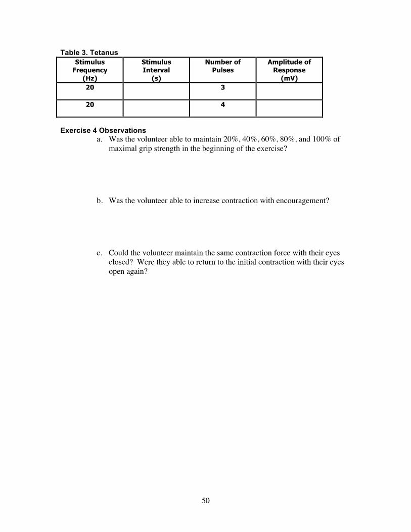
50
Table 3. Tetanus Stimulus
Frequency (Hz)
Stimulus Interval
(s)
Number of Pulses
Amplitude of Response
(mV) 20
3
20
4
Exercise 4 Observations
a. Was the volunteer able to maintain 20%, 40%, 60%, 80%, and 100% of maximal grip strength in the beginning of the exercise?
b. Was the volunteer able to increase contraction with encouragement?
c. Could the volunteer maintain the same contraction force with their eyes closed? Were they able to return to the initial contraction with their eyes open again?
51
Study Questions 1. What was the threshold stimulus of the volunteer? What was the maximal stimulus?
2. What can you conclude regarding the number of fibers contracting as the current was raised from threshold to that required for a maximal contraction?
3. Why does varying the stimulus strength affect the twitch force?
4. What are the two ways by which the nervous system can control the force generated by a muscle?

52
Hematology Introduction Blood provides a medium for homeostasis in the cells’ environment. Blood bathes cells within the body of vertebrates and transports O2 as well as nutrients to body cells whilst removing CO2 and waste products. This transport system also serves to link the various organ systems of an animal’s body together, integrating them through the action of hormones. Blood also performs other not so obvious functions such as providing buffers for acid-base balance, destroying foreign organisms by phagocytosis and antibody action, distributing and conserving body heat, and preventing its own loss through hemostatic (coagulation) mechanisms. Blood is composed of a liquid portion, the plasma, and formed elements (red, white cells and platelets). In humans, red blood cells (RBC’s) or erythrocytes make up about 45% of total blood volume, this figure is called the hematocrit. Leukocytes or white blood cells and platelets make up 1% of total blood volume, and the rest (about 55%) consists of plasma. Normal blood volume is approximately 8% of an animal’s weight and in a 70 Kg human, this equates to 5.6 L in volume. RBC’s contain the protein hemoglobin which enables them to carry O2 to body cells and CO2 away from the cells. In humans, the average amount of hemoglobin per 100 ml of red cells is 16 g. Blood contains 5 types of white cells (leukocytes), divided into granulocytes and agranulocytes. Granulocytes are named because they contain heavy pigmented granules in their cytoplasm, where as agranulocytes contain no visible granules. The figure below shows and lists the distinguishing features of each of the different types of WBC’s in humans.
Neutrophils: 65% of total WBC’s, three-lobed nucleus, small pink cytoplasmic granules, purple nucleus. Eosinophils: 2 – 4% of total WBC’s, bi-lobed nucleus, coarse red-orange cytoplasmic granules, blue-purple nucleus.

53
Basophils: 0.5% of total WBC’s, bi-lobed nucleus, large deep blue or reddish purple cytoplasmic granules, blue-black nucleus. Small lymphocyte: 25% of total WBC’s, very large, spherical nucleus surrounded by thin cytoplasm, light blue non-granular cytoplasm, deep blue or purple nucleus. Large lymphocyte: 3% of total WBC’s, large oval indented nucleus, light blue non-granular cytoplasm, dark purple nucleus. Monocyte: 3 – 7% of total WBC’s, large blue-gray non-granular cytoplasm, blue or purple nucleus. Objectives • To become familiar with classical methods of quantitative blood parameters such as examining blood hematocrit, hemoglobin concentration, RBC and WBC counts. • To be able to identify different types of WBC’s. Equipment available in lab Sheep’s blood Hematocrit tubes Hematocrit reader Hematocrit centrifuge Critoseal Tallquist paper Teco control reagent set (fridge) Cyanmethemoglobin standard (fridge) Teco Hemoglobin reagent (room temp) Spectrophotometer & cuvettes Hemocytometers Distilled water
Kimwipes 95% ethanol Counters Compound microscopes Glass slides and coverslips Pasteur pipettes 10 ml test tubes (24) Gilson P20, P1,000 5 ml pipettes RBC dilution (1:200 w/Gowers) WBC dilution (1:15 w/Turks)
Experimental procedure Hematocrit Each table should perform this procedure. Place a hematocrit tube in a tilted beaker of sheep’s blood. The blood will move into the tube by capillary action. Fill the tube 3/4 full. Use critoseal to seal one end of the tube. Your instructor will show you how to place the tube inside the hematocrit centrifuge. Remember to place the sealed end towards the outside of the centrifuge. Once centrifuged, use the hematocrit reader to read the percentage of RBC’s in the sample. Again, your instructor will show you how to read the sample. The hematocrit for my sample is: Hemoglobin determination 1. Tallquist method Every table should perform this test. This test uses a book of Tallquist blotting paper and a color comparison LabChart having different intensities of red. These intensities correspond to different concentrations of hemoglobin (Hb) found in blood. Obtain a drop of blood and place it on a piece of blotting paper. Before the blood dries, match its color with the closest color on the comparison Chart. The number by
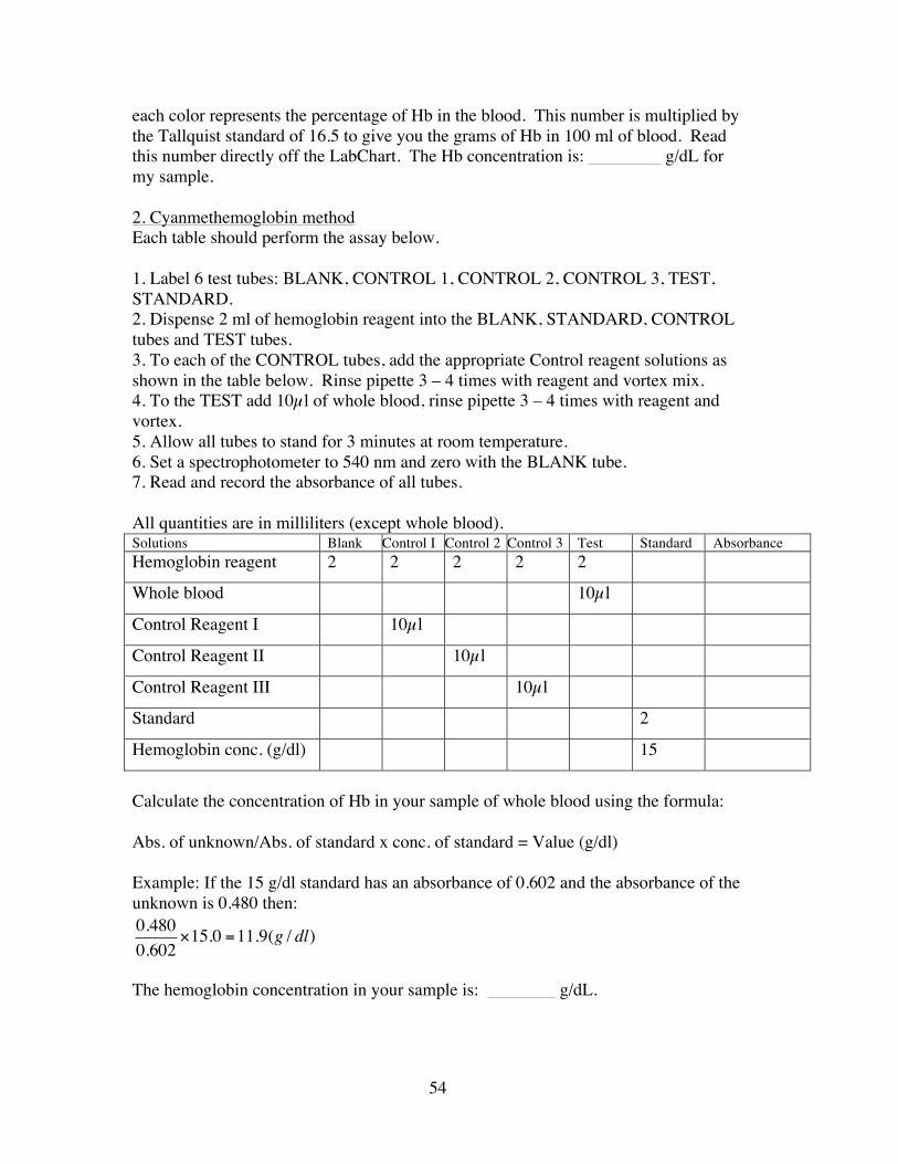
54
each color represents the percentage of Hb in the blood. This number is multiplied by the Tallquist standard of 16.5 to give you the grams of Hb in 100 ml of blood. Read this number directly off the LabChart. The Hb concentration is: g/dL for my sample. 2. Cyanmethemoglobin method Each table should perform the assay below. 1. Label 6 test tubes: BLANK, CONTROL 1, CONTROL 2, CONTROL 3, TEST, STANDARD. 2. Dispense 2 ml of hemoglobin reagent into the BLANK, STANDARD, CONTROL tubes and TEST tubes. 3. To each of the CONTROL tubes, add the appropriate Control reagent solutions as shown in the table below. Rinse pipette 3 – 4 times with reagent and vortex mix. 4. To the TEST add 10µl of whole blood, rinse pipette 3 – 4 times with reagent and vortex. 5. Allow all tubes to stand for 3 minutes at room temperature. 6. Set a spectrophotometer to 540 nm and zero with the BLANK tube. 7. Read and record the absorbance of all tubes. All quantities are in milliliters (except whole blood). Solutions Blank Control I Control 2 Control 3 Test Standard Absorbance Hemoglobin reagent 2 2 2 2 2
Whole blood 10µl
Control Reagent I 10µl
Control Reagent II 10µl
Control Reagent III 10µl
Standard 2
Hemoglobin conc. (g/dl) 15
Calculate the concentration of Hb in your sample of whole blood using the formula: Abs. of unknown/Abs. of standard x conc. of standard = Value (g/dl) Example: If the 15 g/dl standard has an absorbance of 0.602 and the absorbance of the unknown is 0.480 then: 0.4800.602
!15.0 =11.9(g / dl)
The hemoglobin concentration in your sample is: g/dL.
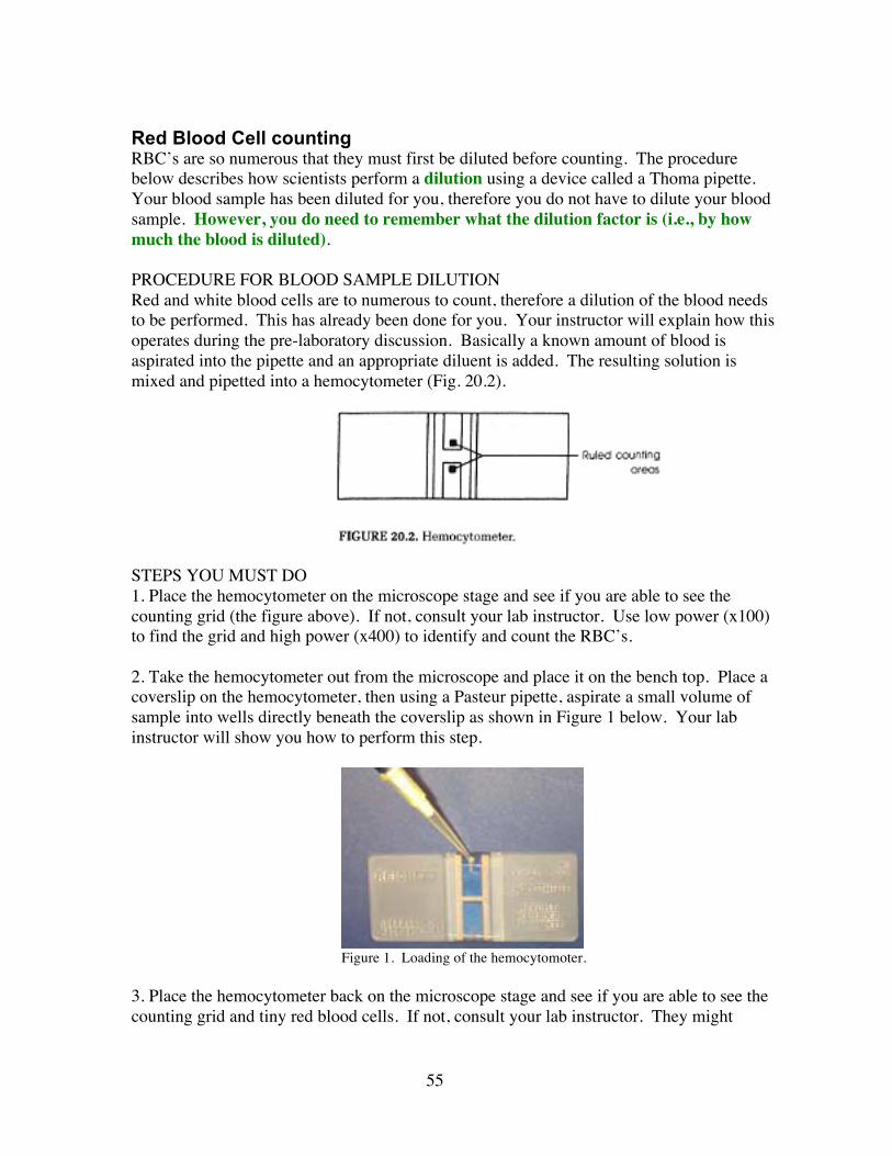
55
Red Blood Cell counting RBC’s are so numerous that they must first be diluted before counting. The procedure below describes how scientists perform a dilution using a device called a Thoma pipette. Your blood sample has been diluted for you, therefore you do not have to dilute your blood sample. However, you do need to remember what the dilution factor is (i.e., by how much the blood is diluted). PROCEDURE FOR BLOOD SAMPLE DILUTION Red and white blood cells are to numerous to count, therefore a dilution of the blood needs to be performed. This has already been done for you. Your instructor will explain how this operates during the pre-laboratory discussion. Basically a known amount of blood is aspirated into the pipette and an appropriate diluent is added. The resulting solution is mixed and pipetted into a hemocytometer (Fig. 20.2).
STEPS YOU MUST DO 1. Place the hemocytometer on the microscope stage and see if you are able to see the counting grid (the figure above). If not, consult your lab instructor. Use low power (x100) to find the grid and high power (x400) to identify and count the RBC’s. 2. Take the hemocytometer out from the microscope and place it on the bench top. Place a coverslip on the hemocytometer, then using a Pasteur pipette, aspirate a small volume of sample into wells directly beneath the coverslip as shown in Figure 1 below. Your lab instructor will show you how to perform this step.
Figure 1. Loading of the hemocytomoter.
3. Place the hemocytometer back on the microscope stage and see if you are able to see the counting grid and tiny red blood cells. If not, consult your lab instructor. They might
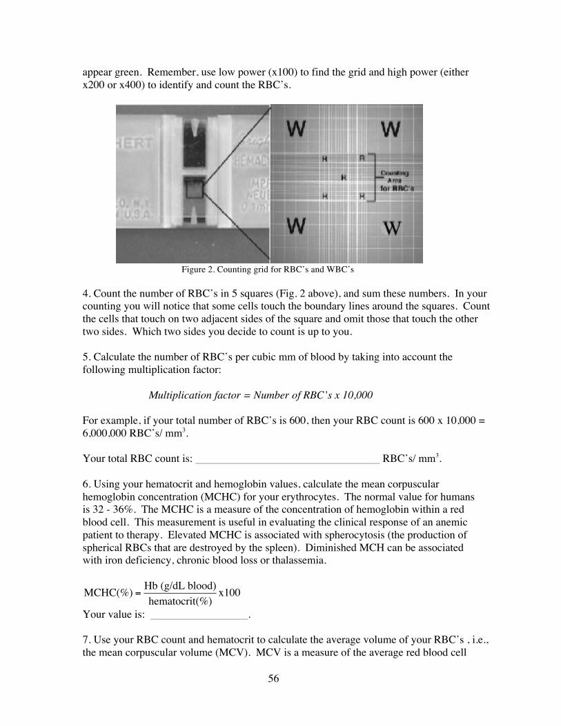
56
appear green. Remember, use low power (x100) to find the grid and high power (either x200 or x400) to identify and count the RBC’s.
Figure 2. Counting grid for RBC’s and WBC’s
4. Count the number of RBC’s in 5 squares (Fig. 2 above), and sum these numbers. In your counting you will notice that some cells touch the boundary lines around the squares. Count the cells that touch on two adjacent sides of the square and omit those that touch the other two sides. Which two sides you decide to count is up to you. 5. Calculate the number of RBC’s per cubic mm of blood by taking into account the following multiplication factor:
Multiplication factor = Number of RBC’s x 10,000 For example, if your total number of RBC’s is 600, then your RBC count is 600 x 10,000 = 6,000,000 RBC’s/ mm3. Your total RBC count is: RBC’s/ mm3. 6. Using your hematocrit and hemoglobin values, calculate the mean corpuscular hemoglobin concentration (MCHC) for your erythrocytes. The normal value for humans is 32 - 36%. The MCHC is a measure of the concentration of hemoglobin within a red blood cell. This measurement is useful in evaluating the clinical response of an anemic patient to therapy. Elevated MCHC is associated with spherocytosis (the production of spherical RBCs that are destroyed by the spleen). Diminished MCH can be associated with iron deficiency, chronic blood loss or thalassemia.
!
MCHC(%) =Hb (g/dL blood)hematocrit(%)
x100 Your value is: . 7. Use your RBC count and hematocrit to calculate the average volume of your RBC’s , i.e., the mean corpuscular volume (MCV). MCV is a measure of the average red blood cell

57
volume (i.e. size). The average value for humans is 87µm3 with a range from 80 – 96 µm3. The MCV is elevated if RBCs are larger than normal (macrocytic), for example in anemia caused by vitamin B12 deficiency. When the MCV is decreased, RBCs are smaller than normal (microcytic) as is seen in iron deficiency anemia or thalassemia.
!
MCV( 3µm ) =Hematocrit (%RBC) x 10
3RBC count (millions/mm )
Your value is: . The above measures are useful because anemia may be caused by several factors, such as RBC frailty, maturation deficiency and hemorrhage. The above measures allow one to classify the types of anemia more precisely. White blood cell count This technique is similar to that for determining RBC number except you must count and total the number of white cells in the 4 squares shown in Fig. 20.3 (above). To calculate the number of WBC’s per cubic millimeter, sum the total number of WBC’s in all 4 squares and multiply by 50.
Multiplication factor = Number of WBC’s x 50 Your total WBC count was: WBC’s/ mm3.
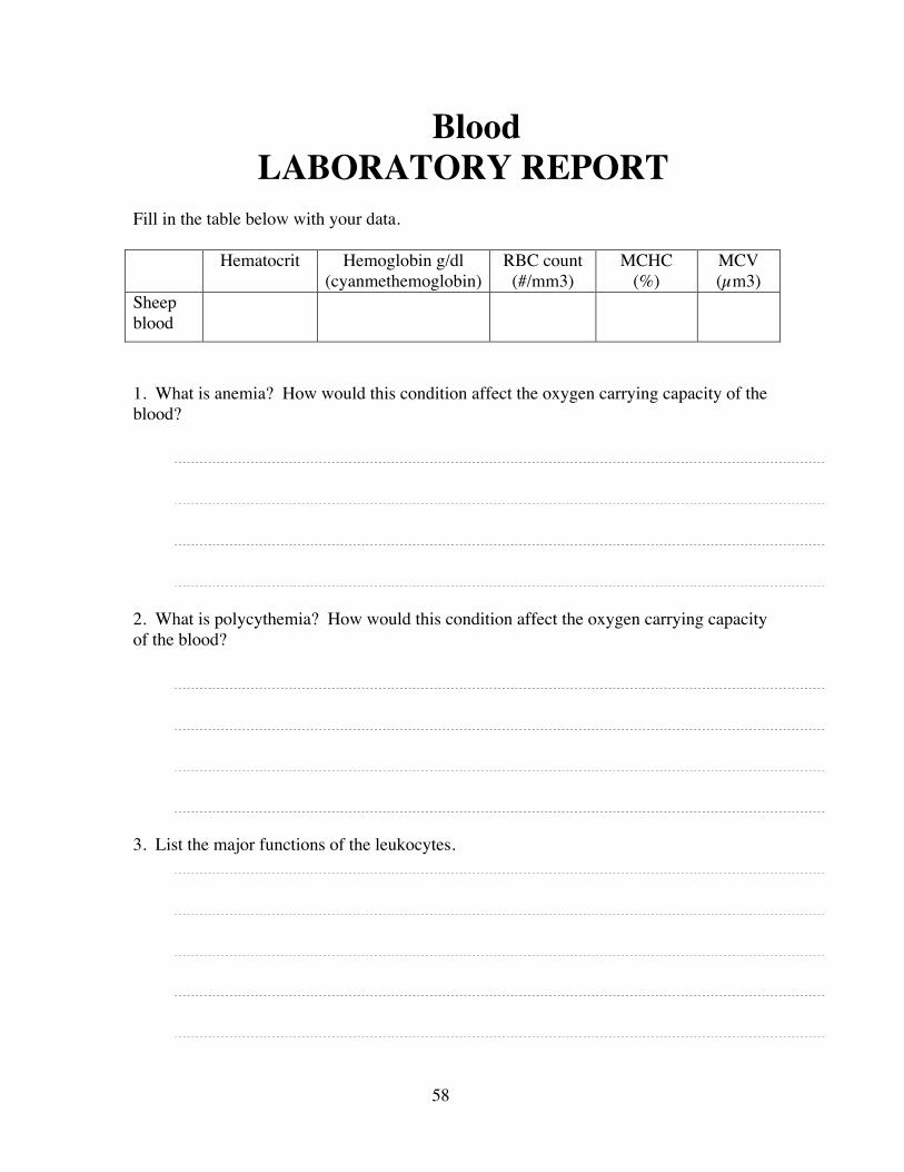
58
Blood LABORATORY REPORT
Fill in the table below with your data. Hematocrit Hemoglobin g/dl
(cyanmethemoglobin) RBC count (#/mm3)
MCHC (%)
MCV (µm3)
Sheep blood
1. What is anemia? How would this condition affect the oxygen carrying capacity of the blood?
2. What is polycythemia? How would this condition affect the oxygen carrying capacity of the blood?
3. List the major functions of the leukocytes.
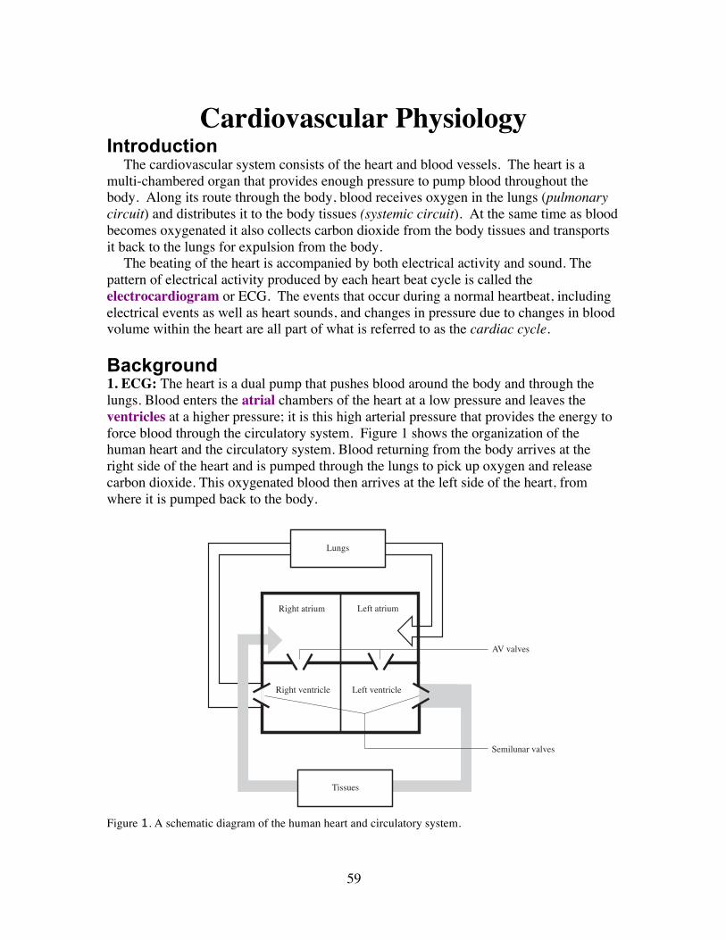
59
Cardiovascular Physiology Introduction
The cardiovascular system consists of the heart and blood vessels. The heart is a multi-chambered organ that provides enough pressure to pump blood throughout the body. Along its route through the body, blood receives oxygen in the lungs (pulmonary circuit) and distributes it to the body tissues (systemic circuit). At the same time as blood becomes oxygenated it also collects carbon dioxide from the body tissues and transports it back to the lungs for expulsion from the body.
The beating of the heart is accompanied by both electrical activity and sound. The pattern of electrical activity produced by each heart beat cycle is called the electrocardiogram or ECG. The events that occur during a normal heartbeat, including electrical events as well as heart sounds, and changes in pressure due to changes in blood volume within the heart are all part of what is referred to as the cardiac cycle.
Background 1. ECG: The heart is a dual pump that pushes blood around the body and through the lungs. Blood enters the atrial chambers of the heart at a low pressure and leaves the ventricles at a higher pressure; it is this high arterial pressure that provides the energy to force blood through the circulatory system. Figure 1 shows the organization of the human heart and the circulatory system. Blood returning from the body arrives at the right side of the heart and is pumped through the lungs to pick up oxygen and release carbon dioxide. This oxygenated blood then arrives at the left side of the heart, from where it is pumped back to the body.
Figure 1. A schematic diagram of the human heart and circulatory system.
Lungs
Right atrium Left atrium
Right ventricle Left ventricle
Tissues
AV valves
Semilunar valves
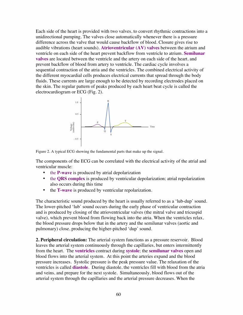
60
Each side of the heart is provided with two valves, to convert rhythmic contractions into a unidirectional pumping. The valves close automatically whenever there is a pressure difference across the valve that would cause backflow of blood. Closure gives rise to audible vibrations (heart sounds). Atrioventricular (AV) valves between the atrium and ventricle on each side of the heart prevent backflow from ventricle to atrium. Semilunar valves are located between the ventricle and the artery on each side of the heart, and prevent backflow of blood from artery to ventricle. The cardiac cycle involves a sequential contraction of the atria and the ventricles. The combined electrical activity of the different myocardial cells produces electrical currents that spread through the body fluids. These currents are large enough to be detected by recording electrodes placed on the skin. The regular pattern of peaks produced by each heart beat cycle is called the electrocardiogram or ECG (Fig. 2).
Figure 2. A typical ECG showing the fundamental parts that make up the signal.
The components of the ECG can be correlated with the electrical activity of the atrial and ventricular muscle:
• the P-wave is produced by atrial depolarization • the QRS complex is produced by ventricular depolarization; atrial repolarization
also occurs during this time • the T-wave is produced by ventricular repolarization.
The characteristic sound produced by the heart is usually referred to as a ‘lub-dup’ sound. The lower-pitched ‘lub’ sound occurs during the early phase of ventricular contraction and is produced by closing of the atrioventricular valves (the mitral valve and tricuspid valve), which prevent blood from flowing back into the atria. When the ventricles relax, the blood pressure drops below that in the artery and the semilunar valves (aortic and pulmonary) close, producing the higher-pitched ‘dup’ sound. 2. Peripheral circulation: The arterial system functions as a pressure reservoir. Blood leaves the arterial system continuously through the capillaries, but enters intermittently from the heart. The ventricles contract during systole; the semilunar valves open and blood flows into the arterial system. At this point the arteries expand and the blood pressure increases. Systolic pressure is the peak pressure value. The relaxation of the ventricles is called diastole. During diastole, the ventricles fill with blood from the atria and veins, and prepare for the next systole. Simultaneously, blood flows out of the arterial system through the capillaries and the arterial pressure decreases. When the
– 0.5
0.5
1.0
Vo
ltage
(mill
ivol
ts) P
R
T
QS
Time
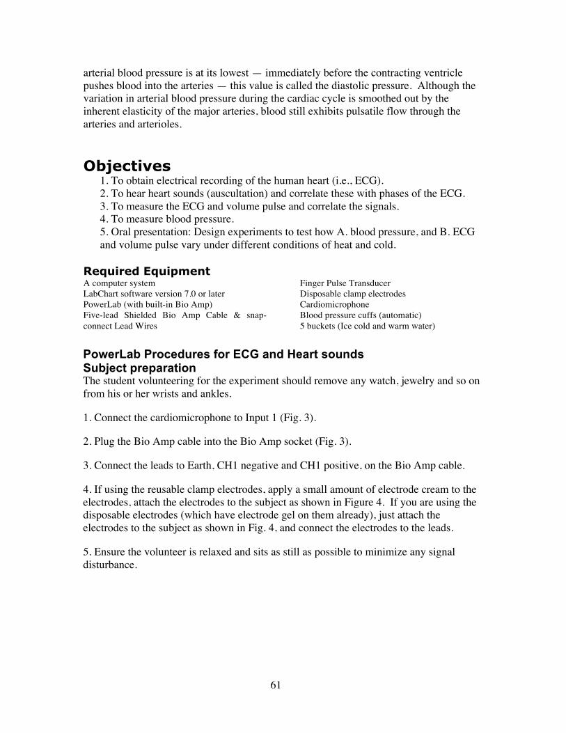
61
arterial blood pressure is at its lowest — immediately before the contracting ventricle pushes blood into the arteries — this value is called the diastolic pressure. Although the variation in arterial blood pressure during the cardiac cycle is smoothed out by the inherent elasticity of the major arteries, blood still exhibits pulsatile flow through the arteries and arterioles. Objectives
1. To obtain electrical recording of the human heart (i.e., ECG). 2. To hear heart sounds (auscultation) and correlate these with phases of the ECG. 3. To measure the ECG and volume pulse and correlate the signals. 4. To measure blood pressure. 5. Oral presentation: Design experiments to test how A. blood pressure, and B. ECG and volume pulse vary under different conditions of heat and cold.
Required Equipment A computer system LabChart software version 7.0 or later PowerLab (with built-in Bio Amp) Five-lead Shielded Bio Amp Cable & snap-connect Lead Wires
Finger Pulse Transducer Disposable clamp electrodes Cardiomicrophone Blood pressure cuffs (automatic) 5 buckets (Ice cold and warm water)
PowerLab Procedures for ECG and Heart sounds Subject preparation The student volunteering for the experiment should remove any watch, jewelry and so on from his or her wrists and ankles.
1. Connect the cardiomicrophone to Input 1 (Fig. 3).
2. Plug the Bio Amp cable into the Bio Amp socket (Fig. 3).
3. Connect the leads to Earth, CH1 negative and CH1 positive, on the Bio Amp cable.
4. If using the reusable clamp electrodes, apply a small amount of electrode cream to the electrodes, attach the electrodes to the subject as shown in Figure 4. If you are using the disposable electrodes (which have electrode gel on them already), just attach the electrodes to the subject as shown in Fig. 4, and connect the electrodes to the leads.
5. Ensure the volunteer is relaxed and sits as still as possible to minimize any signal disturbance.
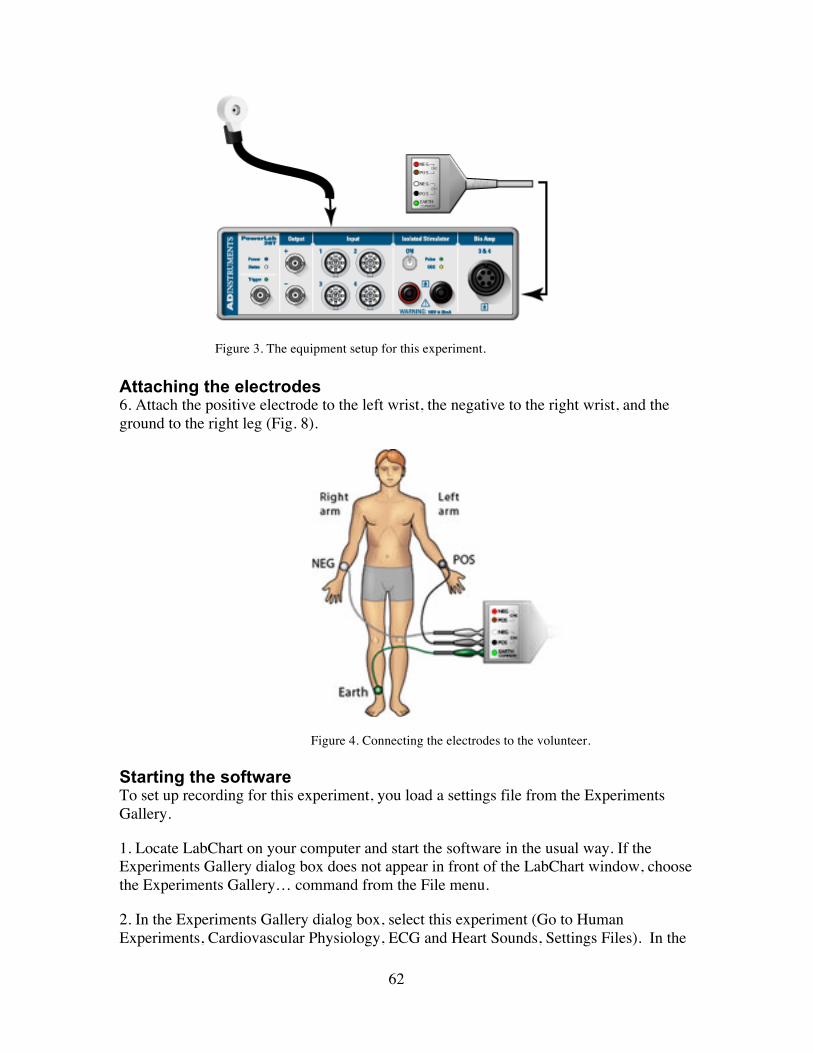
62
Figure 3. The equipment setup for this experiment. Attaching the electrodes 6. Attach the positive electrode to the left wrist, the negative to the right wrist, and the ground to the right leg (Fig. 8).
Figure 4. Connecting the electrodes to the volunteer. Starting the software To set up recording for this experiment, you load a settings file from the Experiments Gallery.
1. Locate LabChart on your computer and start the software in the usual way. If the Experiments Gallery dialog box does not appear in front of the LabChart window, choose the Experiments Gallery… command from the File menu.
2. In the Experiments Gallery dialog box, select this experiment (Go to Human Experiments, Cardiovascular Physiology, ECG and Heart Sounds, Settings Files). In the
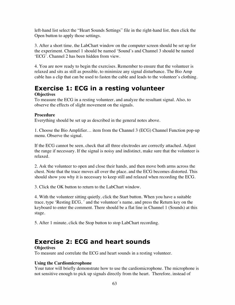
63
left-hand list select the “Heart Sounds Settings” file in the right-hand list, then click the Open button to apply those settings.
3. After a short time, the LabChart window on the computer screen should be set up for the experiment. Channel 1 should be named ‘Sound’s and Channel 3 should be named ‘ECG’. Channel 2 has been hidden from view.
4. You are now ready to begin the exercises. Remember to ensure that the volunteer is relaxed and sits as still as possible, to minimize any signal disturbance. The Bio Amp cable has a clip that can be used to fasten the cable and leads to the volunteer’s clothing.
Exercise 1: ECG in a resting volunteer Objectives To measure the ECG in a resting volunteer, and analyze the resultant signal. Also, to observe the effects of slight movement on the signals.
Procedure Everything should be set up as described in the general notes above.
1. Choose the Bio Amplifier… item from the Channel 3 (ECG) Channel Function pop-up menu. Observe the signal.
If the ECG cannot be seen, check that all three electrodes are correctly attached. Adjust the range if necessary. If the signal is noisy and indistinct, make sure that the volunteer is relaxed.
2. Ask the volunteer to open and close their hands, and then move both arms across the chest. Note that the trace moves all over the place, and the ECG becomes distorted. This should show you why it is necessary to keep still and relaxed when recording the ECG.
3. Click the OK button to return to the LabChart window.
4. With the volunteer sitting quietly, click the Start button. When you have a suitable trace, type ‘Resting ECG, ’ and the volunteer’s name, and press the Return key on the keyboard to enter the comment. There should be a flat line in Channel 1 (Sounds) at this stage.
5. After 1 minute, click the Stop button to stop LabChart recording.
Exercise 2: ECG and heart sounds Objectives To measure and correlate the ECG and heart sounds in a resting volunteer.
Using the Cardiomicrophone Your tutor will briefly demonstrate how to use the cardiomicrophone. The microphone is not sensitive enough to pick up signals directly from the heart. Therefore, instead of
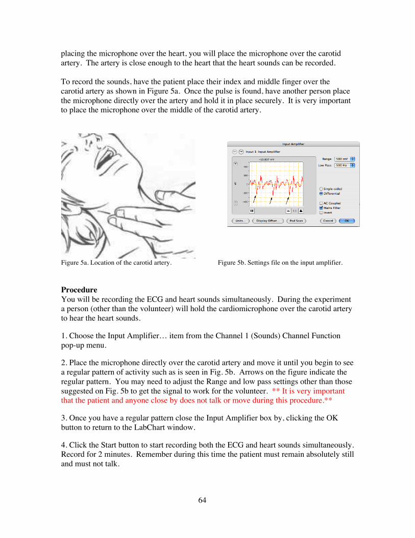
64
placing the microphone over the heart, you will place the microphone over the carotid artery. The artery is close enough to the heart that the heart sounds can be recorded. To record the sounds, have the patient place their index and middle finger over the carotid artery as shown in Figure 5a. Once the pulse is found, have another person place the microphone directly over the artery and hold it in place securely. It is very important to place the microphone over the middle of the carotid artery.
Figure 5a. Location of the carotid artery. Figure 5b. Settings file on the input amplifier. Procedure You will be recording the ECG and heart sounds simultaneously. During the experiment a person (other than the volunteer) will hold the cardiomicrophone over the carotid artery to hear the heart sounds.
1. Choose the Input Amplifier… item from the Channel 1 (Sounds) Channel Function pop-up menu.
2. Place the microphone directly over the carotid artery and move it until you begin to see a regular pattern of activity such as is seen in Fig. 5b. Arrows on the figure indicate the regular pattern. You may need to adjust the Range and low pass settings other than those suggested on Fig. 5b to get the signal to work for the volunteer. ** It is very important that the patient and anyone close by does not talk or move during this procedure.**
3. Once you have a regular pattern close the Input Amplifier box by, clicking the OK button to return to the LabChart window.
4. Click the Start button to start recording both the ECG and heart sounds simultaneously. Record for 2 minutes. Remember during this time the patient must remain absolutely still and must not talk.
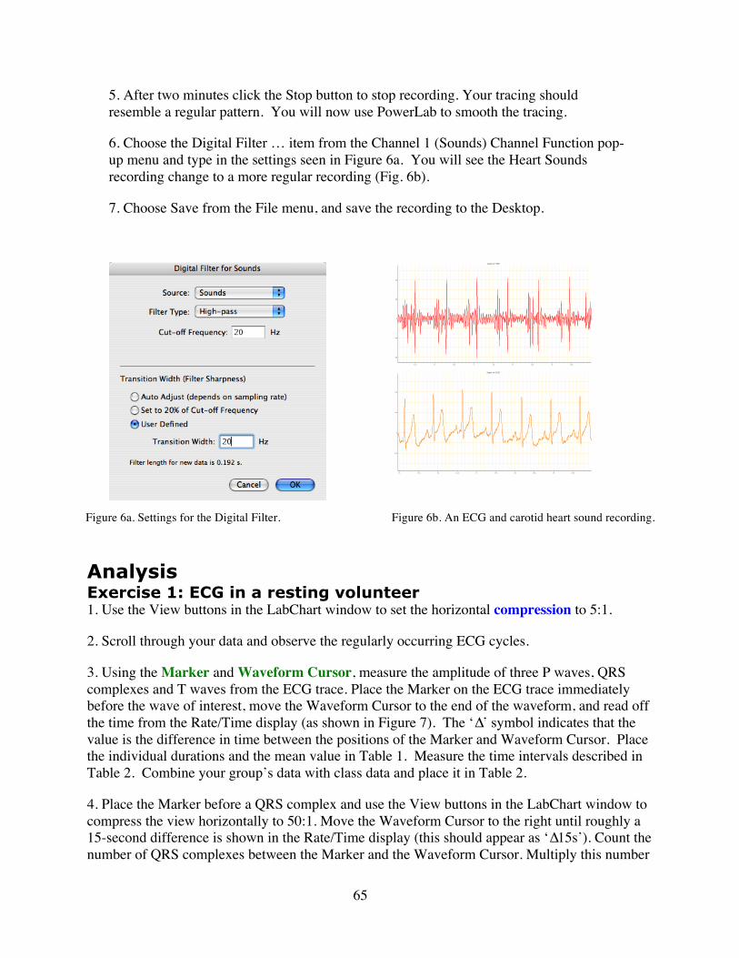
65
5. After two minutes click the Stop button to stop recording. Your tracing should resemble a regular pattern. You will now use PowerLab to smooth the tracing.
6. Choose the Digital Filter … item from the Channel 1 (Sounds) Channel Function pop-up menu and type in the settings seen in Figure 6a. You will see the Heart Sounds recording change to a more regular recording (Fig. 6b).
7. Choose Save from the File menu, and save the recording to the Desktop.
Figure 6a. Settings for the Digital Filter. Figure 6b. An ECG and carotid heart sound recording.
Analysis Exercise 1: ECG in a resting volunteer 1. Use the View buttons in the LabChart window to set the horizontal compression to 5:1.
2. Scroll through your data and observe the regularly occurring ECG cycles.
3. Using the Marker and Waveform Cursor, measure the amplitude of three P waves, QRS complexes and T waves from the ECG trace. Place the Marker on the ECG trace immediately before the wave of interest, move the Waveform Cursor to the end of the waveform, and read off the time from the Rate/Time display (as shown in Figure 7). The ‘∆’ symbol indicates that the value is the difference in time between the positions of the Marker and Waveform Cursor. Place the individual durations and the mean value in Table 1. Measure the time intervals described in Table 2. Combine your group’s data with class data and place it in Table 2.
4. Place the Marker before a QRS complex and use the View buttons in the LabChart window to compress the view horizontally to 50:1. Move the Waveform Cursor to the right until roughly a 15-second difference is shown in the Rate/Time display (this should appear as ‘∆15s’). Count the number of QRS complexes between the Marker and the Waveform Cursor. Multiply this number
Zoom of “HS”
9.598.587.576.565.5
-40
-20
0
20
40
!Zoom of “ECG”
19.51918.51817.51716.51615.515
-0.2
0
0.2
0.4
!
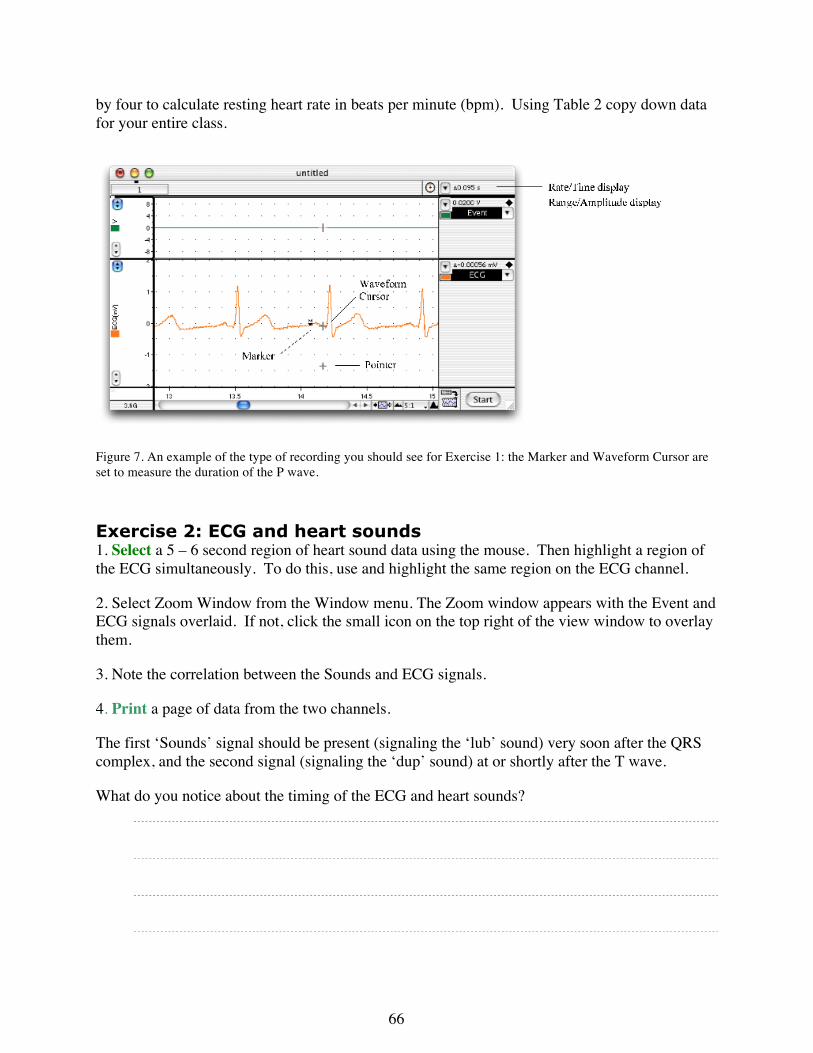
66
by four to calculate resting heart rate in beats per minute (bpm). Using Table 2 copy down data for your entire class.
Figure 7. An example of the type of recording you should see for Exercise 1: the Marker and Waveform Cursor are set to measure the duration of the P wave.
Exercise 2: ECG and heart sounds 1. Select a 5 – 6 second region of heart sound data using the mouse. Then highlight a region of the ECG simultaneously. To do this, use and highlight the same region on the ECG channel.
2. Select Zoom Window from the Window menu. The Zoom window appears with the Event and ECG signals overlaid. If not, click the small icon on the top right of the view window to overlay them.
3. Note the correlation between the Sounds and ECG signals.
4. Print a page of data from the two channels.
The first ‘Sounds’ signal should be present (signaling the ‘lub’ sound) very soon after the QRS complex, and the second signal (signaling the ‘dup’ sound) at or shortly after the T wave.
What do you notice about the timing of the ECG and heart sounds?
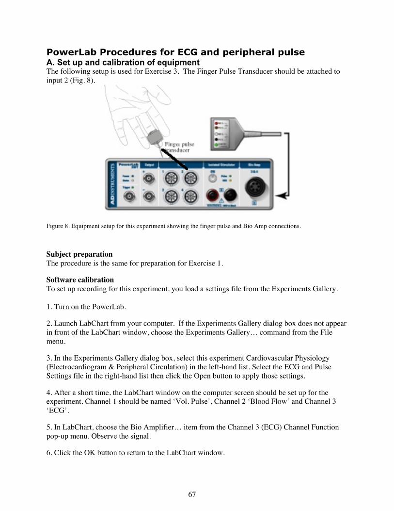
67
PowerLab Procedures for ECG and peripheral pulse A. Set up and calibration of equipment The following setup is used for Exercise 3. The Finger Pulse Transducer should be attached to input 2 (Fig. 8).
Figure 8. Equipment setup for this experiment showing the finger pulse and Bio Amp connections.
Subject preparation The procedure is the same for preparation for Exercise 1.
Software calibration To set up recording for this experiment, you load a settings file from the Experiments Gallery. 1. Turn on the PowerLab.
2. Launch LabChart from your computer. If the Experiments Gallery dialog box does not appear in front of the LabChart window, choose the Experiments Gallery… command from the File menu.
3. In the Experiments Gallery dialog box, select this experiment Cardiovascular Physiology (Electrocardiogram & Peripheral Circulation) in the left-hand list. Select the ECG and Pulse Settings file in the right-hand list then click the Open button to apply those settings.
4. After a short time, the LabChart window on the computer screen should be set up for the experiment. Channel 1 should be named ‘Vol. Pulse’, Channel 2 ‘Blood Flow’ and Channel 3 ‘ECG’.
5. In LabChart, choose the Bio Amplifier… item from the Channel 3 (ECG) Channel Function pop-up menu. Observe the signal.
6. Click the OK button to return to the LabChart window.
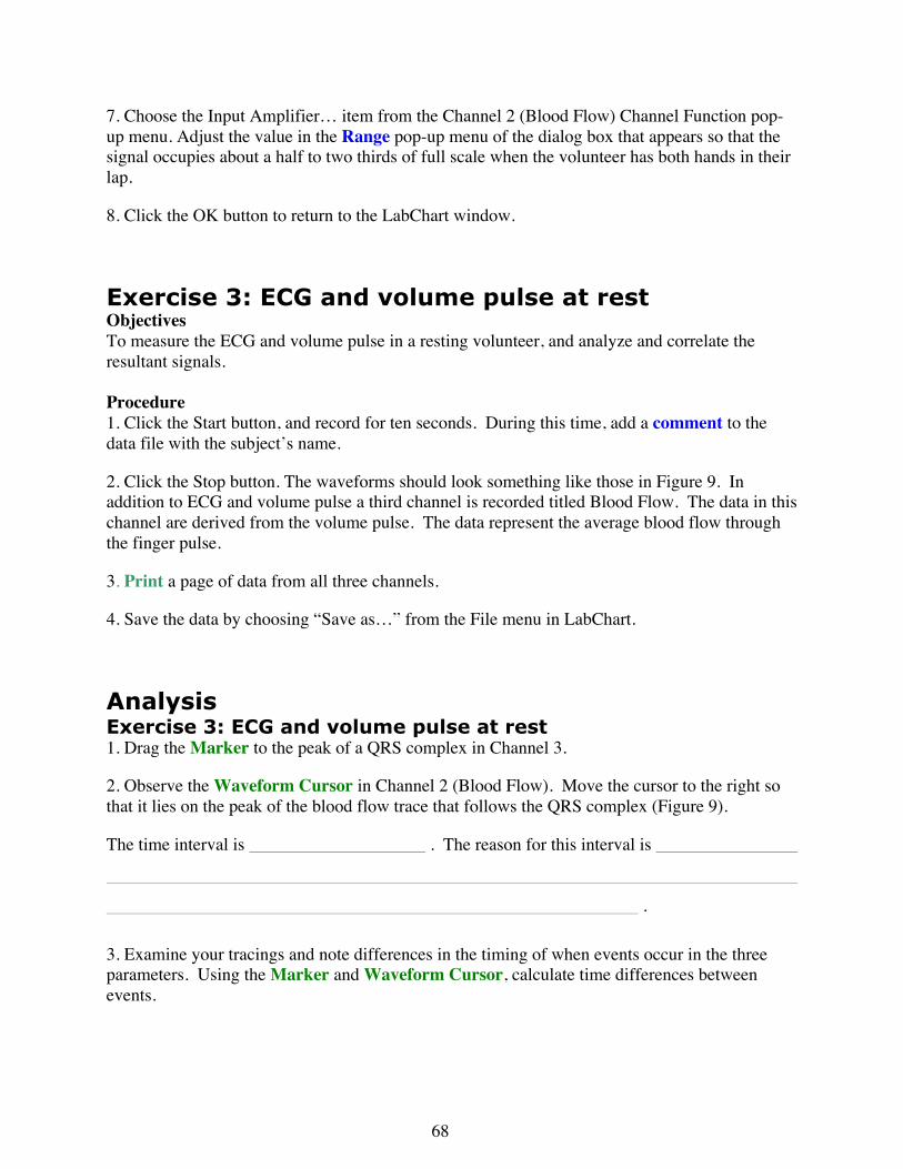
68
7. Choose the Input Amplifier… item from the Channel 2 (Blood Flow) Channel Function pop-up menu. Adjust the value in the Range pop-up menu of the dialog box that appears so that the signal occupies about a half to two thirds of full scale when the volunteer has both hands in their lap.
8. Click the OK button to return to the LabChart window.
Exercise 3: ECG and volume pulse at rest Objectives To measure the ECG and volume pulse in a resting volunteer, and analyze and correlate the resultant signals. Procedure 1. Click the Start button, and record for ten seconds. During this time, add a comment to the data file with the subject’s name.
2. Click the Stop button. The waveforms should look something like those in Figure 9. In addition to ECG and volume pulse a third channel is recorded titled Blood Flow. The data in this channel are derived from the volume pulse. The data represent the average blood flow through the finger pulse.
3. Print a page of data from all three channels.
4. Save the data by choosing “Save as…” from the File menu in LabChart.
Analysis Exercise 3: ECG and volume pulse at rest 1. Drag the Marker to the peak of a QRS complex in Channel 3.
2. Observe the Waveform Cursor in Channel 2 (Blood Flow). Move the cursor to the right so that it lies on the peak of the blood flow trace that follows the QRS complex (Figure 9).
The time interval is . The reason for this interval is
.
3. Examine your tracings and note differences in the timing of when events occur in the three parameters. Using the Marker and Waveform Cursor, calculate time differences between events.
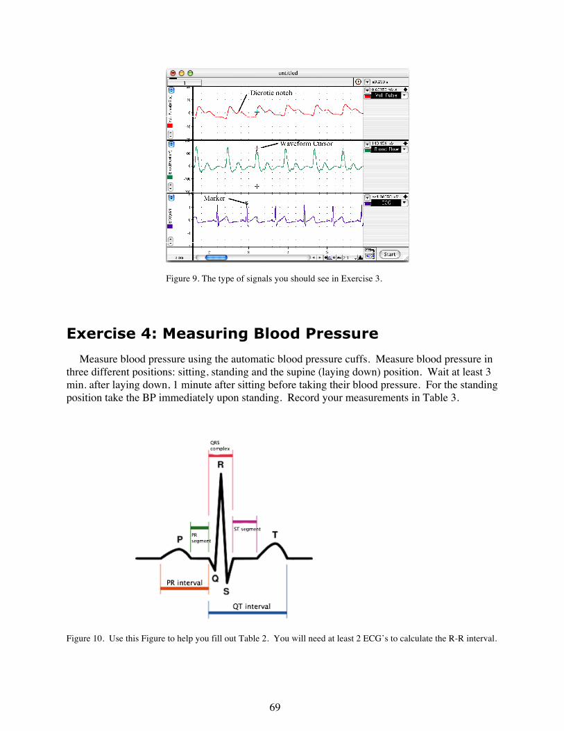
69
Figure 9. The type of signals you should see in Exercise 3.
Exercise 4: Measuring Blood Pressure Measure blood pressure using the automatic blood pressure cuffs. Measure blood pressure in
three different positions: sitting, standing and the supine (laying down) position. Wait at least 3 min. after laying down, 1 minute after sitting before taking their blood pressure. For the standing position take the BP immediately upon standing. Record your measurements in Table 3.
Figure 10. Use this Figure to help you fill out Table 2. You will need at least 2 ECG’s to calculate the R-R interval.
!
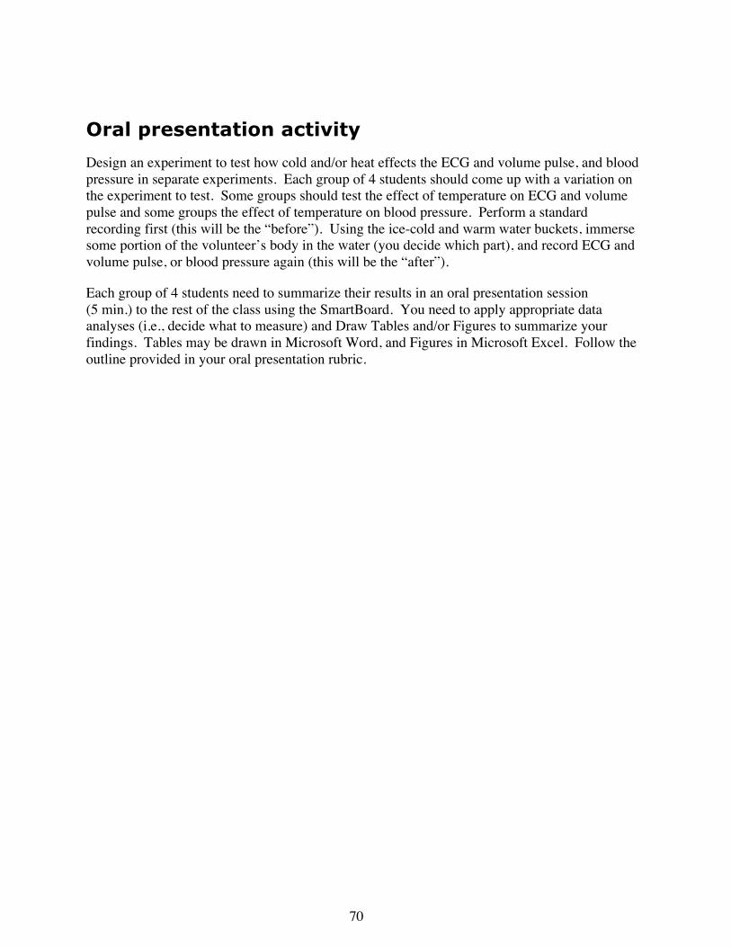
70
Oral presentation activity Design an experiment to test how cold and/or heat effects the ECG and volume pulse, and blood pressure in separate experiments. Each group of 4 students should come up with a variation on the experiment to test. Some groups should test the effect of temperature on ECG and volume pulse and some groups the effect of temperature on blood pressure. Perform a standard recording first (this will be the “before”). Using the ice-cold and warm water buckets, immerse some portion of the volunteer’s body in the water (you decide which part), and record ECG and volume pulse, or blood pressure again (this will be the “after”).
Each group of 4 students need to summarize their results in an oral presentation session (5 min.) to the rest of the class using the SmartBoard. You need to apply appropriate data analyses (i.e., decide what to measure) and Draw Tables and/or Figures to summarize your findings. Tables may be drawn in Microsoft Word, and Figures in Microsoft Excel. Follow the outline provided in your oral presentation rubric.
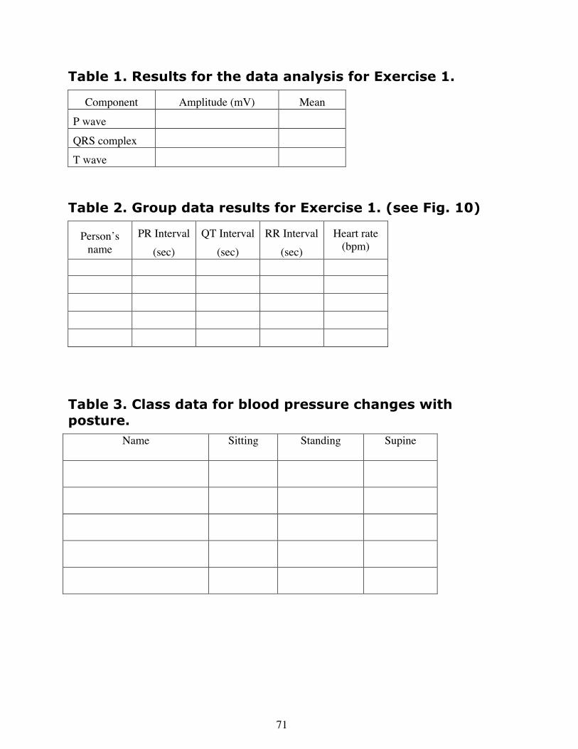
71
Table 1. Results for the data analysis for Exercise 1.
Component Amplitude (mV) Mean
P wave
QRS complex
T wave
Table 2. Group data results for Exercise 1. (see Fig. 10)
Person’s name
PR Interval (sec)
QT Interval (sec)
RR Interval (sec)
Heart rate (bpm)
Table 3. Class data for blood pressure changes with posture.
Name
Sitting Standing Supine
72
Study Questions 1. What can you say about the amplitude of the various waves in different cardiac cycles?
2. The P wave and the QRS complex represent depolarization of the atrial and ventricular muscle respectively. Why does the QRS complex have the largest amplitude?
3. The range for a normal human resting heart rate is 60 to 90 bpm. A trained athlete could have a resting heart rate of 45 to 60 bpm. Why might a very fit person have a slower heart rate than someone of average fitness?
4. Are the amplitudes and durations of the various waves in different individuals similar or very different? If there are differences what might cause them?

73
5. Explain why ventricular contraction (systole) and the ‘lub’ sound occur immediately after the QRS complex.
6. Explain why ventricular relaxation (diastole) and the ‘dub’ sound occur after the T wave.
7. What happened to the blood pressure value when the volunteer was standing? Lying down? Explain the physiological mechanism responsible for this effect.

74
Physiology of the in situ amphibian Heart In this experiment, you will explore the basic principles of cardiac muscle physiology, including contraction force, an electrocardiogram (ECG), the effect of drugs on the heart, and conduction blockade. You will examine the frog heart in situ. Written by staff of ADInstruments. Background Studies of isolated organs were pioneered in the late 19th century when scientists such as Sidney Ringer (1835-1910) developed perfusion solutions (such as Ringer's solution) based upon the composition of the extracellular fluid that could sustain an organ isolated from a pithed animal. A classic example of an isolated organ preparation is the frog heart. It will continue to beat in situ for several hours, during which basic cardiac functions can be investigated. The heart is made up of cardiac muscle. Cardiac muscle is similar to skeletal (striated) muscle, but exhibits some special properties, the most important of which is rhythmicity. All cardiac muscle cells have the inherent ability to depolarize and repolarize. These action potentials spread to adjacent cells via gap junctions that allow ions to move; thus current flows from cell to cell. In this way the atria and the ventricles behave as electrical syncytia. These spontaneous cycles of depolarization and repolarization occur in rhythmic fashion, giving rise to an intrinsic, regular heartbeat. In the intact, normal heart, the heart rate is determined by the group of cells – the pacemaker cells – that undergo the fastest depolarization/repolarization cycle. In the mammalian heart, the pacemaker cells are located in the sinoatrial (SA) node. In the frog heart, the sinus venosus is the functional equivalent of the mammalian SA node (Figure 1).
Figure 1. Ventral and Dorsal Views of the Frog Heart
As well as cell-to-cell current flow, there is a specialized conduction pathway. This provides the only electrical connection between the atria and ventricles – the AV node. Although there are pacemaker cells here, conduction is much slower than it is through either atrial or ventricular muscle. This allows the depolarization of the atria (and thereby atrial contraction) to be completed before the ventricles depolarize and contract. From the AV node, the action potentials travel at high speeds (1 m/s in the mammalian heart) down the ventricular septum in the Bundle of His and then along the left and right bundles to enter the Purkinje network that penetrates the entire ventricular muscle. Conduction here is very fast (5 m/s in the mammalian heart) so ventricular depolarization is very rapid, and the ventricular muscle contracts as a whole.
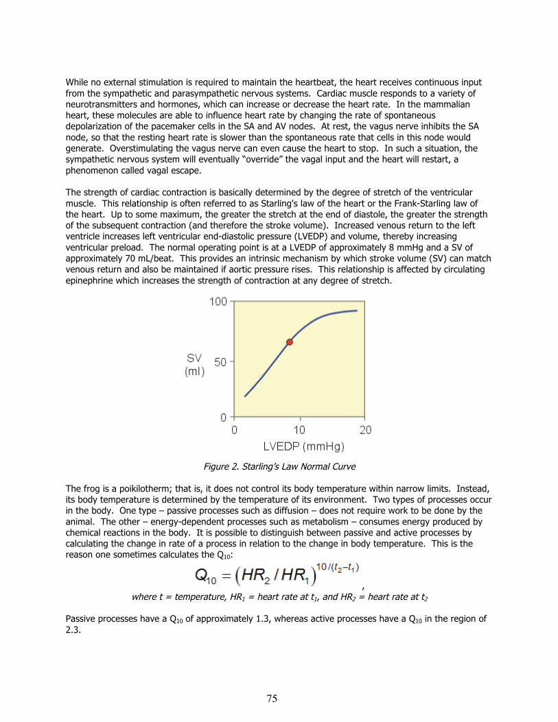
75
While no external stimulation is required to maintain the heartbeat, the heart receives continuous input from the sympathetic and parasympathetic nervous systems. Cardiac muscle responds to a variety of neurotransmitters and hormones, which can increase or decrease the heart rate. In the mammalian heart, these molecules are able to influence heart rate by changing the rate of spontaneous depolarization of the pacemaker cells in the SA and AV nodes. At rest, the vagus nerve inhibits the SA node, so that the resting heart rate is slower than the spontaneous rate that cells in this node would generate. Overstimulating the vagus nerve can even cause the heart to stop. In such a situation, the sympathetic nervous system will eventually “override” the vagal input and the heart will restart, a phenomenon called vagal escape. The strength of cardiac contraction is basically determined by the degree of stretch of the ventricular muscle. This relationship is often referred to as Starling's law of the heart or the Frank-Starling law of the heart. Up to some maximum, the greater the stretch at the end of diastole, the greater the strength of the subsequent contraction (and therefore the stroke volume). Increased venous return to the left ventricle increases left ventricular end-diastolic pressure (LVEDP) and volume, thereby increasing ventricular preload. The normal operating point is at a LVEDP of approximately 8 mmHg and a SV of approximately 70 mL/beat. This provides an intrinsic mechanism by which stroke volume (SV) can match venous return and also be maintained if aortic pressure rises. This relationship is affected by circulating epinephrine which increases the strength of contraction at any degree of stretch.
Figure 2. Starling’s Law Normal Curve
The frog is a poikilotherm; that is, it does not control its body temperature within narrow limits. Instead, its body temperature is determined by the temperature of its environment. Two types of processes occur in the body. One type – passive processes such as diffusion – does not require work to be done by the animal. The other – energy-dependent processes such as metabolism – consumes energy produced by chemical reactions in the body. It is possible to distinguish between passive and active processes by calculating the change in rate of a process in relation to the change in body temperature. This is the reason one sometimes calculates the Q10:
, where t = temperature, HR1 = heart rate at t1, and HR2 = heart rate at t2
Passive processes have a Q10 of approximately 1.3, whereas active processes have a Q10 in the region of 2.3.

76
Note that the frog heart differs from the mammalian heart in that it has three chambers rather than four. The pacemaker cells are located in the sinus venosus that receives deoxygenated blood from the veins that drain most of the body organs and empties this into the right atrium. Oxygenated blood from the lungs returns to the left atrium. The single ventricle receives blood from both atria and pumps it out through one large artery – the truncus arteriosus. However, the anatomical organization of the ventricle and the outflow tract is such that there is little mixing of the two pools of blood. The consequence of this is that oxygenated blood is delivered to the brain and most tissues, whereas the deoxygenated blood flows to the lungs and skin (Figure 3). Frogs exchange gases and water through their skin.
Figure 3. Internal Features of the Frog Heart Required Equipment
• LabChart 7 software • PowerLab Data Acquisition Unit with a
Bio Amp • Bridge Pod • Force Transducer • Small weight between 1-20 grams • Ring Stand • Manipulator/Micropositioner and clamps • 5 Lead Shielded Bio Amp Cable • Shielded Lead Wires (3 Alligator Clips) • Strong thread • Barbless hook • Pasteur pipette • Thermometer • Syringe • Dissection tools:
o Sharp scissors o Blunt probe o Dissection tray with wax or pad o Dissection pins • Solutions: o Frog Ringer’s – room
temperature o Frog Ringer’s – cold (in a 4oC
water bath) o Frog Ringer’s – warm (in a 37oC
water bath) o Acetylcholine (0.1 mg/mL) o Epinephrine (0.1 mg/mL) o Pilocarpine (0.2 mg/mL) o Atropine (1.0 mg/mL) o Nicotine (1 and 3 drops/20 ml)
Procedure Equipment Setup and Calibration 1. Make sure the PowerLab is turned off and the USB cable is connected to the computer.
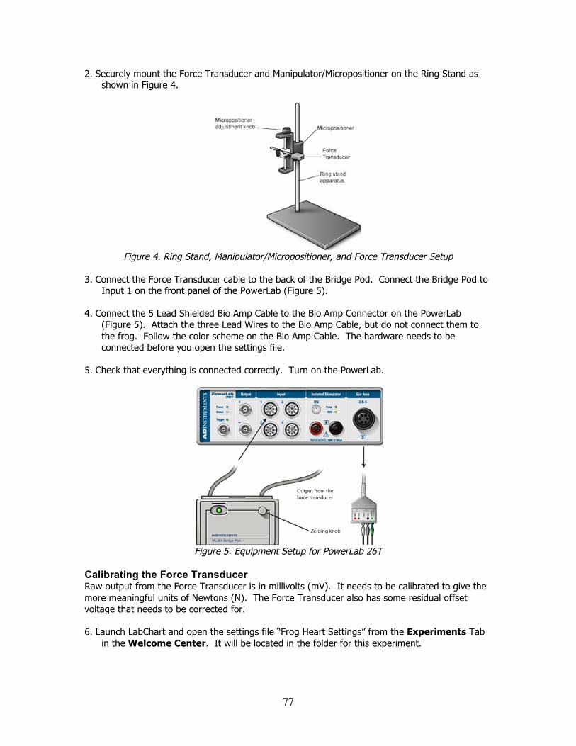
77
2. Securely mount the Force Transducer and Manipulator/Micropositioner on the Ring Stand as shown in Figure 4.
Figure 4. Ring Stand, Manipulator/Micropositioner, and Force Transducer Setup
3. Connect the Force Transducer cable to the back of the Bridge Pod. Connect the Bridge Pod to
Input 1 on the front panel of the PowerLab (Figure 5).
4. Connect the 5 Lead Shielded Bio Amp Cable to the Bio Amp Connector on the PowerLab (Figure 5). Attach the three Lead Wires to the Bio Amp Cable, but do not connect them to the frog. Follow the color scheme on the Bio Amp Cable. The hardware needs to be connected before you open the settings file.
5. Check that everything is connected correctly. Turn on the PowerLab.
Figure 5. Equipment Setup for PowerLab 26T
Calibrating the Force Transducer Raw output from the Force Transducer is in millivolts (mV). It needs to be calibrated to give the more meaningful units of Newtons (N). The Force Transducer also has some residual offset voltage that needs to be corrected for. 6. Launch LabChart and open the settings file “Frog Heart Settings” from the Experiments Tab
in the Welcome Center. It will be located in the folder for this experiment.
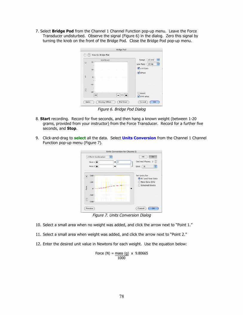
78
7. Select Bridge Pod from the Channel 1 Channel Function pop-up menu. Leave the Force Transducer undisturbed. Observe the signal (Figure 6) in the dialog. Zero this signal by turning the knob on the front of the Bridge Pod. Close the Bridge Pod pop-up menu.
Figure 6. Bridge Pod Dialog
8. Start recording. Record for five seconds, and then hang a known weight (between 1-20
grams, provided from your instructor) from the Force Transducer. Record for a further five seconds, and Stop.
9. Click-and-drag to select all the data. Select Units Conversion from the Channel 1 Channel Function pop-up menu (Figure 7).
Figure 7. Units Conversion Dialog
10. Select a small area when no weight was added, and click the arrow next to “Point 1.”
11. Select a small area when weight was added, and click the arrow next to “Point 2.”
12. Enter the desired unit value in Newtons for each weight. Use the equation below:
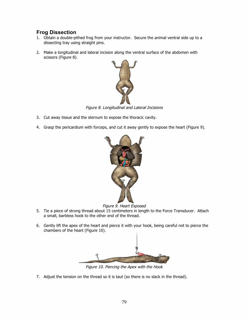
79
Frog Dissection 1. Obtain a double-pithed frog from your instructor. Secure the animal ventral side up to a
dissecting tray using straight pins. 2. Make a longitudinal and lateral incision along the ventral surface of the abdomen with
scissors (Figure 8).
Figure 8. Longitudinal and Lateral Incisions
3. Cut away tissue and the sternum to expose the thoracic cavity. 4. Grasp the pericardium with forceps, and cut it away gently to expose the heart (Figure 9).
Figure 9. Heart Exposed
5. Tie a piece of strong thread about 15 centimeters in length to the Force Transducer. Attach a small, barbless hook to the other end of the thread.
6. Gently lift the apex of the heart and pierce it with your hook, being careful not to pierce the
chambers of the heart (Figure 10).
Figure 10. Piercing the Apex with the Hook
7. Adjust the tension on the thread so it is taut (so there is no slack in the thread).
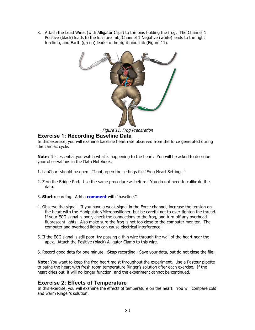
80
8. Attach the Lead Wires (with Alligator Clips) to the pins holding the frog. The Channel 1 Positive (black) leads to the left forelimb, Channel 1 Negative (white) leads to the right forelimb, and Earth (green) leads to the right hindlimb (Figure 11).
Figure 11. Frog Preparation
Exercise 1: Recording Baseline Data In this exercise, you will examine baseline heart rate observed from the force generated during the cardiac cycle. Note: It is essential you watch what is happening to the heart. You will be asked to describe your observations in the Data Notebook. 1. LabChart should be open. If not, open the settings file “Frog Heart Settings.”
2. Zero the Bridge Pod. Use the same procedure as before. You do not need to calibrate the data.
3. Start recording. Add a comment with “baseline.”
4. Observe the signal. If you have a weak signal in the Force channel, increase the tension on the heart with the Manipulator/Micropositioner, but be careful not to over-tighten the thread. If your ECG signal is poor, check the connections to the frog, and turn off any overhead fluorescent lights. Also make sure the frog is not too close to the computer monitor. The computer and overhead lights can cause electrical interference.
5. If the ECG signal is still poor, try passing a thin wire through the wall of the heart near the apex. Attach the Positive (black) Alligator Clamp to this wire.
6. Record good data for one minute. Stop recording. Save your data, but do not close the file.
Note: You want to keep the frog heart moist throughout the experiment. Use a Pasteur pipette to bathe the heart with fresh room temperature Ringer’s solution after each exercise. If the heart dries out, it will no longer function, and the experiment cannot be continued.
Exercise 2: Effects of Temperature In this exercise, you will examine the effects of temperature on the heart. You will compare cold and warm Ringer’s solution.
81
1. Zero the Bridge Pod as before. 2. Measure the temperature of the normal Ringer’s solution. Record the value in Table 2 of the
Data Notebook.
3. Using the same file, Start recording. Add a comment with “exercise 2.” Record baseline data for 1 minute. Do not stop recording until the end of the exercise. 4. Measure the temperature of the warm Ringer’s solution (37°C). Record the value in Table 2 of
the Data Notebook.
5. Using a Pasteur pipette, bathe the heart in warm Ringer’s solution. Add a comment with “warm.” Record for 2 minutes. Pipette out any excess fluid from the peritoneal cavity.
1. Measure the temperature of the cold Ringer’s solution (4°C). Record the value in Table 2 of the Data Notebook.
Bathe the heart in cold Ringer’s solution. Add a comment with “cold.” Record for 2 minutes. . Pipette out any excess fluid from the peritoneal cavity.
2. Stop recording. Bathe the heart in room temperature Ringer’s solution. Wait one minute before moving on to the next exercise.
3. Save your data. Do not close the file.
Exercise 3: Starling’s Law of the Heart In this exercise, you will investigate Starling’s Law. This states strength of cardiac contraction is determined by the degree of stretch of the ventricular muscle. Up to some maximum, the greater the stretch at the end of diastole, the greater the strength of the subsequent contraction. 1. Zero the Bridge Pod as before. Using the same file, Start recording. Add a comment with
“exercise 3.”
2. Record 10 seconds of baseline data.
3. Continue recording. Slowly increase the tension on the heart by about 0.5 millimeters (no more than one millimeter) by turning the Manipulator/Micropositioner knob. Add a comment with “stretch 0.5 mm.” Continue recording for 10 seconds.
Note: You do not need to turn the knob excessively to see a result.
4. Repeat step 3 for a further four lengths. Add a comment appropriate to the stretch length. Be careful not to stretch the heart excessively.
5. Immediately return the Manipulator/Micropositioner to its original position to reduce the tension on the heart.
6. Stop recording. Save your data, but do not close the file.
7. Bathe the heart with normal Ringer’s solution to prevent it from drying out. Wait at least 30 seconds before moving on to the next exercise.
82
Exercise 4: Effects of Drugs In this exercise, you will examine the effects of two neurotransmitters – acetylcholine and epinephrine – on the heart. Then you will examine what happens to the heart when drugs are added. Acetylcholine is released onto the heart by the postganglionic parasympathetic nerves, whereas epinephrine is released into the circulation from the adrenal glands and by postganglionic sympathetic nerves. Pilocarpine stimulates acetylcholine receptors on the heart, and atropine is a plant alkaloid that blocks the muscarinic acetylcholine receptors on the heart. Note: Be sure to apply the drugs in this exercise in the order indicated. Between each step, allow the heart to recover for two minutes and flush with fresh Ringer’s solution, then pipette out the solution. 1. Zero the Bridge Pod as before.
2. Using the same file, Start recording. Add a comment with “exercise 4.” Record 1 minute of baseline data.
3. Using a syringe, apply two or three drops of acetylcholine (0.1 mg/mL) to the heart. Add a comment with “acetylcholine.” Record for two minutes, then Stop recording.
4. Rinse the heart with Ringer’s solution, and allow it to recover for two minutes.
5. Repeat steps 2-4 for epinephrine (0.1 mg/mL). Add an appropriate comment.
6. Repeat steps 2-4 for pilocarpine (0.2 mg/mL). Add an appropriate comment.
7. Repeat steps 2-4 for both the low and high nicotine (1 and 3 mg/mL). Add an appropriate comment.
8. Start recording, and record 1 minute of baseline data.
9. Using a syringe, apply two or three drops of atropine (1 mg/mL) to the heart. Add a comment with “atropine.” Record for 1 minute.
10. Apply two or three drops of acetylcholine to the heart. Add a comment with “acetylcholine.”
11. Record for two minutes. Stop recording. Save your data, but do not close the file.
12. Rinse the heart with Ringer’s solution, and allow the heart to recover for two minutes.
Analysis Exercise 1: Recording Baseline Data 1. Examine the data in the Chart View. Autoscale, if necessary.
2. Use the View Buttons to set the horizontal compression so you can see all the baseline data at once.
3. Select the baseline data from the Heart Rate [Force] channel. Make sure you only select the data trace. If part of the trace is selected without any data, the Data Pad will not display the mean heart rate (Figure 14).
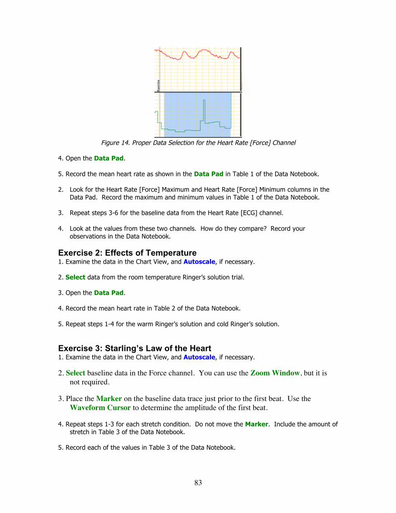
83
Figure 14. Proper Data Selection for the Heart Rate [Force] Channel
4. Open the Data Pad.
5. Record the mean heart rate as shown in the Data Pad in Table 1 of the Data Notebook.
2. Look for the Heart Rate [Force] Maximum and Heart Rate [Force] Minimum columns in the Data Pad. Record the maximum and minimum values in Table 1 of the Data Notebook.
3. Repeat steps 3-6 for the baseline data from the Heart Rate [ECG] channel.
4. Look at the values from these two channels. How do they compare? Record your observations in the Data Notebook.
Exercise 2: Effects of Temperature 1. Examine the data in the Chart View, and Autoscale, if necessary.
2. Select data from the room temperature Ringer’s solution trial.
3. Open the Data Pad.
4. Record the mean heart rate in Table 2 of the Data Notebook.
5. Repeat steps 1-4 for the warm Ringer’s solution and cold Ringer’s solution.
Exercise 3: Starling’s Law of the Heart 1. Examine the data in the Chart View, and Autoscale, if necessary.
2. Select baseline data in the Force channel. You can use the Zoom Window, but it is not required.
3. Place the Marker on the baseline data trace just prior to the first beat. Use the Waveform Cursor to determine the amplitude of the first beat.
4. Repeat steps 1-3 for each stretch condition. Do not move the Marker. Include the amount of stretch in Table 3 of the Data Notebook.
5. Record each of the values in Table 3 of the Data Notebook.

84
1. Use the Heart Rate [ECG] channel to determine the mean heart rate for each stretch condition, using the Data Pad as in Exercise 1. Record these values in Table 3 of the Data Notebook.
Exercise 4: Effects of Drugs 1. Examine the data in the Chart View, and Autoscale, if necessary.
2. For each drug administered, determine the heart rate from the Heart Rate [ECG] channel as in Exercise 1.
3. Record these values in Table 4 of the Data Notebook.
4. Calculate the percent change in heart rate for each drug using the following equation:
!
% change = rate with drug – resting rate( )
resting rate"100
5. Record these values in Table 4 of the Data Notebook.
Data Notebook Exercise 1 Observations a) Describe the heart rate and force seen in your baseline recording of the frog heart cardiac
cycle.
b) Compare the values of heart rate calculated from Force and ECG in Table 1. Are these values the same or different? Why do you think this is the case?
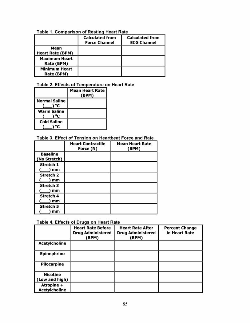
85
Table 1. Comparison of Resting Heart Rate Calculated from
Force Channel Calculated from
ECG Channel Mean
Heart Rate (BPM)
Maximum Heart Rate (BPM)
Minimum Heart Rate (BPM)
Table 2. Effects of Temperature on Heart Rate
Mean Heart Rate (BPM)
Normal Saline (___) oC
Warm Saline (___) oC
Cold Saline (___) oC
Table 3. Effect of Tension on Heartbeat Force and Rate
Heart Contractile Force (N)
Mean Heart Rate (BPM)
Baseline (No Stretch)
Stretch 1 (___) mm
Stretch 2 (___) mm
Stretch 3 (___) mm
Stretch 4 (___) mm
Stretch 5 (___) mm
Table 4. Effects of Drugs on Heart Rate
Heart Rate Before Drug Administered
(BPM)
Heart Rate After Drug Administered
(BPM)
Percent Change in Heart Rate
Acetylcholine
Epinephrine
Pilocarpine
Nicotine (Low and high)
Atropine + Acetylcholine

86
Study Questions 1. Describe the basis for the delay between the atrial and ventricular contractions.
2. How did temperature affect heart rate? What do you suppose is a consequence of
being a poikilotherm?
3. What is Starling’s Law of the Heart? Does your data support this law? How?

87
4. Describe the mechanisms by which the following drugs affect heart rate:
a) acetylcholine:
b) epinephrine:
c) pilocarpine:
d) nicotine:
e) atropine followed by acetylcholine:
88
Respiration
Introduction Ventilation or breathing is responsible for maintaining a continual supply of oxygen for the body and the removal of carbon dioxide. From a simple perspective, during normal breathing inspiration and expiration should follow each other rhythmically, without either phase being unduly prolonged. This basic rhythm of ventilation is established within the respiratory centers of the brain. However, the basic rate and rhythm are not static, but rather vary to alter respiratory rate and depth to meet the physiological demands of the organism. A common misconception is that varying oxygen levels within the system causes changes in ventilation rate. In actuality, oxygen concentration under normal conditions has little to do with determination of respiratory rate. Rather it is the carbon dioxide level that is the determining factor. For example, increased carbon dioxide levels will lead to an accelerated ventilation rate and depth so as to bring carbon dioxide levels back to normal. Conversely, conditions associated with alkalosis and lower than normal carbon dioxide levels will bring about a depressed ventilation rate. Receptors sensitive to the changes in concentrations of carbon dioxide are located in the arterial system and the medulla oblongata of the brain. When excited, these receptors trigger neural reflexes which in turn alter respiratory rate and depth. I. Lung volumes Gas exchange between air and blood occurs in the alveolar air sacs. The efficiency of gas exchange is dependent on ventilation; cyclical breathing movements alternately inflate and deflate the alveolar air sacs. Inspiration fills the alveoli with fresh atmospheric air and expiration removes stale air, which has reduced oxygen and increased carbon dioxide concentrations. Many important aspects of lung function can be determined by measuring airflow and the corresponding changes in lung volume using spirometry. Spirometry allows many components of pulmonary function (Fig. 1) to be visualized, measured and calculated. Respiration consists of repeating cycles of inspiration followed by expiration. During the respiratory cycle, a specific volume of air is drawn into and then expired out of the lungs; this volume is the Tidal Volume (VT). In normal ventilation, the breathing frequency (ƒ) is 12 - 15 respiratory cycles per minute. This value varies with the level of activity. The product of ƒ and VT is the Expired Minute Volume (
!
˙ V E), the amount of air exhaled in one minute of breathing. All these parameters may change according to a person’s height, weight and level of activity.
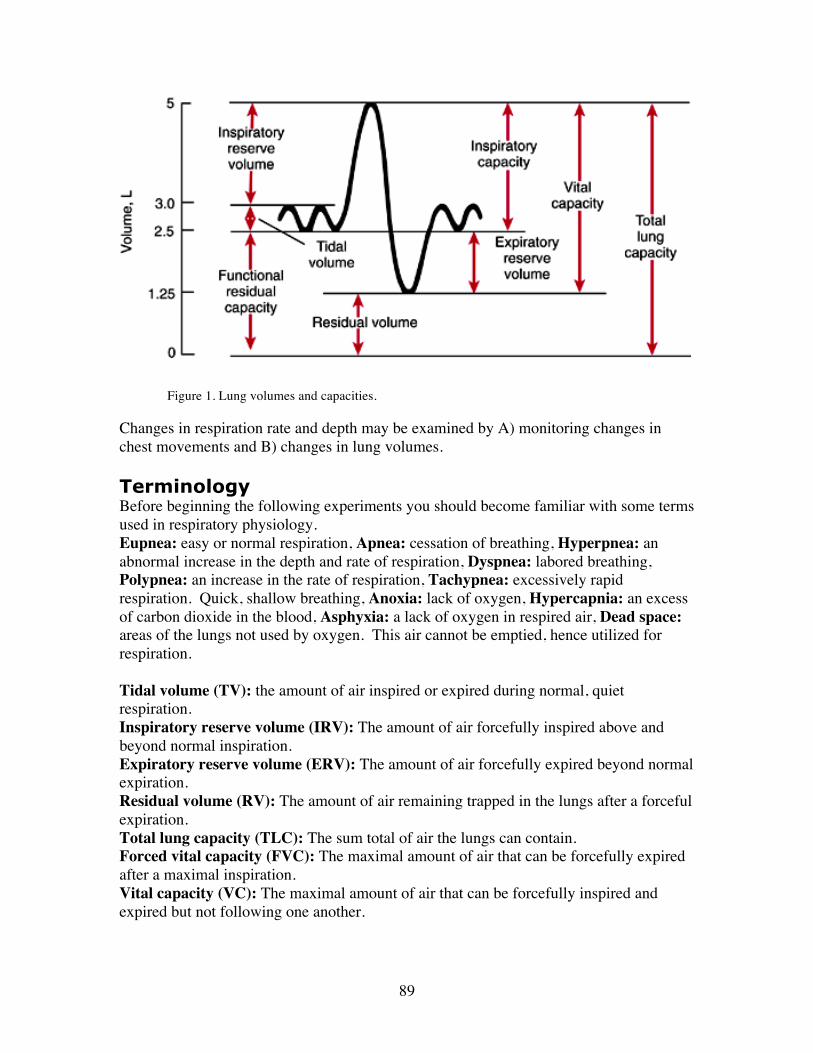
89
Figure 1. Lung volumes and capacities.
Changes in respiration rate and depth may be examined by A) monitoring changes in chest movements and B) changes in lung volumes. Terminology Before beginning the following experiments you should become familiar with some terms used in respiratory physiology. Eupnea: easy or normal respiration, Apnea: cessation of breathing, Hyperpnea: an abnormal increase in the depth and rate of respiration, Dyspnea: labored breathing, Polypnea: an increase in the rate of respiration, Tachypnea: excessively rapid respiration. Quick, shallow breathing, Anoxia: lack of oxygen, Hypercapnia: an excess of carbon dioxide in the blood, Asphyxia: a lack of oxygen in respired air, Dead space: areas of the lungs not used by oxygen. This air cannot be emptied, hence utilized for respiration. Tidal volume (TV): the amount of air inspired or expired during normal, quiet respiration. Inspiratory reserve volume (IRV): The amount of air forcefully inspired above and beyond normal inspiration. Expiratory reserve volume (ERV): The amount of air forcefully expired beyond normal expiration. Residual volume (RV): The amount of air remaining trapped in the lungs after a forceful expiration. Total lung capacity (TLC): The sum total of air the lungs can contain. Forced vital capacity (FVC): The maximal amount of air that can be forcefully expired after a maximal inspiration. Vital capacity (VC): The maximal amount of air that can be forcefully inspired and expired but not following one another.
90
Functional residual capacity (FRC): The amount of air remaining in the lungs after a normal expiration. Inspiratory capacity (IC): The maximal amount of air that can be inspired after a normal expiration. II. Chest movements The principal muscle activity in quiet breathing is rhythmic contraction of the diaphragm, a dome-shaped sheet of muscle that separates the thorax from the abdomen. As contraction of the diaphragm pulls the lower surface of the lungs down, air is inspired. In quiet breathing, expiration is mainly passive, and results from the elastic recoil of the lungs. Rib movements also occur in quiet breathing because of the activity of the intercostal muscles, but are of small amplitude. In forceful breathing, rib movements are obvious, and greatly expand and contract the volume enclosed by the ribcage. In addition, other muscles are recruited. The sternomastoid muscles of the neck assist in raising the sternum in forceful inspiration. Abdominal muscles raise the pressure in the abdomen and push the diaphragm up, providing a powerful expiratory force. Experimental Equipment Macintosh PowerBook LabChart software, version 5.0 PowerLab Spirometer Pod Respiratory flow head (1000 L/min) Disposable filters
Re-useable mouthpieces Nose clip Respiratory belt transducer Medium-sized paper bag
I. PowerLab procedures – Measuring lung capacity Set up and calibration of equipment
A. Connecting the equipment 1. Connect the Spirometer Pod to the Pod Port for Input 1 on the PowerLab.
2. Since the Spirometer Pod is sensitive to temperature and tends to drift during warm-up, we recommend that the PowerLab and Spirometer Pod be turned on for at least 5-10 minutes before use. To prevent temperature drift, place the Spirometer Pod on a shelf or beside the PowerLab, away from the PowerLab power supply to avoid heating.
3. Connect the two plastic tubes from the respiratory flow head to the short pipes on the back of the Spirometer Pod, as shown in Figure 2.
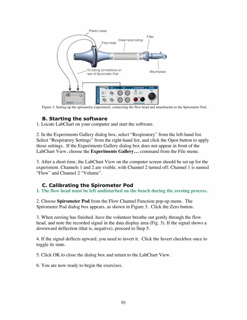
91
Figure 2. Setting up the spirometry experiment: connecting the flow head and attachments to the Spirometer Pod.
B. Starting the software 1. Locate LabChart on your computer and start the software.
2. In the Experiments Gallery dialog box, select “Respiratory” from the left-hand list. Select “Respiratory Settings” from the right-hand list, and click the Open button to apply those settings. If the Experiments Gallery dialog box does not appear in front of the LabChart View, choose the Experiments Gallery… command from the File menu.
3. After a short time, the LabChart View on the computer screen should be set up for the experiment. Channels 1 and 2 are visible, with Channel 2 turned off; Channel 1 is named “Flow” and Channel 2 “Volume”.
C. Calibrating the Spirometer Pod 1. The flow head must be left undisturbed on the bench during the zeroing process.
2. Choose Spirometer Pod from the Flow Channel Function pop-up menu. The Spirometer Pod dialog box appears, as shown in Figure 3. Click the Zero button.
3. When zeroing has finished, have the volunteer breathe out gently through the flow head, and note the recorded signal in the data display area (Fig. 3). If the signal shows a downward deflection (that is, negative), proceed to Step 5.
4. If the signal deflects upward, you need to invert it. Click the Invert checkbox once to toggle its state.
5. Click OK to close the dialog box and return to the LabChart View.
6. You are now ready to begin the exercises.
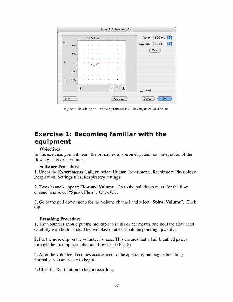
92
Figure 3. The dialog box for the Spirometer Pod, showing an exhaled breath.
Exercise 1: Becoming familiar with the equipment
Objectives In this exercise, you will learn the principles of spirometry, and how integration of the flow signal gives a volume.
Software Procedure 1. Under the Experiments Gallery, select Human Experiments, Respiratory Physiology, Respiration, Settings files, Respiratory settings.
2. Two channels appear: Flow and Volume. Go to the pull down menu for the flow channel and select “Spiro. Flow”. Click OK.
3. Go to the pull down menu for the volume channel and select “Spiro. Volume”. Click OK.
Breathing Procedure 1. The volunteer should put the mouthpiece in his or her mouth, and hold the flow head carefully with both hands. The two plastic tubes should be pointing upwards.
2. Put the nose clip on the volunteer’s nose. This ensures that all air breathed passes through the mouthpiece, filter and flow head (Fig. 8).
3. After the volunteer becomes accustomed to the apparatus and begins breathing normally, you are ready to begin.
4. Click the Start button to begin recording.
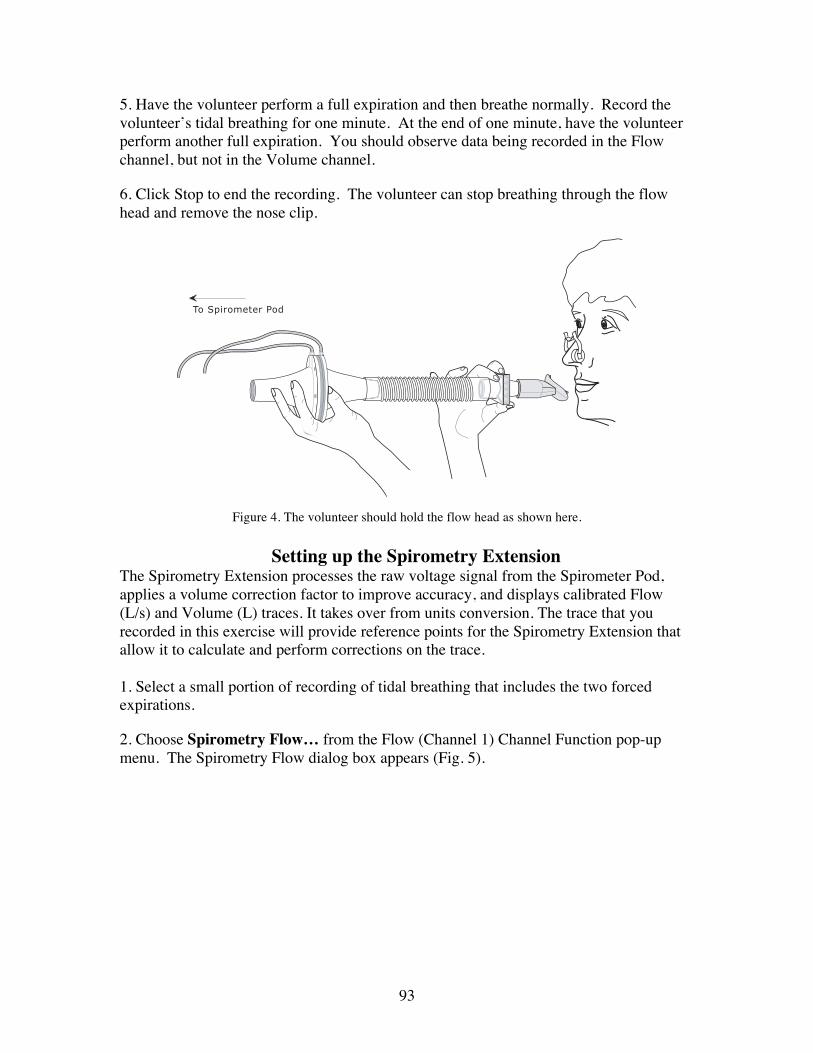
93
5. Have the volunteer perform a full expiration and then breathe normally. Record the volunteer’s tidal breathing for one minute. At the end of one minute, have the volunteer perform another full expiration. You should observe data being recorded in the Flow channel, but not in the Volume channel.
6. Click Stop to end the recording. The volunteer can stop breathing through the flow head and remove the nose clip.
Figure 4. The volunteer should hold the flow head as shown here.
Setting up the Spirometry Extension
The Spirometry Extension processes the raw voltage signal from the Spirometer Pod, applies a volume correction factor to improve accuracy, and displays calibrated Flow (L/s) and Volume (L) traces. It takes over from units conversion. The trace that you recorded in this exercise will provide reference points for the Spirometry Extension that allow it to calculate and perform corrections on the trace. 1. Select a small portion of recording of tidal breathing that includes the two forced expirations.
2. Choose Spirometry Flow… from the Flow (Channel 1) Channel Function pop-up menu. The Spirometry Flow dialog box appears (Fig. 5).
To Spirometer Pod
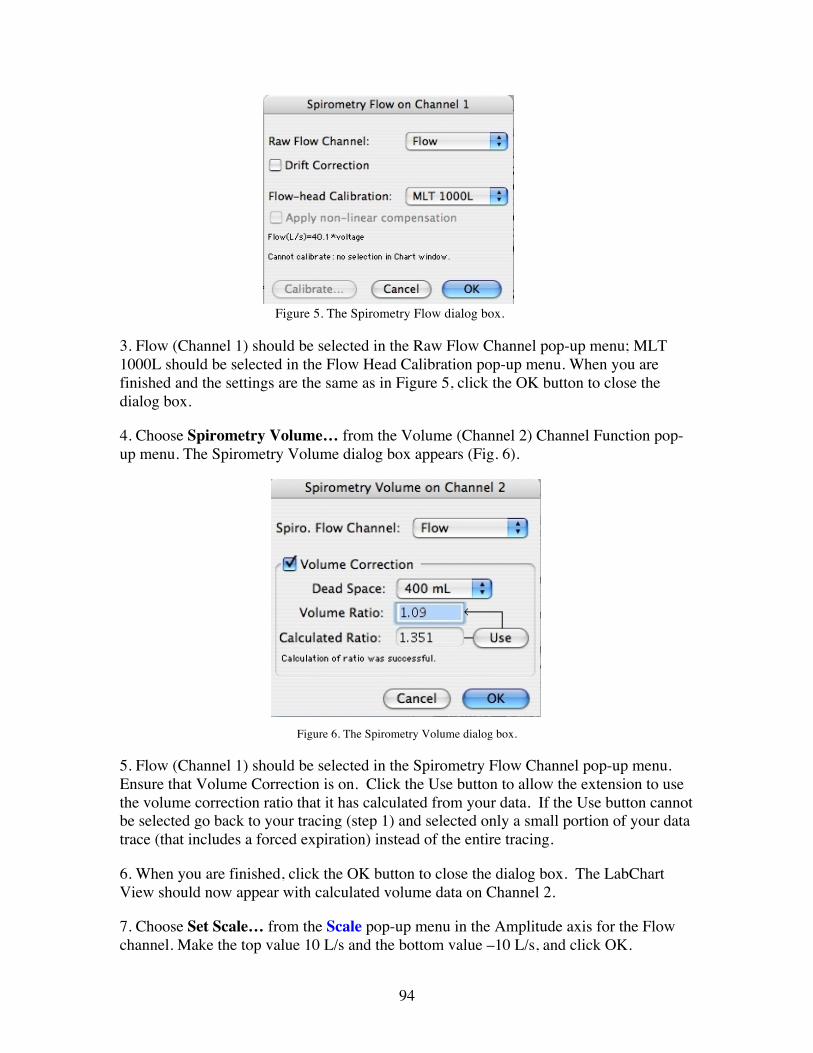
94
Figure 5. The Spirometry Flow dialog box.
3. Flow (Channel 1) should be selected in the Raw Flow Channel pop-up menu; MLT 1000L should be selected in the Flow Head Calibration pop-up menu. When you are finished and the settings are the same as in Figure 5, click the OK button to close the dialog box.
4. Choose Spirometry Volume… from the Volume (Channel 2) Channel Function pop-up menu. The Spirometry Volume dialog box appears (Fig. 6).
Figure 6. The Spirometry Volume dialog box.
5. Flow (Channel 1) should be selected in the Spirometry Flow Channel pop-up menu. Ensure that Volume Correction is on. Click the Use button to allow the extension to use the volume correction ratio that it has calculated from your data. If the Use button cannot be selected go back to your tracing (step 1) and selected only a small portion of your data trace (that includes a forced expiration) instead of the entire tracing.
6. When you are finished, click the OK button to close the dialog box. The LabChart View should now appear with calculated volume data on Channel 2.
7. Choose Set Scale… from the Scale pop-up menu in the Amplitude axis for the Flow channel. Make the top value 10 L/s and the bottom value –10 L/s, and click OK.
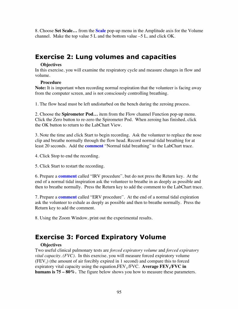
95
8. Choose Set Scale… from the Scale pop-up menu in the Amplitude axis for the Volume channel. Make the top value 5 L and the bottom value –5 L, and click OK.
Exercise 2: Lung volumes and capacities Objectives
In this exercise, you will examine the respiratory cycle and measure changes in flow and volume.
Procedure Note: It is important when recording normal respiration that the volunteer is facing away from the computer screen, and is not consciously controlling breathing. 1. The flow head must be left undisturbed on the bench during the zeroing process.
2. Choose the Spirometer Pod… item from the Flow channel Function pop-up menu. Click the Zero button to re-zero the Spirometer Pod. When zeroing has finished, click the OK button to return to the LabChart View.
3. Note the time and click Start to begin recording. Ask the volunteer to replace the nose clip and breathe normally through the flow head. Record normal tidal breathing for at least 20 seconds. Add the comment “Normal tidal breathing” to the LabChart trace.
4. Click Stop to end the recording.
5. Click Start to restart the recording.
6. Prepare a comment called “IRV procedure”, but do not press the Return key. At the end of a normal tidal inspiration ask the volunteer to breathe in as deeply as possible and then to breathe normally. Press the Return key to add the comment to the LabChart trace.
7. Prepare a comment called “ERV procedure”. At the end of a normal tidal expiration ask the volunteer to exhale as deeply as possible and then to breathe normally. Press the Return key to add the comment.
8. Using the Zoom Window, print out the experimental results.
Exercise 3: Forced Expiratory Volume
Objectives Two useful clinical pulmonary tests are forced expiratory volume and forced expiratory vital capacity. (FVC). In this exercise, you will measure forced expiratory volume (FEV1) (the amount of air forcibly expired in 1 second) and compare this to forced expiratory vital capacity using the equation,FEV1//FVC. Average FEV1/FVC in humans is 75 – 80%. The figure below shows you how to measure these parameters.
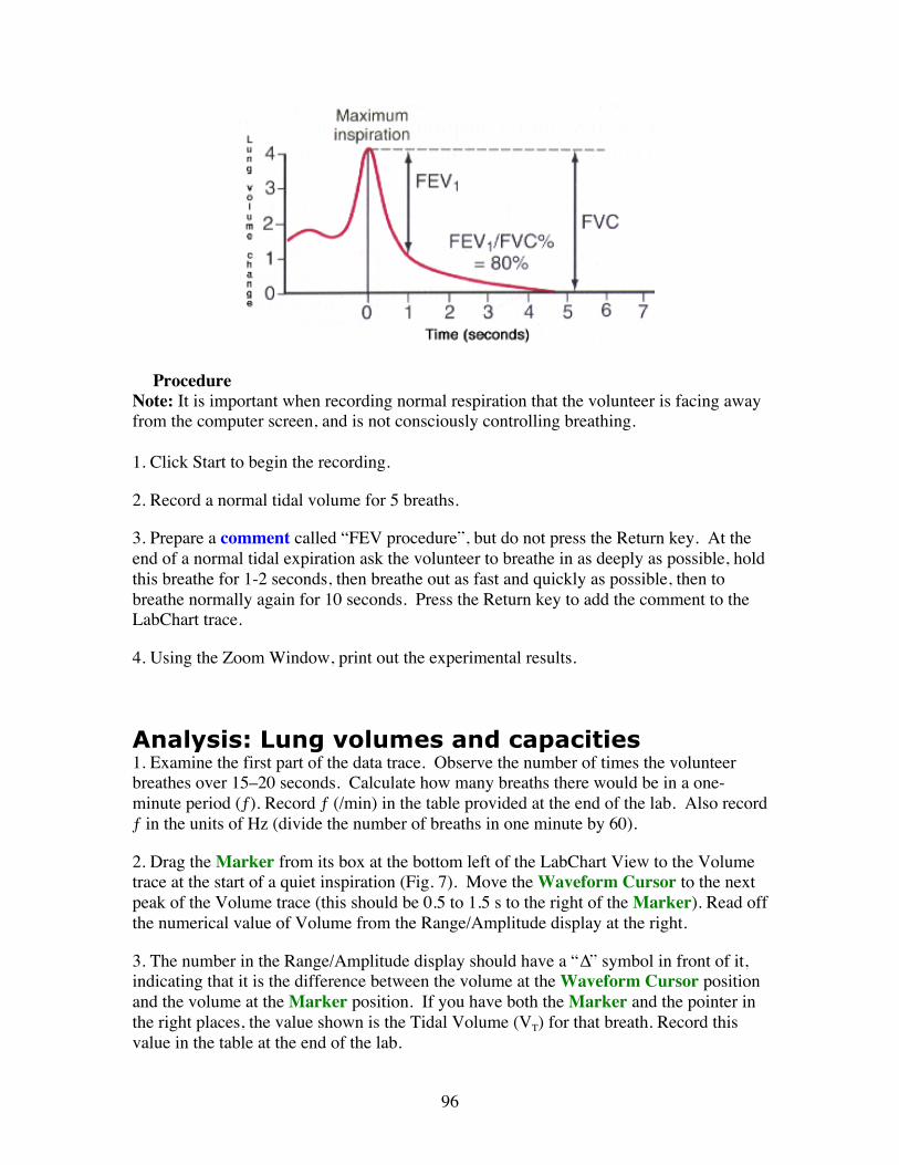
96
Procedure Note: It is important when recording normal respiration that the volunteer is facing away from the computer screen, and is not consciously controlling breathing. 1. Click Start to begin the recording.
2. Record a normal tidal volume for 5 breaths.
3. Prepare a comment called “FEV procedure”, but do not press the Return key. At the end of a normal tidal expiration ask the volunteer to breathe in as deeply as possible, hold this breathe for 1-2 seconds, then breathe out as fast and quickly as possible, then to breathe normally again for 10 seconds. Press the Return key to add the comment to the LabChart trace.
4. Using the Zoom Window, print out the experimental results.
Analysis: Lung volumes and capacities 1. Examine the first part of the data trace. Observe the number of times the volunteer breathes over 15–20 seconds. Calculate how many breaths there would be in a one-minute period (ƒ). Record ƒ (/min) in the table provided at the end of the lab. Also record ƒ in the units of Hz (divide the number of breaths in one minute by 60).
2. Drag the Marker from its box at the bottom left of the LabChart View to the Volume trace at the start of a quiet inspiration (Fig. 7). Move the Waveform Cursor to the next peak of the Volume trace (this should be 0.5 to 1.5 s to the right of the Marker). Read off the numerical value of Volume from the Range/Amplitude display at the right.
3. The number in the Range/Amplitude display should have a “∆” symbol in front of it, indicating that it is the difference between the volume at the Waveform Cursor position and the volume at the Marker position. If you have both the Marker and the pointer in the right places, the value shown is the Tidal Volume (VT) for that breath. Record this value in the table at the end of the lab.
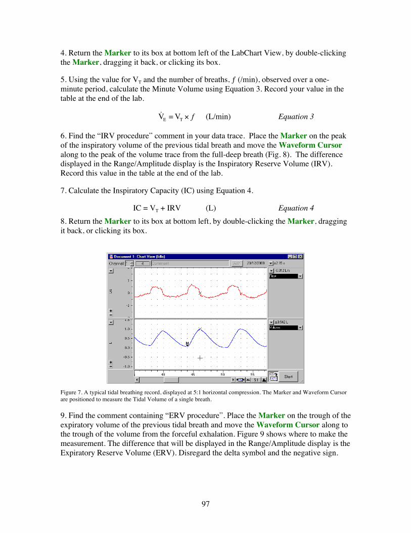
97
4. Return the Marker to its box at bottom left of the LabChart View, by double-clicking the Marker, dragging it back, or clicking its box.
5. Using the value for VT and the number of breaths, ƒ (/min), observed over a one-minute period, calculate the Minute Volume using Equation 3. Record your value in the table at the end of the lab.
!
˙ V E = VT " f (L/min) Equation 3 6. Find the “IRV procedure” comment in your data trace. Place the Marker on the peak of the inspiratory volume of the previous tidal breath and move the Waveform Cursor along to the peak of the volume trace from the full-deep breath (Fig. 8). The difference displayed in the Range/Amplitude display is the Inspiratory Reserve Volume (IRV). Record this value in the table at the end of the lab.
7. Calculate the Inspiratory Capacity (IC) using Equation 4.
IC = VT + IRV (L) Equation 4 8. Return the Marker to its box at bottom left, by double-clicking the Marker, dragging it back, or clicking its box.
Figure 7. A typical tidal breathing record, displayed at 5:1 horizontal compression. The Marker and Waveform Cursor are positioned to measure the Tidal Volume of a single breath.
9. Find the comment containing “ERV procedure”. Place the Marker on the trough of the expiratory volume of the previous tidal breath and move the Waveform Cursor along to the trough of the volume from the forceful exhalation. Figure 9 shows where to make the measurement. The difference that will be displayed in the Range/Amplitude display is the Expiratory Reserve Volume (ERV). Disregard the delta symbol and the negative sign.
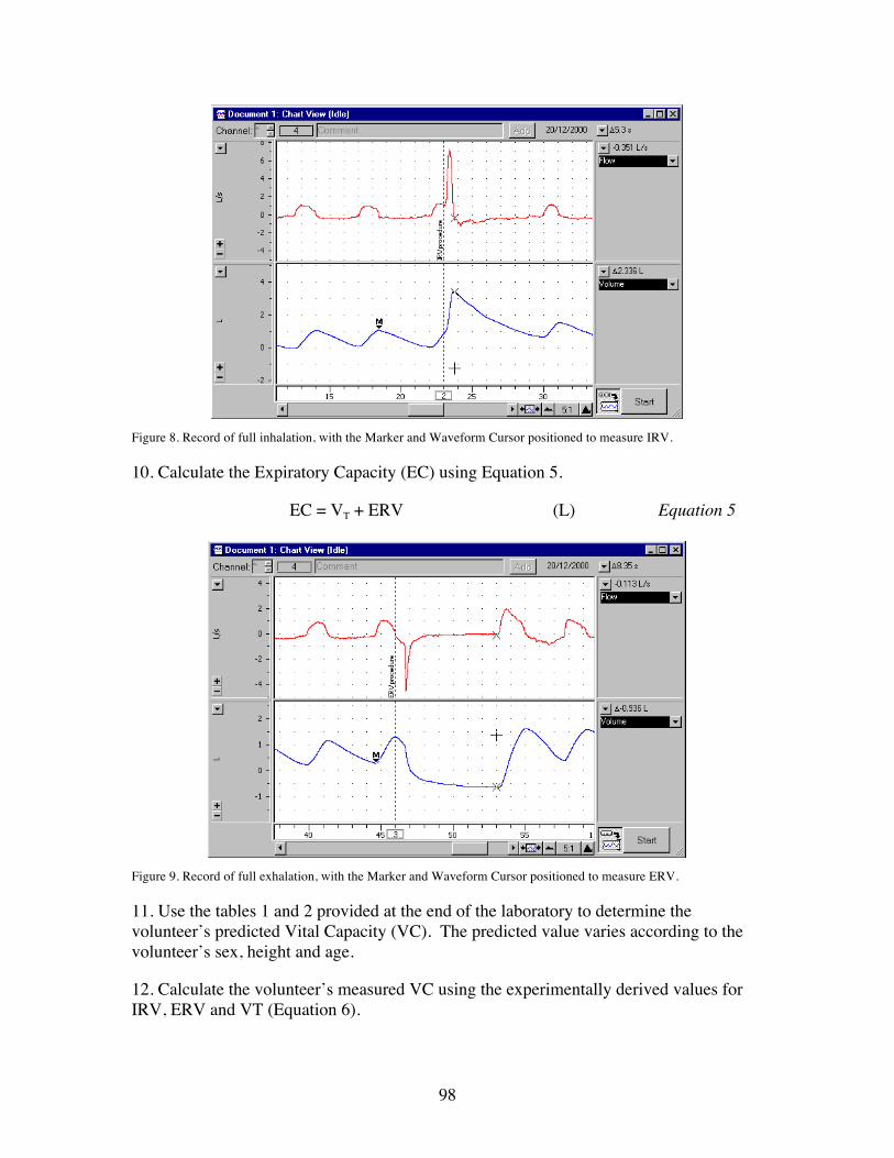
98
Figure 8. Record of full inhalation, with the Marker and Waveform Cursor positioned to measure IRV.
10. Calculate the Expiratory Capacity (EC) using Equation 5.
EC = VT + ERV (L) Equation 5
Figure 9. Record of full exhalation, with the Marker and Waveform Cursor positioned to measure ERV.
11. Use the tables 1 and 2 provided at the end of the laboratory to determine the volunteer’s predicted Vital Capacity (VC). The predicted value varies according to the volunteer’s sex, height and age.
12. Calculate the volunteer’s measured VC using the experimentally derived values for IRV, ERV and VT (Equation 6).
99
VC = IRV + ERV + VT (L) Equation 6
13. Residual Volume (RV) is the volume of gas remaining in the lungs after a maximal expiration. The RV cannot be determined by spirometric recording. Using Equation 7, determine the predicted RV value for the volunteer. This equation predicts RV for 16–34 year-old subjects of either sex.
RV = predicted VC X 0.25 (L) Equation 7
14. The Total Lung Capacity (TLC) is the sum of the vital capacity and residual volume. Calculate the predicted TLC for the volunteer (Equation 8) using the predicted values for VC and RV.
TLC = VC + RV (L) Equation 8
15. Functional Residual Capacity (FRC) is the volume of gas remaining in the lungs at the end of a normal tidal expiration (the sum of the RV and ERV). Calculate the FRC value for the volunteer using Equation 9.
FRC = ERV + RV (L) Equation 9
16. Forced Expiratory Volume (FEV1) is the volume of air expelled forcibly expelled from the lungs in 1 second. Find the “FEV” comment in your data trace. Place the Marker on the peak of the inspiratory volume and move the Waveform Cursor along the tracing until 1 second past the peak of the volume trace from the full-deep breath. You may need to increase the scales on the X- and Y-axes. Record the FEV1 value in the table. Calculate FEV1 using Equation 10.
!
FEV1 =volume of air expired in 1sec.
FVC (L) Equation 10
II. Measuring chest expansion In these experiments, you will record breathing movements with a respiratory belt transducer fastened around the abdomen. You will investigate various aspects of breathing (i.e., how breathing is effected under various conditions). Initially each group will conduct the standard “normal breathing” experiment. Thereafter you will be asked to design experiments to test changes in breathing under various conditions. PowerLab procedures – Measuring chest expansion A. Set up and calibration of equipment 1. The Respiratory Belt should be attached to BNC connector in Channel 2. Locate LabChart on your computer and start the software.
2. From the Experiments Gallery dialog box, select “Breathing” from the left-hand list. Select the settings file “Breath Settings” from the right-hand list, and
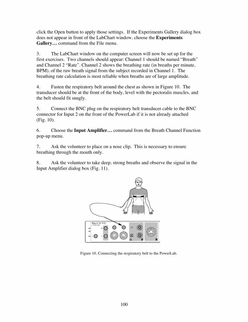
100
click the Open button to apply those settings. If the Experiments Gallery dialog box does not appear in front of the LabChart window, choose the Experiments Gallery… command from the File menu.
3. The LabChart window on the computer screen will now be set up for the first exercises. Two channels should appear: Channel 1 should be named “Breath” and Channel 2 “Rate”. Channel 2 shows the breathing rate (in breaths per minute, BPM), of the raw breath signal from the subject recorded in Channel 1. The breathing rate calculation is most reliable when breaths are of large amplitude.
4. Fasten the respiratory belt around the chest as shown in Figure 10. The transducer should be at the front of the body, level with the pectoralis muscles, and the belt should fit snugly.
5. Connect the BNC plug on the respiratory belt transducer cable to the BNC connector for Input 2 on the front of the PowerLab if it is not already attached (Fig. 10).
6. Choose the Input Amplifier… command from the Breath Channel Function pop-up menu.
7. Ask the volunteer to place on a nose clip. This is necessary to ensure breathing through the mouth only.
8. Ask the volunteer to take deep, strong breaths and observe the signal in the Input Amplifier dialog box (Fig. 11).
Figure 10. Connecting the respiratory belt to the PowerLab.
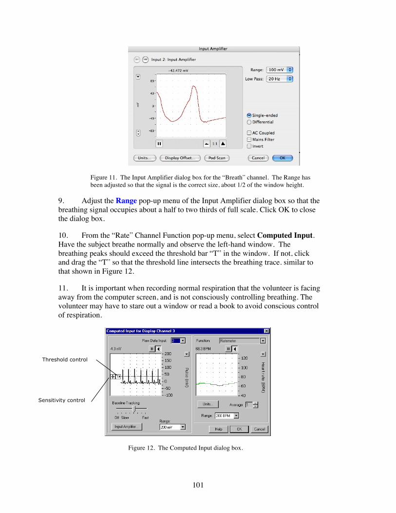
101
Figure 11. The Input Amplifier dialog box for the “Breath” channel. The Range has been adjusted so that the signal is the correct size, about 1/2 of the window height.
9. Adjust the Range pop-up menu of the Input Amplifier dialog box so that the breathing signal occupies about a half to two thirds of full scale. Click OK to close the dialog box.
10. From the “Rate” Channel Function pop-up menu, select Computed Input. Have the subject breathe normally and observe the left-hand window. The breathing peaks should exceed the threshold bar “T” in the window. If not, click and drag the “T” so that the threshold line intersects the breathing trace. similar to that shown in Figure 12.
11. It is important when recording normal respiration that the volunteer is facing away from the computer screen, and is not consciously controlling breathing. The volunteer may have to stare out a window or read a book to avoid conscious control of respiration.
Figure 12. The Computed Input dialog box.
Threshold control
Sensitivity control
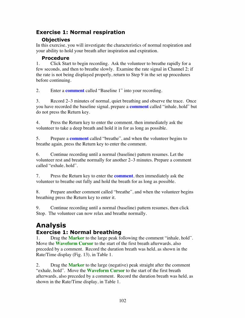
102
Exercise 1: Normal respiration Objectives
In this exercise, you will investigate the characteristics of normal respiration and your ability to hold your breath after inspiration and expiration.
Procedure 1. Click Start to begin recording. Ask the volunteer to breathe rapidly for a few seconds, and then to breathe slowly. Examine the rate signal in Channel 2; if the rate is not being displayed properly, return to Step 9 in the set up procedures before continuing.
2. Enter a comment called “Baseline 1” into your recording.
3. Record 2–3 minutes of normal, quiet breathing and observe the trace. Once you have recorded the baseline signal, prepare a comment called “inhale, hold” but do not press the Return key.
4. Press the Return key to enter the comment, then immediately ask the volunteer to take a deep breath and hold it in for as long as possible.
5. Prepare a comment called “breathe”, and when the volunteer begins to breathe again, press the Return key to enter the comment.
6. Continue recording until a normal (baseline) pattern resumes. Let the volunteer rest and breathe normally for another 2–3 minutes. Prepare a comment called “exhale, hold”.
7. Press the Return key to enter the comment, then immediately ask the volunteer to breathe out fully and hold the breath for as long as possible.
8. Prepare another comment called “breathe”, and when the volunteer begins breathing press the Return key to enter it.
9. Continue recording until a normal (baseline) pattern resumes, then click Stop. The volunteer can now relax and breathe normally.
Analysis Exercise 1: Normal breathing 1. Drag the Marker to the large peak following the comment “inhale, hold”. Move the Waveform Cursor to the start of the first breath afterwards, also preceded by a comment. Record the duration breath was held, as shown in the Rate/Time display (Fig. 13), in Table 1.
2. Drag the Marker to the large (negative) peak straight after the comment “exhale, hold”. Move the Waveform Cursor to the start of the first breath afterwards, also preceded by a comment. Record the duration breath was held, as shown in the Rate/Time display, in Table 1.
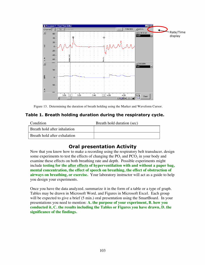
103
Figure 13. Determining the duration of breath holding using the Marker and Waveform Cursor.
Table 1. Breath holding duration during the respiratory cycle.
Condition Breath hold duration (sec) Breath hold after inhalation
Breath hold after exhalation
Oral presentation Activity Now that you know how to make a recording using the respiratory belt transducer, design some experiments to test the effects of changing the PO2 and PCO2 in your body and examine these effects on both breathing rate and depth. Possible experiments might include testing for the after effects of hyperventilation with and without a paper bag, mental concentration, the effect of speech on breathing, the effect of obstruction of airways on breathing, or exercise. Your laboratory instructor will act as a guide to help you design your experiments. Once you have the data analyzed, summarize it in the form of a table or a type of graph. Tables may be drawn in Microsoft Word, and Figures in Microsoft Excel. Each group will be expected to give a brief (5 min.) oral presentation using the SmartBoard. In your presentations you need to mention: A. the purpose of your experiment, B. how you conducted it, C. the results including the Tables or Figures you have drawn, D. the significance of the findings.
Rate/Time display
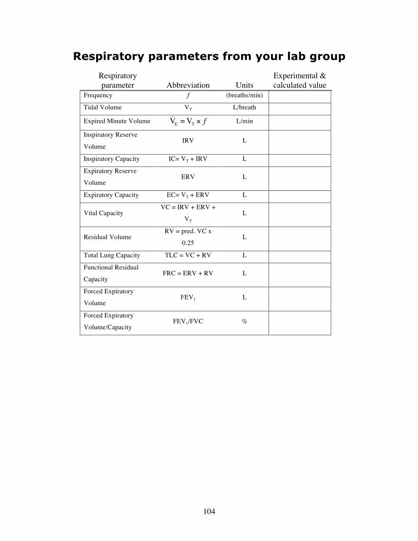
104
Respiratory parameters from your lab group
Respiratory parameter Abbreviation Units
Experimental & calculated value
Frequency f (breaths/min)
Tidal Volume VT L/breath
Expired Minute Volume
!
˙ V E = VT " f L/min
Inspiratory Reserve
Volume IRV L
Inspiratory Capacity IC= VT + IRV L
Expiratory Reserve
Volume ERV L
Expiratory Capacity EC= VT + ERV L
Vital Capacity VC = IRV + ERV +
VT L
Residual Volume RV = pred. VC x
0.25 L
Total Lung Capacity TLC = VC + RV L
Functional Residual
Capacity FRC = ERV + RV L
Forced Expiratory
Volume FEV1 L
Forced Expiratory
Volume/Capacity FEV1/FVC %
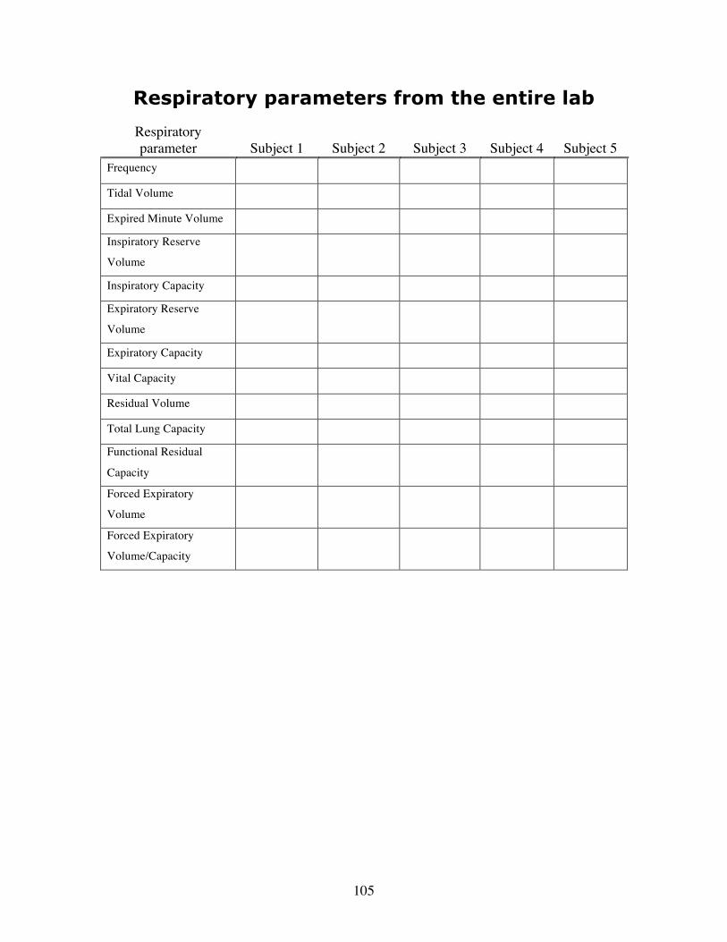
105
Respiratory parameters from the entire lab
Respiratory parameter Subject 1 Subject 2 Subject 3 Subject 4 Subject 5
Frequency
Tidal Volume
Expired Minute Volume Inspiratory Reserve
Volume
Inspiratory Capacity Expiratory Reserve
Volume
Expiratory Capacity
Vital Capacity
Residual Volume
Total Lung Capacity Functional Residual
Capacity
Forced Expiratory
Volume
Forced Expiratory
Volume/Capacity
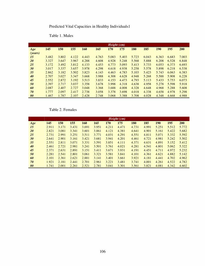
106
Predicted Vital Capacities in Healthy Individuals1
Table 1. Males
Height (cm) Age (years)
145 150 155 160 165 170 175 180 185 190 195 200
15 3.482 3.802 4.122 4.443 4.763 5.083 5.403 5.723 6.043 6.363 6.683 7.003 20 3.327 3.647 3.967 4.288 4.608 4.928 5.248 5.568 5.888 6.208 6.528 6.848 25 3.172 3.492 3.812 4.133 4.453 4.773 5.093 5.413 5.733 6.053 6.373 6.693 30 3.017 3.337 3.657 3.978 4.298 4.618 4.938 5.258 5.578 5.898 6.218 6.538 35 2.862 3.182 3.502 3.823 4.143 4.463 4.783 5.103 5.423 5.743 6.063 6.383 40 2.707 3.027 3.347 3.668 3.988 4.308 4.628 4.948 5.268 5.588 5.908 6.228 45 2.552 2.872 3.192 3.513 3.833 4.153 4.473 4.793 5.113 5.433 5.753 6.073 50 2.397 2.717 3.037 3.358 3.678 3.998 4.318 4.638 4.958 5.278 5.598 5.918 60 2.087 2.407 2.727 3.048 3.368 3.688 4.008 4.328 4.648 4.968 5.288 5.608 70 1.777 2.097 2.417 2.738 3.058 3.378 3.698 4.018 4.338 4.658 4.978 5.298 80 1.467 1.787 2.107 2.428 2.748 3.068 3.388 3.708 4.028 4.348 4.668 4.988
Table 2. Females
Height (cm) Age 145 150 155 160 165 170 175 180 185 190 195 200 15 2.911 3.171 3.431 3.691 3.951 4.211 4.471 4.731 4.991 5.251 5.512 5.772 20 2.821 3.081 3.341 3.601 3.861 4.121 4.381 4.641 4.901 5.161 5.422 5.682 25 2.731 2.991 3.251 3.511 3.771 4.031 4.291 4.551 4.811 5.071 5.332 5.592 30 2.641 2.901 3.161 3.421 3.681 3.941 4.201 4.461 4.721 4.981 5.242 5.502 35 2.551 2.811 3.071 3.331 3.591 3.851 4.111 4.371 4.631 4.891 5.152 5.412 40 2.461 2.721 2.981 3.241 3.501 3.761 4.021 4.281 4.541 4.801 5.062 5.322 45 2.371 2.631 2.891 3.151 3.411 3.671 3.931 4.191 4.451 4.711 4.972 5.232 50 2.281 2.541 2.801 3.061 3.321 3.581 3.841 4.101 4.361 4.621 4.882 5.142 60 2.101 2.361 2.621 2.881 3.141 3.401 3.661 3.921 4.181 4.441 4.702 4.962 70 1.921 2.181 2.441 2.701 2.961 3.221 3.481 3.741 4.001 4.261 4.522 4.782 80 1.741 2.001 2.261 2.521 2.781 3.041 3.301 3.561 3.821 4.081 4.342 4.602
107
Study Questions 1. Compare your experimental findings with your predicted results. Do any of the parameters differ significantly? If so, what factors influenced the results?
2. Describe normal respiratory movements. What is the physiological mechanism responsible for inspiration? What is the physiological mechanism responsible for expiration?
3. Hyperventilation results in hypocapnia, while re-breathing from a closed bag results in hypercapnia. How do these conditions affect respiratory rate and depth?
108
Osmoregulation Introduction The vertebrate kidney has many different functions. One of the most important functions is to regulate the osmolality of body fluids. This is particularly important considering that a body cell’s membrane has the ability to flux water up to 100 times the cell volume every second. Thus maintaining a constant concentration of solutes in the extracellular fluid is imperative if the cell is to maintain its normal functions. In mammals, plasma osmolality averages 290 mOsm with a small range of only ± 5 mOsm. Plasma osmolality in non-mammalian vertebrates fluctuates more than just ± 5 mOsm. Fish and amphibians are particularly susceptible to changes in plasma osmolality due to their relatively porous integument. Plasma osmolality in reptiles and birds is slightly more stable but varies more than is seen in mammals. For example, typical plasma osmolalities in birds is 320 mOsm (± 50). The vertebrate kidney regulates the overall concentration of plasma osmolality by regulating the amount of substances excreted in the urine. For example, the concentration of hydrogen ions is maintained by the kidneys, and normally ranges from 4.5 – 8 in mammals. Substances such as proteins circulate in the blood. Proteins are filtered into the kidneys in uricotelic vertebrates such as reptiles and birds, but not in ureotelic vertebrates such as amphibians and mammals. Hence, the presence of protein in the urine of ureotelic vertebrates (i.e., proteinuria) is a classic sign of damage to the filtration membrane of the glomerulus in the kidney. Red blood cells are not normally filtered in any class of vertebrate, and the presence of blood in the urine is also indicative of damage to the glomerular filtration membrane. Vertebrates also handle glucose very differently. Some animals like birds are naturally diabetic. Hummingbirds (that feed on almost a purely nectarivorous diet) for example, excreting as much as 600mg/ml glucose in their urine. High glucose levels in humans (glucosuria) however, may be a sign of diabetes mellitus, a condition caused by an abnormally low production of insulin by the pancreas. The following experiment will test the kidney’s ability to regulate plasma osmolality when faced with ingestion of hyperosmotic, isotonic and hypotonic solutions. Objectives • To test the mammalian kidney’s ability to regulate urine volume and concentration when faced with conditions of dehydration, normal hydration and over hydration. • To test to mammalian kidney’s ability to control variables such as pH, protein, glucose and blood in the urine. • To test the kidney’s ability to produce a concentrated urine by measuring specific gravity and osmolality.
109
Required equipment Urine collection containers Drinking containers (1L) Urinating containers of varying sizes Urinometer cylinders Celsius thermometers Hand-held refractometer 5 ml disposable test tubes (20/table) Graduated cylinders (100, 200 and 500 ml volumes) Pasteur pipettes and bulbs
20% potassium chromate 2.9% silver nitrate Labstix tests Gatorade No Fear energy drink Distilled water Kim wipes Osmometer and supplies
Experimental procedure 1. Before the experiment: Make certain you keep hydrated the day of the experiment (i.e., before coming into lab). Drink only water (no caffeine or soda). Eat only a light lunch consisting of a plain sandwich with little to no condiments. Empty your bladder 1 to 2 hours before the laboratory begins and record the exact time. Do not save this urine sample. 2. After the prelab, take a urine container to the restroom and void your bladder completely. Record the exact time. This sample will constitute the “control” urine sample. *CAUTION: if you suffer from high blood pressure or any other illness that may effect your blood pressure, please let your laboratory instructor know immediately before ingesting any of the solutions. 3. Upon returning to the lab, drink the designated solution as quickly as possible. The class will be divided up into three groups: Hyposmotic: drink 1,000 ml water
Isosmotic: drink 500 ml of Gatorade
Hyperosmotic: drink 200 ml of a high energy drink (Amp)
4. Every 30 minutes after drinking the solution above you need to perform the following tests. If you cannot void urine after a 30 minute period, record “zero” for the amount of urine produced, and retain urine in your bladder until the next 30 minute time interval. Tests to be perform every 30 minutes: a. Measure the volume of urine produced using the graduated cylinders provided in lab. Express the value in milliliters per minute in Table 1 in the Laboratory Report. b. Measure the specific gravity of the urine produced. Measurement of urine specific gravity is important in determining the ability of the kidney to concentrate or to dilute the urine. The inability of the kidneys to perform this function may be indicative of renal structural damage, metabolic disorders of endocrine disturbance.
110
The specific gravity of a liquid is defined as the ratio of the density of the substance being measured compared to the density of water at a specific temperature. The specific gravity of distilled water is 1.000. Measure the specific gravity of the urine by placing 1-2 drops of simulated urine on the prism of the urinometer then take a reading by looking through the ocular. Once finished clean the prism with a little water and wipe it dry with a kimwipe tissue. The normal range of urine specific gravity in humans is 1.001 to 1.035. Low values indicate a dilute urine and high values a concentrated urine. Measure the specific gravity of the urine by carefully pour urine from the urine container into the Urinometer cylinder (with the float inside it) and fill the Urinometer until the “float” begins to float. Record your results in the table in the Laboratory Report. If you produce less than about 150 ml of urine then use the hand-held refractometer to measure specific gravity. Your laboratory instructor will show you how to use the instrument. Caution: use only Kimwipe tissues to dry the prism. c. Measure the chloride concentration of the urine by placing 10 drops of urine into a 5 ml test tube using a Pasteur pipette. Add 1 drop of 20% potassium chromate. Add 2.9% silver nitrate solution drop by drop, shaking the mixture continuously while adding the drops (count the number of drops), until the mixture changes color from a bright yellow to a brown color. Each drop of 2.9% silver nitrate is equivalent to 61 mg of Cl- per 100 ml of urine. Therefore to obtain a chloride concentration in mg/100 ml, simply multiply the number of drops by 61. For example if 10 drops of 2.9% silver nitrate were required, 10 x 61 mg of Cl-/100 ml = 610 mg Cl-/100ml. Record the amount of NaCl in the urine in mg/dL in the table of the Laboratory Report. Test to be perform at the control and 60 minute time period: d. Measure urine osmolality by providing your instructor with one drop of your urine sample and he (she) will measure the osmolality. Place the data in the Table 3 in the Laboratory Report. Tests to be only once at 60 minute time period: Before performing these tests read the back of the Labstix bottle so that you are familiar with how the test operates. Measure the following parameters (glucose, blood, protein, pH and specific gravity) using the Labstix provided in the laboratory. Carefully take a stick out of the bottle (being careful not to place your fingers on the test strips), and immerse the stick in a beaker of urine. Gently lift the stick out of the beaker and remove any excess urine. After only a few seconds (instructions are on the back of the bottle of Labstix) begin to read the color LabChart. Place your individual results in table 2 in the Laboratory Report.
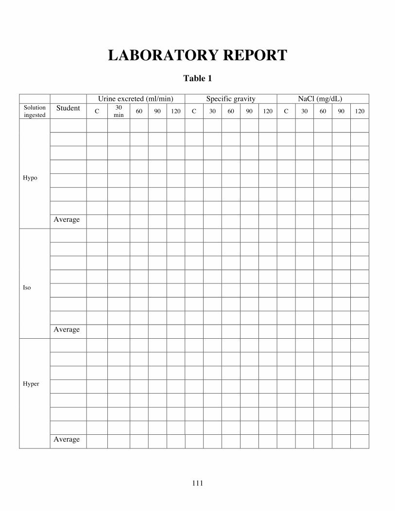
111
LABORATORY REPORT
Table 1
Urine excreted (ml/min) Specific gravity NaCl (mg/dL) Solution ingested
Student C 30 min 60 90 120 C 30 60 90 120 C 30 60 90 120
Hypo
Average
Iso
Average
Hyper
Average
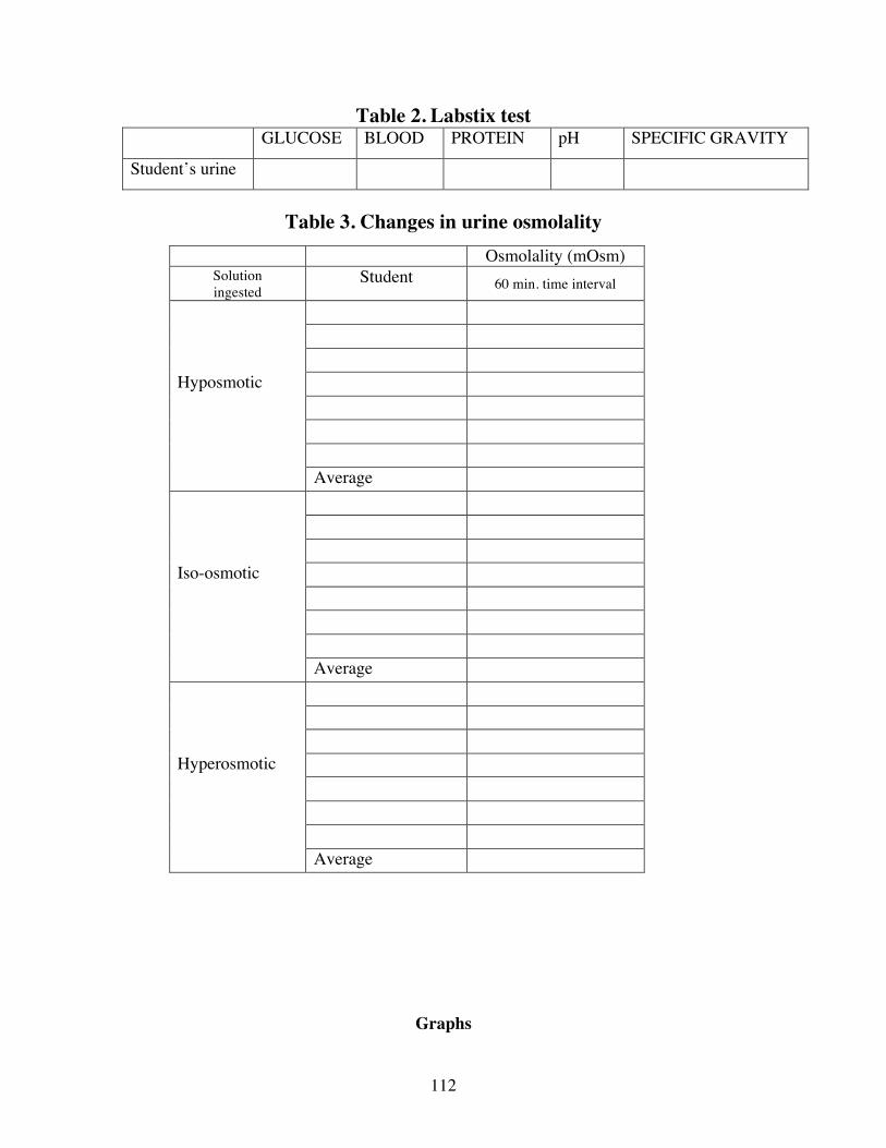
112
Table 2. Labstix test GLUCOSE BLOOD PROTEIN pH SPECIFIC GRAVITY
Student’s urine
Table 3. Changes in urine osmolality
Osmolality (mOsm) Solution ingested
Student 60 min. time interval
Hyposmotic Average Iso-osmotic Average Hyperosmotic Average
Graphs
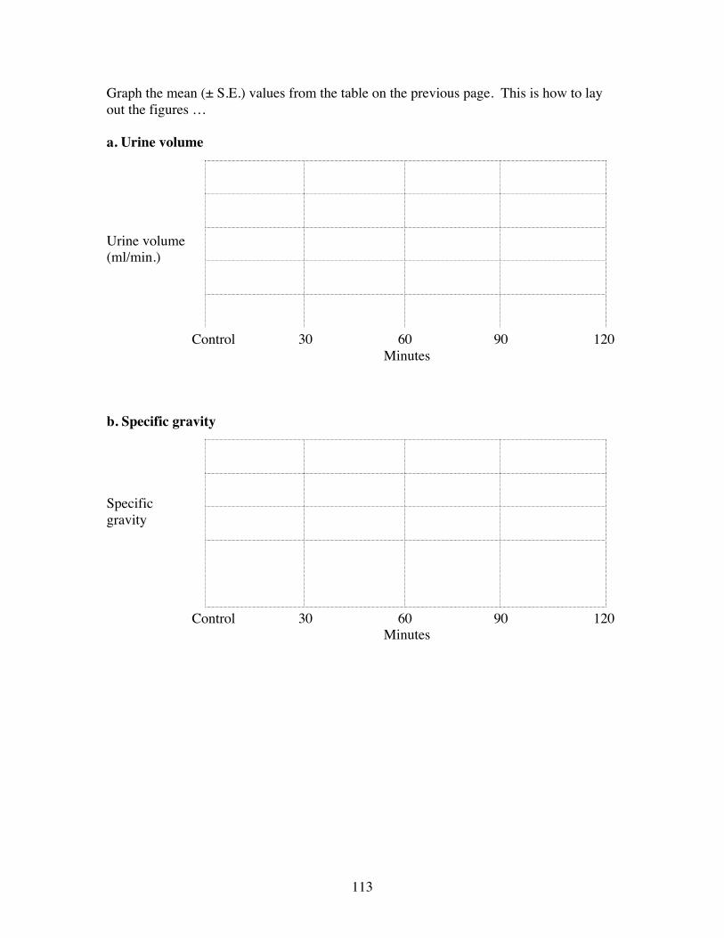
113
Graph the mean (± S.E.) values from the table on the previous page. This is how to lay out the figures … a. Urine volume Urine volume (ml/min.) Control 30 60 90 120 Minutes b. Specific gravity Specific gravity Control 30 60 90 120 Minutes
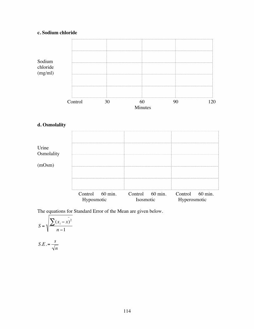
114
c. Sodium chloride Sodium chloride (mg/ml) Control 30 60 90 120 Minutes d. Osmolality Urine Osmolality (mOsm)
Control 60 min. Control 60 min. Control 60 min. Hyposmotic Isosmotic Hyperosmotic
The equations for Standard Error of the Mean are given below.
!
S =(xi " x)
2"
#n "1
!
S.E .= sn
115
Study questions Explain the physiological reasoning behind the data generated by each of your graphs with respect to each of the variables measured below. a. Urine volume
b. Specific gravity
c. Sodium Chloride

116
d. Osmolality
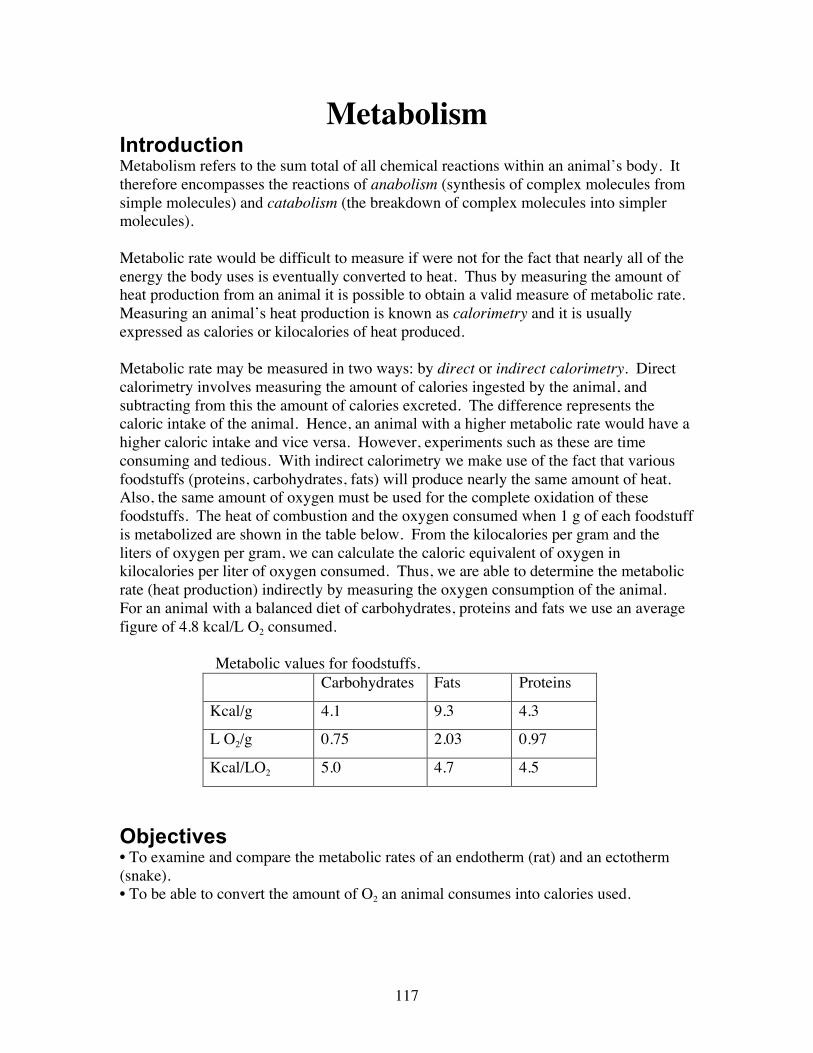
117
Metabolism Introduction Metabolism refers to the sum total of all chemical reactions within an animal’s body. It therefore encompasses the reactions of anabolism (synthesis of complex molecules from simple molecules) and catabolism (the breakdown of complex molecules into simpler molecules). Metabolic rate would be difficult to measure if were not for the fact that nearly all of the energy the body uses is eventually converted to heat. Thus by measuring the amount of heat production from an animal it is possible to obtain a valid measure of metabolic rate. Measuring an animal’s heat production is known as calorimetry and it is usually expressed as calories or kilocalories of heat produced. Metabolic rate may be measured in two ways: by direct or indirect calorimetry. Direct calorimetry involves measuring the amount of calories ingested by the animal, and subtracting from this the amount of calories excreted. The difference represents the caloric intake of the animal. Hence, an animal with a higher metabolic rate would have a higher caloric intake and vice versa. However, experiments such as these are time consuming and tedious. With indirect calorimetry we make use of the fact that various foodstuffs (proteins, carbohydrates, fats) will produce nearly the same amount of heat. Also, the same amount of oxygen must be used for the complete oxidation of these foodstuffs. The heat of combustion and the oxygen consumed when 1 g of each foodstuff is metabolized are shown in the table below. From the kilocalories per gram and the liters of oxygen per gram, we can calculate the caloric equivalent of oxygen in kilocalories per liter of oxygen consumed. Thus, we are able to determine the metabolic rate (heat production) indirectly by measuring the oxygen consumption of the animal. For an animal with a balanced diet of carbohydrates, proteins and fats we use an average figure of 4.8 kcal/L O2 consumed.
Metabolic values for foodstuffs. Carbohydrates Fats Proteins
Kcal/g 4.1 9.3 4.3
L O2/g 0.75 2.03 0.97
Kcal/LO2 5.0 4.7 4.5
Objectives • To examine and compare the metabolic rates of an endotherm (rat) and an ectotherm (snake). • To be able to convert the amount of O2 an animal consumes into calories used.
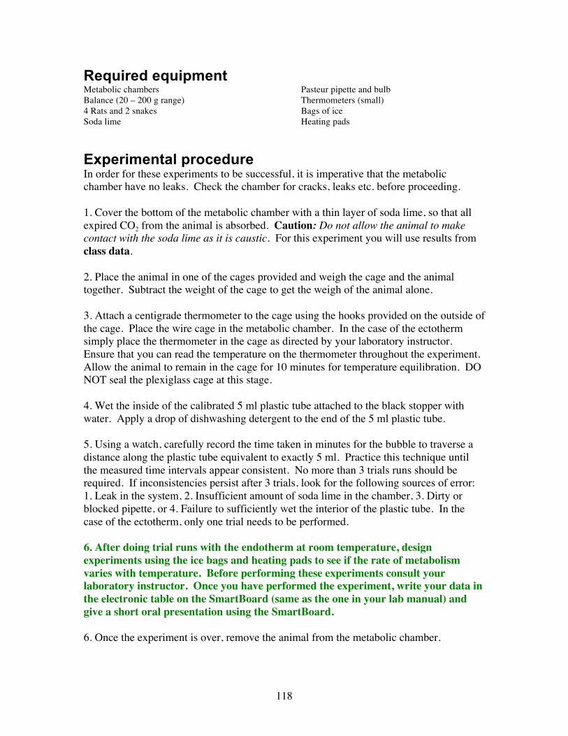
118
Required equipmentMetabolic chambers Balance (20 – 200 g range) 4 Rats and 2 snakes Soda lime
Pasteur pipette and bulb Thermometers (small) Bags of ice Heating pads
Experimental procedure In order for these experiments to be successful, it is imperative that the metabolic chamber have no leaks. Check the chamber for cracks, leaks etc. before proceeding. 1. Cover the bottom of the metabolic chamber with a thin layer of soda lime, so that all expired CO2 from the animal is absorbed. Caution: Do not allow the animal to make contact with the soda lime as it is caustic. For this experiment you will use results from class data. 2. Place the animal in one of the cages provided and weigh the cage and the animal together. Subtract the weight of the cage to get the weigh of the animal alone. 3. Attach a centigrade thermometer to the cage using the hooks provided on the outside of the cage. Place the wire cage in the metabolic chamber. In the case of the ectotherm simply place the thermometer in the cage as directed by your laboratory instructor. Ensure that you can read the temperature on the thermometer throughout the experiment. Allow the animal to remain in the cage for 10 minutes for temperature equilibration. DO NOT seal the plexiglass cage at this stage. 4. Wet the inside of the calibrated 5 ml plastic tube attached to the black stopper with water. Apply a drop of dishwashing detergent to the end of the 5 ml plastic tube. 5. Using a watch, carefully record the time taken in minutes for the bubble to traverse a distance along the plastic tube equivalent to exactly 5 ml. Practice this technique until the measured time intervals appear consistent. No more than 3 trials runs should be required. If inconsistencies persist after 3 trials, look for the following sources of error: 1. Leak in the system, 2. Insufficient amount of soda lime in the chamber, 3. Dirty or blocked pipette, or 4. Failure to sufficiently wet the interior of the plastic tube. In the case of the ectotherm, only one trial needs to be performed. 6. After doing trial runs with the endotherm at room temperature, design experiments using the ice bags and heating pads to see if the rate of metabolism varies with temperature. Before performing these experiments consult your laboratory instructor. Once you have performed the experiment, write your data in the electronic table on the SmartBoard (same as the one in your lab manual) and give a short oral presentation using the SmartBoard. 6. Once the experiment is over, remove the animal from the metabolic chamber.
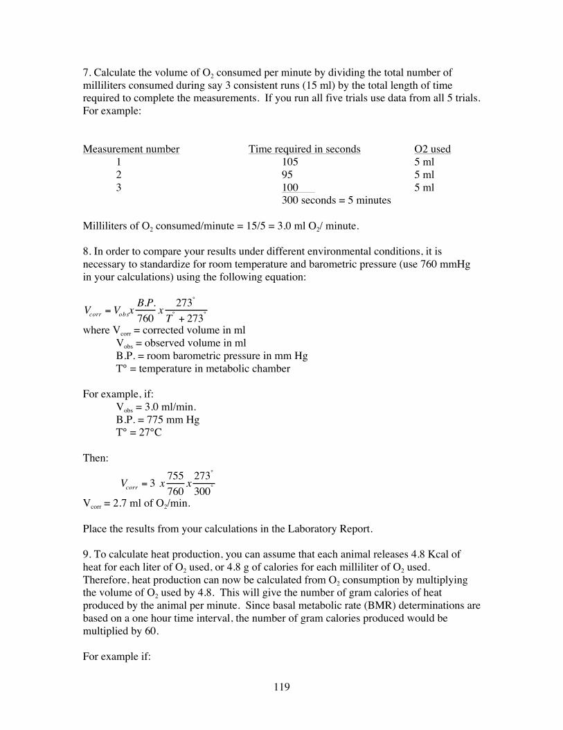
119
7. Calculate the volume of O2 consumed per minute by dividing the total number of milliliters consumed during say 3 consistent runs (15 ml) by the total length of time required to complete the measurements. If you run all five trials use data from all 5 trials. For example: Measurement number Time required in seconds O2 used 1 105 5 ml 2 95 5 ml 3 100 5 ml 300 seconds = 5 minutes Milliliters of O2 consumed/minute = 15/5 = 3.0 ml O2/ minute. 8. In order to compare your results under different environmental conditions, it is necessary to standardize for room temperature and barometric pressure (use 760 mmHg in your calculations) using the following equation:
where Vcorr = corrected volume in ml Vobs = observed volume in ml B.P. = room barometric pressure in mm Hg T° = temperature in metabolic chamber For example, if: Vobs = 3.0 ml/min. B.P. = 775 mm Hg T° = 27°C Then:
Vcorr = 2.7 ml of O2/min. Place the results from your calculations in the Laboratory Report. 9. To calculate heat production, you can assume that each animal releases 4.8 Kcal of heat for each liter of O2 used, or 4.8 g of calories for each milliliter of O2 used. Therefore, heat production can now be calculated from O2 consumption by multiplying the volume of O2 used by 4.8. This will give the number of gram calories of heat produced by the animal per minute. Since basal metabolic rate (BMR) determinations are based on a one hour time interval, the number of gram calories produced would be multiplied by 60. For example if:
Vcorr = VobsxB.P.760
x273°
T° + 273°
Vcorr = 3 x755760
x273°
300°
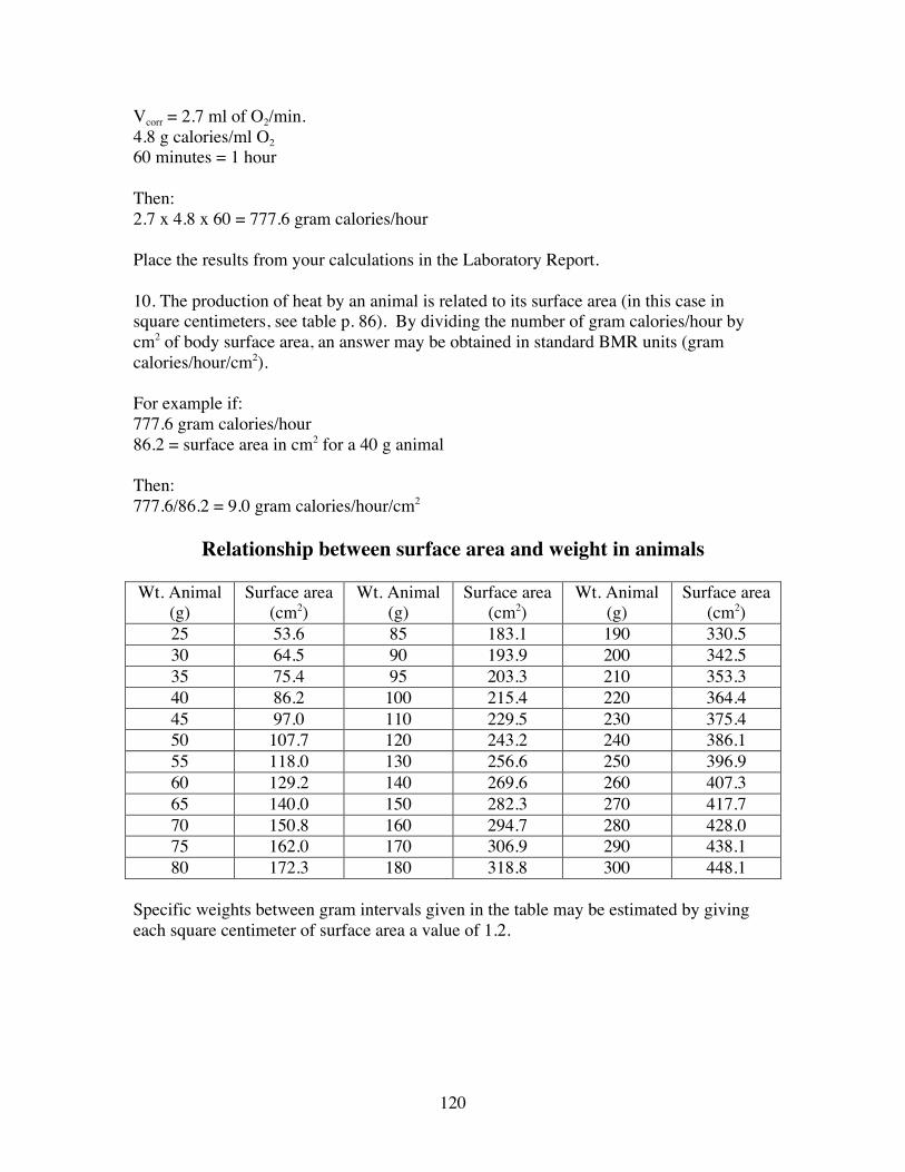
120
Vcorr = 2.7 ml of O2/min. 4.8 g calories/ml O2 60 minutes = 1 hour Then: 2.7 x 4.8 x 60 = 777.6 gram calories/hour Place the results from your calculations in the Laboratory Report. 10. The production of heat by an animal is related to its surface area (in this case in square centimeters, see table p. 86). By dividing the number of gram calories/hour by cm2 of body surface area, an answer may be obtained in standard BMR units (gram calories/hour/cm2). For example if: 777.6 gram calories/hour 86.2 = surface area in cm2 for a 40 g animal Then: 777.6/86.2 = 9.0 gram calories/hour/cm2
Relationship between surface area and weight in animals
Wt. Animal
(g) Surface area
(cm2) Wt. Animal
(g) Surface area
(cm2) Wt. Animal
(g) Surface area
(cm2) 25 53.6 85 183.1 190 330.5 30 64.5 90 193.9 200 342.5 35 75.4 95 203.3 210 353.3 40 86.2 100 215.4 220 364.4 45 97.0 110 229.5 230 375.4 50 107.7 120 243.2 240 386.1 55 118.0 130 256.6 250 396.9 60 129.2 140 269.6 260 407.3 65 140.0 150 282.3 270 417.7 70 150.8 160 294.7 280 428.0 75 162.0 170 306.9 290 438.1 80 172.3 180 318.8 300 448.1
Specific weights between gram intervals given in the table may be estimated by giving each square centimeter of surface area a value of 1.2.
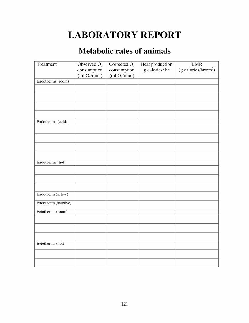
121
LABORATORY REPORT
Metabolic rates of animals
Treatment Observed O2 consumption (ml O2/min.)
Corrected O2 consumption (ml O2/min.)
Heat production g calories/ hr
BMR (g calories/hr/cm2)
Endotherms (room)
Endotherms (cold)
Endotherms (hot)
Endotherm (active) Endotherm (inactive) Ectotherms (room)
Ectotherms (hot)

122
Questions Why is metabolism expressed in units of surface area?
List 5 factors affecting metabolic rate and explain how each operates.

123
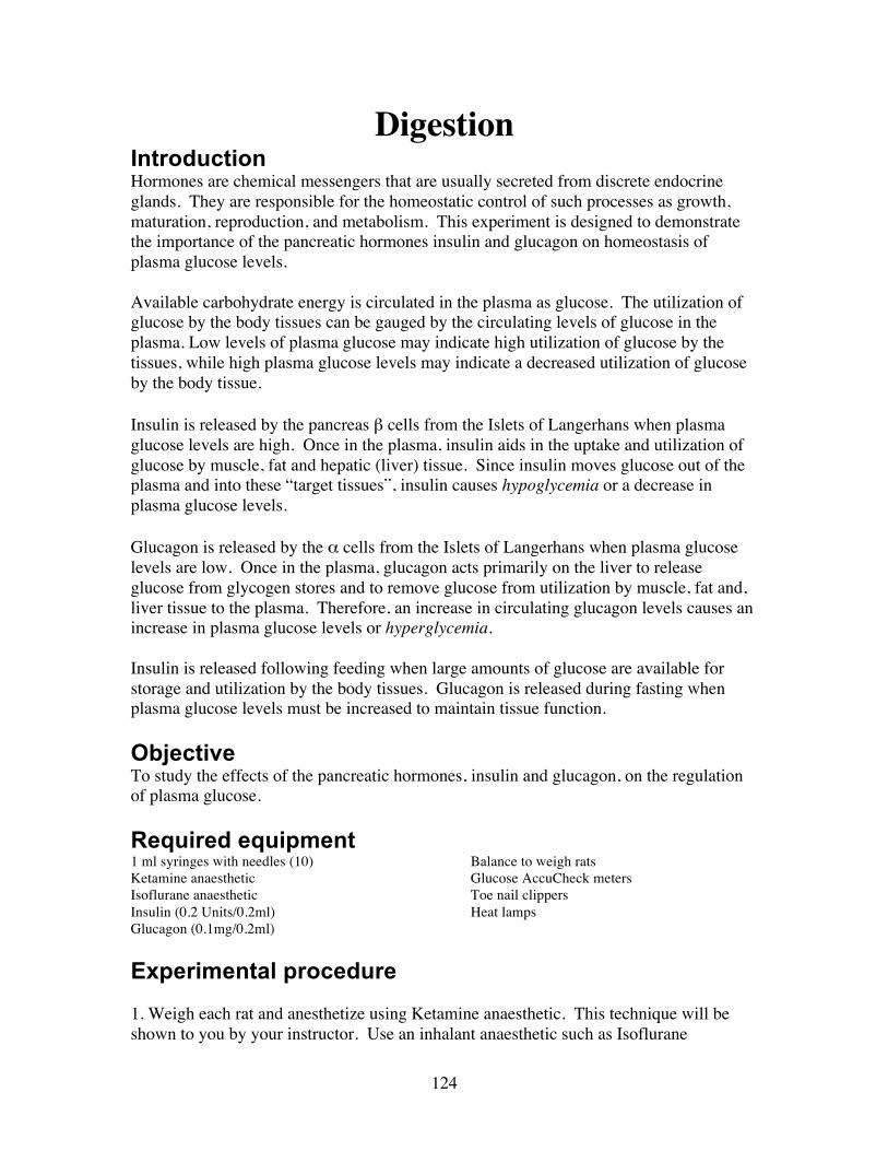
124
Digestion Introduction Hormones are chemical messengers that are usually secreted from discrete endocrine glands. They are responsible for the homeostatic control of such processes as growth, maturation, reproduction, and metabolism. This experiment is designed to demonstrate the importance of the pancreatic hormones insulin and glucagon on homeostasis of plasma glucose levels. Available carbohydrate energy is circulated in the plasma as glucose. The utilization of glucose by the body tissues can be gauged by the circulating levels of glucose in the plasma. Low levels of plasma glucose may indicate high utilization of glucose by the tissues, while high plasma glucose levels may indicate a decreased utilization of glucose by the body tissue. Insulin is released by the pancreas β cells from the Islets of Langerhans when plasma glucose levels are high. Once in the plasma, insulin aids in the uptake and utilization of glucose by muscle, fat and hepatic (liver) tissue. Since insulin moves glucose out of the plasma and into these “target tissues”, insulin causes hypoglycemia or a decrease in plasma glucose levels. Glucagon is released by the α cells from the Islets of Langerhans when plasma glucose levels are low. Once in the plasma, glucagon acts primarily on the liver to release glucose from glycogen stores and to remove glucose from utilization by muscle, fat and, liver tissue to the plasma. Therefore, an increase in circulating glucagon levels causes an increase in plasma glucose levels or hyperglycemia. Insulin is released following feeding when large amounts of glucose are available for storage and utilization by the body tissues. Glucagon is released during fasting when plasma glucose levels must be increased to maintain tissue function. Objective To study the effects of the pancreatic hormones, insulin and glucagon, on the regulation of plasma glucose. Required equipment1 ml syringes with needles (10) Ketamine anaesthetic Isoflurane anaesthetic Insulin (0.2 Units/0.2ml) Glucagon (0.1mg/0.2ml)
Balance to weigh rats Glucose AccuCheck meters Toe nail clippers Heat lamps
Experimental procedure 1. Weigh each rat and anesthetize using Ketamine anaesthetic. This technique will be shown to you by your instructor. Use an inhalant anaesthetic such as Isoflurane
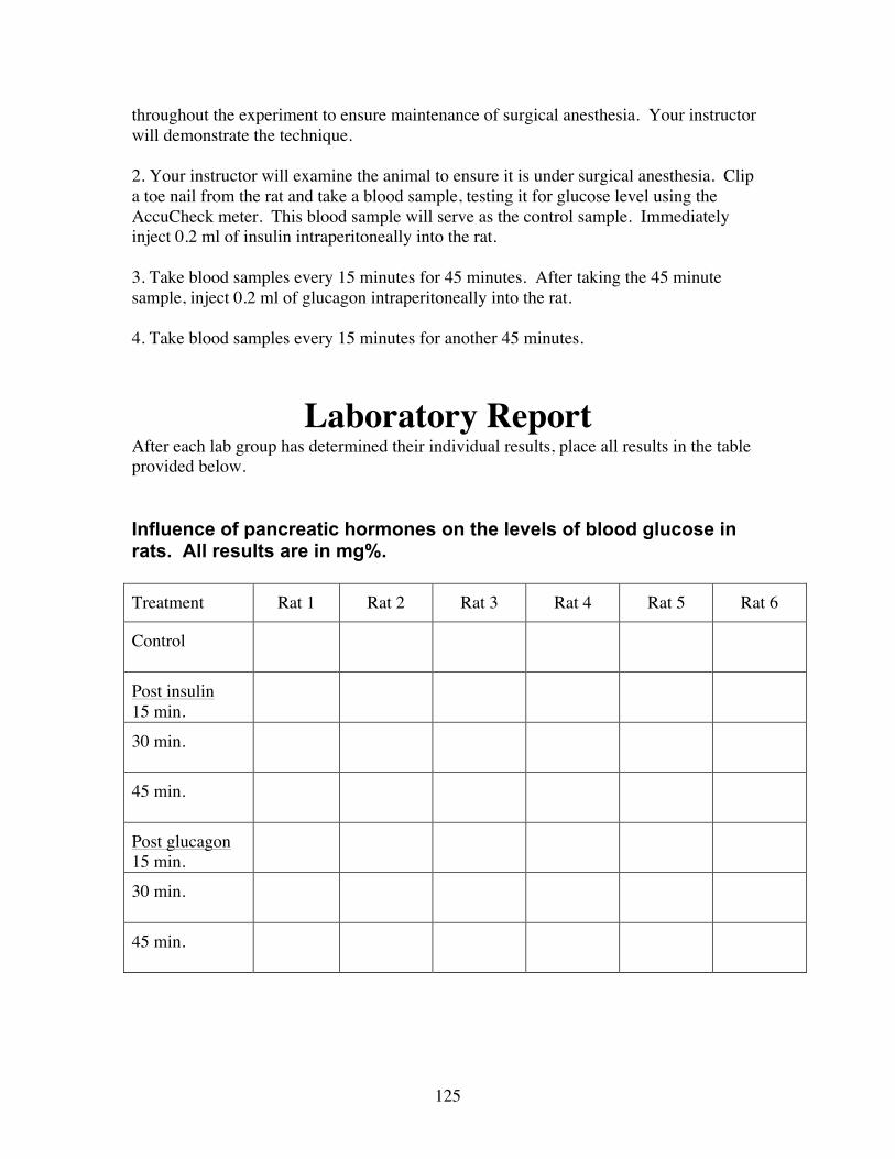
125
throughout the experiment to ensure maintenance of surgical anesthesia. Your instructor will demonstrate the technique. 2. Your instructor will examine the animal to ensure it is under surgical anesthesia. Clip a toe nail from the rat and take a blood sample, testing it for glucose level using the AccuCheck meter. This blood sample will serve as the control sample. Immediately inject 0.2 ml of insulin intraperitoneally into the rat. 3. Take blood samples every 15 minutes for 45 minutes. After taking the 45 minute sample, inject 0.2 ml of glucagon intraperitoneally into the rat. 4. Take blood samples every 15 minutes for another 45 minutes.
Laboratory Report
After each lab group has determined their individual results, place all results in the table provided below. Influence of pancreatic hormones on the levels of blood glucose in rats. All results are in mg%. Treatment Rat 1 Rat 2 Rat 3 Rat 4 Rat 5 Rat 6
Control
Post insulin 15 min.
30 min.
45 min.
Post glucagon 15 min.
30 min.
45 min.

126
Write a one page description of your results, describing the effects of insulin and glucagon and the negative feedback control of endocrine regulation of glucose metabolism.

127
Group projects and oral presentations Introduction The aim of the final two weeks of the laboratory is to provide you with the opportunity to gain experience at A. designing your own experiments, and B. speaking in front of an audience (i.e, the class). You will be asked to design your own experiments based on the information you have gathered throughout the semester. You can choose to perform experiments using the PowerLab or choose something else. The last lab period will be devoted to oral/poster presentations on your findings. Whether your experiments work according to your predications or not does not matter. Your ability to explain why they may not have worked according to your initial hypothesis is important. At the conclusion of the exercise I want you to recognize science for what it is; an imperfect method of gaining information. Prior to conducting your experiments you should consult your laboratory instructor. Guidelines for presentations Each person from the group must speak and outline: A. the purpose of an experiments B. materials used to design and implement the experiments C. the results, and D. what the results mean (i.e., their significance). How your group decides to present your data is up to yourselves. Successful presentations involve meeting frequently as a group, planning and rehearsing as a group, and most importantly - a fair division of labor among group members. Remember, all members of the group will receive the same grade. You may choose to conduct either; A. a poster, or B. a PowerPoint presentation. If you choose to do a poster be aware that you must also present the results orally, guiding your audience through the different aspects of the experiments. Each group must speak for a minimum of 20 minutes and no more than 25 minutes. You will lose points for not adhering to these time restrictions. Each group must be prepared to answer questions from the audience, so be prepared. It may be a good idea to have a list of anticipated questions prepared. Question time will last for about 5 minutes.
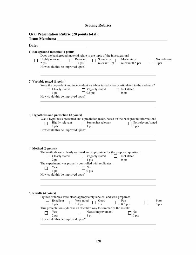
128
Scoring Rubrics Oral Presentation Rubric (20 points total): Team Members:
Date: 1) Background material (2 points)
Does the background material relate to the topic of the investigation? Highly relevant Relevant Somewhat Moderately Not relevant 2 pts 1.5 pts relevant 1 pt relevant 0.5 pts 0 pts
How could this be improved upon? 2) Variable tested (1 point)
Were the dependent and independent variables tested, clearly articulated to the audience? Clearly stated Vaguely stated Not stated 1 pt 0.5 pts 0 pts
How could this be improved upon?
3) Hypothesis and prediction (2 points) Was a hypothesis presented and a prediction made, based on the background information? Highly relevant Somewhat relevant Not relevant/stated 2 pts 1 pt 0 pts
How could this be improved upon?
4) Method (3 points)
The methods were clearly outlined and appropriate for the proposed question: Clearly stated Vaguely stated Not stated 2 pt 1 pts 0 pts
The experiment was properly controlled with replicates: Yes No 1 pt 0 pts
How could this be improved upon?
5) Results (4 points)
Figures or tables were clear, appropriately labeled, and well prepared: Excellent Very good Good Fair Poor 2 pts 1.5 pts 1pt 0.5 pts 0 pts
This presentation style was an effective way to summarize the results: Yes Needs improvement No 2 pts 1 pt 0 pts
How could this be improved upon?
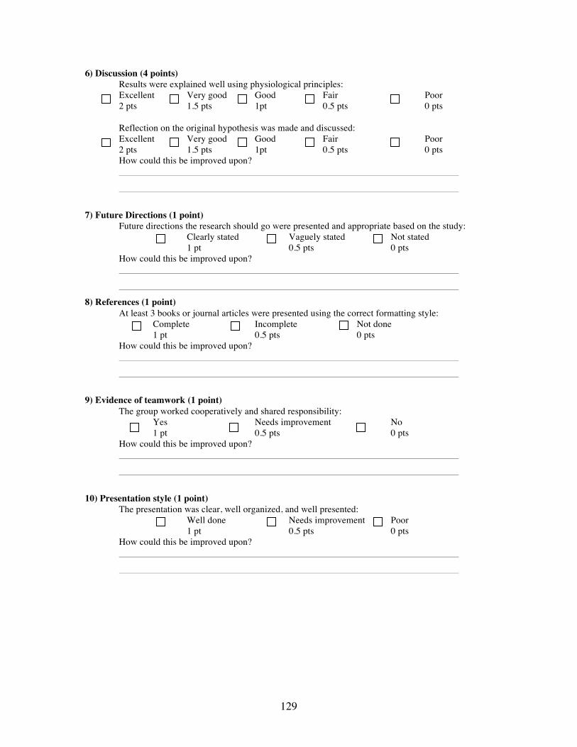
129
6) Discussion (4 points) Results were explained well using physiological principles:
Excellent Very good Good Fair Poor 2 pts 1.5 pts 1pt 0.5 pts 0 pts
Reflection on the original hypothesis was made and discussed: Excellent Very good Good Fair Poor 2 pts 1.5 pts 1pt 0.5 pts 0 pts
How could this be improved upon?
7) Future Directions (1 point)
Future directions the research should go were presented and appropriate based on the study: Clearly stated Vaguely stated Not stated 1 pt 0.5 pts 0 pts
How could this be improved upon?
8) References (1 point) At least 3 books or journal articles were presented using the correct formatting style:
Complete Incomplete Not done 1 pt 0.5 pts 0 pts
How could this be improved upon?
9) Evidence of teamwork (1 point)
The group worked cooperatively and shared responsibility: Yes Needs improvement No 1 pt 0.5 pts 0 pts
How could this be improved upon?
10) Presentation style (1 point)
The presentation was clear, well organized, and well presented: Well done Needs improvement Poor 1 pt 0.5 pts 0 pts
How could this be improved upon?

130
BIO 468 LABORATORY REPORTS -- GRADING RUBRIC
Name: __________________________________ Date __________ 1. Title (1 point)
* Accurate and description of the project __________
2. Abstract (2 points)
* A statement on what was done (0.5) __________
* A statement or two on what methodology was used (0.5) __________
* Main results were outlined (0.5) __________
* Conclusions and significance of the data were mentioned (0.5) __________
3. Introduction (4 points)
* Accurate background information to introduce each
experiment was provided with appropriate references (3) __________
* A statement of purpose was included (1) __________
4. Materials and Methods (2 points)
* Section was written clearly and concisely and referenced (1) __________
* Enough detail was provided to repeat the experiment (1) __________
5. Results (5 points)
* Data from all experiments was included (1) __________
* Tables and figures were clear and well labeled (2) __________
* Tables and figures were used appropriately (1) __________
* Text summarized and accompanied data in table/figures (1) __________
6. Discussion (6 points)
* A brief summary of all key results in first paragraph (1) __________
* Results of each experiment were related back to
information provided in introduction (2) __________
* Physiological mechanism of results explained using references (2) __________
* Success of the experimental design and directions for
future studies were discussed (1) __________
7. References (2 points)
* At least 5 appropriate references were included (1) __________
* References were formatted and cited correctly in the text (1) __________
8. Writing mechanics (3)
* Report was double spaced (1) ___________
* Grammar and spelling were accurate (1) ___________
* Clearly written/ evidence of proof reading (1) ___________
Total Possible Points: 25 Your Score: __________

131
BIO 468/469 INDEPENDENT PROJECT PRESENTATION -- GRADING RUBRIC
Team Members: ______________________________________________________
1. Abstract (2 pts)
* A statement on what was done (0.5) __________
* A statement or two on what methodology was used (0.5) __________
* Main results were outlined (0.5) __________
* The significance of the data were mentioned (0.5) __________
2. Introduction (4 pts)
* Adequate background information to introduce each experiment was provided (including background literature) (3) __________
* A statement of purpose was included at the end (1) __________
3. Materials and Methods (3 pts)
* Enough detail was provided to repeat the experiment (2) __________
* No unnecessary information was provided (1) __________
4. Results (4 pts)
* Tables and figures were legible (1) __________
* Tables and figures were used appropriately (1) __________
* Text summarizes and accompanies data in table/figures (2) __________ 5. Discussion (5 pts)
* A brief summary of key results was presented first (1) __________
* Experiments were discussed in the order in which they appeared in the results (1) __________
* Results of each experiment were related back to information provided in introduction (2) __________
* Success of the experimental design and directions for future studies were discussed (1) __________
6. Style (2 pts)
* Clear and audible voice (1) __________
* Slide presentation well organized with clear slides (1) __________
Total Possible Points: 20 Your Score: __________

132
BIO 468 and 469
LABORATORY NOTEBOOK
GRADING RUBRIC
Name: __________________________________ 1. Well organized and neat. (1 point) __________ 2. Data tables/figures filled in correctly (4 points) __________ 3. All experiments are present and scientific interpretation of the
results (i.e., questions in lab manual) are correct. All questions at end of lab chapters answered (5 points) __________
Total Points Possible: 10 Your Score: __________
Pages where information is either missing, incomplete or incorrect: