Embed Size (px)
Citation preview

EXPERIMENTING WITH A BIGDATA FRAMEWORK FOR SCALINGA DATA QUALITY QUERY SYSTEM
A THESIS SUBMITTED TO THE UNIVERSITY OF MANCHESTER
FOR THE DEGREE OF MASTER OF PHILOSOPHY
IN THE FACULTY OF SCIENCE AND ENGINEERING
2016
BySonia Cisneros Cabrera
School of Computer Science

Contents
Abstract 13
Declaration 14
Copyright 15
Dedication 16
Acknowledgements 17
1 Introduction 181.1 Motivation . . . . . . . . . . . . . . . . . . . . . . . . . . . . . . . . 18
1.2 Research Goals and Contributions . . . . . . . . . . . . . . . . . . . 20
1.3 Research Method . . . . . . . . . . . . . . . . . . . . . . . . . . . . 21
1.4 Thesis Overview . . . . . . . . . . . . . . . . . . . . . . . . . . . . 25
2 Background and Related Work 262.1 Data Quality: Wrangling and the Big Data Life Cycle . . . . . . . . . 26
2.2 Big Data and Parallelism . . . . . . . . . . . . . . . . . . . . . . . . 31
2.3 Big Data Frameworks: Tools and Projects . . . . . . . . . . . . . . . 33
2.3.1 MapReduce, Hadoop and Spark . . . . . . . . . . . . . . . . 35
2.4 Scalability of Data Management Operators . . . . . . . . . . . . . . . 37
3 Designing a Scalable DQ2S 423.1 The Data Quality Query System (DQ2S) . . . . . . . . . . . . . . . . 42
3.1.1 The Framework . . . . . . . . . . . . . . . . . . . . . . . . . 43
3.1.2 The Query . . . . . . . . . . . . . . . . . . . . . . . . . . . 44
3.1.3 The Datasets . . . . . . . . . . . . . . . . . . . . . . . . . . 46
3.1.4 The Algorithms Included in the DQ2S Database Algebra Im-plementation . . . . . . . . . . . . . . . . . . . . . . . . . . 48
2

3.2 The Artifact . . . . . . . . . . . . . . . . . . . . . . . . . . . . . . . 55
3.2.1 The Java DQ2S . . . . . . . . . . . . . . . . . . . . . . . . . 55
3.2.2 The Python DQ2S Implementation . . . . . . . . . . . . . . . 58
3.2.3 The Optimised Python DQ2S Implementation . . . . . . . . . 60
3.2.4 The PySpark DQ2S Implementation . . . . . . . . . . . . . . 62
The Apache Spark Generals . . . . . . . . . . . . . . . . . . 62
Spark Python API . . . . . . . . . . . . . . . . . . . . . . . 67
3.3 Summary . . . . . . . . . . . . . . . . . . . . . . . . . . . . . . . . 70
4 Experiment design 714.1 Objectives and Scope of the Experiment . . . . . . . . . . . . . . . . 72
4.2 Data and Tools . . . . . . . . . . . . . . . . . . . . . . . . . . . . . 74
4.3 Setup: Spark Cluster and Application Settings . . . . . . . . . . . . . 76
4.3.1 The Apache Spark Local Mode . . . . . . . . . . . . . . . . 76
4.3.2 The Apache Spark Standalone Mode . . . . . . . . . . . . . . 77
4.4 Experiment Procedure . . . . . . . . . . . . . . . . . . . . . . . . . 79
4.5 Algorithm Comparison . . . . . . . . . . . . . . . . . . . . . . . . . 90
4.6 Experiment Evaluation . . . . . . . . . . . . . . . . . . . . . . . . . 92
4.6.1 Performance Metrics . . . . . . . . . . . . . . . . . . . . . . 92
4.6.2 Validity Evaluation . . . . . . . . . . . . . . . . . . . . . . . 94
4.7 Summary . . . . . . . . . . . . . . . . . . . . . . . . . . . . . . . . 99
5 Evaluation of Experimental Results 1005.1 Experiments Results . . . . . . . . . . . . . . . . . . . . . . . . . . 100
5.2 Algorithm Comparison . . . . . . . . . . . . . . . . . . . . . . . . . 118
5.3 Summary . . . . . . . . . . . . . . . . . . . . . . . . . . . . . . . . 139
6 Conclusions and Future Work 1406.1 Research Summary and Key Results . . . . . . . . . . . . . . . . . . 140
6.2 Research Contributions and Impact . . . . . . . . . . . . . . . . . . . 141
6.3 Future Work . . . . . . . . . . . . . . . . . . . . . . . . . . . . . . . 142
Bibliography 146
A DQ2S Source code 162A.1 The Java DQ2S . . . . . . . . . . . . . . . . . . . . . . . . . . . . . 162
A.2 The Python DQ2S . . . . . . . . . . . . . . . . . . . . . . . . . . . . 175
3

A.3 The Optimised Python DQ2S . . . . . . . . . . . . . . . . . . . . . . 186A.4 The PySpark DQ2S . . . . . . . . . . . . . . . . . . . . . . . . . . . 191
B Apache Spark set up 198B.1 Configuration of Spark’s Basic Elements . . . . . . . . . . . . . . . . 198B.2 Single Machine Deployment . . . . . . . . . . . . . . . . . . . . . . 199B.3 PySpark Submission to the DPSF Cluster . . . . . . . . . . . . . . . 201
C Testing Results 205C.1 Raw Results . . . . . . . . . . . . . . . . . . . . . . . . . . . . . . . 205C.2 Performance Metrics Results . . . . . . . . . . . . . . . . . . . . . . 224
D Apache Spark User Level Proposal 227
Word Count: 37 242
4

List of Tables
1.1 The Design Science Research guideliness . . . . . . . . . . . . . . . 23
2.1 Big data life cycle processes definitions. . . . . . . . . . . . . . . . . 30
2.2 Big data frameworks available for data quality tasks . . . . . . . . . . 34
2.3 Summary of the most relevant state-of-the-art related studies. . . . . . 41
3.1 Operators comprising the DQ2S Timeliness query. . . . . . . . . . . . 50
3.2 Java DQ2S technical description . . . . . . . . . . . . . . . . . . . . 58
3.3 Python DQ2S technical description . . . . . . . . . . . . . . . . . . . 60
3.4 Optimised Python DQ2S technical description . . . . . . . . . . . . . 62
3.5 PySpark DQ2S technical description. . . . . . . . . . . . . . . . . . . 70
4.1 Research Question’s solution plan . . . . . . . . . . . . . . . . . . . 73
4.2 Relation of number of rows and size per each input dataset utilised inthe experimentation. . . . . . . . . . . . . . . . . . . . . . . . . . . 74
4.3 Hardware specification of the desktop machine (PC) and the cluster(DPSF) utilised in the experimentation. . . . . . . . . . . . . . . . . 75
4.4 Tools used in the empirical evaluation of the research . . . . . . . . . 76
4.5 Spark configuration locations . . . . . . . . . . . . . . . . . . . . . . 79
4.6 General overview of the experiment’s aim . . . . . . . . . . . . . . . 79
4.7 Number of runtimes and averages collected by experiment. . . . . . . 80
4.8 Conclusion validity threats applicable to the research presented. De-tails and addressing approach. . . . . . . . . . . . . . . . . . . . . . 96
4.9 Internal validity threats applicable to the research presented. Detailsand addressing approach. . . . . . . . . . . . . . . . . . . . . . . . . 97
4.10 Construct validity threats applicable to the research presented. Detailsand addressing approach. . . . . . . . . . . . . . . . . . . . . . . . . 98
4.11 External validity threats applicable to the research presented. Detailsand addressing approach. . . . . . . . . . . . . . . . . . . . . . . . . 99
5

5.1 Relation of the dataset sizes and results when executing OptimisedPython DQ2S in a single machine for Experiment 4. . . . . . . . . . . 104
5.2 Size in bytes for the first dataset that caused a failure (12 000 000rows), and the maximum number of rows processed by the OptimisedPython DQ2S (11 500 000). . . . . . . . . . . . . . . . . . . . . . . . 104
5.3 Relation of seconds decreased from different configurations using 1worker (W) and 1 to 4 cores (C) with the Standalone mode in a singlemachine. . . . . . . . . . . . . . . . . . . . . . . . . . . . . . . . . . 108
5.4 Times Slower: Relation between the runtime results of the PySpark in-stance with 1 (sequential) and 8 threads (best time). Where local[1]<local[8]
indicates the PySpark DQ2S in local mode with 8 threads is slower thanthe same implementation with 8 threads as many times as indicated. . 111
5.5 Size in GB for the datasets sizes processed on the cluster. . . . . . . . 115
5.6 Relation of the dataset sizes and results when executing the OptimisedPython DQ2S in the cluster for Experiment 9. . . . . . . . . . . . . . 117
5.7 Times Slower: Relation between Original Java and Python runtimeresults. Where Python <Java indicates the Python DQ2S is slowerthan the Java implementation as many times as indicated. . . . . . . . 118
5.8 Times Slower: Relation between Python and Optimised Python run-time results. Where Python <Optimised Python indicates the PythonDQ2S is slower than the Optimised Python implementation as manytimes as indicated. . . . . . . . . . . . . . . . . . . . . . . . . . . . . 122
5.9 Times Slower: Relation between Original Java and Optimised Pythonruntime results. Where Java <Optimised Python indicates the JavaDQ2S is slower than the Optimised Python implementation as manytimes as indicated. . . . . . . . . . . . . . . . . . . . . . . . . . . . . 122
5.10 Times Slower: Relation between the runtime results of the OptimisedPython and PySpark with 1 thread. Where local[1]<Optimised Python
indicates the PySpark DQ2S in local mode with 1 thread is slower thanthe Optimised implementation as many times as indicated. . . . . . . 124
5.11 Times Slower: Relation between the runtime results of the OptimisedPython and PySpark with 8 threads. Where local[8]<Optimised Python
indicates the PySpark DQ2S in local mode with 8 threads is slower thanthe Optimised implementation as many times as indicated. . . . . . . 124
6

5.12 Times Slower: Relation between the runtime results of the OptimisedPython and PySpark with 1 and 8 threads for 11 500 000 rows. Wherethe notation implementation <implementation indicates the left im-plementation is slower than the implementation on the right as manytimes as indicated. . . . . . . . . . . . . . . . . . . . . . . . . . . . . 126
B.1 Apache Spark processes’ default values for Standalone mode, whereNA stands for “Not Applicable”. . . . . . . . . . . . . . . . . . . . . 198
B.2 Apache Spark processes’ general configuration parameters and loca-tion, where NA stands for “Not Applicable”. . . . . . . . . . . . . . . 199
C.1 Original Java DQ2S execution times. . . . . . . . . . . . . . . . . . . 209
C.2 Python DQ2S execution times. . . . . . . . . . . . . . . . . . . . . . 210
C.3 Optimised Python DQ2S execution times. . . . . . . . . . . . . . . . 210
C.4 Optimised Python DQ2S execution times in nanoseconds and secondsfor 11 500 000 rows. . . . . . . . . . . . . . . . . . . . . . . . . . . 211
C.5 Execution times obtained from PySpark DQ2S Standalone mode in asingle machine over 1 worker and 1 core. . . . . . . . . . . . . . . . 211
C.6 Execution times obtained from PySpark DQ2S Standalone mode in asingle machine over 1 worker and 2 cores each one. . . . . . . . . . . 212
C.7 Execution times obtained from PySpark DQ2S Standalone mode in asingle machine over 1 worker and 3 cores each one. . . . . . . . . . . 212
C.8 Execution times obtained from PySpark DQ2S Standalone mode in asingle machine over 1 worker and 4 cores each one. . . . . . . . . . . 213
C.9 Execution times obtained from PySpark DQ2S Standalone mode in asingle machine over 2 workers and 1 core each one. . . . . . . . . . . 213
C.10 Execution times obtained from PySpark DQ2S Standalone mode in asingle machine over 2 workers and 2 cores each one. . . . . . . . . . 214
C.11 Execution times obtained from PySpark DQ2S Standalone mode in asingle machine over 3 workers and 1 core each one. . . . . . . . . . . 214
C.12 Execution times obtained from PySpark DQ2S Standalone mode in asingle machine over 4 workers and 1 core each one. . . . . . . . . . . 215
C.13 Execution times obtained from PySpark DQ2S Local mode using 1core in a single machine. . . . . . . . . . . . . . . . . . . . . . . . . 215
C.14 Execution times obtained from PySpark DQ2S Local mode using 2cores in a single machine. . . . . . . . . . . . . . . . . . . . . . . . . 216
7
C.15 Execution times obtained from PySpark DQ2S Local mode using 3cores in a single machine. . . . . . . . . . . . . . . . . . . . . . . . . 216
C.16 Execution times obtained from PySpark DQ2S Local mode using 4cores in a single machine. . . . . . . . . . . . . . . . . . . . . . . . . 217
C.17 Execution times obtained from PySpark DQ2S Local mode using 5cores in a single machine. . . . . . . . . . . . . . . . . . . . . . . . . 218
C.18 Execution times obtained from PySpark DQ2S Local mode using 6cores in a single machine. . . . . . . . . . . . . . . . . . . . . . . . . 218
C.19 Execution times obtained from PySpark DQ2S Local mode using 7cores in a single machine. . . . . . . . . . . . . . . . . . . . . . . . . 219
C.20 Execution times obtained from PySpark DQ2S Local mode using 8cores in a single machine. . . . . . . . . . . . . . . . . . . . . . . . . 219
C.21 Execution times obtained from PySpark DQ2S Local mode using 1 to6 cores in a single machine for 11 500 000 rows. . . . . . . . . . . . . 220
C.22 Execution times obtained from PySpark DQ2S Local mode using 7 to10 cores in a single machine for 11 500 000 rows. . . . . . . . . . . . 220
C.23 Execution times obtained from PySpark DQ2S Local mode using 1 to6 cores in a single machine for 35 000 000 rows. . . . . . . . . . . . . 221
C.24 Execution times obtained from PySpark DQ2S Local mode using 7 to10, 12, and 16 cores in a single machine for 35 000 000 rows. . . . . . 221
C.25 Execution times obtained from PySpark DQ2S Standalone mode pro-cessing 35 000 000 rows with 1 to 4 worker nodes on a cluster. . . . . 222
C.26 Execution times obtained from PySpark DQ2S Standalone mode pro-cessing 70 000 000 rows with 1 to 4 worker nodes on a cluster. . . . . 222
C.27 Execution times obtained from PySpark DQ2S Standalone mode pro-cessing 105 000 000 rows with 1 to 4 worker nodes on a cluster. . . . 223
C.28 Optimised Python DQ2S execution times in nanoseconds and secondsfor 35 000 000 rows. . . . . . . . . . . . . . . . . . . . . . . . . . . 223
C.29 Performance Metrics for Parallel Algorithms: Values calculated for11 500 000 rows processing from PySpark Local mode in single ma-chine execution. . . . . . . . . . . . . . . . . . . . . . . . . . . . . . 225
C.30 Performance Metrics for Parallel Algorithms: Values calculated fromPySpark Standalone mode in single machine execution. . . . . . . . . 225
C.31 Performance Metrics for Parallel Algorithms: Values calculated fromPySpark Local mode in single machine execution. . . . . . . . . . . . 226
8

List of Figures
1.1 The Design Science General Process . . . . . . . . . . . . . . . . . . 22
2.1 The big data life cycle . . . . . . . . . . . . . . . . . . . . . . . . . 27
3.1 Timeliness query expressed with DQ2L [26]. . . . . . . . . . . . . . 46
3.2 Timeliness query expressed with SQL [26]. . . . . . . . . . . . . . . 46
3.3 OrderT dataset’s first 9 rows. . . . . . . . . . . . . . . . . . . . . . . 46
3.4 StatusTimelinessQR dataset’s first 9 rows. . . . . . . . . . . . . . . . 46
3.5 General sequence diagram for the Timeliness query, build from theJava DQ2S instance. . . . . . . . . . . . . . . . . . . . . . . . . . . . 51
3.6 Class diagram for the Java DQ2S engine. . . . . . . . . . . . . . . . . 52
4.1 Flow structure of Chapter 4 . . . . . . . . . . . . . . . . . . . . . . . 71
5.1 Runtime registered in seconds for the Original Java DQ2S processing50 000, 100 000 and 1 000 000 rows. . . . . . . . . . . . . . . . . . . 101
5.2 Runtime registered in seconds for the Python DQ2S processing 50 000,100 000 and 1 000 000 rows. . . . . . . . . . . . . . . . . . . . . . . 102
5.3 Runtime registered in seconds for the Optimised Python DQ2S pro-cessing 50 000, 100 000 and 1 000 000 rows. . . . . . . . . . . . . . 103
5.4 Runtime registered in seconds for the PySpark DQ2S processing 50 000,100 000 and 1 000 000 rows in Standalone mode implemented in a sin-gle machine, where W refers to workers and C to cores in the ApacheSpark definition. The marked line indicates the lower runtime obtainedper dataset size. . . . . . . . . . . . . . . . . . . . . . . . . . . . . . 107
5.5 Runtime registered in seconds for the PySpark DQ2S processing 50 000,100 000 and 1 000 000 rows in Local mode implemented in a singlemachine. The marked line indicates the lower runtime obtained perdataset size. . . . . . . . . . . . . . . . . . . . . . . . . . . . . . . . 109
9

5.6 Runtime registered in seconds for the PySpark DQ2S processing 50 000rows in Local mode implemented in a single machine. . . . . . . . . . 109
5.7 Runtime registered in seconds for the PySpark DQ2S processing 100 000rows in Local mode implemented in a single machine. . . . . . . . . . 110
5.8 Runtime registered in seconds for the PySpark DQ2S processing 1 000 000rows in Local mode implemented in a single machine. . . . . . . . . . 110
5.9 Runtime registered in seconds for the PySpark DQ2S processing 11 500 000and 35 000 000 rows in Local mode implemented in a single machine.The marked line indicates the lower runtime obtained per dataset size. 112
5.10 Runtime registered in seconds for the PySpark DQ2S processing 11 500 000rows in Local mode implemented in a single machine. . . . . . . . . . 113
5.11 Runtime registered in seconds for the PySpark DQ2S processing 35 000 000rows in Local mode implemented in a single machine. . . . . . . . . . 113
5.12 Runtime registered in seconds for the processing of 35 000 000, 70 000 000,and 105 000 000 rows with PySpark DQ2S in Standalone mode usedin a cluster, utilising from 1 to 4 nodes (worker nodes). Each node wasconfigured to contain 1 worker process with 8 executors, each executorwith 2 cores and 32GB of available memory. . . . . . . . . . . . . . . 115
5.13 Comparison of the runtime in seconds obtained when processing 50 000rows with the non-big data instances. . . . . . . . . . . . . . . . . . . 120
5.14 Comparison of the runtime in seconds obtained when processing 100 000rows with the non-big data instances. . . . . . . . . . . . . . . . . . . 121
5.15 Comparison of the runtime in seconds obtained when processing 1 000 000rows with the non-big data instances. . . . . . . . . . . . . . . . . . . 121
5.16 Comparison of the runtime in seconds obtained when processing 50 000,100 000 and 1 000 000 rows with the best non-big data instance (se-quential) and its implementation with a big data instance using 1 and8 threads . . . . . . . . . . . . . . . . . . . . . . . . . . . . . . . . . 123
5.17 Comparison of the runtime in seconds obtained when processing 11 500 000rows with the best non-big data instance and the PySpark one with 1and 8 threads. . . . . . . . . . . . . . . . . . . . . . . . . . . . . . . 126
5.18 Ideal Speedup compared against the speedup results obtained from thePySpark DQ2S Local mode in a single machine. . . . . . . . . . . . . 127
5.19 Ideal Efficiency compared against the speedup results obtained fromthe PySpark DQ2S Local mode in a single machine. . . . . . . . . . . 127
10

5.20 Performance Metrics for Parallel Algorithms: Values calculated for11 500 000 rows processing for the PySpark Local mode DQ2S in-stance. Where green represents the higher speedup and efficiencyobtained, yellow and orange represent intermediate speedup and ef-ficiency values, and red indicates the configurations that obtained thelowest speedup and efficiency considering the values calculated for allof the configurations. . . . . . . . . . . . . . . . . . . . . . . . . . . 128
5.21 Runtime in seconds for the PySpark DQ2S with Standalone and Localmode, handling from 1 to 4 tasks simultaneously for 50 000 rows. . . 130
5.22 Runtime in seconds for the PySpark DQ2S with Standalone and Localmode, handling from 1 to 4 tasks simultaneously for 100 000 rows. . . 131
5.23 Runtime in seconds for the PySpark DQ2S with Standalone and Localmode, handling from 1 to 4 tasks simultaneously for 1 000 000 rows. . 131
5.24 Difference in seconds for 50 000, 100 000 and 100 000 rows whenexecuting the PySpark DQ2S with Standalone and Local mode, whereLocal mode was the quickest for all of the three dataset sizes. . . . . . 132
5.25 Speedup and Efficiency individual heat map for the Standalone and Lo-cal mode PySpark DQ2S.Where green represents the higher speedupand efficiency obtained, yellow and orange represent intermediate speedupand efficiency values, and red indicates the configurations that obtainedthe lowest speedup and efficiency considering the values calculated forall of the configurations within each set of tables. . . . . . . . . . . . 133
5.26 Speedup and Efficiency global heat map for the Standalone and Localmode PySpark DQ2S.Where green represents the higher speedup andefficiency obtained, yellow and orange represent intermediate speedupand efficiency values, and red indicates the configurations that obtainedthe lowest speedup and efficiency considering the values calculated forall of the configurations of all of the tables. . . . . . . . . . . . . . . 133
5.27 Runtimes obtained from the execution of the Timeliness query with35 000 000 rows datasets, for PySpark in a single machine with Localmode and a Standalone mode in a cluster (DPSF). . . . . . . . . . . . 134
5.28 Runtime in seconds for 35 000 000 rows processed in the DPSF clusterwith the Optimised Python DQ2S and the PySpark instance in Stan-dalone mode. . . . . . . . . . . . . . . . . . . . . . . . . . . . . . . 135
11

D.1 Proposed big data frameworks user classification with regards to expe-rience and expertise. . . . . . . . . . . . . . . . . . . . . . . . . . . 227
12

Abstract
EXPERIMENTING WITH A BIG DATA FRAMEWORK FOR SCALING A
DATA QUALITY QUERY SYSTEM
Sonia Cisneros CabreraA thesis submitted to The University of Manchester
for the degree of Master of Philosophy, 2016
The work presented in this thesis comprises the design, implementation and evalu-ation of extensions made to the Data Quality Query System (DQ2S), a state-of-the-artdata quality-aware query processing framework and query language, towards testingand improving its scalability when working with increasing amounts of data. The pur-pose of the evaluation is to assess to what extent a big data framework, such as ApacheSpark, can offer significant gains in performance, including runtime, required amountof memory, processing capacity, and resource utilisation, when running over differentenvironments. DQ2S enables assessing and improving data quality within informa-tion management by facilitating profiling of the data in use, and leading to the supportof data cleansing tasks, which represent an important step in the big data life-cycle.Despite this, DQ2S, as the majority of data quality management systems, is not de-signed to process very large amounts of data. This research describes the journey ofhow data quality extensions from an earlier implementation that processed two datasetswith 50 000 rows each one in 397 seconds, were designed, implemented and tested toachieve a big data solution capable of processing 105 000 000 rows in 145 seconds.The research described in this thesis provides a detailed account of the experimen-tal journey followed to extend DQ2S towards exploring the capabilities of a popularbig data framework (Apache Spark), including the experiments used to measure thescalability and usefulness of the approach. The study also provides a roadmap forresearchers interested in re-purposing and porting existing information managementsystems and tools to explore the capabilities provided by big data frameworks, par-ticularly useful given that re-purposing and re-writing existing software to work withbig data frameworks is a less costly and risky approach when compared to greenfieldengineering of information management systems and tools.
13

Declaration
No portion of the work referred to in this thesis has beensubmitted in support of an application for another degree orqualification of this or any other university or other instituteof learning.
14
Copyright
i. The author of this thesis (including any appendices and/or schedules to this the-sis) owns certain copyright or related rights in it (the “Copyright”) and s/he hasgiven The University of Manchester certain rights to use such Copyright, includ-ing for administrative purposes.
ii. Copies of this thesis, either in full or in extracts and whether in hard or electroniccopy, may be made only in accordance with the Copyright, Designs and PatentsAct 1988 (as amended) and regulations issued under it or, where appropriate,in accordance with licensing agreements which the University has from time totime. This page must form part of any such copies made.
iii. The ownership of certain Copyright, patents, designs, trade marks and other in-tellectual property (the “Intellectual Property”) and any reproductions of copy-right works in the thesis, for example graphs and tables (“Reproductions”), whichmay be described in this thesis, may not be owned by the author and may beowned by third parties. Such Intellectual Property and Reproductions cannotand must not be made available for use without the prior written permission ofthe owner(s) of the relevant Intellectual Property and/or Reproductions.
iv. Further information on the conditions under which disclosure, publication andcommercialisation of this thesis, the Copyright and any Intellectual Propertyand/or Reproductions described in it may take place is available in the Univer-sity IP Policy (see http://documents.manchester.ac.uk/display.aspx?
DocID=24420), in any relevant Thesis restriction declarations deposited in theUniversity Library, The University Library’s regulations (see http://www.library.manchester.ac.uk/about/regulations/) and in The University’s policy onpresentation of Theses.
15

Dedication
To my husband, my parents, and my four grandparents.
16

Acknowledgements
“If I have seen further it is by
standing on the shoulders of Giants.”
— Isaac Newton
I would like to thank my supervisors Sandra Sampaio, and Pedro Sampaio, whosesupport and guidance allowed me to pursue my own path, with the confidence of havingwide and kind open doors whenever I faced doubts and confusion. I am deeply gratefulto them for encouraging me to keep going, and to keep growing.
I am thankful to the Research Infrastructure Team within Research IT at The Uni-versity of Manchester, for their tireless technical support towards the Data ProcessingShared Facility cluster being able to work with Apache Spark, special thanks to GeorgeLeaver, Penny Richardson, and Anja Le Blanc.
I met wonderful people during my studies at the School of Computer Science, staff,fellow students, professors and graduates, who made me feel incredibly fortunate tocoincide with them in this time and place since the first time I arrived to the Universityof Manchester. I am particularly grateful to Michele Filannino, and Oscar Flores-Vargas for showing me the passion and kindness of providing academic support andshare their expertise to others, including me.
I also would like to thank Jessica Cueva, Atenea Manzano, and Estrella Armenta,for their support given during the process of my enrolment to the University of Manch-ester, a very important and crucial phase to make this work happen. Thanks for inspir-ing me to dream big.
I owe a lifetime debt of gratitude to Jesus Carmona-Sanchez, Delphine Dourdou,and Lily Carmona, for being the family Manchester gave me.
And last, but not least, I want to thank my sponsor, the National Council on Scienceand Technology of Mexico (CONACyT for its acronym in Spanish), for giving me theopportunity and funding to study a Master’s degree at the University of Manchester.
17

Chapter 1
Introduction
The work presented in this thesis aims to design, implement and evaluate extensions tothe Data Quality Query System (DQ2S) [26], a quality-aware query processing frame-work and query language, towards leveraging the Apache Spark big data framework.This study sets out to investigate the usefulness of it towards scalability for processingdata quality techniques by converting a current successful algorithm into a big datacapable one. The purpose of the evaluation is to assess to what extent a big data frame-work offers significant gains in performance (runtime, memory required, processingcapacity, resource utilisation), maintaining the same levels of data quality that an algo-rithm executed without using the big data framework.
1.1 Motivation
Data appears to be one of the most valuable assets of organisations in the digital era[59, 91, 120] , probably due to the power of the information provided by it, as LucianoFloridi and Phyllis Illiari mention, “The most developed post-industrial societies liveby information, and Information and Communication Technologies (ICTs) keep themoxygenated” [42].
The importance of data could also be weighted by looking to the efforts done glob-ally to protect data, to improve its management or to get a better understanding of it.An example of this can be found in the International Organization for Standardization(ISO) norm for Information Security Management (ISO/IEC 27001), which gives theguidelines and certifiable best practices regarding information, and therefore data, con-sidering it as a valuable asset within organisations. Another example could be found inthe recognised best practices in information technology management services, such as
18

1.1. MOTIVATION 19
The Information Technology Infrastructure Library (ITIL), which grew based on theclaim that information is a pillar of business and not a separate part of it [13].
Nowadays, data is not only created by companies, but by individuals. For example,while walking on a street that has a sensor, sending out a text message, writing anemail or even just turning on an internet connected television and watching a show;all of those actions generate data in one or another way. It is said that in 2013, morethan 90% of the worldwide amount of data had appeared just in the biennium before[22, 36, 60] and it had kept on growing, making an estimate of “40 Zettabytes of datacreated by 2020” [58].
It is so easy to generate data, that storage and processing technologies are runningout of capacity to cope with demand. The concept “big data” refers not only to largeamounts of data in terms of storage size (Volume), but to its inherent characteristic ofbeing created very fast (Velocity), its uncontrollable nature of heterogeneity (Variety)[58], its measurable degree of accuracy (Veracity), and its potential to unveil relevantinsights (Value) [58, 82]. Thus, new technologies capable of handling big data areessential to the future of information technology.
One of the most important characteristics of big data is the value that could beretrieved from it, even into a level of obtaining information that was not known aboutits existence beforehand. For instance, the data gathered from an engine of commercialairplanes, with around 5 000 factors being monitored, can generate predictions onfailures, or even make prognosis about turbulence based on forecast provided by thesame data. In this sense, by analysing the information produced by sensors it is possibleto generate savings of more than 30 million USD for airlines with this technology,by helping them to reduce costs and extend usage of their planes as a result of theinsight obtained by the large amount of data that sensors provided[9], in this case, thecollection of the big data from the airplanes’ engines leads to important information tobe used in several contexts.
Back in 2009, a system built by Google, helped to solve health issues in the UnitedStates of America (USA) when H1N1 virus was being spread presumably as a pan-demic infection, in which situation, to know about new cases as fast as possible wascrucial to keep the spreading under control. Google made this by looking at people’squeries on the Internet, gathering more than a billion every day, and finding correla-tions between the frequency of certain search queries and the spread of flu over timeand space. This system found combinations of 45 search terms among the 50 000 000most popular searched ones, ending in a system that was able to predict a new case of
20 CHAPTER 1. INTRODUCTION
infection. That helped to slow the spread by enabling health authorities to take actionin almost real-time. [83]. This is an example of the power of big data to provide societywith useful insights.
A large volume of data creates the need for higher capacity storage machines andmore powerful processors, as well as the concern about the quality of data in termsof completeness, consistency, uniqueness, timeliness, validity and accuracy (Veracity):the core data quality dimensions [7, 58]. Low data quality represents a problem forintegration, visualisation, and analysis, which could be identified as a significant diffi-culty to utilise the data, and whether it is in small scale or big data, poor quality couldlead to making severe and costly decisions [12].
It could be said that a large volume of data itself is not a warranty of better valuethan few data. The quality of data represents an important factor to be considered whenmaking this assumption, for instance, cancer treatments include medication which hasits proved effectiveness by the results of testing made on the participant patient’s DNA,so, when a doctor chooses a medication for a given patient, both have to hope thatsimilarity between DNAs is close enough to those who participated in the drug trials[83], based on that premise, Steve Jobs decided to get a more personal treatment, byrequesting his complete genetic code, not only a part of it [83] so the cancer medicationcould be the most precise therapy, aiming at extending his life for some years. Thisis an example in which, even though it was not a sample but the whole information, asingle error would have had serious consequences: big data needs to be quality data.
Big data frameworks appeared as “the solution” to the big data problem, providingscalability, speedup and the possibility to compute big data despite its heterogeneityand high volume characteristics. Accompanied by its related storing technologies, bigdata frameworks have been considered as the most suitable option to compute largevolumes of data, replacing Message Passing Interface (MPI) traditional technologies,parallel and distributed programming as former approaches. With the growth thisframeworks have been presenting lately, it is of interest to analyse its application todata quality, and therefore explore if a big data framework can provide a solution forthis area too.
1.2 Research Goals and Contributions
This research covers the design, implementation and evaluation of some of the algo-rithms included in the DQ2S towards increasing volume of data handled and speed

1.3. RESEARCH METHOD 21
of processing using a big data framework, seeking performance improvements suchas memory required, processing capacity and resource utilisation compared to its us-age without the framework. The interest of the research relies on providing scalable,cost-effective, highly-automated, and optimised solutions.
The research requires redesigning the selected algorithms towards developing aversion using big data technologies, so the following objectives can be met:
• Examine the potential gains in performance and scalability with the applicationof a big data framework.
• Explore the different parametrisations of the big data framework constructs toassess the impact on data quality algorithms.
• Propose changes to data quality methods and techniques based on the use of bigdata.
• Perform a literature review of the main big data frameworks and its environ-ments, classified by purpose of usage.
• Conduct an exploratory empirical evaluation of the set of algorithms imple-mented using the selected big data framework, from a software engineering per-spective.
This study can be used as a guide to extend data quality algorithms to increaseperformance and make them available to be used with larger datasets. The approachwill also contribute to the literature by providing insights on key decisions to extend asequential algorithm to benefit from parallelism using the Apache Spark ApplicationProgramming Interface (API).
1.3 Research Method
The research will be supported and developed based on the methodology known as“Design Science Research”, applicable for Information Systems Research. Consider-ing that this study fits well into that category when recognising that, according to theUnited Kingdom Academy for Information Systems (UKAIS), the information pro-cessing supported by technologies is part of the definition of Information Systems(IS), having as study field the area related to those technologies that provide gainsto the IS progress towards society and organisations [139]. Besides, this research is
22 CHAPTER 1. INTRODUCTION
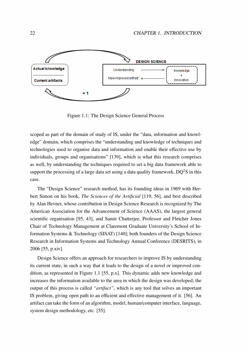
Figure 1.1: The Design Science General Process
scoped as part of the domain of study of IS, under the “data, information and knowl-edge” domain, which comprises the “understanding and knowledge of techniques andtechnologies used to organise data and information and enable their effective use byindividuals, groups and organisations” [139], which is what this research comprisesas well, by understanding the techniques required to set a big data framework able tosupport the processing of a large data set using a data quality framework, DQ2S in thiscase.
The “Design Science” research method, has its founding ideas in 1969 with Her-bert Simon on his book, The Sciences of the Artificial [119, 56], and best describedby Alan Hevner, whose contribution in Design Science Research is recognized by TheAmerican Association for the Advancement of Science (AAAS), the largest generalscientific organisation [95, 43], and Samir Chatterjee, Professor and Fletcher JonesChair of Technology Management at Claremont Graduate University’s School of In-formation Systems & Technology (SISAT) [140]; both founders of the Design ScienceResearch in Information Systems and Technology Annual Conference (DESRITS), in2006 [55, p.xiv].
Design Science offers an approach for researchers to improve IS by understandingits current state, in such a way that it leads to the design of a novel or improved con-dition, as represented in Figure 1.1 [55, p.x]. This dynamic adds new knowledge andincreases the information available to the area in which the design was developed; theoutput of this process is called “artifact”, which is any tool that solves an importantIS problem, giving open path to an efficient and effective management of it. [56]. Anartifact can take the form of an algorithm, model, human/computer interface, language,system design methodology, etc. [55].

1.3. RESEARCH METHOD 23
Guideline Description1: Design as an Artifact Design-science research in this study, leads to the
creation of an artifact in the form of a set of al-gorithms implemented within the Apache Sparkframework using the Python API, which comprisean extension to the DQ2S current algebra operationalgorithms, described in Section 3.2.4
2: Problem Relevance This study comprises the development oftechnology-based solutions to the data qual-ity requirement of big data, with its relevancementioned in Section 1.1.
3: Design Evaluation The evaluation phase supports the constructionphase towards the quality of the design process ofthe artifact. Several evaluations were performed,according to the research method described in thepresent section.
4: Research Contributions Contributions to knowledge will be added to thedata quality area, as well as the big data IS, as pre-sented in Section 1.2.
5: Research Rigor The utility of the artifact to support the objectivesof this research, as well as its efficacy handling bigdata, will be assessed according to the EvaluationMethod, described in Chapter 4.
6: Design as a Search Process As part of the iterative search process, as describedin Chapter 4 and presented in Chapter 5, an opti-mised version was also studied and implemented.
7: Communication of Research The research outcomes and results will be commu-nicated to the community through the most suit-able way according to the results, both to technol-ogy and management oriented audiences.
Table 1.1: The Design Science Research guideliness

24 CHAPTER 1. INTRODUCTION
The methodology proposes 7 guidelines that will be followed in the developmentof the research. A summary of the main concept of the guidelines applied to the studyis shown in Table 1.1, according to the guides presented in [55] and described below.
In order to test if a big data framework offers significant gain in performance (runtime, memory required, processing capacity, and resource utilisation) maintaining thesame levels of data quality that an algorithm executed without it, and according to theDesign Science Research Method, the DQ2S will be extended to an implementationusing Apache Spark technologies. This implementation will conform the IT artifact,created to address the need of organisations to handle big data and to have high qualitydata. These scalable set of algorithms will be described widely, including the con-structs, models and methods applied in the development of them, enabling its imple-mentation and application in an appropriate domain, considering that the IT artifact isthe core subject matter [55].
A Design Evaluation plan was executed to demonstrate the utility, quality and effi-cacy of the scalable algorithms rigorously. This evaluation will be performed in phases,comprising Testing, Analytical, Experimental, and Descriptive Evaluation Methods[55].
The first evaluation will assure that the set-up of the original algorithms, configuredin the machine available to develop the research is made correctly so it fulfils theexpected results, according to its original model. This evaluation is expected to identifyfailures and misbehaviours, leading to its mending in order to have the proper outputand unbiased performance measures. For the analytical evaluation, the structure ofthe algorithms will be examined, using pseudocode to describe them and later basedon the research results, performance metrics for each algorithm will be produced. Aspart of the experimental evaluation, a case study within an e-Business context will beset in which the scalable algorithms will solve the case and point out its qualities insolving the case, which will be related to the usage and processing of a large data set.Finally, a descriptive evaluation will be performed, gathering the insights and analysisof the results obtained in the previous evaluations and linking them to the state-of-the-art and related work, with aim towards assessing the utility, quality and efficacy ofthe scalable algorithms when dealing with large datasets. In all this evaluation, it isimportant to keep on track with the Design Science Research, the main focus of whichis to “determine how well an artifact works, not to theorize about or prove anythingabout why the artifact works” [55], and applied to this research means that it is requireda deep understanding of why and how the algorithms works in the way they would do,

1.4. THESIS OVERVIEW 25
but it is not the main purpose of the research to prove why they work or not.Part of the Design Science Research includes providing a contribution, developing
the artifact using rigorous methods even in the construction of it, not only in the eval-uation, by following the applicable standards to the development of algorithms; takinginto consideration that this research will be an iterative search process leading to thediscovery of an effective solution to the work of handling and processing of big datatowards data quality.
1.4 Thesis Overview
The structure of the thesis comprises 6 chapters. In Chapter 1 the general topic andoverview is introduced, followed by Chapter 2 which contains a literature reviewwithin the scope of big data and data quality, as well as the main frameworks usednowadays for big data processing. Chapter 3 includes the Design of the selected algo-rithms, with a wide explanation of the process of creation, technical characteristics andgeneral behaviour of developed algorithms. Chapter 4 explains the tests made to theset of algorithms, with results are presented, and analysed in Chapter 5. Finally, Chap-ter 6 concludes the research and proposes future work. At the end of the documentreferences and appendixes are shown.

Chapter 2
Background and Related Work
The purpose of this chapter is to review the literature on data quality and big data. Itbegins by a data cleaning, profiling and wrangling overview, then it goes to the relatedinformation and differentiation between parallel and distributed computation, and itfinishes with a revision of the main big data frameworks, where Hadoop MapReduceand Apache Spark are the principal objects of study for this research.
Related work comprises those studies that worked with big data methods and tech-niques, implemented in data management and data quality, mainly using a big dataframework which makes them relevant to this research, but with a different scope andpurpose.
2.1 Data Quality: Wrangling and the Big Data Life Cy-cle
When talking about data quality in this document, it is done referring to the degree inwhich data fits to serve for its aimed purpose [113], for example, how well a medicalrecord allows a nurse to identify the medicine that should be given to a patient, where“well” comprises, among general qualities, how accurate, complete, up to date, validand consistent [7] is the information so that the task can be successfully achieved.
There are several processes required to asses and improve data quality, which in-clude data extraction, data profiling, data cleansing and data integration [66], as themajor ones; altogether in “the process by which the data required by an application isidentified, extracted, cleaned and integrated, to yield a data set that is suitable for ex-ploration and analysis”[105] is known as Data Wrangling. Figure 2.1 shows how each
26

2.1. DATA QUALITY: WRANGLING AND THE BIG DATA LIFE CYCLE 27
Figure 2.1: The big data life cycle
process is placed within the big data life cycle [2, 66], where data profiling is the stepin which this research contributes to. Table 2.1 provides a definition of the processesmentioned above.
Major Process Process included Description
DATA ACQUISITION Data identification Data has to be first generated from the
real world, then converted to electri-
cal signals so it can then be recorded
in a machine. This process is called
data acquisition [2, 84]. Identifying
data means to provide useful meta-
data about its provenance, intended
use, recording place and motivation,
etc. [23, 90].

28 CHAPTER 2. BACKGROUND AND RELATED WORK
DATA EXTRACTION
AND CLEANSING
Data extraction This is the process in which data from
source systems is selected and trans-
formed into a suitable type of data ac-
cording to its purpose, e.g. coordi-
nates from a set of stored satellite im-
ages [2, 96].
Data profiling This refers to generating convenient
metadata to support measurements
against quality settings previously es-
tablished, and to contribute towards
“well known data”, clearing up the
structure, content and/or relationships
among the data. E.g. data types,
data domains, timeliness, complete-
ness, statistics, etc.[26, 71].
Data cleansing Also known as cleaning or scrubbing.
Requires solving errors found in in-
valid, inconsistent, incomplete or du-
plicated data so the quality of the data
can be improved. To find the errors
this process relies on profiling infor-
mation [109, 26, 93].
DATA INTEGRATION,
AGGREGATION AND
REPRESENTATION
Data integration Integrating data involves combining
data from multiple sources into one,
meaningful and valuable set of data
[77, 53, 26].

2.1. DATA QUALITY: WRANGLING AND THE BIG DATA LIFE CYCLE 29
Data storing To preserve integrated data under-
standable, maintaining its quality, and
adequacy to its purpose, it is also re-
quired to develop a suitable storage
architecture design, taking into ac-
count the type of database suitable-
ness (e.g. relational, non-relational),
the capacities of the database manage-
ment system, etc., among all the alter-
natives in which data could be stored.
[2]
Data visualisation Typically one step before analysis
techniques. This process is about ap-
plying a graphical representation to
the data, aimed at providing ease at
future usage, transformation and un-
derstanding [40, 145, 15].
MODELING AND
ANALYSING
Statistics & machine
learning
This concerns about stating facts, in
this context, from a given dataset,
by interpreting data and providing a
numerical picture of it, as well as
using computer systems that emu-
late the human learning process, sav-
ing new information and outcomes,
closely related to artificial intelli-
gence (AI). Parallel statistics algo-
rithms have been proposed to ap-
proach big data[103, 89, 15].
Data mining This process involves techniques to
find latent valuable information, re-
vealing patterns, cause-effect rela-
tions, implicit facts, etc., to hold up
data analysis [117, 15].

30 CHAPTER 2. BACKGROUND AND RELATED WORK
Data analysis A task done by the perceptual and
cognitive system of an analyst, al-
though nowadays machine learning
and AI techniques can also be used.
This is the ultimate phase in the pro-
cess of obtaining the value from the
data, by finding the significance on
the insights provided by, for example,
correlations or graphical representa-
tions. [145]
INTERPRETATION Understand and verify re-
sults
This is the phase in which the in-
formation obtained is used and trans-
formed into a decision that could lead
to a tangible value (e.g. economic
gaining, marketing advantages, scien-
tific progress ), differing each time
according to the context on which
it has been obtained and its purpose
This phase also comprises retracing
the results obtained, verifying them
and testing them in several use cases
[2].
Table 2.1: Big data life cycle processes definitions.
In order to support the value characteristic of the data it is important to satisfyhigh quality conditions of the large data sets [12], where quality could be measuredby its dimensions, having completeness, uniqueness, timeliness, validity, accuracy andconsistency considered as the six core ones [7], among other identified dimensions,such as reputation, security, transactability, accesibility and interpretability [107, 86].
The processes, technologies and techniques aimed at obtaining the value from bigdata, are known as big data analytics [74], applied in several ambits, such as healthcare, social sciences, environmental and natural resources area, business and economicdomains, and technology fields. Recently, big data quality has been approached from abig data analytics point of view [70, 54, 74, 75]. Some studies might conclude that dataquality is not a bigger challenge than the lack of knowledge from analysts to implement

2.2. BIG DATA AND PARALLELISM 31
the correct methods to manage big data value[75], however, data management is aninherent phase of the big data analytics, and it involves the capacity to gather, integrateand analyse data as well, where data quality should not be considered as a separatephase.
The Data Warehousing Institute estimated low quality data cost U.S. businessesmore than 600 billion USD per annum [38]. The U.S. Postal Service estimated thatwrong data cost 1.5 billion USD in 2013 from mailpieces that could not been deliveredto the given addresses, facing data quality problems from around 158 billion mailpiecesin that single year. Data quality management strategies were recommended to increaseaddress information accuracy, timeliness and completeness [51]. In big data, “low”error rates translate into millions of faults annually, where the risk is to lose 10-25% ofthe total revenues from it [38].
Big data quality requires multidisciplinary participation to progress [54] and pro-pel the development of simple and low-cost data quality techniques, reduce the cost ofpoor quality data, the data error rate, and the need of data cleansing processes whichinvolve investing not only budget, but time and effort to manage. IS research is de-manded to collaborate with data wrangling insights and advances, working togetherwith statistical experts to leverage the techniques involved, where domain specific au-thorities are needed to set the data analytics management, which should support theright value retrieval out of relevant problems from each area[54].
2.2 Big Data and Parallelism
The term big data itself comprises a deeper meaning, being not only a term to bedefined but the name of a phenomenon and an emerging discipline [34]. The earliestmentions of big data were made, to the best of my knowledge, in 1979 by LawrenceStone, when describing the work of cliometricians dealing with “vast quantities of datausing electronic computers to process it and applying mathematical procedures” [121],and by Charles Tilly, who in 1980 describing the work done by the former, used theterm “big-data people” referring to the cliometricians Stone mentioned before [138].
Then, in 1997 Michael Cox and David Ellsworth, described the term as large datasets that surpasses the available size in main memory, local disk and even remote disk[19]. Following that year, Sholom M. Weiss and Nitin Indurkhya in their book “Pre-
dictive data mining: a practical guide”, contextualize not only the term but the phe-nomenon, mentioning that “millions or even hundreds of millions of individual records

32 CHAPTER 2. BACKGROUND AND RELATED WORK
can lead to much stronger conclusions, making use of powerful methods to examinedata more comprehensively” and also acknowledges that analysing big data, in prac-tice, has many difficulties [146]. Two years later, Francis X. Diebold defined big dataas “the explosion in the quantity of available and potentially relevant data, largely theresult of recent and unprecedented advancements in data recording and storage tech-nology” [33]. By this time, it was clear that big data was not only about size, but aboutthe insights that a large set of data could eventually bring.
The Oxford English Dictionary, which added the term to its data base in 2013[101], defines big data as “data of a very large size, typically to the extent that itsmanipulation and management present significant logistical challenges” [102].
Nevertheless, those “logistical challenges” for one organization could be necessaryto be done when facing a smaller size of data compared to another [81], in this sense,it seemed that relying only in the size depends on the available technology withineach organization and its capability to handle a given amount of data, so, to scope thedefinition, the size of big data could be thought as the size in which using traditionaltechniques to process it, is not longer an option.
The above led to define big data not only regarding size, but taking into accountanother identified characteristics, known as the “V’s of big data” [58, 82]: Volume,Velocity, Variety, Veracity and Value; where Volume refers to the data size, Velocityevokes the high speed of change and fast generation of data, Variety relates to thedifferent type of data (structured, unstructured and semistructured), Veracity is thedegree of trustworthiness of the data (quality and accuracy) and Value indicates theworth or benefit of gathering, storing, processing and analysing the data.
Because of the nature of big data, traditional approaches to managing data are notsuitable, for example, since the main aim was to handle relational data, and as previ-ously mentioned, big data is not always relational, so, traditional techniques are not ex-pected to work correctly [49]. When processing data, one of the main challenges facedwith big data is the large volume of it; this require scaling, and there have been twotypes of scaling for big data processing: scaling-up and scaling-out, where the formeris about implementing powerful machines, with great memory and storage capacity,as well as quick but expensive processors, and the latter refers to the usage of severalcommodity machines connected as clusters, having a parallel environment, suitable tohandle large volumes of data, and an advantageous price-performance relation, com-pared to the scaling-up approach [88, 49]. For big data frameworks, it is known that

2.3. BIG DATA FRAMEWORKS: TOOLS AND PROJECTS 33
with the proper optimisations, scaling-up performs better than scaling-out [6], how-ever, it is still unknown exactly when is better to opt for one approach or the other,this is, the results presented were not dependable on the framework solely, but on theprocessed data characteristics. Nevertheless, it might be strongly preferred to utiliseseveral smaller machines than high performance computer systems (HPC), because ofthe higher cost scaling-up represents, and considering the support that new paradigmsprovide by avoiding the necessity to communicate data, but having the processing ap-plications running where the data is, which proposes a significant performance advan-tage [128], trading off performance in certain degree for a better cost-benefit ratio.
Distributed and parallel computation are two major ways of processing big data,where a distributed system communicates and coordinates their processes without aglobal clock, through messages, and in a component’s independence working as sin-gle system [127], and parallel computing is a term generally used to identify thoseprocesses carried out simultaneously by numerous processors, intended to reduce theruntime [5]. Besides solely parallel, distributed or a mixture of both, new techniquesare being developed and selected towards aiding the whole big data life cycle. Recentstudies target “granular computing, cloud computing, biological computing systemsand quantum computing” [15] as the emergent areas, theories and techniques for bigdata.
2.3 Big Data Frameworks: Tools and Projects
A “big data tool”, also called “big data project” could be conceptualised as a frame-work, where it implies structures, technologies, techniques, architectures, a program-ming model, and an environment upon which, in this case, big data processing applica-tions can be built upon [70]. There is another approach to a “big data framework” in-tended to propose also, a set of rules and standard concepts to provide big data a generalconcept, derived of the current lack of a certain and globally agreed one [128, 122, 20].In this research big data framework is referred using the former approach.
34 CHAPTER 2. BACKGROUND AND RELATED WORK
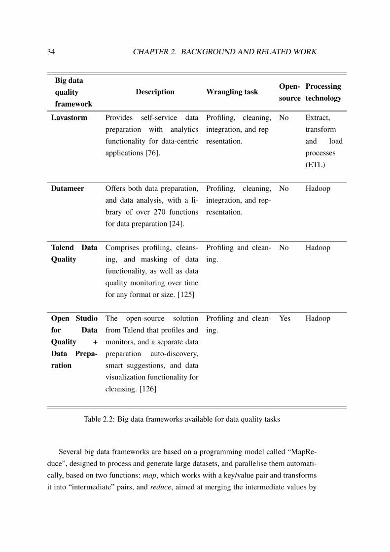
Big dataqualityframework
Description Wrangling taskOpen-source
Processingtechnology
Lavastorm Provides self-service datapreparation with analyticsfunctionality for data-centricapplications [76].
Profiling, cleaning,integration, and rep-resentation.
No Extract,transformand loadprocesses(ETL)
Datameer Offers both data preparation,and data analysis, with a li-brary of over 270 functionsfor data preparation [24].
Profiling, cleaning,integration, and rep-resentation.
No Hadoop
Talend DataQuality
Comprises profiling, cleans-ing, and masking of datafunctionality, as well as dataquality monitoring over timefor any format or size. [125]
Profiling and clean-ing.
No Hadoop
Open Studiofor DataQuality +Data Prepa-ration
The open-source solutionfrom Talend that profiles andmonitors, and a separate datapreparation auto-discovery,smart suggestions, and datavisualization functionality forcleansing. [126]
Profiling and clean-ing.
Yes Hadoop
Table 2.2: Big data frameworks available for data quality tasks
Several big data frameworks are based on a programming model called “MapRe-duce”, designed to process and generate large datasets, and parallelise them automati-cally, based on two functions: map, which works with a key/value pair and transformsit into “intermediate” pairs, and reduce, aimed at merging the intermediate values by

2.3. BIG DATA FRAMEWORKS: TOOLS AND PROJECTS 35
its key [1]. This is the base of the current scale-out approach, being MapReduce themodel that allows the process of big data in commodity hardware [128], and altogetherwith open-source developments, has made the big data frameworks become widelyused among industry and research [128].
Since the release of MapReduce, there have been several projects based on theprogramming model which have been developed, where Hadoop is the name of one ofthe most popular ones. An exhaustive list of all the “big data ecosystem projects” canbe found in an on-going repository available at [92], which includes the names and abrief description of both open-source and proprietary projects. A review on the mostpopular big data frameworks is provided by [49] and [15].
Regarding data wrangling, there are some big data tools available, focused on vi-sualisation and analytics tasks, most of them created towards powering business intel-ligence and being proprietary solutions, however, these frameworks require data to bealready pre-processed. On the other hand, there are few frameworks available for tack-ling data profiling and cleansing tasks; these are described in Table 2.2. The reasonof the apparent lack of frameworks designed specifically for big data quality purposescan be answered by the availability of all the other frameworks, designed as generalpurpose, upon which any kind of application, included those for data wrangling, canbe built and designed, thus, there is an open path to the development of domain spe-cific systems, either based on current frameworks, which could be improved to tackleany specific requirement within the data quality area, or a new framework packed withdefault functions and libraries for big data wrangling. Any selected path requires iden-tification of the wrangling algorithms required, as well as knowledge on how to scalethem to cope with big data.
2.3.1 MapReduce, Hadoop and Spark
MapReduce was presented in 2004 by Google [1], it conforms a paradigm in whichcommodity hardware capacities are leveraged in a hugely distributed architecture [128].One of the attractive components of it was that by using this programming model, de-velopers did not need to be experts on parallel and distributed systems to exploit thepower of the applications coded using MapReduce style. This is because the presentedruntime system solved the details of data partitioning, execution scheduling, failuresand communication across machines, required to utilise resources available in largedistributed systems for big data processing. MapReduce was also presented as a highlyscalable in a scale-out approach, claiming to process data of the order of terabytes (TB)

36 CHAPTER 2. BACKGROUND AND RELATED WORK
on thousands of machines [1].
Communication cost, as mentioned before, is an important issue when handling bigdata; MapReduce model attempts to utilise an optimum network bandwidth by storingdata on the local disks of the machines that conform the cluster, dividing the data into64MB chunks each, and distributing typically 3 copies of them on different machinesacross the cluster, therefore the cluster’s master schedules map tasks closer as possibleto the data that the map function requires [1], or the closest copy of it.
Apache Spark could be simply defined as a “big data Framework”, but its offi-cial definition mentions that it is “a fast and general engine for big data processing,with built-in modules for streaming, SQL, machine learning and graph processing”[46], claimed to be 100 times faster than the “open-source software for reliable, scal-able, distributed computing” [44], Hadoop, another available and widely used big dataFramework that works with the MapReduce programming paradigm. Presumably,Spark achieves better performance by introducing a “distributed memory abstraction”[151]: the resilient distributed datasets (RDDs) that can be used for “lazy evaluations”,caching intermediate results in memory across iterative computations [152, 151]. AnRDD contains five main elements, pieces of a dataset, called partitions; informationabout the parent RDDs or any dependence with another RDD; information on the com-putation needed to create the current RDD, based on its parent partitions; informationabout the most accessible nodes for a given partition of data; and metadata regardingthe RDD scheme [151].
Known as the “Hadoop ecosystem”, there exists several related projects, aimedto be used for big data in different and specific purposes, examples of this platformsinclude Ambari (web based tool for provisioning, managing, and monitoring ApacheHadoop clusters), Avro (data serialization system), Cassandra (resilient scalable multi-master database), Chukwa (data collection system for monitoring large distributed sys-tems), HBase (scalable, distributed database), Hive (data summarisation and ad-hocquerying capabilities), Mahout (scalable machine learning and data mining library),Pig (powerful analysis capabilities with PigLatin, a high-level language), Tez (data-flow programming framework) and Zookeeper (high-performance coordination servicefor distributed applications) [44].
One of the aims of Apache Spark is to have all the possible needs when work-ing with big data, covered with a single solution, so, to achieve this, it allows the useof libraries (SQL and dataFrames, Spark Streaming, MLlib, GraphX, and Third-Party

2.4. SCALABILITY OF DATA MANAGEMENT OPERATORS 37
Packages) and high-level language APIs (Python, Scala, Java and R), adds the capabil-ity to run on Hadoop, Mesos, Standalone, or in the cloud and it is able to access distinctdata sources including HDFS, Cassandra, HBase, S3, Alluxio (known as Tachyon), andany Hadoop data source [46].
2.4 Scalability of Data Management Operators
Previous and related work to this study is scoped to research in which scalability is thekey aspect, from the one addressed using any technique, to extensions of data qualityalgorithms, techniques used specifically with any big data framework, and the relatedwork that is closer to the contribution of this thesis: scalability implemented withApache Spark.
Kale et. al. [69] presented the “NAMD2 program”, a high-performance parallelsimulator of large biomolecular systems behaviour, implemented using C++ and themachine independent parallel programming system coined as Charm++, with an inter-operability framework for parallel processing called Converse. For this program theparallelisation strategy was used to support scalability and a load balancing scheme toincrease performance [69]; this project is still on going as part of the Theoretical andComputational Biophysics research group from the University of Illinois at Urbana-Champaign, currently scaling beyond 500 000 cores for the largest simulations, stillbased o Charm++. Another publication, related to NAMD, recognises the difficultyof coding parallel programs with their used strategy and mentions that the main usageof NAMD is done in “large parallel computers” [106]. These studies then, offer theopportunity to develop a high-performance program that could be both developed withan easier programming strategy and focused on utilisation in commodity hardware,without decreasing its maximum processing capacity.
Before MapReduce, Message Passing Interface (MPI) solutions were the preferredapproach to scalability, as well as parallel and distributed programming and scaling-uptechniques. By the time in which Hadoop emerged, some studies within different areasbegan to explore its usage towards amplifying the capacity of handling large volumesof data, this is the case of a study in which genetic algorithms (GA) were implementedutilising Hadoop and compared against its MPI instances, considering number of vari-ables as volume for the input dataset [143]. Hadoop was then presented as a solutionto the issue of executing genetic algorithms in commodity hardware without failureissues, contrary to what happened with the MPI approach.

38 CHAPTER 2. BACKGROUND AND RELATED WORK
Related to data quality, two studies carried-out experimentations that exploredHadoop’s application for data cleansing processes, the first one, denominated “Bigdata pre-processing data quality (BDPQ) framework” [124], was presented as a set ofmodules to support profiling, selection and adaptation of big datasets. The data cleans-ing module was used to remove noise from electroencephalography (EEG) recordings.The second research mentioned, presented a method for storing and querying medicalResource Description Framework (RDF) datasets using Hadoop to assess for accuracyand validity in medical records [10], removing high costs of data upload, and improv-ing the algorithm’s performance compared to its previous version developed using aJena Java API for RDF approach. This study claims to be the first attempt ever donewith data quality techniques for linked datasets and shows how “utilising data analyticand graph theory techniques can inform a highly optimal query solution” [10]. Futurework related to this study includes testing of the approach on datasets over one billiontriples. Based on the information provided, it is implied that scaling data quality algo-rithms is possible using a big data framework, but more work is required to investigateits full capability with larger datasets and different types of data.
Another algorithm, called PISTON [110], introduces a parallel in-memory spatio-temporal join implemented in a scalable algorithm [110] using load-balancing in amaster/slave model, designed to out perform against existing algorithms with the bestknown performances, where PISTON algorithm addresses recognised characteristicsof long execution time and poor scalability. The model implemented might behavesimilar to the Hadoop-base processing one, however, details on the processing archi-tecture are not provided, limited only to inform details related to the algorithm thatpresents improvements in runtime and capacity to execute joins on spatio-temporaltopological data, achieved due to its inherent behaviour, not because of the infrastruc-ture used, the environment, or the technologies implemented. Masayo Ota et. al. [99]presented in the same year another study of a taxi ride-sharing scalable properties,capable of handling more than 200 million taxi trips information and calculate the op-timum cost-benefit path, this algorithm was tested using Hadoop. However, similarlyto PISTON algorithm’s study, the scalability was presented as obtained mainly becauseof the algorithm structure, not the framework tool.
Sheikh Ikhlaq and Bright Keswani [61] proposed Cloud computing as an alter-native to technologies like Hadoop, but acknowledges that new methods of handlingheterogeneous data without security issues and a good access to information on theCloud are still missing [61]. Even though Cloud computing could bring an option to

2.4. SCALABILITY OF DATA MANAGEMENT OPERATORS 39
avoid investing on local resources, this study does not explain clearly why it considersbig data frameworks as “expensive” to use, when the latter are designed to work notnecessarily with super computers and are part of the available open source platforms.
Another Hadoop’s aided research is presented in the “Highly Scalable Parallel Al-gorithm for Maximally Informative k-Itemset Mining” [115] (PHIKS) study, intro-duced as an algorithm that provides a set of optimisations for itemset mining, tacklingexecution time, communication cost and energy consumption as performance metrics.This novel algorithm was implemented on top of Hadoop using Java as programminglanguage and compared against state-of-the-art itemset mining algorithms on its par-allel form. PHIKS was tested on three different datasets, of 34GB from Amazon Re-views, 49GB from the English Wikipedia articles dataset, and the ClueWeb Englisharticles with 1TB size. In this study, comparisons were made between different algo-rithms and its approaches to the same problem, in all cases using Hadoop as processingengine, however, there is no information regarding the benefits of the framework used,or the parallel techniques implemented compared to a traditional algorithm.
Apache Spark has also been used to support scalability of different algorithms,such as ”Insparq”, an API layer for efficient incremental computation over large datasets designed and implemented on top of Spark using intermediate values for eachcomputation step within an execution, and scoped to be used in analysis of energyconsumption domain with energy data from smart electricity meters [16], where animprovement to the current Spark engine processing was adapted to handle efficientlythat specific kind of data. Another example is shown by Saba Sehrish et. al. [116], whoexecuted an evaluation of Spark’s performance [116] and presented within the HighEnergy Physics (HEP) area with a classification problem algorithm; compared againstan MPI parallel programming instance, the Spark implementation turned out to havelower runtime, mainly because of the level of abstraction that Spark provides to the userregarding certain, and critical decisions, such as task assignment, or distribution anddata location, but Spark still performed better when scaling. This study also providesan example on how specific domain testing is required, by pointing out that, the lackof a “high performance linear algebra library” contributed to the final runtime shownby the Spark instance, therefore, those algorithms requiring that kind of modules, areexpected to look for a more convenient option than Apache Spark.
Regarding the big data frameworks, studies have been made to analyse the perfor-mance of Hadoop and Spark. A scaling-behaviour analysis when using Hadoop andthe MapReduce model [154] was presented identifying three types of applications as

40 CHAPTER 2. BACKGROUND AND RELATED WORK
map-, shuffle- or reduce-intensive, based on the most costly operation required by eachkind of algorithm. The mentioned study provides and analysis on scalability expecta-tions according to the volume of the input dataset, and shows that due to the nature ofthe algorithm, other than relying on the framework or the input size, a linear-scalingis not always present in Hadoop. Other research in which comparisons between Sparkand Hadoop implementations have been evaluated include a “Max-min” scalable antsystem algorithm (MMAS) [144], designed to solve the travelling salesman problemwithin optimisation path algorithms [144], proposing that MMAS could be used to ex-tent neural network, logistic regression or particle swarm algorithms [144], based on itsresults where Spark supported good scalability. Data mining has also been an area inwhich related studies have been developed, showing that dense graph problems can bebenefited by the technique utilised in a single-linkage hierarchical clustering algorithmusing Spark (SHAS) [67], which was evaluated in comparison to an earlier instance ofthe same algorithm in its MapReduce based form [68] with better results shown in thelatest assessment. K-means is also a data mining algorithm evaluated [52] against itsequivalent using Hadoop, showing better execution time when processed with ApacheSpark, and concluding that Spark will become widely used for big data processingtasks, though big data community generally agrees on that Apache Spark is not goingto replace Hadoop, but work together towards merging benefits from both frameworks.
AlgorithmType of
algorithmTechnologyused to scale
Size of thebiggest dataset
Comparedagainst
[69] NAMD
(1999)
Domain Specific:
Molecular
dynamics
A parallel
C++
(Charm++)
36 573
atoms
Sequential
algorithms
simulator
[143] The
ONEMAX GA
(2009)
Domain Specific:
Genetic algorithmsHadoop
100 000
variables
MPI imple-
mentation
[124] BDPQ
(2015)Data quality Hadoop
EEG
recordings
from 22
subjects
Not applicable
[10] Anomaly
detection for
linked data
(2015)
Data quality Hadoop
1024M
triples of
medical
RDF data
Jena imple-
mentation

2.4. SCALABILITY OF DATA MANAGEMENT OPERATORS 41
[16] PHIKS
(2016)Data mining Hadoop 1TB
Parallel imple-
mentation
[16] Insparq
(2016)
Domain Specific:
Incremental energy
analytics
Spark 32GB
Non-
incremental
version
[116]
Classification
algorithm in
HEP (2016)
Data mining Spark 5GBMPI imple-
mentation
[144] MMAS
(2015)
Optimisation
problemsSpark 320 ants
Hadoop
instance
[67] SHAS
(2015)Data mining Spark
2 000 000
data points
Hadoop
instance
[52] K-means
(2015)Data mining Spark
1024MB of
sensor data
Hadoop
instance
Table 2.3: Summary of the most relevant state-of-the-art related studies.
Different ways of leveraging scalability could be found in this literature review,where two identified approaches are shown: scalability based on algorithm design,and scalability based on platform utilised. The first approach comprises design deci-sions, such as heuristics implementation, architectural design (shared-nothing, shared-memory, multi-threaded), complexity, persistence, or general optimisations, whereasplatform scalability comprises choices on the environment utilised regarding the se-lected framework, the programming language and even the cluster size and machinecharacteristics, as well as scaling type (out or up). This research has as main scopeplatform scalability.
Table 2.3 shows a summary of the related studies discussed in this chapter, andreflects that data quality domain is still under development towards scalability, whichrepresents an open area for research where the work presented in this thesis intendsto participate on by expanding data quality query systems. The aim is to explore aplatform approach that could provide those systems the capability to process big data.Chapter 3 presents the designing work carried out towards the mentioned aim, wherea state-of-the-art system’s engine was re-implemented to leverage its big data capabil-ities, preserving the characteristics of its algorithms.

Chapter 3
Designing a Scalable DQ2S
3.1 The Data Quality Query System (DQ2S)
The Data Quality Query System (DQ2S) is a framework and tool that allows measuringsome of the quality dimensions (completeness, timeliness, accuracy, and reputation)from a given data by profiling it [26]. This system reads data from a storage location,and performs database algebra operations to profile the quality of the data according tothe queries applied, allowing users to get the data quality information in the same waythey query if it was done using SQL commands. The DQ2S is in fact an interface tostorage and an extension of the SQL query engine that can be implemented to utilise ei-ther a relational database or a storage file system. DQ2S provides functionality withoutrequiring users to be aware of the stored quality-related information or the data pro-filing algorithms implemented at the physical level. This framework can be used withtraditional data management techniques, however, the DQ2S original implementationdoes not exploit parallelism and cannot cope with very large datasets [26].
This research covers the design, implementation and evaluation of some of thealgorithms included in the DQ2S towards increasing the data volume limit that canbe handled by the DQ2S, considering speed of processing, scalability and resourcerequirements. For the mentioned purpose, a big data framework was selected in orderto explore the features that could be obtained for DQ2S, and seeking for performanceimprovements such as memory required, processing capacity and resource utilisationcompared to its usage without the framework. The focus of this research is targeted atproviding scalable, cost-effective, highly-automated, and optimised solutions.
42

3.1. THE DATA QUALITY QUERY SYSTEM (DQ2S) 43
3.1.1 The Framework
The DQ2S is a useful contribution to the data management area, where informationsystems, analytical tasks based on data, and more recently, big data and business intel-ligence require data quality awareness, as discussed in Section 1.1. DQ2S is a novelcontribution to the data quality area, as exposed on its original publication at [26],where the related work discussion reflects DQ2S is flexible, by allowing users to setthe configuration required but without being too broad to be highly complex [26], sup-porting optimisation and enabling ease of use when operated by users already familiarwith SQL.
DQ2S appears as a complementary functionality to the data quality process withindata management by facilitating a quality-profile of the data in use, leading to supportthe cleansing tasks within the data wrangling effort, as well as handling informationto allow users to know their data, which is designed as one of the challenges whenconsidering big data quality needs, and because a data profile provides a step towardsa high level of confidence of the data’s fit to conduct analytical tasks [26], all of theabove makes DQ2S a viable tool within information systems aimed at data quality,however, the system requires further research and experimentation to develop a DQ2Scapable of handling efficiently larger volumes of data. Such experimentation couldprovide a baseline towards scaling other data quality management approaches.
The basic DQ2S work [26] shows experimental results of the queries with two dataquality dimensions tested, timeliness and completeness, where the quickest runtimeobtained on an average of three runs, was around 15 minutes for a dataset of 100 000rows, and the slowest time was an average of 76 minutes for the same dataset. An im-portant note on the mentioned results is that two versions of the queries were executed,where one was an optimised version with an implementation of heuristics for query ex-ecutions in relational databases, which reduced 29% the execution time for the Timeli-ness query, and 67% for the completeness query; this reduction was achieved due to adecrease on the intermediate resources size, hence, the processing of the datasets wasless intense and the memory requirement was smaller, thus, paging that happened inthe process was also reduced [26], this incurred on diminishing I/O costs, nevertheless,even with the optimised versions, 15 minutes were required to handle 100 000 rows,and an increasing of 70.6 times the runtime obtained from 10 000 to 100 000 rows onthe best of the cases (Timeliness query with optimisation) suggest the original DQ2Simplementation is not adequate to handle larger datasets. The limitation appears on

44 CHAPTER 3. DESIGNING A SCALABLE DQ2S
the memory requirements, where the queries were optimised on its process, but mem-ory handling and I/O processes are still the same for both versions (with and withoutheuristics), and that is not inherent to the algorithm but to the architectural environ-ment in which the processing is carried out, this appears as an opportunity for big dataframeworks, specialised on big data processing optimisation with regards to architec-ture models that allow machines to handle larger data than its actual memory space,discussion on big data framework approaches and details is presented in Section 2.3.
This research aims at exploring a popular and rising big data framework based onthe MapReduce paradigm, towards an analysis of its suitability to extend the DQ2Sfor big data. Apache Spark supports in-memory processing, which reduces I/O costs,and provides a data structure that facilitates usage of intermediate results in memory,offering options to tune the data partitioning, and supporting a rich set of operations tomanipulate the data, as well as resilient behaviour [152].
3.1.2 The Query
DQ2S supports the implementation of four quality dimensions applied on relationalmodels. The dimensions include accuracy, completeness, timeliness, and reputation,which are applicable in several domains concerned to e-Business, e-Science and In-formation Systems, specially when dealing with geographical data [26]. Within ane-Business context, completeness and timeliness were the dimensions utilised on theevaluation of DQ2S, since the queries implemented covered several important use casesin the domain [26]. The Timeliness query is an appropriate dimension to target for im-provement to the objectives of this study, since the results of the DQ2S work [26]indicated that Timeliness queries produced the slower runtimes, and furthermore, theTimeliness query includes only one profiling operator and one join, simplifying thetasks of isolating the properties of the algorithm to enable experimentation with bigdata frameworks, whereas the completeness algorithm is composed of two profilingoperators and two joins. A single factor analysis provides accuracy on quantifying theresults, and the higher runtime offers a wider opportunity for optimisation, consideringthat, if a big data framework can provide support to the most expensive query, it mighteasily support less intensive queries.
Timeliness is part of the Contextual Data Quality (CDQ) category [155], where thedegree of quality depends on the context of the data’s purpose, for example, some datamight be timely enough to support data driven decisions utilising weekly reports onthe data, where its timeliness quality would be lesser if pretended to be used for the

3.1. THE DATA QUALITY QUERY SYSTEM (DQ2S) 45
following weekly report, however, if the same data is taken on a semester based task,its timeliness degree posses a different value. Timeliness could be defined as the extentto which the data is not outdated to be useless for its intended use.
The timeliness data quality dimension, was modelled as a query for DQ2S imple-menting formulas to calculate the timeliness degree [26], based on timeliness calcula-tion defined for information products [8], but applicable within a general scope for IS,as follows:
Timeliness(v,s) = max[(1− Currency(v)Volatility(v)
),0]s
(3.1)
Where v represents a unit of data, and s represents a control value to the sensitivityof the currency-volatility ratio, its increase or decrease will be done depending on howmuch impact the volatility produces, for example, if volatility is high, and thus withinthe given context, the timeliness is highly affected, s should increase from 0.5 (almostno impact) to a value of 2. Both v and s are given to the calculation as input, whereascurrency and volatility are computed with the correspondent formulas shown in 3.2,and 3.3 equations. Currency is the age of the data given by the time data was keptstored and the age it had when it was first saved, and volatility shows a measure oftime upon which data is not outdated.
Currency(v) = DeliveryTime(v)−LastU pdateTime(v)+Age(v) (3.2)
Volatility(v) = ExpiryTime(v)−LastU pdateTime(v)+Age(v) (3.3)
Timeliness calculation is given on a 0 - 1 scale, where the scale can be seen as 0to 100% of timeliness degree. The Timeliness query specified for the study requires toselect, from an e-Business dataset, the orders that are pending and have been waitingto be validated for more than 50% of the total waiting time. Figure 3.1 shows the queryexpressed using the query language defined for DQ2S (called DQ2L), and Figure 3.2shows the same query expressed with SQL, which show one of the useful aspects ofDQ2S when querying on a SQL style, as well as the insight of the general algorithmprocess required by the query; both queries retrieve the same output. The output to theTimeliness query needs to show the order no and the timeliness score of those pendingorders that turn out to have a timeliness score lower than 0.5.

46 CHAPTER 3. DESIGNING A SCALABLE DQ2S
Figure 3.1: Timeliness query expressed with DQ2L [26].
Figure 3.2: Timeliness query expressed with SQL [26].
3.1.3 The Datasets
Figure 3.3: OrderT dataset’s first 9 rows.
Figure 3.4: StatusTimelinessQR dataset’s first 9 rows.
The e-Business data utilised for querying with DQ2S has five relations, each onewith different information and scheme. The datasets are:
• orderT: Contains information about the orders made to the e-Business.
• part: Is the inventory of the parts the e-Business sells.
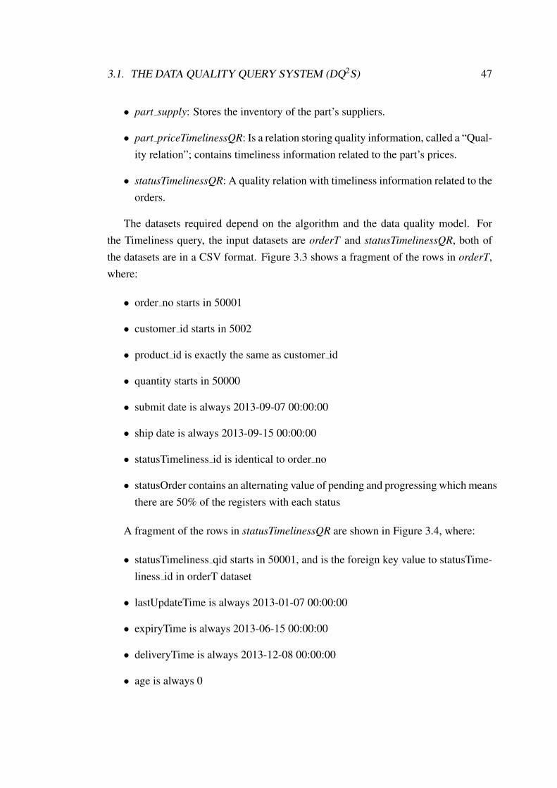
3.1. THE DATA QUALITY QUERY SYSTEM (DQ2S) 47
• part supply: Stores the inventory of the part’s suppliers.
• part priceTimelinessQR: Is a relation storing quality information, called a “Qual-ity relation”; contains timeliness information related to the part’s prices.
• statusTimelinessQR: A quality relation with timeliness information related to theorders.
The datasets required depend on the algorithm and the data quality model. Forthe Timeliness query, the input datasets are orderT and statusTimelinessQR, both ofthe datasets are in a CSV format. Figure 3.3 shows a fragment of the rows in orderT,where:
• order no starts in 50001
• customer id starts in 5002
• product id is exactly the same as customer id
• quantity starts in 50000
• submit date is always 2013-09-07 00:00:00
• ship date is always 2013-09-15 00:00:00
• statusTimeliness id is identical to order no
• statusOrder contains an alternating value of pending and progressing which meansthere are 50% of the registers with each status
A fragment of the rows in statusTimelinessQR are shown in Figure 3.4, where:
• statusTimeliness qid starts in 50001, and is the foreign key value to statusTime-liness id in orderT dataset
• lastUpdateTime is always 2013-01-07 00:00:00
• expiryTime is always 2013-06-15 00:00:00
• deliveryTime is always 2013-12-08 00:00:00
• age is always 0
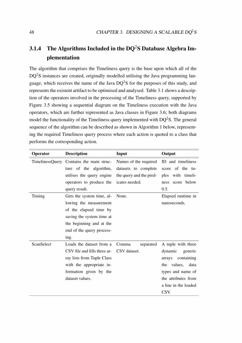
48 CHAPTER 3. DESIGNING A SCALABLE DQ2S
3.1.4 The Algorithms Included in the DQ2S Database Algebra Im-plementation
The algorithm that comprises the Timeliness query is the base upon which all of theDQ2S instances are created, originally modelled utilising the Java programming lan-guage, which receives the name of the Java DQ2S for the purposes of this study, andrepresents the existent artifact to be optimised and analysed. Table 3.1 shows a descrip-tion of the operators involved in the processing of the Timeliness query, supported byFigure 3.5 showing a sequential diagram on the Timeliness execution with the Javaoperators, which are further represented as Java classes in Figure 3.6; both diagramsmodel the functionality of the Timeliness query implemented with DQ2S. The generalsequence of the algorithm can be described as shown in Algorithm 1 below, represent-ing the required Timeliness query process where each action is quoted to a class thatperforms the corresponding action.
Operator Description Input Output
TimelinessQuery Contains the main struc-
ture of the algorithm,
utilises the query engine
operators to produce the
query result.
Names of the required
datasets to complete
the query and the pred-
icates needed.
ID and timeliness
score of the tu-
ples with timeli-
ness score below
0.5.
Timing Gets the system time, al-
lowing the measurement
of the elapsed time by
saving the system time at
the beginning and at the
end of the query process-
ing.
None. Elapsed runtime in
nanoseconds.
ScanSelect Loads the dataset from a
CSV file and fills three ar-
ray lists from Tuple Class
with the appropriate in-
formation given by the
dataset values.
Comma separated
CSV dataset.
A tuple with three
dynamic generic
arrays containing
the values, data
types and name of
the attributes from
a line in the loaded
CSV.

3.1. THE DATA QUALITY QUERY SYSTEM (DQ2S) 49
Tuple Creates a data structure
containing the data in-
gested by ScanSelect
and schema information
(data types and attribute
names).
Two dynamic generic
arrays, one containing
the data types names
and the second array
formed by the attribute
names.
A data structure
formed by three
dynamic generic
arrays (data values,
data types, and
attribute names).
Predicate Evaluates a given predi-
cate and returns a boolean
value depending on its
compliment or not, ac-
cording to the operator
and the evaluated values
within it.
A predicate made of
two operands and one
comparison operator.
Boolean value
telling if the pred-
icate was true or
false after applied
on a given data.
Join Joins two dynamic
generic arrays based on a
given join predicate.
Two dynamic generic
arrays and a join pred-
icate specifying the
joining statement to
determine which rows
need to be joined.
A single dynamic
generic array with
joined data.
JoinPredicate Is a support algorithm to
the Join operator. Evalu-
ates the predicate against
the dynamic generic array
and retrieves a Boolean
value on the predicate
correspondence with the
data.
Join predicate. Boolean value
telling if the join
predicate was
true or false after
applied on a given
data.
Timeliness Calculates the timeliness
score based on the formu-
las presented in Section
3.1.2 of this chapter.
A dynamic generic ar-
ray containing the data
required to calculate
the score.
The dynamic
generic array
utilised as input
plus a new column
with the correspon-
dent calculated
timeliness score.

50 CHAPTER 3. DESIGNING A SCALABLE DQ2S
Select Filters a dynamic generic
array and creates a new
one based on the result
obtained from the Predi-
cate class.
Filter predicate and a
dynamic generic array
to apply the filter on.
A dynamic generic
array containing
the filtered data.
Project Extracts columns from
a dynamic generic array
based on a list of at-
tributes given (name of
the columns).
List of attributes and a
dynamic generic array.
A dynamic generic
array containing
the data that cor-
responds to the
required columns.
Table 3.1: Operators comprising the DQ2S Timeliness query.

3.1. THE DATA QUALITY QUERY SYSTEM (DQ2S) 51
Figu
re3.
5:G
ener
alse
quen
cedi
agra
mfo
rthe
Tim
elin
ess
quer
y,bu
ildfr
omth
eJa
vaD
Q2 S
inst
ance
.

52 CHAPTER 3. DESIGNING A SCALABLE DQ2S
Figure 3.6: Class diagram for the Java DQ2S engine.

3.1. THE DATA QUALITY QUERY SYSTEM (DQ2S) 53
Algorithm 1. Part 1 - TimelinessQuery Class.1: function MAIN( )2: Get the current system time . Timing class
Start Create first array . Selects all the orders from orderT dataset with “pending” status
and saves them in a dynamic array
3: Get the name of the input dataset← “orderT”4: Form the predicate to extract orders with “pending” as status . Predicate class
5: From the dataset with the given name, save the data and its schema on adynamic generic array applying the given predicate selection
. ScanSelect class
EndStart Create second array . Selects all the registers from “statusTimelinessQR” dataset and
saves them in a dynamic array
6: Get the name of the input dataset← “statusTimelinessQR”7: Create a null predicate . Predicate class
8: From the dataset with the given name, save the data and its schema on adynamic generic array applying the predicate selection
. ScanSelect class
. Tuple class
EndStart Create a Join . Joins the information in the first and the second array on a given join
predicate as the joining point, and saves the content in a new array
9: Create a join predicate to join the arrays on “orderT.statusTimeliness id” and“statusTimelinessQR.statusTimeliness qid” . JoinPredicate class
10: Specify which two arrays should be joined11: Join two given arrays on the given predicate and generate a new array with the
joined data . Join class
End

54 CHAPTER 3. DESIGNING A SCALABLE DQ2S
Algorithm 1. Part 2 - TimelinessQuery Class.Start Create a Timeliness. Calculates the timeliness score with the information in the joined array. Copies the content of
the joined array plus a new attribute with the corresponding scores.
12: Set the name for the column to add← “timeliness”13: Specify the array to utilise for the Timeliness score calculation14: Calculate the Timeliness score from the information within the given array,
and add the score to a column with the given name . Timeliness class
EndStart Create a Select
. Selects the information of the tuples which timeliness score is < 0.5 from the latest
array created
15: Form the predicate to extract orders with timeliness score below 0.5. Predicate class
16: Generate a new array applying the given predicate to the latest array formed. Select class
EndStart Create a Project
. Extracts the column with the Id and the column with the timeliness score from
the latest array, and saves only the content of those attributes as the final result of the query.
17: Get the attributes name to extract from the latest array created ←“statusTimelinessQR.statusTimeliness qid”, “timeliness.score”
18: Specify the array to utilise and the attributes to get . Project class
19: Create the final array only with the columns required . Project class
End20: Print Final array21: Get the current system time . Timing class
22: Calculate the elapsed time since the beginning of the processing . Timing class
23: Print Elapsed time calculated24: end function

3.2. THE ARTIFACT 55
3.2 The Artifact
The artifact of this study is composed by the DQ2S instances, which will comprisean added artifact to the existent one, the Java version. Java is a general purpose pro-gramming language, which provides an opportunity to explore DQ2S performance andscalability with big data programming languages, presumably optimised to cope withlarge volume of data, hence, the algorithm was developed utilising different technolo-gies, including a big data framework to provide answers to the research questions pre-sented in Section 4.1, and support to the hypothesis validation presented in the samesection. The source code of the DQ2S developed instances, and the original Java codeis shown in Appendix A, this section presents details on the instances development andinternal composition.
3.2.1 The Java DQ2S
Table 3.2 shows details on the technical aspects of components that comprise the JavaDQ2S, as well as information on key pieces of code utilised to develop the instance,which are important for the understanding of the technical behaviour, as this is thebase for extending the algorithm to be developed for its usage with other big datatechnologies. Some operators did not require any special or outstanding codificationthan common and basic pieces of code ( e.g. if statements or method calls).
Operator Technical Description Key piece of code
TimelinessQuery Contains the main method. Creates the
required objects utilising the classes
involved in the timeliness query, and
calls for the execution of the methods
from the external classes through the
created objects.
None.

56 CHAPTER 3. DESIGNING A SCALABLE DQ2S
Timing Contains three methods: StartTime,
stopTime, and durationTime.
StartTime gets the system time of the
moment in which is called, and saves
it in a variable; the second method has
the same functionality as StartTime,
but is required to store the system time
in a second moment; the third time
calculates the arithmetic difference
between the two variables created, and
prints the value in nanoseconds. This
is the elapsed time from the processing
that happened between the first system
time and the second.
System.nanoTime() is used to
get the current value of the sys-
tem timer in nanoseconds.
ScanSelect Gets as parameter the name of the
dataset to load, loads it with a buffered
reader, which allows a line per line
reading. Line per line is saved into
a dynamic generic array created under
the custom Tuple data structure.
BufferedReader rs =
new BufferedReader(new
FileReader(csvFile)) to
read the CSV file from storage to
the buffer, then rs.readLine()
is used to read line by line
from the correspondent buffer
containing the data.
Tuple Creates a data type containing three ar-
ray lists: one for the data values, filled
in the ScanSelect class; one for the
data types; and a third one for the at-
tribute’s names (columns), which are
filled within this class with a for state-
ment.
ArrayList<Object>() to
save the data, and Add() to add
values to the array within the
for statement.
Predicate Gets a predicate formed by one first
operand, an operator, and a second
operand, then evaluates both operands
with the operator according to the op-
erator’s data type, and returns true
or false as the evaluation result indi-
cates.
None.

3.2. THE ARTIFACT 57
Join Copies the data from two Tuple ob-
jects into a new one, integrating the
data from both input objects. Once the
new Tuple object exists, an array list is
generated with the data from that new
Tuple. These data is only the content
that matches the given join predicate,
this is, only the rows that get a true
value from JoinPredicate.
Utilises addAll() inside a for
statement to copy all the data
from the Tuple objects in-
dicated, and add() to copy
only the rows with a true
boolean value obtained from the
JoinPredicate class.
JoinPredicate Gets the position in which required
operands are in a Tuple, to obtain the
correspondent data type, then accord-
ing to the data type, the class evalu-
ates if the operands conform a true or
false comparison with the given oper-
ator. Returns the evaluation result in
boolean.
None.
Timeliness From the input Tuple, extracts the
quality information required to calcu-
late the currency, volatility and time-
liness. With the data extracted calcu-
lates the timeliness score based on the
formulas 3.1, 3.2, and 3.3 presented in
this chapter, then adds a new column to
the original Tuple, with the timeliness
score calculated for each row.
Utilises addAll() inside a for
statement to copy all the data
from the input Tuple in a new
one, then adds to the new Tuple
the timeliness score per row with
add(). get Time() was used
to get the time in miliseconds in
unix time, aslo known as epoch
time.
Select Utilises a Predicate object from the
Predicate class, and a Tuple object.
Whenever the Predicate class returns a
true value, this class adds the evaluated
Tuple to a new one.
Utilises add() inside a for
statement to copy into a new
Tuple the correspondant rows,
as many times as true values are
obtained from the Predicate
class.

58 CHAPTER 3. DESIGNING A SCALABLE DQ2S
Project Gets a list of column names and an ar-
ray list with data values, then copies the
data from the columns indicated into a
new array list, which is later converted
to Tuple object.
Utilises add() inside a for
statement to copy into a new
Tuple the rows from the given
columns.
Table 3.2: Java DQ2S technical description
3.2.2 The Python DQ2S Implementation
Scala, R, and Python are considered programming languages suitable for big data ana-lytics. These contain classes specially designed to support data analysis tasks, such asprofiling and mining large datasets [31, 87], there are other programming languages ofthis kind, such as Julia or Go, but those are less popular than Scala, R or Python.[31, 14]. For scientific applications, and use within enterprises and organisations,Python is on the top 10 most popular worldwide, whereas Scala is known better forweb and mobile development, and still less popular than Python in those situations[32]. R is gaining popularity, getting closer to Python and gradually replacing C# forgeneral usage [14], but around 458,000 public repositories for Python [31], makes ita clear winner in the data science landscape. Due to its growing popularity, Pythonwas selected as the approach to test scalability and performance for DQ2S instead ofother “big data languages”. Table 3.3 presents the main differences implemented fromre-engineering the Java DQ2S into a Python instance, where the third columns showspieces of code that are significantly different to the same functionality utilised in Java.The general development was done by utilising the equivalent Python code, whichmost of the time was only a syntax change (to Python proper syntax).

3.2. THE ARTIFACT 59
Operator Main differences with Java instance Key piece of code
TimelinessQuery Contains the main method that cov-
ers the same functionality as the Java
DQ2S. The only difference is that the
final printing requires a time consum-
ing for statement to print line by line,
however, the experiments for this study
does not calculate the time considering
the final printings too, but only the gen-
eral processing time of the query.
None.
Timing Utilises a different approach to get the
system time in nanoseconds.
int(round(time.time()*
1e9)) is used to get the current
value of the system timer in
nanoseconds.
ScanSelect To load the CSV content, a Python
CSV reader was utilised, and the equiv-
alent method to copy rows into an ar-
ray.
import csv was used to utilise
csv.reader(csvFile), a
reader for tabular data in CSV
format, and array.append()
was used as equivalent to the
Java method add().
Tuple, Select &
Project
The equivalent method to copy rows
into an array.
array.append() was used as
equivalent to the Java method
add().
Predicate &
JoinPredicate
None. None.
Join The equivalent method to copy rows
into an array.
array.append() was used as
equivalent to the Java method
add(), and array.extend()
was used as equivalent to the
Java method addAll(). The
high level difference between
append and extend is that extend
can add more than one item each
time.

60 CHAPTER 3. DESIGNING A SCALABLE DQ2S
Timeliness Required a custom function to convert
the Timestamp values into miliseconds
epoch time.
utcfromtimestamp(),
strptime(), and total
seconds() * 1000.0 was
utilised instead of the Java
method get Time().
Table 3.3: Python DQ2S technical description
3.2.3 The Optimised Python DQ2S Implementation
Python Pandas library (from panel data, “a common term for multidimensional datasets encountered in statistics and econometrics” [87]) appeared as a solution to Pythonlack of statistics and data analysis capabilities, where R, MatLab, Stata and SAS weredominating the area [87]. Python Pandas as a scientific library provide data struc-tures and methods with focus on structured data utilisation, with optimised and robustsolutions to manipulate those kind of data, which is a strong quality with high expec-tation for the DQ2S algorithm. Pandas provides a data structure called “dataFrames”,inspired by R [87], which supports SQL like manipulation. The Optimised PythonDQ2S is called “Optimised” in relation to the Pandas library which is the main com-ponent utilised for this DQ2S instance. Table 3.4 presents a description of the changesrequired for the re-engineering of DQ2S to its version with an optimised library, whereeven the lines of code were significantly reduced due to the concise functionality Pan-das library provide.
Operator Main differences with Python instance Key piece of code
TimelinessQuery When utilising the Pandas library and
dataFrames to store the data instead
of array lists, the final printing can be
done with a Pandas defined method
to print dataFrames content. The rest
of the codification is exactly the same
within the TimelinessQuery class.
dataFrame.head(n).
to string() is utilised to print
the content of the dataFrame
containing the results, where n
is the number of rows to print.
This method is equivalent to
printing the final results from
the correspondent Tuple object
in the Java and Python instances.
Timing None. None.
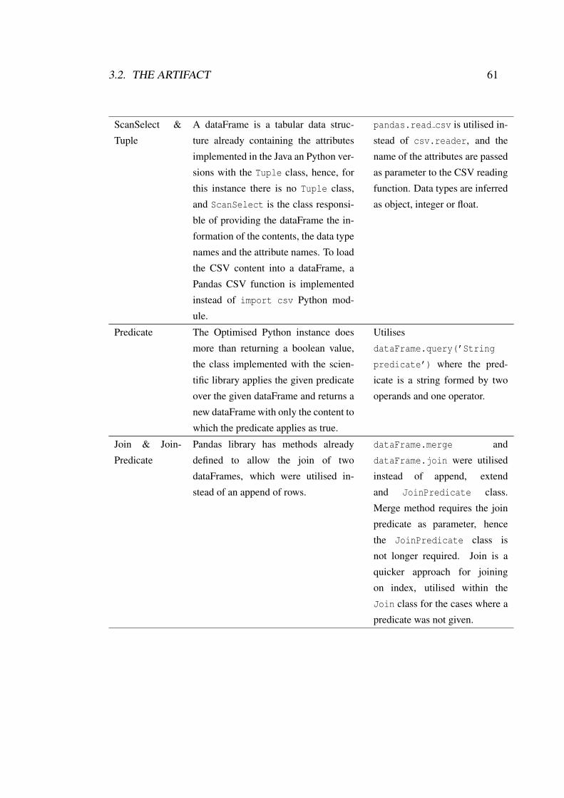
3.2. THE ARTIFACT 61
ScanSelect &
Tuple
A dataFrame is a tabular data struc-
ture already containing the attributes
implemented in the Java an Python ver-
sions with the Tuple class, hence, for
this instance there is no Tuple class,
and ScanSelect is the class responsi-
ble of providing the dataFrame the in-
formation of the contents, the data type
names and the attribute names. To load
the CSV content into a dataFrame, a
Pandas CSV function is implemented
instead of import csv Python mod-
ule.
pandas.read csv is utilised in-
stead of csv.reader, and the
name of the attributes are passed
as parameter to the CSV reading
function. Data types are inferred
as object, integer or float.
Predicate The Optimised Python instance does
more than returning a boolean value,
the class implemented with the scien-
tific library applies the given predicate
over the given dataFrame and returns a
new dataFrame with only the content to
which the predicate applies as true.
Utilises
dataFrame.query(’String
predicate’) where the pred-
icate is a string formed by two
operands and one operator.
Join & Join-
Predicate
Pandas library has methods already
defined to allow the join of two
dataFrames, which were utilised in-
stead of an append of rows.
dataFrame.merge and
dataFrame.join were utilised
instead of append, extend
and JoinPredicate class.
Merge method requires the join
predicate as parameter, hence
the JoinPredicate class is
not longer required. Join is a
quicker approach for joining
on index, utilised within the
Join class for the cases where a
predicate was not given.
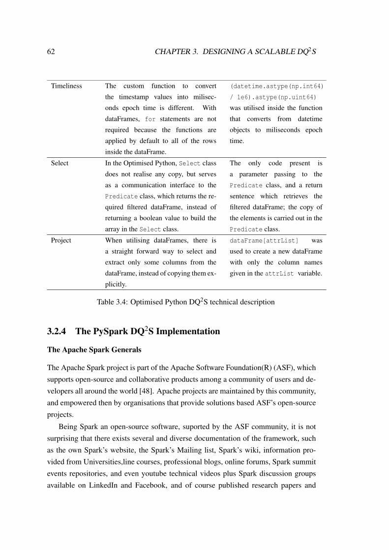
62 CHAPTER 3. DESIGNING A SCALABLE DQ2S
Timeliness The custom function to convert
the timestamp values into milisec-
onds epoch time is different. With
dataFrames, for statements are not
required because the functions are
applied by default to all of the rows
inside the dataFrame.
(datetime.astype(np.int64)
/ 1e6).astype(np.uint64)
was utilised inside the function
that converts from datetime
objects to miliseconds epoch
time.
Select In the Optimised Python, Select class
does not realise any copy, but serves
as a communication interface to the
Predicate class, which returns the re-
quired filtered dataFrame, instead of
returning a boolean value to build the
array in the Select class.
The only code present is
a parameter passing to the
Predicate class, and a return
sentence which retrieves the
filtered dataFrame; the copy of
the elements is carried out in the
Predicate class.
Project When utilising dataFrames, there is
a straight forward way to select and
extract only some columns from the
dataFrame, instead of copying them ex-
plicitly.
dataFrame[attrList] was
used to create a new dataFrame
with only the column names
given in the attrList variable.
Table 3.4: Optimised Python DQ2S technical description
3.2.4 The PySpark DQ2S Implementation
The Apache Spark Generals
The Apache Spark project is part of the Apache Software Foundation(R) (ASF), whichsupports open-source and collaborative products among a community of users and de-velopers all around the world [48]. Apache projects are maintained by this community,and empowered then by organisations that provide solutions based ASF’s open-sourceprojects.
Being Spark an open-source software, suported by the ASF community, it is notsurprising that there exists several and diverse documentation of the framework, suchas the own Spark’s website, the Spark’s Mailing list, Spark’s wiki, information pro-vided from Universities,line courses, professional blogs, online forums, Spark summitevents repositories, and even youtube technical videos plus Spark discussion groupsavailable on LinkedIn and Facebook, and of course published research papers and

3.2. THE ARTIFACT 63
books. Having all of those sources available, this study does not intend to be part ofanother source of Spark’s information, however, it might be valuable to clarify somebasic concepts that were found rather ambiguous among all of the diversity of sources.
Spark itself is written on Scala language, which runs on the Java Virtual Machine(JVM) [18]. All of Spark’s general functionality relies on the usage of the Java VirtualMachine, taking advantage of the JVM’s memory management and garbage collection(GC) [97] that this platform-independent environment provides. The usage of JVMalso preserves the possibility for Spark’s integration with other projects of the Hadoopecosystem (refer to Section 2.3.1 for details of Hadoop ecosystem), which are JVMbased. Each JVM has its own memory allocation, its own GC process, and its ownthreads that access its own memory area. Spark’s architecture comprises basically fiveconcepts upon which all of its computations are developed in a cluster, described be-low. Table B.1 in Appendix B shows the configuration defaults of each of the conceptsdescribed, and table B.2 in the same appendix shows the parameters that can be usedto modify the default values within a Spark Standalone cluster.
1. Driver.
Driver process. Also known as the driver program, this process runs on itsown JVM with 1 core and 1GB by default. The following are the activities thatthe driver is in charge of performing:
• Process the main() function of the application.
• Create the SparkContext object, which tells the driver how and where toaccess the master node.
• Connect and communicate with the cluster manager process to know thecluster resource’s availability.
• Split an application into tasks.
• Schedule the tasks on the available executors.
• Send the application code to the executors.
Driver node. This is the node on which the driver process is running. Itcould be a node outside the Spark cluster (client mode), or a node inside thecluster (cluster mode).
2. Cluster Manager.

64 CHAPTER 3. DESIGNING A SCALABLE DQ2S
Master process. The cluster manager can also be called the master process.This process schedules the allocation of Workers and its executors within thecluster. The cluster manager can take the form of Spark’s Standalone (Spark’sown resource manager), YARN (Hadoop’s resource manager) or Mesos (a gen-eral resource and scheduling manager for clusters).
The Standalone cluster manager performs the following activities:
• Allocates resources to the worker nodes.
• Utilises the worker to create executors for the driver.
• Communicates its workers and executors availability to the driver processonce the driver connects to it.
YARN and Mesos cluster managers in general perform the same activities, how-ever, could be more involved than the Standalone manager when schedulingtasks.
Master node.The master node is the machine within the cluster in which themaster process is running.
3. Worker.
Worker process. Also known as the Slaves process, this is also createdon its own JVM. A worker is in charge of reporting to the master process itsresource availability, so the master can deliver that information to the driver.
There are two important things to note about the configuration of the Workers:
• When setting number of Workers, memory per worker and cores per worker,the cluster will allocate the specified per node on the cluster, not per thewhole cluster.
• The cores and memory allocated to each worker, is only to indicate theworkers the resources each worker can give out to its executors, not theactual resources that the worker is going to use. The worker by default runsusing 1G and 1 core, which is enough for the majority of Spark applicationsbecause of the activities it performs.
Worker node. A worker node is a machine within the cluster that containsone or more worker processes.

3.2. THE ARTIFACT 65
4. Executor. An executor is the JVM process on a worker node that processes thetasks that constitute the application. There are some noticeable aspects of anexecutor:
• By default one executor is created per worker process, taking all the avail-able cores that the worker has to give out and 1GB of memory, however thissetting can be changed to either have more than one executor per workerprocess and/or allocate more memory for the executor’s JVM.
• The executor process is the one that loads into its memory the data fromstorage, processes the computations and produces the results.
• Each executor loads into memory only the required data for its allocatedtask.
• An executor process will not start if there is not enough resources allocatedby the worker, for example, if it is required 2 executors, each one with10GB of memory but the worker has allocated 12GB, only 1 worker willstart.
• Each executor computes tasks in multiple threads.
5. Cores. Spark cores in reality are not CPU cores but threads; when number ofcores is set, this number means how many tasks should be handled simultane-ously by the executor. This is the reason of why setting a larger number for the“cores” than the available CPU cores of the machine, will not trigger any errorwhen starting a Spark cluster and submitting an application. The best practice,however, is to adhere its usage to a value equal to the number of CPU cores onthe worker node.
Having more threads processed simultaneously could cause an overhead becauseof scheduling and communication time, resulting in more time spent on overheadcomputation than in the actual processing of the tasks.
For this study, from now on, when referring to cores it is done to the defini-tion described above: the number of tasks handled at the same time by anexecutor. When referring to CPU cores, it will be done explicitly.
Spark’s elements relate to each during the processing of an application, followingSpark’s cluster general operation:

66 CHAPTER 3. DESIGNING A SCALABLE DQ2S
1. The cluster manager (also known as the master process) has to be up before anyapplication is submitted.
2. Once submitted and the SparkContext created, the driver program starts and asksthe master for resources.
3. The worker communicates its resource availability to the master.
4. The master uses the worker to create executors. It decides where to launch themaccording to the resources availability reported by the workers.
5. The driver allocates tasks to the executors to process.
6. The executors can communicate only between executors of the same application.
7. Once all the tasks have been finished, results are sent back to the driver.
8. The driver then stops the SparkContext, all executor processes also stop andthe cluster’s resources are released. The workers and master processes are notstopped when the driver stops.
Apache Spark as a framework for big data processing provides the following ben-efits [46, 151, 152]:
• Provides in-memory processing by loading data from storage to its JVM execu-tor’s memory, allowing these to work with the data without investing too muchtime on storage I/O.
• Its data structures, Resilient Distributed Dataset (RDD) and dataFrames, parti-tions the data so it can be processed in parallel, adds information that enables torecompute a partition in case of failure, and provides Spark the ability to processlarge volumes of data by allowing the executors to load only the partition that itrequires according to the task that was given to that executor.
• Provides fault tolerance and “speculative” processing by relocating tasks whena failure occurs or when the processing is being slow.
• Supports high level programming, with Python, Scala, Java and R ApplicationProgramming Interfaces (APIs), which gives flexibility and ease of use for awider range of users without trading much on processing speed inherent to thelanguage. All of the different languages run at JVM speed on Spark. Spark

3.2. THE ARTIFACT 67
implements sockets that allow each language to call Java Methods. A widerdescription on how the API implemented on this study (Python API - PySpark)is used internally with Spark can be found in the next subsection of this chapter.
• Offers built-in libraries that gives Spark its multi-purpose characteristic: SQLwith a Query Optimiser, Machine Learning libraries (MLib), Streaming supportand Graph computation. All of them are used on top of the Spark Core Engine.
• Supports integration with all of the major Hadoop projects, included Hadoop’sdistributed file-system and Hadoop Resource Manager, which supports Spark tocomplement itself with other’s programs capacities and allows Spark to be anoption for users that are familiar with Hadoop and its related projects (refer toSection 2.3.1).
Spark Python API
The applications developed with the Python API are called “PySpark” applications.Python API was built on top of the Java API which is on top of the Spark Core Enginewritten in Scala, this structure allows Python to be utilised with a Spark that internallyworks with JVMs. When a PySpark application is submitted, the process is the same asdescribed earlier in this section, but there some specific details that are present with thePython API. The process of Apache Spark with Python API starts on the driver node,then PySpark utilises py4j socket to enable Python programs running in the pythoninterpreter to utilise Java methods as if there were the same programming language.This is how from the Python programme, a Spark context JVM is launched. Then,the executor process launches a Python process (daemon.py) with as many child pro-cesses as cores were set in the Spark parameters. Next, there is a custom pipe writtenby the Spark engineers, capable of moving high volumes of data at high velocity be-tween the daemon.py and the executor’s JVM. The data is loaded to the daemon.pyfrom the JVM, but functions are serialised in the called “pickles objects” (serialiseddata structures of size up to 1MB each “pickle”) from the driver process, and sentto the daemon.py process, this last location is where the functions are “unpickled”(unserialised). Each child process carries out the function to its given data, howeverSpark’s library functions (MLib, SQL, etc.), dataFrames transformations, and shufflesare processed by the executor, thus, giving native JVM speed, not Python speed, it isnevertheless, important to note that Python processes are part of the executor in terms

68 CHAPTER 3. DESIGNING A SCALABLE DQ2S
of functionality, hence when referring to executors for a PySpark process it is not nec-essary to mention on a separate base the Python existent daemon.py processes. Finally,if data is retrieved to the driver, the data will move from the daemon.py to the executorfirst, then to the driver, and instead of going through the py4j, which is not designedfor heavy data movement, the data goes to local storage on the driver machine, andthen loaded up to the Python initial process (the process which starts the driver JVMtrough py4j) [39].
The PySpark DQ2S utilises the SQL library, which has support to dataFramesstructures. Spark SQL provides relational data support for both RDD, dataFramesand dataSets structures, where dataSets for Spark 1.6.2 are only available for Java andScala API. DataSets provide the same functionality as dataFrames, but also additionalfunctionalities, such as the ability to work with unstructured data. Because of the sim-ilarity of Spark dataFrames to the structure utilised to develop the Optimised Python,and because dataSets is not available for PySpark, the former was utilised for the bigdata framework DQ2S instance. Table 3.5 presents the key differences between thecode of the Optimised Python and the PySpark one.
OperatorMain differences withOptimised Python instance
Key piece of code
TimelinessQuery PySpark requires many more Spark
classes to be imported, and special ob-
jects to set-up the Spark communi-
cation within the elements that con-
form the framework. In this instance
the final printing is also different and
mandatory, where show() conforms
the action required due to the lazy eval-
uation Spark model, and also the less
time consuming for the algorithm.
dataFrame.show(n) is utilised
to print n rows from the fi-
nal dataFrame. A key piece of
code for this main class is the
Spark initialisation, done with
a SparkContext object and an
SQLContext object to utilise the
Spark SQL module.
Timing & Se-
lect
None. None.

3.2. THE ARTIFACT 69
ScanSelect &
Tuple
An external package was utilised to
load a CSV into a dataFrame for
PySpark programming, this package
utilises a method which requires from
the user to indicate the data type and
the attributes name, similar to the ap-
proach utilised with the Tuple java
class, but being dataFrames, the data
structure is already designed by the
package.
com.databricks.spark.csv
is the package utilised instead of
pandas.read csv
Predicate No significant differences beside that
instead of utilising object as data
type, PySpark assigns String data
type to all of the data loaded from the
CSV. The data type was overwritten in
the ScanSelect class only for those ele-
ments with type different to String.
None.
Join & Join-
Predicate
Merge method is replaced by join
method for PySpark since this has the
equivalent functionality.
dataFrame.join was utilised
for all cases in which a join or
merge was required.
Timeliness The custom function to convert the
Timestamp values into miliseconds
epoch time is different, and the final
assignment of the timeliness score is
made with PySpark when clause im-
plementation.
SparkContext. active spark
context and sc. jvm.
functions.unix timestamp()
were utilised inside the function
that converts from datetime ob-
jects to miliseconds epoch time,
and withColumn(columnName,
columnContent) is utilised
to add a new column with the
timeliness score to the existent
dataFrame.

70 CHAPTER 3. DESIGNING A SCALABLE DQ2S
Project The method utilised to extract some
columns requires a sorting, otherwise
the new dataFrame with the required
columns is presented unordered (e.g.
ID 976 will be shown first instead of
ID 501).
dataFrame.select(attrList)
.sort(attrList[0]) was used
to create a new dataFrame with
only the column names given
in the attrList variable and
sort the elements based on the
column names.
Table 3.5: PySpark DQ2S technical description.
3.3 Summary
This chapter presented insights on the artifact of this study, the DQ2S, providing detailsabout the DQ2S as framework, the algorithm utilised and its internal composition, aswell as a description of the datasets required and the desired output. This chapter alsoprovides technical information regarding the developed DQ2S instances, seeking togain scalability and performance improvement, having as baseline the Java DQ2S pro-gram in the original DQ2S engine. The information provided in this chapter serves asfoundation for the rest of the thesis, where Chapter 4 presents how the DQ2S instancespresented above were tested and compared to explore the scalability and performancecapabilities of each one towards a high throughput considering different environments,also described in Chapter 4. Chapter 5 presents the results obtained from the imple-mentation and testing of the DQ2S instances described in this chapter.

Chapter 4
Experiment design
This chapter describes and discusses the research method used to accomplish the re-search goals and to obtain and compare the performance results produced by the al-gorithms required to execute the Timeliness query, described in Section 3.1.2. Theobjective is to test, compare and evaluate the performance of utilising Apache Spark,towards verifying its suitability to extend the DQ2S core engine for big data processing,and deriving insights from the experiments.
Figure 4.1: Flow structure of Chapter 4
The chapter includes on its first section an overview of the objectives and scope ofthe experiments designed to support the research goals. To ensure the research’s re-producibility, the second section details the materials required in the experimentation,followed by the implementation details presenting information about the procedureutilised to execute the evaluation. The last part of the chapter describes the analysisand evaluation approach, which explains the designed result comparisons and presents
71

72 CHAPTER 4. EXPERIMENT DESIGN
the performance metrics applied, as well as the validity evaluation plan. Figure 4.1shows a general view of this chapter’s organisation.
The principles followed in developing the different versions (instances) of DQ2Sensure a fair comparison, these comprise not re-engineering the algorithm, but utilisingthe equivalent syntax on each programming language that supports the same function-ality, ensuring a zero difference in the input and output obtained on all the instances,and not comparing algorithms with substantial known advantages (e.g. inherent struc-ture, default degree of parallelism) for other than only reference. Section 4.4 of thischapter presents the terms under which each DQ2S instance was implemented andanalysed, and Section 4.5 discusses how the different implementations were paired tobe compared, considering fair results in order to obtain useful insights from the ap-proaches used towards the best throughput obtained, as discussed in the same section.
4.1 Objectives and Scope of the Experiment
This experiment design aims at fulfilling two main objectives: to support the researchgoals mentioned in Section 1.2, and to contribute to the DQ2S future work about fur-ther analysis towards the DQ2S big data processing capabilities, stated on the publi-cation which presented the system [26]. The DQ2S future work intended to extendthe system’s scalability, for which it was considered an evaluation of multiple-pass ap-proaches, cloud computing and MapReduce processing [26]. This research presents anutilisation of the DQ2S algorithms as an “additional implementation of the data pro-filing algorithms” [26], and towards analysing the DQ2S scalability, this study imple-ments a DQ2S instance for the Timeliness query under a big data framework strategybased on the MapReduce paradigm.
ResearchQuestion
ResearchTechnique
Description / Rationale
RQ1Experiments E1 - E10
and Literature ReviewThe experiments provide support to explore the ad-
vantages of a big data framework compared with
non-big data solutions by creating a baseline of the
latter as well as analysing its different scalability and
performance behaviours, both on a single multicore
machine and on a cluster.
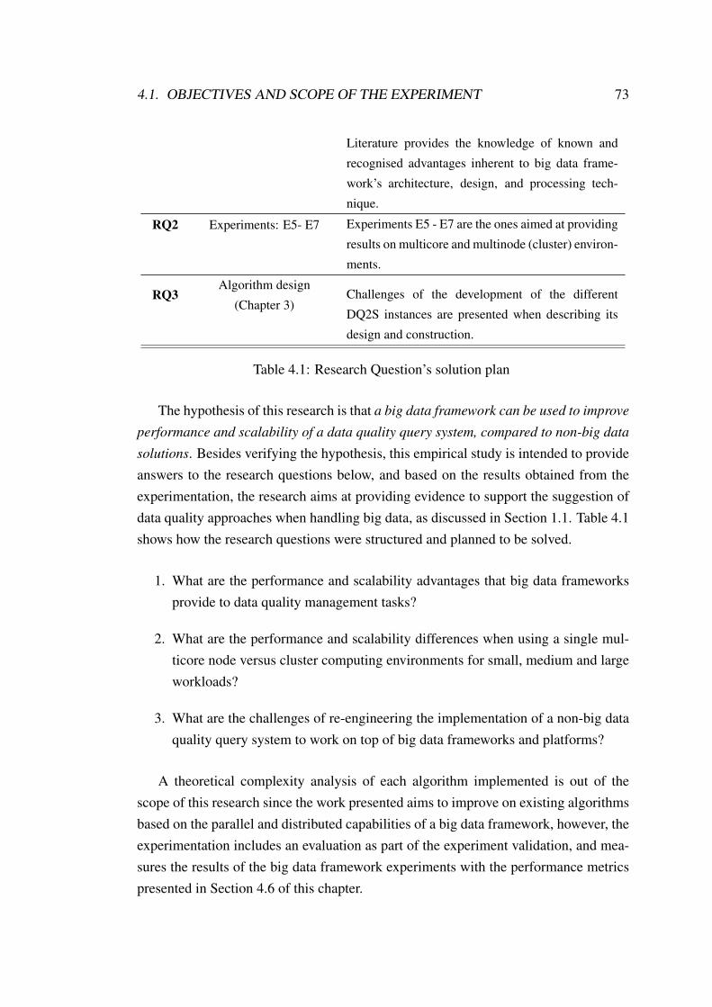
4.1. OBJECTIVES AND SCOPE OF THE EXPERIMENT 73
Literature provides the knowledge of known and
recognised advantages inherent to big data frame-
work’s architecture, design, and processing tech-
nique.
RQ2 Experiments: E5- E7 Experiments E5 - E7 are the ones aimed at providing
results on multicore and multinode (cluster) environ-
ments.
RQ3Algorithm design
(Chapter 3)Challenges of the development of the different
DQ2S instances are presented when describing its
design and construction.
Table 4.1: Research Question’s solution plan
The hypothesis of this research is that a big data framework can be used to improve
performance and scalability of a data quality query system, compared to non-big data
solutions. Besides verifying the hypothesis, this empirical study is intended to provideanswers to the research questions below, and based on the results obtained from theexperimentation, the research aims at providing evidence to support the suggestion ofdata quality approaches when handling big data, as discussed in Section 1.1. Table 4.1shows how the research questions were structured and planned to be solved.
1. What are the performance and scalability advantages that big data frameworksprovide to data quality management tasks?
2. What are the performance and scalability differences when using a single mul-ticore node versus cluster computing environments for small, medium and largeworkloads?
3. What are the challenges of re-engineering the implementation of a non-big dataquality query system to work on top of big data frameworks and platforms?
A theoretical complexity analysis of each algorithm implemented is out of thescope of this research since the work presented aims to improve on existing algorithmsbased on the parallel and distributed capabilities of a big data framework, however, theexperimentation includes an evaluation as part of the experiment validation, and mea-sures the results of the big data framework experiments with the performance metricspresented in Section 4.6 of this chapter.

74 CHAPTER 4. EXPERIMENT DESIGN
4.2 Data and Tools
The query executed in this experimentation (Timeliness query) requires two differentdatasets, named “Order” and “Status Timeliness QR”, both datasets are in CSV commaseparated format and comprise the input data to the query. A description of its contentand structure can be found in Section 3.1.3. Three different sizes of datasets wereutilised as baseline: 50 000, 100 000, and 1 000 000 rows. The size in bytes of eachdataset used is shown in table 4.2.
Number of rows Name of the datasetsOrder Status Timeliness QR
50 000 4.0MB 3.4MB
100 000 8.0 MB 6.8 MB
1 000 000 84.5 MB 68.9 MB
Table 4.2: Relation of number of rows and size per each input dataset utilised in theexperimentation.
The experiments designed for this study were performed in two different environ-ments. The first one is a commodity machine (desktop PC), and the second one is a36 node cluster with a shared storage architecture. The cluster utilised in this studyis the Data Processing Shared Facility at the University of Manchester (DPSF), fromwhich this study utilises 5 of its nodes as to deploy a Spark Cluster. The DPSF clusterutilises the Sun Grid Engine (SGE) to coordinate and schedule the execution of taskssubmitted by the users through batch scripting, aimed at managing the resources andprocesses in a fair and efficient way. The cluster is based on a Lustre file system, a scal-able and optimised software commonly used for High Performance Computing (HPC),known for its usage on supercomputers around the world, with “hundreds of gigabytesper second (GB/sec) of I/O throughput” [98]. Lustre enables access to distributed dataas if it was local, even when in reality, the storage disks are placed physically in furtherlocations, and allows the operation of different processes at the same time on shareddata without interference, avoiding resource contention, and providing coherency onthe data if modified simultaneously; Lustre achieves concurrency support and cachecoherence through its distributed lock manager (LDLM) [98]. The hardware specifi-cation for the desktop PC and the DPSF cluster is shown in Table 4.3, and a summaryof the tools required for the experiments is presented in Table 4.4.

4.2. DATA AND TOOLS 75
Despite the desktop machine being a dual boot one, the experiments were per-formed on the Linux OS, a Fedora 20, with a HDD partition of 500GB. The tools andtechnologies selected are the common ones used for data quality and data wrangling,as well as the most popular, stable and compatible with older and newer versions atthis time.
PC DPSF
No. of nodes 1 5
Operative System(OS)
64-bit dual boot Windows 7
and Linux Fedora 20CentOS Linux release 7.2.1511
CPUIntel(R) Core(TM)
i7-4790 @3.60GHz
Intel(R) Core(TM)
E5-2640 v3 @2.6GHz
No. of physicalCPU cores per node
4 with Hyper
Threading technology
8 with Hyper
Threading technology
Total availableCPU cores per node
8 16
RAM per node 16 GB 512 GB
Total Storage 1TB HDD @7200 RPM650 TB of Lustre-based
scratch storage
Table 4.3: Hardware specification of the desktop machine (PC) and the cluster (DPSF)utilised in the experimentation.
ToolWhere
applicableUsage withinthe research
Datasets based on the business
processes of a e-Business seller
company, the same data used for
the testing the original DQ2S.
PC & DPSF
These are the input data to the
algorithms required to execute the
Timeliness query.
The original Java code from the
DQ2S, provided by the
corresponding authors [26].
PCConforms the baseline of the
performance metrics comparison.
The Java 1.7.0 71 version. PCUsed to execute the original set of
DQ2S algorithms.

76 CHAPTER 4. EXPERIMENT DESIGN
The last major version in the 2.x
series: Python 2.7.12PC & DPSF
Used to execute the Python DQ2S
and the Optimised Python DQ2S
version of the original set of
algorithms.
The Pandas library version 0.17.1 PC & DPSF
Used to execute the Optimised
Python DQ2S version of the
original set of algorithms.
The version 1.6.2 of the Apache
Spark Framework, released on June
25, 2016, with the pre-built
package for Hadoop 2.6 and later.
PC & DPSF
Used to execute the PySpark DQ2S
version of the original set of
algorithms.
Table 4.4: Tools used in the empirical evaluation of the research
4.3 Setup: Spark Cluster and Application Settings
4.3.1 The Apache Spark Local Mode
The Apache Spark big data framework was created to be utilised on a cluster archi-tecture, but it can still it can be set in a called “Local mode”. This implementationdoes not require a cluster manager to schedule the work required to perform the com-putations, and although this Local mode is not meant to offer all of Spark’s completeconfiguration, yet it provides the parallel computation benefit as well as the RDD datastructure, which is one of the Spark’s most valuable asset.
In Local mode, there is no such thing as workers. The driver program becomesalso the executor, and the task scheduling and the tasks execution happens within thesame JVM; in this mode, parallel processing is achieved by multi-threading not reallyby the whole cluster executors, workers and cluster manager process as it is done on areal cluster mode (either Standalone, YARN or Mesos).
To set the number of tasks that a single machine with Local mode should processat the same time, the master address needs to be set to local[n], where n is the num-ber of tasks the framework will handle simultaneously (number of threads), generallyreferred to as “cores”, and as mentioned in Section 3.2.4, general best practice is to setn to the number of available cores.
A cluster mode can be started on a single machine, however, this is commonly

4.3. SETUP: SPARK CLUSTER AND APPLICATION SETTINGS 77
not recommended unless having a large capacity hardware because a cluster modewill cause a single machine to run several JVMs, provoking an overhead due to theJVMs initiation, generating in this way more processes than the Local mode generates,thus becoming more costly in terms of CPU usage, and therefore runtime, as the OSwill need to handle more processes. When not having a cluster, or a large capacitymachine, the Local mode provides an option to utilise Apache Spark taking the mostof the resources available to process a Spark application with a simpler deployment.Spark Local mode was used on some of the experiments performed with the big dataframework on the desktop machine described in Table 4.3, aimed at exploring the Localmode behaviour on a commodity machine for the Timeliness query.
4.3.2 The Apache Spark Standalone Mode
Another Spark mode is its implementation and usage on a cluster, which is the realfocus of the framework. It is important to point out that Standalone mode cannot becalled like that unless the Spark’s cluster manager is used. The role of the “cluster man-ager” serves a purpose within job submission on a cluster by scheduling the resourcesrequested, utilising the workers to create executors for the driver and communicatingthe workers and executors availability to the driver process, even if only one user isgoing to utilise the cluster or only one application will be submitted, although this isnot likely to be the case when Spark is used on a cluster.
For this research, to execute the Timeliness query with the PySpark code, denom-inated as the “application”, the TimelinessQuery class needs to be submitted to theSpark cluster. The applications submitted to Spark run through Spark’s master-slavearchitecture, where the set of processes corresponding to the application is coordi-nated by the driver program, the one containing the SparkContext object declaration,as shown in Section 3.2.4. This research uses the Standalone manager since it is theone created specifically for Spark and this investigation seeks to conduct an evaluationon the big data framework in isolation, without further aid from other technologies,in order to analyse Spark’s capabilities. This decision on the cluster manager is whatgives the name to a “Standalone mode” when talking about a Spark cluster.
There are three locations in which Spark configurations can be made [129], sum-marised in Table 4.5:
• Application parameters can be set directly on a SparkConf instance, passed

78 CHAPTER 4. EXPERIMENT DESIGN
to the SparkContext object, where the SparkConf object contains informa-tion about the application that is going to be executed within Spark, for example,the master’s node address, the application name or the home directory path.
There are three ways of setting Spark properties using the SparkContext object:embedded in the source code of an application, using flags to the pyspark-submitcommand used to submit an application to the framework or written on the./spark home directory/conf/spark-defaults.conf file, which are takenby Spark, following that order priority.
Using flags makes possible to submit spark-defaults.conf parameters, byusing the --conf flag, followed by the spark parameter. E. g. -- conf spark.
driver.cores=2.
• Per-machine and cluster settings can be set statically on the configurationsfiles, where spark-env.sh is the environmental variables file, used to specifythe details of the version number used for Java and Python, and set the num-ber of executors, its number of cores to be used on each machine, as well asmaximum memory. This file is needed by the cluster launching scripts foundin ./spark-home-directory/sbin path, named start-master.sh, start-slaves.sh and start-all.sh, which starts the cluster and/or its slaves oncesubmitted through Spark.
To specify where Spark should start a slave node, the slaves (without any kindof extension) file is used, taken by the start slaves launching script. All of theconfiguration files can be found in ./spark home directory/conf path.
• Logging through log4j Apache logging service, to specify how the cluster col-lects and presents logged data, by adding a file that should be named lo4j.
properties in the conf directory. Log4j is a logging and tracing API, whichsupports a debugging method by looking at the logs created by the application.In Spark, for example, it can be used to set the console as the place which every-thing must be logged to or to set the default log level.
The above mentions examples of the relevant configurations to this research, however,an exhaustive list of settings available for Spark can be found in [129].
Configurationtype
File / Placeto utilise
Purpose Location

4.4. EXPERIMENT PROCEDURE 79
Application
parameters.
SparkConf
instance.
Set spark properties to
access the cluster. E.g.
Master’s node address,
application name, or
home directory path.
Source code of an application,
flags in submission or
./spark home directory/conf/
spark-defaults.conf
Cluster
settings.
spark-env.sh
Set environmental
variables. E.g. Java and
Python version, number
of executors, etc.
./spark home directory/conf
/spark-env.sh
slavesSpecify address to start
a slave node.
./spark home directory/conf
/ slaves
Logging lo4j.properties
Specify how the cluster
collects and presents
logged data.
./spark home directory/conf/
log4j.properties
Table 4.5: Spark configuration locations
For this study, three files from the Spark directory were edited with different pa-rameters on each experiment: spark-env.sh, spark-defaults.conf, and slaves.The content set to each file per experiment is described in Section 4.4 of this Chapter.
4.4 Experiment Procedure
Experiment Rationale
E1 From E1 to E4, will be used as a baseline to be able to compare results with the
other Experiments. This will conform the analysis of how DQ2S scales and
performs using non-big data implementations.E2E3E4
E5 E5 and E6 support the analysis of a big data framework’s capabilities when
being used on a single multicore machine, and provides the information to
compare results from E1-E4 (non-big data) with a big data solution.E6E7
E8 E8 supports the analysis of the big data framework behaviour in a cluster
environment, and accompanied by E9, offers an overview of the advantages
that a big data framework provides when processing different workload sizes.E9
Table 4.6: General overview of the experiment’s aim

80 CHAPTER 4. EXPERIMENT DESIGN
Experiment Environment Number of runtimes recordedNumber of
averages recorded
E1 PC 15 (5 per input size - 5 x 3) 3
E2 PC 15 (5 per input size - 5 x 3) 3
E3 PC 15 (5 per input size - 5 x 3) 3
E4 PC 5 per succesful input size 1
E5 PC
120 (one per input size per
configuration - 3 x 8)
(5 per single runtime - 5 x 24)
24
E6 PC
120 (one per input size per
configuration - 3 x 8)
(5 per single runtime - 5 x 24)
24
E7 PC
120 (one per input size per
configuration - 2 x 12)
(5 per single runtime - 5 x 24)
24
E8 Cluster
60 (one per input size per
configuration - 3 x 4)
(5 per single runtime - 5 x 12)
12
E9 Cluster 15 (5 per input size - 5 x 3) 3
Table 4.7: Number of runtimes and averages collected by experiment.
To tackle the research questions, the testing involved the execution of the Time-liness query under different environmental settings. These settings depend on threevariables: the Timeliness query instances (described in Chapter 3), the dataset file size,and the usage of a desktop machine and a cluster. The experiments were separated intonine different ones, in a way that each experiment could have its own delimited andclear set of results to be later compared and correlated altogether, these experimentsare presented below. All the programming classes mentioned are described in Chapter3. A summary of the experiment’s aims and an overview of the recorded quantity of re-sults obtained from the nine different experiments is shown in Table 4.6 and Table 4.7,respectively. Each run indicated utilised both orderT and statusTimelinessQR datasetsof the same size, for example, when indicating a run of 50 000 000 rows, both orderT
and statusTimelinessQR contain 50 000 rows each one. Runtimes were recorded inmilliseconds and 5 times as described in Table 4.7, the average result was utilised toassure a higher level of precision considering that executions in a system do not run

4.4. EXPERIMENT PROCEDURE 81
for the same exact milliseconds due to Operative System’s (OS) processes that are notuser controlled.
E1. Original Java DQ2S experiment - PC
This experiment was executed on the desktop machine, and aims to show howthe original DQ2S configuration implemented with Java scales and performs.For this experiment, each dataset size (50 000, 100 000 and 1 000 000 rows)was used as input for the Java program. The following procedure was utilised torecord the results:
(a) Open a Linux terminal.
(b) Place to the folder containing the Java classes.
(c) Create the classes to execute typing: javac TimelinessQuery.java
(d) Execute the TimelinessQuery class typing: java TimelinessQuery
(e) Discard the first run, known as “cold run”, in which data is loaded into thecache of the machine.
(f) Register the runtime printed out in console, aided by the Timing class.
(g) Repeat (d) and (f) five times.
(h) Calculate the average time of the five registered times.
E2. Python DQ2S experiment - PC
This experiment was executed on the desktop machine, and aims to show howPython DQ2S scales and performs in comparison to the Java DQ2S instance.This was done by gathering the runtime results from the Python DQ2S executedover each dataset size (50 000, 100 000 and 1 000 000 rows), utilising the fol-lowing procedure, and compared later with the results from Experiment 1 (E1 inthis chapter):
(a) Open a Linux terminal.
(b) Locate to the folder containing the correspondent Python classes.
(c) Execute the TimelinessQuery class typing: python TimelinessQuery.py
(d) Discard the first run, known as “cold run”.
(e) Register the runtime printed out in console, aided by the Timing class.
(f) Repeat (c) and (e) five times.

82 CHAPTER 4. EXPERIMENT DESIGN
(g) Calculate the average time of the five registered times.
E3. Optimised Python DQ2S experiment - PC
The aim of this experiment is to explore how the Optimised Python DQ2S scalesand performs in comparison to the Python DQ2S and the Java DQ2S. Eachdataset size (50 000, 100 000 and 1 000 000 rows) was used as input 6 timesper size, collecting 5 runtimes per dataset size, discarding the first run each time.This experiment followed the same procedure as Experiment 2 (E2 in this chap-ter) since this is an instance developed also in Python language with the imple-mentation of a scientific library, as described in Chapter 3.
E4. Optimised Python DQ2S maximum capacity experiment - PC
This experiment aims at finding up to how many rows the Optimised PythonDQ2S can process the Timeliness query successfully on the desktop machine.Taking into account that how big is big data could be thought as the size inwhich using “traditional techniques” for the processing is no longer an option.For this experiment a 5 000 000 rows dataset was utilised as first attempt toprocess a larger dataset than the 1 000 000 rows one (baseline as described inSection 4.2). This value provided the knowledge to whether or not that was alarge enough dataset, so the volume could be increased on a 5 000 000 rowsbasis, or decreased on 1 000 000, as follows:
(a) Open a Linux terminal.
(b) Locate to the folder containing the correspondent Python classes.
(c) Use an input data set of 5 000 000 rows.
(d) Execute the TimelinessQuery class typing: python TimelinessQuery.py
(e) Discard the first run, known as “cold run”.
(f) Repeat (d) and if the execution completes to the end successfully, add5 000 000 rows to the input data set and repeat from (d).
(g) Once a failure is reached, subtract 1 000 000 rows to the input dataset thatcaused the failure.
(h) Repeat (d) and (e), and keep subtracting 1 000 000 rows until the input datasize causes a successful run.

4.4. EXPERIMENT PROCEDURE 83
(i) After (h) is completed (a input data size was found by reducing 1 000 000rows each time), add 500 000 rows to the last known successful dataset andrepeat (d) and (e).
(j) If the input data set size of (i) was successful, execute (k), otherwise de-crease by 500 000 rows the dataset and execute (d), (e) and continue with(k).
(k) Register the number of rows of the input data set.
(l) Register the runtime printed out in console, aided by the Timing class.
(m) Repeat (d) and (l) five times.
(n) Calculate the average time of the five registered times.
E5. PySpark DQ2S Standalone mode in single machine experiment - PC
The Standalone mode was not designed to be used on a single machine, as de-scribed in Section 4.3.2, however, it is a common beginner’s mistake to imple-ment it that way, risking at having a wrong implementation that could offer awrong impression of a big data framework performance. Another common mis-take is to create more workers in order to have more executors, since for SparkStandalone mode it is not very clear how to set more than one executor perworker, and also because on Spark’s versions below 1.4.0, it was not possible tohave more than one executor per worker. This experiment sets one executor perworker to explore what would happen if a Standalone mode is implemented andintended to be used for the DQ2S in a single multicore machine, with the circum-stances mentioned (one executor per worker, constrained to physical cores). Theresults of this experiment will form part of the supporting information to analysewhether a cluster is mandatory to take the most of Spark, as well as contribute tothe insights of the big data framework behaviour in a desktop environment (PC).
The steps followed to start-up the cluster used on this experiment are detailedin Appendix B, Section B.2, and the actions used to submit the PySpark ap-plications can be found in Section B.3. For this experiment, three files fromthe Spark directory were edited: spark-env.sh, spark-defaults.conf, andslaves. All of the settings are options used by the Standalone cluster, whereit was considered a total memory of 14GB, by a naive consideration of keep-ing 2GB for OS processes, and 4 physical cores. The number of physical coresprovided a total of 8 configurations, as described below.

84 CHAPTER 4. EXPERIMENT DESIGN
The submission requires several parameters to be set, including the applicationname, the master node address, number of workers per node, number of execu-tors per worker and its corresponding memory and number of simultaneous tasksan executor will handle (known as “cores”). The application name and the mas-ter’s node address was defined in the code of the programs, this is not practicalwhen using different applications or in a cluster where it might require a moredynamic update of those parameters, but for this experiment, since it was doneusing only one computer, it did not produce any drawback.
1. The content of the spark-env.sh file was set as follows:
export SPARK_WORKER_MEMORY=3.5,4.7,7,14g
export SPARK_EXECUTOR_MEMORY=3.5,4.7,7,14g
export SPARK_WORKER_INSTANCES=1,2,3,4
export SPARK_WORKER_CORES=1,2,3,4
export SPARK_WORKER_DIR=/local_drive/sparkdata
• SPARK WORKER MEMORY is used to set how much total memorymust be reserved for each executor, since one executor is created perworker, according to the given parameters of the worker, as explainedin Section 3.2.4. This was fixed to 3.5, 4.7, 7 and 14 GB in differenttimes, constrained by the number of workers set. Those numbers wereobtained based on the total amount of memory available and the num-ber of workers set, hence, when the testing was executed with 2 work-ers, the memory was divided by 2, thus, SPARK WORKER MEMORYhas a value of 7GB.
• SPARK EXECUTOR MEMORY allows to specify how much of theworker’s reserved memory must be given to each executor. This pa-rameter was set to be the same value as SPARK WORKER MEMORY,in order to have always one executor per worker. Both SPARK WORKERMEMORY and SPARK EXECUTOR MEMORY do not accept val-
ues different to integers, therefore, to set 3.5 and 4.7GB, it was doneusing its equivalent integer value in MB. E.g. 3584M instead of 3.5g(Spark utilises a notation of M for MB, and g for GB in the spark-env.shsettings).

4.4. EXPERIMENT PROCEDURE 85
• SPARK WORKER INSTANCES defines the number of worker pro-cesses with one executor process each one. The evaluation was exe-cuted using from 1 to 4 workers each time. More than 4 workers wasnot tested because of the availability of 4 cores; 5 workers require atleast the allocation of 5 cores, one per worker.
• SPARK WORKER CORES sets the number of simultaneous tasks tobe handled per executor on each worker. In this case the value usedwas selected according to the number of workers used. For example,when using 1 worker, it use from 1 to 4 cores each time, but having2 workers can only use 1 or 2 cores each since using 3 cores for 2workers means 6 cores would be required.
• SPARK WORKER DIR is used to specify the working directory ofthe worker processes, in this case it was used the local drive and adirectory named “sparkdata”.
2. The content of spark-defaults.conf was configured to enable visibilityof the application executions log after the work is finished. The propertiesset were the following:
spark.eventLog.enabled true
spark.eventLog.dir //local_drive/sparkLogs
Where eventLog.enable sets to true or false to see the information afterthe application is finished and the eventLog.dir property sets the path tothe folder where the logs should be saved.
3. Finally, the slaves file, contains only the word “localhost”, to specify thatthe workers should be started locally, since the implementation is deployedin the same machine.
The procedure to execute this experiment is the following one:
(a) Turn on the Standalone Spark cluster by starting the master and slavesnodes.
(b) In the files with the cluster settings, modify the number of workers, coresand allocated memory as required.
(c) Manually submit the TimelinessQuery class to the Spark cluster, using:

86 CHAPTER 4. EXPERIMENT DESIGN
bin/spark-submit --packages com.databricks:spark-csv_2.11:1.3.0 \
TimelinessQuery.py TimelinessRun_1 outputResults_1
Where TimelinessRun 1 is the name of the application, utilised by thecluster deployment to identify the application, useful when the Standaloneor any other cluster mode is used by many users or to submit several ap-plications; and outputResults 1 is the name of the folder in which Sparkwill save the results, this name could be any name.
(d) Register the runtime printed out in console, aided by the Timing class.
(e) Discard the first run, known as “cold run”.
(f) Repeat (c) and (d) five times per each set of parameters.
(g) Calculate the average time of the five registered times.
E6. PySpark DQ2S Local mode in single machine experiment - PC
The aim of this experiment is to show how Spark in Local mode performs andscales in a multicore machine. The input sizes utilised for this experiment arealso 50 000, 100 000 and 1 000 000 rows. This experiment comprises 6 execu-tions per input data set size for the following variables, executing a total of 12different configurations, setting from 1 to 8 threads for the n value in local[n],where an execution without any kind of parallelisation is achieved by settingthe Spark master parameter to local[1]. This was set up to 8 because of theavailable cores in the machine. This experiment and all of the ones performedusing the Local mode, utilised a driver memory of 12GB, based on Spark’s rec-ommendation of utilising up to 75% of the total available memory [46]. Theprocedure was followed as shown below:
(a) Open a Linux terminal.
(b) Locate to the Spark’s home directory.
(c) Manually submit the TimelinessQuery class to Spark using:
sbin/spark-submit TimelinessQuery.py
--packages com.databricks:spark-csv_2.11:1.3.0
--driver-memory 12g --master local[n]
with n being from 1 to 8.
(d) Register the runtime printed out in console, aided by the Timing class.
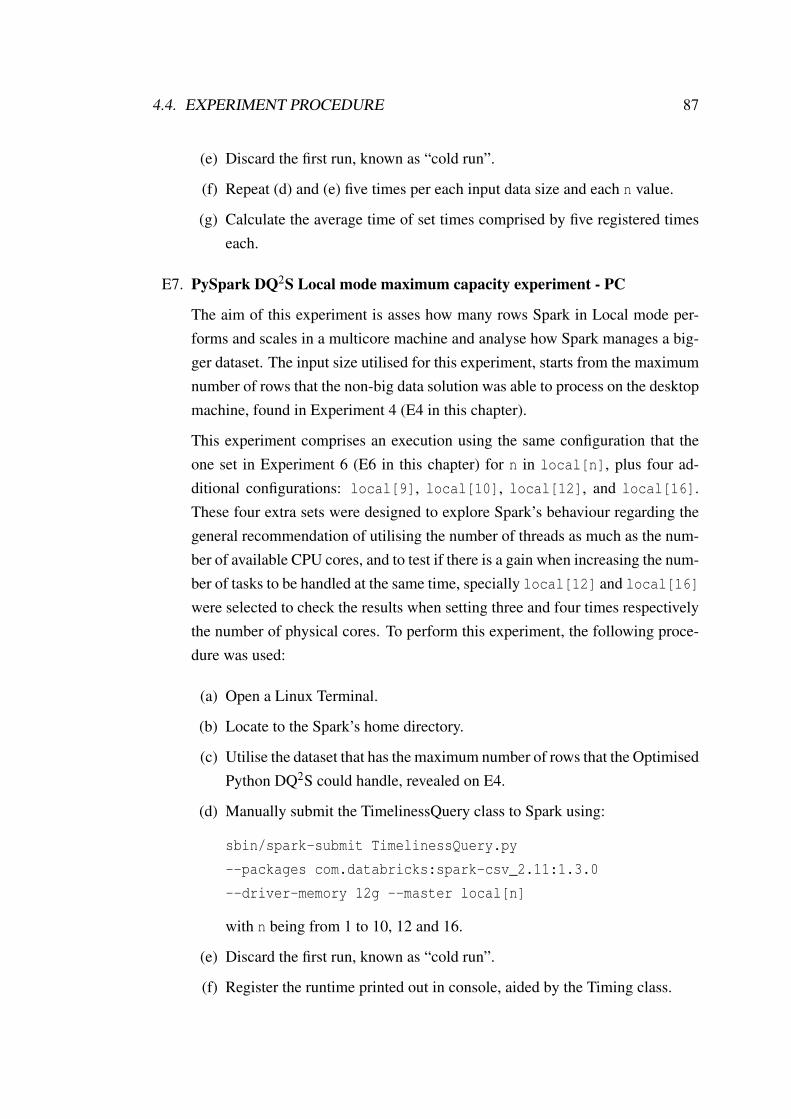
4.4. EXPERIMENT PROCEDURE 87
(e) Discard the first run, known as “cold run”.
(f) Repeat (d) and (e) five times per each input data size and each n value.
(g) Calculate the average time of set times comprised by five registered timeseach.
E7. PySpark DQ2S Local mode maximum capacity experiment - PC
The aim of this experiment is asses how many rows Spark in Local mode per-forms and scales in a multicore machine and analyse how Spark manages a big-ger dataset. The input size utilised for this experiment, starts from the maximumnumber of rows that the non-big data solution was able to process on the desktopmachine, found in Experiment 4 (E4 in this chapter).
This experiment comprises an execution using the same configuration that theone set in Experiment 6 (E6 in this chapter) for n in local[n], plus four ad-ditional configurations: local[9], local[10], local[12], and local[16].These four extra sets were designed to explore Spark’s behaviour regarding thegeneral recommendation of utilising the number of threads as much as the num-ber of available CPU cores, and to test if there is a gain when increasing the num-ber of tasks to be handled at the same time, specially local[12] and local[16]
were selected to check the results when setting three and four times respectivelythe number of physical cores. To perform this experiment, the following proce-dure was used:
(a) Open a Linux Terminal.
(b) Locate to the Spark’s home directory.
(c) Utilise the dataset that has the maximum number of rows that the OptimisedPython DQ2S could handle, revealed on E4.
(d) Manually submit the TimelinessQuery class to Spark using:
sbin/spark-submit TimelinessQuery.py
--packages com.databricks:spark-csv_2.11:1.3.0
--driver-memory 12g --master local[n]
with n being from 1 to 10, 12 and 16.
(e) Discard the first run, known as “cold run”.
(f) Register the runtime printed out in console, aided by the Timing class.
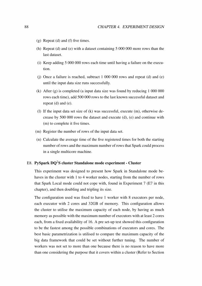
88 CHAPTER 4. EXPERIMENT DESIGN
(g) Repeat (d) and (f) five times.
(h) Repeat (d) and (e) with a dataset containing 5 000 000 more rows than thelast dataset.
(i) Keep adding 5 000 000 rows each time until having a failure on the execu-tion.
(j) Once a failure is reached, subtract 1 000 000 rows and repeat (d) and (e)until the input data size runs successfully.
(k) After (g) is completed (a input data size was found by reducing 1 000 000rows each time), add 500 000 rows to the last known successful dataset andrepeat (d) and (e).
(l) If the input data set size of (k) was successful, execute (m), otherwise de-crease by 500 000 rows the dataset and execute (d), (e) and continue with(m) to complete it five times.
(m) Register the number of rows of the input data set.
(n) Calculate the average time of the five registered times for both the startingnumber of rows and the maximum number of rows that Spark could processin a single multicore machine.
E8. PySpark DQ2S cluster Standalone mode experiment - Cluster
This experiment was designed to present how Spark in Standalone mode be-haves in the cluster with 1 to 4 worker nodes, starting from the number of rowsthat Spark Local mode could not cope with, found in Experiment 7 (E7 in thischapter), and then doubling and tripling its size.
The configuration used was fixed to have 1 worker with 8 executors per node,each executor with 2 cores and 32GB of memory. This configuration allowsthe cluster to utilise the maximum capacity of each node, by having as muchmemory as possible with the maximum number of executors with at least 2 coreseach, from a fixed availability of 16. A pre set-up test showed this configurationto be the fastest among the possible combinations of executors and cores. Thebest basic parametrization is utilised to compare the maximum capacity of thebig data framework that could be set without further tuning. The number ofworkers was not set to more than one because there is no reason to have morethan one considering the purpose that it covers within a cluster (Refer to Section
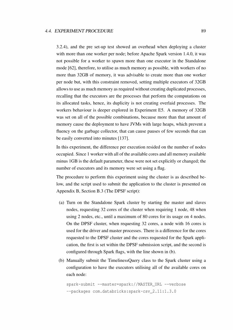
4.4. EXPERIMENT PROCEDURE 89
3.2.4), and the pre set-up test showed an overhead when deploying a clusterwith more than one worker per node; before Apache Spark version 1.4.0, it wasnot possible for a worker to spawn more than one executor in the Standalonemode [62], therefore, to utilise as much memory as possible, with workers of nomore than 32GB of memory, it was advisable to create more than one workerper node but, with this constraint removed, setting multiple executors of 32GBallows to use as much memory as required without creating duplicated processes,recalling that the executors are the processes that perform the computations onits allocated tasks, hence, its duplicity is not creating overlaid processes. Theworkers behaviour is deeper explored in Experiment E5. A memory of 32GBwas set on all of the possible combinations, because more than that amount ofmemory cause the deployment to have JVMs with large heaps, which prevent afluency on the garbage collector, that can cause pauses of few seconds that canbe easily converted into minutes [137].
In this experiment, the difference per execution resided on the number of nodesoccupied. Since 1 worker with all of the available cores and all memory availableminus 1GB is the default parameter, these were not set explicitly or changed; thenumber of executors and its memory were set using a flag.
The procedure to perform this experiment using the cluster is as described be-low, and the script used to submit the application to the cluster is presented onAppendix B, Section B.3 (The DPSF script):
(a) Turn on the Standalone Spark cluster by starting the master and slavesnodes, requesting 32 cores of the cluster when requiring 1 node, 48 whenusing 2 nodes, etc., until a maximum of 80 cores for its usage on 4 nodes.On the DPSF cluster, when requesting 32 cores, a node with 16 cores isused for the driver and master processes. There is a difference for the coresrequested to the DPSF cluster and the cores requested for the Spark appli-cation, the first is set within the DPSF submission script, and the second isconfigured through Spark flags, with the line shown in (b).
(b) Manually submit the TimelinessQuery class to the Spark cluster using aconfiguration to have the executors utilising all of the available cores oneach node:
spark-submit --master=spark://MASTER_URL --verbose
--packages com.databricks:spark-csv_2.11:1.3.0

90 CHAPTER 4. EXPERIMENT DESIGN
--executor-memory 32G --executor-cores 2 TimelinessQuery.py
Where MASTER URL is the URL of the master node, set by the DPSF script.
(c) Register the runtime printed out in console, aided by the Timing class.
(d) Discard the first run, known as “cold run”.
(e) Repeat (b) and (c) five times per each set of parameters.
(f) Calculate the average time of the five registered times per different numberof nodes.
E9. Optimised Python DQ2S cluster experiment - Cluster
This experiment shows how the optimised Python DQ2S scales and performs inthe cluster, using the input data sizes utilised in Experiment 8 (E8 in this chapter).The procedure for this experiment is the same as described in Experiment 2 (E2in this chapter), but performed in the cluster instead of in a desktop machine.
4.5 Algorithm Comparison
The results obtained from the executions defined above were analysed according to thefollowing observations, which were designed to avoid having comparisons betweenthe different instances of the DQ2S being advantageous one over another due to itsinherent structure, power given by number of cores, or degree of parallelism, this is,having comparisons based on platform utilisation and not in algorithm design (Refer toSection 2.4 for details of platform and algorithm design scalability approaches). Thepurpose of the following comparisons designed is also to organise the results in such away them could offer an insight that can support the hypothesis.
C1. The original DQ2S Java program (E1) compared with its equivalent DQ2Sdeveloped using Python (E2).
These programs support a comparison of the same algorithm written in differentlanguages, without any kind of parallelisation implemented. This comparisonwas thought to offer an insight regarding Python against the original DQ2S de-veloped with Java, with regards to its performance and scalability.
C2. The Python DQ2S program (E2) compared with the Optimised Python ver-sion of it (E3).

4.5. ALGORITHM COMPARISON 91
These instances were thought to be a basis for showing the performance obtainedfrom implementing the data frames library without a big data framework. Theresults of the Optimised Python version of DQ2S provide a reference for theresearch on scaling with big data frameworks.
C3. The Optimised DQ2S Python program (E3) compared with the PySparkDQ2S program in Local mode (E6).
This comparison was designed to show measurements that led to an analysis ofthe impact caused by the usage of a big data framework, having as baseline theresults from the comparison mentioned in C2. The outcome of this comparisonwould be to inspect the performance obtained from the usage of Apache Sparkimplemented within a single multi-core machine, leading to know the actual andquantifiable impact obtained from the usage of a big data framework for this andsimilar use cases.
C4. The maximum number of rows processed by the Optimised DQ2S Pythonprogram (E4) compared with the PySpark DQ2S program in Local mode(E7).
These results were designed to explore the behaviour of the big data frameworkwhen processing the maximum data volume that the DQ2S instance without par-allelism could cope with, aimed at discovering if the framework can offer anyadvantage with regards to processing capacity, focused on the volume character-istic of big data, as well as to asses its scalability and performance comparingthese two instances when processing similar workloads (volume).
C5. The PySpark DQ2S program in Standalone mode (E5) compared with aPySpark DQ2S in Local mode (E6), both in a single machine.
Although the Standalone mode is not designed to be utilised in a single core ma-chine, it could be the case that it is used this way as it is possible to do it, hence,this comparison aims at exploring the differences between Local and Standalonemode implemented in a single machine and gather insights about their perfor-mance and general behaviour when processing the same datasets.
C6. The PySpark DQ2S program in Local mode (E7) compared with a PySparkDQ2S used in a cluster under Standalone mode (E8).
This comparison was designed to explore the extent to which a cluster envi-ronment provides significant advantages over a multicore commodity hardware.

92 CHAPTER 4. EXPERIMENT DESIGN
The purpose of this comparison is to analyse if a cluster is mandatory to considera big data framework a suitable option for big data processing.
C7. The PySpark DQ2S program in Standalone mode (E8) compared with aOptimised Python DQ2S version executed on the cluster (E9)
This final comparison was designed to offer a view of how a non-big data so-lution works under a cluster environment, therefore, to discard or include thearchitecture as crucial in terms of scalability and performance results.
4.6 Experiment Evaluation
The executions were monitored to asses the performance in terms of the metrics definedfor parallel algorithms, which are described in detail in Section 4.6.1, and calculatedusing the formulas described in the same section, which require only the runtime of theexecution. A second part of the experiment evaluation includes a validity assessmentto support the apparent conclusions obtained from the results, as well as an descriptionof how threats to validity were approached, described in Section 4.6.2.
4.6.1 Performance Metrics
The cluster created has a shared memory in a shared disk architecture, having availablethe data stored in the only one Hard Disk in use, and accessible for all the membersof the cluster globally, as well as the memory available. Still a parallel architecture,it was needed to use Performance Metrics specifically designed to measure certaincharacteristics available for parallel programs.
The most common metrics for performance on parallel algorithms [73, 3, 28, 4,118, 114] were used to support the performance analysis, based on the comparisonsdesigned and described in Section 4.5. The information required by the performancemetrics used for this research are the following:
• Serial runtime (TS). The measurement of the time elapsed between the begin-ning and the end of the fastest known serial algorithm that solves the problem.
• 1 Core serial runtime (T(1)). The measurement of the time elapsed betweenthe beginning and the end of a parallel algorithm executed on a single core.

4.6. EXPERIMENT EVALUATION 93
• Parallel runtime (TP). The measurement of the time elapsed between the be-ginning and the end of a parallel algorithm executed on more than one core. Thistime is composed by 3 different components: the time spent on the computation,the cores communication time, and the idle time which is when any processor isworking but still has not finished.
• Number of cores (p). The number of processing elements on which the parallelalgorithm is executed. For this study the processing elements are the cores set asdescribed in Section 4.4.
The performance metrics considered for this study are as follows:
1. Speedup (S). Meant to measure the performance gain of a parallel program whensolving the same problem over the sequential implementation one. In an idealparallel system, speedup is equal to the number of cores used, however, it isusually lower than p.
There are more than one approach towards measuring speedup: Relative, Real,Absolute, Asymptotic and Asymptotic relative [114, 123]. This study occupiesthe ones that are valid and entirely applicable to the design and scope of theresearch, as follows:
• Real Speedup (rS). This speedup requires the sequential time TS from thefastest serial algorithm available to be compared against time obtained fromthe parallel algorithm over more than one core. This speedup is calculatedusing:
rS =T ST P
. (4.1)
• Relative Speedup (rtS). Calculates the speedup regarding TS as the paral-lel execution time from the algorithm run over one core T(1). This is madeto consider the inherent parallelism of the parallel algorithm that is beingassessed. The formula utilised to calculate the relative speedup is:
rtS =T (1)T P
. (4.2)
The aim of this calculations is to isolate the benefit from parallelism given by asingle parallel processing unit and the fastest sequential algorithm.

94 CHAPTER 4. EXPERIMENT DESIGN
2. Efficiency (E). Closely related to speedup, measures the resource utilisationgiven the number of parallel units used. Efficiency is constrained by the non-sequential operations performed by the cores, this is, how much of the entireprogram is parallelised. This metric is defined as the ration between the speedupvalue and the number of cores used.
The aimed efficiency for parallel systems is equal to one, but it is, in practice,usually between zero and one; an “scalable algorithm” tend s to increase itsefficiency when p grows. Efficiency is calculated by:
E =Sp
=T S
T P∗ p. (4.3)
• Real Efficiency (rE). Calculates the efficiency with the correspondent rSvalue, as follows:
rE =rSp
=T S
T P∗ p. (4.4)
• Relative Efficiency (rtE). Utilises either rtS or T(1) for the TS value inthe Efficiency formula (E), as follows:
rtE =rtSp
=T (1)
T P∗ p. (4.5)
4.6.2 Validity Evaluation
The design of the experiment is in general a one factor with two treatments model, withsome comparisons having more than two treatments. The factor is the dataset, whichis the same on its content, differentiated only by its size. The treatments are the DQ2Sinstances; an instance with different parameters is considered as another treatment, forexample, a PySpark on Local mode is a different treatment to a PySpark instance onStandalone mode.
When evaluating the results validity, there are four classifications assessed [17]:

4.6. EXPERIMENT EVALUATION 95
• Conclusion validity, concerning the conclusions based on the results obtained.
• Internal validity, to ensure the effect of the treatment is in fact caused by thetreatment and no other factor.
• Construct validity, to be sure the treatment is what it is supposed to be, andworks as it is expected to work according to the experiment description andtheory related to the treatment.
• External validity, to check to which extent the results obtained can lead to ageneralisation and real-world application.
There are recognised threads to validity [17], correspondent to the classificationslisted above. The threats applicable to this study were approached as shown in Tables4.8, 4.9, 4.10 and 4.11.
Conclusion validity
Threat Description How it was addressed
Fishing
results
This threat refers to the action of
looking for specific or favourable
results, discarding the inconve-
nience of some data.
Reproducibility details of the research
offers a support to obtain the re-
sults provided, confirming data gath-
ered was taken from the results as de-
scribed, without discarding data to pro-
duce a desired outcome.
Reliability of
measures
Level of trust in which the val-
ues that constitute the samples
are accurate representations of
the measured events.
A custom instrumentation aided by
code was implemented to measure each
execution runtime without human in-
tervention or subjectivity, assuring the
same mechanism for all of the experi-
ments.

96 CHAPTER 4. EXPERIMENT DESIGN
Random in-
terference in
experimental
settings
There could be factors involved
in the experiment execution that
alter the results, other than the
known or planned.
OS processes as well as other processes
could alter the runtimes if the CPU and
RAM were subject to varying loads not
connected with the experiment, to ad-
dress this, no other applications were
being used while performing the ex-
periments besides the necessary ones
(console, browser and notepad), and
the same applications were used in the
same state when carrying out the exe-
cutions. This is also why more than one
runtime was collected per instance, per
dataset size and per configuration.
Random het-
erogeneity of
subjects
Heterogeneity could lead to hav-
ing abnormal results due to the
heterogeneity of the datasets,
rather than due to the performed
and measured intervention.
This threat is addressed by having the
same dataset involved in all of the ex-
ecutions of the experiments. To min-
imise the trade-off of having a reduced
population, different dataset sizes were
used.
Table 4.8: Conclusion validity threats applicable to the research presented. Details andaddressing approach.
Internal validity
Threats Description How it was addressed
History The risk of time when
the experiment was car-
ried out affecting the re-
sults.
Same version numbers were utilised
for all of the experiments to avoid up-
dates that happened over time affect-
ing the results. No other time situa-
tion is applicable to the research. In
the cluster, time of the day related to
user concurrence does not affect the re-
sults since the nodes were fully utilised
by the experiment, without sharing re-
sources with other users.

4.6. EXPERIMENT EVALUATION 97
Maturation The results can be af-
fected as time passes,
presenting different be-
haviours the first time the
experiment was applied
than the subsequent times.
This threat is applicable because of the
cache mechanism, but it was addressed
flushing the cache each time a new ex-
periment was performed, and the col-
lected runtimes did not take into ac-
count the first result to avoid this threat.
Instrumentation A bad design on the exe-
cution and the way of ob-
taining the data could pro-
vide incorrect values.
This threat is aligned to the reliability
of measures, addressed by implement-
ing a runtime class, described in Chap-
ter 3, which is homogeneous to all of
the instances, does not affects or influ-
ences the results, and is implemented
from the internal code, which increases
accuracy of real processing time, re-
ducing the error of measurement that
could be made, for example, by count-
ing the time including the one spent on
the cluster queue.
Statistical regres-
sion
Classification of experi-
mental groups based on
a known given range, for
example top or bottom re-
sult, which would con-
form a pre-disposition for
further results.
To avoid analysing results based on this
threat, comparisons were designed to
refrain from analysing results based on
unequal, not comparable instances. For
example, results from the cluster with
a 4 node deployment is not comparable
to a desktop PySpark Local mode on its
worse configuration.
Ambiguity about
direction of causal
influence
An issue of unclarity
about identifying the
cause and the effect,
where a result has the
possibility of being either
any of both, or only part
of the cause or the effect.
Homogeneity of the factor to utilise
in the experimentation (the dataset)
avoids variability on each of the exper-
iments, reducing the unknown of con-
sidering if perhaps the factor, not the
treatment, offered the different results.
Table 4.9: Internal validity threats applicable to the research presented. Details andaddressing approach.

98 CHAPTER 4. EXPERIMENT DESIGN
Construct validity
Threats Description How it was addressed
Inadequate pre-
operational de-
scription of con-
structs
Ambiguity and unclarity on the
description of the experiment,
lack of sufficient details to pro-
vide a solid base upon which re-
sults and analysis are described.
This research presents details on the treat-
ments, the factor of the experiment, the proce-
dure and its analysis method, supported by a
rigorous methodology, as described in Chap-
ter 1.
Mono-operation
bias
When the experiment is limited
to few or even only one vari-
able, use case, factor, or treat-
ment, which carries a risk of
having a diminished scope in
which results are valid. The
threat becomes active when this
sub-representation is not consid-
ered or known.
The scope of the research considers its limita-
tions, and avoids overgeneralising results ac-
cordingly.
Mono-method bias Utilising a single measure, or a
single collection method, with
subjectivity involved, could alto-
gether and individually led to bi-
ased results.
Measurements are free of subjectivity in this
research, achieved by a lack of human inter-
pretation on the runtime recorded. The run-
times obtained from the instrumented internal
code were checked against Spark’s Web User
Interface, where runtime is displayed, and
against human measurement only to provide a
triple check on the collected results. Internal
instrumentation was the only one recorded.
Restricted gener-
alisability across
constructs
Treatments can impact both pos-
itively and negatively on the ob-
ject of study as an “unintended
side effect” [17]. Both effects
must be identified, otherwise
conclusions become inaccurate.
Special care was taken when analysing the re-
sults, exploring the advantages and disadvan-
tages presented by each one of the treatments,
not only the advantages.
Table 4.10: Construct validity threats applicable to the research presented. Details andaddressing approach.
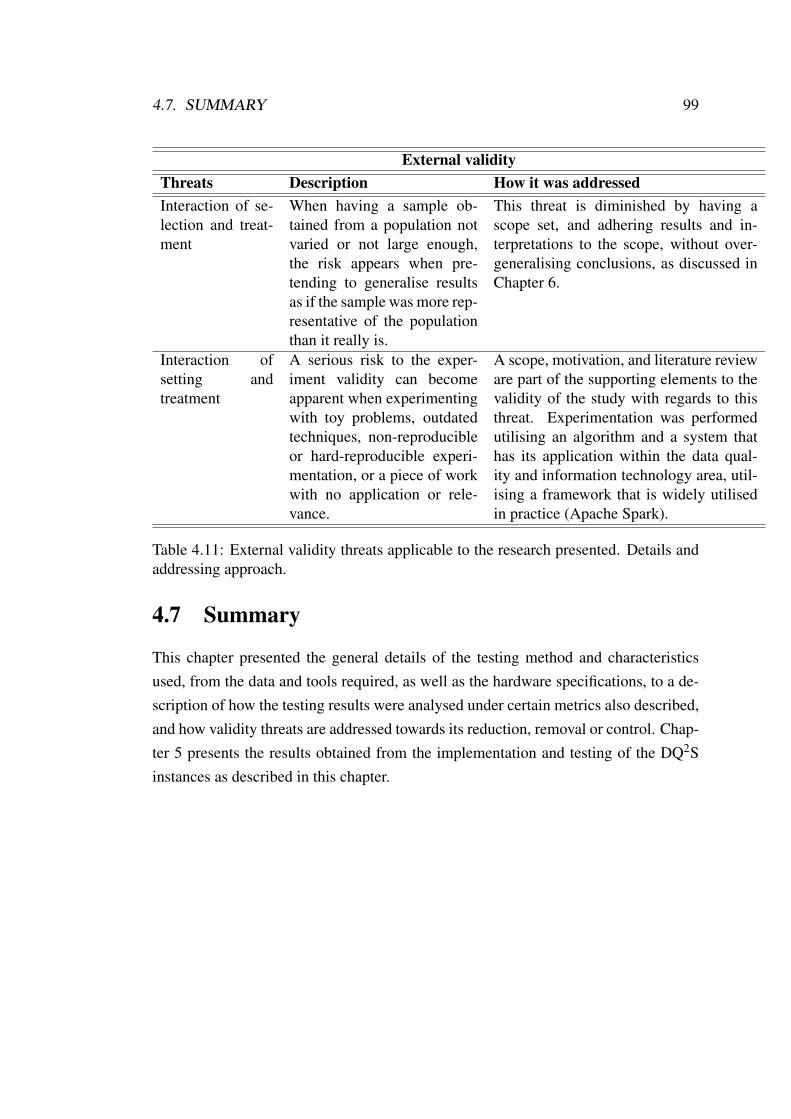
4.7. SUMMARY 99
External validityThreats Description How it was addressedInteraction of se-lection and treat-ment
When having a sample ob-tained from a population notvaried or not large enough,the risk appears when pre-tending to generalise resultsas if the sample was more rep-resentative of the populationthan it really is.
This threat is diminished by having ascope set, and adhering results and in-terpretations to the scope, without over-generalising conclusions, as discussed inChapter 6.
Interaction ofsetting andtreatment
A serious risk to the exper-iment validity can becomeapparent when experimentingwith toy problems, outdatedtechniques, non-reproducibleor hard-reproducible experi-mentation, or a piece of workwith no application or rele-vance.
A scope, motivation, and literature revieware part of the supporting elements to thevalidity of the study with regards to thisthreat. Experimentation was performedutilising an algorithm and a system thathas its application within the data qual-ity and information technology area, util-ising a framework that is widely utilisedin practice (Apache Spark).
Table 4.11: External validity threats applicable to the research presented. Details andaddressing approach.
4.7 Summary
This chapter presented the general details of the testing method and characteristicsused, from the data and tools required, as well as the hardware specifications, to a de-scription of how the testing results were analysed under certain metrics also described,and how validity threats are addressed towards its reduction, removal or control. Chap-ter 5 presents the results obtained from the implementation and testing of the DQ2Sinstances as described in this chapter.

Chapter 5
Evaluation of Experimental Results
Although performance can take into account more parameters than only executiontime, such as memory usage, energy consumption, and implementation cost [73], oneof the most important motivations for parallelisation is to get results within the mini-mum time possible [104, 3, 114, 123], thus, the experiments for this study were framedto rely on execution time, with few parameters aimed at developing a concise result set.
This chapter shows the results and analysis obtained from executing the set ofexperiments described in Section 4.4, utilising the average runtimes obtained fromfive executions of each query, and presents a discussion formed by the comparisonsdescribed in Section 4.5. The explicit values of the results are shown in Appendix C,where Section C.1 shows the raw results, and Section C.2 presents the performancemetrics calculated, both sections show results with a nine decimal precision.
5.1 Experiments Results
This section presents the results obtained from the execution of the experiments re-garding performance and scalability. The values shown are the averages obtained fromthe raw results shown in Appendix C, Section C.1. The results are presented in sub-sections aligned to the descriptions of the experiments shown in Section 4.4. After thefirst part of the results presented, comparison’s discussions are shown according to theorganisation and description made in Section 4.5.
100

5.1. EXPERIMENTS RESULTS 101
R1. E1 - Original Java DQ2S experiment - PC
Figure 5.1: Runtime registered in seconds for the Original Java DQ2S processing50 000, 100 000 and 1 000 000 rows.
The Original Java DQ2S implementation took around 7 minutes to process theTimeliness query (described in Chapter 3, Section 3.1.2) when utilising datasetsof 50 000 rows, 26 minutes with 100 000 rows datasets and 45 hours to runwith 1 000 000 rows datasets in the input dataset, as illustrated in Figure 5.1.These results were consistent with the experimental results presented at DQ2S’original publication, Sampaio et. al. [26], where the runtime of the Timelinessquery for an input of 100 000 rows was 56 minutes in a machine with half theamount of memory and CPU speed of the machine used in this research (desktop- PC machine described in Section 4.2). With the results obtained, the OriginalJava DQ2S is presented as not a suitable implementation to handle more than50 000 rows because of the relatively high runtime, considering that the sizein bytes for 1 000 000 rows is 84.5MB for the OrderT dataset and 68.9MBfor the statusTimelinessQR dataset. Based on these results, it is estimated thatthe original DQ2S implementation would need more than 40 hours to processthose 154MB with the Timeliness query. The reason why this Java instance isexpensive is mainly because of the Join operations required to execute this query,where each dataset has to be fully ingested first to be saved on its own array.Moreover, the OrderT dataset is scanned row by row to separate the pendingorders, and both datasets need to be joined with a method called addAll (asdescribed in Section 3.2.1), which generates a copy of the data. Lastly, another

102 CHAPTER 5. EVALUATION OF EXPERIMENTAL RESULTS
join operation adds the timeliness score to the former joined data. All thoserequirements cause the instance to spend a lot of time performing a sequentialscan and copying each of the rows.
R2. E2 - Python DQ2S experiment - PC
Figure 5.2: Runtime registered in seconds for the Python DQ2S processing 50 000,100 000 and 1 000 000 rows.
The Python DQ2S instance presented high runtimes, with 76 minutes to com-plete the Timeliness query when having datasets of 50 000 rows, 5 hours fordatasets of 100 000 rows and an average of 22 days to finish when processing1 000 000 rows. Runtime of the order of days is not efficient for data man-agement tasks, specially when handling relatively small data requires such longruntimes. Such behaviour places the Python DQ2S to be a non-suitable option toprovide DQ2S the capability of handling big data.
Python is often considered an interpreted language, however, it is not a purelyinterpreted one [35, 80]. Python combines interpreting and compiling char-acteristics. A Python program is implicitly compiled on its execution to bytecode, which is later interpreted. Regarding performance, Python is known to runslower than low level languages such as C or C++. This is because some piecesof code from Python are not fully compiled, and thus, require more executiontime to be interpreted by the machine. The above represents one of the reasonswhy the Python DQ2S presented high runtimes, as well as the fact that Pythonis dynamically typed, which causes the Python interpreter to spend time inspect-ing each object to identify its data type to call the appropriate routines. Anotherdrawback is Python’s object model that causes inefficient memory access due to

5.1. EXPERIMENTS RESULTS 103
segmentation, compared to the object model of Python’s scientific libraries suchas NumPy and Pandas [141, 142] which allow contiguous memory allocation.
R3. E3 - Optimised Python DQ2S experiment - PC
Figure 5.3: Runtime registered in seconds for the Optimised Python DQ2S processing50 000, 100 000 and 1 000 000 rows.
The Optimised Python DQ2S presented significantly better results, with runtimesof less than one second for the Timeliness query when processing 50 000 and100 000 rows, and less than two seconds for the 1 000 000 rows dataset, as shownin Figure 5.3. The scalability of this implementation can be considered goodtaking into account that less than two seconds for the larger workload presentedin the experiments is an acceptable runtime to work with when utilising DQ2Sinstead of runtime of hours or even days. However these results appear as abaseline upon which further exploration is required, considering that 1 000 000rows is not as large a data set according to current trends can be. Even thoughDQ2S needs to be able to cope with larger volumes of data, the Optimised Pythoninstance seems to be a promising support for bigger workloads with such smallruntimes. Results of Experiment 4, shown in R4 below, present an analysis onthe Optimised Python DQ2S for larger datasets.
As described in Section 3.2.3, this DQ2S instance was developed utilising aPython Data Analysis library called “Pandas”. The use of this library reducesthe work of the Timeliness query allowing a more straight-forward and opti-mised usage of functionalities common to tabular data, offered by the library.A summary of the specific differences regarding code and how it decreases the

104 CHAPTER 5. EVALUATION OF EXPERIMENTAL RESULTS
cost of some operations, such as eliminating the need for copying row by rowwith custom code to perform a join operation, is shown in Section 3.2.3, Table3.4 where the table presents a relation on the main differences that the usage ofa Python scientific library imply. The results of the experiment presented in thissubsection (Experiment 3) shows that those simple code optimisations have animpact on the runtime.
R4. E4 - Optimised Python DQ2S maximum capacity experiment - PC
Dataset size(rows)
Dataset size Result DetailsOrderT statusTimelinessQR
5 000 000 444.5MB 348.9MB OK ∼9 secs
10 000 000 894.5MB 689.5MB OK ∼18 secs
15 000 000 1.4GB 1.1GB FAIL Error tokenizing data.
C error: out of memory.
Segmentation fault (core
dumped)
14 000 000 1.3GB 982.9MB FAIL
13 000 000 1.2GB 911.9MB FAIL
12 000 000 1.1GB 840.9MB FAIL
11 000 000 989.5MB 769.9MB OK ∼20 secs
11 500 000 1GB 805.4MB OK 21.34 secs
Table 5.1: Relation of the dataset sizes and results when executing Optimised PythonDQ2S in a single machine for Experiment 4.
Dataset size(rows)
Dataset size
OrderT statusTimelinessQR
12 000 000 1 084 457 625 bytes 840 891 569 bytes
11 500 000 1 036 957 625 bytes 805 391 569 bytes
Table 5.2: Size in bytes for the first dataset that caused a failure (12 000 000 rows), andthe maximum number of rows processed by the Optimised Python DQ2S (11 500 000).
The Optimised Python DQ2S cannot be considered as a suitable option for bigdata processing solely based on runtime results when handling relatively smallvolumes of data, as shown in the results of Experiment 3 (R3 above). To evalu-ate the suitability of the Optimised Python implementation for processing largerdatasets it is necessary to know how much data it can handle, for which thisexperiment was designed.

5.1. EXPERIMENTS RESULTS 105
Following the procedure described in Section 4.4 for Experiment E4, 11 500 000rows appeared as the maximum size this Optimised Python DQ2S instance couldprocess successfully, with a runtime of 21.34 seconds. The experiment, as pre-sented in Table 5.1, showed an out of memory failure for the datasets larger than11 500 000 rows, where 12 000 000 rows is the first dataset size that caused afailed processing. The failure appeared under the Pandas I/O API reader func-tion called read csv, which aims at reading data from a CSV format to convertit into a dataFrame object [29]; currently this is the most efficient way to ingestdata from an outer file in Python programming, compared to the implementa-tion that could be done from scratch. The Pandas reader functions are set toload data without further programming specifications but only certain parame-ters, such as specifying the token delimiter, date time and error handling options,data types inference or manually set, etc., which otherwise should be coded ex-plicitly, likely involving more implementation effort and higher error rates.
The difference between the last input data size that was successfully processed,and the first that was not, as shown in Table 5.2 is 47 500 000 bytes (1 084 457 625- 1 036 957 625) for the OrderT dataset, and 35 500 000 bytes (840 891 569 -805 391 596) for the statusTimelinessQR dataset, this is, in sum, a differenceof ∼79MB which made a separation between success and failure for the queryprocessing. The maximum input that the Optimised Python DQ2S could copewith, according to the results shown in this subsection, has a size of few bytesless than 2GB, this is the limit in which the technique utilised with the OptimisedPython DQ2S instance is no longer enough for the desktop machine utilised inthis study. The out of memory failure shown in Table 5.1 is presented when thequery process required more memory than the available allocated to the Pan-das CSV reader, hence if more main memory was available (e.g. a machine withmore than 16GB of RAM) this limit could be increased, however, without addingresources, there is a possibility to increase this limit by implementing a functionto read input datasets iteratively in chunks, which would increase the limit to over11 500 000 rows (∼2GB), according to performed experiments which results areshown in Table 5.1. However, this solution causes an increase in runtime becauseof the I/O process done in iterations in this case. The cost of each round wouldprobably depend on the number of rows consumed per iteration (these are calledchunks), as well as the content of the chunk. The exploration of workarounds toovercome this limitation is out of scope for this study.

106 CHAPTER 5. EVALUATION OF EXPERIMENTAL RESULTS
Although the Optimised Python DQ2S offered good performance processing11 500 000 rows in 21.34 seconds, the available Python programming librarydoes not offer a memory-efficient ingestion approach by itself [111], and even ifan amendment is made, the instance would still be a sequential implementationof the algorithm that comprises I/O traditional processes, loading data from diskto main memory and back, thus, when reaching the point in which data couldnot longer fit into memory, the program will not be usable for processing [87].
To summarise, the important aspects of the results gathered in this experimentare as follows:
• 11 500 000 rows is the maximum dataset size that the Optimised PythonDQ2S could cope with in the desktop machine (PC) utilised in the experi-mentation.
• The difference between 11 5000 000 rows and the first dataset size thatcaused a failure is ∼79MB.
• Above 11 500 000 rows, a failure caused by the Pandas data reader, themost efficient ingestion function for Python language, presents an out ofmemory error because the program tries to utilise more memory than theone that is allocated for its process.
• The failure could be amended by creating a segmentation of the data, insuch a way the reader can load chunks of data instead of trying to readthe whole data at once, creating a reading and loading iterative process.This can be related to the MapReduce and big data processing paradigmsof utilising data segmentation and lazy data evaluations.
R5. E5 - PySpark DQ2S Standalone mode in single machine experiment - PC
The PySpark DQ2S executed using a Standalone deployment in a single desk-top machine, presented its best results when configured to run with 1 workerand 4 cores (1W4C), this is, 1 executor running on the machine, handling 4tasks simultaneously (refer to Section 3.2.4 for Spark definition of its compo-nents). This was true for all of the three different dataset sizes, as shown in Fig-ure 5.4, where the quickest runtime with 1W4C configuration was 7.38 secondsfor 50 000 rows, 7.64 seconds for 100 000 00 rows, 11.77 seconds for 1 000 000rows. With regards to scalability, the PySpark DQ2S execution without paralleli-sation (this is, 1 worker and 1 Core), the execution runtime increased 1.05 times

5.1. EXPERIMENTS RESULTS 107
when the input datasets were increased from 50 000 rows to 100 000 rows, andthe runtime was doubled when the input dataset was increased 10 times, in num-ber of rows (from 50 000 rows to 1 000 000). The scalability rates presented with1W1C configuration suggest it might be easy for this implementation to reacha point in which runtime is not longer acceptable for much larger dataset sizes,because the runtime increases at a high rate when the data volume increases too.However, for runtimes obtained with 1W4C configuration, when doubling thedata the execution time rate increased 1.03 times, and 1.5 times when having1 000 000 rows, which is a more acceptable rate considering it is below dou-bling the runtime, and below the rates that the sequential configuration (1W1C)presented.
Figure 5.4: Runtime registered in seconds for the PySpark DQ2S processing 50 000,100 000 and 1 000 000 rows in Standalone mode implemented in a single machine,where W refers to workers and C to cores in the Apache Spark definition. The markedline indicates the lower runtime obtained per dataset size.
For the three different dataset sizes (50 000, 1 000 000, and 1 000 000 rows),and the experiment configured to 1 worker (with 1 Executor each), the runtimeand the runtime difference between configurations, decreased when adding morecores to the configuration. Table 5.3 shows the relation of the decreasing run-time when adding more cores to 1 worker for datasets of 50 000, 100 000 and1 000 000 rows, where results show scalability more clearly when larger datasetsare processed, this is because when processing larger data sets, runtime is dom-inated by data processing related tasks, rather than system set up tasks. This

108 CHAPTER 5. EVALUATION OF EXPERIMENTAL RESULTS
behaviour can probably explain the reason why the results obtained from exper-iments where configurations with more than one worker was used showed that,when the number of workers was set to 2 there was a runtime decrease betweena configuration with 1 Core (2W1C) and 2 cores (2W2C), but the runtimes werestill higher than the ones obtained with 1 worker (1W1C, 1W2C, 1W3C and,1W4C). Another observation related to this behaviour was made when adding3 and 4 workers, with 1 core allocated per worker (3W1C and 4W4C), wherethe runtimes were higher than the configurations with 1 and 2 workers, exceptfor the larger datasets. For executions with 50 000 and 100 000, the worst run-time was obtained from the configuration with 4 workers and 1 core (4W1C).However, for 1 000 000 rows, the 4W1C configuration did not incur the highestruntime. The obtained runtime being not as good as the best runtime from exe-cutions with 1W4C configurations seem to suggest that the best configuration forexecuting a job should be decided based on the amount of work needed by theapplication and the dataset size, requiring a debug and fine tuning work to findthe optimum configuration depending on the processing intensity of the Sparkapplication given by the operators needed, or the dataset sizes within a certainuse case. Even though Spark runs in a single machine in this experiment, it canbe noticed that Spark able to offer the benefits that can be obtained from paral-lelism, tackling runtime and memory management, as well as scalability, withan added advantage of not requiring explicit parallelism to obtain such benefits.
Seconds decreasedNumber of rows
Configuration50 000 100 000 1 000 000
Seconds decreased fromruntime with one more core
&Seconds decreasedfrom base runtime
10.57 11.20 20.77Base runtime (seconds):
1W1C2.29 2.48 6.28 1W2C0.51
&
2.8
0.79
&
3.27
2.11
&
8.39
1W3C
0.39
&
3.19
0.29
&
3.56
0.61
&
9
1W4C
Table 5.3: Relation of seconds decreased from different configurations using 1 worker(W) and 1 to 4 cores (C) with the Standalone mode in a single machine.

5.1. EXPERIMENTS RESULTS 109
R6. E6 - PySpark DQ2S Local mode in single machine experiment - PC
Figure 5.5: Runtime registered in seconds for the PySpark DQ2S processing 50 000,100 000 and 1 000 000 rows in Local mode implemented in a single machine. Themarked line indicates the lower runtime obtained per dataset size.
Figure 5.6: Runtime registered in seconds for the PySpark DQ2S processing 50 000rows in Local mode implemented in a single machine.

110 CHAPTER 5. EVALUATION OF EXPERIMENTAL RESULTS
Figure 5.7: Runtime registered in seconds for the PySpark DQ2S processing 100 000rows in Local mode implemented in a single machine.
Figure 5.8: Runtime registered in seconds for the PySpark DQ2S processing 1 000 000rows in Local mode implemented in a single machine.

5.1. EXPERIMENTS RESULTS 111
Times Slower: PySpark local[1]vs PySpark local[8]
Dataset Size(rows)
Runtime (seconds) Times Slower
PySpark
local[1]
PySpark
local[8]local[1]<local[8]
50 000 6.92 4.62 1.49
100 000 7.59 4.99 1.51
1 000 000 17.69 9.37 1.88
Table 5.4: Times Slower: Relation between the runtime results of the PySpark instancewith 1 (sequential) and 8 threads (best time). Where local[1]<local[8] indicates thePySpark DQ2S in local mode with 8 threads is slower than the same implementationwith 8 threads as many times as indicated.
Without any change to the PySpark code, but setting the Spark master to a Localmode (refer to Section 4.3.1 for details of the Local mode concepts) the execu-tion times were below 10 seconds for 50 000 and 100 000 rows, and below 20seconds for 1 000 000 rows. The best runtime obtained from the 50 000 and100 000 rows dataset was obtained when setting 8 threads, with 4.62 secondsfor 50 000 rows, and 4.99 seconds for 100 000 rows, whereas for the biggestdataset size in this experiment, the best runtime was 8.73 seconds, obtained with7 threads, as shown in Figure 5.5. The runtimes obtained decreased by mil-liseconds as more threads were added to the configuration each time, having thebiggest observable reduction in Figure 5.5 for the set of 1 000 000 rows, wherealmost 6 seconds were reduced from a sequential execution (this is, when usinglocal[1]) to 2 threads.
The ratio of how much slower is the sequential configuration (local[1]), com-pared to the one that offered the best performance in runtime terms (the configu-ration with local[8]), was around 1.5 and 1.9, as shown in Table 5.4, these resultssuggest that it is possible to reduce the runtime by almost half by adjusting theparametrisation. In terms of scalability, for the sequential configuration, which isthe one set with 1 thread, the 100 000 rows execution offered 1.09 times slowerresults in seconds compared to the runtime presented by half of the dataset size,and 2.5 times slower for 1 000 000 rows compared to the times obtained with50 000 rows. For the times gathered with 8 threads, the scalability results are1.08 times slower for twice of the data volume from the smaller dataset size,

112 CHAPTER 5. EVALUATION OF EXPERIMENTAL RESULTS
and 2.02 times slower for 1 000 000 rows. There appears to be not much differ-ence on the scalability offered by either 1 or 8 threads when the data is relativelysmall (e.g. for the 50 000 rows datasets processing), and neither the runtimesare hugely different with distinct number of threads. It seems to be the case thatSpark implemented in Local mode presents parallelism, but the execution of thewhole processes on the same JVM causes Spark to utilise all of the resourcesavailable for one JVM, lacking a spawn of resources among processes. This re-sources spawning cannot happen because of the Local mode configuration thatprocesses everything on the same JVM, thus, utilising the same configurationwith few differences, the opposite to a Standalone mode where different config-urations cause more impact on the internal Spark set-up. (refer to Section 4.3for more details of the Standalone mode) This is why there are not hugely differ-ences when setting more threads to be handled in Local mode. Figure 5.6, 5.7,and 5.8 show the runtimes registered for each of the datasets utilised in this ex-periment, where it is observable that the biggest runtime decrease is made whenchanging from processing one thread to divide the tasks in two threads.
R7. E7 - PySpark DQ2S Local mode maximum capacity experiment - PC
Figure 5.9: Runtime registered in seconds for the PySpark DQ2S processing11 500 000 and 35 000 000 rows in Local mode implemented in a single machine.The marked line indicates the lower runtime obtained per dataset size.

5.1. EXPERIMENTS RESULTS 113
Figure 5.10: Runtime registered in seconds for the PySpark DQ2S processing11 500 000 rows in Local mode implemented in a single machine.
Figure 5.11: Runtime registered in seconds for the PySpark DQ2S processing35 000 000 rows in Local mode implemented in a single machine.
This experiment aimed at discovering the limitations of the Apache Spark Lo-cal mode implementation, by searching for the maximum data size that couldbe handled successfully utilising the dekstop machine (PC). This experimentfollowed the procedure described in Section 4.4, Experiment E7, where it wasobtained a successful result for up to 35 000 000 rows. When trying to pro-cess datasets with more than 35 000 000 rows, a java.lang.NegativeArray
SizeException with CsvRelation error was produced when the show action

114 CHAPTER 5. EVALUATION OF EXPERIMENTAL RESULTS
in the PySpark code triggered the whole processing of the Timeliness query. Ex-ecutions of the Timeliness query for input data sets with more than 35 000 000rows, or 3.3GB for the orderT dataset and 2.5GB for the statusTimelinessQR
dataset, failed. The error might appear to be related to a difference in sizes withthe schema inferred by PySpark and the rows information, or because of a faultydataset with missing data, but it is important to revise the complete error logbecause there are multiple different types of error associated with the NegativeArray Size Exception in Spark, making the finding of a diagnosis of the error adifficult task. For example, this error could be caused by any of the following:(i) because the buffer used to store more data than it is allowed to keep, there-fore, unable to fit all of the data required, (ii) because of the serialization issuewhich affects the Python socket (called py4j; refer to Section 3.2.4 for details ofpy4j socket) when dealing with strings larger than 2GB, (iii) because an integeroverflow caused by an array handling large messages, or (iv) because of largeprocess within the code, which is the case of an error that can be produced whenjoining. The reason of the failure with large datasets in this case is the number(iv). The error could possibly be identified by debugging the log displayed byPySpark, but the task of diagnosing the error from the log would still be a chal-lenging one, because Spark-generated error lots present significant similarities[65, 64, 21, 79, 78]. Being a relatively new technology, the causes of run timeexceptions are not always clear, and in the majority of cases, an exception couldbe raised by an implementation error by a programmer, or because some resourcehas exhausted. More than 1500 issues of that nature have been documented asunresolved, with new issues coming each month [63]. While workarounds aresuggested by the Spark community, work is still needed. Further research aboutSpark’s general usability for common processes, as well as the implementationof amendments to the default functions, are out of the scope of this study.
This experiment comprised the configuration of more cores than the numberof CPU cores available on the machine. The hypothesis to be tested was thatfixing a maximum number of cores equal to the maximum available CPU coresoffers the best runtime compared to any other number of cores configured. Theperformed tests used from 1 to 10 cores, 12 and 16 cores to investigate whatis the impact of increasing the number of cores on relation to the number ofavailable CPU cores [47, 39]. Results for the PySpark DQ2S support the practiceof aligning number of cores to the number of CPU cores available, based on the

5.1. EXPERIMENTS RESULTS 115
fact that the best runtime was produced when the number of cores was set to8, and for higher number of cores, the runtime began to be higher, as shown inFigure 5.9. Figures 5.10 and 5.11, show the results in separate obtained for theprocessing of 11 500 000 and 35 000 000 rows, where it can be observed thatas more threads are added (refer to Section 4.3.1 for details of the correlationbetween cores and threads), the execution runtime shows a very similar curveeither with the 11 500 000 rows datasets or the datasets of 35 000 000 rows,which suggests the data volume does not change the impact of the number ofcores configured, this is, for any size, the number of cores configured should bethe number of CPU cores available.
R8. E8 - PySpark DQ2S cluster Standalone mode experiment - Cluster
Dataset size(rows)
Dataset size
OrderT statusTimelinessQR
35 000 000 3.3GB 2.5GB
70 000 000 6.6GB 5GB
105 000 000 9.9GB 7.4GB
Table 5.5: Size in GB for the datasets sizes processed on the cluster.
Figure 5.12: Runtime registered in seconds for the processing of 35 000 000,70 000 000, and 105 000 000 rows with PySpark DQ2S in Standalone mode usedin a cluster, utilising from 1 to 4 nodes (worker nodes). Each node was configured tocontain 1 worker process with 8 executors, each executor with 2 cores and 32GB ofavailable memory.

116 CHAPTER 5. EVALUATION OF EXPERIMENTAL RESULTS
This experiment is the first set of tests performed in the cluster (DPSF) (de-scribed in Section 4.2). The execution was done with a Standalone deploymentof Apache Spark, following the procedure described for Experiment 8 in Section4.4. The smaller input datasets processed in this experiment have 35 000 000rows, based on the maximum size successfully handled by the PySpark in a sin-gle machine, under the Local mode. The results from experiments performed us-ing Spark on Local mode, namely Experiment 7 (R7 in this section), are utilisedas reference to set the initial dataset size used for this experiment, rather thanthe results from Spark on Standalone mode showed in Experiment 5 (R5 inthis section), as the reader would probably expect, because, unlike the Sparkon Standalone mode running on a single machine, the Local mode allows a sin-gle machine to utilise Spark’s capabilities without trading on performance dueto the limitation of not having a cluster, as discussed in Section 4.3.1. To repre-sent an intermediate workload in this experiment, input data sets of 70 000 000rows were chosen, doubling the size of the input data sets used in the start-ing workload. Finally, when tripling the starting dataset sizes, input datasets of105 000 000 rows represent the larger workload in this experiment. The relationof number of rows and the size in GB is shown in Table 5.5.
The best runtime results for the three input data sizes described above were ob-tained when 4 worker nodes were used in the execution of the Timeliness queryover the DPSF cluster, as Figure 5.12 shows. Note from the figure the runtimesobtained for executions of sets with 35 000 000 rows was done in few moreseconds than a minute when utilising one node (71.62 seconds), and less thanhalf a minute with 4 nodes (28.65 seconds). The medium workload requiredfew less than two minutes when processed with one node (115.20 seconds), andstill less than a minute using 4 nodes (46.01). The larger dataset utilised, tookfew more than 2 minutes as runtime with the Timeliness query processed in onenode (145.85 seconds), and less than a minute when using 4 nodes (58.61 sec-onds). This confirms that, for executions on a cluster infrastructure, Spark inStandalone mode supports a DQ2S implementation producing acceptable pro-cessing capabilities on large datasets, considering that few minutes is a fair timefor handling millions of rows; results also show scaling-out techniques behavewell with Spark, offering parallelism reflected on quicker results each time anode is added, where each node is not adding more resources to the process byhaving larger capabilities (scale-up) but by adding more resources with the usage

5.1. EXPERIMENTS RESULTS 117
of more nodes (scale-out).
The quick runtimes reflected on the results might be possibly achieved due toSpark’s abstraction to a parallel collection model, known as RDD (refer to Sec-tion 2.3.1 for details of RDDs), which partitions the data across nodes, and sup-ports reutilisation without requiring data to be replicated [151], providing CPUintense applications, rather than I/O heavy load [100], which causes Spark ap-plications to occupy main memory and CPU capabilities on an higher utilisationthan the required interaction with storage.
R9. E9 - Optimised Python DQ2S cluster experiment - Cluster
Dataset size(rows)
Dataset size Result DetailsOrderT statusTimelinessQR
35 000 000 3.3GB 2.5GB OK 83.22 secs
40 000 000 3.7GB 2.8GB OK ∼112 secs
50 000 000 4.7GB 3.5GB FAIL Error tokenizing data.
C error: out of memory.
Segmentation fault (core
dumped)
70 000 000 6.6GB 5GB FAIL
105 000 000 9.9GB 7.4GB FAIL
Table 5.6: Relation of the dataset sizes and results when executing the OptimisedPython DQ2S in the cluster for Experiment 9.
Running any large job on a cluster is always better than running the same jobon a (single) commodity machine, having a big data platform available fromthe cluster or not. However, without the platform, the parallelism exploitationhas to be encode within the job. The Optimised Python DQ2S was executed inthe DPSF cluster, providing a view of the performance that can be obtained forDQ2S without a big data framework. The Optimised Python version was in-tended to be tested in a cluster environment aiming at getting comparable resultsto the ones obtained with the PySpark DQ2S instance on a sequential configu-ration in a cluster environment, were both implementations would use only onenode, hence, the same dataset sizes were tried (35 000 000, 70 000 000 and105 000 000 rows). Results were successful only for the dataset with 35 000 000rows, with a runtime of 83.22 seconds, as shown in Table 5.6. Larger datasets

118 CHAPTER 5. EVALUATION OF EXPERIMENTAL RESULTS
produced an out of memory failure, also obtained in Experiment 4 (R4 in thischapter), caused by insufficient memory space for the execution of the job.
To explore the limits of the instance on the DPSF cluster, a 40 000 000 rows inputdatasets were processed with success taking around 112 seconds, and 50 000 000rows, or 8GB of total input was the first size tested that produced a failure.The execution of this instance utilised a single node on the DPSF cluster, with512GB of main memory, a much higher capacity compared to the input of 8GB.The limits on memory and the failure that appeared is dependent on the memoryavailable for the Python process, specifically for the stack allocated by the OS,therefore, this limit is also dependant on RAM and OS, which explains the reasonof a bigger limit for the Optimised Python on a cluster, compared to the limit of2GB obtained in a desktop machine.
5.2 Algorithm Comparison
This section presents insights obtained from analysing the results shown in Sec-tion 5.1. Appendix C, Section C.2, shows the raw results obtained for the calcu-lation of the performance metrics.
R10. C1 - The original DQ2S Java program (E1) compared with its equivalentDQ2S developed using Python (E2).
Times Slower: Original Java vs Python
Dataset Size(rows)
Runtime (seconds) Times Slower
Java Python Python <Java
50 000 397.59 4612.62 11.6
100 000 1593.84 19019.20 11.9
1 000 000 160624.02 1974593.50 12.4
Table 5.7: Times Slower: Relation between Original Java and Python runtime results.Where Python <Java indicates the Python DQ2S is slower than the Java implementa-tion as many times as indicated.
The results from the original DQ2S Java program (R1 in this section) and its

5.2. ALGORITHM COMPARISON 119
equivalent algorithm implemented in Python language (R2 in this section), pre-sented different runtimes, where the Java program was apparently 11 to 12 timesfaster than the Python version, as shown in Table 5.7. There are several bench-marking studies and discussion which of Java or Python is faster [141, 85, 149,94, 108, 153, 135]. Most of the studies present Python as more computationallyexpensive than Java, but they all agree that it is naive to state that a program-ming language is more efficient than another for all cases and situations, sincethe runtimes depend on several parameters, such as optimization level, the algo-rithm complexity, the verbosity of the code, the compiler utilised, and even thehardware involved.
For both the Python and Java DQ2S implementations runtime quadrupled wheninput data sizes were increased from from 50 000 to 100 000 rows, and ∼100times when increasing the dataset size to 1 000 000 rows. These rates show bothinstances present a similar scalability pattern but the Java version offers betterperformance, which is consistent with the common view of Java being fasterthan Python, due to the static nature of Java and the fact that it is a compiledlanguage rather than interpreted. Python has the option to run over differenttypes of compilers, such as Jython, Skulpt, IronPython, ActivePython, amongothers, which could offer different results, and provide a research area towardspossibly leveraging performance of DQ2S on pure Python code, nevertheless,this research aims at other objectives focused on big data frameworks.
R11. C2 - The Python DQ2S program (E2) compared with the Optimised Pythonversion of it (E3).
The results of the sequential Python DQ2S, presented in R2 of this section, andthe Optimised Python version (also sequential) depicted in R3, show a significantdifference between the obtained runtimes:
The non-optimised Python implementation of DQ2S incurs, as expected, longerruntimes compared to the Optimised implementation. The Optimised PythonDQ2S presented better scalability results than the Python DQ2S. this can be in-terpreted considering that the Optimised Python DQ2S required 1.7 times moreseconds when the data volume was doubled from 50 000 rows to 100 000 rows,and 9.4 times more seconds when increasing the dataset size from 100 000 rowsto 1 000 000, whereas the Python DQ2S required 4.1 and 103.8 times more sec-onds respectively. Those results can be interpreted as providing better scalability
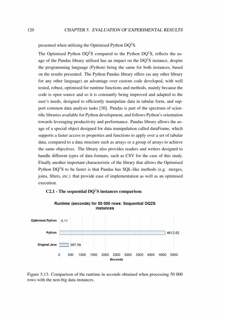
120 CHAPTER 5. EVALUATION OF EXPERIMENTAL RESULTS
presented when utilising the Optimised Python DQ2S.
The Optimised Python DQ2S compared to the Python DQ2S, reflects the us-age of the Pandas library utilised has an impact on the DQ2S instance, despitethe programming language (Python) being the same for both instances, basedon the results presented. The Python Pandas library offers (as any other libraryfor any other language) an advantage over custom code developed, with welltested, robust, optimised for runtime functions and methods, mainly because thecode is open source and so it is constantly being improved and adapted to theuser’s needs, designed to efficiently manipulate data in tabular form, and sup-port common data analysis tasks [30]. Pandas is part of the spectrum of scien-tific libraries available for Python development, and follows Python’s orientationtowards leveraging productivity and performance. Pandas library allows the us-age of a special object designed for data manipulation called dataFrame, whichsupports a faster access to properties and functions to apply over a set of tabulardata, compared to a data structure such as arrays or a group of arrays to achievethe same objectives. The library also provides readers and writers designed tohandle different types of data formats, such as CSV for the case of this study.Finally another important characteristic of the library that allows the OptimisedPython DQ2S to be faster is that Pandas has SQL-like methods (e.g. merges,joins, filters, etc.) that provide ease of implementation as well as an optimisedexecution.
C2.1 - The sequential DQ2S instances comparison
Figure 5.13: Comparison of the runtime in seconds obtained when processing 50 000rows with the non-big data instances.
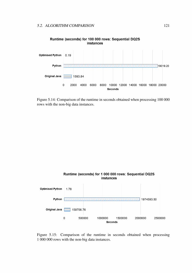
5.2. ALGORITHM COMPARISON 121
Figure 5.14: Comparison of the runtime in seconds obtained when processing 100 000rows with the non-big data instances.
Figure 5.15: Comparison of the runtime in seconds obtained when processing1 000 000 rows with the non-big data instances.

122 CHAPTER 5. EVALUATION OF EXPERIMENTAL RESULTS
Times Slower: Python vs Optimised Python
Dataset Size(rows)
Runtime (seconds) Times Slower
PythonOptimised
PythonPython <Optimised Python
50 000 4612.6 0.1 43478.1
100 000 19019.2 0.2 99758.1
1 000 000 1974593.5 1.8 1107362.4
Table 5.8: Times Slower: Relation between Python and Optimised Python runtimeresults. Where Python <Optimised Python indicates the Python DQ2S is slower thanthe Optimised Python implementation as many times as indicated.
Times Slower: Original Java vs Optimised Python
Dataset Size(rows)
Runtime (seconds) Times Slower
JavaOptimised
PythonJava <Optimised Python
50 000 397.59 0.11 3747.7
100 000 1593.84 0.19 8359.9
1 000 000 160624.02 1.78 89592.4
Table 5.9: Times Slower: Relation between Original Java and Optimised Python run-time results. Where Java <Optimised Python indicates the Java DQ2S is slower thanthe Optimised Python implementation as many times as indicated.
At this point in the analysis, the results make it possible to select the best sequen-tial instance to be used as baseline with evidence. In the following, a summaryof the results presented in R1, R2, R3, R10 and R11 of this chapter is provided.
The original Java DQ2S instance was faster than the Python version. These twoinstances were developed without usage of any specialised library (such as Pan-das), and utilised the original structure of the DQ2S set of algorithms, describedin Section 3.1.4. Whereas the Optimised Python version is implemented withheavy use of a scientific tabular data manipulation library. Figures 5.13, 5.14,and 5.15 provide a visual comparison of the three sequential, non-big data DQ2Sinstances (Original Java, Python and Optimised Python) for each of the basicdatasets (50 000, 100 000 and 1 000 000 rows). The presentation of these results

5.2. ALGORITHM COMPARISON 123
are made in separated graphs to ease the comparison due to the different scalesthat each set of results comprises. Regarding runtime, the Optimised Python,presents the best results by being at least 3 700 times faster than the Java and thePython DQ2S. Tables 5.8 and 5.9 present the relation of times slower of the Javaand Python sequential instances in comparison to the Optimised Python DQ2S.
R12. C3 - The Optimised DQ2S Python program (E3) compared with the PyS-park program in Local mode (E6).
Figure 5.16: Comparison of the runtime in seconds obtained when processing 50 000,100 000 and 1 000 000 rows with the best non-big data instance (sequential) and itsimplementation with a big data instance using 1 and 8 threads .

124 CHAPTER 5. EVALUATION OF EXPERIMENTAL RESULTS
Times Slower: Optimised Python vs PySpark local[1]
DatasetSize (rows)
Runtime (seconds) Times Slower
OptimisedPython
PySparklocal[1]
local[1] <Optimised Python
50 000 0.11 6.92 65.2
100 000 0.19 7.59 39.8
1 000 000 1.78 17.69 9.9
Table 5.10: Times Slower: Relation between the runtime results of the OptimisedPython and PySpark with 1 thread. Where local[1]<Optimised Python indicates thePySpark DQ2S in local mode with 1 thread is slower than the Optimised implementa-tion as many times as indicated.
Times Slower: Optimised Python vs PySpark local[8]
DatasetSize (rows)
Runtime (seconds) Times Slower
OptimisedPython
PySparklocal[8]
local[8] <Optimised Python
50 000 0.11 4.62 43.5
100 000 0.19 4.99 26.1
1 000 000 1.78 9.37 5.3
Table 5.11: Times Slower: Relation between the runtime results of the OptimisedPython and PySpark with 8 threads. Where local[8]<Optimised Python indicates thePySpark DQ2S in local mode with 8 threads is slower than the Optimised implemen-tation as many times as indicated.
This comparison includes the results obtained from the Optimised DQ2S Pythonprogram, which is a sequential implementation, and the results from the PySparkinstance, comprising the Spark execution without parallelism (local[1]), and thebest runtime obtained with 8 threads (local[8]). Spark applications, such as PyS-park DQ2S can run on a single machine with implicit parallelism, dividing thetasks and data to complete the job among several threads, and can also completea job as a sequential instance with a configuration that sets the PySpark DQ2S torun with one thread.

5.2. ALGORITHM COMPARISON 125
The aim of comparing the sequential results from the Optimised Python DQ2Sagainst the results obtained from executions of the PySpark implementation us-ing a single thread is to analyse the impact of the big data framework causedsolely by its usage, whereas, the aim of comparing the sequential results fromthe Optimised Python DQ2S against the PySpark DQ2S obtained with 8 threadsis to analyse the best results obtained, with the purpose of avoiding a disadvan-tage by default for PySpark by not considering the best capability offered byit.
The Optimised Python was quicker when processing each of the three datasetsizes tested, compared against both the PySpark results running with both oneand eight threads (local[1] and local[8]), as shown in Figure 5.16. Note thatthe PySpark instance was at least 5 times slower than the Optimised Python,as reflected in Tables 5.10 and 5.11. The runtime results could indicate thatthe Optimised Python instance is a better option for big data quality processingthan the PySpark implementation. However, in terms of scalability, the PyS-park instance presents a smaller gap when the dataset size is increased, and, ascommented in R4 and R6 of Section 5.1, scalability for the Optimised Pythonwhen increasing the volume of data 20 times (from 50 000 000 to 1 000 000rows) is 16 times more seconds whereas the scalability for the PySpark with 8threads is 1.87 times more seconds for the same case. An overhead is observedin the PySpark instance, that is not present in the Optimised Python program,this is to set up the application processes within the framework system, to ini-tiate the executor process and for the task scheduler to set the tasks, generatethe execution plan, allocate the resources, coordinate the results, and finally turndown the deployment. Runtime is the focus of parallel performance but it is notisolated from scalability, in practical terms, there is not much gain having thequickest algorithm if it is not capable of coping with big data. This is a worthytrade-off, seeking for a fair speed but great scalability, and in this sense, PySparkhas performed better than the Optimised Python, having both its default param-eters, with not much tuning involved, because effort and productivity could alsotake part when selecting the best technology and technique to process big data iftuning is involved.

126 CHAPTER 5. EVALUATION OF EXPERIMENTAL RESULTS
R13. C4 - The maximum number of rows processed by the Optimised DQ2SPython program (E4) compared with the PySpark program in Local mode(E7).
Figure 5.17: Comparison of the runtime in seconds obtained when processing11 500 000 rows with the best non-big data instance and the PySpark one with 1 and 8threads.
Times Slower: Optimised Python vs PySpark local[1] and local[8]
Dataset Size (rows) Runtime (seconds)
Optimised Python Optimised Python PySpark local[1] PySpark local[8]
11 500 000 21.35 132.28 43.71
Comparison Times slower
local[1] <Optimised Python 6.20
local[8] <Optimised Python 2.04
local[1]<local[8] 3.02
Table 5.12: Times Slower: Relation between the runtime results of the OptimisedPython and PySpark with 1 and 8 threads for 11 500 000 rows. Where the notationimplementation <implementation indicates the left implementation is slower than theimplementation on the right as many times as indicated.

5.2. ALGORITHM COMPARISON 127
Figure 5.18: Ideal Speedup compared against the speedup results obtained from thePySpark DQ2S Local mode in a single machine.
Figure 5.19: Ideal Efficiency compared against the speedup results obtained from thePySpark DQ2S Local mode in a single machine.

128 CHAPTER 5. EVALUATION OF EXPERIMENTAL RESULTS
Figure 5.20: Performance Metrics for Parallel Algorithms: Values calculated for11 500 000 rows processing for the PySpark Local mode DQ2S instance. Where greenrepresents the higher speedup and efficiency obtained, yellow and orange representintermediate speedup and efficiency values, and red indicates the configurations thatobtained the lowest speedup and efficiency considering the values calculated for all ofthe configurations.
The PySpark DQ2S implementation with Local mode was tested on a maximumcapacity experiment because this is the mode that best fits to work within a singlemulticore machine, based on the results of Experiment E7 (presented in R7 inthis chapter) and compared to the results from the Standalone mode presented inR5 of this chapter. The results of the PySpark DQ2S provide an analysis of howLocal mode would behave if the implementation was going to be used without acluster. This study moves later on cluster results to have a wider overview of thebig data framework usage and impact on the Timeliness query.
The Optimised Python DQ2S processed successfully up to 11 500 000 rows.Figure 5.17 shows the runtime results of the PySpark instance obtained for11 500 000 rows with a PySpark sequential configuration (local[1]) and the re-sults obtained with the configuration that provided the quickest results amongall of the configurations tested (local[8]). Comparing the results obtained fromthe Optimised Python DQ2S, the PySpark with 1 thread, and the PySpark with8 threads, the Optimised Python DQ2S presented the quickest runtimes. How-ever, the PySpark DQ2S implementation could cope with up to 35 000 000 rows,which is more than the double of the volume handled by the Optimised Python,

5.2. ALGORITHM COMPARISON 129
and furthermore, the best PySpark result is only 2.04 times slower than the Op-timised Python. Note that this is a lower value than the obtained from 100 000rows processing for the same instances, where the PySpark in Local mode was5 times slower than the Optimised Python (as described in R12). The compar-ison of the number of times slower shows a decreasing rate as the volume sizeincreases. These results suggest that, if the Optimised Python could cope withmore than 11 500 000 rows using the algorithm without any amendment or fur-ther configuration, there could be a dataset size in which the PySpark runtimewill not be slower than the Optimised Python could offer. Table 5.12 presentsthe relation of how many times slower was the PySpark DQ2S compared to theOptimised Python DQ2S implementation, and also shows a comparison betweenthe PySpark results with 1 and 8 threads that shows local[8] configuration runson 67% less time than the local[1] configuration when processing 11 500 000rows. These results shows the PySpark DQ2S in local mode reaches a time re-duction of 17% more, if compared to the decrease of half of the runtime fromlocal[8] to local[1] configuration when processing 1 000 000 rows (as presentedin R12). Results indicate that having larger dataset sizes could present a higherdecrease when setting the optimum parameters (e.g. configuring the job to workwith 8 threads in this case).
The parallelisation made by the PySpark DQ2S instance in Local mode, as wellas its constraints to obtain a better runtime, can be analysed based on its speedupand efficiency results. Linear scalability provides the ideal efficiency and idealspeedup [11, 148]. However, in real practice, due to overheads and different de-grees of parallelisation on the algorithms, linear scaling is not common. RelativeSpeedup and Relative Efficiency in Figure 5.20 show the correspondent valuesto the behaviour of the PySpark DQ2S across itself with different number ofthreads, and Real Speedup and Real Efficiency show the values with respect tothe fastest sequential DQ2S implementation (The Optimised Python DQ2S). Theresults on Speedup reflects the best performance is obtained when the number ofthreads (cores in Apache Spark definitions) is set to 8, and a good performancewith either 7 or 8 threads with respect to the Optimised Python instance. Figure5.18 shows the speedup obtained is below the ideal speedup, which is a com-mon result [114]. This indicates the speedup obtained is acceptable for commonpractices. Figure 5.20 shows the greater speedup is achieved with 8 cores, and 7

130 CHAPTER 5. EVALUATION OF EXPERIMENTAL RESULTS
cores offers also a high speedup. After 8 cores configured, speedup decreases al-though values indicate the speedup is higher than the one that could be obtainedfrom configurations with less than 8 cores (threads). Efficiency results, shownin Figure 5.19 and Figure 5.20, are also considered normal values, where effi-ciency values are between ranges of 0 and 1 [114]. The results with a 9 decimalprecision are shown in Appendix C, Section C.2.
R14. C5 - The PySpark program in Standalone mode (E5) compared with a PyS-park Local mode (E6), both in a single machine.
This comparison comprises only the equivalent results where both modes, Localand Standalone, handle the same number of tasks simultaneously. Comparisonsbetween results obtained with more than 1 worker were not compared to theLocal mode, even though the Local mode handles, for example 4 threads, theprocessing is not equivalent to the Standalone mode configured with 2 workersand 2 cores, or 4 workers and 1 core. The reason of not comparing the local moderesults with the Standalone with more than 1 worker is that a configuration withseveral workers faces a disadvantage by default due to an overhead produced bythe deployment of more JVMs, as discussed in Section 4.3.1.
Figure 5.21: Runtime in seconds for the PySpark DQ2S with Standalone and Localmode, handling from 1 to 4 tasks simultaneously for 50 000 rows.

5.2. ALGORITHM COMPARISON 131
Figure 5.22: Runtime in seconds for the PySpark DQ2S with Standalone and Localmode, handling from 1 to 4 tasks simultaneously for 100 000 rows.
Figure 5.23: Runtime in seconds for the PySpark DQ2S with Standalone and Localmode, handling from 1 to 4 tasks simultaneously for 1 000 000 rows.

132 CHAPTER 5. EVALUATION OF EXPERIMENTAL RESULTS
Figure 5.24: Difference in seconds for 50 000, 100 000 and 100 000 rows when ex-ecuting the PySpark DQ2S with Standalone and Local mode, where Local mode wasthe quickest for all of the three dataset sizes.
The PySpark DQ2S requires more time to process the data on a single machinewhen deployed in Standalone mode, on a difference of 2.11 to 3.65 secondsmore than the offered by a Local mode. Figures 5.21, 5.22 and 5.23 show acomparison between these two Apache Spark modes for 50 000, 100 000, and1 000 000 rows when processing the Timeliness query. The difference on theruntimes is not huge, the seconds added on the Standalone mode are a sum ofthe time required to create the worker JVM, and the master JVM, as well asthe communication that occurs through isolated processes, whereas the Localmode requires only the driver JVM which acts as worker and tasks scheduler,and all the processing occurs within the same process. The greatest differencewas obtained when processing the smaller dataset on a sequential configuration,as shown in Table 5.24, and the smaller difference was produced with the largestdataset and a configuration of three tasks; overall the highest time reductionis observed on the sequential configuration, this is because of the mentionedoverhead on the Standalone mode, where Local mode incurs on some overheadwhen handling more than 1 task, however, the overhead still is lower than theStandalone one. As the dataset size increases, the gap between the two modesdecreases because the processes become more intensive and the balancing ofwork among the tasks makes the overhead worth with respect to total runtime.

5.2. ALGORITHM COMPARISON 133
Figure 5.25: Speedup and Efficiency individual heat map for the Standalone and Localmode PySpark DQ2S.Where green represents the higher speedup and efficiency ob-tained, yellow and orange represent intermediate speedup and efficiency values, andred indicates the configurations that obtained the lowest speedup and efficiency con-sidering the values calculated for all of the configurations within each set of tables.
Figure 5.26: Speedup and Efficiency global heat map for the Standalone and Localmode PySpark DQ2S.Where green represents the higher speedup and efficiency ob-tained, yellow and orange represent intermediate speedup and efficiency values, andred indicates the configurations that obtained the lowest speedup and efficiency con-sidering the values calculated for all of the configurations of all of the tables.
Speedup and efficiency for 50 000, 100 000, and 1 000 000 rows, either withLocal or Standalone mode presented behaviours similar to the shown in Figures5.18 and 5.19. Figure 5.25 shows a heat map considering the values on each

134 CHAPTER 5. EVALUATION OF EXPERIMENTAL RESULTS
column, where green colour indicates higher values, yellow signalises averagevalues, and red presents the lower value per column; in terms of speedup andefficiency, higher values are better. Real and relative speedup increase with thenumber of cores, and real and relative efficiency decrease as the number of coresaugment, this behaviour is observed in all of the cases presented. Figure 5.26shows a global heat map, offering a view of the configuration and mode withthe highest speedup and most efficient. Green colour frames the configurationwith the higher values. The figure shows the higher speedup and efficiency wereobtained with the larger dataset size, this was true for both Apache Spark modes,but comparing Standalone and Local mode, the latter presented the highest val-ues, thus, can be considered as the most efficient, with higher speedup DQ2Simplementation.
R15. C6 - The PySpark program in Local mode single machine (E7) comparedwith a PySpark in a cluster using Standalone mode (E8).
Figure 5.27: Runtimes obtained from the execution of the Timeliness query with35 000 000 rows datasets, for PySpark in a single machine with Local mode and aStandalone mode in a cluster (DPSF).
The Apache Spark Local mode might seem a better approach to use than a clus-ter mode, but in a single machine the Standalone mode is highly limited bythe resources available, and considering that Spark was developed with a fo-cus on clusters, results on performance in such environment is crucial to answerto which extent Apache Spark is a suitable for scalability requirements withDQ2S. The Python Spark executions with Local mode on a single machine hada limit of usage on 35 000 000 rows, with an average best runtime of 123.25

5.2. ALGORITHM COMPARISON 135
seconds. A cluster offers more possibilities for Apache Spark, because the re-sources are more diverse, thus, Spark can be widely leveraged; the number ofcores and amount of memory offers more combinations to test and seek for thebetter parametrisation. The execution on the DPSF cluster processed 35 000 000rows in 72.61 seconds for the highest time, on one node, and 28.64 seconds forthe best time, on four worker nodes. Figure 5.27 shows the best result usingthe DPSF cluster was obtained with four nodes, and the worst time among theresults presented was given by the Local mode implementation on the singlemachine. Results are not completely comparable due to the different environ-ments and configurations involved, but the results presented can be explored andused to notice Spark’s capabilities on a higher resource environment. The resultsobtained with the Local mode on a single machine are useful as reference toquantify Sparks capabilities. An important result is that Spark could cope withthe double and triple of the dataset size with an increment of ∼1 minute for thelarger dataset tested on the higher runtime obtained, a low amount of time, andwith an instance that required no change at all to be able to produce the results.
R16. C7 - The PySpark program in cluster mode (E8) compared with a Opti-mised Python version executed on the cluster (E9).
Figure 5.28: Runtime in seconds for 35 000 000 rows processed in the DPSF clusterwith the Optimised Python DQ2S and the PySpark instance in Standalone mode.
Quicker results with more capacity of processing are not a surprise with con-siderably more main memory and CPU capacity, for that reason, the Optimised

136 CHAPTER 5. EVALUATION OF EXPERIMENTAL RESULTS
Python, which presented good runtimes and scalability up to a limit on memory,was also tested on the DPSF. This testing was done to conclude the analysis oncomparing the best results from Apache Spark, with the best possible sequen-tial results among all the DQ2S instances developed. This experiment showedfor the first time on this study, an Optimised Python version slower than the in-stance being compared to, in this case the PySpark DQ2S. The difference wasmeasured only when PySpark utilised one node, to ensure fairness and lack ofbias in the comparison, since the Optimised Python instance is not able to workover more than one node. PySpark performed 13% faster than the sequentialinstance, as shown in Figure 5.28. Results show the Optimised Python is ca-pable of providing an scalable solution, but the instance is limited at grantingmore processing capabilities, recalling the sequential instance could not copewith more than 40 000 000 rows, whereas PySpark worked successfully withoutfurther configurations when processing 105 000 000 rows datasets.
R17. Answers to the Research Questions
1. What are the performance and scalability advantages that big dataframeworks provide to data quality management tasks?
Data quality management is part of a higher scope of information man-agement activities within organisations and projects, comprising tasks re-lated to the acquisition, extraction, cleansing, maintenance, and storage ofdata [66, 50] with the involvement of people, processes, and technology[72, 50]. Big data frameworks, if implemented, are incorporated into thearchitecture and technical facilities of the systems on which data qualitytasks rely, and a novel aspect of them is that its development also brought awider portfolio of database platform options for all kinds of data, speciallyfocused on big data characteristics, such as variety, volume, and velocity,including a support to the data quality environment regarding processes andtechnology, and aiding people involved. Big data frameworks provide per-formance and scalability advantages only when the tasks processed withina framework usage requires a large resource utilisation; results show thereare non-big data technologies available to provide a fair performance whenprocesses involve large volumes of data and do not require high processingcapacity from a machine. When a big data use case is present, the advan-tages of utilising the framework reside on the design of a solution that is

5.2. ALGORITHM COMPARISON 137
able to handle a growing workload without requiring significant re-designof existing programs, nor any hardware scaling approach, this is, eithermore machines or larger machines are not required compared to non-bigdata approaches, and performance is in general maintained, which can betranslated even in a financial cost reduction. Data quality tasks benefit fromthis advantages in two ways: first, the task acquires the mentioned advan-tages inherently when a data quality task is transferred to be processedwithin a big data framework, and second, on a higher level as organisa-tions, data quality tasks benefit by having a cost reduction that impacts onmore areas than just the information management, and also accrues benefitson augmenting the data quality productivity due to the processing limits be-ing increased without trading performance, thus, task time is not affectedeither. With big data frameworks implemented on large workloads, dataquality management removes limitations on productivity and makes it pos-sible to process higher volumes of data.
2. What are the performance and scalability differences when using a sin-gle multicore node versus cluster computing environments for small,medium and large workloads?
The Apache Spark big data framework provides its best performance whenthe number of tasks to handle simultaneously are aligned to the number ofavailable CPU cores and the amount of data to process is large enough tokeep the workers busy compared to the work done by the the task man-ager to schedule tasks. These two characteristics place a single machineon a limited performance, given by the number of CPU cores available,and the workload. Small workloads in a single machine are in disadvan-tage with non-big data framework solutions, due to the overhead Sparkgenerates to set-up all the processes required by its computational model.Medium workloads for big data frameworks still can be in disadvantagecompared with non-big data solutions, but as workload increases, overheaddecreases and the gap in performance becomes smaller; this is true for dataquality tasks with similar behaviour, since other kinds of algorithms, forexample, iterative or machine learning processing could present a differentbehaviour. Scalability, however, appeared as a continuous benefit for allworkload sizes processed in Apache Spark on a single machine, whereasnon-big data solutions had a smaller scalability degree.

138 CHAPTER 5. EVALUATION OF EXPERIMENTAL RESULTS
Big data frameworks are in general designed and thought to be utilisedon high processing computing, the study shows Apache Spark obtainedthe best performance and scalability results when deployed on the DPSFcluster, and this environment was the only one in which a non-big data so-lution offered runtimes below the ones obtained with Apache Spark. Largeworkloads are the optimum use case for big data frameworks, and a clusterenvironment provides an optimum architecture to leverage the capabilitiesof high performance processing.
3. What are the challenges of re-engineering the implementation of a non-big data quality query system to work on top of big data frameworksand platforms?
Big data processing is based on the MapReduce programming model, andthe majority of big data frameworks are based on or related to Hadoop(refer to Section 2.3 for further details of Hadoop relations with other bigdata solutions) which has been promoted as open source since 2007 [45].The recency and ongoing development status of big data frameworks implycontinuous and fast updating of their processing features and capabilities,and a wide area for progress and improvement; open source availability ofthe frameworks provide a massive user base, extensive documentation, alarge range of utilisation within all kinds of organisations, extensive infor-mation resources, and at the same time, an ease of use once the complexityof the set up is overcome. Re-engineering the implementation of a non-big data quality query system involves achieving deep knowledge of thequality tasks required, platform characteristics and the algorithmic setup,as well as the functional requirements; a second challenge to successfullyimplement a non-big data solution on a big data framework, is that the lat-ter needs to be well known on all of the possibilities a big data frameworkoffers, from its usage to its configuration and optimisation options whichmost of the time require low level understanding of both the hardware andsoftware and its involvement with the framework, which is an extra stepnot usually needed with the majority of the frameworks focused solely onsoftware (e.g. Web frameworks).
Once the initial learning curve is passed through, the highest challenge adevelopment of this kind could face is that not all the algorithms are wellsuited for MapReduce programming, in that sense, Apache Spark makes a

5.3. SUMMARY 139
delightful work by providing implicit parallelism, dropping granular con-trol, but without trading quality results and lack of high complexity on itsAPIs usage from a software engineering point of view.
5.3 Summary
This chapter presented a comprehensive account of the experimental journey used toasses extensions to the DQ2S towards leveraging the Apache Spark big data frame-work. The main results demonstrate that big data frameworks can be used to improveperformance and scalability of a data quality query system on small, medium, and largeworkloads, however, with intense processing requirements is the only case in whichsignificant improvements are achieved, and even in some cases, with small workloadsthe overhead caused by a required set-up of the framework produce worse performanceresults than traditional solutions. Next chapter will draw conclusions about the impactof the work described in this thesis, insights, and future work directions.

Chapter 6
Conclusions and Future Work
6.1 Research Summary and Key Results
This research discusses the design, implementation and testing of data quality algo-rithms included in the DQ2S, seeking for collecting information to support the analy-sis and validation of the hypothesis that a big data framework can be used to improve
performance and scalability of a data quality query system, compared to non-big data
solutions. DQ2S was presented on its original development as a solution to data qualityqueries without support for big data; the study explored the extent to which the systemwas able to handle scalability and its performance.
To validate the hypothesis, a big data framework implementation was required,hence, the PySpark DQ2S was developed to test the algorithms and explore the resultsobtained. The big data DQ2S instance provide task and data parallelism, and offersa fair performance and great scalability results, compared to the best non-big datasolution.
The research described in this thesis provides a detailed account of the experimentaljourney followed to extend DQ2S towards exploring the capabilities of a popular bigdata framework (Apache Spark), including the experiments used to measure scalabilityand usefulness of the approach. The study also provides a roadmap for researchersinterested in re-purposing and porting existing information management systems andtools to explore the capabilities provided by big data frameworks. One aspect in whichbig data frameworks offer significant advantages is when comparing the complexityof developing a solution for parallel processing, where otherwise with mainstreamparallel programming another kind of knowledge and effort is required to come up withan instance capable of processing at the level of a framework. Developing a parallel
140

6.2. RESEARCH CONTRIBUTIONS AND IMPACT 141
solution with traditional techniques now appear as reinventing the wheel; there couldbe cases in which a finer control over the internal processes is mandatory, but thosecases might have in common the need to optimise from inside, where Apache Spark iscapable of delivering acceptable results with its default parameters in terms of qualityand efficiency if expertise is added. This study can be used as a guide to extend dataquality algorithms to increase performance and make them available to be used withlarger datasets.
6.2 Research Contributions and Impact
The impact of the research can be summarised with the contributions, which include:
• The development of a scalable DQ2S, for small, medium and large workloads,and its usage within either a single multicore machine or a cluster environmentwith a big data framework, which represents an added artifact to knowledge.
• Exhaustive optimisation work done with regards to the DQ2S Timeliness query,showing the implications on usage for different environments with several pa-rameters tested.
• A point of reference to further research on other data quality algorithms scala-bility and performance for big data.
• A support to extend the algorithms for Internet Query Systems (IQS) presentedat [27, 25], where DQ2S algorithms are utilised to support data quality tasks onweb query results.
• An initial proposition of Apache Spark user level, considering exposure and ex-pertise, which to the best of my knowledge, has not been proposed before (Ap-pendix D).
This research has also contributed to the user documentation of the Data Process-ing Shared Facility at the University of Manchester (DPSF) cluster for Apache Spark[136]. Regarding the infrastructure used for big data computing linked to this research,the DPSF cluster was first provided with Apache Spark 1.6.0 version, released on Jan-uary 4, 2016; later in June, the DPSF and Apache Spark had an upgrade and the clusterutilised in this study included by that time Apache Spark 1.6.2. This relatively newrelease was regarded as being “not yet in production” [57], and a mention of Hadoop

142 CHAPTER 6. CONCLUSIONS AND FUTURE WORK
is done, but no Hadoop installation is available on the cluster. Before this study, no onehas utilised Apache Spark before. This research tackled the initial phases on a learningcurve for the new software, and left a DPSF ready to be utilised with a Standalonemode as a result of a joint work with the the Research Infrastructure Team withinResearch IT at The University of Manchester, paving the path for future users and stu-dents who might utilise Spark installation. Difficulties arose on a basis of novice userswith regards to the framework, added to the complexity of a multiuser with Lustre filesystem administration, which required further configuration out of the scope of solelythe Spark cluster, and at the same time knowledge of the framework was required tosuccessfully fix the details on the administrator side that finally allowed common usersto work with Spark.
6.3 Future Work
Future research directions include:
• Test with heuristics applied. The presentation of DQ2S at [26] shows exper-imental results of queries with two data quality dimensions tested, timelinessand completeness, where the quickest runtime obtained on an average of threeruns, was around 15 minutes for a dataset of 100 000 rows, and the slowesttime with an average of 76 minutes for the same dataset. An important noteon the mentioned results is two versions of the queries were executed, one wasan optimised version with an implementation of heuristics for query executionin relational databases, with a reduction of 29% in the execution time for theTimeliness query, and a reduction of 67% for the completeness query. The re-search reported in this thesis utilised the algorithms without heuristics applied totackle the highest workload scenario involving DQ2S queries. Future work canbenefit from the baselines obtained on this research, to analyse and explore thealgorithms with heuristics applied combined with the Optimised Python and thePySpark approach.
• Further Apache Spark tuning. This research was carried using default plat-form parameters. Spark has the possibility to tune the processing by a set ofcommon to complex and deep parametrisation. This future work involves devel-oping a whole set of tests to obtain the optimum settings for the given algorithm,

6.3. FUTURE WORK 143
as well as gathering insights on its performance impact. The most common pa-rameters applicable to the PySpark DQ2S implementation have been reviewedto provide a general overview of the extended features of Spark. The applicabletuning settings recommended by Spark [134] are as follows:
1. Resource Allocation. This tuning is meant to set the program to be ex-haust the resources available in the cluster. In the research presented in thisthesis, the number of cores, number of executors and memory for each onewas set to the ones that showed the best performance in the execution ofthe PySpark program without further tuning. Future work might includetesting on different settings with different commodity machine’s configu-ration, this is, different CPU cores available, and different CPU speeds, forexample.
2. Parallelism. The level of parallelism for operations in a cluster shouldbe high. By default, Spark sets the number of tasks to run on each fileto be the total number of cores on all executor nodes if it is larger than2, otherwise, it is set to 2. The number of tasks can be changed usingspark.default.parallelism in the spark-env.sh file. The recom-mended number of tasks is 2-3 tasks per CPU core. In this research, theparallelism parameter was set to 3 tasks per core.
3. Data structures.
(a) To utilise a Java Serialisation framework (e.g. Kryo serialiser) is gen-erally recommended instead of preserving the default as a deserialisedJava object. The intention is that shuffled data and data retrievedto disk can be changed to be used as a serialised binary representa-tion. This can be done by setting org.apache.spark.serializer.
KryoSerializer to spark.serializer in the spark-defaults.conffile, and registering the classes to the serialiser. However, it is recom-mended to try the serialiser without registering the classes [150] whenusing PySpark, since the Java Serialiser is likely to not produce theexpected optimisation because data is already stored as a collection ofbyte objects, however, Python serialisers could be investigated.
(b) With JVM in use, a flag to make data pointers be four bytes insteadof eight can be set by adding -XX:+UseCompressedOops for spark.executor.extraJavaOptions in the spark-defaults.conf file.

144 CHAPTER 6. CONCLUSIONS AND FUTURE WORK
Future work might include different values and approaches to tune theJVM related settings.
(c) If in any case a broadcast variable is used, spark.broadcast.compresswith true as value, will make Spark compress broadcast variables be-fore sending them through the cluster.
4. Data format. This optimisation comprises to use a binary format, in thiscase Parquet, to store data on disk, instead of using CSV/JSON.
5. Shuffling. A true value for spark.shuffle.compress will make Sparkcompress the map output files. This can be done in the spark-defaults.conffile.
6. Data locality. This refers to the closeness of a process and its requireddata. Having a five level location (process-local, node-local, rack-localand any location), Spark waits to schedule a task in the closest locality,if it is not available, then Spark switches to the next locality level. Toget better locality scheduling the waiting time should be increased, us-ing spark.locality.wait.node in the spark-defaults.conf file to avalue above the default time of 3 seconds. An analysis on how this set-ting impacts on the final runtime obtained can help to identify additionalperformance gains.
• Analyse impact of Spark higher versions on the DQ2S PySpark instance.Spark is evolving at a high pace, since its first release in 2012 [131] there havebeen three major versions (0.x, 1.x, and 2.x) among 18 releases until 2016, witha time space of 1 to 3 months between each. Apache Spark presented its secondmajor upgrade “Spark 2.0” on July 26, 2016, with changes on the API usability,SQL 2003 support, performance improvements, and more than 2500 patchesfrom over 300 contributors [133]. Latests Apache Spark versions may have animpact on the results with further work required to identify and quantify theimpact of major releases, and although significant impact is not expected, somenew characteristics added to Spark over time could lead to important insights onSpark development from the user’s point of view.
• Calculate the theoretical complexity to further analise the scalability andperformance. Big O notation requires analysis on the algorithm structure, whichis a highly complex task to do for Apache Spark’s applications, because most of

6.3. FUTURE WORK 145
the functions utilised from the libraries, are formed by further wrapped algo-rithms. To calculate the theoretical complexity of the DQ2S algorithms, eachfunction should be analysed from its most internal structure. Theoretical infor-mation will provide a baseline and a firm limit expectation on the algorithmsbehaviour, which could provide another angle from where DQ2S could be ex-plored and optimised.
• Expanding DQ2S utilisation for big data with a development made for itsusage on top of Apache Spark as Spark package. Future work includes con-verting DQ2S form being an extension to SQL queries, to become an extension toApache Spark SQL library added to the packages repository [130]. Current state-of-the-art presents only one data quality package called “Drunken-data-quality(DDQ)”[132], which “is a small library for checking constraints on Spark datastructures” [112], but it does not consider data quality dimensions, as in DQ2S.
• Contribution to formal documentation. The development of this researchfound diverse and dispersed information on several formats, without a place thatcovers all the required, updated, information. Future work involves creating adocument repository in which all the Spark related information could be found,ranked by a focus on user level, covering the major releases of Spark, on a cen-tralised approach, without increasing the volume of information but organisingthe existent and filling the gaps found towards covering the needs required byeach end user level.
Overall, the results reported in this research have achieved the proposed researchaims and objectives, and contributed to the research community with a systematic ap-proach towards re-purposing and porting information management systems and toolsto work with big data frameworks. Extensive experimental results have also shown theadvantages and limitations of the approach.

Bibliography
[1] MapReduce: Simplified Data Processing on Large Clusters. pages 137–149.USENIX, 2004.
[2] Divyakant Agrawal, Philip Bernstein, Elisa Bertino, Susan Davidson, Umesh-war Dayal, Michael Franklin, Johannes Gehrke, Laura Hass, Jiawei Han, H.V.Jagadish, Alexandros Labrindis, Sam Madden, Yannis Papakonstantino, JineshPatel M., Raghu Ramakrishnan, Kenneth Ross, Cyrus Shahabi, Dan Suciu, ShivVaithyanathan, and Jennifer Widom. Challenges and Opportunities with BigData. A white paper prepared for the Computing Community Consortium com-
mittee of the Computing Research Association.
[3] Felician Alecu. Performance analysis of parallel algorithms. Journal of Applied
Quantitative Methods, 2, 2007.
[4] Vassil Alexandrov. Parallel Scalable Algorithms - Performance Parameters.Barcelona Supercomputing Center, 2013. [Online; accessed 2016-07-24].
[5] George S. Almasi and Allan Gottlieb. Highly Parallel Computing. Menlo Park,CA (USA). Benjamin-Cummings Pub. Co., 1988.
[6] Raja Appuswamy, Christos Gkantsidis, Dushyanth Narayanan, Orion Hodson,and Antony Rowstron. Scale-up vs scale-out for hadoop: Time to rethink? InProceedings of the 4th Annual Symposium on Cloud Computing, SOCC ’13,pages 20:1–20:13, New York, NY, USA, 2013. ACM.
[7] Nicola Askham, Denise Cook, Martin Doyle, Helen Fereday, Mike Gibson, Ul-rich Landbeck, Rob Lee, Chris Maynard, Gary Palmer, and Julian Schwarzen-bach. The six primary dimensions for data. Data Management Association
(DAMA), United Kingdom, 2013.
146

BIBLIOGRAPHY 147
[8] Donald Ballou, Richard Wang, Harold Pazer, and Giri Kumar Tayi. Modelinginformation manufacturing systems to determine information product quality.Management Science, 44(4):462–484, 1998.
[9] Dan Bobkoff. Planes: Minute to minute monitoring -Business Insider UK. http://uk.businessinsider.com/
airplanes-and-big-data-sensors-2015-6?r=US&IR=T, 2015. [Online;accessed 2016-01-22].
[10] Stephen Bonner, Andrew Stephen McGough, Ibad Kureshi, John Brennan,Georgios Theodoropoulos, Laura Moss, David Corsar, and Grigoris Antoniou.Data quality assessment and anomaly detection via map/reduce and linked data:A case study in the medical domain. 2015 IEEE International Conference on
Big Data (Big Data), pages 737–746, 2015.
[11] Boston University. Information Services & Technology. Speedup Ratioand Parallel Efficiency. http://www.bu.edu/tech/support/research/
training-consulting/online-tutorials/matlab-pct/scalability/.[Online; accessed 2016-08-25].
[12] Li Cai and Yangyong Zhu. The Challenges of Data Quality and Data QualityAssessment in the Big Data Era. Data Science Journal, 14:2, 2015.
[13] Alison Cartlidge, Ashley Hanna, Colin Rudd, Ivor Macfarlane, John Winder-bank, and Stuart Rance. An introductory overview of ITIL V3. The IT ServiceManagement Forum, 2007.
[14] Stephen Cass. The 2016 Top Programming Languages - IEEESpectrum. http://spectrum.ieee.org/computing/software/
the-2016-top-programming-languages, 2016. [Online; accessed 2015-07-27].
[15] CL Philip Chen and Chun-Yang Zhang. Data-intensive applications, challenges,techniques and technologies: A survey on big data. Information Sciences,275:314–347, 2014.
[16] David Xi Cheng, Wojciech Golab, and Paul A S Ward. Efficient IncrementalSmart Grid Data Analytics. Workshop Proceedings of the EDBT/ICDT 2016
Joint Conference on CEUR-WS.org, 2016.

148 BIBLIOGRAPHY
[17] Anders Wesslen Claes Wohlin, Per Runeson, Martin Host, Magnus C. Ohls-son, Bjorn Regnell. Experimentation in software engineering. Springer BerlinHeidelberg, 2012.
[18] cole Polytechnique Fdrale de Lausanne (EPFL). The Scala Programming Lan-guage. http://www.scala-lang.org/. [Online; accessed 2016-07-24].
[19] Michael Cox and David Ellsworth. Application-Controlled Demand Paging forOut-of-Core Visualization. MRJ/NASA Ames Research Center IEEE, 1997.
[20] Alistair Croll. There’s no such thing as big data - O’Reilly Radar. http://
radar.oreilly.com/2011/08/theres-no-such-thing-as-big-da.html,2011. [Online; accessed 2016-05-10].
[21] Databricks Spark csv Github Issues. java.lang.NegativeArraySizeException.https://github.com/databricks/spark-csv/issues/240, 2016. [On-line; accessed 2016-07-26].
[22] Science Daily. Big Data, for better or worse: 90% of world’s data generated overlast two years – ScienceDaily. http://www.sciencedaily.com/releases/
2013/05/130522085217.htm, 2013. [Online; accessed 2016-01-18].
[23] Data Observation Network for Earth. Identify and use relevant meta-data standards — DataONE. https://www.dataone.org/best-practices/identify-and-use-relevant-metadata-standards. [Online; accessed2016-05-09].
[24] Inc. Datameer. Big Data Preparation, Hadoop Data Preparation - Datameer.urlhttp://www.datameer.com/product/big-data-preparation/. [Online; accessed2016-05-13].
[25] Sandra de F. Mendes Sampaio, Chao Dong, and Pedro R. Falcone Sampaio. In-
corporating the Timeliness Quality Dimension in Internet Query Systems, pages53–62. Springer Berlin Heidelberg, Berlin, Heidelberg, 2005.
[26] Sandra de F. Mendes Sampaio, Chao Dong, and Pedro R. Falcone Sampaio.DQ2S - A framework for data quality-aware information management. Expert
Systems with Applications, 42(21):8304–8326, 2015.

BIBLIOGRAPHY 149
[27] Sandra de F. Mendes Sampaio and Pedro R. Falcone Sampaio. A completeness-aware data quality processing approach for web queries. In Proceedings of the
Third International Conference on Software and Data Technologies, pages 234–239, 2008.
[28] James Demmel. Measuring Performance of Parallel Programs. http://
people.eecs.berkeley.edu/˜demmel/cs267-1995/lecture04.html,1995. [Online; accessed 2016-06-29].
[29] The Pandas development team. IO Tools (Text, CSV, HDF5, ...). http://
pandas.pydata.org/pandas-docs/version/0.17.1/io.html, 2015. [On-line; accessed 2016-07-26].
[30] The Pandas development team. Python Data Analysis Library. http://
pandas.pydata.org/, 2015. [Online; accessed 2016-08-22].
[31] Nicholas Diakopoulos. Top Programming Languages Trends: The Rise of BigData - IEEE Spectrum. http://spectrum.ieee.org/computing/software/top-programming-languages-trends-the-rise-of-big-data, 2016.[Online; accessed 2015-07-27].
[32] Nicholas Diakopoulos and Stephen Cass. Interactive: The Top ProgrammingLanguages 2016 - IEEE Spectrum. http://spectrum.ieee.org/static/
interactive-the-top-programming-languages-2016, 2016. [Online; ac-cessed 2015-07-27].
[33] Francis X. Diebold. ’Big data’ dynamic factor models for macroeconomic mea-suring and forecasting. Advances in Economics and Econometrics, Eighth World
Congress of the Econometric Society, pages 115–122, 2000.
[34] Francis X Diebold. A Personal Perspective on the Origin(s) and Developmentof Big Data. PIER Working Paper No. 13-003., 2012.
[35] Bob Dowling. Python: Introduction for Absolute Beginners. University Infor-mation Services (Academic & Infrastructure). http://www.ucs.cam.ac.uk/
docs/course-notes/unix-courses/PythonAB/, 2015. [Online; accessed2016-07-19].
150 BIBLIOGRAPHY
[36] Ase Dragland. Big Data for better or worse - SINTEF. http://www.sintef.no/en/news/big-data--for-better-or-worse/, 2013. [Online; accessed2016-01-18].
[37] Hubert L. Dreyfus, Stuart E. Drey-fus, and Lotfi a. Zadeh. Mind over Machine:The Power of Human Intuition and Expertise in the Era of the Computer. New
York: The Free Press, page 50, 1986.
[38] Wayne W. Eckerson. Data Quality and the Bottom Line. Achieving BusinessSuccess through a Commitment to High Quality Data. The Data Warehousing
Institue: Report Series, 2002.
[39] Sameer Farooqui. Training: DevOps with Apache Spark Workshop (Advanced)- Spark Summit 2015. https://spark-summit.org/2015/speakers/
sameer-farooqui/, 2015. [Online; accessed 2015-07-20].
[40] Usama M Fayyad, Andreas Wierse, and Georges G Grinstein. Information vi-
sualization in data mining and knowledge discovery. Morgan Kaufmann, 2002.
[41] James Fisher. Defining the novice user. Behaviour & Information Technology,10(February 2015):437–441, 1991.
[42] Luciano Floridi and Phyllis Illiari. The Philosophy of Information Quality, vol-ume 52. Springer, 2004.
[43] The American Association for the Advancement of Science. About AAAS —AAAS - The World’s Largest General Scientific Society. http://www.aaas.
org/about-aaas, 2015. [Online; accessed 2015-11-25].
[44] The Apache Software Foundation. Apache Hadoop. http://hadoop.apache.org//. [Online; accessed 2016-03-02].
[45] The Apache Software Foundation. Apache Hadoop Releases. http://hadoop.apache.org/releases.html. [Online; accessed 2016-03-02].
[46] The Apache Software Foundation. Apache Spark - Lightning-Fast Cluster Com-puting. http://spark.apache.org/. [Online; accessed 2016-03-02].
[47] The Apache Software Foundation. Spark Standalone Mode - Spark 1.6.2 Doc-umentation. http://spark.apache.org/docs/1.6.2/spark-standalone.html. [Online; accessed 2016-08-14].

BIBLIOGRAPHY 151
[48] The Apache Software Foundation. The Apache Software Foundation. https:
//www.apache.org/. [Online; accessed 2016-07-24].
[49] FUJITSU Technology Solutions GmbH. White paper Solution Approaches forBig Data. pages 1–14, 2015.
[50] Jonathan G Geiger. Data quality management, the most critical initiative youcan implement. SUGI 29 Proceedings. Data Warehousing, Management and
Quality, pages 098–29, 2004.
[51] General Office of Inspector General. United States Postal Service. Undeliver-able as Addressed Mail Audit Report. (MS-AR-14-006), 2014.
[52] Satish Gopalani and Rohan Arora. Comparing Apache Spark and Map Reducewith Performance Analysis using K-Means. International Journal of Computer
Applications, 113(1):8–11, 2015.
[53] Alon Halevy, Anand Rajaraman, and Joann Ordille. Data integration: theteenage years. In Proceedings of the 32nd international conference on Very
large data bases, pages 9–16. VLDB Endowment, 2006.
[54] Benjamin T. Hazen, Christopher A. Boone, Jeremy D. Ezell, and L. AllisonJones-Farmer. Data quality for data science, predictive analytics, and big datain supply chain management: An introduction to the problem and suggestionsfor research and applications. International Journal of Production Economics,154:72–80, 2014.
[55] Alan Hevner and Samir Chatterjee. Design Research in Information Systems,volume 22. Springer, 2010.
[56] Alan R. Hevner, Salvatore T. March, Jinsoo Park, and Sudha Ram. DesignScience in Information Systems Research. MIS Quarterly, 28(2):75–105, March2004.
[57] Simon Hood. Big data compute and storage at UoM. The University of Manch-
ester. Data Science Club Meeting #4, 2016.
[58] IBM. The FOUR V’s of Big Data. http://www.ibmbigdatahub.com/
infographic/four-vs-big-data, 2013. [Online; accessed 2016-01-19].

152 BIBLIOGRAPHY
[59] IBM. IBM - Data management: Tapping your most valuable as-set. http://www.ibm.com/midmarket/us/en/article_DataManagement2_1209.html, feb 2015. [Online; accessed 2016-01-20].
[60] IBM. IBM - What is big data? http://www-01.ibm.com/software/data/
bigdata/what-is-big-data.html, 2016. [Online; accessed 2016-01-18].
[61] Sheikh Ikhlaq and Bright Keswani. Computation of Big Data in Hadoop andCloud Environment. IOSR Journal of Engineering (IOSRJEN), 06(01):31–39,2016.
[62] Apache Spark Issues. Allow multiple executors per worker in Standalone mode.https://issues.apache.org/jira/browse/SPARK-1706, 2015. [Online;accessed 2016-07-26].
[63] Apache Spark Issues. Issues Panel for Apache Spark. https:
//issues.apache.org/jira/browse/spark/?selectedTab=com.
atlassian.jira.jira-projects-plugin:issues-panel, August 2015.[Online; accessed 2016-07-26].
[64] Apache Spark Issues. java.lang.NegativeArraySizeException during join.https://issues.apache.org/jira/browse/SPARK-10538, 2015. [Online;accessed 2016-07-26].
[65] Apache Spark Issues. java.lang.NegativeArraySizeException when growingBufferHolder. https://issues.apache.org/jira/browse/SPARK-12089,2015. [Online; accessed 2016-07-26].
[66] H.V. Jagadish, Johannes Gehrke, Alexandros Labrindis, Yannis Papakonstanti-nou, Jignesh M. Patel, Raghu Ramakrishnan, and Cyrus Shahabi. Big Data andIts Technical Challenges. Communications of the ACM, 57(7):86–94, 2014.
[67] Chen Jin, Ruoqian Liu, Zhengzhang Chen, William Hendrix, Ankit Agrawal,and Alok N. Choudhary. A scalable hierarchical clustering algorithm usingspark. In First IEEE International Conference on Big Data Computing Service
and Applications, BigDataService 2015, Redwood City, CA, USA, March 30 -
April 2, 2015, pages 418–426, 2015.
BIBLIOGRAPHY 153
[68] Chen Jin, Md Mostofa Ali Patwary, Ankit Agrawal, William Hendrix, Wei-keng Liao, and Alok Choudhary. Disc: a distributed single-linkage hierarchicalclustering algorithm using mapreduce. work, 23:27, 2013.
[69] Laxmikant Kale, Robert Skeel, Milind Bhandarkar, Robert Brunner, Attila Gur-soy, Neal Krawetz, James Phillips, Aritomo Shinozaki, Krishnan Varadarajan,and Klaus Schulten. NAMD2: Greater Scalability for Parallel Molecular Dy-namics. Journal of Computational Physics, 151:283–312, 1999.
[70] Karthik Kambatla, Giorgos Kollias, Vipin Kumar, and Ananth Grama. Trends inbig data analytics. Journal of Parallel and Distributed Computing, 74(7):2561–2573, jul 2014.
[71] Ralph Kimball, Laura Reeves, Margy Ross, and Warren Thornthwaite. The Data
Warehouse Lifecycle Toolkit. Wiley Publishing, 2008.
[72] Knowledgent Group Inc. Building a Successful Data Quality Management Pro-gram. Knowledgent White Paper Series, 2014.
[73] Jan Kwiatkowski. Parallel Processing and Applied Mathematics: 4th Inter-
national Conference, PPAM 2001 Na leczow, Poland, September 9–12, 2001
Revised Papers, chapter Evaluation of Parallel Programs by Measurement of ItsGranularity, pages 145–153. Springer Berlin Heidelberg, Berlin, Heidelberg,2002.
[74] Ohbyung Kwon, Namyeon Lee, and Bongsik Shin. Data quality management,data usage experience and acquisition intention of big data analytics. Interna-
tional Journal of Information Management, 34(3):387–394, 2014.
[75] Steve Lavalle, Eric Lesser, Rebecca Shockley, Michael S Hopkins, and NinaKruschwitz. Big Data , Analytics and the Path From Insights to Value BigData , Analytics and the Path From Insights to Value. MIT Slogan Management
Review, (52205), 2011.
[76] Lavastorm Analytics, Inc. Lavastorm - Agile Analytics. http://www.
lavastorm.com/product/explore-lavastorm/. [Online; accessed 2016-05-13].

154 BIBLIOGRAPHY
[77] Maurizio Lenzerini. Data integration: A theoretical perspective. In Proceedings
of the twenty-first ACM SIGMOD-SIGACT-SIGART symposium on Principles of
database systems, pages 233–246. ACM, 2002.
[78] Apache Spark User List. java.lang.NegativeArraySizeException in PyS-park. http://apache-spark-user-list.1001560.n3.nabble.com/
java-lang-NegativeArraySizeException-in-pyspark-td14743.html,2016. [Online; accessed 2016-07-26].
[79] Apache Spark User List. NegativeArraySizeExceptionin pyspark when loading an RDD pickleFile. http:
//apache-spark-user-list.1001560.n3.nabble.com/
NegativeArraySizeException-in-pyspark-when-loading-an-RDD-pickleFile-td21395.
html, 2016. [Online; accessed 2016-07-26].
[80] Mark Lutz. Learning python. O’Reilly Media, Inc., 2013.
[81] Roger Magoulas and Ben Lorica. Big Data: Technologies and Techniques forLarge-Scale Data. O’Reilly radar, (2), 2009.
[82] Bernard Marr. Why only one of the 5 Vs of big data really matters —IBM Big Data & Analytics Hub. http://www.ibmbigdatahub.com/blog/
why-only-one-5-vs-big-data-really-matters, 2015.
[83] Viktor Mayer-Schonberger and Kenneth Cukier. Big Data: A revolution that will
change how we Live, Work and Think. John Murray Publishers, Great Britain,2013.
[84] MC Measurement Computing. Data Acquisition Handbook. A Reference For
DAQ And Analog & Digital Signal Conditioning, 2012.
[85] Steve McConnell. Code Complete: A Practical Handbook of Software Con-
struction. p.p. 600. Microsoft Press, 2004.
[86] Danette McGilvary. Executing data quality projects: ten steps to quality dataand trusted information. Elsevier Inc., 2008.
[87] Wes Mckinney. Pandas: a Foundational Python Library for Data Analysis andStatistics. DLR facility ”Simulation and Software Technology” - PyHPC, 2011.

BIBLIOGRAPHY 155
[88] M. Michael, J. E. Moreira, D. Shiloach, and R. W. Wisniewski. Scale-up x scale-out: A case study using nutch/lucene. In 2007 IEEE International Parallel and
Distributed Processing Symposium, pages 1–8, March 2007.
[89] Ryszard S Michalski, Jaime G Carbonell, and Tom M Mitchell. Machine learn-
ing: An artificial intelligence approach. Springer Science & Business Media,2013.
[90] Microsoft. Data Identification. https://msdn.microsoft.com/en-us/
library/aa291809(v=vs.71).aspx. [Online; accessed 2016-05-09].
[91] Cristian Molaro. Protect the Most Valuable Asset: Data —The Big Data Hub. http://www.ibmbigdatahub.com/blog/
protect-most-valuable-asset-data, 2012. [Online; accessed 2016-01-19].
[92] Andrea Mostosi. Big Data Ecosystem Dataset. https://github.com/
zenkay/bigdata-ecosystem, 2016. [Online; accessed 2016-05-10].
[93] Heiko Muller and Ohann-Christoph Freytag. Problems, Methods, and Chal-lenges in Comprehensive Data Cleansing. Humboldt-Universitat zu Berlin,2003. [Online; accessed 2016-05-09].
[94] Dhananjay Nene. Performance Comparison - C++ / Java / Python / Ruby/Jython / JRuby / Groovy. http://blog.dhananjaynene.com/2008/07/
performance-comparison-c-java-python-ruby-jython-jruby-groovy/,2008. [Online; accessed 2016-07-20].
[95] University of South Florida. Alan R. Hevner — USF Muma College ofBusiness. http://www.usf.edu/business/contacts/hevner-alan.aspx,2015. [Online; accessed 2015-11-25].
[96] Oracle. Overview of Extraction, Transformation, and Loading. https://docs.oracle.com/cd/B19306_01/server.102/b14223/ettover.htm. [On-line; accessed 2016-05-09].
[97] Oracle. Understanding Memory Management. https://docs.oracle.
com/cd/E13150_01/jrockit_jvm/jrockit/geninfo/diagnos/garbage_
collect.html. [Online; accessed 2016-07-24].

156 BIBLIOGRAPHY
[98] Oracle, and Intel Corporation. Lustre Operations Manual. http://doc.
lustre.org/lustre_manual.pdf, 2013. [Online; accessed 2016-08-22].
[99] Masayo Ota, Huy Vo, Claudio Silva, and Juliana Freire. A scalable approach fordata-driven taxi ride-sharing simulation. 2015 IEEE International Conference
on Big Data (Big Data), pages 888–897, 2015. [Online; accessed 2016-05-23].
[100] Kay Ousterhout, Ryan Rasti, Sylvia Ratnasamy, Scott Shenker, and Byung-GonChun. Making sense of performance in data analytics frameworks. In Proceed-
ings of the 12th USENIX Conference on Networked Systems Design and Im-
plementation, NSDI’15, pages 293–307, Berkeley, CA, USA, 2015. USENIXAssociation.
[101] Oxford Dictionaries. An Oxford English Dictionary update — Ox-fordWords blog. http://blog.oxforddictionaries.com/2013/06/
oed-june-2013-update/, 2013. [Online; accessed 2016-03-27].
[102] Oxford English Dictionary. big, adj. and adv. : Oxford English Dictio-nary. http://www.Foed.com/view/Entry/18833?redirectedFrom=big+
data#eid301162177. [Online; accessed 2016-03-27].
[103] Oxford English Dictionary. statistics, n. : Oxford English Dic-tionary. http://www.oed.com/view/Entry/189322?redirectedFrom=
statistics#eid. [Online; accessed 2016-05-10].
[104] C. Pancake. Is parallelism for you? IEEE Computational Science and Engi-
neering, 3(2):18–37, Summer 1996.
[105] Norman Paton. Data Wrangling — The University of Manchester —School of Computer Science. http://www.cs.manchester.ac.uk/
study/postgraduate-research/programmes/phd/programme-details/
projects/description/?projectid=6981, 2016. [Online; accessed2016-03-02].
[106] James C. Phillips, Rosemary Braun, Wei Wang, James Gumbart, Emad Tajkhor-shid, Elizabeth Villa, Christophe Chipot, Robert D. Skeel, Laxmikant Kal, andKlaus Schulten. Scalable molecular dynamics with namd. Journal of Computa-
tional Chemistry, 26(16):1781–1802, 2005.

BIBLIOGRAPHY 157
[107] Leo L Pipino, Yang W Lee, Richard Y Wang, Massachusetts W Lowell YangLee, and Richard Y Yang. Data Quality Assessment. Communications of the
ACM, 45(4):211–218, 2002.
[108] Lutz Prechelt. An empirical comparison of C, C++, Java, Perl, Python, Rexx,and Tcl for a search/string-processing program. Technical report, UniversitatKarlsruhe, Karlsruhe, Germany, 2000.
[109] Erhard Rahm and Hong Hai Do. Data cleaning: Problems and current ap-proaches. IEEE Data Eng. Bull., 23(4):3–13, 2000.
[110] Suprio Ray, Angela Demke Brown, Nick Koudas, Rolando Blanco, and Anil KGoel. Parallel in-memory trajectory-based spatiotemporal topological join. Big
Data (Big Data), 2015 IEEE International Conference on, pages 361–370,2015.
[111] Pydata PANDAS GitHub repository. Issues: Improve memory usage ofread csv. https://github.com/pydata/pandas/issues/407, 2011. [On-line; accessed 2016-07-23].
[112] Frank Rosner, Alexandr Sorokoumov, Salvo N., and Basil Komboz.Spark package for checking data quality. https://github.com/FRosner/
drunken-data-quality. [Online; accessed 2016-09-15].
[113] Margaret Rouse. What is data quality? http://searchdatamanagement.
techtarget.com/definition/data-quality, 2005. [Online; accessed2016-03-02].
[114] Sartaj Sahni and Venkat Thanvantri. Performance metrics: Keeping the focuson runtime. IEEE Parallel & Distributed Technology: Systems & Technology,4(1):43–56, 1996.
[115] Saber Salah, Reza Akbarinia, and Florent Masseglia. A highly scalable par-allel algorithm for maximally informative k-itemset mining. Knowledge and
Information Systems, 2016.
[116] Saba Sehrish, Jim Kowalkowski, and Marc Paterno. Exploring the Performanceof Spark for a Scientific Use Case. 2016.

158 BIBLIOGRAPHY
[117] Michael J Shaw, Chandrasekar Subramaniam, Gek Woo Tan, and Michael EWelge. Knowledge management and data mining for marketing. Decision sup-
port systems, 31(1):127–137, 2001.
[118] Fernando M.A. Silva and Ricardo Rocha. Parallel, and Distributed Program-
ming Course: Metrics. University of Porto, Portugal., 2011. [Online; accessed2016-07-24].
[119] Herbert A. Simon. The Sciences of the Artificial, volume 1. Cambridge, MA,1969.
[120] SIS. Data Security — Protecting Your Most Valuable Assets. http://www.
thinksis.com/it-solutions/solutions-security, 2016. [Online; ac-cessed 2016-01-20].
[121] Lawrence Stone. The Revival of Narrative: Reflections on a New Old History.Past & Present - Oxford University Press, 85(85):3–24, 1979.
[122] Michael Stonebraker and Jason Hong. Researchers’ big data crisis; understand-ing design and functionality. Commun. ACM, 55(2):10–11, February 2012.
[123] Xian-He Sun and John L. Gustafson. Benchmarking of high performance su-percomputers toward a better parallel performance metric. Parallel Computing,17(10):1093 – 1109, 1991.
[124] Ikbal Taleb, Rachida Dssouli, and Mohamed Adel Serhani. Big Data Pre-processing: A Quality Framework. 2015 IEEE International Congress on Big
Data, pages 191–198, 2015.
[125] Inc. Talend. Big Data Quality - Talend. urlhttps://www.talend.com/resource/big-data-quality.html. [Online; accessed 2016-05-13].
[126] Inc. Talend. Free Talend Open Source Software.urlhttps://www.talend.com/download/talend-open-studio#t2. [Online; ac-cessed 2016-05-13].
[127] Andrew S Tanenbaum and Maarten Van Steen. Distributed systems. Prentice-Hall, 2007.
[128] F. Tekiner and J. A. Keane. Big data framework. In 2013 IEEE International
Conference on Systems, Man, and Cybernetics, pages 1494–1499, Oct 2013.

BIBLIOGRAPHY 159
[129] The Apache Software Foundation. Configuration - Spark 1.6.1 Documentation.http://spark.apache.org/docs/latest/configuration.html. [Online;accessed 2016-09-15].
[130] The Apache Software Foundation. Contributing to Spark. https:
//cwiki.apache.org/confluence/display/SPARK/Contributing+
to+Spark#ContributingtoSpark-ContributingUserLibrariestoSpark.[Online; accessed 2016-09-15].
[131] The Apache Software Foundation. News - Apache Spark. http://spark.
apache.org/news/index.html. [Online; accessed 2016-09-15].
[132] The Apache Software Foundation. Spark Packages. https://
spark-packages.org/. [Online; accessed 2016-09-15].
[133] The Apache Software Foundation. Spark Release 2.0.0 - Apache Spark.http://spark.apache.org/releases/spark-release-2-0-0.html. [On-line; accessed 2016-09-15].
[134] The Apache Software Foundation. Tuning - Spark 1.6.1 Documentation. http://spark.apache.org/docs/latest/tuning.html. [Online; accessed 2016-05-20].
[135] The Computer Language Benchmarks Game. Python 3vsJava (64-bit Ubuntuquad core). http://benchmarksgame.alioth.debian.org/u64q/python.
html, 2015. [Online; accessed 2016-07-19].
[136] The University of Manchester. The Data Processing Shared Facility (Hydra) -Apache Spark. http://ri.itservices.manchester.ac.uk/hydra-apps/
software/applications/apache-spark, 2016. [Online; accessed 2016-08-29].
[137] Sonra. Unleash the value of your data. Multiple Spark Worker Instanceson a single Node. Why more of less is more than less. http://sonra.io/
multiple-spark-worker-instances-on-a-single-node-why-more-of-less-is-more-than-less/,June 2015. [Online; accessed 2016-03-16].
[138] Charles Tilly. The old new social history and the new old social history. CRSO
Working Paper No. 218 - Center for Research on Social Organization, Univer-
sity of Michigan, 1980.

160 BIBLIOGRAPHY
[139] UK Academy for Information Systems. UKAIS - Definition of InformationSystem. http://www.ukais.org.uk/about/DefinitionIS.aspx. [Online;accessed 2016-03-02].
[140] Claremont Graduate University. Samir Chatterjee — CISAT Core Faculty.http://www.cgu.edu/pages/10593.asp, 2015. [Online; accessed 2015-11-26].
[141] Guido van Rossum. Comparing Python to Other Languages. Python SoftwareFoundation, 1997. [Online; accessed 2016-07-23].
[142] Jake Vanderplas. Why Python is Slow: Looking Under the Hood. https:
//jakevdp.github.io/blog/2014/05/09/why-python-is-slow/, 2014.[Online; accessed 2016-07-19].
[143] Abhishek Verma, Xavier Llora, David E. Goldberg, and Roy H. Campbell. Scal-ing genetic algorithms using MapReduce. ISDA 2009 - 9th International Con-
ference on Intelligent Systems Design and Applications, pages 13–18, 2009.
[144] Longhui Wang, Yong Wang, and Yudong Xie. Implementation of a parallelalgorithm based on a spark cloud computing platform. Algorithms, 8(3):407–414, 2015.
[145] Colin Ware. Information visualization: perception for design. Elsevier, 2012.
[146] Sholom M. Weiss and Nitin Indurkhya. Predictive Data Mining: A Practical
Guide. Morgan Kaufmann Publishers Inc., San Francisco, CA, USA, 1998.
[147] Rebecca West Burns. Five Stages of Acquiring Exper-tise - Novice to Expert. http://www.rebeccawestburns.
com/index.php?option=com_k2&view=item&id=57:
five-stages-of-acquiring-expertise-novice-to-expert&Itemid=
187, 2012. [Online; accessed 2015-07-20].
[148] Willmore, Frank. Introduction to Parallel Computing. Texas Advanced Com-puting Center. The University of Texas at Austin, 2012.
[149] Erik Wrenholt. Ruby, Io, PHP, Python, Lua, Java, Perl, Apple-script, TCL, ELisp, Javascript, OCaml, Ghostscript, and C Fractal Bench-mark - Timestretch. http://www.timestretch.com/article/mandelbrot_fractal_benchmark, 2007. [Online; accessed 2016-07-20].

BIBLIOGRAPHY 161
[150] Matei Zaharia. Using Kryo with PySpark? - Apache Spark UserList. http://apache-spark-user-list.1001560.n3.nabble.com/
using-Kryo-with-pyspark-td4229.html, 2014. [Online; accessed2016-07-23].
[151] Matei Zaharia, Mosharaf Chowdhury, Tathagata Das, Ankur Dave, Justin Ma,Murphy McCauley, Michael Franklin, Scott Shenker, and Ion Stoica. Resilientdistributed datasets: A fault-tolerant abstraction for in-memory cluster comput-ing. Technical Report UCB/EECS-2011-82, EECS Department, University ofCalifornia, Berkeley, Jul 2011.
[152] Matei Zaharia, Mosharaf Chowdhury, Michael J Franklin, Scott Shenker, andIon Stoica. Spark : Cluster Computing with Working Sets. Proceedings of the
2nd USENIX conference on Hot topics in cloud computing, page 10, 2010.
[153] Ivan Zahariev. C++ vs. Python vs. Perl vs. PHP perfor-mance benchmark. https://blog.famzah.net/2010/07/01/
cpp-vs-python-vs-perl-vs-php-performance-benchmark/, 2010.[Online; accessed 2016-07-23].
[154] Fan Zhang and Majd Sakr. Dataset Scaling and MapReduce Performance. 2013
IEEE International Symposium on Parallel & Distributed Processing, Work-
shops and Phd Forum, pages 1683–1690, 2013.
[155] Hongwei Zhu, Stuart E Madnick, Yang W Lee, and Richard Y Wang. Data andinformation quality research: Its evolution and future., 2014.
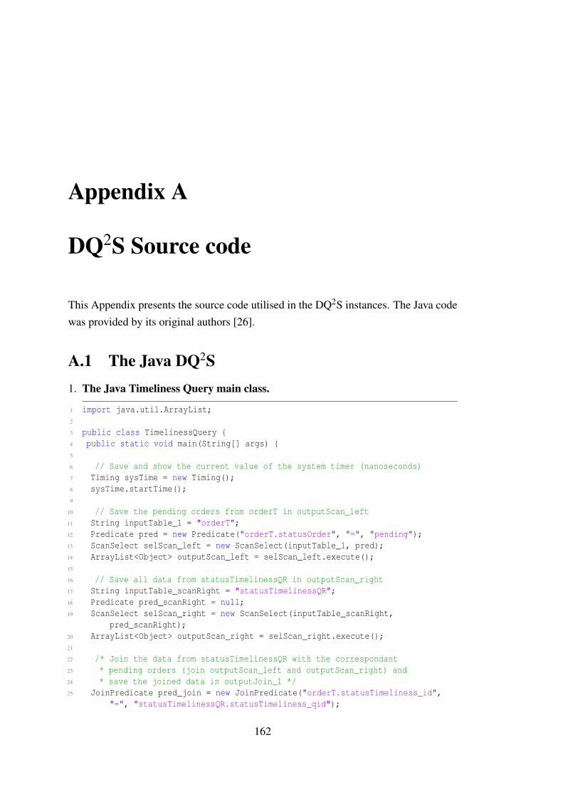
Appendix A
DQ2S Source code
This Appendix presents the source code utilised in the DQ2S instances. The Java codewas provided by its original authors [26].
A.1 The Java DQ2S1. The Java Timeliness Query main class.
1 import java.util.ArrayList;2
3 public class TimelinessQuery 4 public static void main(String[] args) 5
6 // Save and show the current value of the system timer (nanoseconds)7 Timing sysTime = new Timing();8 sysTime.startTime();9
10 // Save the pending orders from orderT in outputScan_left11 String inputTable_1 = "orderT";12 Predicate pred = new Predicate("orderT.statusOrder", "=", "pending");13 ScanSelect selScan_left = new ScanSelect(inputTable_1, pred);14 ArrayList<Object> outputScan_left = selScan_left.execute();15
16 // Save all data from statusTimelinessQR in outputScan_right17 String inputTable_scanRight = "statusTimelinessQR";18 Predicate pred_scanRight = null;19 ScanSelect selScan_right = new ScanSelect(inputTable_scanRight,
pred_scanRight);20 ArrayList<Object> outputScan_right = selScan_right.execute();21
22 /* Join the data from statusTimelinessQR with the correspondant23 * pending orders (join outputScan_left and outputScan_right) and24 * save the joined data in outputJoin_1 */25 JoinPredicate pred_join = new JoinPredicate("orderT.statusTimeliness_id",
"=", "statusTimelinessQR.statusTimeliness_qid");
162
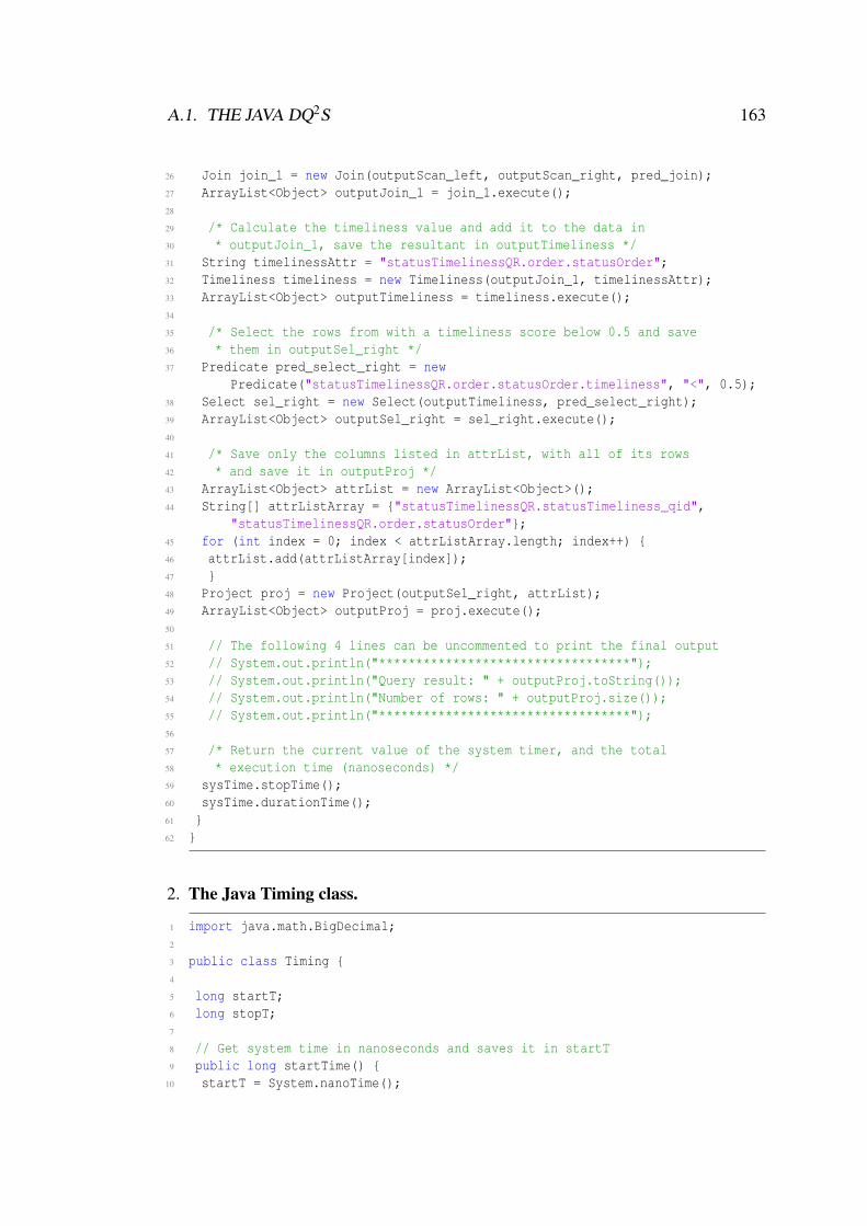
A.1. THE JAVA DQ2S 163
26 Join join_1 = new Join(outputScan_left, outputScan_right, pred_join);27 ArrayList<Object> outputJoin_1 = join_1.execute();28
29 /* Calculate the timeliness value and add it to the data in30 * outputJoin_1, save the resultant in outputTimeliness */31 String timelinessAttr = "statusTimelinessQR.order.statusOrder";32 Timeliness timeliness = new Timeliness(outputJoin_1, timelinessAttr);33 ArrayList<Object> outputTimeliness = timeliness.execute();34
35 /* Select the rows from with a timeliness score below 0.5 and save36 * them in outputSel_right */37 Predicate pred_select_right = new
Predicate("statusTimelinessQR.order.statusOrder.timeliness", "<", 0.5);38 Select sel_right = new Select(outputTimeliness, pred_select_right);39 ArrayList<Object> outputSel_right = sel_right.execute();40
41 /* Save only the columns listed in attrList, with all of its rows42 * and save it in outputProj */43 ArrayList<Object> attrList = new ArrayList<Object>();44 String[] attrListArray = "statusTimelinessQR.statusTimeliness_qid",
"statusTimelinessQR.order.statusOrder";45 for (int index = 0; index < attrListArray.length; index++) 46 attrList.add(attrListArray[index]);47 48 Project proj = new Project(outputSel_right, attrList);49 ArrayList<Object> outputProj = proj.execute();50
51 // The following 4 lines can be uncommented to print the final output52 // System.out.println("**********************************");53 // System.out.println("Query result: " + outputProj.toString());54 // System.out.println("Number of rows: " + outputProj.size());55 // System.out.println("**********************************");56
57 /* Return the current value of the system timer, and the total58 * execution time (nanoseconds) */59 sysTime.stopTime();60 sysTime.durationTime();61 62
2. The Java Timing class.
1 import java.math.BigDecimal;2
3 public class Timing 4
5 long startT;6 long stopT;7
8 // Get system time in nanoseconds and saves it in startT9 public long startTime()
10 startT = System.nanoTime();

164 APPENDIX A. DQ2S SOURCE CODE
11 System.out.println("Process start time in nanoseconds = " +startT);12 return startT;13 14
15 // Get system time in nanoseconds and saves it in stopT16 public long stopTime() 17 stopT = System.nanoTime();18 System.out.println("Process stop time in nanoseconds = " + stopT);19 return stopT;20 21
22 // Calculate elapsed time from the point startT and stopT were obtained23 public void durationTime() 24 long ExecutionDuration = (stopT - startT);25 System.out.println("Process ExecutionDuration in nanoseconds: " +
ExecutionDuration);26 System.out.println("Process ExecutionDuration in seconds: " + (new
BigDecimal ((double) ExecutionDuration/1000000000)));27 28
3. The Java Predicate class.
1 public class Predicate 2 public String operand1;3 public String comparisonOperator;4
5 public Predicate(String inputOperand1, String inputComparisonOperator,Object inputOperand2)
6 public Object operand2;7 operand1 = inputOperand1;8 comparisonOperator = inputComparisonOperator;9 operand2 = inputOperand2;
10 11
12 public boolean apply(Tuple tuple) 13 if (tuple.typeAttributes.contains(operand1)) 14 int positionOfAttribute = tuple.typeAttributes.indexOf(operand1);15 String attributeType = (String)
tuple.typeAttributeTypes.get(positionOfAttribute);16
17 if (attributeType.equals("double"))18 double op_1 = (Double) tuple.tupleValues.get(positionOfAttribute);19 double op_2 = (Double) operand2;20
21 if (comparisonOperator.equals("<")) 22 if (op_1 < op_2) 23 return true;24 25 else if(comparisonOperator.equals("<=")) 26 if (op_1 <= op_2) 27 return true;

A.1. THE JAVA DQ2S 165
28 29 else if(comparisonOperator.equals("=")) 30 if (op_1 == op_2)31 return true;32 else if(comparisonOperator.equals(">")) 33 if (op_1 > op_2)34 return true;35 else if(comparisonOperator.equals(">=")) 36 if (op_1 >= op_2)37 return true;38 else if(comparisonOperator.equals("<>")) 39 if (op_1 != op_2)40 return true;41 42
43 else if (attributeType.equals("int")) 44 int op_1 = (Integer) tuple.tupleValues.get(positionOfAttribute);45 int op_2 = (Integer) operand2;46
47 if (comparisonOperator.equals("<")) 48 if (op_1 < op_2) 49 return true;50 51 else if(comparisonOperator.equals("<=")) 52 if (op_1 <= op_2) 53 return true;54 55 else if(comparisonOperator.equals("=")) 56 if (op_1 == op_2)57 return true;58 else if(comparisonOperator.equals(">")) 59 if (op_1 > op_2)60 return true;61 else if(comparisonOperator.equals(">=")) 62 if (op_1 >= op_2)63 return true;64 else if(comparisonOperator.equals("<>")) 65 if (op_1 != op_2)66 return true;67 68
69 else if (attributeType.equals("String")) 70 String op_1 = (String) tuple.tupleValues.get(positionOfAttribute);71 String op_2 = (String) operand2;72
73 if (comparisonOperator.equals("=")) 74 if (op_1.equals(op_2)) return true;75 else if (comparisonOperator.equals("<>")) 76 if (!(op_1.equals(op_2))) return true;77 78 79 // End if tuple.typeAttributes80 return false; // Return false for predicate

166 APPENDIX A. DQ2S SOURCE CODE
81 // End apply method82
83 public String toString() 84 return ("operand1: " + operand1.toString()85 + "; comparisonOperator: " + comparisonOperator.toString()86 + "; operand2: " + operand2.toString());87 88
89 // End class
4. The Java ScanSelect class.
1 import java.io.BufferedReader;2 import java.io.FileReader;3 import java.util.ArrayList;4 import java.sql.*;5
6 public class ScanSelect 7 public String tableName;8 public Predicate predicate;9 public ArrayList<Object> output;
10
11 public ScanSelect(String inputTableName, Predicate inputPredicate) 12 tableName = inputTableName;13 predicate = inputPredicate;14 output = new ArrayList<Object> ();15 16
17 public ArrayList<Object> execute() 18
19 try 20 // csvFile requires the input data path21 String csvFile = "//local_drive//Ebusiness_DQ2S//"+tableName+".csv";22 String line, splitBy = ",";23
24 BufferedReader rs = new BufferedReader(new FileReader(csvFile));25 rs.readLine(); // Read first line (headers) to "skip" them26
27 boolean discardTuple = false;28
29 while((line = rs.readLine()) != null)30 // Create the tuple object31 Tuple tuple = new Tuple();32 if (tableName.equals("part_supply")) 33 // Resolve tuple type34 String[] data = line.split(splitBy);35 String[] tupleTypeAttributes = "part_supply.supplier_id",
"part_supply.part_id", "part_supply.part_price","part_supply.quantity_available", "part_supply.part_price_qid","part_supply.quantity_qid";
36 String[] tupleTypeAttributeTypes = "int", "int", "double", "int","int", "int";

A.1. THE JAVA DQ2S 167
37 tuple.createType(tupleTypeAttributes, tupleTypeAttributeTypes);38 tuple.tupleValues.add(Integer.parseInt(data[0]));39 tuple.tupleValues.add(Integer.parseInt(data[1]));40 tuple.tupleValues.add(Double.parseDouble(data[2]));41 tuple.tupleValues.add(Integer.parseInt(data[3]));42 tuple.tupleValues.add(Integer.parseInt(data[4]));43 tuple.tupleValues.add(Integer.parseInt(data[5]));44 else if (tableName.equals("part")) 45 // Resolve tuple type46 String[] data = line.split(splitBy);47 String[] tupleTypeAttributes = "part.part_id", "part.part_category",
"part.part_stock";48 String[] tupleTypeAttributeTypes = "int", "String", "int";49 tuple.createType(tupleTypeAttributes, tupleTypeAttributeTypes);50 tuple.tupleValues.add(Integer.parseInt(data[0]));51 tuple.tupleValues.add(data[1]);52 tuple.tupleValues.add(Integer.parseInt(data[2]));53 else if (tableName.equals("statusTimelinessQR")) 54 // Resolve tuple type55 String[] data = line.split(splitBy);56 String[] tupleTypeAttributes =
"statusTimelinessQR.statusTimeliness_qid","statusTimelinessQR.lastUpdateTime","statusTimelinessQR.expiryTime", "statusTimelinessQR.deliveryTime","statusTimelinessQR.age";
57 String[] tupleTypeAttributeTypes = "int", "Timestamp", "Timestamp","Timestamp", "int";
58 tuple.createType(tupleTypeAttributes, tupleTypeAttributeTypes);59 tuple.tupleValues.add(Integer.parseInt(data[0]));60 tuple.tupleValues.add(Timestamp.valueOf(data[1]));61 tuple.tupleValues.add(Timestamp.valueOf(data[2]));62 tuple.tupleValues.add(Timestamp.valueOf(data[3]));63 tuple.tupleValues.add(Integer.parseInt(data[4]));64 else if (tableName.equals("orderT")) 65 // Resolve tuple type66 String[] data = line.split(splitBy);67 String[] tupleTypeAttributes = "orderT.order_no", "orderT.customer_id",
"orderT.product_id", "orderT.quantity", "orderT.submit_date","orderT.ship_date", "orderT.statusTimeliness_id","orderT.statusOrder";
68 String[] tupleTypeAttributeTypes = "int", "int", "int", "int","Timestamp", "Timestamp", "int", "String";
69 tuple.createType(tupleTypeAttributes, tupleTypeAttributeTypes);70 tuple.tupleValues.add(Integer.parseInt(data[0]));71 tuple.tupleValues.add(Integer.parseInt(data[1]));72 tuple.tupleValues.add(Integer.parseInt(data[2]));73 tuple.tupleValues.add(Integer.parseInt(data[3]));74 tuple.tupleValues.add(Timestamp.valueOf(data[4]));75 tuple.tupleValues.add(Timestamp.valueOf(data[5]));76 tuple.tupleValues.add(Integer.parseInt(data[6]));77 tuple.tupleValues.add(data[7]);78 else if (tableName.equals("part_priceTimelinessQR")) 79 // Resolve tuple type

168 APPENDIX A. DQ2S SOURCE CODE
80 String[] data = line.split(splitBy);81 String[] tupleTypeAttributes = "part_priceTimelinessQR.timeliness_qid",
"part_priceTimelinessQR.lastUpdateTime","part_priceTimelinessQR.expiryTime","part_priceTimelinessQR.deliveryTime", "part_priceTimelinessQR.age";
82 String[] tupleTypeAttributeTypes = "int", "Timestamp", "Timestamp","Timestamp", "int";
83 tuple.createType(tupleTypeAttributes, tupleTypeAttributeTypes);84 tuple.tupleValues.add(Integer.parseInt(data[0]));85 tuple.tupleValues.add(Timestamp.valueOf(data[1]));86 tuple.tupleValues.add(Timestamp.valueOf(data[2]));87 tuple.tupleValues.add(Timestamp.valueOf(data[3]));88 tuple.tupleValues.add(Integer.parseInt(data[0]));89 // End if tableName90
91
92 if (predicate != null) 93 discardTuple = predicate.apply(tuple);94 if (discardTuple == true) 95 output.add(tuple);96 97 else output.add(tuple);98
99 // End while rs.next()100
101 rs.close();102 return output;103 // End of try block104
105 catch (Exception e) 106 System.out.println("Driver Registration Exception: " + e.getMessage());107 e.printStackTrace();108 return output;109 110 // End execute method111
112 public String toString() 113 if (predicate != null)114 return ("tableName: " + tableName.toString()115 + "; predicate: " + predicate.toString()116 + "; output: " + output.toString());117 else return ("tableName: " + tableName.toString()118 + "; predicate: null"119 + "; output: " + output.toString());120 121
122 // End class
5. The Java Tuple class.
1 import java.util.*;2

A.1. THE JAVA DQ2S 169
3 public class Tuple 4 public ArrayList<Object> typeAttributes;5 public ArrayList<Object> typeAttributeTypes;6 public ArrayList<Object> tupleValues;7
8 public Tuple() 9 typeAttributes = new ArrayList<Object> ();
10 typeAttributeTypes = new ArrayList<Object> ();11 tupleValues = new ArrayList<Object> ();12 13
14 public boolean createType(String[] inputTypeAttributes, String[]inputTypeAttributeTypes)
15 for (int index = 0; index < inputTypeAttributes.length; index++) 16 typeAttributes.add(inputTypeAttributes[index]);17 typeAttributeTypes.add(inputTypeAttributeTypes[index]);18 19 return true;20 21
22 public String toString_original() 23 return ("typeAttributes: " + typeAttributes.toString()24 + "; typeAttributeTypes: " + typeAttributeTypes.toString()25 + "; tupleValues: " + tupleValues.toString());26 27
28 public String toString() 29 return ("tupleValues: " + tupleValues.toString() + "\n");30 31
6. The Java JoinPredicate class.
1 public class JoinPredicate 2 public String operand1;3 public String comparisonOperator;4 public String operand2;5
6 public JoinPredicate(String inputOperand1, String inputComparisonOperator,String inputOperand2)
7 operand1 = inputOperand1;8 comparisonOperator = inputComparisonOperator;9 operand2 = inputOperand2;
10 11
12 public boolean apply(Tuple tuple) 13 if (tuple.typeAttributes.contains(operand1) &&
(tuple.typeAttributes.contains(operand2))) 14
15 int positionOfAttribute_op1 = tuple.typeAttributes.indexOf(operand1);16 int positionOfAttribute_op2 = tuple.typeAttributes.indexOf(operand2);17

170 APPENDIX A. DQ2S SOURCE CODE
18 String attributeType_op1 = (String)tuple.typeAttributeTypes.get(positionOfAttribute_op1);
19
20 if (attributeType_op1.equals("double")) 21 double op_1 = (Double) tuple.tupleValues.get(positionOfAttribute_op1);22 double op_2 = (Double) tuple.tupleValues.get(positionOfAttribute_op2);23
24 if (comparisonOperator.equals("<"))25 if (op_1 < op_2) 26 return true;27 28 else if(comparisonOperator.equals("<=")) 29 if (op_1 <= op_2) 30 return true;31 32 else if(comparisonOperator.equals("=")) 33 if (op_1 == op_2)34 return true;35 else if(comparisonOperator.equals(">")) 36 if (op_1 > op_2)37 return true;38 else if(comparisonOperator.equals(">=")) 39 if (op_1 >= op_2)40 return true;41 else if(comparisonOperator.equals("<>")) 42 if (op_1 != op_2)43 return true;44 45
46 else if (attributeType_op1.equals("int")) 47 int op_1 = (Integer) tuple.tupleValues.get(positionOfAttribute_op1);48 int op_2 = (Integer) tuple.tupleValues.get(positionOfAttribute_op2);49
50 if (comparisonOperator.equals("<"))51 if (op_1 < op_2) 52 return true;53 54 else if(comparisonOperator.equals("<=")) 55 if (op_1 <= op_2) 56 return true;57 58 else if(comparisonOperator.equals("=")) 59 if (op_1 == op_2)60 return true;61 else if(comparisonOperator.equals(">")) 62 if (op_1 > op_2)63 return true;64 else if(comparisonOperator.equals(">=")) 65 if (op_1 >= op_2)66 return true;67 else if(comparisonOperator.equals("<>")) 68 if (op_1 != op_2)69 return true;

A.1. THE JAVA DQ2S 171
70 71
72 else if (attributeType_op1.equals("String")) 73 String op_1 = (String) tuple.tupleValues.get(positionOfAttribute_op1);74 String op_2 = (String) tuple.tupleValues.get(positionOfAttribute_op2);75 if (comparisonOperator.equals("=")) 76 if (op_1.equals(op_2)) return true;77 else if (comparisonOperator.equals("<>")) 78 if (!(op_1.equals(op_2))) return true;79 80 81 82 return false; // Return false for predicate83 // End apply method84
85 public String toString() 86 return ("operand1: " + operand1.toString()87 + "; comparisonOperator: " + comparisonOperator.toString()88 + "; operand2: " + operand2.toString());89 90 // End class
7. The Java Join class.
1 import java.util.ArrayList;2
3 public class Join 4 public ArrayList<Object> inputLeft;5 public ArrayList<Object> inputRight;6 public JoinPredicate predicate;7 public ArrayList<Object> output;8
9 public Join(ArrayList<Object> inputInputLeft, ArrayList<Object>inputInputRight, JoinPredicate inputPredicate)
10 inputLeft = inputInputLeft;11 inputRight = inputInputRight;12 predicate = inputPredicate;13 output = new ArrayList<Object> ();14 15
16 public ArrayList<Object> execute() 17 Tuple outputTuple = new Tuple();18 boolean discardTuple = false;19
20 // Copy contents of both left and right input into new tuple21 for(int index_inputLeft = 0; index_inputLeft < inputLeft.size();
index_inputLeft++) 22 Tuple currentTuple_left = (Tuple) inputLeft.get(index_inputLeft);23
24 for(int index_inputRight = 0; index_inputRight < inputRight.size();index_inputRight++)
25 outputTuple.tupleValues.addAll(currentTuple_left.tupleValues);

172 APPENDIX A. DQ2S SOURCE CODE
26 outputTuple.typeAttributeTypes.addAll(currentTuple_left.typeAttributeTypes);27 outputTuple.typeAttributes.addAll(currentTuple_left.typeAttributes);28
29 Tuple currentTuple_right = (Tuple) inputRight.get(index_inputRight);30 outputTuple.tupleValues.addAll(currentTuple_right.tupleValues);31 outputTuple.typeAttributeTypes.addAll(currentTuple_right.typeAttributeTypes);32 outputTuple.typeAttributes.addAll(currentTuple_right.typeAttributes);33
34 if (predicate != null) 35 discardTuple = predicate.apply(outputTuple);36 if (discardTuple == true) 37 output.add(outputTuple);38 39 else output.add(outputTuple);40 outputTuple = null;41 outputTuple = new Tuple();42 // End for inputRight43 // End for inputLeft44 return output;45 // End execute method46
47 public String toString() 48 return ("inputLeft: " + inputLeft.toString()49 + "inputRight: " + inputRight.toString()50 + "; predicate: " + predicate.toString()51 + "; output: " + output.toString());52 53 // End class
8. The Java Timeliness class.
1 import java.util.ArrayList;2 import java.sql.*;3
4 public class Timeliness 5 public ArrayList<Object> input;6 public String timelinessAttribute;7 public ArrayList<Object> output;8
9 public Timeliness(ArrayList<Object> inputInput, StringinputTimelinessAttribute)
10 input = inputInput;11 timelinessAttribute = inputTimelinessAttribute;12 output = new ArrayList<Object> ();13 14
15 public ArrayList<Object> execute() 16 for(int index = 0; index < input.size(); index++) 17 Tuple currentTuple = (Tuple) input.get(index);18 Tuple outputTuple = new Tuple();19 Timestamp deliveryTimeValue = new Timestamp(0);20 Timestamp lastUpdateTime = new Timestamp(0);

A.1. THE JAVA DQ2S 173
21 Timestamp expiryTimeValue = new Timestamp(0);22 int age;23 double calculatedTimelinessScore;24
25 // Get the timeliness attributes from the quality relation26 for (int index_tupletype = 0; index_tupletype <
currentTuple.typeAttributes.size(); index_tupletype++) 27 String currentAttribute = (String)
currentTuple.typeAttributes.get(index_tupletype);28 if (currentAttribute.matches("(.*)deliveryTime")) 29 deliveryTimeValue = (Timestamp)
currentTuple.tupleValues.get(index_tupletype);30 else if (currentAttribute.matches("(.*)lastUpdateTime")) 31 lastUpdateTime = (Timestamp)
currentTuple.tupleValues.get(index_tupletype);32 else if (currentAttribute.matches("(.*)age")) 33 age = (Integer) currentTuple.tupleValues.get(index_tupletype);34 else if (currentAttribute.matches("(.*)expiryTime")) 35 expiryTimeValue = (Timestamp)
currentTuple.tupleValues.get(index_tupletype);36 37 // End for index_tupletype38
39 /*Calculate currency and volatility for the current tuple,40 * stored in milliseconds */41 long currencyLong = deliveryTimeValue.getTime() - lastUpdateTime.getTime();42 long volatilityLong = expiryTimeValue.getTime() - lastUpdateTime.getTime();43
44 // Calculate timeliness45 double timelinessPartial = (1 - ((double) currencyLong/volatilityLong));46
47 // Apply max(score, 0)48 double zeroNum = 0.00;49 if (timelinessPartial >= zeroNum) 50 calculatedTimelinessScore = timelinessPartial;51 else calculatedTimelinessScore = zeroNum;52
53 // Create new tuple54 outputTuple.typeAttributes.addAll(currentTuple.typeAttributes);55 outputTuple.typeAttributes.add(timelinessAttribute + ".timeliness");56
57 outputTuple.typeAttributeTypes.addAll(currentTuple.typeAttributeTypes);58 outputTuple.typeAttributeTypes.add("double");59
60 outputTuple.tupleValues.addAll(currentTuple.tupleValues);61 outputTuple.tupleValues.add(calculatedTimelinessScore);62
63 output.add(outputTuple);64 outputTuple = null;65 // End for index66 return output;67 // End execute method68

174 APPENDIX A. DQ2S SOURCE CODE
69 public String toString() 70 return ("input: " + input.toString()71 + "; timelinessAttribute: " + timelinessAttribute.toString()72 + "; output: " + output.toString());73 74 // End class
9. The Java Select class.
1 import java.util.ArrayList;2
3 public class Select 4
5 public ArrayList<Object> input;6 public Predicate predicate;7 public ArrayList<Object> output;8
9 public select(ArrayList<Object> inputInput, Predicate inputPredicate) 10 input = inputInput;11 predicate = inputPredicate;12 output = new ArrayList<Object> ();13 14
15 public ArrayList<Object> execute() 16 boolean retainTuple = false;17 for(int index = 0; index < input.size(); index++) 18 Tuple currentTuple = (Tuple) input.get(index);19 if (predicate != null) 20 retainTuple = predicate.apply(currentTuple);21 if (retainTuple == true) // Proceed to add only tuples with predicate
true value22 output.add(currentTuple);23 24 25 // End for input26 return output;27 // End execute method28
29 public String toString() 30 return ("input: " + input.toString()31 + "; predicate: " + predicate.toString()32 + "; output: " + output.toString());33 34
35
10. The Java Project class.
1 import java.util.ArrayList;2
3 public class Project 4 public ArrayList<Object> input;

A.2. THE PYTHON DQ2S 175
5 public ArrayList<Object> attributeList;6 public ArrayList<Object> output;7
8 public Project(ArrayList<Object> inputInput, ArrayList<Object>inputAttributeList)
9 input = inputInput;10 attributeList = inputAttributeList;11 output = new ArrayList<Object> ();12 13
14 public ArrayList<Object> execute() 15 for(int index = 0; index < input.size(); index++) 16 Tuple currentTuple = (Tuple) input.get(index);17 Tuple outputTuple = new Tuple();18 for (int index_tupletype = 0; index_tupletype <
currentTuple.typeAttributes.size(); index_tupletype++) 19 for (int index_attrList = 0; index_attrList < attributeList.size();
index_attrList++) 20 if
(currentTuple.typeAttributes.get(index_tupletype).equals(attributeList.get(index_attrList)))
21 outputTuple.typeAttributes.add(currentTuple.typeAttributes.get(index_tupletype));22 outputTuple.typeAttributeTypes.add(currentTuple.typeAttributeTypes.get(index_tupletype));23 outputTuple.tupleValues.add(currentTuple.tupleValues.get(index_tupletype));24 25 // End for attributesList26 // End for index_tupletype27 output.add(outputTuple);28 outputTuple = null;29 outputTuple = new Tuple();30 // End for input.size31 return output;32 // End execute method33
34 public String toString() 35 return ("input: " + input.toString()36 + "; attributeList: " + attributeList.toString()37 + "; output: " + output.toString());38 39
A.2 The Python DQ2S
1. The Python Timeliness Query main class.
1 from Timing import Timing2 from Predicate import Predicate3 from ScanSelect import ScanSelect4 from JoinPredicate import JoinPredicate5 from Join import Join

176 APPENDIX A. DQ2S SOURCE CODE
6 from Timeliness import Timeliness7 from Select import Select8 from Project import Project9
10 class Query2():11
12 timing = Timing()13 startTime = timing.startTime()14
15 # Create a ScanSelect_left --> only pending orders16 inputTable_1 = ’orderT’17 predScan_left = Predicate(’orderT.statusOrder’, ’=’, ’pending’)18 selScan_left = ScanSelect(inputTable_1, predScan_left)19 outputScan_left = selScan_left.execute()20
21 # Create a ScanSelect_right --> all from statusTimelinessQR22 inputTable_2 = "statusTimelinessQR"23 predScan_right = None24 selScan_right = ScanSelect(inputTable_2, predScan_right)25 outputScan_right = selScan_right.execute()26
27 # Create a Join --> outputScan_left and ouputScan_left28 predJoin = JoinPredicate("orderT.statusTimeliness_id", "=",
"statusTimelinessQR.statusTimeliness_qid")29 join_1 = Join(outputScan_left, outputScan_right, predJoin)30 outputJoin_1 = join_1.execute()31
32 # Calculate timeliness score33 timelinessAttr = "timeliness"34 timeliness = Timeliness(outputJoin_1, timelinessAttr);35 outputTimeliness = timeliness.execute()36
37 # Create a Select --> score < 0.538 predSelect_right = Predicate("timeliness.score", "<", 0.5)39 sel_right = Select(outputTimeliness, predSelect_right)40 outputSel_right = sel_right.execute();41
42 # Creating a Project --> only columns in attrList43 attrList = []44 attrListArray =
["statusTimelinessQR.statusTimeliness_qid","timeliness.score"]45 for index, val in enumerate(attrListArray):46 attrList.append(attrListArray[index])47
48 proj = Project(outputSel_right, attrList)49 outputFinal = proj.execute()50
51 # Uncomment to print final output52 ’’’53 for r in outputFinal:54 print(r.valueAttributes)55 print(len(outputFinal))56 ’’’

A.2. THE PYTHON DQ2S 177
57
58 stopTime = timing.stopTime()59 timing.durationTime(stopTime, startTime)
2. The Python Timing class.
1 import time2
3 class Timing():4
5 def startTime(self):6 queryStartTime = int(round(time.time()* 1e9))7 print("Query start time in nanoseconds = " + str(queryStartTime))8 return queryStartTime9
10 def stopTime(self):11 queryStopTime = int(round(time.time()* 1e9))12 print("Query stop time in nanoseconds = " + str(queryStopTime))13 return queryStopTime14
15 def durationTime(self,queryStopTime,queryStartTime):16 queryExecutionDuration = (queryStopTime - queryStartTime)17 print("queryExecutionDuration in nanoseconds: " +
str(queryExecutionDuration))18 print("queryExecutionDuration in seconds: " +
str((queryExecutionDuration/1000000000)))
3. The Python Predicate class.
1 class Predicate():2
3 def __init__(self, inputOperand1, inputComparisonOperator, inputOperand2):4 self.operand1 = inputOperand15 self.comparisonOperator = inputComparisonOperator6 self.operand2 = inputOperand27
8 def apply(self,tuple1):9 if (self.operand1 in tuple1.nameAttributes):
10 positionOfAttribute = tuple1.nameAttributes.index(self.operand1)11 self.attributeType =
str(tuple1.typeAttributes[positionOfAttribute])12
13 if (self.attributeType == "double"):14 op_1 = float(tuple1.valueAttributes[positionOfAttribute])15 op_2 = float(self.operand2)16
17 if (self.comparisonOperator == "<"):18 if (op_1 < op_2):19 return True20 elif(self.comparisonOperator == "<="):21 if (op_1 <= op_2):22 return True
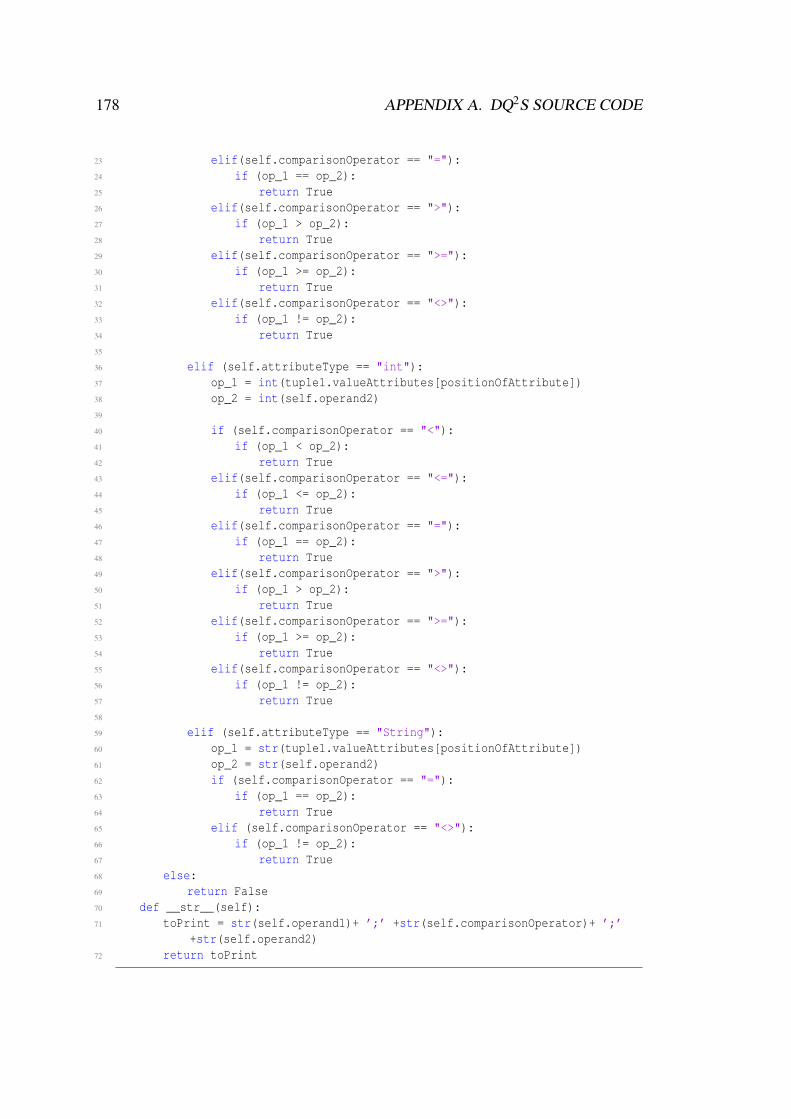
178 APPENDIX A. DQ2S SOURCE CODE
23 elif(self.comparisonOperator == "="):24 if (op_1 == op_2):25 return True26 elif(self.comparisonOperator == ">"):27 if (op_1 > op_2):28 return True29 elif(self.comparisonOperator == ">="):30 if (op_1 >= op_2):31 return True32 elif(self.comparisonOperator == "<>"):33 if (op_1 != op_2):34 return True35
36 elif (self.attributeType == "int"):37 op_1 = int(tuple1.valueAttributes[positionOfAttribute])38 op_2 = int(self.operand2)39
40 if (self.comparisonOperator == "<"):41 if (op_1 < op_2):42 return True43 elif(self.comparisonOperator == "<="):44 if (op_1 <= op_2):45 return True46 elif(self.comparisonOperator == "="):47 if (op_1 == op_2):48 return True49 elif(self.comparisonOperator == ">"):50 if (op_1 > op_2):51 return True52 elif(self.comparisonOperator == ">="):53 if (op_1 >= op_2):54 return True55 elif(self.comparisonOperator == "<>"):56 if (op_1 != op_2):57 return True58
59 elif (self.attributeType == "String"):60 op_1 = str(tuple1.valueAttributes[positionOfAttribute])61 op_2 = str(self.operand2)62 if (self.comparisonOperator == "="):63 if (op_1 == op_2):64 return True65 elif (self.comparisonOperator == "<>"):66 if (op_1 != op_2):67 return True68 else:69 return False70 def __str__(self):71 toPrint = str(self.operand1)+ ’;’ +str(self.comparisonOperator)+ ’;’
+str(self.operand2)72 return toPrint

A.2. THE PYTHON DQ2S 179
4. The Python ScanSelect class.
1 import csv2 from Tuple import Tuple3
4 class ScanSelect():5
6 def __init__(self, inputTableName, inputPredicate):7 self.tableName = inputTableName8 self.predicate = inputPredicate9 self.output = []
10
11 def execute(self):12 # csvFile requires the input data local path13 csvFile = open(’//local_drive//eBusiness//’+self.tableName+’.csv’)14 csvReader = csv.reader(csvFile)15 discardTuple = False16
17 for row in csvReader:18 if csvReader.line_num == 1:19 continue # Skip first row20 tuple1 = Tuple()21 if (self.tableName == ’orderT’):22 data = [row]23 nameAttributes = ["orderT.order_no", "orderT.customer_id",
"orderT.product_id", "orderT.quantity","orderT.submit_date", "orderT.ship_date","orderT.statusTimeliness_id", "orderT.statusOrder"]
24 typeAttributes = ["int", "int", "int", "int", "Timestamp","Timestamp", "int", "String"]
25 tuple1.createType(nameAttributes,typeAttributes)26 tuple1.valueAttributes.append(int(data[0][0]))27 tuple1.valueAttributes.append(int(data[0][1]))28 tuple1.valueAttributes.append(int(data[0][2]))29 tuple1.valueAttributes.append(int(data[0][3]))30 tuple1.valueAttributes.append(str(data[0][4]))31 tuple1.valueAttributes.append(str(data[0][5]))32 tuple1.valueAttributes.append(int(data[0][6]))33 tuple1.valueAttributes.append(str(data[0][7]))34
35 elif (self.tableName == ’statusTimelinessQR’):36 data = [row]37 nameAttributes = ["statusTimelinessQR.statusTimeliness_qid",
"statusTimelinessQR.lastUpdateTime","statusTimelinessQR.expiryTime","statusTimelinessQR.deliveryTime","statusTimelinessQR.age"]
38 typeAttributes = ["int", "Timestamp", "Timestamp","Timestamp", "int"]
39 tuple1.createType(nameAttributes,typeAttributes)40 tuple1.valueAttributes.append(int(data[0][0]))41 tuple1.valueAttributes.append(str(data[0][1]))42 tuple1.valueAttributes.append(str(data[0][2]))

180 APPENDIX A. DQ2S SOURCE CODE
43 tuple1.valueAttributes.append(str(data[0][3]))44 tuple1.valueAttributes.append(int(data[0][4]))45
46 if (self.predicate != None):47 self.discardTuple = self.predicate.apply(tuple1);48 if (self.discardTuple == True):49 self.output.append(tuple1)50
51 else:52 self.output.append(tuple1)53
54 return self.output55
56 def __str__(self):57 if self.predicate != None:58 toPrint = ’TableName: ’ +str(self.tableName)+ ’\nPredicate: ’
+str(self.predicate)+ ’\nOutput: ’ +str(self.output)59 return toPrint60 else:61 toPrint = ’TableName: ’ +str(self.tableName)+ ’\nPredicate: NULL
\nOutput: ’ +str(self.output)62 return toPrint
5. The Python Tuple class.
1 class Tuple():2
3 def __init__(self):4 self.nameAttributes = []5 self.typeAttributes = []6 self.valueAttributes = []7
8 def createType(self, inputNameAttributes, inputTypeAttributes):9 for index, val in enumerate(inputNameAttributes):
10 self.nameAttributes.append(inputNameAttributes[index])11 self.typeAttributes.append(inputTypeAttributes[index])12 return True13
14 def __str__(self):15 toPrint = str(self.nameAttributes)+ ’;’ +str(self.typeAttributes)+
’;’ +str(self.valueAttributes)16 return toPrint
6. The Python JoinPredicate class.
1 class JoinPredicate():2
3 def __init__(self, inputOperand1, inputComparisonOperator, inputOperand2):4 self.operand1 = inputOperand15 self.comparisonOperator = inputComparisonOperator6 self.operand2 = inputOperand27

A.2. THE PYTHON DQ2S 181
8 def apply(self,tuple1):9 if (self.operand1 in tuple1.nameAttributes and self.operand2 in
tuple1.nameAttributes):10 positionOfAttribute_op1 =
tuple1.nameAttributes.index(self.operand1)11 positionOfAttribute_op2 =
tuple1.nameAttributes.index(self.operand2)12
13 self.attributeType_op1 = str(tuple1.typeAttributes[positionOfAttribute_op1])
14
15 if (self.attributeType_op1 == "double"):16 op_1 = Double(tuple1.valueAttributes[positionOfAttribute_op1])17 op_2 = Double(tuple1.valueAttributes[positionOfAttribute_op2])18
19 if (self.comparisonOperator == "<"):20 if (op_1 < op_2):21 return True22 elif(self.comparisonOperator == "<="):23 if (op_1 <= op_2):24 return True25 elif(self.comparisonOperator == "="):26 if (op_1 == op_2):27 return True28 elif(self.comparisonOperator == ">"):29 if (op_1 > op_2):30 return True31 elif(self.comparisonOperator == ">="):32 if (op_1 >= op_2):33 return True34 elif(self.comparisonOperator == "<>"):35 if (op_1 != op_2):36 return True37
38 elif (self.attributeType_op1 == "int"):39 op_1 = int(tuple1.valueAttributes[positionOfAttribute_op1])40 op_2 = int(tuple1.valueAttributes[positionOfAttribute_op2])41
42 if (self.comparisonOperator == "<"):43 if (op_1 < op_2):44 return True45 elif(self.comparisonOperator == "<="):46 if (op_1 <= op_2):47 return True48 elif(self.comparisonOperator == "="):49 if (op_1 == op_2):50 return True51 elif(self.comparisonOperator == ">"):52 if (op_1 > op_2):53 return True54 elif(self.comparisonOperator == ">="):55 if (op_1 >= op_2):56 return True

182 APPENDIX A. DQ2S SOURCE CODE
57 elif(self.comparisonOperator == "<>"):58 if (op_1 != op_2):59 return True60
61 elif (self.attributeType_op1 == "String"):62
63 op_1 = str(tuple1.valueAttributes[positionOfAttribute_op1])64 op_2 = str(tuple1.valueAttributes[positionOfAttribute_op2])65 if (self.comparisonOperator == "="):66 if (op_1 == op_2):67 return True68 elif (self.comparisonOperator == "<>"):69 if (op_1 != op_2):70 return True71 else:72 return False73
74 def __str__(self):75 toPrint = str(self.operand1)+ ’;’ +str(self.comparisonOperator)+ ’;’
+str(self.operand2)76 return toPrint
7. The Python Join class.
1 from Tuple import Tuple2
3 class Join():4
5 def __init__(self, inputInputLeft, inputInputRight, inputPredicate):6 self.inputLeft = inputInputLeft7 self.inputRight = inputInputRight8 self.predicateJoin = inputPredicate9 self.output = []
10
11 def execute(self):12
13 outputTuple = Tuple()14 discardTuple = False15
16 for indexInput_left, val in enumerate(self.inputLeft):17 currentTuple_left = self.inputLeft[indexInput_left]18
19 for indexInput_right, val in enumerate(self.inputRight):20 outputTuple.valueAttributes.extend(currentTuple_left.valueAttributes)21 outputTuple.typeAttributes.extend(currentTuple_left.typeAttributes)22 outputTuple.nameAttributes.extend(currentTuple_left.nameAttributes)23
24 currentTuple_right = self.inputRight[indexInput_right]25 outputTuple.valueAttributes.extend(currentTuple_right.valueAttributes);26 outputTuple.typeAttributes.extend(currentTuple_right.typeAttributes);27 outputTuple.nameAttributes.extend(currentTuple_right.nameAttributes);28

A.2. THE PYTHON DQ2S 183
29 if self.predicateJoin != None:30
31 discardTuple = self.predicateJoin.apply(outputTuple);32 if discardTuple == True:33 self.output.append(outputTuple)34 else:35 self.output.append(outputTuple)36 outputTuple = None;37 outputTuple = Tuple()38 return self.output;39
40 def __str__(self):41 toPrint = str(self.inputLeft)+ ’;’ +str(self.inputRight)+ ’;’
+str(self.predicate)+ ’;’ +str(self.output)42 return toPrint
8. The Python Timeliness class.
1 from Tuple import Tuple2 import re3 import time4 from datetime import datetime5
6 class Timeliness():7
8 def __init__(self, inputInput, inputTimelinessAttr):9 self.input = inputInput
10 self.timelinessAttr = inputTimelinessAttr11 self.output = []12
13 def execute(self):14 # Convert timestamp to epoch time in milliseconds15 def to_unix_time(timestamp):16 epoch = datetime.utcfromtimestamp(0)17 my_time = datetime.strptime(timestamp, ’%Y-%m-%d %H:%M:%S’)18 delta = my_time - epoch19 return delta.total_seconds() * 1000.020
21 for index,val in enumerate(self.input):22 currentTuple = self.input[index]23 outputTuple = Tuple()24
25 for index_tupletype,val in enumerate(currentTuple.nameAttributes):26 currentAttribute =
str(currentTuple.nameAttributes[index_tupletype])27
28 if re.match("(.*)deliveryTime", currentAttribute) != None:29 deliveryTime_str =
currentTuple.valueAttributes[index_tupletype]30 elif re.match("(.*)lastUpdateTime", currentAttribute) != None:31 lastUpdateTime_str =
currentTuple.valueAttributes[index_tupletype]

184 APPENDIX A. DQ2S SOURCE CODE
32 elif re.match("(.*)age", currentAttribute) != None:33 age = int(currentTuple.valueAttributes[index_tupletype])34 elif re.match("(.*)expiryTime",currentAttribute) != None:35 expiryTime_str =
currentTuple.valueAttributes[index_tupletype]36
37 # Calculate Timeliness Score38 currencyLong = (to_unix_time(deliveryTime_str)-
to_unix_time(lastUpdateTime_str))39 volatilityLong = (to_unix_time(expiryTime_str) -
to_unix_time(lastUpdateTime_str))40 timelinessPartial = (1- (currencyLong/volatilityLong))41
42 # Apply max(score,0)43 zeroNum = 0.0044 if timelinessPartial >= 0.00:45 timelinessScore = timelinessPartial46 else:47 timelinessScore = zeroNum48
49 # Create new tuple50 outputTuple.nameAttributes.extend(currentTuple.nameAttributes)51 outputTuple.nameAttributes.append(self.timelinessAttr + ".score")52
53 outputTuple.typeAttributes.extend(currentTuple.typeAttributes)54 outputTuple.typeAttributes.append("double")55 outputTuple.valueAttributes.extend(currentTuple.valueAttributes)56 outputTuple.valueAttributes.append(timelinessScore)57 self.output.append(outputTuple)58 outputTuple = None59
60 return self.output61
62 def __str__(self):63 toPrint = str(self.input)+ ’;’ +str(self.timelinessAttr)+ ’;’
+str(self.output)64 return toPrint
9. The Python Select class.
1 from Tuple import Tuple2
3 class Select():4
5 def __init__(self, inputInput, inputPredicate):6 self.input = inputInput7 self.predicate = inputPredicate8 self.output = []9
10 def execute(self):11 retainTuple = False12 for index, val in enumerate(self.input):

A.2. THE PYTHON DQ2S 185
13 currentTuple = Tuple()14 currentTuple = self.input[index]15 if self.predicate != None:16 retainTuple = self.predicate.apply(currentTuple)17 if retainTuple == True:18 self.output.append(currentTuple)19 return self.output20
21 def __str__(self):22 toPrint = str(self.input)+ ’;’ +str(self.predicate)+ ’;’
+str(self.output)23 return toPrint
10. The Python Project class.
1 from Tuple import Tuple2
3 class Project():4
5 def __init__(self, inputInput, inputAttrList):6 self.input = inputInput7 self.attrList = inputAttrList8 self.output = []9
10 def execute(self):11 for index, val in enumerate(self.input):12 currentTuple = self.input[index]13 outputTuple = Tuple()14 for index_tupletype,val in enumerate(currentTuple.nameAttributes):15 for index_attrList, val in enumerate(self.attrList):16 if currentTuple.nameAttributes[index_tupletype] ==
self.attrList[index_attrList]:17 outputTuple.nameAttributes.append
(currentTuple.nameAttributes[index_tupletype])18 outputTuple.typeAttributes.append
(currentTuple.typeAttributes[index_tupletype])19 outputTuple.valueAttributes.append
(currentTuple.valueAttributes[index_tupletype])20 self.output.append(outputTuple)21 self.outputTuple = None22 outputTuple = Tuple();23 return self.output24
25 def __str__(self):26 toPrint = str(self.input)+ ’;’ +str(self.attrList)+ ’;’
+str(self.output)27 return toPrint

186 APPENDIX A. DQ2S SOURCE CODE
A.3 The Optimised Python DQ2S
1. The Optimised Python Timeliness Query main class.
1 from Timing import Timing2 from Predicate import Predicate3 from ScanSelect import ScanSelect4 from Join import Join5 from Timeliness import Timeliness6 from Select import Select7 from Project import Project8 import numpy as np9 import pandas as pd
10
11 class Query2():12
13 timing = Timing()14 startTime = timing.startTime()15
16 # Creating a ScanSelect_left --> Only pending orders17 inputTable_1 = ’orderT’18 predScan_left = Predicate(’statusOrder’, ’=’, ’pending’)19 selScan_left = ScanSelect(inputTable_1, predScan_left)20 outputScan_left = selScan_left.execute()21
22 # Creating a ScanSelect_right --> All from statusTimelinessQR23 inputTable_2 = "statusTimelinessQR"24 predScan_right = None25 selScan_right = ScanSelect(inputTable_2, predScan_right)26 outputScan_right = selScan_right.execute()27
28 #Creating a Join --> Join outputScan_left and ouputScan_left29 predJoin = ("statusTimeliness_id", "=", "statusTimeliness_qid")30 join_1 = Join(outputScan_left, outputScan_right, predJoin)31 outputJoin_1 = join_1.execute()32
33 #Creating Timeliness --> Calculate timeliness score34 timelinessAttr = "timeliness"35 timeliness = Timeliness(outputJoin_1, timelinessAttr);36 outputTimeliness = timeliness.execute()37
38 #Creating a Select --> Select those with Timeliness < 0.539 predSelect_right = Predicate("timeliness_score", "<", 0.5)40 sel_right = Select(outputTimeliness, predSelect_right)41 outputSel_right = sel_right.execute();42
43 #Creating a Project --> Short the DF to have only two columns44 attrList = ["statusTimeliness_qid","timeliness_score"]45 proj = Project(outputSel_right, attrList)46 outputFinal = proj.execute()47
48 # Uncomment to print final output

A.3. THE OPTIMISED PYTHON DQ2S 187
49 ’’’50 n = len(outputFinal.index)51 print(outputFinal.head(n).to_string())52 print("Project Output= ")53 print(n)54 ’’’55
56 stopTime = timing.stopTime()57 timing.durationTime(stopTime, startTime)
2. The Optimised Python Timing class.
1 import time2
3 class Timing():4
5 def startTime(self):6 queryStartTime = int(round(time.time()* 1e9))7 print("Query start time in nanoseconds = " + str(queryStartTime))8 return queryStartTime9
10 def stopTime(self):11 queryStopTime = int(round(time.time()* 1e9))12 print("Query stop time in nanoseconds = " + str(queryStopTime))13 return queryStopTime14
15 def durationTime(self,queryStopTime,queryStartTime):16 queryExecutionDuration = (queryStopTime - queryStartTime)17 print("queryExecutionDuration in nanoseconds: " +
str(queryExecutionDuration))18 print("queryExecutionDuration in seconds: " +
str((queryExecutionDuration/1000000000)))
3. The Optimised Python Predicate class.
1 class Predicate():2
3 def __init__(self, inputOperand1, inputComparisonOperator, inputOperand2):4 self.operand1 = inputOperand15 self.comparisonOperator = inputComparisonOperator6 self.operand2 = inputOperand27
8 def apply(self,dfInput):9 operand1_true = 0
10 nameAttributes = dfInput.columns11 typeAttributes = dfInput.dtypes12 if (self.operand1 in nameAttributes):13 positionOfAttribute = nameAttributes.get_loc(self.operand1)14 attributeType = str(typeAttributes[positionOfAttribute])15 operand1_true = 116
17 if (operand1_true != 0):

188 APPENDIX A. DQ2S SOURCE CODE
18
19 if (attributeType != "object"):20 self.operand1 = str(self.operand1)21 op_2 = str(self.operand2)22 if (self.comparisonOperator == "<"):23 filterClause = ""+self.operand1+"<"+op_2+""24 print(filterClause)25 dfOutput = dfInput.query(filterClause)26 elif(self.comparisonOperator == "<="):27 filterClause = ""+self.operand1+"<="+op_2+""28 dfOutput = dfInput.query(filterClause)29 elif(self.comparisonOperator == "="):30 filterClause = ""+self.operand1+"="+op_2+""31 dfOutput = dfInput.query(filterClause)32 elif(self.comparisonOperator == ">"):33 filterClause = ""+self.operand1+">"+op_2+""34 dfOutput = dfInput.query(filterClause)35 elif(self.comparisonOperator == ">="):36 filterClause = ""+self.operand1+">="+op_2+""37 dfOutput = dfInput.query(filterClause)38 elif(self.comparisonOperator == "<>"):39 filterClause = ""+self.operand1+"!="+op_2+""40 dfOutput = dfInput.query(filterClause)41
42 elif (attributeType == "object"):43 op_2 = str(self.operand2)44 if(self.comparisonOperator == "="):45 filterClause = ""+self.operand1+"==’"+op_2+"’"46 dfOutput = dfInput.query(filterClause)47 elif(self.comparisonOperator == "<>"):48 filterClause = ""+self.operand1+"!=’"+op_2+"’"49 dfOutput = dfInput.query(filterClause)50 return dfOutput51 else:52 return dfInput
4. The Optimised Python ScanSelect class.
1 import csv2 import numpy as np3 import pandas as pd4 from datetime import datetime5
6 class ScanSelect():7
8 def __init__(self, inputTableName, inputPredicate):9 self.tableName = inputTableName
10 self.predicate = inputPredicate11 self.output = []12
13 def execute(self):14 if (self.tableName == ’orderT’):

A.3. THE OPTIMISED PYTHON DQ2S 189
15 nameAttributes = ["order_no", "customer_id", "product_id", "quantity","submit_date", "ship_date", "statusTimeliness_id", "statusOrder"]
16 elif (self.tableName == ’statusTimelinessQR’):17 nameAttributes = ["statusTimeliness_qid", "lastUpdateTime", "expiryTime",
"deliveryTime", "age"]18 # dfInput requires the input data local path19 dfInput = pd.read_csv(’//local_drive//eBusiness//’+self.tableName+’.csv’,
names=nameAttributes, header=0, encoding=’latin-1’)20
21 if (self.predicate != None):22 discardTuple = self.predicate.apply(dfInput)23 dfOutput = discardTuple24
25 else:26 dfOutput = dfInput27 return dfOutput
5. The Optimised Python Join class.
1 class Join():2
3 def __init__(self, inputInputLeft, inputInputRight, inputPredicate):4 self.inputLeft = inputInputLeft5 self.inputRight = inputInputRight6 self.predicateJoin = inputPredicate7 self.output = []8
9 def execute(self):10 if self.predicateJoin != None:11 columnName1 = self.inputLeft.columns12 columnName2 = self.inputRight.columns13 operand1 = self.predicateJoin[0]14 comparisonOperator = self.predicateJoin[1]15 operand2 = self.predicateJoin[2]16 operands = [operand1,operand2]17 if (operand1 in columnName1 and operand2 in columnName2 and
comparisonOperator == "="):18 dfOutput = self.inputLeft.merge(self.inputRight, left_on=operand1,
right_on= operand2, how="left")19 else:20 dfOuput = self.inputLeft.join(self.inputRight)21 else:22 dfOuput = self.inputLeft.join(self.inputRight)23 return dfOutput
6. The Optimised Python Timeliness class.
1 import re2 import time3 from datetime import datetime4 import numpy as np5 import pandas as pd
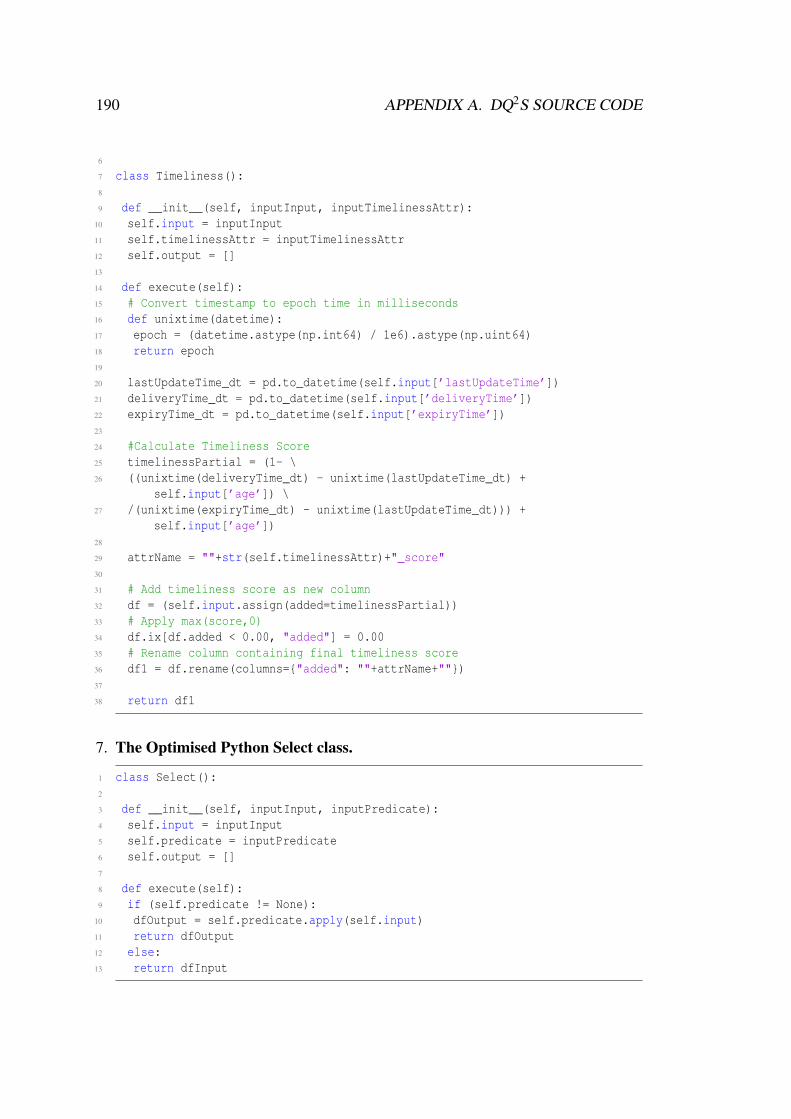
190 APPENDIX A. DQ2S SOURCE CODE
6
7 class Timeliness():8
9 def __init__(self, inputInput, inputTimelinessAttr):10 self.input = inputInput11 self.timelinessAttr = inputTimelinessAttr12 self.output = []13
14 def execute(self):15 # Convert timestamp to epoch time in milliseconds16 def unixtime(datetime):17 epoch = (datetime.astype(np.int64) / 1e6).astype(np.uint64)18 return epoch19
20 lastUpdateTime_dt = pd.to_datetime(self.input[’lastUpdateTime’])21 deliveryTime_dt = pd.to_datetime(self.input[’deliveryTime’])22 expiryTime_dt = pd.to_datetime(self.input[’expiryTime’])23
24 #Calculate Timeliness Score25 timelinessPartial = (1- \26 ((unixtime(deliveryTime_dt) - unixtime(lastUpdateTime_dt) +
self.input[’age’]) \27 /(unixtime(expiryTime_dt) - unixtime(lastUpdateTime_dt))) +
self.input[’age’])28
29 attrName = ""+str(self.timelinessAttr)+"_score"30
31 # Add timeliness score as new column32 df = (self.input.assign(added=timelinessPartial))33 # Apply max(score,0)34 df.ix[df.added < 0.00, "added"] = 0.0035 # Rename column containing final timeliness score36 df1 = df.rename(columns="added": ""+attrName+"")37
38 return df1
7. The Optimised Python Select class.
1 class Select():2
3 def __init__(self, inputInput, inputPredicate):4 self.input = inputInput5 self.predicate = inputPredicate6 self.output = []7
8 def execute(self):9 if (self.predicate != None):
10 dfOutput = self.predicate.apply(self.input)11 return dfOutput12 else:13 return dfInput

A.4. THE PYSPARK DQ2S 191
8. The Optimised Python Project class.
1 class Project():2
3 def __init__(self, inputInput, inputAttrList):4 self.input = inputInput5 self.attrList = inputAttrList6 self.output = []7
8 def execute(self):9 dfRes = self.input[self.attrList]
10 return dfRes
A.4 The PySpark DQ2S
1. The PySpark Timeliness Query main class.
1 from __future__ import print_function2 from pyspark.sql.column import Column, _to_java_column, _to_seq3 from pyspark.sql.dataframe import DataFrame4 from pyspark import SparkConf, SparkContext5 from pyspark.sql import SQLContext, Row6 from pyspark.sql.functions import *7 from pyspark.sql import functions as F8 from pyspark.sql.types import *9 from datetime import datetime
10 import sys11 import math12 from Timing import Timing13 from Predicate import Predicate14 from ScanSelect import ScanSelect15 from Join import Join16 from Timeliness import Timeliness17 from Select import Select18 from Project import Project19
20 # USAGE: bin/spark-submit --packages com.databricks:spark-csv_2.11:1.3.0TimelinessQuery.py appName outputFolderName
21
22 # URL must be replaced by the master address23 # Used for utilisation in local machine or when having full control24 # Commented when used in cluster without admin control25 sc = SparkContext("spark://URL:7077", sys.argv[1],"$SPARK_HOME")26
27 # Uncommented when used in cluster without admin control28 # sc = SparkContext()29
30 sqlContext = SQLContext(sc)31
32 timing = Timing()

192 APPENDIX A. DQ2S SOURCE CODE
33 startTime = timing.startTime()34
35 # Create a ScanSelect_left --> only pending orders36 inputTable_1 = ’orderT’37 predScan_left = Predicate(’statusOrder’, ’=’, ’pending’)38 selScan_left = ScanSelect(inputTable_1, predScan_left, sqlContext)39 dfOutputScan_left = selScan_left.execute()40
41 # Create a ScanSelect_right --> All from statusTimelinessQR42 inputTable_2 = "statusTimelinessQR"43 predScan_right = None44 selScan_right = ScanSelect(inputTable_2, predScan_right, sqlContext)45 dfOutputScan_right = selScan_right.execute()46
47 # Create a Join --> Joining outputScan_left and ouputScan_right48 predJoin = ("statusTimeliness_id", "=", "statusTimeliness_qid")49 dfJoin_1 = Join(dfOutputScan_left, dfOutputScan_right, predJoin)50 dfOutputJoin_1 = dfJoin_1.execute()51
52 # Create Timeliness (add a new column with the calculated timeliness53 timelinessAttr = "timeliness"54 timeliness = Timeliness(dfOutputJoin_1, timelinessAttr)55 dfOutputTimeliness = timeliness.execute()56
57 # Create a Select (extracting only that are true with the condition)58 predSelect_right = Predicate("timeliness_score", "<", 0.5)59 sel_right = Select(dfOutputTimeliness, predSelect_right)60 dfOutputSel_right = sel_right.execute()61
62 # Create a Project (shorting the DF to have only two columns)63 attrList = ["statusTimeliness_qid","timeliness_score"]64 proj = Project(dfOutputSel_right, attrList)65 dfOutputFinal = proj.execute()66
67 # Uncomment next four lines to print full output68 # nrows = dfOutputFinal.count()69 # dfOutputTimeliness.show(nrows,truncate=False)70 # print("Project Output= ")71 # print(nrows)72
73 ’’’74 An action is mandatory to trigger full processing75 due to Spark’s lazy evaluation.76 Show is the less costly action.77 ’’’78 dfOutputFinal.show(1)79
80 stopTime = timing.stopTime()81 timing.durationTime(stopTime, startTime)
2. The PySpark Timing class.
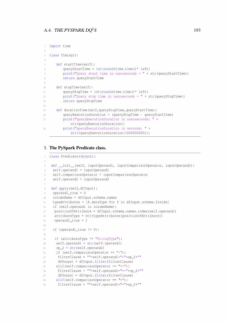
A.4. THE PYSPARK DQ2S 193
1 import time2
3 class Timing():4
5 def startTime(self):6 queryStartTime = int(round(time.time()* 1e9))7 print("Query start time in nanoseconds = " + str(queryStartTime))8 return queryStartTime9
10 def stopTime(self):11 queryStopTime = int(round(time.time()* 1e9))12 print("Query stop time in nanoseconds = " + str(queryStopTime))13 return queryStopTime14
15 def durationTime(self,queryStopTime,queryStartTime):16 queryExecutionDuration = (queryStopTime - queryStartTime)17 print("queryExecutionDuration in nanoseconds: " +
str(queryExecutionDuration))18 print("queryExecutionDuration in seconds: " +
str((queryExecutionDuration/1000000000)))
3. The PySpark Predicate class.
1 class Predicate(object):2
3 def __init__(self, inputOperand1, inputComparisonOperator, inputOperand2):4 self.operand1 = inputOperand15 self.comparisonOperator = inputComparisonOperator6 self.operand2 = inputOperand27
8 def apply(self,dfInput):9 operand1_true = 0
10 columnName = dfInput.schema.names11 typeAttributes = [f.dataType for f in dfInput.schema.fields]12 if (self.operand1 in columnName):13 positionOfAttribute = dfInput.schema.names.index(self.operand1)14 attributeType = str(typeAttributes[positionOfAttribute])15 operand1_true = 116
17 if (operand1_true != 0):18
19 if (attributeType != "StringType"):20 self.operand1 = str(self.operand1)21 op_2 = str(self.operand2)22 if (self.comparisonOperator == "<"):23 filterClause = ""+self.operand1+"<"+op_2+""24 dfOutput = dfInput.filter(filterClause)25 elif(self.comparisonOperator == "<="):26 filterClause = ""+self.operand1+"<="+op_2+""27 dfOutput = dfInput.filter(filterClause)28 elif(self.comparisonOperator == "="):29 filterClause = ""+self.operand1+"="+op_2+""

194 APPENDIX A. DQ2S SOURCE CODE
30 dfOutput = dfInput.filter(filterClause)31 elif(self.comparisonOperator == ">"):32 filterClause = ""+self.operand1+">"+op_2+""33 dfOutput = dfInput.filter(filterClause)34 elif(self.comparisonOperator == ">="):35 filterClause = ""+self.operand1+">="+op_2+""36 dfOutput = dfInput.filter(filterClause)37 elif(self.comparisonOperator == "<>"):38 filterClause = ""+self.operand1+"!="+op_2+""39 dfOutput = dfInput.filter(filterClause)40
41 elif (attributeType == "StringType"):42 op_2 = str(self.operand2)43 if(self.comparisonOperator == "="):44 filterClause = ""+self.operand1+"=’"+op_2+"’"45 dfOutput = dfInput.filter(filterClause)46 elif(self.comparisonOperator == "<>"):47 filterClause = ""+self.operand1+"!=’"+op_2+"’"48 dfOutput = dfInput.filter(filterClause)49 return dfOutput50 else:51 return dfInput
4. The PySpark ScanSelect class.
1 class ScanSelect():2
3 def __init__(self, inputTableName, inputPredicate, inputSqlContext):4 self.tableName = inputTableName5 self.predicate = inputPredicate6 self.sqlContext = inputSqlContext7
8 def execute(self):9 # loadFile requires input data to be in the same directory as ScanSelect
class10 loadFile = self.tableName+".csv"11 dfInput=
self.sqlContext.read.format("com.databricks.spark.csv").option("header","true").load(loadFile)
12 if (self.tableName == ’orderT’):13 dfInput= dfInput.select(14 dfInput.order_no.cast("int").alias("order_no"),15 dfInput.customer_id.cast("int").alias("customer_id"),16 dfInput.product_id.cast("int").alias("product_id"),17 dfInput.quantity.cast("int").alias("quantity"),18 dfInput.submit_date.cast("timestamp").alias("submit_date"),19 dfInput.ship_date.cast("timestamp").alias("ship_date"),20 dfInput.statusTimeliness_id.cast("int").alias("statusTimeliness_id"),21 dfInput.statusOrder)22
23 elif (self.tableName == ’statusTimelinessQR’):24 dfInput= dfInput.select(

A.4. THE PYSPARK DQ2S 195
25 dfInput.statusTimeliness_qid.cast("int").alias("statusTimeliness_qid"),26 dfInput.lastUpdateTime.cast("timestamp").alias("lastUpdateTime"),27 dfInput.expiryTime.cast("timestamp").alias("expiryTime"),28 dfInput.deliveryTime.cast("timestamp").alias("deliveryTime"),29 dfInput.age.cast("int").alias("age"))30
31 if (self.predicate != None):32 dfDiscardTuple = self.predicate.apply(dfInput)33 dfOutput = dfDiscardTuple34
35 else:36 dfOutput = dfInput37
38 return dfOutput
5. The PySpark Join class.
1 from pyspark.sql.functions import col2
3 class Join(object):4
5 def __init__(self, inputInputLeft, inputInputRight, inputPredicate):6 self.inputLeft = inputInputLeft7 self.inputRight = inputInputRight8 self.predicateJoin = inputPredicate9
10 def execute(self):11 if self.predicateJoin != None:12 columnName1 = self.inputLeft.schema.names13 columnName2 = self.inputRight.schema.names14 operand1 = self.predicateJoin[0]15 comparisonOperator = self.predicateJoin[1]16 operand2 = self.predicateJoin[2]17 if (operand1 in columnName1 and operand2 in columnName2 and
comparisonOperator == "="):18 dfOutput = self.inputLeft.join(self.inputRight,
col(str(self.predicateJoin[0])) == col(str(self.predicateJoin[2])),"left_outer")
19 else:20 dfOuput = self.inputLeft.join(self.inputRight)21 else:22 dfOuput = self.inputLeft.join(self.inputRight)23 return dfOutput
6. The PySpark Timeliness class.
1 import re2 import time3 from datetime import datetime4 from pyspark import SparkConf, SparkContext5 from pyspark.sql.column import Column, _to_java_column, _to_seq6 from pyspark.sql import functions as F

196 APPENDIX A. DQ2S SOURCE CODE
7
8 class Timeliness():9
10 def __init__(self,inputInput,inputTimelinessAttr):11 self.input = inputInput12 self.timelinessAttr = inputTimelinessAttr13
14 def execute(self):15 # Convert timestamp to epoch time in milliseconds16 def unix_timestamp(timestamp=None, format=’yyyy-MM-dd HH:mm:ss’):17 sc = SparkContext._active_spark_context18 if timestamp is None:19 return Column(sc._jvm.functions.unix_timestamp())20 return Column(sc._jvm.functions.unix_timestamp(_to_java_column(timestamp),
format))21
22 # Calculate Timeliness Score23 timelinessScore = (1 - \24 (((unix_timestamp(self.input.deliveryTime) -
unix_timestamp(self.input.lastUpdateTime)) + self.input.age) / \25 (((unix_timestamp(self.input.expiryTime)) -
unix_timestamp(self.input.lastUpdateTime)) + self.input.age) ))26 attrName = ""+str(self.timelinessAttr)+"_score"27
28 # Apply max(score,0)29 dfOutput = self.input.withColumn(attrName, F.when(timelinessScore >= 0.00,
timelinessScore).otherwise(0.00))30 return dfOutput
7. The PySpark Select class.
1 class Select(object):2
3 def __init__(self, inputInput, inputPredicate):4 self.input = inputInput5 self.predicate = inputPredicate6
7 def execute(self):8 if (self.predicate != None):9 dfOutput = self.predicate.apply(self.input)
10 return dfOutput11 else:12 return dfInput
8. The PySpark Project class.
1 class Project():2 def __init__(self, inputInput, inputAttrList):3 self.input = inputInput4 self.attrList = inputAttrList5
6 def execute(self):

A.4. THE PYSPARK DQ2S 197
7 dfRes = self.input.select(self.attrList).sort(self.attrList[0])8 return dfRes

Appendix B
Apache Spark set up
B.1 Configuration of Spark’s Basic Elements
Five concepts are required to understand the general Spark architecture. These ele-ments are the ones on which an application submitted to Spark is processed, as de-scribed in Chapter 4. Table B.1 shows the configuration defaults of each of the con-cepts described in the mentioned chapter, and Table B.2 shows the parameters that canbe used to modify the default values within a Spark Standalone cluster.
ProcessDefault value
Memory Cores Instances
Driver 1GB 1 1 per cluster
Master 1GB 1 1 per cluster
Worker 1GB 1 1 per node
Worker’s resourcesto give out
All RAM minus 1GBNumber of CPU cores
on the worker nodeNA
Executor 1GB All of the worker’s set 1 per worker
Table B.1: Apache Spark processes’ default values for Standalone mode, where NAstands for “Not Applicable”.
ProcessSpark’s parameters
flags spark-defaults.conf spark-env.sh
Driver–driver-cores
–driver-memory
spark.driver.cores
spark.driver.memory
SPARK DRIVER CORES
SPARK DRIVER MEMORY
Master NA NA SPARK DAEMON MEMORY
198

B.2. SINGLE MACHINE DEPLOYMENT 199
Worker –worker-instances NASPARK DAEMON MEMORY
SPARK WORKER INSTANCES
Worker’sresourcesto give out
–cores
–memory
spark.worker.cores
spark.worker.memory
SPARK WORKER CORES
SPARK WORKER MEMORY
Executor–executor-cores
–executor-memory
spark.executor.cores
spark.executor.memoryNA
Table B.2: Apache Spark processes’ general configuration parameters and location,where NA stands for “Not Applicable”.
B.2 Single Machine Deployment
The following steps were followed to set up Spark in Standalone mode on a singlemachine:
1. Download Spark from http://spark.apache.org/downloads.html
2. Save the package in the desired location.
3. Extract the package using:
cd locationOfThePackage
tar -xf nameOfThePackage.tgz
4. Optional: Rename folder to Spark or a shorter name to facilitate usage. e.g.SPARK instead of spark-1.6.2-bin-hadoop2.6.tgz
5. Open a terminal and go to the SPARK/conf location using cd command.
6. Create spark-env.sh file from spark-env.sh.template and add the needed configu-rations, as follows:
cp spark-env.sh.template spark-env.sh
7. Add the corresponding content (configurations), for example:

200 APPENDIX B. APACHE SPARK SET UP
export SPARK_EXECUTOR_MEMORY=7g
export SPARK_WORKER_INSTANCES=2
export SPARK_WORKER_CORES=2
export SPARK_WORKER_DIR=/home/usr/work/sparkdata
8. Create the conf file using the slaves.template file, as follows:
cp slaves.template slaves
9. Add the IP address and port of the slaves, for example “localhost” at the bot-tom of the text inside the slaves file (with gedit command).
10. Locate to the main Spark folder using the cd command from SPARK/conf.
11. Type sbin/start-master.sh to start the master.
12. Type sbin/start-slaves.sh to start the executors on the cluster.
13. Open a browser and go to localhost:8080
14. Copy the URL shown at the top of the page displayed, this is the IP of theSpark master, which should look similar to spark://ipAddress:7077. ThisIP should be used as the master parameter to the SparkContext through theSparkConf object, either with the --master flag on submission, or directly onthe code, for example, in the place of the masterIP in sc = SparkContext
(masterIP, appName, sparkDir).
15. Submit the application to Spark with the following code:
bin/spark-submit --packages com.databricks:spark-csv_2.11:1.3.0 \
sourceCode.py appName outputFolderName
To utilise Spark in Local mode on a single machine, steps 1 to 4 above remain thesame. After step 4, the procedure is as follows:
1. Locate to the main Spark folder with cd command.

B.3. PYSPARK SUBMISSION TO THE DPSF CLUSTER 201
2. Submit the application to Spark, typing:
sbin/spark-submit TimelinessQuery.py
--packages com.databricks:spark-csv_2.11:1.3.0
--driver-memory 12g --master local[n]
Where n is the number of threads that Spark will handle simultaneously to pro-cess the tasks required to complete the processing.
B.3 PySpark Submission to the DPSF Cluster
To submit a PySpark program to the Apache Spark Standalone mode in the the DataProcessing Shared Facility (DPSF) at The University of Manchester, the followingsteps are required:
1. Once logged in a session on the DPSF, the initial point on which the user isplaces is called “the login node”.
2. The login node contains a “scratch area” which is a disk storage area on a Lustrefile system. All of the PySpark classes and the datasets must be stored in thisarea.
3. Place inside the scratch area, this can be done from the login node with cd
scratch.
4. Create a submission script, with the information displayed on the Data Pro-cessing Shared Facility official user’s documentation for Apache Spark usage at[136]. The script utilised for this research, was set as follows, where commentswithin the script are the ones displayed at [136] :
#!/bin/bash
#$ -S /bin/bash
#$ -cwd
#$ -V
#$ -o outputfile.log
#$ -l mem512
#$ -pe orte-16.pe nC

202 APPENDIX B. APACHE SPARK SET UP
# Generate a config file and temporary directories for the spark cluster
spark-hydra-config.sh
# Inform Spark where the config file is
export SPARK_CONF_DIR=‘spark-hydra-config.sh -d‘
# Set up the environment (note that there is a . then a space
# at the start of the line)
. $SPARK_CONF_DIR/spark-env.sh
# Start the Spark cluster
start-all.sh
# Submit our spark app to the spark cluster
spark-submit --master=$MASTER_URL --verbose \\
--packages com.databricks:spark-csv_2.11:1.3.0 \\
--executor-memory 32G --executor-cores 2 "$1"
# Stop the Spark cluster
stop-all.sh
# OPTIONAL: Cleanup any temporary worker directories
# in the user’s scratch area
spark-hydra-config.sh -cw
Where:
(a) -o outfile.log indicates the script to generate a file with the givenname, which will contain the information that would be printed out in con-sole.
(b) -l mem512 indicates the request of nodes with 512GB.
(c) nC needs to be replaced by the number of cores requested to the DPSF clus-ter. In the research nC was substituted by 32, 48, 64, and 80, as describedin Section 4.4, Experiment E8.
(d) $MASTER URL is a variable set by a custom script that allows this submissionscript to get the master IP required. The custom script utilised on the DPSFwas created by the administrators of the cluster to allow the users utilise

B.3. PYSPARK SUBMISSION TO THE DPSF CLUSTER 203
Apache Spark within the facilities, and its completely transparent to theusers.
(e) ‘‘$1’’ receives the class name as parameter, given by the submissionline shown in step 5 of this listing. In this case the parameter is “Timeli-nessQuery.py”
5. Submit the script from the scratch area, typing:
qsub pyspark.sh TimelinessQuery.py
6. Once the job has finished, collect the runtime shown as output by the timingclass (Refer to Section 3.2 for details of the timing class). The output from thePySpark classes is found on the file called outputfile.log.
An important note when utilising the cluster is to be aware of the defaults set bySpark and its boundaries. As shown in Section B.1, Spark offers one worker per nodeby default, and one executor per worker. A worker gets an allocation of all the availablememory minus 1GB, recalling that this allocation comprises the resources the workerhas to spawn on its executors, not its own daemon resources; the worker also gets anumber of cores equal to the number available CPU cores on the node, which are 16 inthe DPSF case. The executor on a cluster deployment gets 1GB of main memory, andall of the cores available on the worker. The settings are taken by node, this is, all ofthe nodes will have as many workers and executors as set on the configuration files, or1 worker and 1 executor if the defaults are not changed. The number of workers canbe changed as shown in the submission script [136]:
spark-hydra-config.sh -e SPARK_WORKER_INSTANCES=2 -e \\
SPARK_WORKER_CORES=8 -e SPARK_WORKER_MEMORY=127G
The number of executors can be changed by dividing the resources that the workerhas. For example, to have two executors from a worker with 500GB of memory and16 cores, the submission script should be:
spark-submit --master=$MASTER_URL --verbose --executor-memory 32G \\
--executor-cores 8 myapp.py arg1 arg2

204 APPENDIX B. APACHE SPARK SET UP
Which will make the application to use two executors, with a total utilisation of64GB and 16 cores. This can be useful to give the application more resources on alarge capacity node, without occurring on overhead by setting several workers, whichwas the only option before version 1.4.0 of Spark, as mentioned in Section 4.3.2.
A final note on some limits on the memory configuration are that the executormemory cannot be set to have more memory than the memory available in the worker,otherwise the executor will not start. The executor will also fail is the worker is setto have more memory than the real memory; for example, on the DPSF with nodes of512GB, if the worker memory is set to be of 800GB, and the executor settings indicate800GB, the executor will cause a failure, however, the worker will not trigger anyerror by itself with regards to the memory. A summary of the usage above mentionedis presented in [136].

Appendix C
Testing Results
C.1 Raw Results
The following results were obtained by executing the set of experiments presentedin Chapter 4, with the procedure specified in Section 4.4. These results conform theactual runtime obtained with full nine-decimal precision, separated in two parts for itspresentation: the first part presents the raw results from each of the testing’s executionsmade, as well as its calculated average (Appendix C.1), and the second part (AppendixC.2) contains the values obtained from applying the performance metrics formulasspecified in Section 4.6.1; the formulas were applied utilising the average values, notthe raw ones.
E1. Original Java DQ2S experiment - PC
Table C.1.A shows the execution times in nanoseconds obtained when executingthe Original Java DQ2S with 50 000, 10 000 and 1 000 000 rows. The results inseconds are shown in Table C.1.B.
E2. Python DQ2S experiment - PC
Table C.2.A shows the execution times in nanoseconds obtained when executingthe Python DQ2S with 50 000, 10 000 and 1 000 000 rows. The results in secondsare shown in Table C.2.B.
E3. Optimised Python DQ2S experiment - PC
Table C.3.A shows the execution times in nanoseconds obtained when executingthe Optimised Python DQ2S with 50 000, 10 000 and 1 000 000 rows. Theresults in seconds are shown in Table C.3.B.
205
206 APPENDIX C. TESTING RESULTS
E4. Optimised Python DQ2S maximum capacity experiment - PC
Table C.4 shows the execution times in seconds and nanoseconds obtained whenexecuting the Optimised Python DQ2S on a single Desktop machine, to process11 500 000 rows.
E5. PySpark DQ2S Standalone mode in single machine experiment - PC
Tables C.5.A to C.12.A show the runtimes obtained from the execution of theTimeliness query using PySpark DQ2S instance over different configurations ina single machine with a Standalone mode, as specified in Chapter 4.
Table C.5.A shows the execution times in nanoseconds obtained from 1 workerwith 1 executor, and 1 core configuration, with 50 000, 100 000 and 1 000 000rows and 14GB of memory for the executor. Table C.5.B shows the correspon-dent results expressed in seconds.
Table C.6.A shows the execution times in nanoseconds obtained from 1 workerwith 1 executor, 2 cores for the executor and 14GB allocated, having 50 000,100 000 and 1 000 000 rows as input. Table C.6.B shows the correspondentresults expressed in seconds.
Table C.7.A shows the execution times in nanoseconds obtained from testingthe algorithm over 1 worker with 1 executor, using 3 cores and 14GB for theexecutor, with 50 000, 100 000 and 1 000 000 rows. Table C.7.B shows thecorrespondent results expressed in seconds.
Table C.8.A shows the execution times in nanoseconds obtained when using1 worker with 1 executor, and 4 cores, with 50 000, 100 000 and 1 000 000rows, and 14GB allocated for the executor. Table C.8.B shows the correspondentresults expressed in seconds.
Table C.9.A shows the execution times in nanoseconds obtained when using 2workers with 1 executor each. Each executor had 1 core and 7GB of mem-ory. The results shown were obtained when processing 50 000, 100 000 and1 000 000 rows. Table C.9.B shows the correspondent results expressed in sec-onds.
Table C.10.A shows the execution times in nanoseconds obtained when using7GB for each of the 2 executors under 1 worker each one, with 2 cores eachexecutor, and 50 000, 100 000 and 1 000 000 rows. Table C.9.B shows thecorrespondent results expressed in seconds.

C.1. RAW RESULTS 207
Table C.11.A shows the execution times in nanoseconds obtained when using 1core per each executor; one per one of the 3 workers, and having 4.7GB of mem-ory being used for each executor. The results are shown separated for 50 000,100 000 and 1 000 000 rows. Table C.11.B shows the correspondent resultsexpressed in seconds.
Finally, table C.12.A shows the execution times in nanoseconds obtained whenusing 3.5GB for each of the 4 executors, one per each of the 4 workers, with1 core each executor, and 50 000, 100 000 and 1 000 000 rows. Table C.12.Bshows the correspondent results expressed in seconds.
E6. PySpark DQ2S Local mode in single machine experiment- PC
Tables C.13.A to C.20.B show the runtimes obtained from the execution of theTimeliness query using PySpark DQ2S instance in Local mode over differentnumber of threads set in a single machine, as specified in Chapter 4.
Table C.13.A shows the execution times in nanoseconds obtained when using1 thread for 50 000, 100 000 and 1 000 000 rows. Table C.13.B shows thecorrespondent results expressed in seconds.
Table C.14.A shows the execution times in nanoseconds obtained when using2 threads for 50 000, 100 000 and 1 000 000 rows. Table C.14.B shows thecorrespondent results expressed in seconds.
Table C.15.A shows the execution times in nanoseconds obtained when using3 threads for 50 000, 100 000 and 1 000 000 rows. Table C.15.B shows thecorrespondent results expressed in seconds.
Table C.16.A shows the execution times in nanoseconds obtained when using4 threads for 50 000, 100 000 and 1 000 000 rows. Table C.16.B shows thecorrespondent results expressed in seconds.
Table C.17.A shows the execution times in nanoseconds obtained when using5 threads for 50 000, 100 000 and 1 000 000 rows. Table C.17.B shows thecorrespondent results expressed in seconds.
Table C.18.A shows the execution times in nanoseconds obtained when using6 threads for 50 000, 100 000 and 1 000 000 rows. Table C.18.B shows thecorrespondent results expressed in seconds.
Table C.19.A shows the execution times in nanoseconds obtained when using

208 APPENDIX C. TESTING RESULTS
7 threads for 50 000, 100 000 and 1 000 000 rows. Table C.19.B shows thecorrespondent results expressed in seconds.
Table C.20.A shows the execution times in nanoseconds obtained when using8 threads for 50 000, 100 000 and 1 000 000 rows. Table C.20.B shows thecorrespondent results expressed in seconds.
E7. PySpark DQ2S Local mode maximum capacity experiment - PC
Table C.21.A shows the execution times in nanoseconds obtained when execut-ing the PySpark DQ2S in Local mode in a single desktop machine, using from1 to 6 cores to process 11 500 000 rows; table C.22.A shows the results pro-duced when using 7 to 10, 12, and 16 cores. Table C.21.B and C.22.B shows thecorrespondent results expressed in seconds.
Table C.23.A shows the execution times in nanoseconds obtained when execut-ing the PySpark DQ2S in Local mode in a single desktop machine, using from1 to 6 cores to process 35 000 000 rows; table C.24.A shows the results pro-duced when using 7 to 10, 12, and 16 cores. Table C.23.B and C.24.B shows thecorrespondent results expressed in seconds.
E8. PySpark DQ2S cluster Standalone mode experiment - Cluster
Table C.25.A shows the execution times in nanoseconds obtained when execut-ing the PySpark DQ2S in Standalone mode in a cluster, using from 1 to 4 workernodes, with 1 worker process and 8 executors each worker node, where eachexecutor had 2 cores, to process 35 000 000 rows. Table C.25.B shows the cor-respondent results expressed in seconds.
Table C.26.A shows the execution times in nanoseconds obtained when execut-ing the PySpark DQ2S in Standalone mode in a cluster, using from 1 to 4 workernodes, with the same configuration of worker processes and executors as the re-sults above but in this case to process 70 000 000 rows. Table C.26.B shows thecorrespondent results expressed in seconds.
Table C.27.A shows the execution times in nanoseconds obtained when execut-ing the PySpark DQ2S in Standalone mode in a cluster, using from 1 to 4 workernodes with the same configuration utilised on the testing above, but in this caseto process 105 000 000 rows. Table C.26.B shows the correspondent resultsexpressed in seconds.
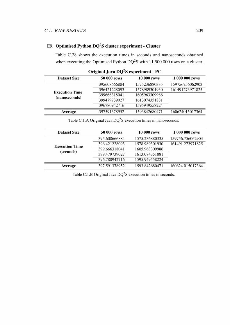
C.1. RAW RESULTS 209
E9. Optimised Python DQ2S cluster experiment - Cluster
Table C.28 shows the execution times in seconds and nanoseconds obtainedwhen executing the Optimised Python DQ2S with 11 500 000 rows on a cluster.
Original Java DQ2S experiment - PCDataset Size 50 000 rows 10 000 rows 1 000 000 rows
Execution Time(nanoseconds)
395608666884 1575236880335 159756756062903396421228093 1578989301930 161491273971825399666318041 1605963309986399479739027 1613074351881396780942716 1595949558224
Average 397591378952 1593842680471 160624015017364
Table C.1.A Original Java DQ2S execution times in nanoseconds.
Dataset Size 50 000 rows 10 000 rows 1 000 000 rows
Execution Time(seconds)
395.608666884 1575.236880335 159756.756062903396.421228093 1578.989301930 161491.273971825399.666318041 1605.963309986399.479739027 1613.074351881396.780942716 1595.949558224
Average 397.591378952 1593.842680471 160624.015017364
Table C.1.B Original Java DQ2S execution times in seconds.
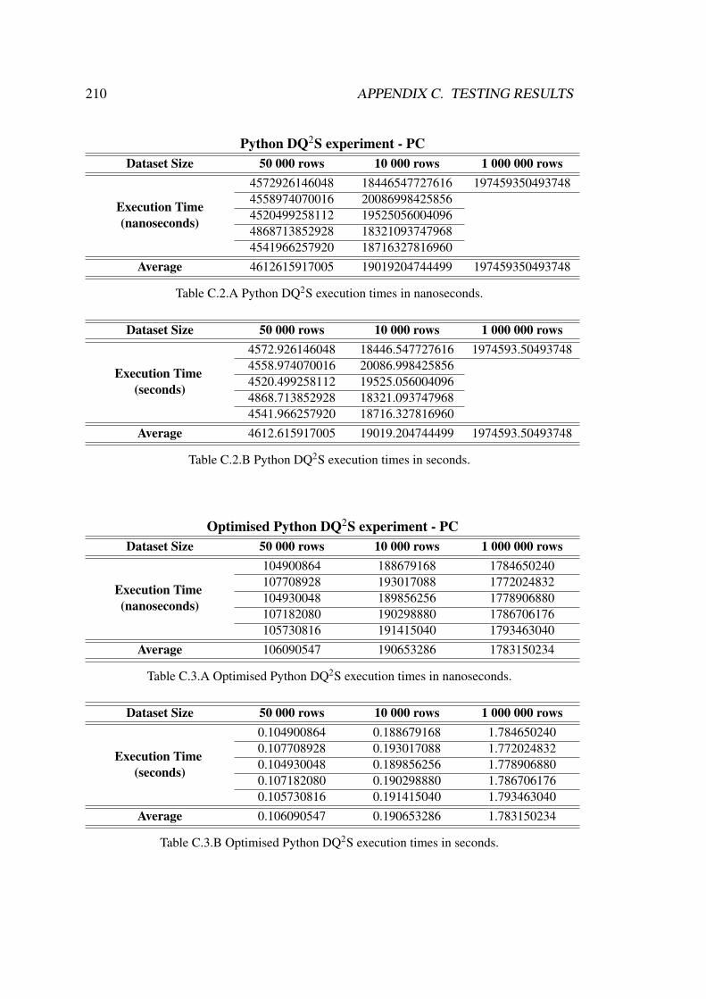
210 APPENDIX C. TESTING RESULTS
Python DQ2S experiment - PCDataset Size 50 000 rows 10 000 rows 1 000 000 rows
Execution Time(nanoseconds)
4572926146048 18446547727616 1974593504937484558974070016 200869984258564520499258112 195250560040964868713852928 183210937479684541966257920 18716327816960
Average 4612615917005 19019204744499 197459350493748
Table C.2.A Python DQ2S execution times in nanoseconds.
Dataset Size 50 000 rows 10 000 rows 1 000 000 rows
Execution Time(seconds)
4572.926146048 18446.547727616 1974593.504937484558.974070016 20086.9984258564520.499258112 19525.0560040964868.713852928 18321.0937479684541.966257920 18716.327816960
Average 4612.615917005 19019.204744499 1974593.50493748
Table C.2.B Python DQ2S execution times in seconds.
Optimised Python DQ2S experiment - PCDataset Size 50 000 rows 10 000 rows 1 000 000 rows
Execution Time(nanoseconds)
104900864 188679168 1784650240107708928 193017088 1772024832104930048 189856256 1778906880107182080 190298880 1786706176105730816 191415040 1793463040
Average 106090547 190653286 1783150234
Table C.3.A Optimised Python DQ2S execution times in nanoseconds.
Dataset Size 50 000 rows 10 000 rows 1 000 000 rows
Execution Time(seconds)
0.104900864 0.188679168 1.7846502400.107708928 0.193017088 1.7720248320.104930048 0.189856256 1.7789068800.107182080 0.190298880 1.7867061760.105730816 0.191415040 1.793463040
Average 0.106090547 0.190653286 1.783150234
Table C.3.B Optimised Python DQ2S execution times in seconds.

C.1. RAW RESULTS 211
Optimised Python DQ2S maximum capacity experiment - PCExecution Time nanoseconds seconds
Execution Time(11 500 000 rows)
21291235840 21.29123584021564015872 21.56401587221319143936 21.31914393621351192832 21.35119283221205413632 21.205413632
Average 21346200422 21.346200422
Table C.4: Optimised Python DQ2S execution times in nanoseconds and seconds for11 500 000 rows.
PySpark DQ2S Standalone mode in single machine - 1W1CDataset Size 50 000 rows 10 000 rows 1 000 000 rows
Execution Time(nanoseconds)
10662479104 11138216960 2072965683210515385088 11112353024 2070953523210487711744 11247056128 2071503897610559790080 11291499008 2087327897610610558208 11187699968 20823687168
Average 10567184845 11195365018 20770239437
Table C.5.A Execution times in nanoseconds obtained from PySpark DQ2S Standalone modein a single machine over 1 worker and 1 core.
Dataset Size 50 000 rows 10 000 rows 1 000 000 rows
Execution Time(seconds)
10.662479104 11.138216960 20.72965683210.515385088 11.112353024 20.70953523210.487711744 11.247056128 20.71503897610.559790080 11.291499008 20.87327897610.610558208 11.187699968 20.823687168
Average 10.567184845 11.195365018 20.770239437
Table C.5.B Execution times in seconds obtained from PySpark DQ2S Standalone mode in asingle machine over over 1 worker and 1 core.

212 APPENDIX C. TESTING RESULTS
PySpark DQ2S Standalone mode in single machine - 1W2CDataset Size 50 000 rows 10 000 rows 1 000 000 rows
Execution Time(nanoseconds)
8156534016 8737822976 146198530568256544768 8716681984 146290608648372070144 8642941952 145126300168278275840 8684564992 143659719688360314880 8824982784 14301459968
Average 8284747930 8721398938 14485795174
Table C.6.A Execution times in nanoseconds obtained from PySpark DQ2S Standalone modein a single machine over 1 worker and 2 cores each one.
Dataset Size 50 000 rows 10 000 rows 1 000 000 rows
Execution Time(seconds)
8.156534016 8.737822976 14.6198530568.256544768 8.716681984 14.6290608648.372070144 8.642941952 14.5126300168.278275840 8.684564992 14.3659719688.360314880 8.824982784 14.301459968
Average 8.284747930 8.721398938 14.485795174
Table C.6.B Execution times in seconds obtained from PySpark DQ2S Standalone mode in asingle machine over 1 worker and 2 cores each one.
PySpark DQ2S Standalone mode in single machine - 1W3CDataset Size 50 000 rows 10 000 rows 1 000 000 rows
Execution Time(nanoseconds)
7745988864 7973724928 127262208007787958016 7960871936 124218877447811255040 7848456960 122904816647710612992 7957158144 122228528647812652032 7915779840 12260795136
Average 7773693389 7931198362 12384447642
Table C.7.A Execution times in nanoseconds obtained from PySpark DQ2S Standalone modein a single machine over 1 worker and 3 cores each one.
Dataset Size 50 000 rows 10 000 rows 1 000 000 rows
Execution Time(seconds)
7.745988864 7.973724928 12.7262208007.787958016 7.960871936 12.4218877447.811255040 7.848456960 12.2904816647.710612992 7.957158144 12.2228528647.812652032 7.915779840 12.260795136
Average 7.773693389 7.931198362 12.384447642
Table C.7.B Execution times in seconds obtained from PySpark DQ2S Standalone mode in asingle machine over 1 worker and 3 cores each one.
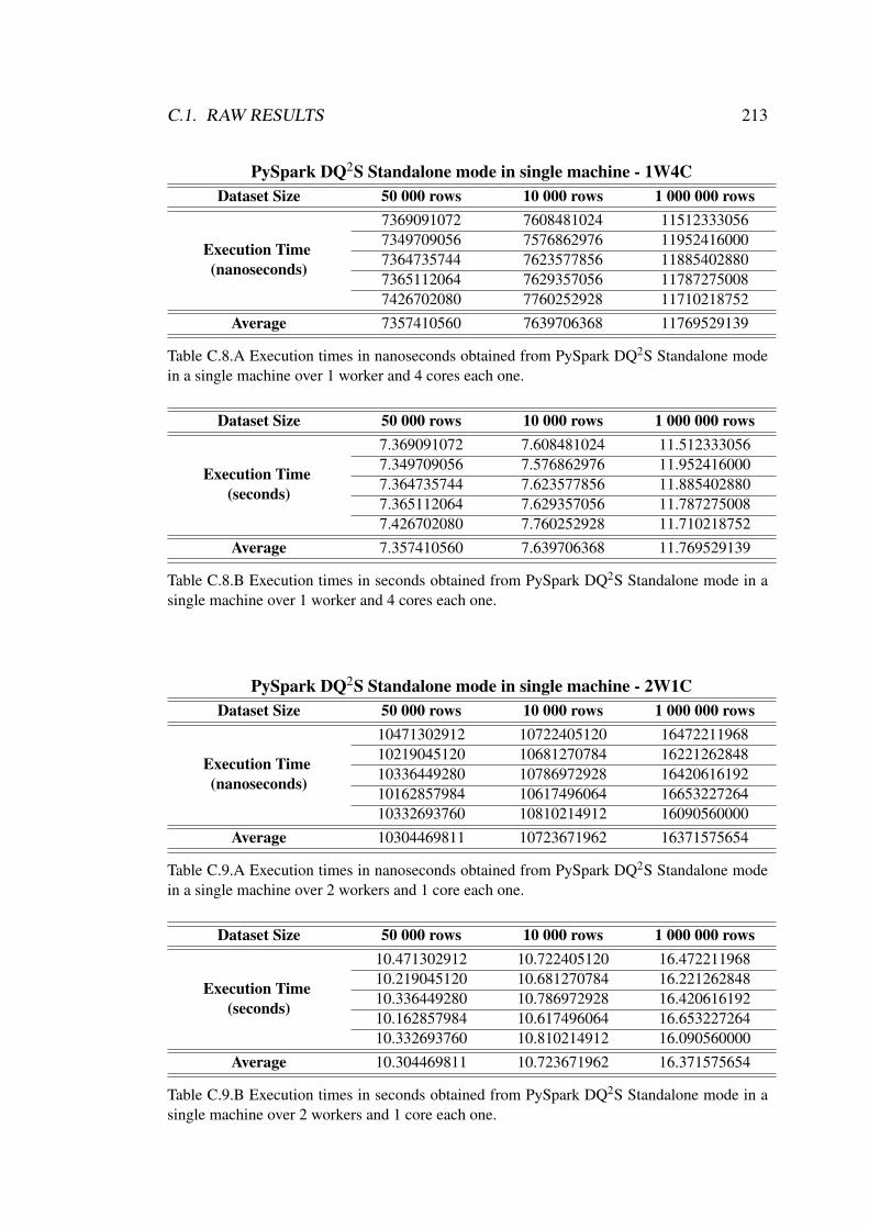
C.1. RAW RESULTS 213
PySpark DQ2S Standalone mode in single machine - 1W4CDataset Size 50 000 rows 10 000 rows 1 000 000 rows
Execution Time(nanoseconds)
7369091072 7608481024 115123330567349709056 7576862976 119524160007364735744 7623577856 118854028807365112064 7629357056 117872750087426702080 7760252928 11710218752
Average 7357410560 7639706368 11769529139
Table C.8.A Execution times in nanoseconds obtained from PySpark DQ2S Standalone modein a single machine over 1 worker and 4 cores each one.
Dataset Size 50 000 rows 10 000 rows 1 000 000 rows
Execution Time(seconds)
7.369091072 7.608481024 11.5123330567.349709056 7.576862976 11.9524160007.364735744 7.623577856 11.8854028807.365112064 7.629357056 11.7872750087.426702080 7.760252928 11.710218752
Average 7.357410560 7.639706368 11.769529139
Table C.8.B Execution times in seconds obtained from PySpark DQ2S Standalone mode in asingle machine over 1 worker and 4 cores each one.
PySpark DQ2S Standalone mode in single machine - 2W1CDataset Size 50 000 rows 10 000 rows 1 000 000 rows
Execution Time(nanoseconds)
10471302912 10722405120 1647221196810219045120 10681270784 1622126284810336449280 10786972928 1642061619210162857984 10617496064 1665322726410332693760 10810214912 16090560000
Average 10304469811 10723671962 16371575654
Table C.9.A Execution times in nanoseconds obtained from PySpark DQ2S Standalone modein a single machine over 2 workers and 1 core each one.
Dataset Size 50 000 rows 10 000 rows 1 000 000 rows
Execution Time(seconds)
10.471302912 10.722405120 16.47221196810.219045120 10.681270784 16.22126284810.336449280 10.786972928 16.42061619210.162857984 10.617496064 16.65322726410.332693760 10.810214912 16.090560000
Average 10.304469811 10.723671962 16.371575654
Table C.9.B Execution times in seconds obtained from PySpark DQ2S Standalone mode in asingle machine over 2 workers and 1 core each one.

214 APPENDIX C. TESTING RESULTS
PySpark DQ2S Standalone mode in single machine - 2W2CDataset Size 50 000 rows 10 000 rows 1 000 000 rows
Execution Time(nanoseconds)
9165194240 9250158080 134570618889152016128 9428869120 135122590729085235712 9415583744 132502087689009185792 9312792064 134690667529051820800 9383379968 13320818944
Average 9092690534 9358156595 13401883085
Table C.10.A Execution times in nanoseconds obtained from PySpark DQ2S Standalone modein a single machine over 2 workers and 2 cores each one.
Dataset Size 50 000 rows 10 000 rows 1 000 000 rows
Execution Time(seconds)
9.165194240 9.250158080 13.4570618889.152016128 9.428869120 13.5122590729.085235712 9.415583744 13.2502087689.009185792 9.312792064 13.4690667529.051820800 9.383379968 13.320818944
Average 9.092690534 9.358156595 13.401883085
Table C.10.B Execution times in seconds obtained from PySpark DQ2S Standalone mode in asingle machine over 2 workers and 2 cores each one.
PySpark DQ2S Standalone mode in single machine - 3W1CDataset Size 50 000 rows 10 000 rows 1 000 000 rows
Execution Time(nanoseconds)
10721553920 11476656896 1578769075210942905088 11374004992 1577969510410598299904 11213497088 1603183001610985516032 11401945856 1573194291210821647872 11572036096 15983724800
Average 10813984563 11407628186 15862976717
Table C.11.A Execution times in nanoseconds obtained from PySpark DQ2S Standalone modein a single machine over 3 workers and 1 core each one.
Dataset Size 50 000 rows 10 000 rows 1 000 000 rows
Execution Time(seconds)
10.721553920 11.476656896 15.78769075210.942905088 11.374004992 15.77969510410.598299904 11.213497088 16.03183001610.985516032 11.401945856 15.73194291210.821647872 11.572036096 15.983724800
Average 10.813984563 11.407628186 15.862976717
Table C.11.B Execution times in seconds obtained from PySpark DQ2S Standalone mode in asingle machine over 3 workers and 1 core each one.
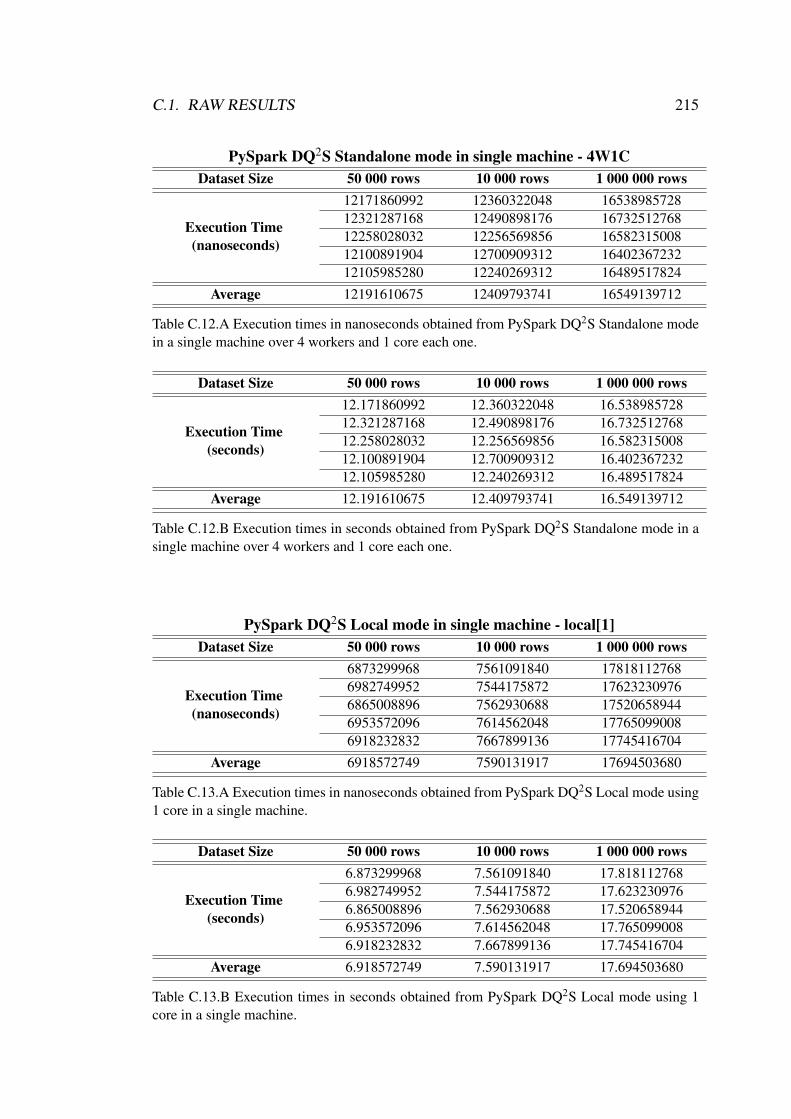
C.1. RAW RESULTS 215
PySpark DQ2S Standalone mode in single machine - 4W1CDataset Size 50 000 rows 10 000 rows 1 000 000 rows
Execution Time(nanoseconds)
12171860992 12360322048 1653898572812321287168 12490898176 1673251276812258028032 12256569856 1658231500812100891904 12700909312 1640236723212105985280 12240269312 16489517824
Average 12191610675 12409793741 16549139712
Table C.12.A Execution times in nanoseconds obtained from PySpark DQ2S Standalone modein a single machine over 4 workers and 1 core each one.
Dataset Size 50 000 rows 10 000 rows 1 000 000 rows
Execution Time(seconds)
12.171860992 12.360322048 16.53898572812.321287168 12.490898176 16.73251276812.258028032 12.256569856 16.58231500812.100891904 12.700909312 16.40236723212.105985280 12.240269312 16.489517824
Average 12.191610675 12.409793741 16.549139712
Table C.12.B Execution times in seconds obtained from PySpark DQ2S Standalone mode in asingle machine over 4 workers and 1 core each one.
PySpark DQ2S Local mode in single machine - local[1]Dataset Size 50 000 rows 10 000 rows 1 000 000 rows
Execution Time(nanoseconds)
6873299968 7561091840 178181127686982749952 7544175872 176232309766865008896 7562930688 175206589446953572096 7614562048 177650990086918232832 7667899136 17745416704
Average 6918572749 7590131917 17694503680
Table C.13.A Execution times in nanoseconds obtained from PySpark DQ2S Local mode using1 core in a single machine.
Dataset Size 50 000 rows 10 000 rows 1 000 000 rows
Execution Time(seconds)
6.873299968 7.561091840 17.8181127686.982749952 7.544175872 17.6232309766.865008896 7.562930688 17.5206589446.953572096 7.614562048 17.7650990086.918232832 7.667899136 17.745416704
Average 6.918572749 7.590131917 17.694503680
Table C.13.B Execution times in seconds obtained from PySpark DQ2S Local mode using 1core in a single machine.

216 APPENDIX C. TESTING RESULTS
PySpark DQ2S Local mode in single machine - local[2]Dataset Size 50 000 rows 10 000 rows 1 000 000 rows
Execution Time(nanoseconds)
5452984064 5802834944 115430172165412961792 5836121856 116203202565533444096 5890358784 117737349125526856704 5944324096 118859648005458756864 5752052224 11763933184
Average 5477000704 5845138381 11717394074
Table C.14.A Execution times in nanoseconds obtained from PySpark DQ2S Local mode using2 cores in a single machine.
Dataset Size 50 000 rows 10 000 rows 1 000 000 rows
Execution Time(seconds)
5.452984064 5.802834944 11.5430172165.412961792 5.836121856 11.6203202565.533444096 5.890358784 11.7737349125.526856704 5.944324096 11.8859648005.458756864 5.752052224 11.763933184
Average 5.477000704 5.845138381 11.717394074
Table C.14.B Execution times in seconds obtained from PySpark DQ2S Local mode using 2cores in a single machine.
PySpark DQ2S Local mode in single machine - local[3]Dataset Size 50 000 rows 10 000 rows 1 000 000 rows
Execution Time(nanoseconds)
5007549184 5338375936 108723092485062174208 5324840960 98712829445073466112 5298850048 100217390085012833280 5360150272 103051461125049060096 5317010688 10293234176
Average 5041016576 5327845581 10272742298
Table C.15.A Execution times in nanoseconds obtained from PySpark DQ2S Local mode using3 cores in a single machine.
Dataset Size 50 000 rows 10 000 rows 1 000 000 rows
Execution Time(seconds)
5.007549184 5.338375936 10.8723092485.062174208 5.324840960 9.8712829445.073466112 5.298850048 10.0217390085.012833280 5.360150272 10.3051461125.049060096 5.317010688 10.293234176
Average 5.041016576 5.327845581 10.272742298
Table C.15.B Execution times in seconds obtained from PySpark DQ2S Local mode using 3cores in a single machine.

C.1. RAW RESULTS 217
PySpark DQ2S Local mode in single machine - local[4]Dataset Size 50 000 rows 10 000 rows 1 000 000 rows
Execution Time(nanoseconds)
4945903104 5133988096 89704747524948933120 5181114112 87930119684965520896 5096628992 90888450564910916864 5260722688 87025459204972674048 5172325120 8819279872
Average 4948789606 5168955802 8874831514
Table C.16.A Execution times in nanoseconds obtained from PySpark DQ2S Local mode using4 cores in a single machine.
Dataset Size 50 000 rows 10 000 rows 1 000 000 rows
Execution Time(seconds)
4.945903104 5.133988096 8.9704747524.948933120 5.181114112 8.7930119684.965520896 5.096628992 9.0888450564.910916864 5.260722688 8.7025459204.972674048 5.172325120 8.819279872
Average 4.948789606 5.168955802 8.874831514
Table C.16.B Execution times in seconds obtained from PySpark DQ2S Local mode using 4cores in a single machine.

218 APPENDIX C. TESTING RESULTS
PySpark DQ2S Local mode in single machine - local[5]Dataset Size 50 000 rows 10 000 rows 1 000 000 rows
Execution Time(nanoseconds)
5198445056 5483340032 89174950405130334720 5582700032 89689351685182439936 5432392960 88969779205116220928 5463419136 90137679365130665984 5461233152 8936705792
Average 5151621325 5484617062 8946776371
Table C.17.A Execution times in nanoseconds obtained from PySpark DQ2S Local mode using5 cores in a single machine.
Dataset Size 50 000 rows 10 000 rows 1 000 000 rows
Execution Time(seconds)
5.198445056 5.483340032 8.9174950405.130334720 5.582700032 8.9689351685.182439936 5.432392960 8.8969779205.116220928 5.463419136 9.0137679365.130665984 5.461233152 8.936705792
Average 5.151621325 5.484617062 8.946776371
Table C.17.B Execution times in seconds obtained from PySpark DQ2S Local mode using 5cores in a single machine.
PySpark DQ2S Local mode in single machine - local[6]Dataset Size 50 000 rows 10 000 rows 1 000 000 rows
Execution Time(nanoseconds)
4805391104 5094859776 88353840644737410304 5095909888 87896558084778916096 5063123712 89251553284782843904 5035049984 88589921284723966976 5088356864 8657932032
Average 4765705677 5075460045 8813423872
Table C.18.A Execution times in nanoseconds obtained from PySpark DQ2S Local mode using6 cores in a single machine.
Dataset Size 50 000 rows 10 000 rows 1 000 000 rows
Execution Time(seconds)
4.805391104 5.094859776 8.8353840644.737410304 5.095909888 8.7896558084.778916096 5.063123712 8.9251553284.782843904 5.035049984 8.8589921284.723966976 5.088356864 8.657932032
Average 4.765705677 5.075460045 8.813423872
Table C.18.B Execution times in seconds obtained from PySpark DQ2S Local mode using 6cores in a single machine.

C.1. RAW RESULTS 219
PySpark DQ2S Local mode in single machine - local[7]Dataset Size 50 000 rows 10 000 rows 1 000 000 rows
Execution Time(nanoseconds)
4663134208 5044144896 87204569604644529920 5018700032 88789977604660646144 4997775104 86122831364693438976 5099013120 87106278404659883008 5034482176 8714520064
Average 4664326451 5038823066 8727377152
Table C.19.A Execution times in nanoseconds obtained from PySpark DQ2S Local mode using7 cores in a single machine.
Dataset Size 50 000 rows 10 000 rows 1 000 000 rows
Execution Time(seconds)
4.663134208 5.044144896 8.7204569604.644529920 5.018700032 8.8789977604.660646144 4.997775104 8.6122831364.693438976 5.099013120 8.7106278404.659883008 5.034482176 8.714520064
Average 4.664326451 5.038823066 8.727377152
Table C.19.B Execution times in seconds obtained from PySpark DQ2S Local mode using 7cores in a single machine.
PySpark DQ2S Local mode in single machine - local[8]Dataset Size 50 000 rows 10 000 rows 1 000 000 rows
Execution Time(nanoseconds)
4607827200 4969145088 90881249284634355712 4985406976 90996510724603010816 5042586112 95329889284640083968 5011299840 95068477444615563776 4959327744 9632914944
Average 4620168294 4993553152 9372105523
Table C.20.A Execution times in nanoseconds obtained from PySpark DQ2S Local mode using8 cores in a single machine.
Dataset Size 50 000 rows 10 000 rows 1 000 000 rows
Execution Time(seconds)
4.607827200 4.969145088 9.0881249284.634355712 4.985406976 9.0996510724.603010816 5.042586112 9.5329889284.640083968 5.011299840 9.5068477444.615563776 4.959327744 9.632914944
Average 4.620168294 4.993553152 9.372105523
Table C.20.B Execution times in seconds obtained from PySpark DQ2S Local mode using 8cores in a single machine.

220 APPENDIX C. TESTING RESULTS
PySpark DQ2S Local mode maximum capacity - local[1-6]Local[n] Local[1] Local[2] Local[3] Local[4] Local[5] Local[6]
Execution Time11 500 000 rows(nanoseconds)
131589269248 73765188096 60758119936 50822084096 47598737920 45034638080132989597184 74588361984 59746373888 50732338176 47743496960 44813570048132248972800 75507758080 57879614976 50409220096 46633732864 45086447872132390486016 75173811968 60409650944 49736065024 47446155264 44683708928132176488192 77783117824 57602428160 50325387776 46446733824 44617302016
Average 132278962688 75363647590 59279237581 50405019034 47173771366 44847133389
Table C.21.A Execution times in nanoseconds obtained from PySpark DQ2S Local mode using1 to 6 cores in a single machine for 11 500 000 rows.
Local[n] Local[1] Local[2] Local[3] Local[4] Local[5] Local[6]
Execution Time11 500 000 rows
(seconds)
131.589269248 73.765188096 60.758119936 50.822084096 47.598737920 45.034638080132.989597184 74.588361984 59.746373888 50.732338176 47.743496960 44.813570048132.248972800 75.507758080 57.879614976 50.409220096 46.633732864 45.086447872132.390486016 75.173811968 60.409650944 49.736065024 47.446155264 44.683708928132.176488192 77.783117824 57.602428160 50.325387776 46.446733824 44.617302016
Average 132.278962688 75.363647590 59.279237581 50.405019034 47.173771366 44.847133389
Table C.21.B Execution times in seconds obtained from PySpark DQ2S Local mode using 1 to6 cores in a single machine for 11 500 000 rows.
PySpark DQ2S Local mode maximum capacity - local[7-10, 12, 16]Local[n] Local[7] Local[8] Local[9] Local[10] Local[12] Local[16]
Execution Time11 500 000 rows(nanoseconds)
43831034880 43774910976 44017587968 44877532928 44712393984 4503220377644153880832 43759703040 44573113088 44557452800 44439171840 4502331494443686841856 43747205120 44671670784 44533266944 44352089088 4506173184043850480896 43493809920 44465067264 44111450880 44247652096 4442886092843825918208 43778395136 44287411968 44095034112 44282157824 44647308032
Average 43869631334 43710804838 44402970214 44434947533 44406692966 44838683904
Table C.22.A Execution times in nanoseconds obtained from PySpark DQ2S Local mode using7 to 10, 12, and 16 cores in a single machine for 11 500 000 rows.
Local[n] Local[7] Local[8] Local[9] Local[10] Local[12] Local[16]
Execution Time11 500 000 rows
(seconds)
43.831034880 43.774910976 44.017587968 44.877532928 44.712393984 45.03220377644.153880832 43.759703040 44.573113088 44.557452800 44.439171840 45.02331494443.686841856 43.747205120 44.671670784 44.533266944 44.352089088 45.06173184043.850480896 43.493809920 44.465067264 44.111450880 44.247652096 44.42886092843.825918208 43.778395136 44.287411968 44.095034112 44.282157824 44.647308032
Average 43.869631334 43.710804838 44.402970214 44.434947533 44.406692966 44.838683904
Table C.22.B Execution times in seconds obtained from PySpark DQ2S Local mode using 7 to10, 12, and 16 cores in a single machine for 11 500 000 rows.

C.1. RAW RESULTS 221
PySpark DQ2S Local mode maximum capacity - local[1-6]Local[n] Local[1] Local[2] Local[3] Local[4] Local[5] Local[6]
Execution Time35 000 000 rows(nanoseconds)
387859890944 226735009024 169449213184 144895914752 131416548864 125550755072389781254144 218828783872 170426714112 143335796992 131355746048 125424803840388898374912 219663964928 165627602944 143277867776 129674107904 125642475008386204375808 216963999232 181715121920 143071660800 130591193088 125979217920388046561792 222932421888 168523228928 143555652864 130743090944 126187362048
Average 388158091520 221024835789 171148376218 143627378637 130756137370 125756922778
Table C.23.A Execution times in nanoseconds obtained from PySpark DQ2S Local mode using1 to 6 cores in a single machine for 35 000 000 rows.
Local[n] Local[1] Local[2] Local[3] Local[4] Local[5] Local[6]
Execution Time35 000 000 rows
(seconds)
387.859890944 226.735009024 169.449213184 144.895914752 131.416548864 125.550755072389.781254144 218.828783872 170.426714112 143.335796992 131.355746048 125.424803840388.898374912 219.663964928 165.627602944 143.277867776 129.674107904 125.642475008386.204375808 216.963999232 181.715121920 143.071660800 130.591193088 125.979217920388.046561792 222.932421888 168.523228928 143.555652864 130.743090944 126.187362048
Average 388.158091520 221.024835789 171.148376218 143.627378637 130.756137370 125.756922778
Table C.23.B Execution times in seconds obtained from PySpark DQ2S Local mode using 1 to6 cores in a single machine for 35 000 000 rows.
PySpark DQ2S Local mode maximum capacity - local[7-10, 12, 16]Local[n] Local[7] Local[8] Local[9] Local[10] Local[12] Local[16]
Execution Time35 000 000 rows(nanoseconds)
123962601728 122784323072 123724978176 123729516032 124723767040 125474671872124133402112 123245732096 123591265792 124111967232 125511417856 125606431232123390970112 122825708288 123921627904 123391556864 123777323008 125879318016123952249856 123730597120 123490130944 123591343104 123716641792 124061688064124827040000 123664524800 123487019008 123417480192 123880696832 125312521984
Average 124053252762 123250177075 123643004365 123648372685 124321969306 125266926234
Table C.24.A Execution times in nanoseconds obtained from PySpark DQ2S Local mode using7 to 10, 12, and 16 cores in a single machine for 35 000 000 rows.
Local[n] Local[7] Local[8] Local[9] Local[10] Local[12] Local[16]
Execution Time35 000 000 rows
(seconds)
123.962601728 122.784323072 123.724978176 123.729516032 124.723767040 125.474671872124.133402112 123.245732096 123.591265792 124.111967232 125.511417856 125.606431232123.390970112 122.825708288 123.921627904 123.391556864 123.777323008 125.879318016123.952249856 123.730597120 123.490130944 123.591343104 123.716641792 124.061688064124.827040000 123.664524800 123.487019008 123.417480192 123.880696832 125.312521984
Average 124.053252762 123.250177075 123.643004365 123.648372685 124.321969306 125.266926234
Table C.24.B Execution times in seconds obtained from PySpark DQ2S Local mode using 7 to10, 12, and 16 cores in a single machine for 35 000 000 rows.

222 APPENDIX C. TESTING RESULTS
PySpark DQ2S Standalone mode on a cluster - 35 000 000 rowsNumber of worker nodes 1 2 3 4
Execution Time35 000 000 rows(nanoseconds)
66954494208 40034502144 36861419008 2967774387271653293056 40291827968 31768627968 2899857356874397865216 39341289984 31986951936 2824947097677074788864 39420195072 32379415040 2811791411273011555840 39189282816 33078972160 28194881024
Average 72618399437 39655419597 33215077222 28647716710
Table C.25.A Execution times in nanoseconds obtained from PySpark DQ2S Standalone modeprocessing 35 000 000 rows with 1 to 4 worker nodes on a cluster.
Number of worker nodes 1 2 3 4
Execution Time35 000 000 rows
(seconds)
66954494208 40.034502144 36.861419008 29.67774387271.653293056 40.291827968 31.768627968 28.99857356874.397865216 39.341289984 31.986951936 28.24947097677.074788864 39.420195072 32.379415040 28.11791411273.011555840 39.189282816 33.078972160 28.194881024
Average 72.618399437 39.655419597 33.215077222 28.647716710
Table C.25.B Execution times in seconds obtained from PySpark DQ2S Standalone mode pro-cessing 35 000 000 rows with 1 to 4 worker nodes on a cluster.
PySpark DQ2S Standalone mode on a cluster - 70 000 000 rowsNumber of worker nodes 1 2 3 4
Execution Time70 000 000 rows(nanoseconds)
101095668992 68086117888 54591626240 48209958144134146179072 66611641856 57330426880 49384262912104077149184 67483824896 58199030272 45521409024105101277184 70298240000 58156339200 44144183040131581689088 70488784896 54432688896 42770220032
Average 115200392704 68593721907 56542022298 46006006630
Table C.26.A Execution times in nanoseconds obtained from PySpark DQ2S Standalone modeprocessing 70 000 000 rows with 1 to 4 worker nodes on a cluster.
Number of worker nodes 1 2 3 4
Execution Time70 000 000 rows
(seconds)
101.095668992 68.086117888 54.591626240 48.209958144134.146179072 66.611641856 57.330426880 49.384262912104.077149184 67.483824896 58.199030272 45.521409024105.101277184 70.298240000 58.156339200 44.144183040131.581689088 70.488784896 54.432688896 42.770220032
Average 115.200392704 68.593721907 56.542022298 46.006006630
Table C.26.B Execution times in seconds obtained from PySpark DQ2S Standalone mode pro-cessing 70 000 000 rows with 1 to 4 worker nodes on a cluster.

C.1. RAW RESULTS 223
PySpark DQ2S Standalone mode on a cluster - 105 000 000 rowsNumber of worker nodes 1 2 3 4
Execution Time105 000 000 rows
(nanoseconds)
157113010176 88414319104 78251291136 60394453248144317761024 85405874176 73566785792 63932439040141386390784 87008677120 73601081088 55310124032142545898752 87754412288 73675163136 55662246912143911621888 83437327104 77529550080 57748296960
Average 145854936525 86404121958 75324774246 58609512038
Table C.27.A Execution times in nanoseconds obtained from PySpark DQ2S Standalone modeprocessing 105 000 000 rows with 1 to 4 worker nodes on a cluster.
Number of worker nodes 1 2 3 4
Execution Time105 000 000 rows
(seconds)
157.113010176 88.414319104 78.251291136 60.394453248144.317761024 85.405874176 73.566785792 63.932439040141.386390784 87.008677120 73.601081088 55.310124032142.545898752 87.754412288 73.675163136 55.662246912143.911621888 83.437327104 77.529550080 57.748296960
Average 145.854936525 86.404121958 75.324774246 58.609512038
Table C.27.B Execution times in seconds obtained from PySpark DQ2S Standalone mode pro-cessing 105 000 000 rows with 1 to 4 worker nodes on a cluster.
Optimised Python DQ2S maximum capacity experiment - ClusterExecution Time nanoseconds seconds
Execution Time(35 000 000 rows)
82839184128 82.83918412884307152128 84.30715212882913083136 82.91308313682871251968 82.87125196883172557056 83.172557056
Average 83220645683 83.2206456832
Table C.28: Optimised Python DQ2S execution times in nanoseconds and seconds for35 000 000 rows.

224 APPENDIX C. TESTING RESULTS
C.2 Performance Metrics Results
This section presents different calculations with a nine-decimal precision measuredwith the average runtime obtained from the tables above. All the labels from the tablesare correspondent to the formulas (4.1) to (4.5), explained in Section 4.6.1.
Table C.29 shows the performance metrics calculated using the information fromthe processing of 11 500 000 rows with the PySpark in Local mode, implemented ina single machine. The serial runtime (TS) is the runtime obtained from the OptimisedPython, conforming the best sequential runtime known; Serial runtime with 1 core(T(1)) is the runtime obtained from the Local mode with local[1], the parallel runtime(TP) correspond to the runtimes obtained with the parametrisation with local[n], wheren is a number from 2 to 10, 12 and 16. The relative speedup (rtS), and relative efficiency(rtE) are calculated considering the runtimes from T(1), whereas the real speedup (rS)and real efficiency (rE), are calculated with the values from TS, to produce values withrespect to the best sequential time known.
Table C.30.A, shows the performance metrics calculated using the informationfrom the processing of 50 000 rows. In this case, the serial runtime (TS) is the run-time obtained from the Optimised Python with the same number of rows as input. TheSerial runtime with 1 core (T(1)), utilised to calculate the relative speedup (rtS) andrelative efficiency (rtS), is the parallel runtime (TP) obtained from 1 worker and 1 Corefor 50 000 rows, with default parameters from the PySpark DQ2S instance.
Tables C.30.B and C.30.C show the information in the same way as C.30.A, butusing its correspondent value for TS, T(1) and TP, based on the average runtimes ob-tained from 100 000 and 1 000 000 rows.
Tables C.31.A, C.31.B, and C.31.C show the performance metrics calculated forthe values obtained from the PySpark in Local mode, executed on a single machinewith 50 000, 100 000, and 1 000 000 rows as corresponds.
PySpark DQ2S Local mode in single machine (11 500 000 rows)
Numberof cores
TS T(1) TP rS rtS rE rtE
1 21.34620042 132.279 132.279 0.161373 1 0.161373 1
2 21.34620042 132.279 75.36365 0.283243 1.755209 0.141621 0.877605
3 21.34620042 132.279 59.27924 0.360096 2.231455 0.120032 0.743818
4 21.34620042 132.279 50.40502 0.423494 2.624321 0.105873 0.65608
5 21.34620042 132.279 47.17377 0.452501 2.804079 0.0905 0.560816
6 21.34620042 132.279 44.84713 0.475977 2.949552 0.079329 0.491592

C.2. PERFORMANCE METRICS RESULTS 225
7 21.34620042 132.279 43.86963 0.486583 3.015274 0.069512 0.430753
8 21.34620042 132.279 43.7108 0.488351 3.02623 0.061044 0.378279
9 21.34620042 132.279 44.40297 0.480738 2.979057 0.053415 0.331006
10 21.34620042 132.279 44.43495 0.480392 2.976913 0.048039 0.297691
12 21.34620042 132.279 44.40669 0.480698 2.978807 0.040058 0.248234
16 21.34620042 132.279 44.83868 0.476067 2.950108 0.029754 0.184382
Table C.29: Performance Metrics for Parallel Algorithms: Values calculated for11 500 000 rows processing from PySpark Local mode in single machine execution.
PySpark DQ2S Standalone mode in single machine (50 000 rows)W C p Mem TS T(1) TP rS rtS rE rtE
1
1 1
14G
0.106090547 10.567184845 10.567184845 0.010039623 1.000000000 0.010039623 1.0000000002 2 0.106090547 10.567184845 8.284747930 0.012805525 1.275498655 0.006402763 0.6377493283 3 0.106090547 10.567184845 7.773693389 0.013647380 1.359351896 0.004549127 0.4531172994 4 0.106090547 10.567184845 7.375070003 0.014385022 1.432825023 0.003596256 0.358206256
2 1 2 7G 0.106090547 10.567184845 10.304469811 0.010295585 1.025495250 0.005147793 0.5127476252 2 4 0.106090547 10.567184845 9.092690534 0.011667674 1.162162597 0.002916918 0.2905406493 1 3 4.7G 0.106090547 10.567184845 10.813984563 0.009810496 0.977177726 0.003270165 0.3257259094 1 4 3.5G 0.106090547 10.567184845 12.191610675 0.008701930 0.866758718 0.002175483 0.216689680
Table C.30.A Performance Metrics for Parallel Algorithms: Values calculated for 50 000rows processing from PySpark Standalone mode in single machine execution.
PySpark DQ2S Standalone mode in single machine (100 000 rows)W C p Mem TS T(1) TP rS rtS rE rtE
1
1 1
14G
0.190653286 11.195365018 11.195365018 0.017029662 1.000000000 0.017029662 1.0000000002 2 0.190653286 11.195365018 8.721398938 0.021860402 1.283666198 0.010930201 0.6418330993 3 0.190653286 11.195365018 7.931198362 0.024038396 1.411560335 0.008012799 0.4705201124 4 0.190653286 11.195365018 7.639706368 0.024955578 1.465418234 0.006238894 0.366354559
2 1 2 7G 0.190653286 11.195365018 10.723671962 0.017778732 1.043986151 0.008889366 0.5219930762 2 4 0.190653286 11.195365018 9.358156595 0.020372953 1.196321616 0.005093238 0.2990804043 1 3 4.7G 0.190653286 11.195365018 11.407628186 0.016712789 0.981392875 0.005570930 0.3271309584 1 4 3.5G 0.190653286 11.195365018 12.409793741 0.015363131 0.902139492 0.003840783 0.225534873
Table C.30.B Performance Metrics for Parallel Algorithms: Values calculated for100 000 rows processing from PySpark Standalone mode in single machine execution.
PySpark DQ2S Standalone mode in single machine (1 000 000 rows)W C p Mem TS T(1) TP rS rtS rE rtE
1
1 1
14G
1.783150234 20.770239437 20.770239437 0.085851212 1.000000000 0.085851212 1.0000000002 2 1.783150234 20.770239437 14.485795174 0.123096469 1.433834953 0.061548234 0.7169174763 3 1.783150234 20.770239437 12.384447642 0.143983025 1.677122794 0.047994342 0.5590409314 4 1.783150234 20.770239437 11.769529139 0.151505656 1.764746847 0.037876414 0.441186712
2 1 2 7G 1.783150234 20.770239437 16.371575654 0.108917448 1.268676875 0.054458724 0.6343384372 2 4 1.783150234 20.770239437 13.401883085 0.133052215 1.549800077 0.033263054 0.3874500193 1 3 4.7G 1.783150234 20.770239437 15.862976717 0.112409560 1.309353207 0.037469853 0.4364510694 1 4 3.5G 1.783150234 20.770239437 16.549139712 0.107748817 1.255064601 0.026937204 0.313766150
Table C.30.C Performance Metrics for Parallel Algorithms: Values calculated for 1 000 000rows processing from PySpark Standalone mode in single machine execution.

226 APPENDIX C. TESTING RESULTS
PySpark DQ2S Local mode in single machine (50 000 rows)Number of
cores TS T(1) TP rS rtS rE rtE
1 0.106090547 6.918572749 6.918572749 0.015334167 1.000000000 0.015334167 1.0000000002 0.106090547 6.918572749 5.477000704 0.019370190 1.263204648 0.009685095 0.6316023243 0.106090547 6.918572749 5.041016576 0.021045467 1.372455862 0.007015156 0.4574852874 0.106090547 6.918572749 4.948789606 0.021437676 1.398033317 0.005359419 0.349508329
Table C.31.A Performance Metrics for Parallel Algorithms: Values calculated for 50 000rows processing from PySpark Local mode in single machine execution.
PySpark DQ2S Local mode in single machine (100 000 rows)Number of
cores TS T(1) TP rS rtS rE rtE
1 0.190653286 7.590131917 7.590131917 0.025118573 1.000000000 0.025118573 1.0000000002 0.190653286 7.590131917 5.845138381 0.032617412 1.298537592 0.016308706 0.6492687963 0.190653286 7.590131917 5.327845581 0.035784312 1.424615598 0.011928104 0.4748718664 0.190653286 7.590131917 5.168955802 0.036884294 1.468407200 0.009221074 0.367101800
Table C.31.B Performance Metrics for Parallel Algorithms: Values calculated for100 000 rows processing from PySpark Local mode in single machine execution.
PySpark DQ2S Local mode in single machine (1 000 000 rows)Number of
cores TS T(1) TP rS rtS rE rtE
1 1.783150234 17.694503680 17.694503680 0.100774244 1.000000000 0.100774244 1.0000000002 1.783150234 17.694503680 11.717394074 0.152179761 1.510105709 0.076089881 0.7550528543 1.783150234 17.694503680 10.272742298 0.173580742 1.722471290 0.057860247 0.5741570974 1.783150234 17.694503680 8.874831514 0.200922151 1.993784744 0.050230538 0.498446186
Table C.31.C Performance Metrics for Parallel Algorithms: Values calculated for 1 000 000rows processing from PySpark Local mode in single machine execution.
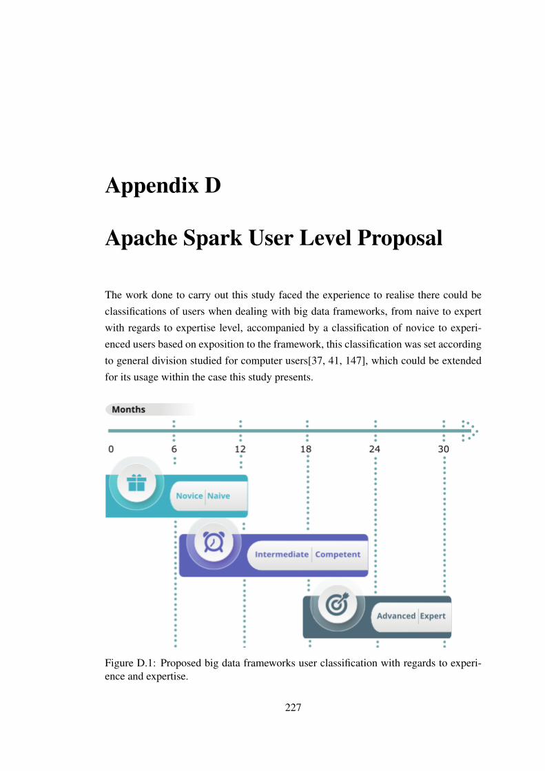
Appendix D
Apache Spark User Level Proposal
The work done to carry out this study faced the experience to realise there could beclassifications of users when dealing with big data frameworks, from naive to expertwith regards to expertise level, accompanied by a classification of novice to experi-enced users based on exposition to the framework, this classification was set accordingto general division studied for computer users[37, 41, 147], which could be extendedfor its usage within the case this study presents.
Figure D.1: Proposed big data frameworks user classification with regards to experi-ence and expertise.
227
228 APPENDIX D. APACHE SPARK USER LEVEL PROPOSAL
The user’s level of exposure can be classified on three: novice, intermediate andadvanced, assuming a quality exposure where the user was involved in gaining skillsand knowledge. Quality on the exposure is measured on a range of naive, competentand expert. With the designation mentioned, a novice user might have from 0 to 12months of exposure to the framework, with naive expertise; whereas an intermediateuser might have from 6 to 24 months of exposure and a competent expertise; advancedusers should have more than 24 months of exposure with a competent expertise, oraround 18 months with expert skills. The temporal classification proposed is repre-sented in Figure D.1. There is a larger gap between being competent and expert, andintermediate to advanced, than the gap from making a step out of being a naive, noviceuser, this is because once the basic elements are understood, the common tasks are suc-cessfully implemented, and the general knowledge is acquired, there is a wide path tospecialisation with big data frameworks; in Apache Spark, the users could be classifiedaccording to the following:
1. Novice and naive
• Basic knowledge of big data.
• Entry involvement on big data frameworks.
• Basic understanding of MapReduce paradigm.
• Capable of processing Apache Spark applications without any understand-ing of Spark’s processing model.
• Development of Spark applications without any built-in library.
• Unaware of the available parametrisation that can be done to Spark’s jobs.
• With little to zero involvement on community discussion forums.
• Able to provide answers to questions regarding Spark’s general character-istics.
• Unable to provide answers to general technical and low level questionsregarding Spark’s details.
• Unable to provide thorough answers to any question regarding Spark.
2. Intermediate and competent
• Knowledge about big data and one specialisation (quality, security, man-agement, visualisation, etc.).

229
• Familiar with the big data framework ecosystem.
• Competent understanding of MapReduce.
• Use of Apache Spark with knowledge on its internal processes, both onsoftware and hardware level.
• Clear knowledge of the elements involved in the processing of ApacheSpark.
• Capable of utilise at least one Spark built-in library, and general knowledgeabout the main libraries.
• Able to understand on high level Apache’s different modes and availablecluster managers.
• Able to configure and utilise at least one cluster manager.
• Aware of the parametrisation that can be done to Spark’s jobs.
• Able to set common parameters without in-depth understanding of its func-tion.
• Able to perform basic tuning to Spark’s jobs.
• Usually actively involved on community discussion forums.
• Able to provide answers to questions regarding Spark’s general character-istics with detail.
• Capable of providing answers to general technical questions regarding Spark.
• Able to provide thorough answers to some questions regarding Spark.
3. Advanced and expert
• Experience and knowledge on more than one big data framework.
• Strong knowledge on big data, and knowledge on more than one speciali-sation or strong knowledge on one.
• Solid understanding of MapReduce paradigm.
• Competent knowledge on Spark’s available libraries, and strong skills toutilise at least one.
• Able to configure and utilise more than one cluster manager.
• Able to integrate and utilise other open source projects with Spark.

230 APPENDIX D. APACHE SPARK USER LEVEL PROPOSAL
• Able to perform tuning to Spark’s jobs for different kinds of algorithms anduse cases.
• Actively involved on community discussion forums.
• Able to provide thoruanswers to questions regarding Spark’s general char-acteristics with detail.
• Able to provide thorough answers to a wide number of questions regardingSpark, from technical aspects to high level details.
Some users might already have expertise and involvement on big data frameworks,and an advantage on MapReduce and big data understanding if Hadoop was previ-ously known. The list above is not extensive and does not pretend to over generalise,considering that users could present different behaviours, backgrounds and levels ofexposure; each case could be hugely different but, this is a proposed high level clas-sification, comprising the basic elements each novice, intermediate and advanced bigdata framework user should consider.