arX

iv:1

704.

0035

1v1

[q-

bio.

QM

] 2

Apr

201

7

Two-exponential models of gene expression patterns for noisy

experimental data

Theodore Alexandrov 1,2,3, Nina Golyandina 4,∗,

David Holloway 5, Alex Shlemov 4 and Alexander Spirov 6,7

April 4, 2017

1EMBL Heidelberg, Meyerhofstr. 1, Heidelberg, 69117, Germany,2Skaggs School of Pharmacy and Pharmaceutical Sciences, University of California of San Diego, La Jolla, CA9500, USA,3SCiLS GmbH, Bremen, 28359, Germany,4St. Petersburg State University, Universitetskaya nab. 7/9, St.Petersburg, 199034, Russia,5Mathematics Department, British Columbia Institute of Technology, 3700 Willingdon Avenue, Burnaby, B.C.,V5G 3H2, Canada,6Computer Science and CEWIT, SUNY Stony Brook, 1500 Stony Brook Road, Stony Brook, NY 11794, USAand7The Sechenov Institute of Evolutionary Physiology & Biochemistry, Torez Pr. 44, St.Petersburg, 194223,Russia.∗ the corresponding author, nina@gistatgroup.com

Abstract

Motivation: Spatial pattern formation of the primary anterior-posterior morphogenetic gradient of thetranscription factor Bicoid (Bcd) has been studied experimentally and computationally for many years. Bcdspecifies positional information for the downstream segmentation genes, affecting the fly body plan. Morerecently, a number of researchers have focused on the patterning dynamics of the underlying bcd mRNAgradient, which is translated into Bcd protein. New, more accurate techniques for visualizing bcd mRNA needto be combined with quantitative signal extraction techniques to reconstruct the bcd mRNA distribution.Results: Here, we present a robust technique for quantifying gradients with a two-exponential model. Thisapproach: 1) has natural, biologically relevant parameters; and 2) is invariant to linear transformations ofthe data which can arise due to variation in experimental conditions (e.g. microscope settings, non-specificbackground signal). This allows us to quantify bcd mRNA gradient variability from embryo to embryo(important for studying the robustness of developmental regulatory networks); sort out atypical gradients;and classify embryos to developmental stage by quantitative gradient parameters.

1 Background

Biology A key concept in developmental biology is that of morphogen gradients (Briscoe et al., 2010),in which a spatially-distributed gradient of a signaling molecule (morphogen) affects downstream cellularresponses in a concentration-dependent manner. These spatial gradients are established by molecular trans-port, either active or diffusional. One of the best-studied morphogen gradients in development is of theprotein transcription factor Bicoid (Bcd) (Briscoe et al., 2010; Grimm et al., 2010), which regulates geneexpression along the anterior-posterior (AP) axis of the developing fruit fly (Drosophila) embryo. The Bcdprotein gradient has been studied quantitatively for many years, both in terms of quantitative experimentsand in mathematical modeling of the dynamics of gradient formation.

More recently, studies have focused on the underlying dynamics and patterning of the bcd mRNA gra-dient, since the Bcd protein forms via translation from the mRNA. The bcd RNA gradient forms earlierthan the protein gradient, and exhibits a number of distinct features from the protein pattern. Thesehave been the subject of several mathematical modeling projects, as well as new quantitative experimentalprojects to characterize the bcd mRNA gradient (Spirov et al., 2009; Lipshitz, 2009; Kavousanakis et al.,2010; Deng et al., 2010; Little et al., 2011; Cheung et al., 2011, 2014; Dalessi et al., 2012; Liu and Niranjan,2012; Fahmy et al., 2014; Ali-Murthy and Kornberg, 2016).

1

There are a number of features to bcd RNA patterning which make it more complex to study than theBcd protein pattern. These features require new and more sophisticated techniques in data acquisition andsignal processing in order to extract quantitative data. The current paper presents and validates a newmethod for quantitative analysis of spatial profiles of bcd RNA reliably extracted from whole embryo 3Dscans (confocal microscopy) of FISH (fluorescent in situ hybridization) RNA data.

Data Figure 1A shows a sagittal section through the middle of such a whole embryo scan, with fluores-cence intensity proportional to the concentration of bcd mRNA. The dataset is 3D, and the RNA transportsetting up this 3D pattern has components in the three coordinates: head-to-tail (AP); top-to-bottom(dorso-ventral, DV); and inside-to-outside (basal-apical, BA). The gradient is chiefly along the AP direction:biologically, the mRNA spreads posteriorly from a maternal deposition at the anterior end of the embryo.There are however, concentration differences in the DV direction, and while bcd RNA and protein patternsare most intense in the surface, or cortex, of the embryo, bcd is also found in the interior of the embryo, andthere is a concentration gradient in the BA direction. The transport processes establishing these gradientsmay differ between the different coordinates: AP transport of bcd RNA involves minus-end motors traffick-ing along microtubules, assisted by proteins such as Staufen (Stau) (Weil et al., 2006, 2008; Spirov et al.,2009; Fahmy et al., 2014; Ali-Murthy and Kornberg, 2016); DV ‘bending’ of bcd pattern may reflect geo-metric asymmetries in the embryo; and BA transport appears to occur at later stages of development, byan unknown mechanism (Bullock and Ish-Horowicz, 2001; Spirov et al., 2009; Fahmy et al., 2014).

Approach In whole embryo imaging, variability can arise during tissue fixation and staining with flu-orophores, as well as from differences in microscope settings (gain and offset) between measurements ofdifferent batches of embryos on different days. Here, we discuss features of the data extraction which areinsensitive to such experimental variation.

The aim of our approach is to create a model for basal and apical profiles (see Figure 1B) with bcd

gradients, estimate the model parameters and show that they can help to obtain biological results; inparticular, to compare different ages in the embryo development. We show an example of how data extractedand modelled by this technique can provide new biological insights into bcd RNA gradient formation.

The novelty of the approach consists in consideration of the model parameters, which do not dependon linear transformation of the data and thereby on the non-specific background signal and the microscopesettings. It is very important, since otherwise the comparison results can be caused by the experimentsconditions, not by the biology reasons.

Model A two-exponential fit of a Bcd protein profile can be well approximated by a single exponentialplus a nearly-constant background (Houchmandzadeh et al., 2002; Alexandrov et al., 2008). In contrast,while some bcd RNA profiles show such characteristics, many others, especially at early stages, show a muchsharper exponential drop in the anterior, plus a constant or even posteriorly-rising component through therest of the embryo (Figure 2). The transition between components can be readily visible in RNA patterns(and not in protein), as a ‘kink’ around the 20–30% egg length (%EL) position. These different componentssuggest multiple scales (or mechanisms) in the posterior-ward transport of bcd RNA.

Technique We previously applied a signal extraction technique based on Singular Spectrum Analysis(SSA) to quantify Bcd protein gradients (Alexandrov et al., 2008). This demonstrated that SSA couldreliably and automatically extract AP Bcd protein gradients. These were the sum of two exponentials, onewith a significant decay constant (strong curvature) and one of nearly linear form, capturing the non-specificbackground signal. Here, we adapt the SSA technique to the more complex cases of bcd RNA gradients,validating the reliability and effectiveness of the approach. SSA itself is used for signal extraction, and theSSA-related method ESPRIT (Roy and Kailath, 1989; Golyandina and Zhigljavsky, 2013) is used for theestimation of signal parameters.

SSA techniques have proven to be robust to signal extraction from data with substantial experimen-tal variability and intrinsic noise (Golyandina et al., 2001; Alexandrov et al., 2008; Alonso et al., 2005;Golyandina et al., 2012; Golyandina and Zhigljavsky, 2013). The use of SSA for extraction of signals ingene expression data was in Spirov et al. (2012); Golyandina et al. (2012); Shlemov et al. (2015a,b).

2

A

B

Figure 1: Preparation of data for quantitative analysis of sagittal images by 1D Singular Spectrum Analysis(SSA). A. Fluorescence intensity is proportional to the concentration of bcd RNA. The gradient in bcd mRNA ischiefly in the head-to-tail, AP, direction (left to right), but DV variation (top-to-bottom coordinate) can be seen,as well as variation by depth in the embryo (BA direction). For transport and patterning along the surface ofthe embryo, the natural coordinates are curvilinear. For extraction of the head-to-tail gradient patterning, thecurvilinear coordinates are well approximated by a projection onto the AP axis (see text). B. For quantificationof the AP gradient and BA differences, we sample data from an apical layer above the cortical nuclei and froma basal layer below the cortical nuclei, using chains of overlapping regions of interest (ROIs). Data from eachlayer is analyzed independently with 1D SSA. Each layer can then be plotted as intensity vs. AP position (rightinset).

3

A AP, %

0

50

100

150

20 40 60 80

profileESPRIT approxanterior expshallow expresiduals

B AP, %

0

50

100

20 40 60 80

profileESPRIT approxanterior expshallow expresiduals

C AP, %

0

50

100

20 40 60 80

profileESPRIT approxanterior expshallow expresiduals

D AP, %

0

50

100

20 40 60 80

profileESPRIT approxanterior expshallow expresiduals

Figure 2: Representative examples of AP profiles of bcd mRNA, illustrating the variety of cases and efficacy ofthe modeling approach. Blue is the original data, red is the ESPRIT fit, the sum of two exponentials (green andmagenta, individually). A. An early nuclear cleavage cycle 14A (nc14) embryo with a typical broad anteriorexponential (green) and shallow 2nd component (magenta) extending throughout the embryo (Cf Spirov et al.(2009)). B. A bcd mRNA profile in which the 2nd, trunk, component rises towards the posterior (i.e. has apositive exponential rate). C. A case with a nearly flat 2nd component (representing the mRNA signal posteriorof 25%EL). D. An embryo with a very sharp anterior (1st component) exponential, dropping to low values by10%EL.

4

2 Methods

2.1 Two-exponential modeling

We fit the following two-exponential function (of AP distance, x) to bcd mRNA data, to capture the distincttwo-component pattern of most bcd RNA gradients (with the ‘kink’, commonly observed at 20–30 %EL):

s(x) = Canterioreαanteriorx + Cshallowe

αshallowx, (1)

ors(x) = Canteriorλ

x

anterior + Cshallowλx

shallow,

for λ = eα. The two components, anterior (for the sharp, quickly decaying pattern in the anterior) andshallow (for the more constant component in the mid- and posterior embryo), each have two parameters -an amplitude C, and a decay λ. The anterior exponential is always decreasing and therefore λanterior < 1,αanterior < 0; while the shallow exponential can be decreasing or increasing (Figure 1). In biological terms,C for λ < 1 represents the maximum concentration of the component, and λ represents the rate at whichthe component decreases (or increases) along the AP coordinate.

One-exponential plus constant background is a special case of equation (1), with λshallow = 1 (or αshallow =0). Use of (1) does not require two strong (nonzero α) exponentials in the signal (pattern). In the case ofthe model commonly applied to the Bcd protein gradient, the first exponential describes the signal and thesecond exponential describes the non-specific background signal and the offset of the microscope.

Raw image data is likely of the form s(x)+ε(x), where ε(x) represents “noise”, i.e. non-regular oscillationswith zero mean.

2.1.1 Model characteristics independent of the microscopy gain/offset and background

To remove effects from variability in microscope settings (gain and offset) and the unknown form of non-specific background (Houchmandzadeh et al., 2002; Myasnikova et al., 2005; Holloway et al., 2006), gradientcharacteristics can be used which do not change under a linear transformation of the gradient.

That is, if each profile (gradient) can be represented by the linear transformation:

f(x) = A(s(x) + ε(x)) +B, (2)

where A and B represent an unknown scaling and an unknown offset, respectively. A and B are likelyto differ between embryos (with different staining conditions, microscope settings, etc.), but when we takebasal and apical traces within each embryo image, we assume that the A and B are constant within a singleembryo. To compare data between embryos, we take advantage of the independence of the following profilecharacteristics from linear transformations, i.e. independence from A and B values.

• the ratio between the anterior gradient pre-exponential coefficients for the apical and basal profilesCab = ln(Capical

anterior/Cbasalanterior) ;

• the following ratio for the shallow componentC

(apical)shallow α

(apical)shallow /(C

(basal)shallowα

(basal)shallow);

• indicators of non-increase in the shallow components λapicalshallow ≤ 1 and λbasal

shallow ≤ 1;

• in addition, the AP position at which the anterior components become almost zero AP0(apical)anterior and

AP0(basal)anterior.

These relations underlie the quantitative conclusions in this paper. We also use these relations to screenfor non-typical embryos, which aids in following the development of the bcd RNA gradient over time and forstudying apical-basal differences.

Mathematical details We will use index 1 for anterior and index 2 for shallow. The signal (1) hascharacteristics which approximately satisfy independency from linear transformations if the second (shallow-gradient) exponential rate is small enough (λ2≅1, α2≅0) and can therefore be approximated by a linearfunction. This is a reasonable assumption for the bcd mRNA data, giving

A(C1 exp(α1x) +C2 exp(α2x)) +B ≈

AC1 exp(α1x) + AC2(1 + α2x) +B ≈ C1 exp(α1x) + C2 exp(α2x),

where

C1 = AC1, α1 = α1, C2 = AC2 +B, α2 = AC2α2/(AC2 +B).

5

Thus, the following characteristics of the profiles can be considered as almost independent of a linear trans-formation of the intensities, i.e., of A and B:

α(apical)1 , C

(apical)2 α

(apical)2 /C

(apical)1 , (3)

α(basal)1 , C

(basal)2 α

(basal)2 /C

(basal)1 , (4)

C(apical)1 /C

(basal)1 , C

(apical)2 α

(apical)2 /(C

(basal)2 α

(basal)2 ), (5)

where (3) are characteristics of apical profiles, (4) are characteristics of basal profiles, and characteristics(5) show relations between apical and basal profiles. If C2 > 0 and AC2 + B > 0 (true, generally, for thebcd RNA data), the sign of α2 is not affected by a linear transformation and the second exponential can beeither increasing or decreasing.

2.1.2 Estimation of the two-exponential model parameters

We use the subspace-based method ESPRIT, motivated by the success of SSA (also a subspace-based method)in smoothing one-dimensional gene profiles from Drosophila embryos (Alonso et al., 2005; Golyandina et al.,2012). On profiles from different genes, the method proved to be robust to high noise and to variations inembryo characteristics.

The mathematical details of ESPRIT can be found in the Supplementary material. We use the methodto estimate the exponential decays in (1): λ

(apical)anterior, λ

(basal)anterior, λ

(apical)shallow and λ

(basal)shallow. The estimation of the

coefficients C(apical)anterior, C

(basal)anterior, C

(apical)shallow and C

(basal)shallow are then found by conventional least-squares, since the

model (1) is linear in these parameters.Since the first exponential is expected to be rapidly decreasing (λanterior < 1) and the second exponential

is expected to be close to constant (λshallow near 1), we reorder the ESPRIT estimates accordingly.

2.2 Data

2.2.1 FISH and data acquisition

Fluorescent in situ hybridization (FISH) for bcd mRNA is as described in Spirov et al. (2009), see the Supple-mentary materials for more details. Computational tools to process midsagittal images are described in theSupplementary Materials too. Our dataset consists of images of about 160 embryos, ranging in stage fromunfertilized eggs (not analyzed) to early nuclear cleavage cycle 14A (nc14, same dataset as in Spirov et al.(2009)). In the current study, we analyzed 124 embryos. These were divided into three developmentalstages, based on preliminary analysis and biological considerations: Cleavage, or pre-blastoderm (nc1–nc9);Syncytial Blastoderm (nc10–nc13); and Cellularizing Blastoderm (nc14A). The Cleavage stage is long, last-ing about 80 min (at room temperature), and has highly variable bcd mRNA gradients. For more detailedanalysis, we subdivided Cleavage into two sub-groups: Early (nc1–nc8) and Late (nc9). The SyncytialBlastoderm stage spans about 45 min, and this could be subdivided into two sub-groups: nc10–nc12 andnc13). The last stage, early nc14A, is short (15–20 min.), but highly variable and dynamic. Careful visualinspection allowed us to divide the nc14A embryos on three sub-groups: early, mid and late (Spirov et al.,2009).

2.2.2 Construction of 1D profiles

Raw data from the confocal microscope consists of mRNA intensities per a small circular area with 2Dspatial coordinates. After selecting the regions of interest (ROI chains), two techniques were tested forconverting the data into 1D AP profiles. The first (and simplest) technique projects intensities onto anAP axis orthogonal to the DV axis by discarding the DV component of the coordinate (Figure 1A). Thishas been used by many groups, see for example Surkova et al. (2008); Houchmandzadeh et al. (2002)). Thesecond technique preserves the natural curvilinear coordinates of the embryo, with distance between ROIscalculated by d2(i) = (AP(i+1)−AP(i))2+(DV(i+1)−DV(i))2. Cumulative distances are then normalizedby dividing by the sum of d(i).

Regardless of the technique (AP or curvilinear coordinates), the 1D coordinates obtained are not equidis-tant. Linear interpolation was used to create equidistant points of a given spatial step. A step 0.08–0.1%ELwas chosen to generate approximately equal numbers of points for the two techniques. These results obtainedby means of AP coordinates appear to be more precise than that obtained by curvilinear coordinates, seethe Supplementary material for comparison. Therefore, we can consider only AP coordinates in the paper.

6

3 Results and discussion

3.1 Model application

Figure 2 demonstrates a set of examples to illustrate the variety of profiles which can be fit by the two-exponential model. These include the typical profiles considered in Spirov et al. (2009), with a rapidlydecreasing anterior gradient and slowly decreasing gradient to the posterior (Figure 2A), and profiles withincreasing (Figure 2B) or flat (Figure 2C) posterior gradients.

Data is generally too biased and noisy from the terminal regions of the embryo: 0–10 %EL and 90–100%EL(Cf (Surkova et al., 2008; Houchmandzadeh et al., 2002), see Figure 2). Processing and analyzing datafrom 10–90 %EL is sufficient for extracting bcd RNA profiles from nearly all embryos older than nc6. Forvery early embryos (CleavageEarly stage), gradients have just begun to form from initial terminal locales;in these cases, we process from 5–93 %EL Figure 2D. Figure 2 shows that the two-exponential model suitsdifferent types of data very well.

Typically, embryos have a decreasing anterior exponential component and decreasing or close-to-constantshallow posterior gradients (both for the apical and basal profiles). We call these Type 1 (typical) embryos.Some embryos, however, show a posteriorly-increasing shallow gradient for either apical or basal profiles.We call these Type 2 (atypical) embryos. Type 2 profiles are common early in development (Cleavage) anduncommon in later stages. Here, we focus on Type 1 embryos, which represent the majority of the dataset.

Detection of Type 1 can be performed by means of exponential rates of the shallow exponents: (A)

λ(apical)shallow < 1.002, λ

(basal)shallow < 1.002. This condition screens for shallow profiles (both basal and apical) which

do not increase towards the posterior (1.002 is used for 1, to account for estimation errors).

3.2 Model validation

Even within one developmental stage, the shape of mRNA profiles from embryo to embryo is highly variable.This makes construction of a prototype profile challenging, and complicates understanding of the underlyingbiological mechanisms. Fortunately, the variability is mostly due to a minority of embryos, and these canbe detected using the two-exponential model. Removal of such embryos reduces the variability significantly.

The outliers can be found by standard tools basing on 2D scatterplots of the estimated parameters. Itappears that the outliers can be removed by the conditions data (B) AP0

(apical)anterior ≤ 120, AP0

(basal)anterior ≤ 120

and (C) Cab > −1. These constraints have natural biological interpretations: (B) screens out embryoswhose anterior gradient (apical or basal) decreases too slowly and cannot be distinguished from the shallowgradient (i.e. the embryo is not described by the two-exponential model); and (C) screens for bad estimatesof the apical vs. basal intensities (see definition of Cab in the Introduction). (A), (B), (C) are robust tosmall changes in constraints thresholds (results not shown).

Figure 2 in the Supplementary material shows scatterplots of λ(apical)anterior, λ

(basal)anterior, λ

(apical)shallow and λ

(basal)shallow before

and after application of the constraints. Most outlier embryos were filtered out, making the distribution ofprofile parameters more homogeneous.

88 embryos satisfy conditions (A)–(C), from the complete dataset of 124 embryos; the analysis in therest of this paper is on these 88 embryos. For these 88 embryos, it was checked that the systematic errorsin the model is negligible relative to the residual noise or to the profile itself. Thus, we conclude that theprofiles suit the considered model with sufficient accuracy (see the Supplementary material for details).

3.3 Model efficacy for finding trends in developmental biology

The parameters from the two-exponential fits are quite variable, both within and between developmentalstages (3A), as expected from the observed variability in profiles (Section 1).

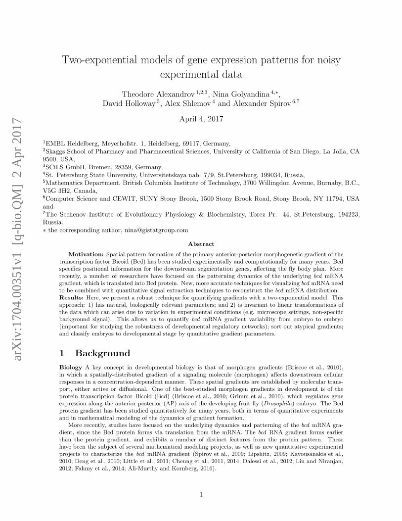
Though the large variability and small sample size do not allow for statistically significant conclusionsfor all comparisons, several observations can be made. In particular, CleavageEarly has the largest averageanterior exponential decay constant of any developmental stage (i.e. the steepest profile). This difference isstatistically significant (t-test), but could be rendered insignificant by moderate changes in just one of thesix embryos. We therefore combine groups to obtain 3 age groups (from 7) with larger sample sizes: (1)Cleavage, n = 19; (2) nc10–nc13, n = 23; (3) nc14, n = 46. Figure 3B shows that these larger groups havemore distinct clustering, with distinct means.

Table 1 shows the average values for λ(apical)anterior and Cab with their 90% confidence intervals.

One-way ANOVA (both parametric and non-parametric (Kruskal-Wallis)) confirms that both λ(apical)anterior

and Cab significantly differ between the groups at the 5% level. Post-hoc comparisons show that Cab (thelogarithm of the ratio between the apical and basal anterior gradients at 10 %EL) is significantly differentbetween all three groups; while the exponential decay rate of the anterior gradient is significantly larger (λis smaller) only for the Cleavage group.

7

A. lambda_ant_apic

Cab

−0.5

0.0

0.5

1.0

1.5

2.0

0.70 0.75 0.80 0.85 0.90 0.95

nc10−12nc13CleavageEarlyCleavageLater

nc14 Early1nc14 Early2nc14 Late

B. lambda_ant_apic

Ca

b

−0.5

0.0

0.5

1.0

1.5

2.0

0.70 0.75 0.80 0.85 0.90 0.95

1 2 3

Figure 3: Pre-exponential factor Cab vs. anterior gradient λ(apical)anterior. A. 7 (marked) developmental stages

(Section 2.2): Two-exponential parameters show large variability between and within the developmental stages.B. 3 combined groups (see key): difference in parameter values, with 90% confidence ellipsoid.

3.3.1 Potentials of the approach

In section 3.2, we screened embryos into Type 1 using condition (A), i.e. non posteriorly-increasing pro-files. We can apply the suggested approach to embryos of Type 2 with posteriorly-increasing profiles (seeFigure 2D). Moreover, the model can be extended to three exponentials (see Figure 4). With the exten-sion of SSA to fit a 3-exponential model, these sorts of patterns can be readily analyzed by the currentapproach, broadening the use of the technique to allow for the comparison of patterns from different genes(e.g., consider Stau protein (Spirov et al., 2009), which has a sharp rise in the vicinity of the posterior pole).

The approach presented here is likely to be an effective tool for quantifying other spatial gradients indevelopmental biology, which could aid in revealing new features in the patterning dynamics and regulationof critical developmental events, especially where there are large dynamic changes and high variability —i.e. in cases where it is difficult to construct a reference or prototype profile. Examples include the Dorsalgradient in DV Drosophila patterning (Kanodia et al., 2012, 2011; Reeves et al., 2012) and retinoic acid invertebrate embryos (Schilling et al., 2012).

Table 1: Combined groups: means and 90% confidence intervals for main characteristics of apical and basalprofiles for 3 groups.

λapicalanterior lower bound upper bound

Cleavage 0.825 0.798 0.853nc10-13 0.880 0.863 0.896nc14 0.872 0.863 0.880

Cab lower bound upper boundCleavage 0.274 0.089 0.459nc10-13 -0.167 -0.296 -0.037nc14 0.657 0.511 0.803

8

AP, %

0

50

100

20 40 60 80

profileESPRIT approxanterior expshallow exptail expresiduals

Figure 4: AP profile of the Stau protein (cf. Spirov et al. (2009, Fig.6)). The raw data is in blue, the 3-exponential model is in red: anterior exponent 1, green; shallow exponent 2, magenta; posterior exponent 3,yellow; residuals, black.

4 Conclusions

The new mathematical model described here enables the study of substantial quantitative problems inbcd mRNA gradient formation, including quantification of the between-embryo variability of the gradient;the filtering of atypical gradients; and the classification of embryos on the basis of quantitative gradientparameters. We are using these abilities to quantitatively study the dynamics of bcd mRNA profiles at veryearly stages of development. Finally, we can also now use the new mRNA gradient model to compare mRNApatterning with the Bcd protein gradient, previously analyzed in Alexandrov et al. (2008).

Acknowledgement

This work has been supported by U.S. NIH grant R01-GM072022 and the Russian Foundation for BasicResearch grants 15-04-06480 and 16-04-00821.

References

T. Alexandrov, N. Golyandina, and A. Spirov. Singular Spectrum Analysis of gene expression profiles ofearly Drosophila embryo: Exponential-in-distance patterns. Res. Lett. in Signal Process., 2008:1–5, 2008.

Z. Ali-Murthy and T. Kornberg. Bicoid gradient formation and function in the Drosophila pre-syncytialblastoderm. eLife, 5:e13222–, 2016.

F. Alonso, J. Castillo, and P. Pintado. Application of singular spectrum analysis to the smoothing of rawkinematic signals. J Biomech, 38(5):1085–1092, 2005.

J. Briscoe, P. A. Lawrence, and J.-P. Vincent, editors. Generation and Interpretation of Morphogen Gradi-

ents: A Subject Collection from Cold Spring Harbor Perspectives in Biology. Cold Spring Harbor, N.Y.:Cold Spring Harbor Laboratory Press, 2010.

S. L. Bullock and D. Ish-Horowicz. Conserved signals and machinery for RNA transport in Drosophilaoogenesis and embryogenesis. Nature, 414(6864):611–616, Dec. 2001.

D. Cheung, C. Miles, M. Kreitman, and J. Ma. Scaling of the Bicoid morphogen gradient by a volume-dependent production rate. Development, 138(13):2741–2749, 2011.

D. Cheung, C. Miles, M. Kreitman, and J. Ma. Adaptation of the length scale and amplitude of theBicoid gradient profile to achieve robust patterning in abnormally large Drosophila melanogaster embryos.Development, 141:124–135], 2014.

9

S. Dalessi, A. Neves, and S. Bergmann. Modeling morphogen gradient formation from arbitrary realisticallyshaped sources. Journal of Theoretical Biology, 294:130 – 138, 2012.

J. Deng, W. Wang, L. J. Lu, and J. Ma. A two-dimensional simulation model of the bicoid gradient inDrosophila. PloS one, 5(4):e10275, 2010.

K. Fahmy, M. Akber, X. Cai, A. Koul, A. Hayder, and S. Baumgartner. αTubulin 67C and Ncd are essentialfor establishing a cortical microtubular network and formation of the Bicoid mRNA gradient in Drosophila.PLoS ONE, 9(11):e112053, 2014.

N. Golyandina. On the choice of parameters in singular spectrum analysis and related subspace-basedmethods. Stat. Interface, 3(3):259–279, 2010.

N. Golyandina and A. Zhigljavsky. Singular Spectrum Analysis for time series. Springer Briefs in Statistics.Springer Berlin Heidelberg, 2013.

N. Golyandina, V. Nekrutkin, and A. Zhigljavsky. Analysis of Time Series Structure: SSA and Related

Techniques. Chapman&Hall/CRC, Boca Raton, 2001.

N. Golyandina, A. Pepelyshev, and A. Steland. New approaches to nonparametric density estimation andselection of smoothing parameters. Comput. Stat. Data Anal., 56(7):2206–2218, 2012.

T. Gregor, W. Bialek, R. de Ruyter van Steveninck, D. Tank, and E. Wieschaus. Diffusion and scalingduring early embryonic pattern formation. Proc. Nat. Acad. Sci. USA, 102:18403–18407, 2005.

T. Gregor, D. Tank, E. Wieschaus, and W. Bialek. Probing the limits of positional information. Cell, 130:153–164, 2007.

T. Gregor, A. McGregor, and E. Wieschaus. Shape and function of the bicoid morphogen gradient in dipteranspecies with different sized embryos. Dev. Biol., 316:350–358, 2008.

O. Grimm, M. Coppey, and E. Wieschaus. Modelling the Bicoid gradient. Development, 137, 2010.

D. Holloway, L. Harrison, D. Kosman, C. Vanario-Alonso, and A. Spirov. Analysis of pattern precisionshows that Drosophila segmentation develops substantial independence from gradients of maternal geneproducts. Dev. Dyn., 235:2949–2960, 2006.

B. Houchmandzadeh, E. Wieschaus, and S. Leibler. Establishment of developmental precision and propor-tions in the early Drosophila embryo. Nature, 415:798–802, 2002.

J. Kanodia, H.-L. Liang, Y. Kim, B. Lim, M. Zhan, H. Lu, C. Rushlow, and S. Shvartsman. Patternformation by graded and uniform signals in the early Drosophila embryo. Biophysical Journal, 102(3):427–433, 2012.

J. S. Kanodia, Y. Kim, R. Tomer, Z. Khan, K. Chung, J. D. Storey, H. Lu, P. J. Keller, and S. Y. Shvartsman.A computational statistics approach for estimating the spatial range of morphogen gradients. Development,138(22):4867–4874, 2011.

M. E. Kavousanakis, J. S. Kanodia, Y. Kim, I. G. Kevrekidis, and S. Y. Shvartsman. A compartmentalmodel for the bicoid gradient. Developmental Biology, 345(1):12 – 17, 2010.

H. D. Lipshitz. Follow the mRNA: a new model for Bicoid gradient formation. Nat Rev Mol Cell Biol, 10(8):509–512, Aug. 2009. ISSN 1471-0072. URL http://dx.doi.org/10.1038/nrm2730.

S. Little, G. Tkacik, T. Kneeland, E. Wieschaus, and T. Gregor. The formation of the Bicoid morphogengradient requires protein movement from anteriorily localized mRNA. PLoS Biology, 9(e1000596), 2011.

W. Liu and M. Niranjan. Gaussian process modelling for bicoid mRNA regulation in spatio-temporal Bicoidprofile. Bioinformatics, 28(3):366–372, 2012.

E. Myasnikova, M. Samsonova, D. Kosman, and J. Reinitz. Removal of background signal from in situ dataon the expression of segmentation genes in Drosophila. Development Genes and Evolution, 215:320–326,2005.

G. T. Reeves, N. Trisnadi, T. V. Truong, M. Nahmad, S. Katz, and A. Stathopoulos. Dorsal-ventral geneexpression in the Drosophila embryo reflects the dynamics and precision of the dorsal nuclear gradient.Developmental cell, 22(3):544–557, Feb. 2012.

10

R. Roy and T. Kailath. ESPRIT: estimation of signal parameters via rotational invariance techniques. IEEETrans. Acoust., 37:984–995, 1989.

T. F. Schilling, Q. Nie, and A. D. Lander. Dynamics and precision in retinoic acid morphogen gradients.Current opinion in genetics & development, 22(6):562–569, Dec. 2012.

A. Shlemov, N. Golyandina, D. Holloway, and A. Spirov. Shaped 3D singular spec-trum analysis for quantifying gene expression, with application to the early Drosophila

embryo. BioMed Research International, 2015(Article ID 986436):1–18, 2015a. URLhttp://downloads.hindawi.com/journals/bmri/raa/986436.pdf .

A. Shlemov, N. Golyandina, D. Holloway, and A. Spirov. Shaped singular spectrum analysis for quantifyinggene expression, with application to the early Drosophila embryo. BioMed Research International, 2015(Article ID 689745), 2015b. URL http://downloads.hindawi.com/journals/bmri/raa/689745.pdf.

A. Spirov, K. Fahmy, M. Schneider, E. Frei, M. Noll, and S. Baumgartner. Formation of the bicoid morphogengradient: an mRNA gradient dictates the protein gradient. Development, 136:605–614, 2009.

A. V. Spirov, N. E. Golyandina, D. M. Holloway, T. Alexandrov, E. N. Spirova, and F. J. P. Lopes. Mea-suring gene expression noise in early Drosophila embryos: the highly dynamic compartmentalized micro-environment of the blastoderm is one of the main sources of noise. Springer Verlag Lecture Notes in

Computer Science, 7246:177–188, 2012.

S. Surkova, D. Kosman, K. Kozlov, Manu, E. Myasnikova, A. A. Samsonova, A. Spirov, C. E. Vanario-Alonso,M. Samsonova, and J. Reinitz. Characterization of the Drosophila segment determination morphome.Developmental Biology, 313(2):844–862, 2008.

T. T. Weil, K. M. Forrest, and E. R. Gavis. Localization of bicoid mRNA in late oocytes is maintained bycontinual active transport. Developmental Cell, 11(2):251–262, 2006. ISSN 1534-5807.

T. T. Weil, R. Parton, I. Davis, and E. R. Gavis. Changes in bicoid mRNA anchoring highlight conservedmechanisms during the oocyte-to-embryo transition. Current biology : CB, 18(14):1055–1061, July 2008.

11

Supplementary materials

A Data

A.1 FISH and data acquisition

Images (1024 × 1024 pixels, 8 bit) were taken using confocal microscopy Spirov et al. (2009). Images wereacquired through whole embryo stacks, and suitable mid-sagittal slices were selected to eliminate unnecessarygeometric distortion. Using the raw data directly from the confocal microscope, intensities were measuredby sliding an area perpendicular to the embryo edge, similar to Houchmandzadeh et al. (2002), but with ourown algorithms, scripts and tools (below). One curve followed the dorsal apical periplasm, while the othercurve followed the dorsal basal periplasm.

A.2 Computational Tools to Process Images

Our tools consisted of a set of plug-ins for ImageJ software (W. Rasband, NIH, USA) and scripts in Delphi(for Windows) or GnuPascal (for Linux). After raw image rotation and cropping, the software is used tofind the image contour (dorsal or ventral edge of embryo). This contour is used to find a series of curvilinearprofiles (lines) running beneath and in parallel to the contour. The two main (apical and basal) profileswere chosen by visual inspection. Local intensity data was collected along these profiles. A small circularwindow of a given radius R (in pixels), or Region Of Interest (ROI), is centered on the profile. The ROI isslid in steps of one pixel along the profile. At each step, the intensity is measured and averaged over theROI and saved. This method of measuring overlapping areas of averaged intensities served as a first stepin de-noising the (noisy) FISH images. (A second step of de-noising was done with SSA, see below). Forapical profiles, a radius of 3 pixels was used for the ROI, covering a thin layer of apical periplasm betweenthe nuclear membrane and plasma membrane along the dorsal axis. For the basal periplasm, two radii, R= 5 and R = 12 pixels, were tested (the basal periplasm is substantially wider than the apical periplasm).R = 5 is sufficient to collect the representative data. To the best of our knowledge, all prior work on suchDrosophila data has involved a projection of the natural (ellipsoidal) surface curvilinear coordinates to theAP axis (running down the center of the embryo; (Gregor et al. (2005, 2007, 2008); Houchmandzadeh et al.(2002); Little et al. (2011); Cheung et al. (2011, 2014)). The distortion of patterns at the very tip of anembryo for such a projection could be substantial. Therefore, we tested the present results on both thenatural curvilinear coordinates and on the AP projection.

B Mathematical details of ESPRIT

Here, we describe the ESPRITmethod (specifically LS-ESPRITRoy and Kailath (1989),(Golyandina and Zhigljavsky,2013, Section 3.8.2)) applied to a sequence of observations x1, x2, . . . , xN , where

xn = sn + εn, sn = C1 exp(α1n) + C2 exp(α2n), (6)

εn is a noise.Fix the signal rank r (number of exponentials in our case) and choose a window length r+1 ≤ L ≤ N−r.

We chose L ≈ N/2 to get better separability of the signal from noise, see Golyandina (2010), and haver = 2. The first step consists in the construction of the trajectory matrix X from the column vectorsXi = (xi, . . . , xi+L−1)

T, i = 1, . . . ,K = N − L+ 1: X = [X1 : · · · : XL]. ESPRIT is based on the SingularValue Decomposition (SVD) of the matrix X. Let U = [U1 : · · · : Ur] be the matrix consisting of the rleading left singular vectors of X. Denote by U the matrix U without the last row and by U the matrixU without the first row. Consider the (r × r)-matrix Λ = U−U, where A− stands for pseudo-inverse of

A. The eigenvalues of Λ provide the ESPRIT-estimates λi of λ1 and λ2, where λi = exp(αi), see (6).Coefficients Ci in (6) can be found by means of the ordinary least-squares method in the linear model

xn = C1z(1)n + C2z

(2)n + εn, where z

(i)n = λn

i .

12

C Data processing

C.1 Filtering of embryos

Figure 5 shows scatterplots of λ(apical)anterior, λ

(basal)anterior, λ

(apical)shallow and λ

(basal)shallow before and after application of the

constraints. Most outlier embryos were filtered out, making the distribution of profile parameters morehomogeneous.

We consider embryos with non-increasing shallow exponential: (A) λ(apical)shallow < 1.002, λ

(basal)shallow < 1.002.

The outliers can be found by standard tools basing on 2D scatterplots of the estimated parameters. Itappears that the outliers can be removed by the conditions data (B) AP0

(apical)anterior ≤ 120, AP0

(basal)anterior ≤ 120

and (C) Cab > −1.Table 2 shows the proportion of embryos, by stage, satisfying conditions (A), (B), and (C). The number

of embryos excluded is highest for Cleavage stage; exclusion here is chiefly by criterion (A), reflecting thatearly stage embryos are more likely to have posteriorly-increasing shallow gradients than later stage embryos(33% for Cleavage; 17% for nc10-13; 7% for nc14. (For embryos not excluded by criteria (B) and (C), theproportion of the embryos with posteriorly-increasing shallow gradient was: 17% Cleavage; 8% nc10-13; 0%nc14.)

Table 2: Proportion of embryos satisfying criteria (A), (B) and (C) individually and combined, from the wholedataset of embryos.

group N (A) (B) (C) (A),(B),(C)Cleavage 19 66% 76% 79% 50%10-13 cycle 23 83% 90% 90% 77%14 cycle 46 93% 88% 91% 82%

88 embryos satisfy conditions (A)–(C), from the complete dataset of 124 embryos (Table 2); the analysisin the rest of this paper is on these 88 embryos.

13

A

lambda_ant_apic

0.75 0.85 0.95 1.00 1.04

0.6

50

.90

0.7

50

.95

lambda_ant_bas

lambda_sh_apic

0.9

85

1.0

10

0.65 0.80 0.95

1.0

01

.06

0.985 1.000 1.015

lambda_sh_bas

Before

B

lambda_ant_apic

0.75 0.85 0.990 0.996

0.7

00

.90

0.7

50

.90

lambda_ant_bas

lambda_sh_apic

0.9

90

1.0

00

0.70 0.80 0.90

0.9

90

1.0

00

0.990 0.996

lambda_sh_bas

After

Figure 5: Scatterplots of λ(apical)anterior, λ

(basal)anterior, λ

(apical)shallow , and λ

(basal)shallow, before (A) and after (B) application of the

constraints.

14

C.2 The model accuracy

Systematic error. Here, we analyze the adequacy of the two-exponential model using an examplefrom the Early2 sub-stage of nc14; these results are typical of the two-exponential fit. It can be seen inFigure 6A (black) that the noise is not homogeneous (it has changing variability); the averaged residuals(red line; Figure 6A) show this systematic error as a function of the AP coordinate. However, this variationis of magnitude no more than two intensity units (greatest near the inflection point, at the switch betweenthe two exponential components), which is negligible relative to the residual noise or to the profile itselfFigure 6B.

A

20 40 60 80

−30

−10

10

30

AP B AP, %

0

50

100

20 40 60 80

profileESPRIT approxanterior expshallow expresiduals

Figure 6: Noise and trend for a cycle 14 embryo. A. Residuals, showing a systematic variation. B. Model fittingto data (above) and residuals (below).

Table 3 shows the root mean square error (RMSE) of residuals across developmental stages. These arealways significantly smaller than the magnitude of the profile intensities. Table 3 shows that the system-atic error, computed by applying a median filter of 40%EL, never exceeds 1.0, negligible on the profileintensity range. (Note that both the RMSE of residuals and of systematic error components decrease withdevelopmental age; earlier profiles show stronger noise. However, this effect is not independent of a lineartransformation of profiles and therefore can be caused by different microscope settings.) Overall, the modelclosely approximates the data profiles, leaving chiefly non-systematic noise in the residuals.

C.3 Comparison with ‘exponential plus constant’ model

Table 3: Characteristics of residuals after fitting the ‘exponential plus constant’ and the two-exponential modelsto the mRNA profiles.

exp+const 2-expresidual RMSE residual RMSE systematic RMSEapical basal apical basal apical basal

Cleavage 5.5 5.0 4.7 4.7 1.0 1.0nc10–13 4.7 4.7 4.2 3.0 0.8 0.7nc14 5.5 2.6 4.1 2.0 0.6 0.4

Single-exponential-plus-constant-background models have been used in a number of studies of /Bcdprofiles, both protein Houchmandzadeh et al. (2002) and mRNA Spirov et al. (2009). Table 3 demonstratesthat the two-exponential model fits the mRNA profiles better (MSE is smaller) than such exponential-plus-constant models. These results are not too surprising, since the two-exponential model is not constrainedto have a flat background.

C.4 Curvilinear coordinates

Here, we test that the results of fitting the two-exponential model is robust to small non-linear transforma-tions. That is, we test for differences in using AP projections (ignoring the DV coordinate) vs. curvilinearcoordinates along the profile in the image (d2(i) = (AP(i+1)−AP(i))2 +(DV(i+1)−DV(i))2; cumulativedistances are then normalized by dividing by the sum of d(i)): see Figure 7.

15

A

0 20 40 60 80 100

10

30

50

70

AP

DV

B AP, %

0

50

100

20 40 60 80

profileESPRIT approxanterior expshallow expresiduals

C AP, %

0

50

100

20 40 60 80

profileESPRIT approxanterior expshallow expresiduals

Figure 7: 1D profiles: curvilinear coordinates vs. AP projections. A. original AP, DV coordinates of thesampled nuclei. B. 1D intensity profile and ESPRIT analysis on an AP projection (DV coordinate not used).C. 1D intensity profile and ESPRIT analysis using curvilinear coordinates.

Table 4 shows the mean values of the model characteristics for both AP and curvilinear coordinates(MSE: mean squared data-to-model difference). MSE is smaller for AP than curvilinear for all groups

except CleavageEarly. Values of λ(apical)anterior are larger with curvilinear coordinates, but this stems from the

way the coordinates are constructed – distances between points in curvilinear coordinates near the profileedges are larger than that for direct AP coordinates. The results in Table 4 indicates that conclusions foundusing AP coordinates are valid with respect to curvilinear coordinates, and that the two-exponential modelis robust to moderate deviations in the data.

16

Table 4: Mean characteristics for AP and curvilinear coordinatesAP-coordinates λ

(apical)anterior MSE,

apicalλ(basal)anterior MSE,

basalCab

CleavageEarly 0.79 15.77 0.78 13.86 0.11CleavageLater 0.84 25.93 0.86 29.32 0.35nc10–12 0.88 19.17 0.86 14.35 -0.21nc13 0.88 17.94 0.85 5.63 -0.21nc14 early1 0.88 17.52 0.83 4.56 0.40nc14 early2 0.86 17.95 0.85 3.81 0.99nc14 late 0.87 10.40 0.86 1.93 1.33

Curvilinear coordinates λ(apical)anterior MSE,

apicalλ(basal)anterior MSE,

basalCab

CleavageEarly 0.84 12.63 0.81 13.73 0.01CleavageLater 0.85 26.83 0.88 30.89 0.24nc10–12 0.91 20.63 0.90 16.48 -0.14nc13 0.91 20.53 0.89 6.73 -0.23nc14 early1 0.91 19.11 0.87 4.99 0.49nc14 early2 0.90 20.10 0.89 4.10 1.12nc14 late 0.90 11.23 0.92 2.13 1.59

17