Journal of Hydrology 399 (2011) 246–254

Contents lists available at ScienceDirect

Journal of Hydrology

journal homepage: www.elsevier .com/locate / jhydrol

Experimental study of solute transport under non-Darcian flow in a single fracture

Jiazhong Qian a,1, Hongbin Zhan b,c,⇑, Zhou Chen a,1, Hao Ye a,1

a School of Resources and Environmental Engineering, Hefei University of Technology, Hefei 230009, Chinab Department of Geology & Geophysics, Texas A&M University, College Station, TX 77843-3115, USAc Faculty of Engineering and School of Environmental Studies, China University of Geosciences, Wuhan, Hubei 430074, China

a r t i c l e i n f o s u m m a r y

Article history:Received 7 January 2010Received in revised form 4 January 2011Accepted 6 January 2011Available online 12 January 2011

This manuscript was handled by P. Baveye,Editor-in-Chief

Keywords:Boundary layer dispersionNon-Fickian transportTracer testSimulationAnalytical solution

0022-1694/$ - see front matter � 2011 Elsevier B.V. Adoi:10.1016/j.jhydrol.2011.01.003

⇑ Corresponding author at: Department of GeologUniversity, College Station, TX 77843-3115, USA. Tel.:845 6162.

E-mail addresses: qjiazhong@gmail.com (J. Qian), z(H. Zhan).

1 Tel.: +86 0551 2901524; fax: +86 0551 2904517.

We have experimentally studied solute transport in a single fracture (SF) under non-Darcian flow condi-tion which was found to closely follow the Forchheimer equation at Reynolds numbers around 12.2–86.0when fracture apertures were between 4 mm and 9 mm. The measured breakthrough curves (BTCs)under the non-Darcian flow condition had some features that are difficult to explain using the Fickiantype advection–dispersion equation (ADE). All the measured BTCs showed long tails, which might becaused by mass transfer between the boundary layer near the fracture wall and the mobile domain nearthe plane of symmetry, as supported by the boundary layer dispersion theories of Koch and Brady (1985,1987). A mobile–immobile (MIM) model was used to simulate the measured BTCs. To show that the MIMmodel was doing a better job than the ADE model in describing the observed BTCs, we conducted statis-tical analysis on the goodness of fitting with these two models. The results showed that the correlationcoefficients for the MIM model were greater than those for the ADE model and were close to unity, indi-cating a nearly perfect fit with the MIM. The mass transfer rate between the mobile domain and theboundary layer increased when the mobile water fraction became larger. The best fit dispersivity valuesusing the MIM model varied between 1.05 mm and 9.29 mm whereas their counterparts using the ADEmodel varied between 245 mm and 462 mm for the experimental condition of this study. Several issuessuch as the possible bimodal concentration distribution and the scale-dependent transport in a SF werediscussed and would be investigated in the future.

� 2011 Elsevier B.V. All rights reserved.

1. Introduction

For many decades, the Fick’s law was believed to be the govern-ing law of transport in the subsurface where the dispersive massflux was assumed to be proportional to the first derivative of thesolute concentration (Bear, 1972; Fetter, 1999). The governingequation derived based on the Fick’s law was the well-knownadvection–dispersion equation (ADE) (Bear, 1972). If the Fickiantransport model works, it will predict a well behaved breakthroughcurve (BTC), which can be described by a Gaussian distributionfunction in a homogeneous aquifer for one-dimensional transportwith a pulse source (Bear, 1972; Fetter, 1999). However, extensiveevidence had shown different findings. In summary, there weretwo striking features that cannot be explained by the Fickian trans-port model. First, peak value of BTC arrived earlier than what wasexpected from ADE (early arrival); second, tailing of the BTC lasted

ll rights reserved.

y & Geophysics, Texas A&M+1 979 862 7961; fax: +1 979

han@geosmail.tamu.edu

much longer than what was predicted from ADE (long tail); third,concentration profile was sometime observed to be bimodal.

Non-Fickian transport phenomena were observed in a singlefracture (SF) (Dronfield and Silliman, 1993; Masciopinto, 1999;Detwiler et al., 1999; Bodin et al., 2003; Brush and Thomson,2003; Boutt et al., 2006; Bauget and Fourar, 2008; Cardenaset al., 2007; Cardenas, 2008) and in a fractured medium(Hadermann and Heer, 1996; Sidle et al., 1998; Becker and Shapiro,2000; McKay et al., 2000; Kosakowski et al., 2001) for a long time.There were several attempts of searching for explanation on non-Fickian transport. This included the continuous time random walk(CTRW) (Scher and Lax, 1973; Kosakowski et al., 2001); thefractional advection–dispersion equation (FADE) (Benson, 1998;Baeumer et al., 2005); the mobile–immobile approach (MIM)(Coats and Smith, 1964; Piquemal, 1992, 1993); and the boundarylayer dispersion (Koch and Brady, 1985, 1987; Moutsopoulos andKoch, 1999), among others.

Up to now, most non-Fickian transport models in subsurfacehydrology were based on the Darcian flow scheme which assumeda linear relationship between the specific discharge and thehydraulic gradient. Non-Darcian flow can arise from a number ofdifferent ways in porous and fractured media. For instance,increasing inertial force along with the increase of flow speed

J. Qian et al. / Journal of Hydrology 399 (2011) 246–254 247

and onset of turbulent flow can lead to non-Darcian flow. Non-Dar-cian flow is particularly easy to occur in a SF (e.g. Lomize, 1951;Louis, 1969; Maini, 1971; Sharp and Maini, 1972; Iwai, 1976; Qianet al., 2005, 2007, 2010; Wen et al., 2006) due to relatively highflow velocities there. Qian et al. (2005) summarized someevidences of non-Darcian flow in a SF. Recent studies of Wenet al. (2006) and Moutsopoulos (2009) dealt with analytical andsemi-analytical solutions of transient non-Darcian flow. Javadiet al. (2010) investigated the subject of determining the flow resis-tance coefficient and put forward a new geometrical model fornon-linear fluid flow through rough fractures.

How is the transport process under the non-Darcian flow dif-ferent from that under the Darcian flow in a SF? What is the ade-quate conceptual model to describe solute transport in a SF underthe non-Darcian flow condition? These are the questions we tryto answer in this study. The reason for choosing a SF to studyis because of its relevance in many disciplines such as hydrology,tectonics, petroleum engineering with various applicationsincluding nuclear waste repository. For flow in a SF, a region oflow velocities occurs near the solid boundary (fracture wall)due to the no-slip condition and a region of high velocities occursnear the plane of symmetry. The influence of the velocity contrastin these two regions on the dispersion process was investigatedby Koch and Brady (1985) for a dilute porous medium (a porousmedium having a porosity near unity), and by Moutsopoulos andKoch (1999) for a non-dilute, homogeneous and heterogeneousporous medium. This dispersion mechanism was called boundarylayer dispersion by Koch and Brady (1985) and Moutsopoulos andKoch (1999). Koch and Brady (1987) studied the non-Fickianboundary layer dispersion problem based on a nonlocal disper-sion theory.

Some other recent studies on solute transport in a SF had beensummarized by Qian et al. (2011) who also performed experimen-tal study of flow and solute transport in a sand-filled SF and dem-onstrated that the mobile–immobile (MIM) model was reasonablefor explaining the long tailing of the observed BTCs. Another re-lated recent study was reported by Bauget and Fourar (2008)who investigated non-Fickian transport in a rough walled SF. Threedifferent models including ADE, CTRW, and a stratified model wereemployed by Bauget and Fourar (2008) to interpret the tracerexperiments. Bauget and Fourar (2008) designed an impressive im-age processing method to obtain realistic information of fractureaperture and solute concentration distributions in the SF. The mod-eling work of Bauget and Fourar (2008), however, had two pointsthat were debatable, as far as we understood the problem. The firstpoint was related to the averaging procedure along the width ofthe fracture (the y-axis) to obtain averaged BTCs (see Bauget andFourar, 2008, p. 143). Given the heterogeneous nature of the aper-ture distribution, one was not surprising to see that flow and trans-port in such a SF was channeled with several preferentialpathways, as can be seen from Fig. 6 of Bauget and Fourar(2008). A great deal of important information regarding such chan-neled transport was lost after averaging concentration along the y-axis. A better way of interpreting the transport data must considerthe nature of channeled transport. The second point was associatedwith the stratified model used by Bauget and Fourar (2008). In thismodel, the hydraulic conductivity distribution was assumed to benormal (Gaussian) by Bauget and Fourar (2008). Although the nor-mal distribution of hydraulic conductivity was not necessarilyincorrect, the most commonly used hydraulic conductivity distri-bution in the literature was log-normal (Fetter, 1999). In fact, Zhan(1998) provided some closed-form analytical solutions and analy-sis of solute transport in a stratified aquifer considering the log-normal distribution of hydraulic conductivity. The solutions ofZhan (1998) may be applicable for reinterpreting the data ofBauget and Fourar (2008).

Our overarching objective is conducting a series of controlledlaboratory experiments to investigate solute transport under thenon-Darcian flow condition in a SF. Qian et al. (2011) was onephase of research that dealt with a sand-filled SF. This study wasanother phase of research that dealt with an open SF. It is desirableto use a real SF to carry out the experiments. However, the geomet-ric complexity of a real SF may cause some problems for interpret-ing the data. To avoid any unnecessary ambiguity, we used aparallel-plane SF in the experiments. Although the parallel-planeSF is a highly idealized one, this knowledge will provide a goodbenchmark case to compare with further investigation of solutetransport in a real (rough) SF under the non-Darcian flow. Qianet al. (2011) further elaborated the rationale of using an idealizedSF for the experiments.

2. Experimental methods

2.1. Experimental setup

The experimental setup was very similar to that of Qian et al.(2011), thus was only briefly illustrated here. The physical modelemployed was built of Plexiglass plates which allowed both visualand electronic monitoring of tracer movement by using dye andtracer added to the solutions. Each fracture plane was 1000 mmin length, 10 mm in width and 250 mm in height. The SF was ver-tical and opened at the top. A tracer injection device was located100 mm downstream from the recharge flume on the left. In addi-tion, a water sample collection device was located 95 mm up-stream from the discharge flume on the right. So the distancefrom the tracer injection position to the sample collection positionwas 805 mm (subtracting 100 mm and 95 mm from 1000 mmwhich was the length of the SF).

2.2. Experimental methods

First, a series of flow experiments were performed in SFs withdifferent apertures (9 mm, 7 mm, 6 mm, and 4 mm) and differenthydraulic gradients (0.0005–0.0084). To determine the relation-ship between the average velocity and the hydraulic gradient, sev-eral water level differences between the recharge and dischargeflumes were chosen and the corresponding flow rates were re-corded. The associated Reynolds numbers (Re) were calculated by

Re ¼Vbm; ð1Þ

where V was the average flow velocity in the fracture; b was theaverage aperture and m was the kinematic viscosity. The values ofm at 15 �C and 20 �C are 1.140 mm2/s and 1.005 mm2/s, respectively(Munson et al., 1998, Table B.2). A point to note was that the aper-ture b was chosen as the characteristic length of flow in above Eq.(1). Other studies may choose a different characteristic length suchas the length of the SF to define the Re. Be aware that the Re calcu-lated with the length of the SF as the characteristic length can beconsiderably greater than what is calculated from Eq. (1).

Plots of the average velocity versus the hydraulic gradient willtest whether Darcy’s law was valid or not. Steady-state flow rateswere monitored using a calibrated flow meter LZB-25 (glass Rota-meter made in Shanghai, China) with errors less than 1.5%. Thewater levels were measured with piezometers distributed uni-formly along the flow path in the fracture, with errors less than0.5 mm. Each measurement was repeated three times and theaverage value was used for further calculation.

To study solute transport in a SF, tracer tests were carried outusing a conservative tracer sodium chloride (NaCl). A pilot dye tra-cer experiment was carried out to determine the first and last

248 J. Qian et al. / Journal of Hydrology 399 (2011) 246–254

arrival times before the NaCl tracer tests. These times were used asreferences of choosing sample collection times. After the pilot test,solution of NaCl with a volume of 5 mL and a concentration of1000 mg/L was well-mixed and injected instantaneously from thetracer injection device. The tracer injection device and the watersample collection device were vertical pipes with extremely smalldiameters (around 1 mm) to minimize the disturbance to the flowfield. In order to minimize the disturbance of the injected solute tothe flow, the 5 mL NaCl solute was evenly injected through manysmall slots over the vertical injecting pipe. Preliminary injectiontest with the red dye (not shown here) indicated that disturbanceto the flow field by the injecting method was not apparent. Afterthat, water samples each with a volume of 2.5 mL were collectedfrom the sample collection device, started 20 s before the first arri-val time and ended 40 s after the last arrival time. The volume ofthe collected water samples during each experiment was small en-ough not to affect the flow through the SF. This can be easily illus-trated. For instance, for a representative flow rate of 5.43 mL/s anda representative duration of flow about 200 s, the total volume offlow was about 1086 mL. Assuming 20 samples each with a volumeof 2.5 mL were taken, the total volume of the samples was 50 mL,which was only about 4.6% of the total flow volume, thus was re-garded as negligible.

The values of conductance ls of the water samples were mea-sured by a conductance instrument DDS-307 (Shanghai Automa-tion Instrumentation Co., Shanghai, China) with errors less than0.1%. Based on the concentration of the injected NaCl and the mea-sured electric conductance, a regressive equation was established:

C ¼ 0:683ls; ð2Þ

where C was the concentration of NaCl solution (mg/L) and ls wasthe measured electric conductance (in microsiemens). The correla-tion coefficient of Eq. (2) was very close to unity (0.999), indicatinga nearly perfect linear relationship between C and ls. Thus, C can beprecisely calculated by measuring ls via Eq. (2).

To find out if flow was Darcian or non-Darcian, flow experi-ments were repeated three times to ensure the accuracy. After that,one tracer test was carried out for each of four different flow veloc-ities for a SF with a 4 mm aperture. The temperature during theexperiment was between 15 �C and 20 �C.

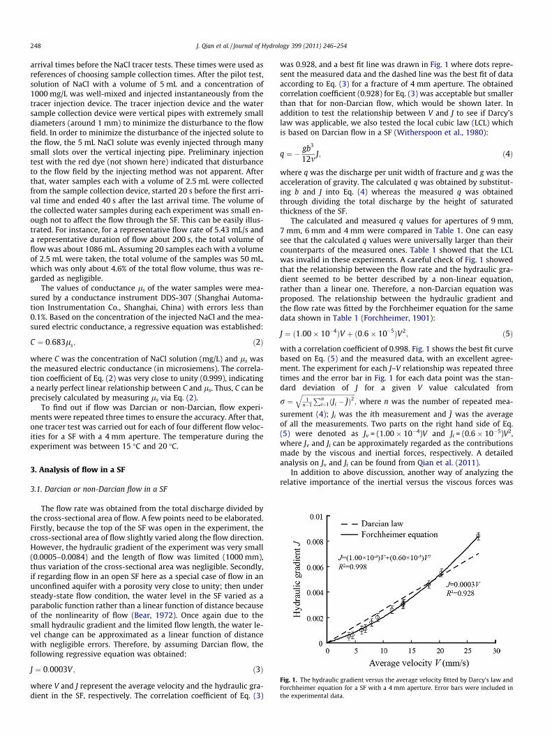
ig. 1. The hydraulic gradient versus the average velocity fitted by Darcy’s law andorchheimer equation for a SF with a 4 mm aperture. Error bars were included ine experimental data.

3. Analysis of flow in a SF

3.1. Darcian or non-Darcian flow in a SF

The flow rate was obtained from the total discharge divided bythe cross-sectional area of flow. A few points need to be elaborated.Firstly, because the top of the SF was open in the experiment, thecross-sectional area of flow slightly varied along the flow direction.However, the hydraulic gradient of the experiment was very small(0.0005–0.0084) and the length of flow was limited (1000 mm),thus variation of the cross-sectional area was negligible. Secondly,if regarding flow in an open SF here as a special case of flow in anunconfined aquifer with a porosity very close to unity; then understeady-state flow condition, the water level in the SF varied as aparabolic function rather than a linear function of distance becauseof the nonlinearity of flow (Bear, 1972). Once again due to thesmall hydraulic gradient and the limited flow length, the water le-vel change can be approximated as a linear function of distancewith negligible errors. Therefore, by assuming Darcian flow, thefollowing regressive equation was obtained:

J ¼ 0:0003V ; ð3Þ

where V and J represent the average velocity and the hydraulic gra-dient in the SF, respectively. The correlation coefficient of Eq. (3)

was 0.928, and a best fit line was drawn in Fig. 1 where dots repre-sent the measured data and the dashed line was the best fit of dataaccording to Eq. (3) for a fracture of 4 mm aperture. The obtainedcorrelation coefficient (0.928) for Eq. (3) was acceptable but smallerthan that for non-Darcian flow, which would be shown later. Inaddition to test the relationship between V and J to see if Darcy’slaw was applicable, we also tested the local cubic law (LCL) whichis based on Darcian flow in a SF (Witherspoon et al., 1980):

q ¼ � gb3

12mJ; ð4Þ

where q was the discharge per unit width of fracture and g was theacceleration of gravity. The calculated q was obtained by substitut-ing b and J into Eq. (4) whereas the measured q was obtainedthrough dividing the total discharge by the height of saturatedthickness of the SF.

The calculated and measured q values for apertures of 9 mm,7 mm, 6 mm and 4 mm were compared in Table 1. One can easysee that the calculated q values were universally larger than theircounterparts of the measured ones. Table 1 showed that the LCLwas invalid in these experiments. A careful check of Fig. 1 showedthat the relationship between the flow rate and the hydraulic gra-dient seemed to be better described by a non-linear equation,rather than a linear one. Therefore, a non-Darcian equation wasproposed. The relationship between the hydraulic gradient andthe flow rate was fitted by the Forchheimer equation for the samedata shown in Table 1 (Forchheimer, 1901):

J ¼ ð1:00� 10�4ÞV þ ð0:6� 10�5ÞV2; ð5Þ

with a correlation coefficient of 0.998. Fig. 1 shows the best fit curvebased on Eq. (5) and the measured data, with an excellent agree-ment. The experiment for each J–V relationship was repeated threetimes and the error bar in Fig. 1 for each data point was the stan-dard deviation of J for a given V value calculated from

r ¼ffiffiffiffiffiffiffiffiffiffiffiffiffiffiffiffiffiffiffiffiffiffiffiffiffiffiffiffiffiffiffiffiffiffi

1n�1

Pni¼1ðJi ��JÞ2

q; where n was the number of repeated mea-

surement (4); Ji was the ith measurement and �J was the averageof all the measurements. Two parts on the right hand side of Eq.(5) were denoted as Jv = (1.00 � 10�4)V and Ji = (0.6 � 10�5)V2,where Jv and Ji can be approximately regarded as the contributionsmade by the viscous and inertial forces, respectively. A detailedanalysis on Jv and Ji can be found from Qian et al. (2011).

In addition to above discussion, another way of analyzing therelative importance of the inertial versus the viscous forces was

FFth

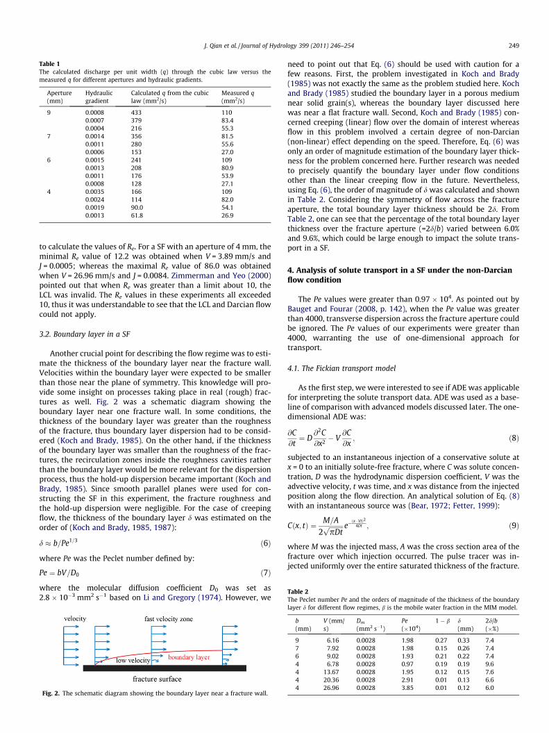
Table 1The calculated discharge per unit width (q) through the cubic law versus themeasured q for different apertures and hydraulic gradients.

Aperture(mm)

Hydraulicgradient

Calculated q from the cubiclaw (mm2/s)

Measured q(mm2/s)

9 0.0008 433 1100.0007 379 83.40.0004 216 55.3

7 0.0014 356 81.50.0011 280 55.60.0006 153 27.0

6 0.0015 241 1090.0013 208 80.90.0011 176 53.90.0008 128 27.1

4 0.0035 166 1090.0024 114 82.00.0019 90.0 54.10.0013 61.8 26.9

Table 2The Peclet number Pe and the orders of magnitude of the thickness of the boundary

J. Qian et al. / Journal of Hydrology 399 (2011) 246–254 249

to calculate the values of Re. For a SF with an aperture of 4 mm, theminimal Re value of 12.2 was obtained when V = 3.89 mm/s andJ = 0.0005; whereas the maximal Re value of 86.0 was obtainedwhen V = 26.96 mm/s and J = 0.0084. Zimmerman and Yeo (2000)pointed out that when Re was greater than a limit about 10, theLCL was invalid. The Re values in these experiments all exceeded10, thus it was understandable to see that the LCL and Darcian flowcould not apply.

3.2. Boundary layer in a SF

Another crucial point for describing the flow regime was to esti-mate the thickness of the boundary layer near the fracture wall.Velocities within the boundary layer were expected to be smallerthan those near the plane of symmetry. This knowledge will pro-vide some insight on processes taking place in real (rough) frac-tures as well. Fig. 2 was a schematic diagram showing theboundary layer near one fracture wall. In some conditions, thethickness of the boundary layer was greater than the roughnessof the fracture, thus boundary layer dispersion had to be consid-ered (Koch and Brady, 1985). On the other hand, if the thicknessof the boundary layer was smaller than the roughness of the frac-tures, the recirculation zones inside the roughness cavities ratherthan the boundary layer would be more relevant for the dispersionprocess, thus the hold-up dispersion became important (Koch andBrady, 1985). Since smooth parallel planes were used for con-structing the SF in this experiment, the fracture roughness andthe hold-up dispersion were negligible. For the case of creepingflow, the thickness of the boundary layer d was estimated on theorder of (Koch and Brady, 1985, 1987):

d � b=Pe1=3 ð6Þ

where Pe was the Peclet number defined by:

Pe ¼ bV=D0 ð7Þ

where the molecular diffusion coefficient D0 was set as2.8 � 10�3 mm2 s�1 based on Li and Gregory (1974). However, we

Fig. 2. The schematic diagram showing the boundary layer near a fracture wall.

need to point out that Eq. (6) should be used with caution for afew reasons. First, the problem investigated in Koch and Brady(1985) was not exactly the same as the problem studied here. Kochand Brady (1985) studied the boundary layer in a porous mediumnear solid grain(s), whereas the boundary layer discussed herewas near a flat fracture wall. Second, Koch and Brady (1985) con-cerned creeping (linear) flow over the domain of interest whereasflow in this problem involved a certain degree of non-Darcian(non-linear) effect depending on the speed. Therefore, Eq. (6) wasonly an order of magnitude estimation of the boundary layer thick-ness for the problem concerned here. Further research was neededto precisely quantify the boundary layer under flow conditionsother than the linear creeping flow in the future. Nevertheless,using Eq. (6), the order of magnitude of d was calculated and shownin Table 2. Considering the symmetry of flow across the fractureaperture, the total boundary layer thickness should be 2d. FromTable 2, one can see that the percentage of the total boundary layerthickness over the fracture aperture (=2d/b) varied between 6.0%and 9.6%, which could be large enough to impact the solute trans-port in a SF.

4. Analysis of solute transport in a SF under the non-Darcianflow condition

The Pe values were greater than 0.97 � 104. As pointed out byBauget and Fourar (2008, p. 142), when the Pe value was greaterthan 4000, transverse dispersion across the fracture aperture couldbe ignored. The Pe values of our experiments were greater than4000, warranting the use of one-dimensional approach fortransport.

4.1. The Fickian transport model

As the first step, we were interested to see if ADE was applicablefor interpreting the solute transport data. ADE was used as a base-line of comparison with advanced models discussed later. The one-dimensional ADE was:

@C@t¼ D

@2C@x2 � V

@C@x

; ð8Þ

subjected to an instantaneous injection of a conservative solute atx = 0 to an initially solute-free fracture, where C was solute concen-tration, D was the hydrodynamic dispersion coefficient, V was theadvective velocity, t was time, and x was distance from the injectedposition along the flow direction. An analytical solution of Eq. (8)with an instantaneous source was (Bear, 1972; Fetter, 1999):

Cðx; tÞ ¼ M=A

2ffiffiffiffiffiffiffiffiffipDtp e�

ðx�VtÞ24Dt ; ð9Þ

where M was the injected mass, A was the cross section area of thefracture over which injection occurred. The pulse tracer was in-jected uniformly over the entire saturated thickness of the fracture.

layer d for different flow regimes, b is the mobile water fraction in the MIM model.

b(mm)

V (mm/s)

Dm

(mm2 s�1)Pe(�104)

1 � b d(mm)

2d/b(�%)

9 6.16 0.0028 1.98 0.27 0.33 7.47 7.92 0.0028 1.98 0.15 0.26 7.46 9.02 0.0028 1.93 0.21 0.22 7.44 6.78 0.0028 0.97 0.19 0.19 9.64 13.67 0.0028 1.95 0.12 0.15 7.64 20.36 0.0028 2.91 0.01 0.13 6.64 26.96 0.0028 3.85 0.01 0.12 6.0

250 J. Qian et al. / Journal of Hydrology 399 (2011) 246–254

During each tracer test, 5 mL NaCl solution with a concentration of1000 mg/L was injected instantaneously into the fracture, so M was5 mg. A was the product of fracture aperture and the saturateddepth of the water. x was 805 mm for concentration measured atthe sample collection point.

In Eq. (9), all the parameters were known except D which can bedetermined via the least square regression method. This was doneby minimizing the residual sum of squares between the measuredand calculated concentrations. According to the obtained values ofD, M, A, x and V, calculated BTCs can be drawn based on Eq. (9).

4.2. The boundary layer dispersion theory of Koch and Brady (1985,1987) and the MIM transport model

As pointed out in Section 3.2 and also well known in fluidmechanics community (Munson et al., 1998), a viscous boundarylayer existed near each fracture wall and it might be responsiblefor the long tails of the observed BTCs. Flow velocity changed quiterapidly within the boundary layer, reflected by steep slopes in thevelocity profile. The thickness of the boundary layer was approxi-mately calculated by Eq. (6). When the average flow velocity wassmall enough, the thickness of the boundary layer might equalthe fracture aperture, meaning that flow was viscous within theentire fracture. When the flow velocity increased, the thicknessof the boundary layer decreased accordingly. When the flow veloc-ity was very high, turbulent flow might develop near the plane ofsymmetry and only a thin viscous boundary layer existed near eachfracture wall (Koch and Brady, 1985, 1987; Munson et al., 1998, pp.482, 562).

As pointed out in Section 3.2, the boundary layer accounted for6.0% to 9.6% of the fracture aperture. Despite such relatively smallpercentages, the boundary layer may be important for controllingsolute transport in a SF. Using a dilute porous medium (a porousmedium having a porosity value near unity) as an example, Kochand Brady (1985) showed that the boundary layer near the solidsurfaces would result in a non-mechanical contribution to disper-sion that was proportional to Peln(Pe) at high Pe. Such a boundarylayer dispersion was stronger than the mechanical dispersion thatwas proportional to Pe (Bear, 1972; Fetter, 1999). Koch and Brady(1987) demonstrated that non-mechanical dispersion mechanismsat high Pe in porous media gave rise to persistent transients thatcould not be predicted by a local Fickian macrodispersion equation.They pointed that the transient effects arose due to the diffusiveboundary layer near solid surface and stagnant and recirculatingregions in the medium (if existed). The nonlocal dispersion theorydeveloped by Koch and Brady (1987) allowed a calculation of thefull form of the residence-time distribution (RTD), which may bebimodal and generally exhibit long-time tails in media of shortto moderate lengths.

As a simplification of the boundary layer dispersion problem,the MIM model may be applicable (Coats and Smith, 1964;Piquemal, 1992, 1993). The MIM approach approximated theproblem by assigning a mobile domain and a boundary layer forthe transport process. The idea of MIM was first proposed by Coatsand Smith (1964) in a heuristic manner. Piquemal (1992, 1993)later used a volume averaging method to show that the MIM ideaof Coats and Smith (1964) was valid in a rigorous mathematicalsense. One minor issue about the studies of Piquemal (1992,1993) was that although these studies were mathematicallycorrect, they unfortunately had many miscellaneous errors such asmistakes in numbering the equations and misuse of mathematicalsymbols. Bearing in mind that the MIM model was only a simplifica-tion of the actual boundary layer dispersion problem because therewas really no immobile domain except the no-slip fluid–solid inter-faces. Instead, one had the boundary layers with small velocities. Aspointed out by Koch and Brady (1985) and Moutsopoulos and Koch

(1999), velocities inside the boundary layer were small but non-zerosince no cavities were present. The mobile domain was used toapproximate the region near the plane of symmetry. One notablepoint was that flow in the boundary layer was mostly viscouswhereas flow in the mobile domain could be viscous dominating,inertial dominating, or even turbulent (if velocity was high enough).The single-rate MIM model assumed advective and dispersive trans-port in the mobile region and diffusive transport in the boundarylayer. This was written as (Coats and Smith, 1964)

hm@Cm

@tþ him

@Cim

@t¼ hmDm

@2Cm

@x2 � vmhm@Cm

@xð10Þ

him@Cim

@t¼ aðCm � CimÞ ð11Þ

where hm and him were the water contents in the mobile domainand boundary layer, respectively, and hm + him = h; h was the totalwater content and the ratio between hm and h denoted the mobilewater fraction b (b = hm/h); Cm and Cim were the solute concentra-tions in the mobile domain and boundary layer (ML�3), respec-tively; Dm was the dispersion coefficient in the mobile region; vm

was the mobile pore-water velocity (LT�1) (vm = qm/hm), where qm

was the measured flow rate; a was the mass transfer coefficient.A dimensionless transfer rate coefficient x was defined as x ¼ aL

vm

where L was the length of flow (=805 mm in this study).

4.3. Comparison of the experimental results with the ADE and the MIMmodels

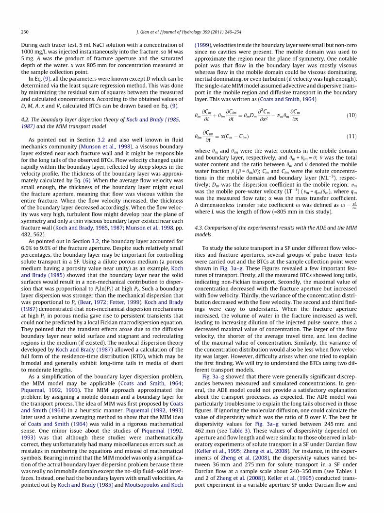
To study the solute transport in a SF under different flow veloc-ities and fracture apertures, several groups of pulse tracer testswere carried out and the BTCs at the sample collection point wereshown in Fig. 3a–g. These Figures revealed a few important fea-tures of transport. Firstly, all the measured BTCs showed long tails,indicating non-Fickian transport. Secondly, the maximal value ofconcentration decreased with the fracture aperture but increasedwith flow velocity. Thirdly, the variance of the concentration distri-bution decreased with the flow velocity. The second and third find-ings were easy to understand. When the fracture apertureincreased, the volume of water in the fracture increased as well,leading to increasing dilution of the injected pulse source, thus adecreased maximal value of concentration. The larger of the flowvelocity, the shorter of the average travel time, and less declineof the maximal value of concentration. Similarly, the variance ofthe concentration distribution would also be less when flow veloc-ity was larger. However, difficulty arises when one tried to explainthe first finding. We will try to understand the BTCs using two dif-ferent transport models.

Fig. 3a–g showed that there were generally significant discrep-ancies between measured and simulated concentrations. In gen-eral, the ADE model could not provide a satisfactory explanationabout the transport processes, as expected. The ADE model wasparticularly troublesome to explain the long tails observed in thosefigures. If ignoring the molecular diffusion, one could calculate thevalue of dispersivity which was the ratio of D over V. The best fitdispersivity values for Fig. 3a–g varied between 245 mm and462 mm (see Table 3). These values of dispersivity depended onaperture and flow length and were similar to those observed in lab-oratory experiments of solute transport in a SF under Darcian flow(Keller et al., 1995; Zheng et al., 2008). For instance, in the exper-iments of Zheng et al. (2008), the dispersivity values varied be-tween 36 mm and 275 mm for solute transport in a SF underDarcian flow at a sample scale about 240–350 mm (see Tables 1and 2 of Zheng et al. (2008)). Keller et al. (1995) conducted trans-port experiment in a variable aperture SF under Darcian flow and

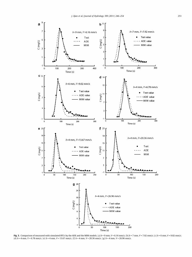
Fig. 3. Comparison of measured with simulated BTCs by the ADE and the MIM models. (a) b = 9 mm, V = 6.16 mm/s; (b) b = 7 mm, V = 7.92 mm/s; (c) b = 6 mm, V = 9.02 mm/s;(d) b = 4 mm, V = 6.78 mm/s; (e) b = 4 mm, V = 13.67 mm/s; (f) b = 4 mm, V = 20.36 mm/s; (g) b = 4 mm, V = 26.96 mm/s.

J. Qian et al. / Journal of Hydrology 399 (2011) 246–254 251

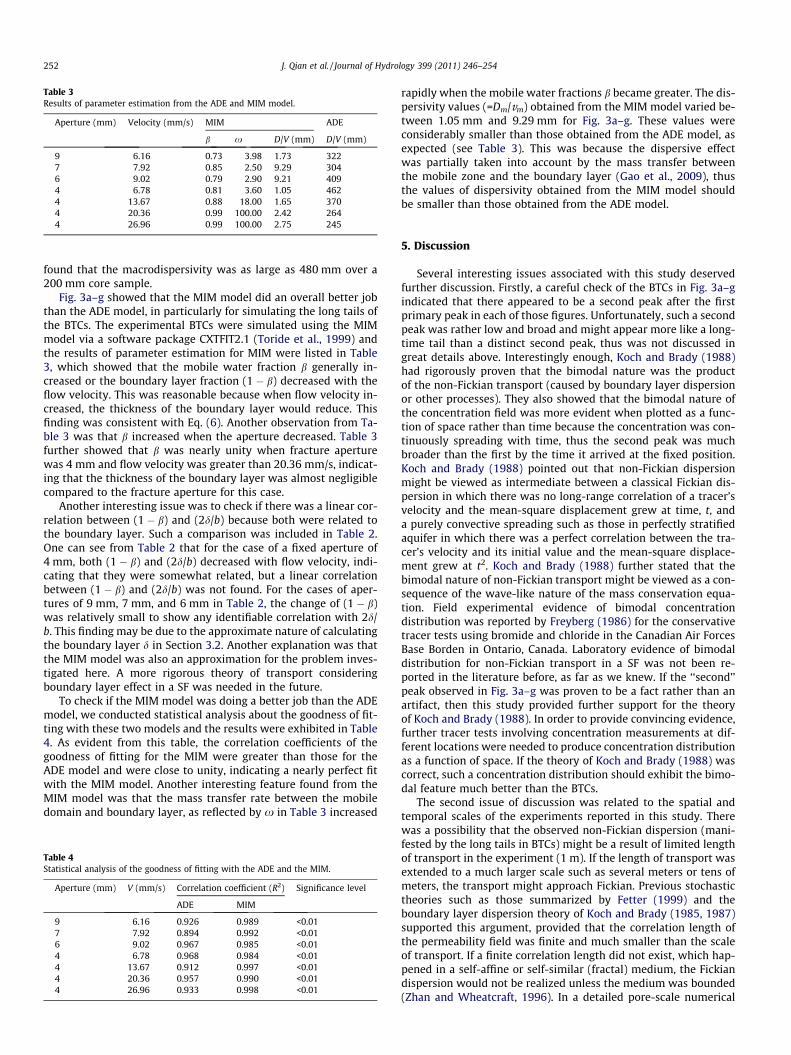
Table 3Results of parameter estimation from the ADE and MIM model.

Aperture (mm) Velocity (mm/s) MIM ADE

b x D/V (mm) D/V (mm)

9 6.16 0.73 3.98 1.73 3227 7.92 0.85 2.50 9.29 3046 9.02 0.79 2.90 9.21 4094 6.78 0.81 3.60 1.05 4624 13.67 0.88 18.00 1.65 3704 20.36 0.99 100.00 2.42 2644 26.96 0.99 100.00 2.75 245

252 J. Qian et al. / Journal of Hydrology 399 (2011) 246–254

found that the macrodispersivity was as large as 480 mm over a200 mm core sample.

Fig. 3a–g showed that the MIM model did an overall better jobthan the ADE model, in particularly for simulating the long tails ofthe BTCs. The experimental BTCs were simulated using the MIMmodel via a software package CXTFIT2.1 (Toride et al., 1999) andthe results of parameter estimation for MIM were listed in Table3, which showed that the mobile water fraction b generally in-creased or the boundary layer fraction (1 � b) decreased with theflow velocity. This was reasonable because when flow velocity in-creased, the thickness of the boundary layer would reduce. Thisfinding was consistent with Eq. (6). Another observation from Ta-ble 3 was that b increased when the aperture decreased. Table 3further showed that b was nearly unity when fracture aperturewas 4 mm and flow velocity was greater than 20.36 mm/s, indicat-ing that the thickness of the boundary layer was almost negligiblecompared to the fracture aperture for this case.

Another interesting issue was to check if there was a linear cor-relation between (1 � b) and (2d/b) because both were related tothe boundary layer. Such a comparison was included in Table 2.One can see from Table 2 that for the case of a fixed aperture of4 mm, both (1 � b) and (2d/b) decreased with flow velocity, indi-cating that they were somewhat related, but a linear correlationbetween (1 � b) and (2d/b) was not found. For the cases of aper-tures of 9 mm, 7 mm, and 6 mm in Table 2, the change of (1 � b)was relatively small to show any identifiable correlation with 2d/b. This finding may be due to the approximate nature of calculatingthe boundary layer d in Section 3.2. Another explanation was thatthe MIM model was also an approximation for the problem inves-tigated here. A more rigorous theory of transport consideringboundary layer effect in a SF was needed in the future.

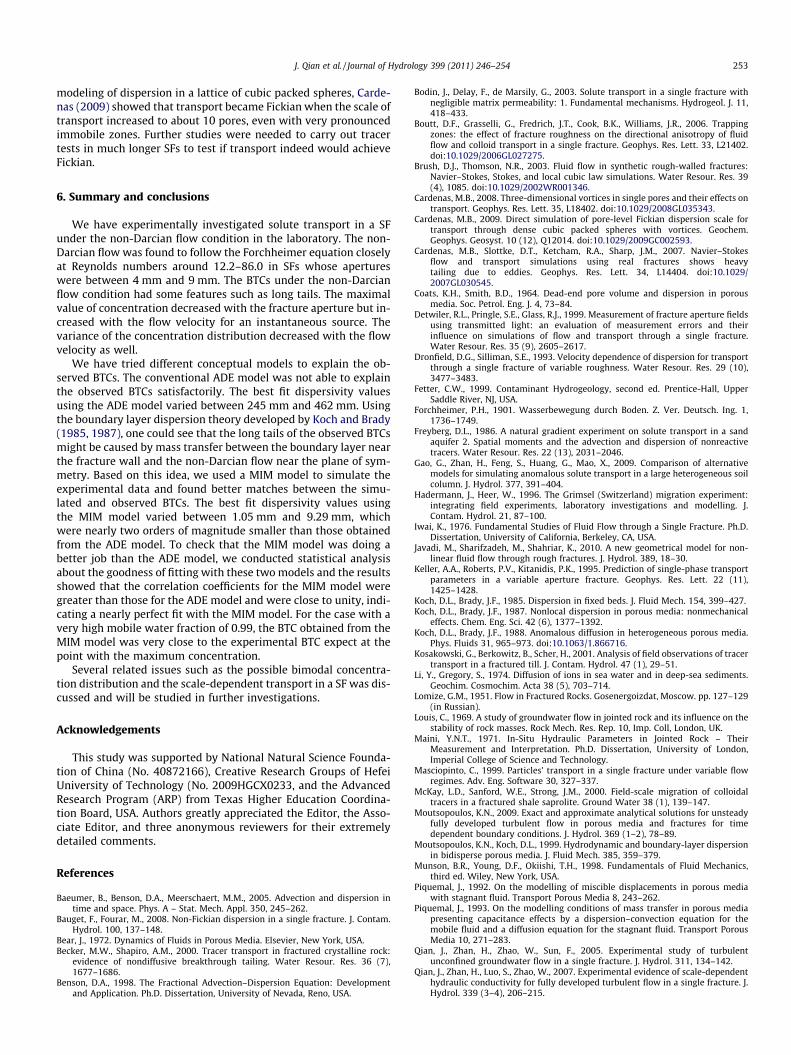
To check if the MIM model was doing a better job than the ADEmodel, we conducted statistical analysis about the goodness of fit-ting with these two models and the results were exhibited in Table4. As evident from this table, the correlation coefficients of thegoodness of fitting for the MIM were greater than those for theADE model and were close to unity, indicating a nearly perfect fitwith the MIM model. Another interesting feature found from theMIM model was that the mass transfer rate between the mobiledomain and boundary layer, as reflected by x in Table 3 increased

Table 4Statistical analysis of the goodness of fitting with the ADE and the MIM.

Aperture (mm) V (mm/s) Correlation coefficient (R2) Significance level

ADE MIM

9 6.16 0.926 0.989 <0.017 7.92 0.894 0.992 <0.016 9.02 0.967 0.985 <0.014 6.78 0.968 0.984 <0.014 13.67 0.912 0.997 <0.014 20.36 0.957 0.990 <0.014 26.96 0.933 0.998 <0.01

rapidly when the mobile water fractions b became greater. The dis-persivity values (=Dm/vm) obtained from the MIM model varied be-tween 1.05 mm and 9.29 mm for Fig. 3a–g. These values wereconsiderably smaller than those obtained from the ADE model, asexpected (see Table 3). This was because the dispersive effectwas partially taken into account by the mass transfer betweenthe mobile zone and the boundary layer (Gao et al., 2009), thusthe values of dispersivity obtained from the MIM model shouldbe smaller than those obtained from the ADE model.

5. Discussion

Several interesting issues associated with this study deservedfurther discussion. Firstly, a careful check of the BTCs in Fig. 3a–gindicated that there appeared to be a second peak after the firstprimary peak in each of those figures. Unfortunately, such a secondpeak was rather low and broad and might appear more like a long-time tail than a distinct second peak, thus was not discussed ingreat details above. Interestingly enough, Koch and Brady (1988)had rigorously proven that the bimodal nature was the productof the non-Fickian transport (caused by boundary layer dispersionor other processes). They also showed that the bimodal nature ofthe concentration field was more evident when plotted as a func-tion of space rather than time because the concentration was con-tinuously spreading with time, thus the second peak was muchbroader than the first by the time it arrived at the fixed position.Koch and Brady (1988) pointed out that non-Fickian dispersionmight be viewed as intermediate between a classical Fickian dis-persion in which there was no long-range correlation of a tracer’svelocity and the mean-square displacement grew at time, t, anda purely convective spreading such as those in perfectly stratifiedaquifer in which there was a perfect correlation between the tra-cer’s velocity and its initial value and the mean-square displace-ment grew at t2. Koch and Brady (1988) further stated that thebimodal nature of non-Fickian transport might be viewed as a con-sequence of the wave-like nature of the mass conservation equa-tion. Field experimental evidence of bimodal concentrationdistribution was reported by Freyberg (1986) for the conservativetracer tests using bromide and chloride in the Canadian Air ForcesBase Borden in Ontario, Canada. Laboratory evidence of bimodaldistribution for non-Fickian transport in a SF was not been re-ported in the literature before, as far as we knew. If the ‘‘second’’peak observed in Fig. 3a–g was proven to be a fact rather than anartifact, then this study provided further support for the theoryof Koch and Brady (1988). In order to provide convincing evidence,further tracer tests involving concentration measurements at dif-ferent locations were needed to produce concentration distributionas a function of space. If the theory of Koch and Brady (1988) wascorrect, such a concentration distribution should exhibit the bimo-dal feature much better than the BTCs.

The second issue of discussion was related to the spatial andtemporal scales of the experiments reported in this study. Therewas a possibility that the observed non-Fickian dispersion (mani-fested by the long tails in BTCs) might be a result of limited lengthof transport in the experiment (1 m). If the length of transport wasextended to a much larger scale such as several meters or tens ofmeters, the transport might approach Fickian. Previous stochastictheories such as those summarized by Fetter (1999) and theboundary layer dispersion theory of Koch and Brady (1985, 1987)supported this argument, provided that the correlation length ofthe permeability field was finite and much smaller than the scaleof transport. If a finite correlation length did not exist, which hap-pened in a self-affine or self-similar (fractal) medium, the Fickiandispersion would not be realized unless the medium was bounded(Zhan and Wheatcraft, 1996). In a detailed pore-scale numerical

J. Qian et al. / Journal of Hydrology 399 (2011) 246–254 253

modeling of dispersion in a lattice of cubic packed spheres, Carde-nas (2009) showed that transport became Fickian when the scale oftransport increased to about 10 pores, even with very pronouncedimmobile zones. Further studies were needed to carry out tracertests in much longer SFs to test if transport indeed would achieveFickian.

6. Summary and conclusions

We have experimentally investigated solute transport in a SFunder the non-Darcian flow condition in the laboratory. The non-Darcian flow was found to follow the Forchheimer equation closelyat Reynolds numbers around 12.2–86.0 in SFs whose apertureswere between 4 mm and 9 mm. The BTCs under the non-Darcianflow condition had some features such as long tails. The maximalvalue of concentration decreased with the fracture aperture but in-creased with the flow velocity for an instantaneous source. Thevariance of the concentration distribution decreased with the flowvelocity as well.

We have tried different conceptual models to explain the ob-served BTCs. The conventional ADE model was not able to explainthe observed BTCs satisfactorily. The best fit dispersivity valuesusing the ADE model varied between 245 mm and 462 mm. Usingthe boundary layer dispersion theory developed by Koch and Brady(1985, 1987), one could see that the long tails of the observed BTCsmight be caused by mass transfer between the boundary layer nearthe fracture wall and the non-Darcian flow near the plane of sym-metry. Based on this idea, we used a MIM model to simulate theexperimental data and found better matches between the simu-lated and observed BTCs. The best fit dispersivity values usingthe MIM model varied between 1.05 mm and 9.29 mm, whichwere nearly two orders of magnitude smaller than those obtainedfrom the ADE model. To check that the MIM model was doing abetter job than the ADE model, we conducted statistical analysisabout the goodness of fitting with these two models and the resultsshowed that the correlation coefficients for the MIM model weregreater than those for the ADE model and were close to unity, indi-cating a nearly perfect fit with the MIM model. For the case with avery high mobile water fraction of 0.99, the BTC obtained from theMIM model was very close to the experimental BTC expect at thepoint with the maximum concentration.

Several related issues such as the possible bimodal concentra-tion distribution and the scale-dependent transport in a SF was dis-cussed and will be studied in further investigations.

Acknowledgements

This study was supported by National Natural Science Founda-tion of China (No. 40872166), Creative Research Groups of HefeiUniversity of Technology (No. 2009HGCX0233, and the AdvancedResearch Program (ARP) from Texas Higher Education Coordina-tion Board, USA. Authors greatly appreciated the Editor, the Asso-ciate Editor, and three anonymous reviewers for their extremelydetailed comments.

References

Baeumer, B., Benson, D.A., Meerschaert, M.M., 2005. Advection and dispersion intime and space. Phys. A – Stat. Mech. Appl. 350, 245–262.

Bauget, F., Fourar, M., 2008. Non-Fickian dispersion in a single fracture. J. Contam.Hydrol. 100, 137–148.

Bear, J., 1972. Dynamics of Fluids in Porous Media. Elsevier, New York, USA.Becker, M.W., Shapiro, A.M., 2000. Tracer transport in fractured crystalline rock:

evidence of nondiffusive breakthrough tailing. Water Resour. Res. 36 (7),1677–1686.

Benson, D.A., 1998. The Fractional Advection–Dispersion Equation: Developmentand Application. Ph.D. Dissertation, University of Nevada, Reno, USA.

Bodin, J., Delay, F., de Marsily, G., 2003. Solute transport in a single fracture withnegligible matrix permeability: 1. Fundamental mechanisms. Hydrogeol. J. 11,418–433.

Boutt, D.F., Grasselli, G., Fredrich, J.T., Cook, B.K., Williams, J.R., 2006. Trappingzones: the effect of fracture roughness on the directional anisotropy of fluidflow and colloid transport in a single fracture. Geophys. Res. Lett. 33, L21402.doi:10.1029/2006GL027275.

Brush, D.J., Thomson, N.R., 2003. Fluid flow in synthetic rough-walled fractures:Navier–Stokes, Stokes, and local cubic law simulations. Water Resour. Res. 39(4), 1085. doi:10.1029/2002WR001346.

Cardenas, M.B., 2008. Three-dimensional vortices in single pores and their effects ontransport. Geophys. Res. Lett. 35, L18402. doi:10.1029/2008GL035343.

Cardenas, M.B., 2009. Direct simulation of pore-level Fickian dispersion scale fortransport through dense cubic packed spheres with vortices. Geochem.Geophys. Geosyst. 10 (12), Q12014. doi:10.1029/2009GC002593.

Cardenas, M.B., Slottke, D.T., Ketcham, R.A., Sharp, J.M., 2007. Navier–Stokesflow and transport simulations using real fractures shows heavytailing due to eddies. Geophys. Res. Lett. 34, L14404. doi:10.1029/2007GL030545.

Coats, K.H., Smith, B.D., 1964. Dead-end pore volume and dispersion in porousmedia. Soc. Petrol. Eng. J. 4, 73–84.

Detwiler, R.L., Pringle, S.E., Glass, R.J., 1999. Measurement of fracture aperture fieldsusing transmitted light: an evaluation of measurement errors and theirinfluence on simulations of flow and transport through a single fracture.Water Resour. Res. 35 (9), 2605–2617.

Dronfield, D.G., Silliman, S.E., 1993. Velocity dependence of dispersion for transportthrough a single fracture of variable roughness. Water Resour. Res. 29 (10),3477–3483.

Fetter, C.W., 1999. Contaminant Hydrogeology, second ed. Prentice-Hall, UpperSaddle River, NJ, USA.

Forchheimer, P.H., 1901. Wasserbewegung durch Boden. Z. Ver. Deutsch. Ing. 1,1736–1749.

Freyberg, D.L., 1986. A natural gradient experiment on solute transport in a sandaquifer 2. Spatial moments and the advection and dispersion of nonreactivetracers. Water Resour. Res. 22 (13), 2031–2046.

Gao, G., Zhan, H., Feng, S., Huang, G., Mao, X., 2009. Comparison of alternativemodels for simulating anomalous solute transport in a large heterogeneous soilcolumn. J. Hydrol. 377, 391–404.

Hadermann, J., Heer, W., 1996. The Grimsel (Switzerland) migration experiment:integrating field experiments, laboratory investigations and modelling. J.Contam. Hydrol. 21, 87–100.

Iwai, K., 1976. Fundamental Studies of Fluid Flow through a Single Fracture. Ph.D.Dissertation, University of California, Berkeley, CA, USA.

Javadi, M., Sharifzadeh, M., Shahriar, K., 2010. A new geometrical model for non-linear fluid flow through rough fractures. J. Hydrol. 389, 18–30.

Keller, A.A., Roberts, P.V., Kitanidis, P.K., 1995. Prediction of single-phase transportparameters in a variable aperture fracture. Geophys. Res. Lett. 22 (11),1425–1428.

Koch, D.L., Brady, J.F., 1985. Dispersion in fixed beds. J. Fluid Mech. 154, 399–427.Koch, D.L., Brady, J.F., 1987. Nonlocal dispersion in porous media: nonmechanical

effects. Chem. Eng. Sci. 42 (6), 1377–1392.Koch, D.L., Brady, J.F., 1988. Anomalous diffusion in heterogeneous porous media.

Phys. Fluids 31, 965–973. doi:10.1063/1.866716.Kosakowski, G., Berkowitz, B., Scher, H., 2001. Analysis of field observations of tracer

transport in a fractured till. J. Contam. Hydrol. 47 (1), 29–51.Li, Y., Gregory, S., 1974. Diffusion of ions in sea water and in deep-sea sediments.

Geochim. Cosmochim. Acta 38 (5), 703–714.Lomize, G.M., 1951. Flow in Fractured Rocks. Gosenergoizdat, Moscow. pp. 127–129

(in Russian).Louis, C., 1969. A study of groundwater flow in jointed rock and its influence on the

stability of rock masses. Rock Mech. Res. Rep. 10, Imp. Coll, London, UK.Maini, Y.N.T., 1971. In-Situ Hydraulic Parameters in Jointed Rock – Their

Measurement and Interpretation. Ph.D. Dissertation, University of London,Imperial College of Science and Technology.

Masciopinto, C., 1999. Particles’ transport in a single fracture under variable flowregimes. Adv. Eng. Software 30, 327–337.

McKay, L.D., Sanford, W.E., Strong, J.M., 2000. Field-scale migration of colloidaltracers in a fractured shale saprolite. Ground Water 38 (1), 139–147.

Moutsopoulos, K.N., 2009. Exact and approximate analytical solutions for unsteadyfully developed turbulent flow in porous media and fractures for timedependent boundary conditions. J. Hydrol. 369 (1–2), 78–89.

Moutsopoulos, K.N., Koch, D.L., 1999. Hydrodynamic and boundary-layer dispersionin bidisperse porous media. J. Fluid Mech. 385, 359–379.

Munson, B.R., Young, D.F., Okiishi, T.H., 1998. Fundamentals of Fluid Mechanics,third ed. Wiley, New York, USA.

Piquemal, J., 1992. On the modelling of miscible displacements in porous mediawith stagnant fluid. Transport Porous Media 8, 243–262.

Piquemal, J., 1993. On the modelling conditions of mass transfer in porous mediapresenting capacitance effects by a dispersion–convection equation for themobile fluid and a diffusion equation for the stagnant fluid. Transport PorousMedia 10, 271–283.

Qian, J., Zhan, H., Zhao, W., Sun, F., 2005. Experimental study of turbulentunconfined groundwater flow in a single fracture. J. Hydrol. 311, 134–142.

Qian, J., Zhan, H., Luo, S., Zhao, W., 2007. Experimental evidence of scale-dependenthydraulic conductivity for fully developed turbulent flow in a single fracture. J.Hydrol. 339 (3–4), 206–215.

254 J. Qian et al. / Journal of Hydrology 399 (2011) 246–254

Qian, J., Chen, Z., Zhan, H., Guan, H., 2010. Experimental study of the effect ofroughness and Reynolds number on fluid flow in rough-walled single fractures:A check of local cubic law. Hydrol. Process. 24, doi:10.1002/hyp.7849.

Qian, J., Chen, Z., Zhan, H., Luo, S., 2011. Solute transport in a filled single fractureunder non-Darcian flow. Int. J. Rock Mech. Mining Sci. 48, 132–140.doi:10.1016/j.ijrmms.2010.09.009.

Scher, H., Lax, M., 1973. Stochastic transport in a disordered solid. 1. Theory. Phys.Rev. B 7 (10), 4491–4502.

Sharp, J.C., Maini, Y.N.T., 1972. Fundamental considerations on the hydrauliccharacteristics of joints in rock. In: Proceedings Symposium on Percolationthrough Fissured Rock, International Society for Rock Mechanics, Stuttgart, n.T1-F.

Sidle, R.C., Nilsson, B., Hansen, M., Fredericia, J., 1998. Spatially varying hydraulicand solute transport characteristics of a fractured till determined by field tracertests, Funen, Denmark. Water Resour. Res. 34 (10), 2515–2527.

Toride, N., Leij, F., van Genuchten, M.Th., 1999. The CXTFIT Code for EstimatingTransport Parameters from Laboratory or Field Tracer Experiments, Version 2.1.US Salinity Lab Research Rep. 137, US Salinity Lab, Riverside, CA, USA.

Wen, Z., Huang, G., Zhan, H., 2006. Non-Darcian flow in a single confined verticalfracture toward a well. J. Hydrol. 330 (3–4), 698–708.

Witherspoon, P.A., Wang, J.S.Y., Iwai, K., Gale, J.E., 1980. Validity of cubic law forfluid flow in a deformable rock fracture. Water Resour. Res. 16 (6), 1016–1024.

Zhan, H., 1998. Transport of waste leakage in stratified formations. Adv. WaterResour. 22 (2), 159–168.

Zhan, H., Wheatcraft, S.W., 1996. Macrodispersivity tensor for nonreactive solutetransport in isotropic and anisotropic fractal porous media: analytical solutions.Water Resour. Res. 32 (12), 3461–3474.

Zheng, Q., Dickson, S.E., Guo, Y., 2008. On the appropriate ‘‘equivalent aperture’’ forthe description of solute transport in single fractures: laboratory-scaleexperiments. Water Resour. Res. 44, W04502. doi:10.1029/2007WR005970.

Zimmerman, R.W., Yeo, I.W., 2000. Fluid flow in rock fractures: from the Navier–Stokes equations to the cubic law. In: Faybishenko, B., Witherspoon, P.A.,Benson, S.M. (Eds.), Dynamics of Fluids in Fractured Rock. AmericanGeophysical Union Monograph 122, Washington, DC, USA, pp. 213–224.