HAL Id: hal-00631562https://hal.archives-ouvertes.fr/hal-00631562v2

Submitted on 26 Jul 2012 (v2), last revised 20 Nov 2012 (v3)

HAL is a multi-disciplinary open accessarchive for the deposit and dissemination of sci-entific research documents, whether they are pub-lished or not. The documents may come fromteaching and research institutions in France orabroad, or from public or private research centers.

L’archive ouverte pluridisciplinaire HAL, estdestinée au dépôt et à la diffusion de documentsscientifiques de niveau recherche, publiés ou non,émanant des établissements d’enseignement et derecherche français ou étrangers, des laboratoirespublics ou privés.

Experimental study of hydraulic transport of largeparticles in horizontal pipes

Florent Ravelet, Farid Bakir, Sofiane Khelladi, Robert Rey

To cite this version:Florent Ravelet, Farid Bakir, Sofiane Khelladi, Robert Rey. Experimental study of hydraulic transportof large particles in horizontal pipes. 2012. <hal-00631562v2>

Experimental study of hydraulic transport of large particles in horizontal pipes

F. Raveleta,∗, F. Bakira, S. Khelladia, R. Reya

aArts et Metiers ParisTech, DynFluid, 151 boulevard de l’Hopital, 75013 Paris, France.

Abstract

This article presents an experimental study of the hydraulic transport of very large solid particles (above 5 mm) in anhorizontal pipe. Two specific masses are used for the solids. The solids are spheres that are large with respect to thediameter of the pipe (5, 10 and 15%) or real stones of arbitrary shapes but constant specific mass and a size distributionsimilar to the tested spherical beads. Finally, mixtures of size and / or specific mass are studied. The regimes arecharacterized with differential pressure measurements and visualizations. The results are compared to empirical modelsbased on dimensionless numbers, together with 1D models that are based on mass and momentum balance. A modelfor the transport of large particles in vertical pipes is also proposed and tested on data available in the Literature, inorder to compare the trends that are observed in the present experiments in a horizontal pipe to the trends predictedfor a vertical pipe. The results show that the grain size and specific mass have a strong effect on the transition pointbetween regimes with a stationary bed and dispersed flows. The pressure drops are moreover smaller for large particlesin the horizontal part contrary to what occurs for vertical pipes, and to the predictions of the empirical correlations.

Keywords: Hydraulic transport, solid-liquid two-phase flow, bed friction, deep sea mining.

1. Introduction

The hydraulic transport of solid particles is a methodwidely used in chemical and mining industries. Many pre-dictive models exist in the case of suspensions, that is tosay when the particle diameter is small compared to theflow length scales and the velocity of the carrier fluid ishigh compared to the settling velocity of a particle [1–4]. It is then possible to predict the pressure losses inhorizontal or vertical pipes with sufficient accuracy. In re-cent years, the sharp increase in demand for raw materialsmakes it interesting exploitation of new resources, partic-ularly the use of fields at the bottom of the ocean [5, 6].In this case, the solids may be large with respect to thepipe diameter and the circuit would have complex shapes,including vertical parts, horizontal parts, and potentiallybends and S-shapes in order to absorb the deformationscaused by surface waves. For transport of large parti-cles in vertical pipe, a predictive model based on the workof Newitt et al. [7] and Richardson et al. [8] is proposedand validated on a set of experimental data [9–11]. How-ever, in horizontal, and a fortiori in geometries in S-shape,there are few models [1–4, 12–15] and the effects of specificmass and more specifically of very large particle size havenot been systematically explored. One major difficulty inthe case of transport of large particles and high specificmass comes from the various flow regimes that may beobserved [1, 2, 4, 12, 13, 16, 17]: when the speed of trans-portation increases, several transitions arise from regimes

∗corresponding authorEmail address: florent.ravelet@ensta.org (F. Ravelet)

with a layer of solids at the bottom of the pipe that is atrest or that flows backwards in inclined pipes [13, 16, 17]to regimes with a moving bed and eventually to heteroge-neous and pseudo-homogeneous suspensions at high mix-ture velocities.

The knowledge of the velocity above which the bedstarts to move forward is of great interest with respect tooperation of a production line. Below this limit the systemmay indeed plug. In the present study, experiments arecarried out in order to better understand the effects ofsolid size and specific mass on this velocity and on thepressure drop.

The experimental set-up is presented in § 2. Somegeneral considerations on the typical regimes and pressuredrop curves that are specific to an horizontal pipe and anoverview of the state of the art are presented in § 3. Theexperimental results are presented and discussed in § 4.The main results that concern mono-disperse calibratedsolid spheres of two different sizes and two different spe-cific masses flowing in the horizontal pipe are presentedin § 4.1. Mixture of spheres and rough stones of arbi-trary shapes are also tested in § 4.2, in order to check towhat extent the results obtained for spheres may repre-sent an actual application. Several models are proposedand compared to the experiments in § 4.3. Conclusionsand perspectives are then given in § 5.

Preprint submitted to Experimental Thermal and Fluid Science July 26, 2012

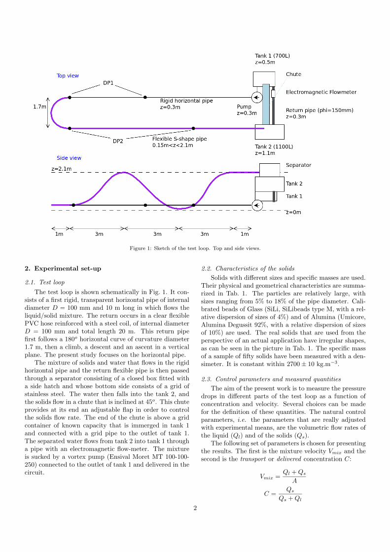
Figure 1: Sketch of the test loop. Top and side views.

2. Experimental set-up

2.1. Test loop

The test loop is shown schematically in Fig. 1. It con-sists of a first rigid, transparent horizontal pipe of internaldiameter D = 100 mm and 10 m long in which flows theliquid/solid mixture. The return occurs in a clear flexiblePVC hose reinforced with a steel coil, of internal diameterD = 100 mm and total length 20 m. This return pipefirst follows a 180o horizontal curve of curvature diameter1.7 m, then a climb, a descent and an ascent in a verticalplane. The present study focuses on the horizontal pipe.

The mixture of solids and water that flows in the rigidhorizontal pipe and the return flexible pipe is then passedthrough a separator consisting of a closed box fitted witha side hatch and whose bottom side consists of a grid ofstainless steel. The water then falls into the tank 2, andthe solids flow in a chute that is inclined at 45o. This chuteprovides at its end an adjustable flap in order to controlthe solids flow rate. The end of the chute is above a gridcontainer of known capacity that is immerged in tank 1and connected with a grid pipe to the outlet of tank 1.The separated water flows from tank 2 into tank 1 througha pipe with an electromagnetic flow-meter. The mixtureis sucked by a vortex pump (Ensival Moret MT 100-100-250) connected to the outlet of tank 1 and delivered in thecircuit.

2.2. Characteristics of the solids

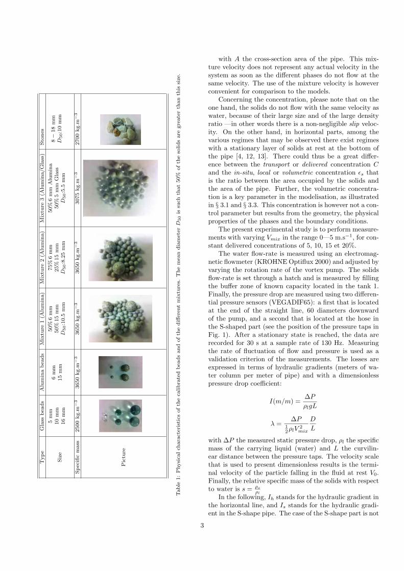
Solids with different sizes and specific masses are used.Their physical and geometrical characteristics are summa-rized in Tab. 1. The particles are relatively large, withsizes ranging from 5% to 18% of the pipe diameter. Cali-brated beads of Glass (SiLi, SiLibeads type M, with a rel-ative dispersion of sizes of 4%) and of Alumina (Umicore,Alumina Degussit 92%, with a relative dispersion of sizesof 10%) are used. The real solids that are used from theperspective of an actual application have irregular shapes,as can be seen in the picture in Tab. 1. The specific massof a sample of fifty solids have been measured with a den-simeter. It is constant within 2700± 10 kg.m−3.

2.3. Control parameters and measured quantities

The aim of the present work is to measure the pressuredrops in different parts of the test loop as a function ofconcentration and velocity. Several choices can be madefor the definition of these quantities. The natural controlparameters, i.e. the parameters that are really adjustedwith experimental means, are the volumetric flow rates ofthe liquid (Ql) and of the solids (Qs).

The following set of parameters is chosen for presentingthe results. The first is the mixture velocity Vmix and thesecond is the transport or delivered concentration C:

Vmix =Ql +Qs

A

C =Qs

Qs +Ql

2

Typ

eG

lass

bea

ds

Alu

min

ab

ead

sM

ixtu

re1

(Alu

min

a)

Mix

ture

2(A

lum

ina)

Mix

ture

3(A

lum

ina/G

lass

)S

ton

es

Siz

e

5m

m10

mm

16

mm

6m

m15

mm

50%

6m

m50%

15

mm

D50:1

0.5

mm

75%

6m

m25%

15

mm

D50:8.2

5m

m

50%

6m

mA

lum

ina

50%

5m

mG

lass

D50:5.5

mm

8−

18

mm

D50:1

0m

m

Sp

ecifi

cm

ass

2500

kg.m

−3

3650

kg.m

−3

3650

kg.m

−3

3650

kg.m

−3

3075

kg.m

−3

2700

kg.m

−3

Pic

ture

Tab

le1:

Physi

cal

chara

cter

isti

csof

the

calib

rate

db

ead

san

dof

the

diff

eren

tm

ixtu

res.

Th

em

ean

dia

met

erD

50

issu

chth

at

50%

of

the

solid

sare

gre

ate

rth

an

this

size

.

with A the cross-section area of the pipe. This mix-ture velocity does not represent any actual velocity in thesystem as soon as the different phases do not flow at thesame velocity. The use of the mixture velocity is howeverconvenient for comparison to the models.

Concerning the concentration, please note that on theone hand, the solids do not flow with the same velocity aswater, because of their large size and of the large densityratio —in other words there is a non-negligible slip veloc-ity. On the other hand, in horizontal parts, among thevarious regimes that may be observed there exist regimeswith a stationary layer of solids at rest at the bottom ofthe pipe [4, 12, 13]. There could thus be a great differ-ence between the transport or delivered concentration Cand the in-situ, local or volumetric concentration εs thatis the ratio between the area occupied by the solids andthe area of the pipe. Further, the volumetric concentra-tion is a key parameter in the modelisation, as illustratedin § 3.1 and § 3.3. This concentration is however not a con-trol parameter but results from the geometry, the physicalproperties of the phases and the boundary conditions.

The present experimental study is to perform measure-ments with varying Vmix in the range 0—5 m.s−1, for con-stant delivered concentrations of 5, 10, 15 et 20%.

The water flow-rate is measured using an electromag-netic flowmeter (KROHNE Optiflux 2000) and adjusted byvarying the rotation rate of the vortex pump. The solidsflow-rate is set through a hatch and is measured by fillingthe buffer zone of known capacity located in the tank 1.Finally, the pressure drop are measured using two differen-tial pressure sensors (VEGADIF65): a first that is locatedat the end of the straight line, 60 diameters downwardof the pump, and a second that is located at the hose inthe S-shaped part (see the position of the pressure taps inFig. 1). After a stationary state is reached, the data arerecorded for 30 s at a sample rate of 130 Hz. Measuringthe rate of fluctuation of flow and pressure is used as avalidation criterion of the measurements. The losses areexpressed in terms of hydraulic gradients (meters of wa-ter column per meter of pipe) and with a dimensionlesspressure drop coefficient:

I(m/m) =∆P

ρlgL

λ =∆P

12ρlV

2mix

D

L

with ∆P the measured static pressure drop, ρl the specificmass of the carrying liquid (water) and L the curvilin-ear distance between the pressure taps. The velocity scalethat is used to present dimensionless results is the termi-nal velocity of the particle falling in the fluid at rest V0.Finally, the relative specific mass of the solids with respectto water is s = ρs

ρlIn the following, Ih stands for the hydraulic gradient in

the horizontal line, and Is stands for the hydraulic gradi-ent in the S-shape pipe. The case of the S-shape part is not

3

fully developed here and will be discussed in a forthcomingpaper with new experimental data including a better dis-cretisation of the different inclined parts and bends. Thesymbol Iv is used for the hydraulic gradient that would beobserved in a vertical pipe.

Optical measurements are also performed with a high-speed camera (Optronis CamRecord600). Typically 3200images are recorded with a resolution of 1280×1024 pixelsat a frame rate of 200 Hz. The flow is illuminated back-wards with a LED plate from Phlox. The visualizationarea is surrounded by a square plexiglas box filled withwater in order to minimize optical distorsions.

3. Overview of the state of the art and of the ob-served regimes

A common feature of multiphase flows is the existenceof very different flow patterns, which makes modeling muchmore complicated. In the case of solid transport, severalstratified and dispersed regimes are observed in horizon-tal and inclined flows [1, 2, 4, 17], whereas only dispersedregimes arise in vertical flows [2, 9–11]. The present sec-tion first presents a model for vertical flows and then thetypical regimes that are encountered in the horizontal ex-periment and the different possible models.

3.1. Validation of a model for the transport of large parti-cles in vertical pipelines

The case of vertical flow is reasonably straightforward.The pressure force exerted on a column of fluid of heightz balances two forces: the hydrostatic weight of the mix-ture and the friction on pipe wall due to the fluid shearstress [1, 2]. In the following, the hydrostatic weight ofthe column of water is removed in order to present thehydraulic gradients that are due to the flow of a mixturein the pipe.

The vertical hydraulic gradient Iv can thus be decom-posed into two parts: Iv = Istat + If , with Istat the hy-drostatic contribution and If the wall shear-stress contri-bution. The hydrostatic contribution reads:

Istat = (s− 1)εs

The in-situ concentration εs is a priori unknown. Fol-lowing the seminal work of Newitt et al. [7], the averagevelocity difference between the solids and the surroundingwater, or slip velocity Vslip reads:

Vslip =1− C1− εs

Vmix −C

εsVmix (1)

This slip velocity would be the terminal velocity V0for a single solid of diameter dp and of drag coefficientcd = 0.44 falling in an infinite medium of fluid at rest:

V0 =

√4dpg(s− 1)

3cd(2)

0 2 4 6 8 1010

−2

10−1

100

Vmix

/V0

λv

(b)

0 1 2 3 4 5 6 70

0.1

0.2

0.3

0.4

0.5

0.6

Vmix

(m.s−1

)

I v (

m/m

)

(a)

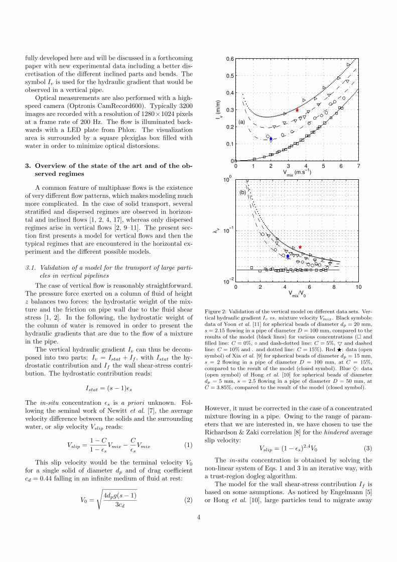
Figure 2: Validation of the vertical model on different data sets. Ver-tical hydraulic gradient Iv vs. mixture velocity Vmix. Black symbols:data of Yoon et al. [11] for spherical beads of diameter dp = 20 mm,s = 2.15 flowing in a pipe of diameter D = 100 mm, compared to theresults of the model (black lines) for various concentrations (� andfilled line: C = 0%, ◦ and dash-dotted line: C = 5%, 5 and dashedline: C = 10% and . and dotted line: C = 15%). Red F: data (opensymbol) of Xia et al. [9] for spherical beads of diameter dp = 15 mm,s = 2 flowing in a pipe of diameter D = 100 mm, at C = 15%,compared to the result of the model (closed symbol). Blue ♦: data(open symbol) of Hong et al. [10] for spherical beads of diameterdp = 5 mm, s = 2.5 flowing in a pipe of diameter D = 50 mm, atC = 3.85%, compared to the result of the model (closed symbol).

However, it must be corrected in the case of a concentratedmixture flowing in a pipe. Owing to the range of param-eters that we are interested in, we have chosen to use theRichardson & Zaki correlation [8] for the hindered averageslip velocity:

Vslip = (1− εs)2.4V0 (3)

The in-situ concentration is obtained by solving thenon-linear system of Eqs. 1 and 3 in an iterative way, witha trust-region dogleg algorithm.

The model for the wall shear-stress contribution If isbased on some asumptions. As noticed by Engelmann [5]or Hong et al. [10], large particles tend to migrate away

4

from the wall due to hydrodynamic lift [2]. Assuming thatthe near-wall velocity profile is only slightly affected bythe presence of particles in the core region, the wall shear-stress is modeled by water flowing at the water velocity:

If = λ(Vmix

1−C1−εs )2

2gD

This model for vertical flow has been validated on var-ious experimental data available in the Literature [9–11].The comparison between the model and the data is plot-ted in Fig. 2. The agreement is very good. When dealingwith a mixture of liquid and solids, the pressure dropsare significantly higher than for pure fluid for the wholerange of mixture velocity that corresponds here to V0 ≤Vmix ≤ 8V0: it is for instance twice as large at C = 5%and Vmix = 4V0 for the beads of diameter dp = 0.2D ands = 2.15 (data of Yoon et al. [11], ◦ in Fig. 2). A re-markable feature of the curves is the presence of a localminimum: the hydraulic gradient does not vary monoton-ically with the velocity. This is due to the fact that thehydrostatic gradient is the dominant term and that it isa decreasing function of the mixture velocity. The in situconcentration εs is indeed much larger than the deliveredconcentration C and decreases with increasing Vmix. Forinstance, for the data plotted with ◦ in Fig. 2, εs = 13%for Vmix = V0, εs = 11% for Vmix = 1.2V0 = 1 m.s−1,εs = 10% = 2C for Vmix = 1.4V0 and εs = 6% forVmix = 4V0. The velocity which corresponds to the min-imum of the pressure drop curve (Vmix ' 1.8V0 for ◦ inFig. 2) is of great practical importance and the line shouldnot be operated below this velocity.

The model is thus used with the parameters of thepresent experiments to compare the order of magnitudeof hydraulic gradients and critical velocities between hori-zontal and vertical flows (see for instance Figs. 3 and 4b).

3.2. Description of the typical regimes in horizontal pipes

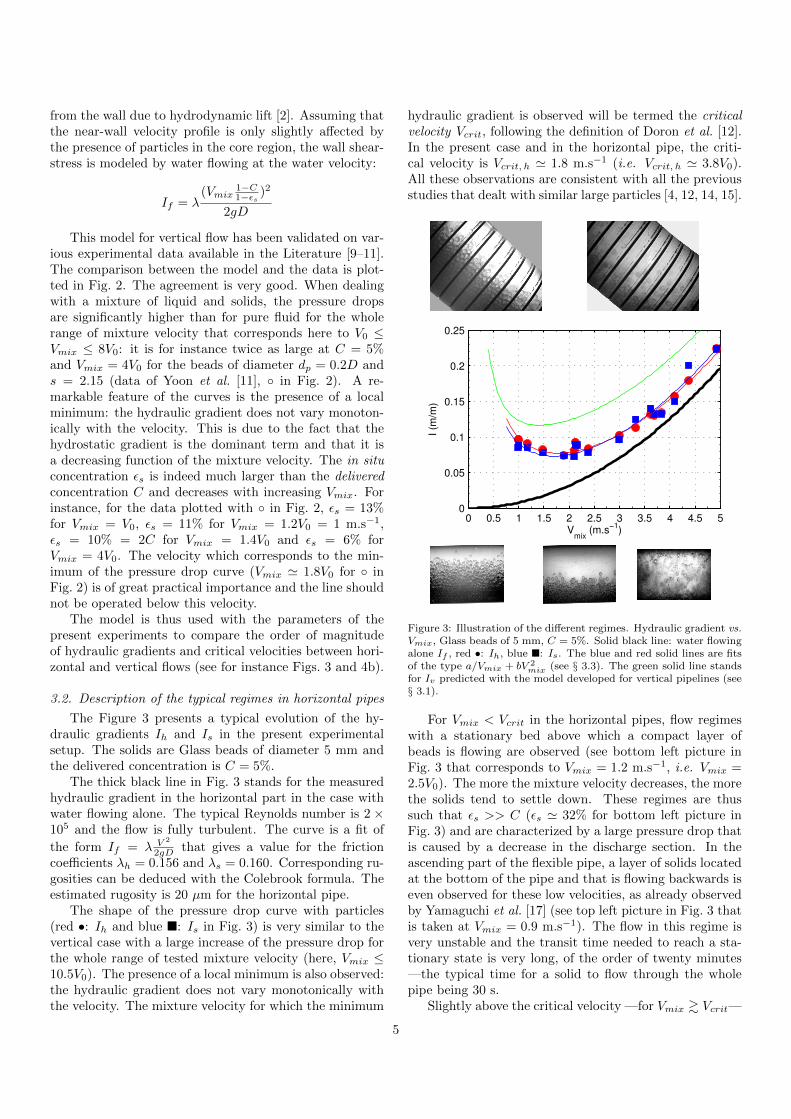
The Figure 3 presents a typical evolution of the hy-draulic gradients Ih and Is in the present experimentalsetup. The solids are Glass beads of diameter 5 mm andthe delivered concentration is C = 5%.

The thick black line in Fig. 3 stands for the measuredhydraulic gradient in the horizontal part in the case withwater flowing alone. The typical Reynolds number is 2 ×105 and the flow is fully turbulent. The curve is a fit of

the form If = λ V 2

2gD that gives a value for the frictioncoefficients λh = 0.156 and λs = 0.160. Corresponding ru-gosities can be deduced with the Colebrook formula. Theestimated rugosity is 20 µm for the horizontal pipe.

The shape of the pressure drop curve with particles(red •: Ih and blue �: Is in Fig. 3) is very similar to thevertical case with a large increase of the pressure drop forthe whole range of tested mixture velocity (here, Vmix ≤10.5V0). The presence of a local minimum is also observed:the hydraulic gradient does not vary monotonically withthe velocity. The mixture velocity for which the minimum

hydraulic gradient is observed will be termed the criticalvelocity Vcrit, following the definition of Doron et al. [12].In the present case and in the horizontal pipe, the criti-cal velocity is Vcrit, h ' 1.8 m.s−1 (i.e. Vcrit, h ' 3.8V0).All these observations are consistent with all the previousstudies that dealt with similar large particles [4, 12, 14, 15].

0 0.5 1 1.5 2 2.5 3 3.5 4 4.5 50

0.05

0.1

0.15

0.2

0.25

Vmix

(m.s−1

)

I (m

/m)

Figure 3: Illustration of the different regimes. Hydraulic gradient vs.Vmix, Glass beads of 5 mm, C = 5%. Solid black line: water flowingalone If , red •: Ih, blue �: Is. The blue and red solid lines are fitsof the type a/Vmix + bV 2

mix (see § 3.3). The green solid line standsfor Iv predicted with the model developed for vertical pipelines (see§ 3.1).

For Vmix < Vcrit in the horizontal pipes, flow regimeswith a stationary bed above which a compact layer ofbeads is flowing are observed (see bottom left picture inFig. 3 that corresponds to Vmix = 1.2 m.s−1, i.e. Vmix =2.5V0). The more the mixture velocity decreases, the morethe solids tend to settle down. These regimes are thussuch that εs >> C (εs ' 32% for bottom left picture inFig. 3) and are characterized by a large pressure drop thatis caused by a decrease in the discharge section. In theascending part of the flexible pipe, a layer of solids locatedat the bottom of the pipe and that is flowing backwards iseven observed for these low velocities, as already observedby Yamaguchi et al. [17] (see top left picture in Fig. 3 thatis taken at Vmix = 0.9 m.s−1). The flow in this regime isvery unstable and the transit time needed to reach a sta-tionary state is very long, of the order of twenty minutes—the typical time for a solid to flow through the wholepipe being 30 s.

Slightly above the critical velocity —for Vmix & Vcrit—

5

a bed on the bottom of the pipe that is sliding is observedboth in the horizontal pipe and in the S-shaped part (seebottom central picture and top right picture in Fig. 3 thatare both taken at Vmix = 2.1 m.s−1, i.e. Vmix = 4.1V0).The velocity of this bed is small compared to the mixturevelocity and εs > C here, εs ' 10%.

Increasing further the mixture velocity, more and moresolid beads get suspended and transported by the flow,there is no more bed, the flow is fully dispersed. Thepressure drop curves behave as the clear-water pressuredrop curve and follow the same trend at high velocities.In that case, εs & C and the regime is called “pseudo-homogeneous”[12] or “heterogeneous”[4] (see bottom rightpicture in Fig. 3 that is taken at Vmix = 4.9 m.s−1, i.e.Vmix = 10.3V0).

The green line is the results of the model for pressuredrop in vertical flow, presented in § 3.1. The main conclu-sions are first that the hydraulic gradient in the horizontalpart is lower than the one that would be observed in avertical pipe at least for this specific mass and solid size.The main contribution in the vertical model comes fromthe hydrostatic pressure of the mixture that is thus greaterthan the contribution of the bed formation in horizontalconfiguration. Secondly, the critical velocity in the hor-izontal pipe is greater than that of a vertical pipe. Theeffects of size, concentration and specific mass will be fur-ther explored in § 4.

3.3. Correlations and models

This paragraph is a brief overview of some of the cor-relations and models that are commonly used.

Empirical correlations. The first quantity of interest to bepresented is the critical velocity Vcrit. One correlation hasbeen proposed by Durand & Condolios (1952) [14]:

Vcrit = Fl{2Dg (s− 1)}1/2 (4)

with Fl a constant of order unity, that depends on thedelivered concentration and the particle size.

Concerning the prediction of the hydraulic gradient, afirst empirical correlation is the one proposed by Durand& coworkers [15]. They used sand particles of one spe-cific mass with diameter up to 25.4 mm in pipes rangingfrom 38 mm to 558 mm in diameter (the maximum relativediameter in the pipe of 104 mm was 4.5%). The dimen-sionless excess of pressure drop caused by the presence ofthe particles

Φ =Ih − IfIf

is expressed using two dimensionless groups:

FD = Vmix/√gD

a “Froude” number based on the mixture velocity and thepipe diameter and

Fdp = V0/√gdp

a “Froude” number based on the terminal velocity and thesize of the particle. These two parameters are grouped toform Ψ = F 2

DF−1dp

. They found a general correlation thatbest represents all their data:

Φ = 180C (Ψ)−1.5

(5)

It is recommended to use this correlation in the vicinityof the critical velocity (from mixture velocities slightly be-low to three or four times greater). This correlation wasthen modified to take into account the specific mass of theparticles, as reported by Newitt et al. [4]. In the case ofparticles of a few millimeters flowing in water, the particleReynolds number is sufficiently high to assume that thesettling velocity is given by Eq. 2 with a constant dragcoefficient cd. This form of the correlation reads:

Φ = 121C

(V 2mix

gD (s− 1)

√3

4cd

)−1.5

The functional form of Ih that is predicted by this modelis thus: Ih = If (1+AV −3

mix) = bV 2mix+aV −1

mix, as displayedin Figs. 3 and 6.

This correlation have been widely discussed [1, 2, 4, 12].The main criticisms are that it does not take into accountthe size of the particles and that a single correlation maynot be applicable to all flow regimes. The value of theconstant that is reported in the Literature is moreover dif-ferent according to various authors, the term F−1

dpbeing

sometimes abruptly replaced by√cd.

Semi-empirical correlations. Newitt et al. [4] have lead ex-periments in a 25.4 mm in diameter horizontal pipe, withvarious particles covering four specific masses (s = 1.18,s = 1.4, s = 2.6 and s = 4.1) and various sizes, the largestbeing of diameter 3.8 mm (15% of the pipe diameter).Theoretical considerations are used to derive expressionsof the hydraulic gradient for different flow regimes (homo-geneous, heterogeneous and flow with moving beds), andof the transition velocities between those regimes. For het-erogeneous flows, i.e. for 17V0 ≤ Vmix ≤ 3

√1800gDV0, the

excess of friction is considered proportionnal to the energydissipated by the particles as they fall under the action ofgravity. This hypothesis leads to:

Φ

εs∝ (s− 1)V0V

−3mix (6)

For flows with a moving bed, i.e. for√

2gD(s− 1) .Vmix ≤ 17V0, the effect of the solids is proportional to thesolid-solid friction between the solids and the bottom ofthe pipe:

Φ

εs∝ (s− 1)V −2

mix (7)

The main asumption in Ref. [4] is the use of C for εs, thatis equivalent to assume that the particles move at the samespeed as the water or at a constant fraction of it. The sus-pension of particles through turbulence or Bagnold forces

6

is moreover not taken into account. This is obviously notthe case in the present experiment as can be seen with thepictures in Fig. 3 and the values of εs/C that are reportedin § 3.2.

Analytical model based on mass and momentum balance.Doron et al. [12] have established such a model. It is basedon the decomposition of the cross-section of the pipe intotwo layers. It is thus a one dimensional model. The bot-tom of the pipe is assumed to be filled with a stationary ormoving bed of packed particles. The height of this bed is yband the volumetric concentration in this layer is Cb = 0.52.An heterogeneous mixture of solids and fluid is flowing inthe upper part of the pipe. The mixture is treated as anhomogeneous fluid with averaged physical properties andno slip between the phases is considered. The mass andmomentum balance are then written in each layer. Theshear stresses at the walls and at the interface between thetwo layers are modeled with frictions coefficients, and witha static friction force for the lower layer. In addition, thedispersion process of the solid particles in the upper layeris modeled by a turbulent diffusion process balanced by thegravitational settling of particles, leading to an advection-diffusion equation. The size of the particles is taken intoaccount, firstly to define the roughness of the interface be-tween the two layers, and secondly in the definition of theturbulent diffusion coefficient and the advection velocitythat is the hindered terminal velocity (the Richardson &Zaki correlation [8], Eq. 3, is used). This model leads toa non-linear system of 5 equations with 5 unknowns: thebed height (yb), the velocity of the upper layer (Uh), thevelocity of the lower layer (Ub), the concentration in theupper layer (Ch) and the pressure gradient (∇P ). Theparameters of the model are: the solid friction coefficientbetween the pipe wall and the particles (η), an angle of in-ternal friction that models the normal stress transmittedby the shear stress at the interface between the fluid andthe bed (ϕ), the packing concentration (Cb) and the corre-lations for fluid friction coefficients. This model have beenimplemented in Matlab, using an iterative procedure witha trust-region dogleg algorithm to solve the non-linear sys-tem. This implementation has been validated on the dataof Ref. [12] in Fig. 4f.

4. Results and discussion

4.1. Effects of the physical characteristics of the beads

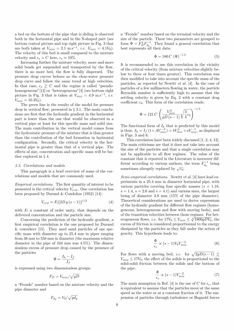
This paragraph is devoted to the comparison of thepressure drop curves with various concentrations, specificmasses and sizes for identical spherical beads. The ref-erence case is the Alumina beads of diameter 6 mm, ofspecific mass s = 3.65, and at a delivered concentrationC = 5%. In this case, the order of magnitude of the min-imal pressure drop at critical velocity Vcrit, h ' 2.4 m.s−1

is Icrit, h ' 0.11 m/m.The effects of the concentration are presented in Fig. 4a-

b. Only results for the horizontal part are plotted. On the

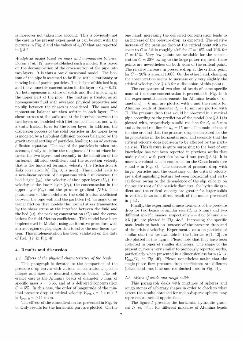
one hand, increasing the delivered concentration leads toan increase of the pressure drop, as expected. The relativeincrease of the pressure drop at the critical point with re-spect to C = 5% is roughly 40% for C = 10% and 70% forC = 15%. Very few points are available for the concen-tration C = 20% owing to the large power required; thesepoints are nevertheless on both sides of the critical point.The relative increase in pressure drop at the critical pointfor C = 20% is around 100%. On the other hand, changingthe concentration seems to increase only very slightly thecritical velocity (see § 4.3 for a discussion of this point).

The comparison of two sizes of beads of same specificmass at the same concentration is presented in Fig. 4c-d:the experimental measurements for Alumina beads of di-ameter dp = 6 mm are plotted with ◦ and the results forAlumina beads of diameter dp = 15 mm are plotted with�. The pressure drop that would be observed in a verticalpipe according to the prediction of the model (see § 3.1) isplotted with, respectively a solid red line for dp = 6 mmand a dashed red line for dp = 15 mm. The main effects ofthe size are first that the pressure drop is decreased for thelarge particles in the horizontal pipe, and secondly that thecritical velocity does not seem to be affected by the parti-cle size. This feature is quite surprising to the best of ourknowledge has not been reported in previous works thatmainly dealt with particles below 4 mm (see § 3.3). It ismoreover robust as it is confirmed on the Glass beads (see? and � in Fig. 8). The decrease of pressure drop withlarger particles and the constancy of the critical velocityare a distinguishing feature between horizontal and verti-cal flows: owing to the dependence of the slip velocity onthe square root of the particle diameter, the hydraulic gra-dient and the critical velocity are greater for larger solidsin vertical flows as a direct result of the model presentedin § 3.1.

Finally, the experimental measurements of the pressuredrop for two beads of similar size (dp ' 5 mm) and twodifferent specific masses, respectively s = 3.65 (◦) and s =2.5 (F) are plotted in Fig. 4e-f. Increasing the specificmass leads to both an increase of the pressure drop andof the critical velocity. Experimental data on particles ofsimilar size that are available in the Literature [4, 12] arealso plotted in this figure. Please note that they have beencollected in pipes of smaller diameters. The shape of thepresent curves is very similar to previously reported works,particularly when presented in a dimensionless form (λ vs.Vmix/V0, in Fig. 4f). Please nonetheless notice that thesingle-phase flow pressure drop coefficients are different(black solid line, blue and red dashed lines in Fig. 4f).

4.2. Mixes of beads and rough solids

This paragraph deals with mixtures of spheres andrough stones of arbitrary shapes in order to check to whatextent the results obtained for mono-disperse spheres mayrepresent an actual application.

The figure 5 presents the horizontal hydraulic gradi-ent Ih vs. Vmix for different mixtures of Alumina beads

7

10−2

10−1

100

λ

(b)

10−2

10−1

100

λ(d)

0 1 2 3 4 5 6 7 8 9 1010

−2

10−1

100

Vmix

/V0

λ

(f)

0

0.05

0.1

0.15

0.2

0.25

I (m

/m)

(a)

0

0.1

0.2

0.3

0.4

0.5

I (m

/m)

(c)

0 1 2 3 4 50

0.05

0.1

0.15

0.2

0.25

0.3

0.35

0.4

Vmix

(m.s−1

)

I(m

/m)

(e)

Figure 4: (a,c,e): Hydraulic gradient Ih vs. mixture velocity Vmix. (b,d,f): dimensionless plot of λh vs. Vmix/V0.(a-b): Experimental data for Alumina beads of dp = 6 mm at various concentrations: C = 5% (◦), C = 10% (5), C = 15% (/) and C = 20%(+). Solid black line: water flowing alone.(c-d): Experimental data in the horizontal pipe (symbols) and predictions of the model presented in § 3.1 for a similar vertical pipe (redlines), for Alumina beads at C = 5% and two sizes: dp = 6 mm (◦ and solid red line) and dp = 15 mm (� and dashed red line).(e-f): Experimental data for dp = 5&6 mm and C = 5% for two specific masses: Alumina (◦) and Glass (F). Blue �: data extracted fromFig. 3 of Ref. [12] (particles of diameter dp = 3 mm, s = 1.24 flowing in an horizontal pipe of diameter D = 50 mm at C = 4.2%), solid blueline: validation of the two-layer model, dashed blue line: single phase pressure drop. Red ×: data extracted from Fig. 12 of Ref. [4] (gravelsof mean diameter dp = 3.8 mm, s = 2.55 flowing in an horizontal pipe of diameter D = 25.4 mm at C = 5%), red dashed line: single phasepressure drop.

8

0 2 4 6 8 1010

−2

10−1

100

Vmix

/V0

λ

(b)

0 0.5 1 1.5 2 2.5 3 3.5 4 4.5 50

0.05

0.1

0.15

0.2

0.25

Vmix

(m.s−1

)

I (m

/m)

(a)

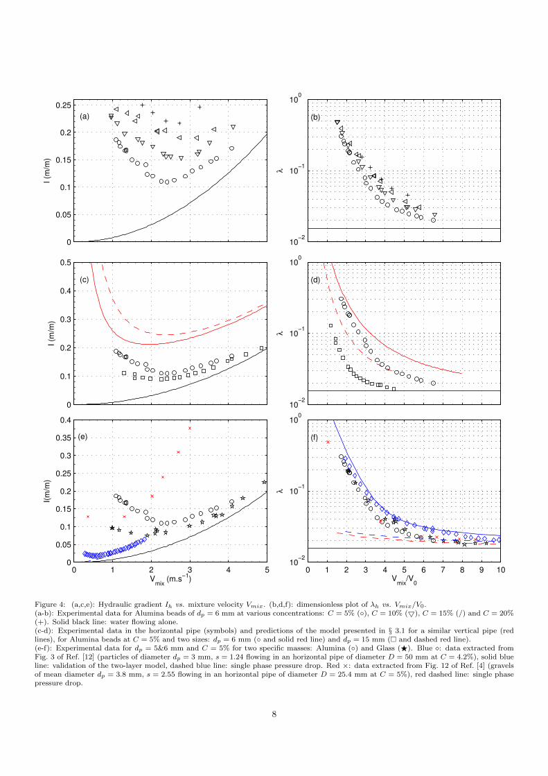
Figure 5: (a): Hydraulic gradient Ih vs. mixture velocity Vmix

and (b): dimensionless plot of λh vs. Vmix/V0, at C = 5% vs. for ◦:Alumina 6 mm, �: Alumina 15 mm,4: mixture 1 andF: mixture 2.

of diameter 6 mm and 15 mm. Contrary to what onemight think a priori, the pressure drop of the mixturesis not a simple linear combination of the pressure drop ofeach bead size: for a 50% of 6 mm mixture (mixture 1)the pressure drop curve coincides with that of the 15 mmbeads. The pressure drop is thus low. This effect is evenstill present for a proportion of 75% of 6 mm beads inthe mixture (mixture 2) but only at low mixture veloci-ties corresponding to Vmix . Vcrit, i.e. to regimes with astationary bed. For higher velocities the pressure drop liesbetween the other two and is closer to the pressure dropof the 6 mm beads.

The figure 6 presents the comparison of Ih (Vmix) forthree mixtures of beads of same size but different specificmass: Glass beads of 5 mm (F), Alumina beads of 6 mm(◦) and mixture 3 (50% Glass / 50% Alumina, /). Thepressure drop curve for the mixture lies between the twosingle-type cases and seems to be well modelized by themean of the two curves: the solid red line in Fig. 6 is a fitfor the Alumina, the solid blue line a fit for Glass and theblack line is the mean of these two curves.

0 2 4 6 8 1010

−2

10−1

100

Vmix

/V0

λ

(b)

0 0.5 1 1.5 2 2.5 3 3.5 4 4.5 50

0.05

0.1

0.15

0.2

0.25

Vmix

(m.s−1

)

I (m

/m)

(a)

Figure 6: (a): Hydraulic gradient Ih vs. mixture velocity Vmix and(b): dimensionless plot of λh vs. Vmix/V0, at C = 5% for ◦: Alumina6 mm with a fit corresponding to the red line, F: Glass 5 mm with afit corresponding to the blue line and /: mixture 3. The black solidline is the mean of the two fits.

Figure 7: Illustration of segregation for mixture 2. In that case,C = 5% and Vmix ' 1m.s−1.

9

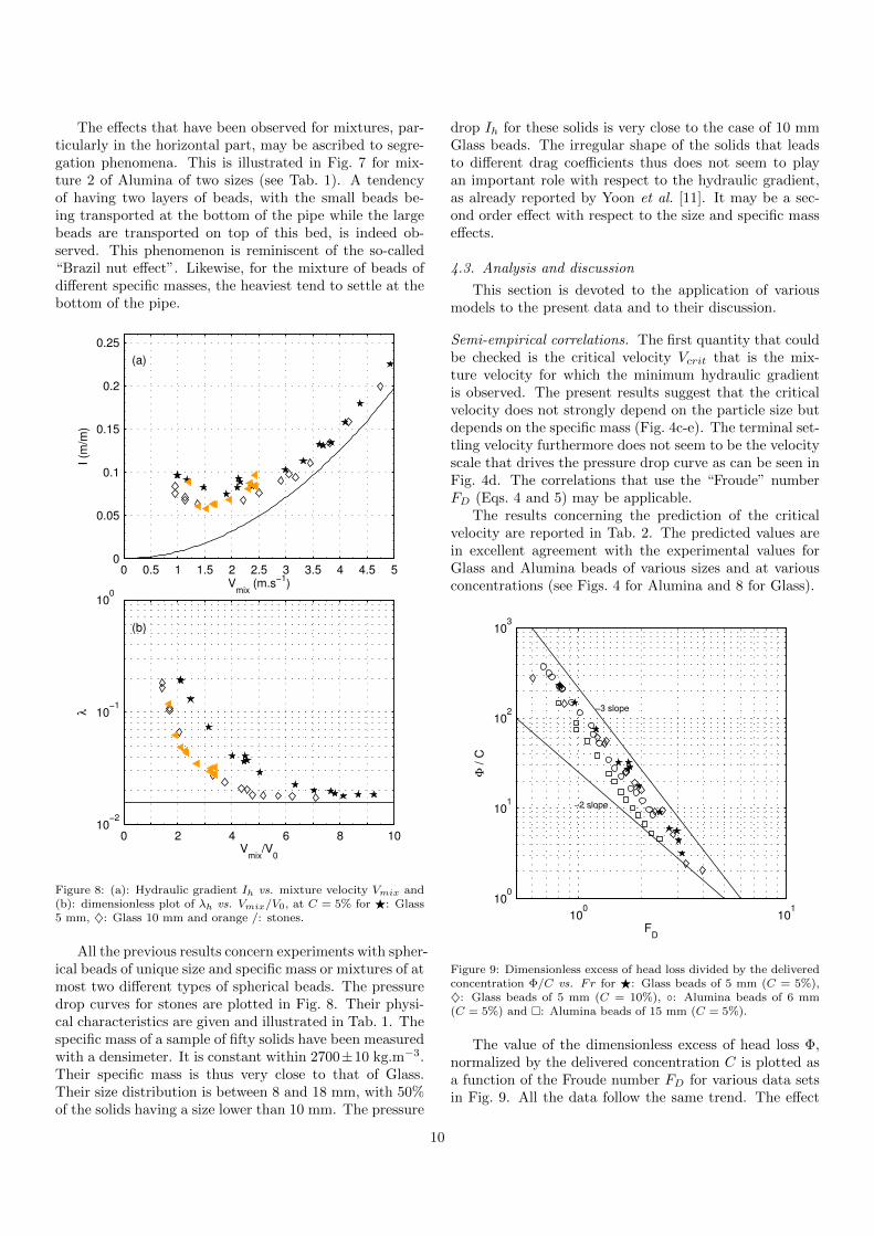
The effects that have been observed for mixtures, par-ticularly in the horizontal part, may be ascribed to segre-gation phenomena. This is illustrated in Fig. 7 for mix-ture 2 of Alumina of two sizes (see Tab. 1). A tendencyof having two layers of beads, with the small beads be-ing transported at the bottom of the pipe while the largebeads are transported on top of this bed, is indeed ob-served. This phenomenon is reminiscent of the so-called“Brazil nut effect”. Likewise, for the mixture of beads ofdifferent specific masses, the heaviest tend to settle at thebottom of the pipe.

0 2 4 6 8 1010

−2

10−1

100

Vmix

/V0

λ

(b)

0 0.5 1 1.5 2 2.5 3 3.5 4 4.5 50

0.05

0.1

0.15

0.2

0.25

Vmix

(m.s−1

)

I (m

/m)

(a)

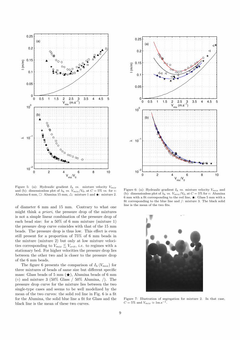
Figure 8: (a): Hydraulic gradient Ih vs. mixture velocity Vmix and(b): dimensionless plot of λh vs. Vmix/V0, at C = 5% for F: Glass5 mm, ♦: Glass 10 mm and orange /: stones.

All the previous results concern experiments with spher-ical beads of unique size and specific mass or mixtures of atmost two different types of spherical beads. The pressuredrop curves for stones are plotted in Fig. 8. Their physi-cal characteristics are given and illustrated in Tab. 1. Thespecific mass of a sample of fifty solids have been measuredwith a densimeter. It is constant within 2700±10 kg.m−3.Their specific mass is thus very close to that of Glass.Their size distribution is between 8 and 18 mm, with 50%of the solids having a size lower than 10 mm. The pressure

drop Ih for these solids is very close to the case of 10 mmGlass beads. The irregular shape of the solids that leadsto different drag coefficients thus does not seem to playan important role with respect to the hydraulic gradient,as already reported by Yoon et al. [11]. It may be a sec-ond order effect with respect to the size and specific masseffects.

4.3. Analysis and discussion

This section is devoted to the application of variousmodels to the present data and to their discussion.

Semi-empirical correlations. The first quantity that couldbe checked is the critical velocity Vcrit that is the mix-ture velocity for which the minimum hydraulic gradientis observed. The present results suggest that the criticalvelocity does not strongly depend on the particle size butdepends on the specific mass (Fig. 4c-e). The terminal set-tling velocity furthermore does not seem to be the velocityscale that drives the pressure drop curve as can be seen inFig. 4d. The correlations that use the “Froude” numberFD (Eqs. 4 and 5) may be applicable.

The results concerning the prediction of the criticalvelocity are reported in Tab. 2. The predicted values arein excellent agreement with the experimental values forGlass and Alumina beads of various sizes and at variousconcentrations (see Figs. 4 for Alumina and 8 for Glass).

100

101

100

101

102

103

FD

Φ /

C

−3 slope

−2 slope

Figure 9: Dimensionless excess of head loss divided by the deliveredconcentration Φ/C vs. Fr for F: Glass beads of 5 mm (C = 5%),♦: Glass beads of 5 mm (C = 10%), ◦: Alumina beads of 6 mm(C = 5%) and �: Alumina beads of 15 mm (C = 5%).

The value of the dimensionless excess of head loss Φ,normalized by the delivered concentration C is plotted asa function of the Froude number FD for various data setsin Fig. 9. All the data follow the same trend. The effect

10

Glass 5 mm, C = 5% Alumina 6 mm, C = 5%Experiment 1.8 2.4

Eq. 4 with Fl = 1 1.7 2.3Eq. 4 with Fl = 1.05 1.8 2.4

Table 2: Critical velocity Vcrit (m.s−1) experimentally measured for Alumina and Glass beads, compared to the values predicted with thecorrelation 4.

of the concentration is moreover well described by a lin-ear dependence: the data points for Glass beads of 5 mmat a concentration C = 5% (F) and at a concentrationC = 10% (♦) collapse on a single curve. A −3 powerlaw Φ = C K F−3

D fits quite well the data in the range0.7 . FD . 3. The effect of specific mass that is includedin the definition of the Froude number seems to be welltaken into account: the data points for Glass beads of5 mm at a concentration C = 5%, C = 10% (F & ♦) andfor Alumina beads of 6 mm at a concentration C = 5% (◦)are very close, the values of the constant K being respec-tively 130 ± 4 and 123 ± 3. All these considerations areconsistent with the empirical correlation (Eq. 5) and thetheoretical equation (Eq. 6) with V0 ∝

√s− 1 for large

particles. On the contrary, the −2 power law and the de-pendency in (s− 1) of Φ that are predicted by Eq. 7 doesnot seem to be consistent with the present measurements.As already noticed, the size of the particles, that is nottaken into account in the model, has a strong influenceon the hydraulic gradient: the value of the constant forGlass beads of 10 mm (not represented in Fig. 9) is indeedK = 87 and the value for Alumina beads of 15 mm (�) isK = 75. This is predicted neither by Eq. 5 (no dependencein dp) nore by Eq. 6 (Φ increases as

√dp). The model

that leads to Eqs. 6 and 7 relies on the hypothesis thatεs ∝ C. This is not the case in the present experiements:for Glass beads of dp = 5 mm at C = 5%, the valuesof the in situ concentration estimated with imaging areindeed: εs ' 32%, 10% and 7% for Vmix/Vcrit,h = 0.67,1.17 and 2.72. For the Alumina beads of dp = 6 mm anddp = 15 mm, the measured concentrations are εs ' 11%and 9% for Vmix/Vcrit,h = 0.83 and 1.66.

Analytical model based on mass and momentum balance.The question that is adressed is to what extent the ana-lytical model of Doron et al. [12] may apply to the presentphysical parameters, with solids of much higher specificmass and even higher relative diameter.

In the original work of Doron et al. [12], the values ofthe parameters are the following: η = 0.3, tanϕ = 0.6 andCb = 0.52. The packing concentration Cb has first beenexperimentally measured by weighting a tube of same di-ameter and capacity two liters filled with dry beads andwith beads and water. A dozen of measurements havebeen performed for each type of bead. The concentra-tion is found to be 0.52 ± 0.01. The determination of thesolid friction coefficient for an immersed granular bed isa very difficult problem [18], and the friction coefficient

0 0.5 1 1.5 2 2.5 3 3.5 4 4.5 50

0.05

0.1

0.15

0.2

0.25

Vmix

(m.s−1

)

I (m

/m)

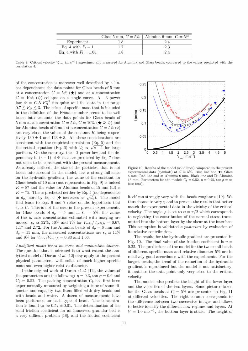
Figure 10: Results of the model (solid lines) compared to the presentexperimental data (symbols) at C = 5%. Blue line and F: Glass5 mm. Red line and ◦: Alumina 6 mm. Black line and �: Alumina15 mm. Parameters for the model: Cb = 0.52, η = 0.25, tanϕ = ∞(see text).

itself can strongly vary with the beads roughness [19]. Wethus choose to vary η and to present the results that bettermatch the experimental data in the vicinity of the criticalvelocity. The angle ϕ is set to ϕ = π/2 which correspondsto neglecting the contribution of the normal stress trans-mitted into the bottom layer by the shear at the interface.This asumption is validated a posteriori by evaluation ofits relative contribution.

The results for the hydraulic gradient are presented inFig. 10. The final value of the friction coefficient is η =0.25. The predictions of the model for the two small beadsof different specific mass and relative diameter 5% are inrelatively good accordance with the experiments. For thelargest beads, the trend of the reduction of the hydraulicgradient is reproduced but the model is not satisfactory:it matches the data point only very close to the criticalvelocity.

The models also predicts the height of the lower layerand the velocities of the two layers. Some pictures takenfor the Glass beads at C = 5% are presented in Fig. 11at different velocities. The right column corresponds tothe difference between two successive images and allowsto better identify the different flow regimes and layers. AtV = 1.0 m.s−1, the bottom layer is static. The height of

11

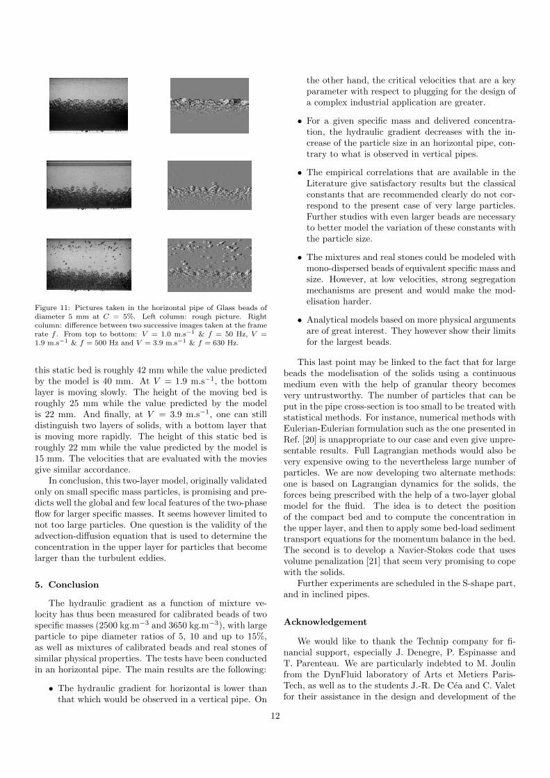
Figure 11: Pictures taken in the horizontal pipe of Glass beads ofdiameter 5 mm at C = 5%. Left column: rough picture. Rightcolumn: difference between two successive images taken at the framerate f . From top to bottom: V = 1.0 m.s−1 & f = 50 Hz, V =1.9 m.s−1 & f = 500 Hz and V = 3.9 m.s−1 & f = 630 Hz.

this static bed is roughly 42 mm while the value predictedby the model is 40 mm. At V = 1.9 m.s−1, the bottomlayer is moving slowly. The height of the moving bed isroughly 25 mm while the value predicted by the modelis 22 mm. And finally, at V = 3.9 m.s−1, one can stilldistinguish two layers of solids, with a bottom layer thatis moving more rapidly. The height of this static bed isroughly 22 mm while the value predicted by the model is15 mm. The velocities that are evaluated with the moviesgive similar accordance.

In conclusion, this two-layer model, originally validatedonly on small specific mass particles, is promising and pre-dicts well the global and few local features of the two-phaseflow for larger specific masses. It seems however limited tonot too large particles. One question is the validity of theadvection-diffusion equation that is used to determine theconcentration in the upper layer for particles that becomelarger than the turbulent eddies.

5. Conclusion

The hydraulic gradient as a function of mixture ve-locity has thus been measured for calibrated beads of twospecific masses (2500 kg.m−3 and 3650 kg.m−3), with largeparticle to pipe diameter ratios of 5, 10 and up to 15%,as well as mixtures of calibrated beads and real stones ofsimilar physical properties. The tests have been conductedin an horizontal pipe. The main results are the following:

• The hydraulic gradient for horizontal is lower thanthat which would be observed in a vertical pipe. On

the other hand, the critical velocities that are a keyparameter with respect to plugging for the design ofa complex industrial application are greater.

• For a given specific mass and delivered concentra-tion, the hydraulic gradient decreases with the in-crease of the particle size in an horizontal pipe, con-trary to what is observed in vertical pipes.

• The empirical correlations that are available in theLiterature give satisfactory results but the classicalconstants that are recommended clearly do not cor-respond to the present case of very large particles.Further studies with even larger beads are necessaryto better model the variation of these constants withthe particle size.

• The mixtures and real stones could be modeled withmono-dispersed beads of equivalent specific mass andsize. However, at low velocities, strong segregationmechanisms are present and would make the mod-elisation harder.

• Analytical models based on more physical argumentsare of great interest. They however show their limitsfor the largest beads.

This last point may be linked to the fact that for largebeads the modelisation of the solids using a continuousmedium even with the help of granular theory becomesvery untrustworthy. The number of particles that can beput in the pipe cross-section is too small to be treated withstatistical methods. For instance, numerical methods withEulerian-Eulerian formulation such as the one presented inRef. [20] is unappropriate to our case and even give unpre-sentable results. Full Lagrangian methods would also bevery expensive owing to the nevertheless large number ofparticles. We are now developing two alternate methods:one is based on Lagrangian dynamics for the solids, theforces being prescribed with the help of a two-layer globalmodel for the fluid. The idea is to detect the positionof the compact bed and to compute the concentration inthe upper layer, and then to apply some bed-load sedimenttransport equations for the momentum balance in the bed.The second is to develop a Navier-Stokes code that usesvolume penalization [21] that seem very promising to copewith the solids.

Further experiments are scheduled in the S-shape part,and in inclined pipes.

Acknowledgement

We would like to thank the Technip company for fi-nancial support, especially J. Denegre, P. Espinasse andT. Parenteau. We are particularly indebted to M. Joulinfrom the DynFluid laboratory of Arts et Metiers Paris-Tech, as well as to the students J.-R. De Cea and C. Valetfor their assistance in the design and development of the

12

experiment. The main part of the experiments have beencarried out with the help of A. Lemaire.

[1] P.E. Baha Abulnaga. Slurry Systems Handbook. McGraw-Hill,2002.

[2] K. C. Wilson, G. R. Addie, A. Sellgren, and R. Clift. SlurryTransport Using Centrifugal Pumps. Springer, 2006.

[3] V. Matousek. Predictive model for frictional pressure drop insettling-slurry pipe with stationary deposit. Powder Technol-ogy, 192:367–374, 2009.

[4] D. M. Newitt, J. F. Richardson, M. Abbott, and R. B. Turtle.Hydraulic conveying of solids in horizontal pipes. Trans. Instn.Chem. Engrs., 33:93–110, 1955.

[5] H. E. Engelmann. Vertical hydraulic lifting of large-size particles— a contribution to marine mining. In 10th Off. Tech. Conf.,pages 731–740, 1978.

[6] K. Pougatch and M. Salcudean. Numerical modeling of deepsea air-lift. Ocean Engineering, 35:1173, 2008.

[7] D. M. Newitt, J. F. Richardson, and B. J. Gliddon. Hydraulicconveying of solids in vertical pipes. Trans. Instn. Chem. En-grs., 39:93–100, 1961.

[8] J. F. Richardson and W. N. Zaki. Sedimentation and fluidisa-tion. Trans. Inst. Chem. Engrs., 32:35–53, 1957.

[9] J. X. Xia, J. R. Ni, and C. Mendoza. Hydraulic lifting of man-ganese nodules through a riser. J. Offshore Mechanics and Arc-tic Engineering, 126:72, 2004.

[10] S. Hong, J. Choi, and C. K. Yang. Experimental study onsolid-water slurry flow in vertical pipe by using ptv method. InProceedings of the Twelfth (2002) International Offshore andPolar Engineering Conference, pages 462–466, 2002.

[11] C. H. Yoon, J. S. Kang, Y. C. Park, Y. J. Kim, J. M. Park, andS. K. Kwon. Solid-liquid flow experiment with real and artifi-cial manganese nodules in flexible hoses. In Proceedings of theEighteenth (2008) International Offshore and Polar Engineer-ing Conference, pages 68–72, 2008.

[12] P. Doron, D. Granica, and D. Barnea. Slurry flow in horizontalpipes - experimental and modeling. Int. J. Multiphase Flow,13:535–547, 1987.

[13] P. Doron, M. Simkhis, and D. Barnea. Flow of solid-liquidmixtures in inclined pipes. Int. J. Multiphase Flow, 23:313–323, 1997.

[14] R. Durand and E. Condolios. Experimental investigation ofthe transport of solids in pipes. In Deuxieme Journee de lhy-draulique, Societe Hydrotechnique de France, 1952.

[15] R. Durand. Basic relationship of the transportation of solidsin pipes—experimental research. In Proc. Minnesota Interna-tional Hydraulics Conference, pages 89–103, 1953.

[16] V. Matousek. Pressure drops and flow patterns in sand-mixturepipes. Experimental thermal and fluid science, 26:693–702,2002.

[17] H. Yamaguchi, X.-D. Niu, S. Nagaoka, and F. de Vuyst. Solid-liquid two-phase flow measurement using an electromagneti-cally induced signal measurement method. J. Fluids Eng.,133:041302, 2011.

[18] T. Divoux and J.-C. Geminard. Friction and dilatancy in im-mersed granular matter. Physical review letters, 99:258301,2007.

[19] N. A. Pohlman, B. L. Severson, J. M. Ottino, and R. M. Luep-tow. Surface roughness effects in granular matter: Influence onangle of repose and the absence of segregation. Physical ReviewE, 73:031304, 2006.

[20] J. Ling, P. V. Skudarnov, C. X. Lin, and M. A. Ebadian. Numer-ical investigations of liquid-solid slurry flows in a fully developedturbulent flow region. Int. J. Heat and Fluid Flow, 24:389–398,2003.

[21] D. Kolomenskiy and K. Schneider. A fourier spectral method forthe navier-stokes equations with volume penalization for movingsolid obstacles. Journal of Computational Physics, 228:5687–5709, 2009.

13