EXPERIMENTAL STUDY OF ENERGY-MINIMIZING · PDF fileEXPERIMENTAL STUDY OF ENERGY-MINIMIZING POINT CONFIGURATIONS ON SPHERES ... deﬁne the f-potential energy of a ﬁnite subset C

arX

iv:m

ath/

0611

451v

3 [

mat

h.M

G]

7 O

ct 2

008

EXPERIMENTAL STUDY OF ENERGY-MINIMIZING

POINT CONFIGURATIONS ON SPHERES

BRANDON BALLINGER, GRIGORIY BLEKHERMAN, HENRY COHN,NOAH GIANSIRACUSA, ELIZABETH KELLY, AND ACHILL SCHURMANN

Abstract. In this paper we report on massive computer experiments aimedat finding spherical point configurations that minimize potential energy. Wepresent experimental evidence for two new universal optima (consisting of 40points in 10 dimensions and 64 points in 14 dimensions), as well as evidencethat there are no others with at most 64 points. We also describe several othernew polytopes, and we present new geometrical descriptions of some of theknown universal optima.

[T]he problem of finding the configurations of stable equilibriumfor a number of equal particles acting on each other according tosome law of force. . . is of great interest in connexion with the rela-tion between the properties of an element and its atomic weight.Unfortunately the equations which determine the stability of sucha collection of particles increase so rapidly in complexity with thenumber of particles that a general mathematical investigation isscarcely possible.

J. J. Thomson, 1897

Contents

1. Introduction 21.1. Experimental results 41.2. New universal optima 82. Methodology 92.1. Techniques 92.2. Example 143. Experimental phenomena 153.1. Analysis of Gram matrices 153.2. Other small examples 183.3. 2n+ 1 points in Rn 203.4. 2n+ 2 points in Rn 213.5. 48 points in R

4 223.6. Hopf structure 233.7. Facet structure of universal optima 233.8. 96 points in R9 27

Date: September 8, 2008.Ballinger and Giansiracusa were supported by the University of Washington Mathematics

Department’s NSF VIGRE grant. Schurmann was supported by the Deutsche Forschungsgemein-schaft (DFG) under grant SCHU 1503/4-1.

1

http://arXiv.org/abs/math/0611451v3

2 BALLINGER, BLEKHERMAN, COHN, GIANSIRACUSA, KELLY, AND SCHURMANN

3.9. Distribution of energy levels 284. Conjectured universal optima 304.1. 40 points in R10 304.2. 64 points in R14 325. Balanced, irreducible harmonic optima 336. Challenges 36Acknowledgements 36Appendix A. Local non-optimality of diplo-simplices 36References 38

1. Introduction

What is the best way to distribute N points over the unit sphere Sn−1 in Rn?Of course the answer depends on the notion of “best.” One particularly interestingcase is energy minimization. Given a continuous, decreasing function f : (0, 4] → R,define the f -potential energy of a finite subset C ⊂ Sn−1 to be

Ef (C) =1

2

∑

x,y∈Cx 6=y

f(

|x− y|2)

.

(We only need f to be defined on (0, 4] because |x− y|2 ≤ 4 when |x|2 = |y|2 = 1.The factor of 1/2 is chosen for compatibility with the physics literature, whilethe use of squared distance is incompatible but more convenient.) How can onechoose C ⊂ Sn−1 with |C| = N so as to minimize Ef (C)? In this paper wereport on lengthy computer searches for configurations with low energy. Whatdistinguishes our approach from most earlier work on this topic (see for example[AP-G1, AP-G2, AP-G3, AWRTSDW, AW, BBCDHNNTW, BCNT1, BCNT2, C,DM, DLT, E, ELSBB, EH, F, GE, HSa1, HSa2, H, KaS, KuS, Ko, LL, M-FMRS,MKS, MDH, P-GDMOD-S, P-GDM, P-GM, RSZ1, RSZ2, SK, Sl, T, Wh, Wil]) isthat we attempt to treat many different potential functions on as even a footingas possible. Much of the mathematical structure of this problem becomes appar-ent only when one varies the potential function f . Specifically, we find that manyoptimal configurations vary in surprisingly simple, low-dimensional families as fvaries.

The most striking case is when such a family is a single point: in other words,when the optimum is independent of f . Cohn and Kumar [CK] defined a configu-ration to be universally optimal if it minimizes Ef for all completely monotonic f

(i.e., f is infinitely differentiable and (−1)kf (k)(x) ≥ 0 for all k ≥ 0 and x ∈ (0, 4),as is the case for inverse power laws). They were able to prove universal optimalityonly for certain very special arrangements. One of our primary goals in this paperis to investigate how common universal optimality is. Was the limited list of exam-ples in [CK] an artifact of the proof techniques or a sign that these configurationsare genuinely rare?

Every universally optimal configuration is an optimal spherical code, in the sensethat it maximizes the minimal distance between the points. (Consider an inversepower law f(r) = 1/rs. If there were a configuration with a larger minimal distance,then its f -potential energy would be lower when s is sufficiently large.) However,universal optimality is a far stronger condition than optimality as a spherical code.

ENERGY-MINIMIZING POINT CONFIGURATIONS 3

n N t Description2 N cos(2π/N) N -gonn N ≤ n+ 1 −1/(N − 1) simplexn 2n 0 cross polytope

3 12 1/√

5 icosahedron

4 120 (1 +√

5)/4 regular 600-cell5 16 1/5 hemicube/Clebsch graph6 27 1/4 Schlafli graph/isotropic subspaces7 56 1/3 equiangular lines8 240 1/2 E8 root system21 112 1/9 isotropic subspaces21 162 1/7 (162, 56, 10, 24) strongly regular graph22 100 1/11 Higman-Sims graph22 275 1/6 McLaughlin graph22 891 1/4 isotropic subspaces23 552 1/5 equiangular lines23 4600 1/3 kissing configuration of the following24 196560 1/2 Leech lattice minimal vectors

q q3+1q+1 (q + 1)(q3 + 1) 1/q2 isotropic subspaces (q is a prime power)

Table 1. The known universal optima.

There are optimal spherical codes of each size in each dimension, but they are rarelyuniversally optimal. In three dimensions, the only examples are a single point, twoantipodal points, an equilateral triangle on the equator, or the vertices of a regulartetrahedron, octahedron, or icosahedron. Universal optimality was proved in [CK],building on previous work by Yudin, Kolushov, and Andreev [Y, KY1, KY2, A1,A2], and the completeness of this list follows from a classification theorem due toLeech [L]. See [CK] for more details.

In higher dimensions much less is known. Cohn and Kumar’s main theoremprovides a general criterion from which they deduced the universal optimality of anumber of previously studied configurations. Specifically, they proved that everyspherical (2m−1)-design in which only m distances occur between distinct points isuniversally optimal. Recall that a spherical d-design in Sn−1 is a finite subset C ofSn−1 such that every polynomial on Rn of total degree d has the same average overC as over the entire sphere. This criterion holds for every known universal optimumexcept one case, namely the regular 600-cell in R4 (i.e., the H4 root system), forwhich Cohn and Kumar proved universal optimality by a special argument.

A list of all known universal optima is given in Table 1. Here n is the dimensionof the Euclidean space, N is the number of points, and t is the greatest innerproduct between distinct points in the configuration (i.e., the cosine of the minimalangle). For detailed descriptions of these configurations, see Section 1 of [CK].Each is uniquely determined by the parameters listed in Table 1, except for theconfigurations listed on the last line. For that case, when q = pℓ with p an oddprime, there are at least ⌊(ℓ−1)/2⌋ distinct universal optima (see [CGS] and [Ka]).Classifying these optima is equivalent to classifying generalized quadrangles with


n N t References10 40 1/6 Conway, Sloane, and Smith [Sl], Hovinga [H]14 64 1/7 Nordstrom and Robinson [NR], de Caen and van Dam [dCvD],

Ericson and Zinoviev [EZ]

Table 2. New conjectured universal optima.

parameters (q, q2), which is a difficult problem in combinatorics. In the other casesfrom Table 1, when uniqueness holds, we use the notation UN,n for the uniqueN -point universal optimum in R

n.Each of the configurations in Table 1 had been studied before it appeared in [CK],

and was already known to be an optimal spherical code. In fact, when N ≥ 2n+ 1and n > 4, the codes on this list are exactly those that have been proved optimal.Cohn and Kumar were unable to resolve the question of whether Table 1 is thecomplete list of universally optimal codes, except when n ≤ 3. All that is known ingeneral is that any new universal optimum must have N ≥ 2n+ 1 (Proposition 1.4in [CK]). It does not seem plausible that the current list is complete, but it is farfrom obvious where to find any others.

Each known universal optimum is a beautiful mathematical object, connected tovarious important exceptional structures (such as special lattices or groups). Ourlong-term hope is to develop automated tools that will help uncover more suchobjects. In this paper we do not discover any configurations as fundamental asthose in Table 1, but perhaps our work is a first step in that direction.

Table 1 shows several noteworthy features. When n ≤ 4, the codes listed arethe vertices of regular polytopes, specifically those with simplicial facets. When5 ≤ n ≤ 8, the table also includes certain semiregular polytopes (their facets aresimplices and cross polytopes, with two cross polytopes and one simplex arrangedaround each (n − 3)-dimensional face). The corresponding spherical codes are allaffine cross sections of the minimal vectors of the E8 root lattice. Remarkably,no universal optima are known for 9 ≤ n ≤ 20, except for the simplices and crosspolytopes, which exist in every dimension. This gap is troubling—why should thesedimensions be disfavored? For 21 ≤ n ≤ 24 nontrivial universal optima are known;they are all affine cross sections of the minimal vectors of the Leech lattice (andare no longer the vertices of semiregular polytopes). Finally, in high dimensions asingle infinite sequence of nontrivial universal optima is known.

It is not clear how to interpret this list. For example, is the dimension gap real,or merely an artifact of humanity’s limited imagination? One of our conclusions inthis paper is that Table 1 is very likely incomplete but appears closer to completethan one might expect.

1.1. Experimental results. One outcome of our computer searches is two candi-date universal optima, listed in Table 2 and described in more detail in Section 4.These configurations were located through massive computer searches: for each ofmany pairs (n,N), we repeatedly picked N random points on Sn−1 and performedgradient descent to minimize potential energy. We focused on the potential functionf(r) = 1/rn/2−1, because x 7→ 1/|x|n−2 is the unique nonconstant radial harmonicfunction on R

n \ {0}, up to scalar multiplication (recall that distance is squared


Pro

babi

lity

0

1

2 64Number of points

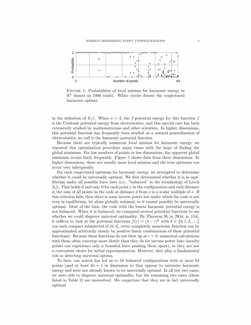
Figure 1. Probabilities of local minima for harmonic energy inR3 (based on 1000 trials). White circles denote the conjecturedharmonic optima.

in the definition of Ef ). When n = 3, the f -potential energy for this function fis the Coulomb potential energy from electrostatics, and this special case has beenextensively studied by mathematicians and other scientists. In higher dimensions,this potential function has frequently been studied as a natural generalization ofelectrostatics; we call it the harmonic potential function.

Because there are typically numerous local minima for harmonic energy, werepeated this optimization procedure many times with the hope of finding theglobal minimum. For low numbers of points in low dimensions, the apparent globalminimum occurs fairly frequently. Figure 1 shows data from three dimensions. Inhigher dimensions, there are usually more local minima and the true optimum canoccur very infrequently.

For each conjectured optimum for harmonic energy, we attempted to determinewhether it could be universally optimal. We first determined whether it is in equi-librium under all possible force laws (i.e., “balanced” in the terminology of Leech[L]). That holds if and only if for each point x in the configuration and each distanced, the sum of all points in the code at distance d from x is a scalar multiple of x. Ifthis criterion fails, then there is some inverse power law under which the code is noteven in equilibrium, let alone globally minimal, so it cannot possibly be universallyoptimal. Most of the time, the code with the lowest harmonic potential energy isnot balanced. When it is balanced, we compared several potential functions to seewhether we could disprove universal optimality. By Theorem 9b in [Wid, p. 154],it suffices to look at the potential functions f(r) = (4 − r)k with k ∈ {0, 1, 2, . . .}(on each compact subinterval of (0, 4], every completely monotonic function can beapproximated arbitrarily closely by positive linear combinations of these potentialfunctions). Because these functions do not blow up at r = 0, numerical calculationswith them often converge more slowly than they do for inverse power laws (nearbypoints can experience only a bounded force pushing them apart), so they are nota convenient choice for initial experimentation. However, they play a fundamentalrole in detecting universal optima.

To date, our search has led us to 58 balanced configurations with at most 64points (and at least 2n + 1 in dimension n) that appear to minimize harmonicenergy and were not already known to be universally optimal. In all but two cases,we were able to disprove universal optimality, but the remaining two cases (thoselisted in Table 2) are unresolved. We conjecture that they are in fact universallyoptimal.


Dim

ensi

on

32

32 Number of points 64

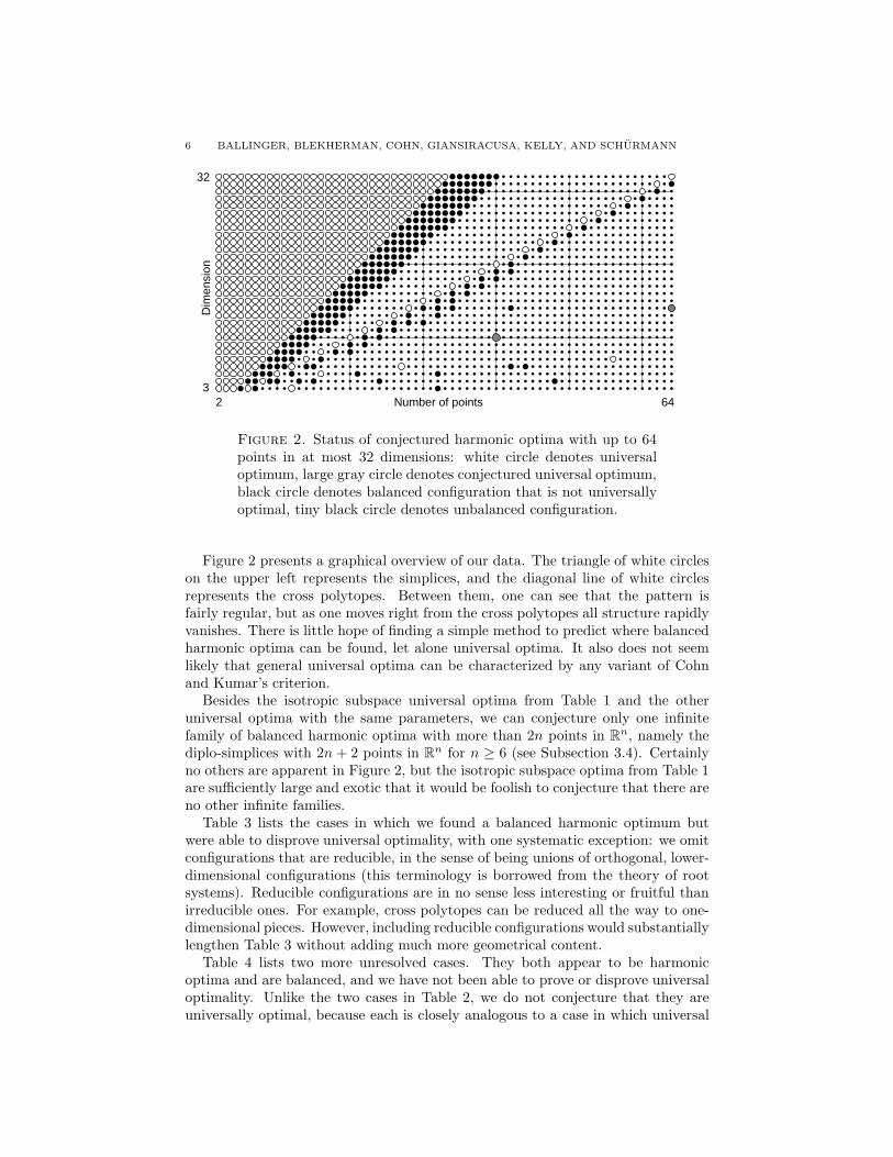
Figure 2. Status of conjectured harmonic optima with up to 64points in at most 32 dimensions: white circle denotes universaloptimum, large gray circle denotes conjectured universal optimum,black circle denotes balanced configuration that is not universallyoptimal, tiny black circle denotes unbalanced configuration.

Figure 2 presents a graphical overview of our data. The triangle of white circleson the upper left represents the simplices, and the diagonal line of white circlesrepresents the cross polytopes. Between them, one can see that the pattern isfairly regular, but as one moves right from the cross polytopes all structure rapidlyvanishes. There is little hope of finding a simple method to predict where balancedharmonic optima can be found, let alone universal optima. It also does not seemlikely that general universal optima can be characterized by any variant of Cohnand Kumar’s criterion.

Besides the isotropic subspace universal optima from Table 1 and the otheruniversal optima with the same parameters, we can conjecture only one infinitefamily of balanced harmonic optima with more than 2n points in R

n, namely thediplo-simplices with 2n+ 2 points in Rn for n ≥ 6 (see Subsection 3.4). Certainlyno others are apparent in Figure 2, but the isotropic subspace optima from Table 1are sufficiently large and exotic that it would be foolish to conjecture that there areno other infinite families.

Table 3 lists the cases in which we found a balanced harmonic optimum butwere able to disprove universal optimality, with one systematic exception: we omitconfigurations that are reducible, in the sense of being unions of orthogonal, lower-dimensional configurations (this terminology is borrowed from the theory of rootsystems). Reducible configurations are in no sense less interesting or fruitful thanirreducible ones. For example, cross polytopes can be reduced all the way to one-dimensional pieces. However, including reducible configurations would substantiallylengthen Table 3 without adding much more geometrical content.

Table 4 lists two more unresolved cases. They both appear to be harmonicoptima and are balanced, and we have not been able to prove or disprove universaloptimality. Unlike the two cases in Table 2, we do not conjecture that they areuniversally optimal, because each is closely analogous to a case in which universal


n N t

3 32√

75 + 30√

5/15

4 10 1/6 or (√

5 − 1)/44 13

(

cos(4π/13) + cos(6π/13))

/2

4 15 1/√

84 24 1/2

4 48 1/√

2

5 21 1/√

10

5 32 1/√

5n ≥ 6 2n+ 2 1/n

6 42 2/5

6 44 1/√

6

6 126√

3/87 78 3/7

7 148√

2/78 72 5/149 96 1/314 42 1/1016 256 1/4

Table 3. Conjectured harmonic optima that are balanced, irre-ducible, and not universally optimal (see Section 5 for descrip-tions).

n N t

7 182 1/√

315 128 1/5

Table 4. Unresolved conjectured harmonic optima.

optimality fails (182 points in R7 is analogous to 126 points in R6, and 128 points inR15 is analogous to 256 points in R16). On the other hand, each is also analogous toa configuration we know or believe is universally optimal (240 points in R

8 and 64points in R14, respectively). We have not been able to disprove universal optimalityin the cases in Table 4, but they are sufficiently large that our failure provides littleevidence in favor of universal optimality.

Note that the data presented in Tables 3 and 4 may not specify the configurationsuniquely. For example, for 48 points in R4 there is a positive-dimensional familyof configurations with maximal inner product 1/

√2 (which is not the best possible

value, according to Sloane’s tables [Sl]). See Section 5 for explicit constructions ofthe conjectured harmonic optima.

It is worth observing that several famous configurations do not appear in Tables 3or 4. Most notably, the cubes in Rn with n ≥ 3, the dodecahedron, the 120-cell,and the D5, E6, and E7 root systems are suboptimal for harmonic energy. Many of


these configurations have more than 64 points, but we have included in the tablesall configurations we have analyzed, regardless of size.

In each case listed in Tables 3 and 4, our computer programs returned floatingpoint approximations to the coordinates of the points in the code, but we have beenable to recognize the underlying structure exactly. That is possible largely becausethese codes are highly symmetric, and once one has uncovered the symmetries theremaining structure is greatly constrained. By contrast, for most numbers of pointsin most dimensions, we cannot even recognize the minimal harmonic energy as anexact algebraic number (although it must be algebraic, because it is definable inthe first-order theory of the real numbers).

1.2. New universal optima. Both codes listed in Table 2 have been studiedbefore. The first code was discovered by Conway, Sloane, and Smith [Sl] as aconjecture for an optimal spherical code (and discovered independently by Hovinga[H]). The second can be derived from the Nordstrom-Robinson binary code [NR]or as a spectral embedding of an association scheme discovered by de Caen and vanDam [dCvD] (take t = 1 in Theorem 2 and Proposition 7(i) in [dCvD] and thenproject the standard orthonormal basis into a common eigenspace of the operatorsin the Bose-Mesner algebra of the association scheme). We describe both codes ingreater detail in Section 4.

Neither code satisfies the condition from [CK] for universal optimality: both arespherical 3-designs (but not 4-designs), with four distances between distinct pointsin the 40-point code and three in the 64-point code. That leaves open the possibilityof an ad hoc proof, similar to the one Cohn and Kumar gave for the regular 600-cell,but the techniques from [CK] do not apply.

To test universal optimality, we have carried out 1000 random trials with thepotential function f(r) = (4 − r)k for each k from 1 to 25. We have also carriedout 1000 trials using Hardin and Sloane’s program Gosset [HSl] to construct goodspherical codes (to take care of the case when k is large). Of course these experi-mental tests fall far short of a rigorous proof, but the codes certainly appear to beuniversally optimal.

We believe that they are the only possible new universal optima consisting of atmost 64 points, because we have searched the space of such codes fairly thoroughly.By Proposition 1.4 in [CK], any new universal optimum in Rn must contain at least2n + 1 points. There are 812 such cases with at most 64 points in dimension atleast 4. In each case, we have completed at least 1000 random trials (and usuallymore). There is no guarantee that we have found the global optimum in any ofthese cases, because it could have a tiny basin of attraction. However, a simplecalculation shows that it is 99.99% likely that in every case we have found everylocal minimum that occurs at least 2% of the time. We have probably not alwaysfound the true optimum, but we believe that we have found every universal optimumwithin the range we have searched.

We have made our tables of conjectured harmonic optima for up to 64 points inup to 32 dimensions available via the world wide web at

http://aimath.org/data/paper/BBCGKS2006/.

They list the best energies we have found and the coordinates of the configurationsthat achieve them. We would be grateful for any improvements, and we intend tokeep the tables up to date, with credit for any contributions received from others.

http://aimath.org/data/paper/BBCGKS2006/


In addition to carrying out our own searches for universal optima, we have exam-ined Sloane’s tables [Sl] of the best spherical codes known with at most 130 pointsin R4 and R5, and we have verified that they contain no new universal optima.We strongly suspect that there are no undiscovered universal optima of any size inR

4 or R5, based on Sloane’s calculations as well as our searches, but it would be

difficult to give definitive experimental evidence for such an assertion (we see noconvincing arguments for why huge universal optima should not exist).

In general, our searches among larger codes have been far less exhaustive thanthose up to 64 points: we have at least briefly examined well over four thousanddifferent pairs (n,N), but generally not in sufficient depth to make a compellingcase that we have found the global minimum. (Every time we found a balancedharmonic optimum, with the exception of 128 points in R15 and 256 points in R16,we completed at least 1000 trials to test whether it was really optimal. However,we have not completed nearly as many trials in most other cases, and in any case1000 trials is not enough when studying large configurations.) Nevertheless, ourstrong impression is that universal optima are rare, and certainly that there arefew small universal optima with large basins of attraction.

2. Methodology

2.1. Techniques. As discussed in the introduction, to minimize potential energywe apply gradient descent, starting from many random initial configurations. Thatis an unsophisticated approach, because gradient descent is known to perform moreslowly in many situations than competing methods such as the conjugate gradientalgorithm. However, it has performed adequately in our computations. Further-more, gradient descent has particularly intuitive dynamics. Imagine particles im-mersed in a medium with enough viscosity that they never build up momentum.When a force acts on them according to the potential function, the configurationundergoes gradient descent. By contrast, for most other optimization methodsthe motion of the particles is more obscure, so for example it is more difficult tointerpret information such as sizes of basins of attraction.

Once one has approximate coordinates, one can use the multivariate analogueof Newton’s method to compute them to high precision (by searching for a zeroof the gradient vector). Usually we do not need to do this, because the results ofgradient descent are accurate enough for our purposes, but it is a useful tool tohave available.

Obtaining coordinates is simply the beginning of our analysis. Because thecoordinates encode not only the relative positions of the points but also an arbitraryorthogonal transformation of the configuration, interpreting the data can be subtle.A first step is to compute the Gram matrix. In other words, given points x1, . . . , xN ,compute the N×N matrix G whose entries are given by Gi,j = 〈xi, xj〉. The Grammatrix is invariant under orthogonal transformations, so it encodes almost preciselythe information we care about. Its only drawback is that it depends on the arbitrarychoice of how the points are ordered. That may sound like a mild problem, butthere are many permutations of the points and it is far from clear how to chooseone that best exhibits the configuration’s underlying structure: compare Figure 3with Figure 4.

With luck, one can recognize the entries of the Gram matrix as exact algebraicnumbers: more frequently than one might expect, they are rational or quadratic


Figure 3. The Gram matrix for a regular 600-cell (black denotes1, white denotes −1, and gray interpolates between them), withthe points ordered as returned by our gradient descent software.

Figure 4. The Gram matrix for a regular 600-cell, with the pointsordered so as to display structure.

irrationals. Once one specifies the entire Gram matrix, the configuration is com-pletely determined, up to orthogonal transformations. Furthermore, one can easilyprove that the configuration exists (keep in mind that it may not be obvious thatthere actually is such an arrangement of points, because it was arrived at via inexactcalculations). To do so, one need only check that the Gram matrix is symmetric, itis positive semidefinite, and its rank is at most n. Every such matrix is the Grammatrix of a set of N points in Rn, and if the diagonal entries are all 1 then thepoints lie on Sn−1.


Figure 5. An orthogonal projection of the conjectured harmonicoptimum with 44 points in R3 onto a random plane. Line segmentsconnect points at the minimal distance.

Figure 6. An orthogonal projection of the conjectured harmonicoptimum with 48 points in R4 onto a random plane. Line segmentsconnect points at the minimal distance.

Unfortunately, the exact Gram matrix entries are not always apparent fromthe numerical data. There is also a deeper reason why simply recognizing theGram matrix is unsatisfying: it provides only the most “bare bones” descriptionof the configuration. Many properties, such as symmetry or connections to other


mathematical structures, are far from apparent given only the Gram matrix, as onecan see from Figures 3 and 4.

Choosing the right method to visualize the data can make the underlying pat-terns clearer. For example, projections onto low-dimensional subspaces are oftenilluminating. Determining the most revealing projection can itself be difficult, butsometimes even a random projection sheds light on the structure. For example,Figures 5 and 6 are projections of the harmonic optima with 44 points in R3 and 48points in R4, respectively, onto random planes. The circular outline is the boundaryof the projection of the sphere, and the line segments pair up points separated bythe minimal distance. Figure 5 shows a disassembled cube (in a manner describedlater in this section), while Figure 6 is made up of octagons (see Subsection 3.5 fora description).

The next step in the analysis is the computation of the automorphism group.In general that is a difficult task, but we can make use of the wonderful softwareNauty written by McKay [M]. Nauty can compute the automorphism group of agraph as a permutation group on the set of vertices; more generally, it can computethe automorphism group of a vertex-labeled graph. We make use of it as follows.

Define a combinatorial automorphism of a configuration to be a permutation ofthe points that preserves inner products (equivalently, distances). If one forms anedge-labeled graph by placing an edge between each pair of points, labeled by theirinner product, then the combinatorial automorphism group is the automorphismgroup of this labeled graph. Nauty is not directly capable of computing such agroup, but it is straightforward to reduce the problem to that of computing theautomorphism group of a related vertex-labeled graph. Thus, one can use Nautyto compute the combinatorial automorphism group.

Fortunately, combinatorial automorphisms are the same as geometric symme-tries, provided the configuration spans Rn. Specifically, every combinatorial au-tomorphism is induced by a unique orthogonal transformation of Rn. (When thepoints do not span Rn, the orthogonal transformations are not unique, becausethere are nontrivial orthogonal transformations that fix the subspace spanned bythe configuration.) Thus, Nauty provides an efficient method for computing thesymmetry group.

Unfortunately, it is difficult to be certain that one has computed the correctgroup. Two inner products that appear equal numerically may differ by a tinyamount, in which case the computed symmetry group may be too large. However,that is rarely a problem even with single-precision floating point arithmetic, and itis difficult to imagine a fake symmetry that appears real to one hundred decimalplaces.

Once the symmetry group has been obtained, many further questions naturallypresent themselves. Can one recognize the symmetry group as a familiar group?How does its representation on Rn break up into irreducibles? What are the orbitsof its action on the configuration?

Analyzing the symmetries of the configuration frequently determines much of thestructure, but usually not all of it. For example, consider the simplest nontrivialcase, namely five points on S2. There are two natural ways to arrange them:with two antipodal points and three points forming an equilateral triangle on theorthogonal plane between them, or as a pyramid with four points forming a squarein the hemisphere opposite a single point (and equidistant from it). In the first


case everything is determined by the symmetries, but in the second there is onefree parameter, namely how far the square is from the point opposite it. As onevaries the potential function, the energy-minimizing value of this parameter willvary. (We conjecture that for every completely monotonic potential function, oneof the configurations described in this paragraph globally minimizes the energy, butwe cannot prove it.)

We define the parameter count of a configuration to be the dimension of the spaceof nearby configurations that can be obtained from it by applying an arbitrary radialforce law between all pairs of particles. For example, balanced configurations arethose with zero parameters, and the family with a square opposite a point has oneparameter.

To compute the parameter count for an N -point configuration, start by viewingit as an element of (Sn−1)N (by ordering the points). Within the tangent space ofthis manifold, for each radial force law there is a tangent vector. To form a basisfor all these force vectors, look at all distances d that occur in the configuration,and for each of them consider the tangent vector that pushes each pair of pointsat distance d in opposite directions but has no other effects. All force vectors arelinear combinations of these ones, and the dimension of the space they span is theparameter count for the configuration. (One must be careful to use sufficientlyhigh-precision arithmetic, as when computing the symmetry group.)

This information is useful because in a sense it shows how much humanly un-derstandable structure we can expect to find. For example, in the five-point con-figuration with a square opposite a point, the distance between them will typicallybe some complicated number depending on the potential function. In principle onecan describe it exactly, but in practice it is most pleasant to treat it as a black boxand describe all the other distances in the configuration in terms of it. The param-eter count tells how many independent parameters one should expect to arrive at.When the count is zero or one, it is reasonable to search for an elegant description,whereas when the count is twenty, it is likely that the configuration is unavoidablycomplex.

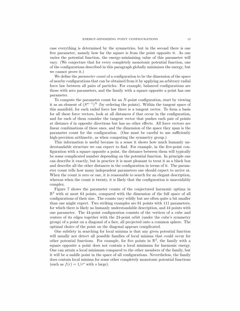
Figure 7 shows the parameter counts of the conjectured harmonic optima inR

3 with at most 64 points, compared with the dimension of the full space of allconfigurations of their size. The counts vary wildly but are often quite a bit smallerthan one might expect. Two striking examples are 61 points with 111 parameters,for which there is likely no humanly understandable description, and 44 points withone parameter. The 44-point configuration consists of the vertices of a cube andcenters of its edges together with the 24-point orbit (under the cube’s symmetrygroup) of a point on a diagonal of a face, all projected onto a common sphere. Theoptimal choice of the point on the diagonal appears complicated.

One subtlety in searching for local minima is that any given potential functionwill usually not detect all possible families of local minima that could occur forother potential functions. For example, for five points in R3, the family with asquare opposite a point does not contain a local minimum for harmonic energy.One can attain a local minimum compared to the other members of the family, butit will be a saddle point in the space of all configurations. Nevertheless, the familydoes contain local minima for some other completely monotonic potential functions(such as f(r) = 1/rs with s large).


Par

amet

er c

ount

0

130

2 64Number of points

Figure 7. Parameter counts for conjectured harmonic optima inR3. Horizontal or vertical lines occur at multiples of ten, and whitecircles denote the dimension of the configuration space.

Harmonic energy Frequency Parameters Maximal cosine Symmetries111.0000000000 99971504 0 0.2500000000 51840112.6145815185 653 9 0.4306480635 120112.6420995468 22993 18 0.3789599707 24112.7360209988 10 2 0.4015602076 1920112.8896851626 4840 13 0.4041651631 48

Table 5. Local minima for 27 points in R6 (with frequencies outof 108 random trials).

2.2. Example. For a concrete example, consider Table 5, which shows the resultsof 108 random trials for 27 points in R6 (all decimal numbers in tables have beenrounded). These parameters were chosen because, as shown in [CK], there is aunique 27-point universal optimum in R6, with harmonic energy 111; it is calledthe Schlafli configuration. The column labeled “frequency” tells how many timeseach local minimum occurred. As one can see, the universal optimum occurredmore than 99.97% of the time, but we found a total of four others.

Strictly speaking, we have not proved that the local minima listed in Table 5(other than the Schlafli configuration) even exist. They surely do, because we havecomputed them to five hundred decimal places and checked that they are localminima by numerically diagonalizing the Hessian matrix of the energy functionon the space of configurations. However, we used high-precision floating pointarithmetic, so this calculation does not constitute a rigorous proof, although itleaves no reasonable doubt. It is not at all clear whether there are additional local


Figure 8. The Clebsch graph.

minima. We have not found any, but the fact that one of the local minima occursonly once in every ten million trials suggests that there might be others with evensmaller basins of attraction.

The local minimum with energy 112.736 . . . stands out in two respects besidesits extreme rarity: it has many symmetries and it depends on few parameters.That suggests that it should have a simple description, and in fact it does, as amodification of the universal optimum. Only two inner products occur betweendistinct points in the Schlafli configuration, namely −1/2 and 1/4. In particular, itis not antipodal, so one can define a new code by replacing a single point x with itsantipode −x. The remaining 26 points can be divided into two clusters accordingto their distances from −x. Immediately after replacing x with −x the code will nolonger be a local minimum, but if one allows it to equilibrate a minimum is achieved.(That is not obvious: the code could equilibrate to a saddle point, because it isstarting from an unusual position.) All that changes is the distances of the twoclusters from −x, while the relative positions within the clusters remain unchanged(aside from rescaling). These two distances are the two parameters of the code.The symmetries of the new code are exactly those of the universal optimum thatfix x, so the size of the symmetry group is reduced by a factor of 27.

The Schlafli configuration in R6 corresponds to the 27 lines on a smooth cubicsurface: there is a natural correspondence between points in the configuration andlines on a cubic surface so that the inner products of −1/2 occur between pointscorresponding to intersecting lines. (This dates back to Schoutte [Sch]. See also theintroduction to [CK] for a brief summary of the correspondence.) One way to viewthe other local minima in Table 5 is as competitors to this classical configuration.It would be intriguing if they also had interpretations or consequences in algebraicgeometry, but we do not know of any.

3. Experimental phenomena

3.1. Analysis of Gram matrices. For an example of how one might analyze aGram matrix, consider the case of sixteen points in R5. This case also has a univer-sal optimum, in fact the smallest known one that is not a regular polytope (althoughit is semiregular). It is the five-dimensional hemicube, which consists of half the


1 a a a a a a b b b b b b b b b

a 1 e e a2 a2 a2 d c c c c d c d ca e 1 e a2 a2 a2 c d c d c c c c da e e 1 a2 a2 a2 c c d c d c d c ca a2 a2 a2 1 e e d c c c d c c c da a2 a2 a2 e 1 e c d c c c d d c ca a2 a2 a2 e e 1 c c d d c c c d c

b d c c d c c 1 f f f g g f g gb c d c c d c f 1 f g f g g f gb c c d c c d f f 1 g g f g g fb c d c c c d f g g 1 f f f g gb c c d d c c g f g f 1 f g f gb d c c c d c g g f f f 1 g g fb c c d c d c f g g f g g 1 f fb d c c c c d g f g g f g f 1 fb c d c d c c g g f g g f f f 1

Table 6. Gram matrix for 16 points in R5; here c = ab +(1/2)

√

(1 − a2)(1 − b2)/2, d = ab −√

(1 − a2)(1 − b2)/2, e =(3a2 − 1)/2, f = (3b2 − 1)/2, and g = (3b2 + 1)/4.

vertices of the cube. More precisely, it contains the points (±1,±1,±1,±1,±1)/√

5with an even number of minus signs. One can recover the full cube by includingthe antipode of each point, so the symmetries of the five-dimensional hemicubeconsist of half of those of the five-dimensional cube (namely, those that preservethe hemicube, rather than exchanging it with its complementary hemicube).

It is essentially an accident of five dimensions that the hemicube is universallyoptimal. Universal optimality also holds in lower dimensions, but only because thehemicubes turn out to be familiar codes (two antipodal points in two dimensions,a tetrahedron in three dimensions, and a cross polytope in four dimensions). Insix dimensions the hemicube appears to be an optimal spherical code, but it doesnot minimize harmonic energy and is therefore not universally optimal. In sevendimensions, and presumably all higher dimensions, the hemicube is not even anoptimal code.

The five-dimensional hemicube has the same structure as the Clebsch graph (seeFigure 8). The sixteen points correspond to the vertices of the graph; two distinctpoints have inner product −3/5 if they are connected by an edge in the graph and1/5 otherwise. This determines the Gram matrix and hence the full configuration.

For the harmonic potential energy, the hemicube appears to be the only localminimum with sixteen points in R5, but we do not know how to prove that. Toconstruct another local minimum, one can attempt constructions such as moving apoint to its antipode, as in Subsection 2.2, but they yield saddle points. However,for other potential functions one sometimes finds other local minima (we havefound up to two other nontrivial local minima). To illustrate the techniques fromthe previous section, we will analyze one of them here. It will turn out to have afairly simple conceptual description; our goal here is to explain how to arrive at it,starting from the Gram matrix.


The specific example we will analyze arises as a local minimum for the potentialfunction r 7→ (4 − r)12. It is specified by Table 6 with

a ≈ −0.499890010934

and

b ≈ 0.201039702365

(the lines in the table are just for visual clarity).The first step is to recognize the structure in the Gram matrix. Table 6 highlights

this structure, but of course it takes effort to bring the Gram matrix into such asimple form (by recognizing algebraic relations between the Gram matrix entriesand reordering the points so as to emphasize patterns). The final form of theGram matrix exhibits the configuration as belonging to a family specified by twoparameters a and b with absolute value less than 1. As described in the table’scaption, all the other inner products are simple algebraic functions of a and b. Tocheck that this Gram matrix corresponds to an actual code in S4, it suffices toverify that its eigenvalues are 0 (11 times), 1 + 6a2 + 9b2, and (15− (6a2 + 9b2))/4(4 times): there are only five nonzero eigenvalues and they are clearly positive.

Table 6 provides a complete description of the configuration, but it is unillu-minating. To describe the code using elegant coordinates, one must have a moreconceptual understanding of it. A first step in that direction is the observationthat the first point in Table 6 has inner product a or b with every other point. Inother words, the remaining 15 points lie on two parallel four-dimensional hyper-planes, equidistant from the first point. A natural guess is that as a and b vary, thestructures within these hyperplanes are simply rescaled as the corresponding crosssections of the sphere change in size, and some calculation verifies that this guessis correct.

To understand these two structures and how they relate to each other, set a =b = 0 so that they form a 15-point configuration in R4. Its Gram matrix is of courseobtained by removing the first row and column of Table 6 and setting a = b = 0,e = f = −1/2, g = 1/4, c =

√2/4, and d = −

√2/2. The two substructures consist

of the first six points and the last nine, among the fifteen remaining points.Understanding the 16-point codes in R5 therefore simply comes down to under-

standing this single 15-point code in R4. (It is also the 15-point code from Table 3.Incidentally, Sloane’s tables [Sl] show that it is not an optimal spherical code.) Thekey to understanding it is choosing the right coordinates. The first six points formtwo orthogonal triangles, and they are the simplest part of this configuration, so itis natural to start with them.

Suppose the points v1, v2, v3 and v4, v5, v6 form two orthogonal equilateral trian-gles in a four-dimensional vector space. The most natural coordinates to choose forthe vector space are the inner products with these six points. Of course the sumof the three inner products with any triangle must vanish (because v1 + v2 + v3 =v4 + v5 + v6 = 0), so there are only four independent coordinates, but we prefer notto break the symmetry by discarding two coordinates.

The other nine points in the configuration are determined by their inner productswith v1, . . . , v6. Each of them will have inner product d with one point in eachtriangle and c with the remaining two points. As pointed out above we must haved + 2c = 0, and in fact d = −

√2/2 and c =

√2/4 because the points are all unit


1 c c d b b −2a a a −2a a ac 1 c b d b a −2a a a −2a ac c 1 b b d a a −2a a a −2ad b b 1 c c −2a a a −2a a ab d b c 1 c a −2a a a −2a ab b d c c 1 a a −2a a a −2a

−2a a a −2a a a 1 c c d b ba −2a a a −2a a c 1 c b d ba a −2a a a −2a c c 1 b b d

−2a a a −2a a a d b b 1 c ca −2a a a −2a a b d b c 1 ca a −2a a a −2a b b d c c 1

Table 7. Gram matrix for 12 points in R4; here 0 < a < 1/2,b = a− 1, c = −3a+ 1, and d = 4a− 1.

vectors. Note that one can read off all this information from the c and d entries inTable 6.

There is an important conceptual point in the last part of this analysis. Insteadof focusing on the internal structure among the last nine points, it is most fruitful tostudy how they relate to the previously understood subconfiguration of six points.However, once one has a complete description, it is important to examine theinternal structure as well.

The pattern of connections among the last nine points in Table 6 is describedby the Paley graph on nine vertices, which is the unique strongly regular graphwith parameters (9, 4, 1, 2). (The Paley graph is isomorphic to its own comple-ment, so the edges could correspond to inner product either f or g.) Stronglyregular graphs, and more generally association schemes, frequently occur as sub-structures of minimal-energy configurations. It is remarkable to see such highlyordered structures spontaneously occurring via energy minimization.

3.2. Other small examples. To illustrate some of the other phenomena that canoccur, in this subsection we will analyze the case of 12 points in R4. We haveobserved two families of local minima, both of which are slightly more subtle thanthe previous examples.

For 0 < a < 1/2, set b = a − 1, c = −3a+ 1, and d = 4a− 1, and consider theGram matrix shown in Table 7 (its nonzero eigenvalues are 12a and 6 − 12a, eachwith multiplicity 2). Unlike the example in Subsection 3.1, the symmetry groupacts transitively on the points, so there are no distinguished points to play a specialrole in the analysis. Nevertheless, one can analyze it as follows.

Let v1, v2, v3 ∈ S1 be the vertices of an equilateral triangle in R2, and let v4 andv5 be unit vectors that are orthogonal to each other and to each of v1, v2, and v3.For 0 < α < 1, consider the twelve points αvi ±

√1 − α2v4 and −αvi ±

√1 − α2v5

with 1 ≤ i ≤ 3. If one sets a = α2/2 then they have Table 7 as a Gram matrix.The Gram matrix shown in Table 8 is quite different. There, 0 < a < 1/3,

b = 1−12a2, c = 6a2−1, and d = 18a2−1. The nonzero eigenvalues are 4/3+24a2

(with multiplicity 3) and 8 − 72a2, which are positive because a < 1/3.


1 −1/3 −1/3 −1/3 −3a a a a −3a a a a−1/3 1 −1/3 −1/3 a −3a a a a −3a a a−1/3 −1/3 1 −1/3 a a −3a a a a −3a a−1/3 −1/3 −1/3 1 a a a −3a a a a −3a−3a a a a 1 b b b d c c ca −3a a a b 1 b b c d c ca a −3a a b b 1 b c c d ca a a −3a b b b 1 c c c d

−3a a a a d c c c 1 b b ba −3a a a c d c c b 1 b ba a −3a a c c d c b b 1 ba a a −3a c c c d b b b 1

Table 8. Gram matrix for 12 points in R4; here 0 < a < 1/3,b = 1 − 12a2, c = 6a2 − 1, and d = 18a2 − 1.

In this Gram matrix the first four points form a distinguished tetrahedron, andthe remaining eight points form two identical tetrahedra. They lie in hyperplanesparallel to and equidistant from the (equatorial) hyperplane containing the distin-guished tetrahedron. If one sets a = 1/3, then all three tetrahedra lie in the samehyperplane, with b = −1/3, c = −1/3, d = 1, and −3a = −1. In particular, onecan see that the two parallel tetrahedra are in dual position to the distinguishedtetrahedron. As the parameter a varies, all that changes is the distance between theparallel hyperplanes. (As a tends to zero some points coincide. One could also usea between 0 and −1/3, but that corresponds to using parallel tetrahedra orientedthe same way, instead of dually, which generally yields higher potential energy.)

This sort of layered structure occurs surprisingly often. One striking example is74 points in R5. The best such spherical code known consists of a regular 24-cell onthe equatorial hyperplane together with two dual 24-cells on parallel hyperplanesas well as the north and south poles. If one chooses the two parallel hyperplanes

to have inner products ±√√

5 − 2 with the poles, then the cosine of the minimalangle is exactly (

√5 − 1)/2. That agrees numerically with Sloane’s tables [Sl] of

the best codes known, but of course there is no proof that it is optimal.There is almost certainly no universally optimal 12-point configuration in R4.

Aside from some trivial examples for degenerate potential functions, the two caseswe have analyzed in this subsection are the only two types of local minima wehave observed. For f(r) = (4 − r)k with k ∈ {1, 2} they both achieve the sameminimal energy (along with a positive-dimensional family of other configurations).For 3 ≤ k ≤ 9 the first family appears to achieve the global minimum, whilefor k ≥ 10 the second appears to. As k tends to infinity the energy minimizationproblem turns into the problem of finding the optimal spherical code. That problemappears to be solved by taking a = 1/4 in the second family, so that the minimalangle has cosine 1/4, which agrees with Sloane’s tables [Sl].

We conjecture that one or the other of these two families minimizes each com-pletely monotonic potential function. This conjecture is somewhat difficult to test,but we are not aware of any counterexamples.

The examples we have analyzed so far illustrate three basic principles:


(1) Small or medium-sized local minima tend to occur in low-dimensional fam-ilies as one varies the potential function. The dimension is not usually aslow as in these examples, but it is typically far lower than the dimension ofthe space of all configurations (see Figure 7).

(2) These families frequently contain surprisingly symmetrical substructures(such as regular polytopes or configurations described by strongly regulargraphs or other association schemes).

(3) The same substructures and construction methods occur in many differentfamilies.

3.3. 2n+ 1 points in Rn. Optimal spherical codes are known for up to 2n points

in Rn (see Theorem 6.2.1 in [B]), but not for 2n+ 1 points, except in R2 and R3.Here we present a natural conjecture for all dimensions.

These codes consist of a single point we call the north pole together with twon-point simplices on hyperplanes parallel to the equator; the simplices are in dualposition relative to each other. Each point in the simplex closer to the north polewill have inner product α with the north pole, and the inner product between anytwo points in the further simplex will be α. The number α can be chosen so thateach point in either one of the simplices has inner product α with each point in theother simplex except the point furthest from it. To achieve that, α must be theunique root between 0 and 1/n of the cubic equation

(n3 − 4n2 + 4n)x3 − n2x2 − nx+ 1 = 0.

As n→ ∞, α = 1/n−√

2/n3/2 +O(1/n2).Let Cn ⊂ Sn−1 be this spherical code, with α chosen as above. The cosine of the

minimal angle in Cn is α.

Conjecture 3.1. For each n ≥ 2, the code Cn is an optimal spherical code. Fur-

thermore, every optimal (2n+ 1)-point code in Sn−1 is isometric to Cn.

On philosophical grounds it seems reasonable to expect to be able to prove thisconjecture: most of the difficulty in packing problems comes from the idiosyncrasiesof particular spaces and dimensions, so when a phenomenon occurs systematicallyone expects a conceptual reason for it. However, we have made no serious progresstowards a proof.

One can also construct Cn as follows. Imagine adding one point to a regularcross polytope by placing it in the center of a facet. The vertices of that facet forma simplex equidistant from the new point, as do the vertices of the opposite facet.The structure is identical to the code Cn, except for the distances from the newpoint, and the proper distances can be obtained by allowing the code to equilibratewith respect to increasingly steep potential functions.

It appears that for n > 2 these codes do not minimize harmonic energy, so theyare not universally optimal. When n = 4, something remarkable occurs with the(conjectured) minimum for harmonic energy. That configuration consists of a reg-ular pentagon together with two pairs of antipodal points that are orthogonal toeach other and the pentagon. If one uses gradient descent to minimize harmonicenergy, it seems to converge with probability 1 to this configuration, but the con-vergence is very slow, much slower than for any other harmonic energy minimum wehave found. The reason is that this configuration is a degenerate minimum for the


Figure 9. The Petersen graph.

harmonic energy, in the sense that the Hessian matrix has more zero eigenvaluesthan one would expect.

Each of the nine points has three degrees of freedom, so the Hessian matrix hastwenty-seven eigenvalues. Specifically, they are 0 (ten times), 4, 7/4 (twice), 9/2

(four times), 9 (twice), 25/8 ±√

209/8 (twice), and 31/8 ±√

161/8 (twice). Sixof the zero eigenvalues are unsurprising, because they come from the problem’sinvariance under the six-dimensional Lie group O(4), but the remaining four aresurprising indeed.

The corresponding eigenvectors are infinitesimal displacements of the nine pointsthat produce only a fourth-order change in energy, rather than the expected second-order change. To construct them, do not move the antipodal pairs of points at all,and move the pentagon points orthogonally to the plane of the pentagon. Eachmust be displaced by (1 −

√5)/2 times the sum of the displacements of its two

neighbors. This yields a four-dimensional space of displacements, which are thesurprising eigenvectors.

This example is noteworthy because it shows that harmonic energy is not alwaysa Morse function on the space of all configurations. One might hope to applyMorse theory to understand the relationship between critical points for energy andthe topology of the configuration space, but the existence of degenerate criticalpoints could substantially complicate this approach.

3.4. 2n+2 points in Rn. After seeing a conjecture for the optimal (2n+ 1)-pointcode in Sn−1, it is natural to wonder about 2n+2 points. A first guess is the unionof a simplex and its dual simplex (in other words, the antipodal simplex), whichwas named the diplo-simplex by Conway and Sloane [CS2]. One can prove usingthe linear programming bounds for real projective space that this code is the uniqueoptimal antipodal spherical code of its size and dimension (see Chapter 9 of [CS1]),but for n > 2 it is not even locally optimal as a spherical code (see Appendix A)and we do not have a conjecture for the true answer.

For the problem of minimizing harmonic energy, the diplo-simplex is suboptimalfor 3 ≤ n ≤ 5 but appears optimal for all other n.

One particularly elegant case is when n = 4. The midpoints of the edges of aregular simplex form a 10-point code in S3 with maximal inner product 1/6, and


Bachoc and Vallentin [BV] have proved that it is the unique optimal spherical code.It is also the kissing configuration of the five-dimensional hemicube (the universallyoptimal 16-point configuration in R5). In other words, it consists of the ten nearestneighbors of any point in that code. This code appears to minimize harmonicenergy, but it is not the unique minimum: two orthogonal regular pentagons havethe same harmonic energy.

As pointed out in the introduction of [CK], this code is not universally optimal,but it nevertheless seems to be an exceedingly interesting configuration. Only theinner products −2/3 and 1/6 occur (besides 1, of course). If one forms a graphwhose vertices are the points in the code and whose edges correspond to pairsof points with inner product −2/3, then the result is the famous Petersen graph(Figure 9).

Like the nontrivial universal optima in dimensions 5 through 8, this code consistsof the vertices of a semiregular polytope that has simplices and cross polytopes asfacets, with a simplex and two cross polytopes meeting at each face of codimen-sion 3. Its kissing configuration is also semiregular, with square and triangularfacets, but it is a suboptimal code (specifically, a triangular prism).

3.5. 48 points in R4. One of the most beautiful configurations we have found isa 48-point code in R

4. The points form six octagons that map to the vertices of aregular octahedron under the Hopf map from S3 to S2. Recall that if we identifyR4 with C2 using the inner product 〈x, y〉 = Re xty on C2, then the Hopf mapsends (z, w) to z/w ∈ C ∪ {∞}, which we can identify with S2 via stereographicprojection to a unit sphere centered at the origin. The fibers of the Hopf map arethe circles given by intersecting S3 with the complex lines in C2.

Sloane, Hardin, and Cara [SHC] found a spherical 7-design of this form, consist-ing of two dual 24-cells, and it has the same minimal angle as our code (which is theminimal angle in an octagon), but it is a different code. In C

2, the Sloane-Hardin-Cara code is the union of the orbits under multiplication by eighth roots of unityof the points (1, 0), (0, 1), (±1, 1)/

√2, and (±i, 1)/

√2. Our code is the union of

the orbits of (1, 0), (0, 1), (±ζ, ζ)/√

2, and (±iζ2, ζ2)/√

2, where ζ = eπi/12. Eachoctagon has been rotated by a multiple of π/12 radians. Because a regular octagonis invariant under rotation by π/4 radians, there are only three distinct rotationsby multiples of π/12. Each such rotation occurs for the octagons lying over twoantipodal vertices of the octahedron in the base space S2 of the Hopf fibration.

It is already remarkable that performing these rotations yields a balanced con-figuration with lower harmonic energy than the union of the 24-cell and its dual,but the structure of the code’s convex hull is especially noteworthy. The facetscan be computed using the program Polymake [GJ]. The facets of the dual 24-cellconfiguration are 288 irregular tetrahedra, all equivalent under the action of thesymmetry group (and each possessing 8 symmetries). By contrast, our code has128 facets forming two orbits under the symmetry group: one orbit of 96 irregulartetrahedra and one of 32 irregular octahedra. The irregular octahedra are obtainedfrom regular ones by rotating one of the facets, which are equilateral triangles, byan angle of π/12. We will use the term “twisted facets” to denote the rotated facetand its opposite facet (by symmetry, either one could be viewed as rotated relativeto the other).

The octahedra in our configuration meet other octahedra along their twistedfacets and simplices along their other facets. Grouping the octahedra according to


adjacency therefore yields twisted chains of octahedra. Each chain consists of eightoctahedra, and they span the 3-sphere along great circles. The total twist amountsto 8π/12 = 2π/3, from which it follows that the chains close with facets alignedcorrectly. The 32 octahedra form four such chains, and the corresponding greatcircles are fibers in the same Hopf fibration as the vertices of the configuration.These Hopf fibers map to the vertices of a regular tetrahedron in S2. It is inscribedin the cube dual to the octahedron formed by the images of the vertices of the code.

Another way to view the facets of this polytope, or any spherical polytope, isas holes in the spherical code. More precisely, the (outer) facet normals of anyfull-dimensional polytope inscribed in a sphere are the holes in the spherical code(i.e., the points on the sphere that are local maxima for distance from the code).The normals of the octahedral facets are the deep holes in this code (i.e., the pointsat which the distance is globally maximized). Notice that these points are definedusing the intrinsic geometry of the sphere, rather than relying on its embedding inEuclidean space.

The octahedral facets of our code can be thought of as more important than thetetrahedral facets. The octahedra appear to us to have prettier, clearer structure,and once they have been placed, the entire code is determined (the tetrahedrasimply fill the gaps). This idea is not mathematically precise, but it is a commontheme in many of our calculations: when we examine the facet structure of abalanced code, we often find a small number of important facets and a large numberof less meaningful ones.

3.6. Hopf structure. As in the previous example, many notable codes in S3, S7,or S15 can be understood using the complex, quaternionic, or octonionic Hopf maps(see for example [D] and [AP-G3]). In this subsection, we describe this phenomenonfor the regular 120-cell and 600-cell in S3. The Hopf structure on the 600-cell ismathematical folklore, but we have not been able to locate it in the publishedliterature, while the case of the 120-cell is more subtle and may not have beenpreviously examined.

The H4 reflection group (which is the symmetry group of both polytopes) con-tains elements of order 10 that act on R4 with no fixed points other than the origin.If one chooses such an element, then R4 has the structure of a two-dimensional com-plex vector space such that this element acts via multiplication by a primitive 10-throot of unity. The orbits are regular 10-gons lying in Hopf fibers. In the case ofthe regular 600-cell, this partitions the 120 vertices into 12 regular 10-gons lying inHopf fibers over the vertices of a regular icosahedron in S2. For the regular 120-cell(with 600 vertices), the corresponding polyhedron in S2 has 60 vertices, but it is farfrom obvious what it is. We know of no way to determine it without calculation,but computing with coordinates reveals that it is a distorted rhombicosidodecahe-dron, with the square facets replaced by golden rectangles. Specifically, its facetsare 12 regular pentagons, 20 equilateral triangles, and 30 golden rectangles. Thegolden rectangles meet pentagons along their long edges and triangles along theirshort edges. Figure 10 shows the orthogonal projection into the plane containing apentagonal face (gray vertices and edges are on the far side of the polyhedron).

3.7. Facet structure of universal optima. The known low-dimensional univer-sal optima (through dimension 8) are all regular or semiregular polytopes, whosefacets are well known to be regular simplices or cross polytopes. However, there


Figure 10. The 60-point polytope in R3 over which the regular

120-cell fibers.

seems to have been little investigation of the facets of the higher-dimensional uni-versal optima from Table 1. In this subsection we will look at the smallest higher-dimensional cases: U100, 22, U112, 21, U162, 21, U275, 22, U552, 23, and U891, 22 (recallthat UN,n denotes the N -point code in Rn from Table 1, when it is unique). Eachof the first four is a two-distance set given by a spectral embedding of a stronglyregular graph. (Recall that a spectral embedding is obtained by orthogonally pro-jecting the standard orthonormal basis into an eigenspace of the adjacency matrixof the graph.) The last two have three distances between distinct points.

These codes have enormous numbers of facets (more than seventy-five trillionfor U552, 23), so it is not feasible to find the facets using general-purpose methods.Instead, one must make full use of the large symmetry groups of these configura-tions. With Dutour Sikiric’s package Polyhedral [DS] for the program GAP [GAP],that can be done for these configurations. We have used it to compute completelists of orbits of facets under the action of the symmetry group. (The results arerigorous, because we use exact coordinates for the codes. In particular, when nec-essary we use the columns of the Gram matrices to embed scalar multiples of thesecodes isometrically into high-dimensional spaces using only rational coordinates.)Of course, the results of this computation then require analysis by hand to revealtheir structure.

For an introductory example, it is useful to review the case of the five-dimensionalhemicube (see Subsection 3.1). It has ten obvious facets contained in the ten facetsof the cube. Each is a four-dimensional hemicube, i.e., a regular cross polytope. Theremaining facets are regular simplices (one opposite each point in the hemicube).

One can view the five-dimensional hemicube as an antiprism formed by twofour-dimensional cross polytopes in parallel hyperplanes. The cross polytopes arearranged so that each one’s vertices point towards deep holes of the other. (The deepholes of a cross polytope are the vertices of the dual cube, and in four dimensions


the vertices of that cube consist of two cross polytopes. The fact that the deep holesof a four-dimensional cross polytope contain another such cross polytope is crucialfor this construction to make sense.) Of course, the distance between the parallelhyperplanes is chosen so as to maximize the minimal distance. What is remarkableabout this antiprism is that it is far more symmetrical than one might expect:normally the two starting facets of an antiprism play a very different role from thefacets formed when taking the convex hull, but in this case extra symmetries occur.The simplest case of such extra symmetries is the construction of a cross polytopeas an antiprism made from two regular simplices in dual position.

The three universal optima U100, 22, U112, 21, and U162, 21 are each given by anunusually symmetric antiprism construction analogous to that of the hemicube.In each case, the largest facets (i.e., those containing the most vertices) containhalf the vertices. These facets are themselves spectral embeddings of stronglyregular graphs (the Hoffman-Singleton graph, the Gewirtz graph, and the unique(81, 20, 1, 6) strongly regular graph). Within the universal optima, the largest facetsoccur in pairs in parallel hyperplanes, and the vertices of each facet in a pair pointtowards holes in the other. These holes belong to a single orbit under the symme-try group of the facet, and that orbit is the disjoint union of several copies of thevertices of the facet: two copies for the Hoffman-Singleton and Gewirtz cases andfour in the third case. These holes are the deepest holes in the Hoffman-Singletoncase; in the other two cases, they are not quite the deepest holes (there are notenough deep holes for the construction to work using them).

Brouwer and Haemers [BH1, BH2] discovered the underlying combinatorics ofthese constructions (i.e., that the strongly regular graphs corresponding to theuniversal optima can be naturally partitioned into two identical graphs). However,the geometric interpretation as antiprisms appears to be new.

The universal optima U100, 22, U112, 21, and U162, 21 are antiprisms, but that can-not possibly be true for U275, 22, because 275 is odd. Instead, the McLaughlinconfiguration U275, 22 is analogous to the Schlafli configuration U27, 6. Both aretwo-distance sets. In the Schlafli configuration, the neighbors of each point forma five-dimensional hemicube and the non-neighbors form a five-dimensional crosspolytope. Both the hemicube and the cross polytope are unusually symmetric an-tiprisms, and their vertices point towards each other’s deep holes. (The deep holesof the hemicube form a cross polytope, and those of the cross polytope form acube consisting of two hemicubes.) The McLaughlin configuration is completelyanalogous: the neighbors of each point form U162, 21 and the non-neighbors formU112, 21. They point towards each other’s deep holes; this is possible because thedeep holes of U112, 21 consist of four copies of U162, 21, and its deep holes consist oftwo copies of U112, 21. Furthermore, the deep holes in these two universal optimaare of exactly the same depth (i.e., distance to the nearest point in the code), asis also the case for the five-dimensional cross polytope and hemicube used to formthe Schlafli configuration.

The Schlafli and McLaughlin configurations both have the property that theirdeep holes are the antipodes of their vertices. Thus, it is natural to form antiprismsfrom two parallel copies of them, with vertices pointed at each other’s deep holes.That yields antipodal configurations of 54 points in R7 and 550 points in R23. Ifone also includes the two points orthogonal to the parallel hyperplanes containing


Vertices Number of orbits Vertices Number of orbits22 92 30 123 13 31 124 6 36 125 3 42 127 3 50 128 1

Table 9. Number of orbits of facets of different sizes in theHigman-Sims configuration U100, 22.

the original two copies, then this construction gives the universal optima U56, 7 andU552, 23.

Each high-dimensional universal optimum has many types of facets of differentsizes. For example, the facets of the Higman-Sims configuration U100, 22 form 123orbits under the action of the symmetry group (see Table 9). The largest facets,which come from the Hoffman-Singleton graph as described above, are by far themost important, but each type of facet appears to be of interest. They are oftenmore subtle than one might expect. For example, it is natural to guess that thefacets with 42 vertices would be regular cross polytopes, based on the number ofvertices, but they are not. Instead, when rescaled to the unit sphere they have thefollowing structure:

The facets with 42 vertices are two-distance sets on the unit sphere in R21,

with inner products 1/29 and −13/29. If we define a graph on the vertices byletting edges correspond to pairs with inner product −13/29, then this graph is thebipartite incidence graph for points and lines in the projective plane P2(F4). Toembed this graph in R21, represent the 21 points in P2(F4) as the permutationsof (a, b, . . . , b), where a2 + 20b2 = 1 and 2ab + 19b2 = 1/29. Specifically, takea = 0.9977 . . . and b = 0.0151 . . . (these are fourth degree algebraic numbers).Choose c and d so that 5c2 + 16d2 = 1 and 8cd + c2 + 12d2 = 1/29 (specifically,take c = −0.4362 . . . and d = 0.0550 . . . ). Then embed the 21 lines into R

21

as permutations of (c, c, c, c, c, d, . . . , d), where the five c entries correspond to thepoints contained in the line. This embedding gives the inner products of 1/29and −13/29, as desired (and in fact those are the only inner products for which aconstruction of this form is possible).

As shown in Table 9, there are 92 different types of simplicial facets in theHigman-Sims configuration. One orbit consists of regular simplices: for each pointin the configuration, the 22 points at the furthest distance from it form a regularsimplex. All the other simplices are irregular. Nine orbits consist of simplices withno symmetries whatsoever, and the remaining ones have some symmetries but notthe full symmetric group.

The universal optima U552, 23 and U891, 22 have more elaborate facet structures,but we have completely classified their facets (which form 116 and 422 orbits,respectively). The facets corresponding to their deep holes form single orbits, con-sisting of U100, 22 in the first case and U162, 21 in the second. These results can allbe understood in terms of the standard embeddings of these configurations into theLeech lattice, as follows:


Let v be any vector with norm 6 in the Leech lattice Λ24. Among the 196560minimal vectors in Λ24 (those with norm 4), there are 552 minimal vectors wsatisfying |w − v|2 = 4, and they form a copy of the 552-point universal optimum.This shows that U552, 23 is a facet of U196560, 24. Taking kissing configurationsshows that U275, 22 is a facet of U4600, 23 and that U162, 21 is a facet of U891, 22. Weconjecture that each of these facets corresponds to a deep hole in the code, and thatall of the deep holes arise this way, but we have not proved this conjecture beyondU891, 22. The U100, 22 facets of U552, 23 can also be seen in this picture: given twovectors v1, v2 ∈ Λ24 with |v1|2 = |v2|2 = 6 and |v1 − v2|2 = 4, the correspondingU552, 23 facets of U196560, 24 intersect in a U100, 22 facet of U552, 23, which correspondsto a deep hole.

3.8. 96 points in R9. Another intriguing code that arose in our computer searchesis a 96-point code in R9 (see Table 3). This code was known previously: it ismentioned but not described in Table 9.2 of [CS1], which refers to a paper inpreparation that never appeared, and it is described in Appendix D of [EZ]. Herewe describe it in detail, with a different approach from that in [EZ].

The code is not universally optimal, but it is balanced and it appears to be anoptimal spherical code. What makes it noteworthy is that the cosine of its minimalangle is 1/3. Any such code corresponds to an arrangement of unit balls in R

10 thatare all tangent to two fixed, tangent balls, where the interiors of the balls are notallowed to overlap (this condition forces the cosine of the minimal angle betweenthe sphere centers to be at most 1/3, when the angle is centered at the midpointbetween the fixed balls). The largest such arrangement most likely consists of 96balls.

To construct the code, consider three orthogonal tetrahedra in R9. Call thepoints in the first v1, v2, v3, v4, in the second v5, v6, v7, v8, and in the third v9,v10, v11, v12. Within each of these tetrahedra, all inner products between distinctpoints are −1/3, and between tetrahedra they are all 0. Call these tetrahedra thebasic tetrahedra.

The points ±v1, . . . ,±v12 will all be in the code, and we will identify 72 morepoints in it. Each of the additional points will have inner product ±1/3 witheach of v1, . . . , v12, and we will determine them via those inner products. Becausev1+ · · ·+v4 = v5+ · · ·+v8 = v9+ · · ·+v12 = 0, the inner products with the elementsof each basic tetrahedron must sum to zero. In particular, two must be 1/3 andthe other two −1/3. That restricts us to

(

42

)

= 6 patterns of inner products with

each basic tetrahedron, so there are 63 = 216 points satisfying all the constraintsso far. We must cut that number down by a factor of 3.

The final constraint comes from considering the inner products between the newpoints. A simple calculation shows that one can reconstruct a point x from its innerproducts with v1, . . . , v12 via

x =3

4

12∑

i=1

〈x, vi〉vi,

and inner products are computed via

〈x, y〉 =3

4

12∑

i=1

〈x, vi〉〈y, vi〉.


Vertices Automorphisms Orbit size9 16 276489 48 138249 48 46089 96 184329 1440 460812 1024 86412 31104 51216 10321920 18

Table 10. Facets of the convex hull of the configuration of 96points in R9, modulo the action of the symmetry group.

In other words, if x and y have identical inner products with one of the basictetrahedra, that contributes 1/3 to their own inner product. If they have oppositeinner products with one of the basic tetrahedra, that contributes −1/3. Otherwisethe contribution is 0.

The situation we wish to avoid is when x and y have identical inner products withtwo basic tetrahedra, or opposite inner products with both, and neither identicalnor opposite inner products with the third. In that case, 〈x, y〉 = ±2/3.

To rule out this situation, we assign elements of Z/3Z to quadruples by

±(1/3, 1/3,−1/3,−1/3) 7→ 0,

±(1/3,−1/3, 1/3,−1/3) 7→ 1,

and

±(1/3,−1/3,−1/3, 1/3) 7→ −1.

Consider the 72 points with inner products ±1/3 with each of v1, . . . , v12 such thatexactly two inner products with each basic tetrahedron are 1/3 and furthermore theelements of Z/3Z coming from the inner products with the basic tetrahedra sumto 0. Given any two such points, if they have identical or opposite inner productswith two basic tetrahedra, then the same must be true with the third. Thus, wehave constructed 24+72 = 96 points in R9 such that all the inner products betweenthem are ±1, ±1/3 or 0.

The facets of this code form eight orbits under the action of its symmetry group;they are listed in Table 10. The most interesting facets are those with 16 vertices,which form regular cross polytopes. These facets and the two orbits with 12 verticesall correspond to deep holes.

3.9. Distribution of energy levels. Typically, there are many local minima forharmonic energy. One intriguing question is how the energies of the local minimaare distributed. For example, Table 11 shows the thirty lowest energies obtainedin 2 · 105 trials with 120 points in R4, together with how often they occurred. Theregular 600-cell is the unique universal optimum (with energy 5395), but we found5223 different energy levels. This table is probably not a complete list of the lowestthirty energies (five of them occurred only once, so it is likely there are more to befound), but we suspect that we have found the true lowest ten.


Energy Frequency Energy Frequency5395.000000 186418 5402.116636 15398.650556 4393 5402.152619 15398.687876 2356 5402.213231 25400.842726 18 5402.366164 15400.880057 149 5402.922701 15400.890460 47 5403.091064 1115400.894513 26 5403.115123 15400.928674 25 5403.129076 1085400.936106 41 5403.271100 665400.940237 28 5403.319898 1575400.940550 7 5403.326719 845400.943094 38 5403.347209 245402.029556 7 5403.455701 75402.088248 3 5403.462898 85402.093726 10 5403.488923 4

Table 11. Thirty lowest harmonic energies observed for local min-ima with 120 points on S3 (2·105 trials, 5223 different energy levelsobserved).

The most remarkable aspect of Table 11 is the three gaps in it. There are hugegaps from 5395 to 5398.65, from 5398.69 to 5400.84, and from 5400.95 to 5402.02.Each gap is far larger than the typical spacing between energy levels. Perhaps oneof these gaps contains some rare local minima, but they appear to be real gaps.

What could cause such gaps? We do not have a complete theory, but we believethe gaps reflect bottlenecks in the process of constructing the code by gradientdescent. Figure 11 is a graph of energy as a function of time for gradient descent,starting at a random configuration of 120 points in S3. (The figure represents asingle run of the optimization procedure, so it should be viewed as a case study, nota statistical argument.) The graph begins when the energy has just reached 5405and ends once convergence to the universal optimum is apparent. Of course theconvergence is monotonic, but its speed varies dramatically. The rate of decreaseis slowest near energy 5398.66, which is indicated by a horizontal line. We do notbelieve it could be a coincidence that that is very nearly the energy of the twolowest-energy local minima in Table 11: the slowdown probably occurs because ofa bottleneck. More precisely, in order to achieve the ground state the system mustdevelop considerable large-scale order and symmetry. Probably short-range orderdevelops first and then slowly extends to long-range order. During this processthere may be bottlenecks in which different parts of the system must come intoalignment with each other. The local minima correspond to the rare cases in whichthe system gets stuck in the middle of a bottleneck, but even when it does not getstuck it still slows down.

It is not completely clear why the gaps are separated by several energy levels thatare surprisingly close to each other. The most likely explanation is that there areseveral slightly different ways to get stuck during essentially the same bottleneck,


Time

Har

mon

ic e

nerg

y

5395

5400

5405

5398.66

Figure 11. Energy as a function of time under gradient descent.

but we have no conceptual understanding of what these ways are. It would be veryinteresting to have a detailed theory of this sort of symmetry breaking.

4. Conjectured universal optima

4.1. 40 points in R10. The 40-point code from Table 2 consists of 40 points onthe unit sphere in R10. The only inner products that occur are 1, −1/2, −1/3,0, and 1/6; each point has these inner products with 1, 8, 3, 4, and 24 points,respectively. Grouping pairs of points according to their inner product yields a4-class association scheme, which Bannai, Bannai, and Bannai [BBB] have recentlyshown is uniquely determined by its intersection numbers.

The 40 points form 10 regular tetrahedra, and more specifically 5 orthogonalpairs of tetrahedra. That accounts for all the inner products of 1, −1/3, and 0.Each point has inner product −1/2 with one point in each of the other 9 tetrahedra,except for the tetrahedron orthogonal to the one containing it. All remaining innerproducts are 1/6. The configuration is chiral (i.e., not equivalent to any reflectionof itself under the action of SO(10)) and has a symmetry group of order 1920.Specifically, the symmetry group is the semidirect product of the symmetric groupS5 with the subgroup of (Z/2Z)5 consisting of all vectors that sum to zero, whereS5 acts by permuting the five coordinates.

We conjecture that this code is the unique 40-point code in R10 with maximalinner product 1/6, but that appears difficult to prove. For example, it is an evenstronger assertion than optimality as a spherical code. We are unaware of anyoccurrence of this code in the published literature, but it appears in Sloane’s onlinetables [Sl] with the annotation that it was found by Smith and “beautified” byConway and Sloane (in the sense of recognizing it using elegant coordinates). Italso appears in Hovinga’s online report [H].


Conway, Sloane, and Smith construct the code as an explicit list of 40 vectorswith entries −1/

√6, 0, or 1/

√6. Here we explain the combinatorics that underlies

this construction. That may well be how Conway and Sloane beautified the code,but [Sl] presents no details about the construction beyond the list of vectors.

Consider the 10-dimensional vector space V spanned by the orthonormal basisvectors v{i,j} for all two-element subsets {i, j} ⊂ Z/5Z with i 6= j. Say a vector inV has type i if for every basis vector vS , its coefficient vanishes if and only if i ∈ S.Each vector in the code will have type i for some i ∈ Z/5Z, and the six nonzero

coefficients will equal ±1/√

6. Given such a vector, define a graph on the vertex set

(Z/5Z) \ {i} by connecting j to k if the coefficient of v{j,k} is −1/√

6. If the graphhas e edges and vertex j has degree dj , then the vector is in the code if and only ifdi+1 ≡ di+2 ≡ e (mod 2) and di−1 ≡ di−2 6≡ e (mod 2) (where i is the type of thevector).

The facet structure of this code seems surprisingly unilluminating compared tothe others we have analyzed. There are 24 orbits of facets: 21 orbits of irregularsimplices (with symmetry groups ranging from 2 to 768 in size), one orbit of 11-vertex facets, and two orbits of 12-vertex facets. The most symmetrical facets arethose in one of the two orbits of 12-vertex facets. They have 3072 symmetries andare given by the orthogonal union of three identical irregular tetrahedra in R3 (with8 symmetries).

Our confidence in this code’s universal optimality is based on detailed numericalexperiments. One reason a configuration could be universally optimal is that it hasno competitors (i.e., except in degenerate cases there are no other local minima).That is not true for the 40-point code, but there are remarkably few competitors.In particular, it appears to have only one “serious” competitor. We have foundfive other families of local minima, but four of them are rare and never seem tocome close to beating our conjectured universal optimum. The best experimentalevidence we can imagine for universal optimality would be to describe explicitlyeach competing family that has been observed and prove that it never contains theglobal energy minimum. That might be possible for this code, but we have notcompleted it. The four rare families are sufficiently complicated that we have notanalyzed them explicitly (under the circumstances it did not seem worth the effort).However, we have a complete description of the serious competitor.

That family depends on a parameter α that must satisfy 0 < α2 ≤ 1/27. Theconfiguration always contains a fixed 16-point subset with the following structure.If we call the 16 points wi,j with i, j ∈ {1, 2, 3, 4}, then

〈wi,j , wk,ℓ〉 =

1 if (i, j) = (k, ℓ),

−1/3 if i = k or j = ℓ but not both, and

1/9 otherwise.

In other words, if we arrange the points in a 4× 4 grid, then the rows and columnsare regular tetrahedra and all other inner products are 1/9. To construct such aconfiguration, take the tensor product in R3 ⊗R R3 = R9 of two regular tetrahedrain R3.

To describe the remaining 24 points, we will specify their inner products withthe first 16 points. That will determine their projections into the 9-dimensionalsubspace containing the 16 points, so the only additional information needed to pin


them down will be whether they are above or below that hyperplane (relative tosome orientation).

Each of the 24 points will have inner product −3α with four of the first 16points and α with each of the others. The only constraint is that it must haveinner product −3α with exactly four points, one in each of the eight tetrahedra(i.e., one in each row and column of the 4 × 4 grid). The 4 × 4 grid exhibits aone-to-one correspondence with permutations of four elements, so there are 4! = 24ways to satisfy these constraints. The points corresponding to even permutationswill be placed above the 9-dimensional hyperplane, and those corresponding to oddpermutations will be placed below it. This construction yields a 40-point code inR10 provided that 0 < α2 ≤ 1/27. (When α = 0 some points coincide, and whenα2 > 1/27 the inner products cannot be achieved by unit vectors.)

We have not proved that the codes in this family never improve on the conjec-tured universal optimum, but we are confident that it is true. The best sphericalcode in the family occurs when α = (

√109−1)/54 = 0.1748 . . . ; in this special case,

α is also the maximal inner product, which is quite a bit larger than the maximalinner product 1/6 in the conjectured universal optimum. That implies that whenk is sufficiently large, the conjectured optimum is better for the potential functionf(r) = (4 − r)k (because the energy is dominated asymptotically by the contribu-tion from the minimal distance). In principle one could verify the finitely manyremaining values of k by a finite computation. We have done enough explorationto convince ourselves that it is true, but we have not found a rigorous proof.

4.2. 64 points in R14. The simplest construction we are aware of for the 64-pointconfiguration in R14 uses the Nordstrom-Robinson binary code [NR, G]. Shorteningthat code twice yields a binary code of length 14, size 64, and minimal distance 6,which is known to be unique (see [MS, pp. 74–75]). One can view it as a subset of

the cube {−1, 1}14 instead of {0, 1}14. Then after rescaling by a factor of 1/√

14 toyield unit vectors, this code is the 64-point configuration in R14 that we conjectureis universally optimal. The same process with less shortening yields the codes fromTables 3 and 4 with 128 points in R15 and 256 points in R16; the 64-point and 128-point codes have previously appeared in Appendix D of [EZ] via the same approach,as conjectures for optimal spherical codes.

This construction makes some of the facet structure of the code clear. Thereare 28 facets with 32 vertices that come from the facets of the cube containing thecode. In fact, the code is obtained from exactly the same antiprism construction asdescribed in Subsection 3.7 (the vertices of these facets point towards deep holesof the opposite facets). There are also 66 other orbits of facets under the action ofthe symmetry group, but those orbits seem to be less interesting.

An alternative construction of the code is by describing its Gram matrix ex-plicitly. As mentioned above, this construction amounts to forming an associationscheme by taking t = 1 in Theorem 2 and Proposition 7(i) in [dCvD], and thenperforming a spectral embedding. Bannai, Bannai, and Bannai [BBB] have shownthat this association scheme is uniquely determined by its intersection numbers.

More concretely, the points correspond to elements of F28, where F8 is the finite

field of order 8, and the inner products are determined by Table 12. The Grammatrix has 14 eigenvalues equal to 32/7 and the others equal to 0, so it is indeedthe Gram matrix of a 14-dimensional configuration.


Inner product Condition1 (x1, x2) = (y1, y2)

−1/7 x1 = y1 but x2 6= y2−3/7 x1 6= y1 and x2 + y2 ∈ {(x1 + y1)

3, x1y1(x1 + y1)}1/7 otherwise

Table 12. The inner products for the 64-point code.

Unfortunately, this 64-point code has many competitors. We have found overtwo hundred local minima for harmonic energy and expect that the total number ismuch larger. That makes it difficult to imagine an ironclad experimental argumentfor universal optimality. We suspect that the code is universally optimal for tworeasons: we have failed to find any counterexample, and during the process nocompetitor came close enough to worry us. (By contrast, in many cases in which onecan disprove universal optimality, one finds worrisomely close competitors beforetweaking the construction to complete the disproof.) However, we realize that theevidence is far from conclusive.

5. Balanced, irreducible harmonic optima

In this section we briefly describe each of the configurations in Tables 3 and 4.

32 points in R3: The union of a regular icosahedron and its dual dodecahe-

dron.

10 points in R4: Both configurations are described in Subsection 3.4.

13 points in R4: In C2 with the inner product 〈x, y〉 = Re xty, the points

are (ζ/√

2, ζ5/√

2), where ζ runs over all 13-th roots of unity. This codewas discovered by Sloane, Hardin, and Cara [SHC].

For a less compact description, view R4 as the orthogonal direct sum oftwo planes, and let R be the operation of rotating the first plane by 2π/13and the second by five times that angle. The unit sphere in R4 containsthe direct product of the circles of radius 1/

√2 in the two planes, and the

13-point code is the orbit of a point in this direct product under the groupgenerated by R.

The factor of 5 is special because 52 ≡ −1 (mod 13). In particular, R8

rotates the second plane by 2π/13 and the first by 8 times that amount,which is the same as 5 times it in the opposite direction. In other words,the two planes play the same role, if one ignores their orientations. Onlythe square roots of −1 modulo 13 (or, trivially, the square roots of 1) havethat property.

For all the points in this configuration, both complex coordinates haveabsolute value 1/

√2. Therefore the configuration is contained in a flat

two-dimensional torus sitting inside S3 (namely, the product of the circles

of radius 1/√

2 in the two complex coordinate axes). Figure 12 shows thecomplex phases of the 13 points. For each N we can ask whether there isan N -point harmonic optimum in S3 that is contained in such a torus. For1 ≤ N ≤ 10 it seems that there is. We conjecture that N = 13 is the onlylarger value of N for which this happens.


Figure 12. The 13-point harmonic optimum in S3, drawn on atorus by plotting (φ, ψ) for the point (eiφ/

√2, eiψ/

√2).

For other potential functions, similar phenomena can occur in morecases. For example, for the logarithmic potential function f(r) = − log r,Jaron Lanier has conjectured in a private communication that the minimal-energy configuration of 11 points on S3 also lies on a flat torus. In C2, thepoints are (αζ,

√1 − α2ζ4), where ζ runs over all 11-th roots of unity and

α is the unique root between 0 and 1 of

5α8 − 36α6 + 51α4 − 4α2 − 7 = 0.

15 points in R4: Described in Subsection 3.1.

24 points in R4: The regular 24-cell (equivalently, the D4 root system).


21 points in R5: The edge midpoints and face centers of a regular simplex(rescaled to lie on the same sphere).

32 points in R5: Start with a regular simplex v1, . . . , v6 in R

5. The 32 pointswill be these six points and their negatives, along with 20 points determinedas follows by their inner products with v1, . . . , v6. Each will have innerproduct ±1/

√5 with each of v1, . . . , v6, with three plus signs and three

minus signs. There are(

63

)

= 20 ways to choose these signs.

2n+ 2 points in Rn (for n ≥ 6): Described in Subsection 3.4.

42 points in R6: The edge midpoints of a regular simplex and their an-tipodes.

44 points in R6: This code contains plus or minus an orthonormal basis ofR6 together with the 32 vectors whose coordinates with respect to that basisare ±1/

√6 and where an even number of minus signs occur. It other words,


it consists of a cross polytope and a hemicube within the cube dual to thecross polytope. This code was previously conjectured to be an optimalspherical code (see Table D.6 in [EZ]).

126 points in R6: The union of the minimal vectors of the E6 and E∗

6 lattices(rescaled to lie on the same sphere). Equivalently, one can project the E7

root system orthogonally to a minimal vector in E∗7 , followed by rescaling

as in the first construction.

78 points in R7: Like the 44 points in R

6, this code consists of a cross poly-tope and a hemicube within the cube dual to the cross polytope.

148 points in R7: The points are all the permutations of

(±1,±1, 0, 0, 0, 0, 0)√2

and the hemicube consisting of the points

(±1,±1,±1,±1,±1,±1,±1)√7

that have an even number of minus signs. This is a seven-dimensionalanalogue of a construction of the E8 root system, but it is less symmetric,because the two types of points form distinct orbits under the action of thesymmetry group. This code was previously conjectured to be an optimalspherical code (see Table D.7 in [EZ]).

182 points in R7: The union of the minimal vectors of the E7 and E∗7 lattices

(rescaled to lie on the same sphere). Equivalently, one can project the E8

root system orthogonally to any root; 126 roots are unchanged, 112 projectto 56 nonzero points, and 2 project to the origin. Rescaling the nonzeroprojections to lie on the unit sphere yields the 182-point configuration.

72 points in R8: The edge midpoints of a regular simplex and their an-tipodes. This code was previously conjectured to be an optimal sphericalcode (see Table D.8 in [EZ]).


42 points in R14: This code consists of seven disjoint, five-dimensional reg-

ular simplices, whose vertices have inner products −1/5 with each other.Each point has inner product −1/2 with a unique point in each simplexother than the one containing it, and all other inner products betweenpoints in different simplices are 1/10. Grouping pairs of points accordingto their inner product yields a three-class association scheme that can bederived from the Hoffman-Singleton graph (see Subsection 5.1 of [vD]). LetG be the Hoffman-Singleton graph, and let H be its second subconstituent.In other words, take any vertex v in G, and let H be the vertices notequal to or adjacent to v. The vertices in H correspond to points in the14-dimensional configuration, with inner product −1/2 between adjacentvertices, −1/5 between non-adjacent vertices with no common neighbor,and 1/10 between non-adjacent vertices with one common neighbor. Thiscode was previously conjectured to be an optimal spherical code (see Ta-ble D.14 in [EZ]).




6. Challenges

We conclude with a list of computational and theoretical challenges:

(1) How often do 196560 randomly chosen points on S23 converge to the Leechlattice minimal vectors under gradient descent for harmonic energy? For240 points on S7, one frequently obtains the E8 root system (855 times outof 1000 trials), and the Higman-Sims configuration of 100 points on S21

occurs fairly often (257 times out of 1000 trials); by contrast, the universaloptimum with 112 points on S20 occurs rarely (once in 1000 trials). Thisapproach could be an intriguing construction of the Leech lattice, but wehave no intuition for how likely it is to work.

(2) What are the potential energy barriers that separate the local minima inTable 5 (or any other case)? In other words, if one continuously transformsone configuration into another, how low can one make the greatest energyalong the path connecting them? The lowest possible point of greatestenergy will always be a saddle point for the energy function.

(3) How many harmonic local minima are there for 120 points on S3 (Table 11),or even 64 points on S13? Is the number small enough that one couldconceivably compile a complete list? Is the list for 27 points on S5 inTable 5 complete?

(4) For large numbers of points, what can one say (experimentally, heuristically,or rigorously) about the distribution of energy levels for local minima, orabout the gaps in the distribution?

Acknowledgements

We thank Eiichi Bannai, Christian Borgs, John Conway, Edwin van Dam, CharlesDoran, Noam Elkies, Florian Gaisendrees, Robert Griess, Abhinav Kumar, JaronLanier, James Morrow, Frank Stillinger, and Salvatore Torquato for helpful discus-sions.

Appendix A. Local non-optimality of diplo-simplices

In this appendix we prove that (above dimension two) diplo-simplices are noteven locally optimal as spherical codes. The motivation behind the calculationsis the case of n = 3, where the diplo-simplex is a cube. One can improve thisspherical code by rotating one face relative to the opposite face while moving themslightly closer together. To carry out this approach in higher dimensions, we mustunderstand the faces of the diplo-simplex (which is in general quite different fromthe hypercube). The diplo-simplex in Rn is the orthogonal projection of the ver-tices of the cross polytope in Rn+1 onto the hyperplane on which the sum of thecoordinates is zero. Its dual polytope is therefore the cross section of the hypercubein Rn+1 by that hyperplane. The vertices of the cross section differ depending onwhether n is odd or even: (1, . . . , 1,−1, . . . ,−1) is a vertex when n+ 1 is even, and(1, . . . , 1, 0,−1, . . . ,−1) is when n+1 is odd. That leads to the following descriptionof the diplo-simplex, based on identifying its faces using this correspondence.


Let v1, . . . , vk and w1, . . . , wk be unit vectors forming two orthogonal, (k − 1)-dimensional regular simplices, and let t be a unit vector orthogonal to both sim-plices. The (2k − 1)-dimensional diplo-simplex consists of the points

±(αvi +√

1 − α2t)

and

±(αwi +√

1 − α2t),

where α =√

(2k − 2)/(2k − 1). To improve its minimal angle, use the points

αvi +√

1 − α2t,

αwi +√

1 − α2t,

−(

α(βvi +√

1 − β2wi) +√

1 − α2t)

,

and

−(

α(√

1 − β2vi − βwi) +√

1 − α2t)

,

with β a small positive number and α slightly greater than√

(2k − 2)/(2k − 1).When k = 1 choosing α and β optimally leads to the optimal 8-point code in R3,but when k = 3 Sloane’s tables [Sl] show that this approach is suboptimal.

The situation is slightly more complicated for even-dimensional diplo-simplices.Again, let v1, . . . , vk and w, . . . , wk be unit vectors forming two orthogonal (k− 1)-dimensional simplices. Let t and z be two unit vectors orthogonal to both simplicesand each other. The 2k-dimensional diplo-simplex consists of the points z, −z,

±(αvi + βz +√

1 − α2 − β2t),

and

±(αwi − βz +√

1 − α2 − β2t),

where α =√

(2k + 1)(2k − 2)/(2k) and β = 1/(2k). Note that α vanishes whenk = 1 and our construction below will not work. Indeed the hexagon, which is thediplo-simplex in the plane, is an optimal spherical code. To improve the minimalangle for k ≥ 2 use the points z, −z,

αvi + βz +√

1 − α2 − β2t,

αwi − βz +√

1 − α2 − β2t,

−(

α(γvi +√

1 − γ2wi) − βz +√

1 − α2 − β2t)

,

and

−(

α(√

1 − γ2vi − γwi) + βz +√

1 − α2 − β2t)

,

with γ a small positive number, α slightly larger than√

(2k + 1)(2k − 2)/(2k) andβ slightly less than 1/(2k). The numbers α and β should be chosen such thatα2 + 2β2 increases from its original value of (2k − 1)/(2k).


References

[AP-G1] E. L. Altschuler and A. Perez-Garrido, Global minimum for Thomson’s

problem of charges on a sphere, Phys. Rev. E 71 (2005), 047703:1–4,arXiv:cond-mat/0408355.

[AP-G2] E. L. Altschuler and A. Perez-Garrido, Defect free global minima in Thom-

son’s problem of charges on a sphere, Phys. Rev. E 73 (2006), 036108:1–6,arXiv:cond-mat/0509501.

[AP-G3] E. L. Altschuler and A. Perez-Garrido, Symmetric four-dimensional poly-

tope and visualization method in four, eight, and sixteen dimensions using

Hopf maps, Phys. Rev. E 76 (2007), 016705:1–6, arXiv:physics/0601139 andarXiv:math/0612728.

[AWRTSDW] E. L. Altschuler, T. J. Williams, E. R. Ratner, R. Tipton, R. Stong, F. Dowla,and F. Wooten, Possible global minimum lattice configurations for Thomson’s

problem of charges on a sphere, Phys. Rev. Lett. 78 (1997), 2681–2685.[A1] N. N. Andreev, An extremal property of the icosahedron, East J. Approx. 2

(1996), 459–462.[A2] N. N. Andreev, Location of points on a sphere with minimal energy (Russian),

Tr. Mat. Inst. Steklova 219 (1997), 27–31; translation in Proc. Steklov Inst.Math. 219 (1997), 20–24.

[AW] T. Aste and D. Weaire, The Pursuit of Perfect Packing , IOP Publishing, Ltd.,Bristol, 2000.

[BV] C. Bachoc and F. Vallentin, Optimality and uniqueness of the (4, 10, 1/6)spherical code, to appear in Journal of Combinatorial Theory, Series A,arXiv:0708.3947.

[BBB] E. Bannai, E. Bannai, and H. Bannai, Uniqueness of certain association

schemes, European J. Combin. 29 (2008), 1379–1395.[BBCDHNNTW] A. R. Bausch, M. J. Bowick, A. Cacciuto, A. D. Dinsmore, M. F. Hsu,

D. R. Nelson, M. G. Nikolaides, A. Travesset, and D. A. Weitz, Grain

boundary scars and spherical crystallography , Science 299 (2003), 1716–1718arXiv:cond-mat/0303289.

[B] K. Boroczky, Jr., Finite packing and covering , Cambridge Tracts in Mathemat-ics 154, Cambridge University Press, Cambridge, 2004.

[BCNT1] M. Bowick, A. Cacciuto, D. R. Nelson, and A. Travesset, Crystalline order on

a sphere and the generalized Thomson problem, Phys. Rev. Lett. 89 (2002),185502:1–4, arXiv:cond-mat/0206144.

[BCNT2] M. Bowick, A. Cacciuto, D. R. Nelson, and A. Travesset, Crystalline particle

packings on a sphere with long range power law potentials, Phys. Rev. B 73(2006), 024115:1–16, arXiv:cond-mat/0509777.

[BH1] A. E. Brouwer and W. H. Haemers, Structure and uniqueness of the (81, 20, 1, 6)strongly regular graph, Discrete Math. 106/107 (1992), 77–82.

[BH2] A. E. Brouwer and W. H. Haemers, The Gewirtz graph: an exercise in the

theory of graph spectra, European J. Combin. 14 (1993), 397–407.[dCvD] D. de Caen and E. R. van Dam, Association schemes related to Kasami codes

and Kerdock sets, Des. Codes Cryptogr. 18 (1999), 89–102.[CGS] P. J. Cameron, J. M. Goethals, and J. J. Seidel, Strongly regular graphs having

strongly regular subconstituents, J. Algebra 55 (1978), 257–280.[C] H. Cohn, Stability configurations of electrons on a sphere, Math. Tables Aids

Comput. 10 (1956), 117–120.[CK] H. Cohn and A. Kumar, Universally optimal distribution of points on spheres,

J. Amer. Math. Soc. 20 (2007), 99–148, arXiv:math.MG/0607446.[CCEK] H. Cohn, J. H. Conway, N. D. Elkies, and A. Kumar, The D4 root system

is not universally optimal , Experimental Mathematics 16 (2007), 313–320.arXiv:math.MG/0607447.

[CS1] J. Conway and N. J. A. Sloane, Sphere Packings, Lattices and Groups, third edi-tion, Grundlehren der Mathematischen Wissenschaften 290, Springer-Verlag,New York, 1999.


[CS2] J. Conway and N. J. A. Sloane, The cell structures of certain lattices, in Mis-cellanea mathematica, Springer, Berlin, 1991, pp. 71–107.

[vD] E. R. van Dam, Three-class association schemes, Journal of Algebraic Combi-natorics 10 (1999), 69-107.

[DM] S. B. Damelin and V. Maymeskul, On point energies, separation radius and

mesh norm for s-extremal configurations on compact sets in Rn, J. Complexity

21 (2005), 845–863.[D] G. Dixon, Octonions: E8 lattice to Λ16, preprint, 1995, arXiv:hep-th/9501007.[DLT] P. D. Dragnev, D. A. Legg, and D. W. Townsend, Discrete logarithmic energy

on the sphere, Pacific J. Math. 207 (2002), 345–358.[DS] M. Dutour Sikiric, Polyhedral package for GAP, 2006, available from

http://www.liga.ens.fr/∼dutour/Polyhedral/index.html .[E] J. R. Edmundson, The distribution of point charges on the surface of a sphere,

Acta Cryst. A48 (1992), 60–69.[ELSBB] T. Einert, P. Lipowsky, J. Schilling, M. J. Bowick, and A. Bausch, Grain

boundary scars on spherical crystals, Langmuir 21 (2005), 12076–12079,arXiv:cond-mat/0506741.

[EH] T. Erber and G. M. Hockney, Equilibrium configurations of N equal charges on

a sphere, J. Phys. A: Math. Gen. 24 (1991), L1369–L1377.

[EZ] T. Ericson and V. Zinoviev, Codes on Euclidean Spheres, North-Holland Math-ematical Library 63, North-Holland Publishing Co., Amsterdam, 2001.

[F] L. Foppl, Stabile Anordnungen von Elektronen im Atom, J. Reine Angew.Math. 141 (1912), 251–302.

[GAP] The GAP group, GAP – Groups, Algorithms, and Programming, Version 4.4,2006, available from http://www.gap-system.org/ .

[GJ] E. Gawrilow and M. Joswig, polymake: a framework for analyzing convex poly-

topes, Polytopes—combinatorics and computation (Oberwolfach, 1997), 43–73,DMV Sem., 29, Birkhuser, Basel, 2000.

[GE] L. Glasser and A. G. Every, Energies and spacings of point charges on a sphere,J. Phys. A: Math. Gen. 25 (1992), 2473–2482.

[G] R. Griess, Few-cosine spherical codes and Barnes-Wall lattices, preprint, 2006,arXiv:math.CO/0605175.

[HSa1] D. P. Hardin and E. B. Saff, Discretizing manifolds via minimum energy points,Notices Amer. Math. Soc. 51 (2004), 1186–1194.

[HSa2] D. P. Hardin and E. B. Saff, Minimal Riesz energy point configurations for

rectifiable d-dimensional manifolds, Adv. Math. 193 (2005), 174–204.[HSl] R. H. Hardin and N. J. A. Sloane, GOSSET: A general-

purpose program for designing experiments, available fromhttp://www.research.att.com/∼njas/gosset/.

[H] S. H. Hovinga, Polytopes and optimal packing of p points in n dimensional

spheres, 2004, published electronically at http://presh.com/hovinga/ .[Ka] W. Kantor, Some generalized quadrangles with parameters q2, q, Math. Z. 192

(1986), 45–50.[KaS] A. Katanforoush and M. Shahshahani, Distributing points on the sphere I ,

Experiment. Math. 12 (2003), 199–209.[KuS] A. B. J. Kuijlaars and E. B. Saff, Asymptotics for minimal discrete energy on

the sphere, Trans. Amer. Math. Soc. 350 (1998), 523–538.[KY1] A. V. Kolushov and V. A. Yudin, On the Korkin-Zolotarev construction (Rus-

sian), Diskret. Mat. 6 (1994), 155–157; translation in Discrete Math. Appl. 4(1994), 143–146.

[KY2] A. V. Kolushov and V. A. Yudin, Extremal dispositions of points on the sphere,Anal. Math. 23 (1997), 25–34.

[Ko] D. A. Kottwitz, The densest packing of equal circles on a sphere, Acta Cryst.A47 (1991), 158–165.

[L] J. Leech, Equilibrium of sets of particles on a sphere, Math. Gaz. 41 (1957),81–90.

[LL] A. M. Livshits and Yu. E. Lozovik, Coulomb clusters on a sphere: topological

classification, Chemical Physics Letters 314 (1999), 577–583.

http://www.liga.ens.fr/~dutour/Polyhedral/index.html

http://www.gap-system.org/

http://www.research.att.com/~njas/gosset/

http://presh.com/hovinga/


[MS] F. J. MacWilliams and N. J. A. Sloane, The Theory of Error-Correcting Codes,North-Holland Mathematical Library, Volume 16, North-Holland PublishingCompany, 1977.

[M-FMRS] A. Martınez-Finkelshtein, V. Maymeskul, E. A. Rakhmanov, and E. B. Saff,Asymptotics for minimal discrete Riesz energy on curves in R

d, Canad. J.Math. 56 (2004), 529–552.

[M] B. D. McKay, Practical graph isomorphism, 10th Manitoba Conference on Nu-merical Mathematics and Computing (Winnipeg, 1980); Congressus Numeran-tium 30 (1981), 45–87. Software at http://cs.anu.edu.au/∼bdm/nauty.

[MKS] T. W. Melnyk, O. Knop, and W. R. Smith, Extremal arrangements of points

and unit charges on a sphere: equilibrium configurations revisited , Canad. J.Chem. 55 (1977), 1745–1761.

[MDH] J. R. Morris, D. M. Deaven, and K. M. Ho, Genetic-algorithm energy mini-

mization for point charges on a sphere, Phys. Rev. B 53 (1996), R1740–R1743.[NR] A. W. Nordstrom and J. P. Robinson, An optimum nonlinear code, Information

and Control 11 (1967), 613–616.[P-GDMOD-S] A. Perez-Garrido, M. J. W. Dodgson, M. A. Moore, M. Ortuno, and A. Dıaz-

Sanchez, Comment on “Possible global minimum lattice configurations for

Thomson’s problem of charges on a sphere”, Phys. Rev. Lett. 79 (1997), 1417.

[P-GDM] A. Perez-Garrido, M. J. W. Dodgson, and M. Moore, Influence of dis-

locations in Thomson’s problem, Phys. Rev. B 56 (1997), 3640–3643,arXiv:cond-mat/9701090.

[P-GM] A. Perez-Garrido and M. Moore, Symmetric patterns of dislocations in Thom-

son’s problem, Phys. Rev. B 60 (1999), 15628–15631, arXiv:cond-mat/9905217.[RSZ1] E. A. Rakhmanov, E. B. Saff, and Y. M. Zhou, Minimal discrete energy on the

sphere, Math. Res. Lett. 1 (1994), 647–662.[RSZ2] E. A. Rakhmanov, E. B. Saff, and Y. M. Zhou, Electrons on the sphere, in

Computational Methods and Function Theory (R. M. Ali, S. Ruscheweyh, andE. B. Saff, eds.), World Scientific (1995), pp. 111–127.

[SK] E. B. Saff and A. B. J. Kuijlaars, Distributing many points on a sphere, Math.Intelligencer 19 (1997), 5–11.

[Sch] P. H. Schoutte, On the relation between the vertices of a definite six-dimensional

polytope and the lines of a cubic surface, Proc. Roy. Acad. Amsterdam 13(1910), 375–383.

[Sl] N. J. A. Sloane, with the collaboration of R. H. Hardin, W. D. Smithand others, Tables of spherical codes, published electronically athttp://www.research.att.com/∼njas/packings/.

[SHC] N. J. A. Sloane, R. H. Hardin, and P. Cara, Spherical designs in four dimen-

sions, Proceedings of the 2003 IEEE Information Theory Workshop, IEEE,2003, 253–258.

[T] J. J. Thomson, Cathode rays, Phil. Mag. 44 (1897), 293–316.[Wh] L. L. Whyte, Unique arrangements of points on a sphere, Amer. Math. Monthly

59 (1952), 606–611.[Wid] D. V. Widder, The Laplace Transform, Princeton University Press, Princeton,

New Jersey, 1941.[Wil] L. T. Willie, Searching potential energy surfaces by simulated annealing , Nature

324 (1986), 46–48.[Y] V. A. Yudin, Minimum potential energy of a point system of charges (Russian),

Diskret. Mat. 4 (1992), 115–121; translation in Discrete Math. Appl. 3 (1993),75–81.

http://cs.anu.edu.au/~bdm/nauty

http://www.research.att.com/~njas/packings/


Department of Computer Science, University of Washington, Seattle, WA 98195

E-mail address: [email protected]

Microsoft Research, One Microsoft Way, Redmond, WA 98052-6399


Microsoft Research, One Microsoft Way, Redmond, WA 98052-6399


Department of Mathematics, University of Washington, Seattle, WA 98195


Current address: Department of Mathematics, Brown University, Providence, RI 02912E-mail address: [email protected]

Department of Mathematics, University of Washington, Seattle, WA 98195


Institute for Algebra and Geometry, University of Magdeburg, 39106 Magdeburg,

Germany


Documents

EXPERIMENTAL STUDY OF ENERGY-MINIMIZING · PDF fileEXPERIMENTAL STUDY OF ENERGY-MINIMIZING POINT CONFIGURATIONS ON SPHERES ... deﬁne the f-potential energy of a ﬁnite subset C